Low Light Video Enhancement by Learning on Static Videos with Cross-Frame Attention

Abstract

The design of deep learning methods for low light video enhancement remains a challenging problem owing to the difficulty in capturing low light and ground truth video pairs. This is particularly hard in the context of dynamic scenes or moving cameras where a long exposure ground truth cannot be captured. We approach this problem by training a model on static videos such that the model can generalize to dynamic videos. Existing methods adopting this approach operate frame by frame and do not exploit the relationships among neighbouring frames. We overcome this limitation through a self-cross dilated attention module that can effectively learn to use information from neighbouring frames even when dynamics between the frames are different during training and test times. We validate our approach through experiments on multiple datasets and show that our method outperforms other state-of-the-art video enhancement algorithms when trained only on static videos.

1 Introduction

Camera captured videos under low light conditions often suffer from poor contrast and noise due to the limited exposure time allowed by the typical frame rates. While convolutional neural network (CNN) models have been very successful in low light image enhancement tasks [Yang et al.(2020)Yang, Wang, Fang, Wang, and Liu, Wu et al.(2022)Wu, Weng, Zhang, Wang, Yang, and Jiang, Zhang et al.(2022)Zhang, Zheng, Hong, Xu, Yan, and Wang, Wang et al.(2020)Wang, Liu, Siu, and Lun], low light video enhancement still remains challenging due to a lack of real world datasets with pairs of low light and ground truth videos. This is because it is particularly hard to capture labelled video pairs for dynamic scenes and has been a serious limitation in the use of CNN models for low light video enhancement. We thus focus on the problem of training video enhancement on static videos such that they can be directly applied on dynamic videos.

A naive approach such as training just on individual video frames may result in temporally inconsistent enhancement which may manifest as visually displeasing flickering artefact. Chen et al. [Chen et al.(2019)Chen, Chen, Do, and Koltun] address this challenge by training a Siamese model on static videos that enforces consistent output among all the video frames [Chen et al.(2019)Chen, Chen, Do, and Koltun]. They show that the Siamese model achieves more temporally consistent enhancement across frames with reduced flickering artefacts. However, their approach does not exploit the highly correlated information in neighbouring frames for effective video enhancement.

While there exist other video restoration methods that effectively use information from neighbouring frames [Liang et al.(2022)Liang, Cao, Fan, Zhang, Ranjan, Li, Timofte, and Van Gool, Tassano et al.(2020)Tassano, Delon, and Veit], they mostly rely on jointly training an optical flow estimation and a video restoration model. However, an optical flow model trained on a static video dataset may not generalize well to real world dynamic videos. An alternate approach to make use of neighboring frames during enhancement is to synthetically generate distorted videos [Lv et al.(2018)Lv, Lu, Wu, and Lim, Triantafyllidou et al.(2020)Triantafyllidou, Moran, McDonagh, Parisot, and Slabaugh, Zhang et al.(2021)Zhang, Li, You, and Fu]. However, inaccuracies in distortion modelling and data generation may result in sub-optimal performance of the video restoration models trained on such datasets.

To address these challenges, we develop a video enhancement model that uses information from neighbouring frames, achieves consistent restoration across frames and yet generalizes well to dynamic real videos even when trained on static videos. Specifically, we design a novel video enhancement model that uses cross-attention to exploit information from neighbouring frames to achieve high quality and temporally consistent video restoration. Since the cross-attention module explicitly computes similarity with features from neighbouring frames, it can generalize better to real dynamic videos even when trained only on static videos.

The computation of cross-attention is computationally expensive, especially when it is computed for the whole of the neighbouring frame corresponding to every given pixel in the reference frame. Thus we compute cross-attention only in a spatial neighbourhood of a given reference frame pixel in the neighboring frame. However, this limits its usefulness in the case of large motions where the reference frame pixel may not be present in the local spatial neighbourhood. To mitigate this, we augment cross-attention with dilated cross-attention that enlarges the spatial neighbourhood while retaining the computational effort. We incorporate these novel components into a multi-scale architecture with blocked attention and self-attention. We note that one of our main contributions is the use of self-cross attention to enable the method to work on dynamic videos despite being trained only on static videos. Further, our use of self-cross attention differs from VRT [Liang et al.(2022)Liang, Cao, Fan, Zhang, Ranjan, Li, Timofte, and Van Gool] in our goal to get rid of explicit optical flow altogether for video enhancement in contrast to its use to improve motion estimation in VRT.

Overall the main contributions of this work are:

• The novel use of a cross-attention module that exploits inter-frame interactions for superior enhancement of dynamic videos despite the model being trained only on static videos.

• The use of dilated cross-attention for effective enhancement in videos with large motion.

• The creation of a novel dynamic low light video dataset that consists of real world distortions with synthetic motion for performance evaluation.

• Superior objective or subjective performance on multiple datasets of dynamic low-light videos when compared to other methods also trained on static videos.

Note that our main contribution is in training a model that uses neighboring frames on static videos and enables it to generalize well for dynamic videos. Although SMID [Chen et al.(2019)Chen, Chen, Do, and Koltun] is also trained on static videos and applied on dynamic videos, it only works with individual frames at test time and does not use neighboring frames. This is one the main reasons why our method achieves superior performance when compared to SMID.

2 Related Work

We survey related work in the areas of low light video enhancement, transformer based methods for video restoration and low light image enhancement.

Low Light Video Enhancement: One of the earliest approaches for deep video enhancement involves replacing 2D convolutions with 3D convolutions in a method designed for image enhancement [Lv et al.(2018)Lv, Lu, Wu, and Lim]. This approach relies on the availability of paired ground truth and low light dynamic videos. This method suffers from limitations when trained on static and tested on dynamic videos. Since then, researchers have tried a variety of approaches to account for the lack of ground truth data for dynamic videos. Chen et al. [Chen et al.(2019)Chen, Chen, Do, and Koltun] were successful in enhancing low light videos by training on static scenes through the imposition of a temporal consistency loss on different frame output. However, this method does not exploit the correlations in neighboring frames. Zhang et al. [Zhang et al.(2021)Zhang, Li, You, and Fu] synthesize motion in single images through segmentation and generation of optical flow vectors to train on a synthetic dataset. SIDGAN uses a CycleGAN based approach to generate paired low light and ground truth videos [Triantafyllidou et al.(2020)Triantafyllidou, Moran, McDonagh, Parisot, and Slabaugh]. However, it may be less cumbersome to design methods where such an intermediate data generation step is not necessary. Alternately, an optical system was designed to help capture pairs of low light and high quality ground truth videos [Jiang and Zheng(2019)].

Video Restoration: Tassano et al. [Tassano et al.(2020)Tassano, Delon, and Veit] proposed FastDVDnet, which contains a two-layered ResUnet architecture to exploit the correlation among neighboring frames without explicitly computing optical flow for video denoising. Attention mechanisms through transformer based architectures have also attracted a lot of attention in video restoration in conjunction with convolutional neural networks [Cao et al.(2021)Cao, Li, Zhang, and Van Gool, Liang et al.(2022)Liang, Cao, Fan, Zhang, Ranjan, Li, Timofte, and Van Gool, Wang et al.(2019)Wang, Chan, Yu, Dong, and Change Loy]. Wang et al. [Wang et al.(2019)Wang, Chan, Yu, Dong, and Change Loy] learn pixel-level attention maps for spatial and temporal feature fusion. Cao et al. [Cao et al.(2021)Cao, Li, Zhang, and Van Gool] propose to use self-attention among local patches within a video. Jingyun et al. [Liang et al.(2022)Liang, Cao, Fan, Zhang, Ranjan, Li, Timofte, and Van Gool] propose a self-cross attention and optical flow based video restoration transformer (VRT). Nevertheless, these architectures have not been explored for their relevance in low light video enhancement. Researchers have also explored various methods to enforce temporal consistency in video restoration such as those based on achieving consistency with geometric transforms [Eilertsen et al.(2019)Eilertsen, Mantiuk, and Unger] as well as the use of long short term memory units [Lai et al.(2018)Lai, Huang, Wang, Shechtman, Yumer, and Yang].

Low Light Image Enhancement: Most deep image enhancement architectures either use the retinex model [Wu et al.(2022)Wu, Weng, Zhang, Wang, Yang, and Jiang, Liu et al.(2021)Liu, Ma, Zhang, Fan, and Luo, Zhao et al.(2021b)Zhao, Xiong, Wang, Ou, Yu, and Kuang] or multi-scale subband processing [Li et al.(2020)Li, Li, Fang, Li, and Zhang, Lim and Kim(2020), Yang et al.(2020)Yang, Wang, Fang, Wang, and Liu]. There also exist some end-to-end learning approaches such as MBLLEN [Lv et al.(2018)Lv, Lu, Wu, and Lim] or DLN [Wang et al.(2020)Wang, Liu, Siu, and Lun]. Nevertheless, these methods are not effective for video enhancement as they do not have any mechanism to ensure temporal consistency in the enhanced videos.

3 Overall Framework

We first present a base model based on several successful elements of transformer based architectures for image processing. We then incorporate our contributions in cross-frame processing in this set up. We start with a base model consisting of a multi-scale architecture where the processing in each scale consists of self-attention [Vaswani et al.(2017a)Vaswani, Shazeer, Parmar, Uszkoreit, Jones, Gomez, Kaiser, and Polosukhin] and feature blocking [Zhao et al.(2021a)Zhao, Zhang, Chen, Metaxas, and Zhang] components. To enable inter-frame processing, we modify the base model by introducing a cross-attention feature extraction module to allow for interaction between the neighbouring frame features. In the following, we first briefly discuss the base model and then present our cross-attention module and other modifications to the base model.

3.1 Base Model

The base model framework follows the popular encoder-decoder design in UNet [Ronneberger et al.(2015)Ronneberger, Fischer, and Brox] as shown in Figure 1a. The architecture consists of encoders, decoders and a bottleneck. We first describe the encoder processing now. Let the input to Encoder $i$, $i\in\{1,2,\dots,M\}$, be $\mathbf{f}_{i}^{t}$ of dimension $H_{i}\times W_{i}\times C_{i}$ where $H_{i},W_{i}$ and $C_{i}$ denote the height, width and number of channels respectively and $t$ corresponds to the frame index from which the features are obtained. Each of the encoders includes initial processing using two convolutional layers, a normalization layer and a GeLU non-linearity as shown in Figure 1b. We then block the resulting features into a tensor of shape $(b\times b,H_{i}/b\times W_{i}/b,C_{i})$. This essentially partitions the features into non-overlapping blocks of size $b\times b$ as shown in Figure 9. Each of the blocks referred to as $\mathbf{f}_{ij}^{t}$, where $j\in\{1,2,\ldots,\frac{H_{i}}{b}\times\frac{W_{i}}{b}\}$ are then processed using a multi-headed self-attention block (MHSA) [Vaswani et al.(2017b)Vaswani, Shazeer, Parmar, Uszkoreit, Jones, Gomez, Kaiser, and Polosukhin]. We note that $\mathbf{f}_{ij}^{t}$ is flattened spatially to obtain a dimension $b^{2}\times C_{i}$ . We describe the MHSA block as follows.

MHSA with $L_{i}$ heads first linearly projects $\mathbf{f}_{ij}^{t}$ using $C_{i}\times C_{i}$ matrices $P^{Q}_{ih}$, $P^{K}_{ih}$ and $P^{V}_{ih}$ to compute query $Q_{ijh}$, key $K_{ijh}$ and value $V_{ijh}$ respectively, where $h\in\{1,2,\ldots,L_{i}\}$ and each is of dimension $b^{2}\times C_{i}$. Note that the linear projection matrices are shared across all the blocks for a given encoder. Now we compute an attention map for each head $h\in\{1,...,L_{i}\}$ using $Q_{ijh}^{t}$ to query the key $K_{ijh}^{t}$ as

$$SA_{ijh}(t)=\left[\operatorname{SoftMax}\left(Q_{ijh}^{t}\left(K_{ijh}^{t})\right)^{T}/\sqrt{C_{i}}\right)\right]V_{ijh}^{t},$$ (1)

where softmax is performed rowwise. Finally we get MSHA of the block by concatenating $SA^{ijh}(t)$ across all the heads.

We then unblock by rearranging the features of all blocks to get features of dimension $(H_{i},W_{i},C_{i})$. We refer to the unblocked features as $SA_{i}(t)$. We further process the features using residual channel attention block [Woo et al.(2018)Woo, Park, Lee, and Kweon] and downsample them to get the features $\mathbf{f}_{i+1}^{t}$ from the Encoder $i$. We employ the same architecture as the encoder for the decoder and the bottleneck in the Base Model.

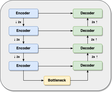
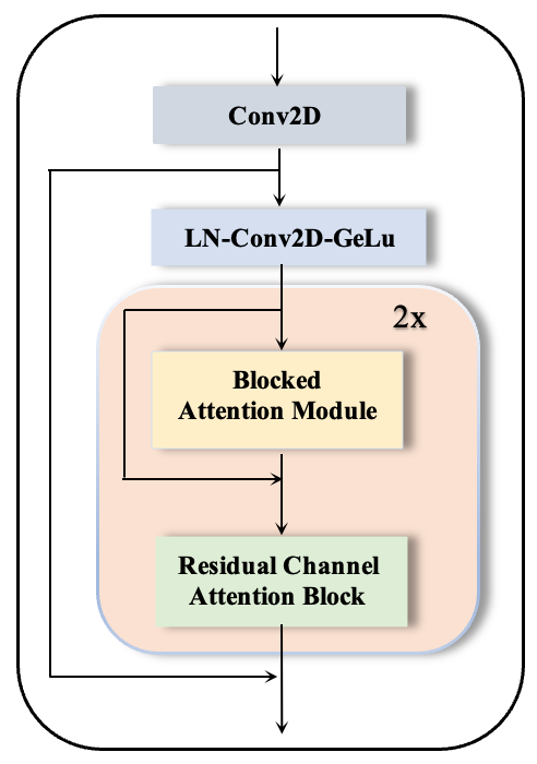
(a)	(b)

Figure 1: (a) Overall framework of the proposed method , (b) Encoder/Decoder/Bottleneck architecture. For Decoder, attention module is Base Blocked Attention Module illustrated in Figure 9. For Encoder & Bottleneck, Blocked Attention module is illustrated in Figure 3. LN represents Layer-norm.

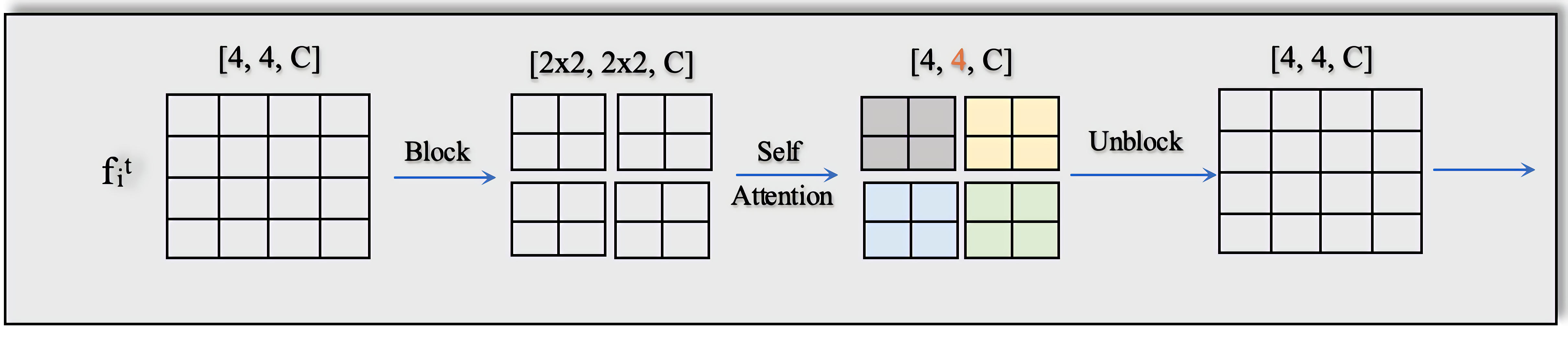
Figure 2: Base Blocked Attention Module. This figure explains the process from blocking to unblocking

3.2 Proposed Dual Self-Cross Attention Module

To introduce inter-frame interactions into our base model, we use cross-attention between feature maps of two neighboring frames. This cross-attention is computed in addition to the self-attention for each of the frames as described in Equation (1). We refer to our module as a dual self-cross attention feature extraction module. Specifically, to process a given frame $\mathbf{y}_{t}$, our model also takes past and future frames $\{\mathbf{y}_{t-1},\mathbf{y}_{t+1}\}$ in addition to the current frame $\mathbf{y}_{t}$ as input. Then, Encoder $i$ takes three sets of features $\{\mathbf{f}^{t-1}_{i},\mathbf{f}^{t}_{i},\mathbf{f}^{t+1}_{i}\}$ as input and processes them using self and cross attention followed by feature fusion to produce $\{\mathbf{f}^{t-1}_{i+1},\mathbf{f}^{t}_{i+1},\mathbf{f}^{t+1}_{i+1}\}$. We first describe the cross-attention computation for any two frames and then describe the all the computations for three neighboring frames in our dual self-cross attention module.

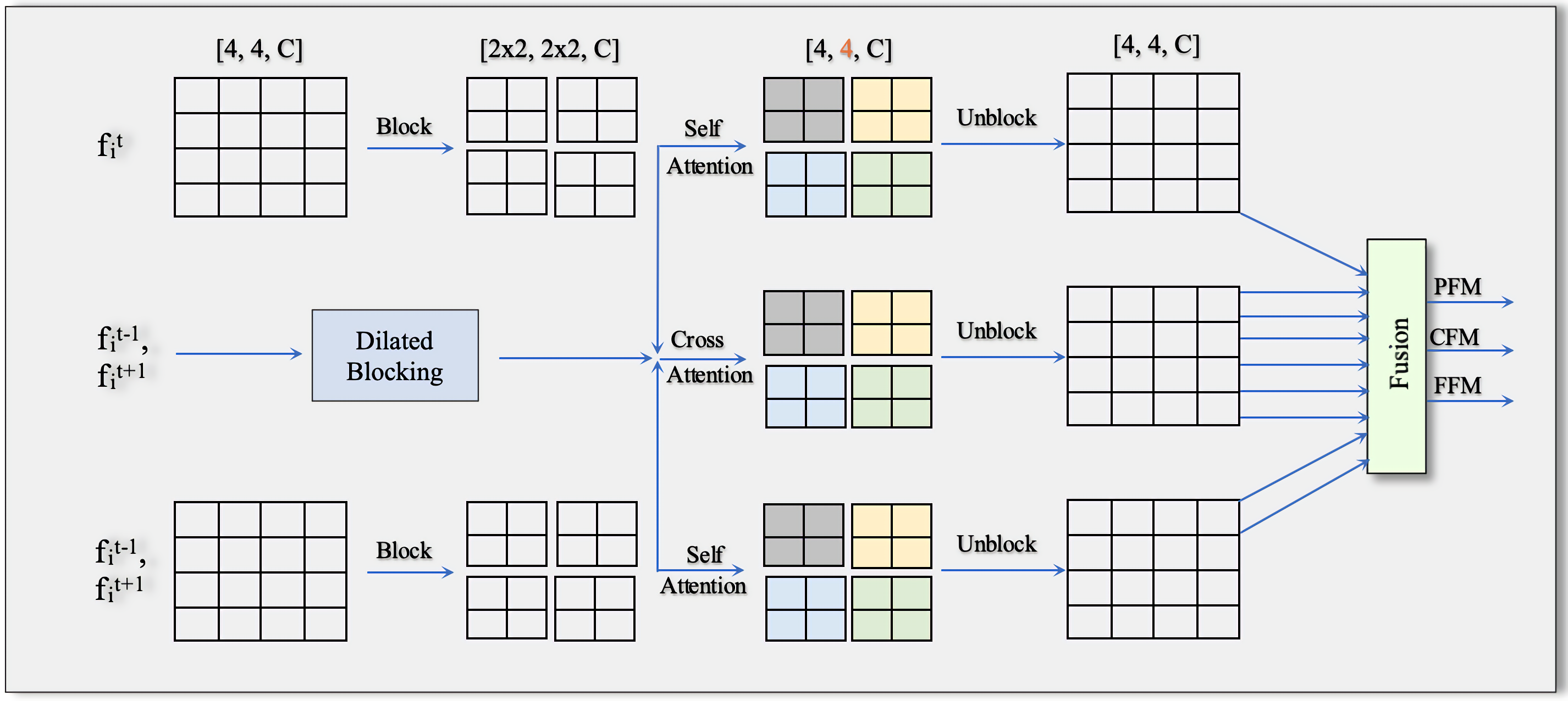
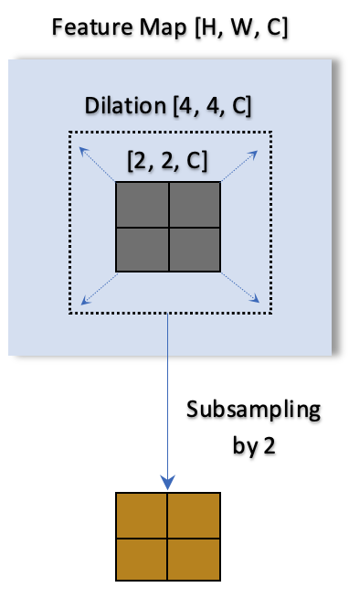
(a)	(b)

Figure 3: (a) Encoder/Bottleneck Attention Module. We perform blocking for $\{f^{t-1}_{i},f^{t}_{i},f^{t+1}_{i}\}$ and dilated blocking for $\{f^{t-1}_{i},f^{t+1}_{i}\}$, which we use to compute three self attention maps and six cross & dilated cross attention maps. (b) Dilated Blocking. To get a dilated block of size $b\times b$, we divide the given feature map into $2b\times 2b$ overlapping blocks and then subsample these blocks by a factor of 2. For better understanding on these attention maps, see Figure 4. We fuse these maps, to get past feature map (PFM), current feature map (CFM) and future feature map (FFM).

Cross Attention: Consider features $\mathbf{f}^{t-1}_{i}$ and $\mathbf{f}^{t}_{i}$. To process $\mathbf{f}^{t}_{i}$ using cross-attention with $\mathbf{f}^{t-1}_{i}$, we first block them as described in Figure 3 to obtain $\mathbf{f}_{ij}^{t-1}$ and $\mathbf{f}_{ij}^{t}$, where $j\in\{1,2,\ldots,\frac{H_{i}}{b}\times\frac{W_{i}}{b}\}$. We then linearly project $\mathbf{f}_{ij}^{t-1}$ using the matrices $P_{ih}^{K}$ and $P_{ih}^{V}$ to compute key $K_{ijh}^{t-1}$ and value $V_{ijh}^{t-1}$ respectively for head $h$. We also project features $\mathbf{f}^{t}_{ij}$ using $P_{ih}^{Q}$ to compute query $Q_{ijh}^{t}$. We now compute the cross-attention output between features in frame $t$ and $t-1$ as

$$CA_{ijh}(t,t-1)=\left[\operatorname{SoftMax}\left(Q_{ijh}^{t}\left(K_{ijh}^{t-1}\right)^{T}/\sqrt{C_{i}}\right)\right]V_{ijh}^{t-1},$$ (2)

where we compute SoftMax in row-wise fashion as before. We concatenate the features from all the heads to obtain $CA_{ij}(t,t-1)$. Note that by reversing the roles of $t$ and $t-1$, we obtain $CA_{ij}(t-1,t)$ which is a processed version of $\mathbf{f}_{i}^{t-1}$.

$CA_{ij}(t,t-1)$ computes a cross-attention between blocks centered at the same location across frames. However, in case of large motion, many of the pixels in $\mathbf{f}_{ij}^{t}$ may not present in $\mathbf{f}_{ij}^{t-1}$. To address this, we further compute cross-attention between $\mathbf{f}_{ij}^{t}$ and a dilated version of $\mathbf{f}_{ij}^{t-1}$. We denote this as $DCA_{ij}(t,t-1)$. Figure 3 explains the method to get the dilated version of a given feature map. The feature maps for all the blocks are then unblocked to obtain $CA_{i}(t,t-1)$ and $DCA_{i}(t,t-1)$.

Figure 4: Multiple Self-Cross Dilated Attention. We get past,current and future frame feature maps for next stage by fusing attentions of all blue, green and black color arrows separately.

We use the cross and dilated cross attention modules to output different attention maps for $\mathbf{f}_{i}^{t-1}$, $\mathbf{f}_{i}^{t}$ and $\mathbf{f}_{i}^{t+1}$. We illustrate all the feature maps in Figure 4. For $\mathbf{f}_{i}^{t}$, we compute five attention maps in total as $CA^{i}(t,t-1)$, $DCA^{i}(t,t-1)$, $CA_{i}(t,t+1)$, $DCA_{i}(t,t+1)$ and $SA_{i}(t)$. For $\mathbf{f}_{i}^{t-1}$, we compute $SA_{i}(t-1)$ and $CA_{i}(t-1,t)$, and for $\mathbf{f}_{i}^{t+1}$, we compute $SA_{i}(t+1)$ and $CA_{i}(t+1,t)$. We fuse these attention maps through convex combinations where the weights corresponding to a given attention map are computed by passing them through a convolutional layer and taking softmax. We explain this through a figure in the supplementary. For example, we output weight maps corresponding to each attention map $CA^{i}(t,t-1)$, $DCA^{i}(t,t-1)$, $CA_{i}(t,t+1)$, $DCA_{i}(t,t+1)$ and $SA_{i}(t)$ through a convolutional layer and apply softmax on the output to obtain weights and combine the attention maps. Thus, the fusion process is adaptive as the weights depend on the corresponding attention. The output of fusion module is further processed with RCAB [Woo et al.(2018)Woo, Park, Lee, and Kweon] to produce $f^{t}_{i+1}$.

After completion of all multi-stages of encoder and the bottleneck, for $N$ stages, we get $\{f^{t-1}_{N+1},f^{t}_{N+1},f^{t+1}_{N+1}\}$. Since all the information across frames has been mixed in various encoders, we only use the current frame feature map $f^{t}_{N+1}$ and process it further in the decoder. Thus the decoder architecture remains the same as discussed in the Base Model. After the final stage of the decoder, we apply a single convolutional layer to get a temporally stable enhanced frame.

4 Experiments & Results

4.1 Experimental Setup

We perform experiments by training on static video datasets and testing on datasets with dynamic videos. In particular we adopt three experimental settings.

Setting 1: We train on static RGB videos obtained from the DRV Dataset [Chen et al.(2019)Chen, Chen, Do, and Koltun] and evaluate on the dynamic videos. In particular, since the low light videos are available in RAW format, we convert them to RGB using the python library libraw and reduce the spatial resolution to 832 $\times$ 1248. There are 202 low light static video sequences each with 110 frames for which the long exposure ground truth is available. We train on 153 videos similar to [Chen et al.(2019)Chen, Chen, Do, and Koltun]. We test on 22 dynamic low light videos for which no ground truth is available. This is the most realistic setting that one encounters in the real-world.

Setting 2: We generate 153 static low light videos using frames from the videos in the DAVIS dataset [Khoreva et al.(2018)Khoreva, Rohrbach, and Schiele]. In particular, we apply a gamma transform on a given frame and add multiple instances of noise similar to [Zhang et al.(2021)Zhang, Li, You, and Fu] to generate a static video sequence. We then test on 30 synthetically generated low light dynamic videos from the DAVIS test dataset obtained similar to [Zhang et al.(2021)Zhang, Li, You, and Fu]. We note that while the motion in the above videos is realistic, the distortions are synthetically generated.

Setting 3: In this setting, we consider realistic distortions but synthetic motion. In particular, we introduce camera motion in the static videos in the DRV dataset described in Setting 1. We estimate the depth of the videos using Midas [Ranftl et al.(2022)Ranftl, Lasinger, Hafner, Schindler, and Koltun] and apply different camera trajectories from KITTI camera poses [Geiger et al.(2013)Geiger, Lenz, Stiller, and Urtasun] and VEED [Kanchana et al.(2022)Kanchana, Somraj, Yadwad, and Soundararajan] to generate videos with motion. Since some of the generated videos can contain disocclusions, we select a subset of 96 videos without such artifacts for testing. Each video contains 10 frames of resolution 832 $\times$ 1248. We refer to this dataset as the DRV Dataset with Synthetic Motion (DRV-SM). We use the static videos described in Setting 1 for training.

We note that ground truth videos are available for performance evaluation in Setting 2 and 3. We evaluate the methods using peak signal to noise ratio (PSNR), structural similarity index (SSIM) [Wang et al.(2004)Wang, Bovik, Sheikh, and Simoncelli] and spatio-temporal entropic differences (ST-RRED) [Soundararajan and Bovik(2012)]. For Setting 1, we evaluate through a subjective study.

4.2 Implementation Details

While training on static videos, we select three consecutive frames from each sequence. We choose a spatial patch size of 384 $\times$ 384. We train our model with a combination of VGG loss [Simonyan and Zisserman(2014)] and mean squared error loss and use Adam Optimizer [Kingma and Ba(2014)]. In all the settings, we train our model for 900 epochs; where we use a learning rate of 1e-4. The batch size is set to 2. We implement our architecture using PyTorch and use an NVIDIA DGX Version 4.6.0 GPU with 32 GB of memory to train our model.

4.3 Performance Evaluation and Comparison

We compare with state of the art low light video enhancement methods such as SMID [Chen et al.(2019)Chen, Chen, Do, and Koltun] and MBLLVEN [Lv et al.(2018)Lv, Lu, Wu, and Lim]. We compare with SMID by adopting the same training method based on consistency of enhanced output for restoring RGB video frames. We also compare with some of the recent video restoration methods such as FastDVDnet [Tassano et al.(2020)Tassano, Delon, and Veit] and VRT [Liang et al.(2022)Liang, Cao, Fan, Zhang, Ranjan, Li, Timofte, and Van Gool]. We discuss issues with comparison of low light video enhancement methods based on data generation in the supplementary. All these competing methods are trained and tested similar to our approach as described in Settings 1, 2 and 3. We first present visual examples of our results in Figure 5 corresponding to each of the experimental settings. We clearly see that our method outperforms all the other methods. In particular, generic video restoration methods fail when they are trained on static videos and tested on dynamic videos. While SMID [Chen et al.(2019)Chen, Chen, Do, and Koltun] performs better, our method outputs even better results with superior enhancement and clear visibility of details.

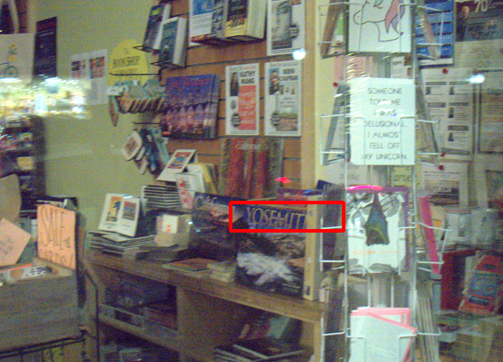
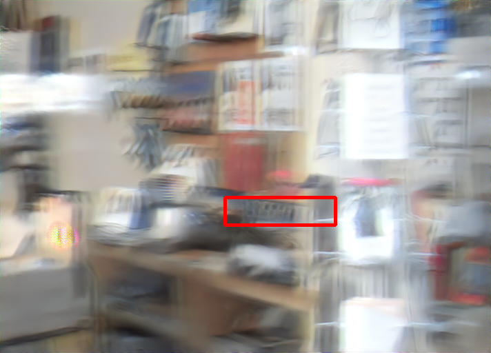
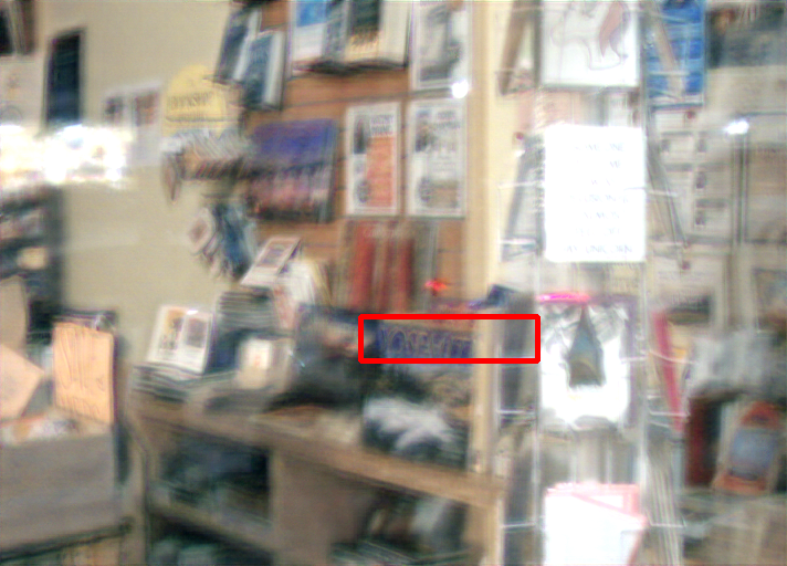
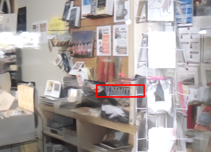
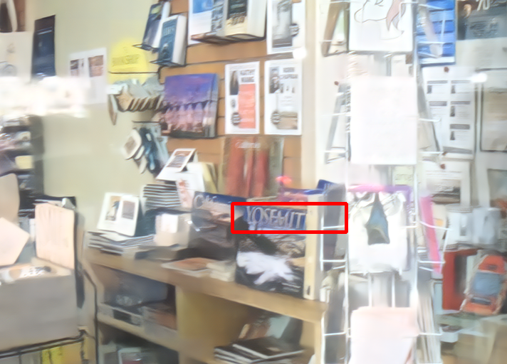
Low-Light

FastDVDNet

VRT

MBLLVEN

SMID

Ours

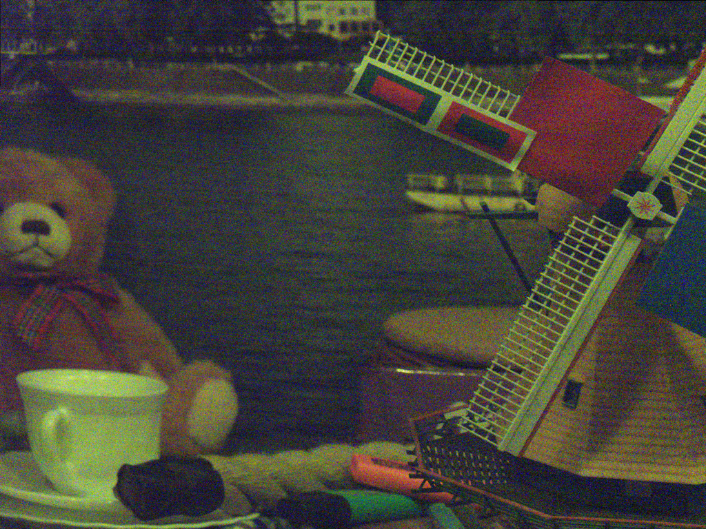
Low-Light

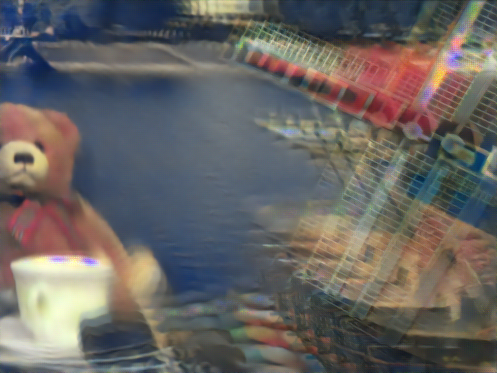
FastDVDNet

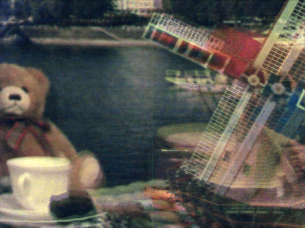
VRT

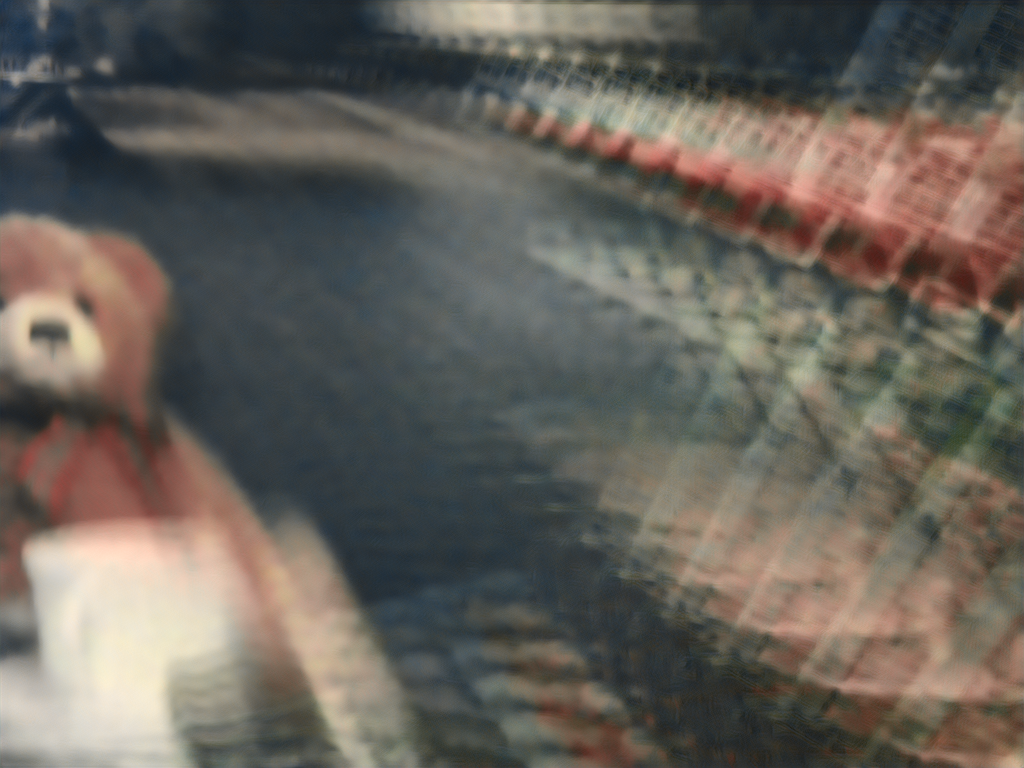
MBLLVEN

SMID

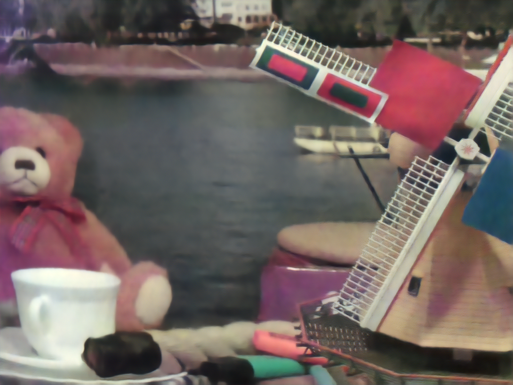
Ours

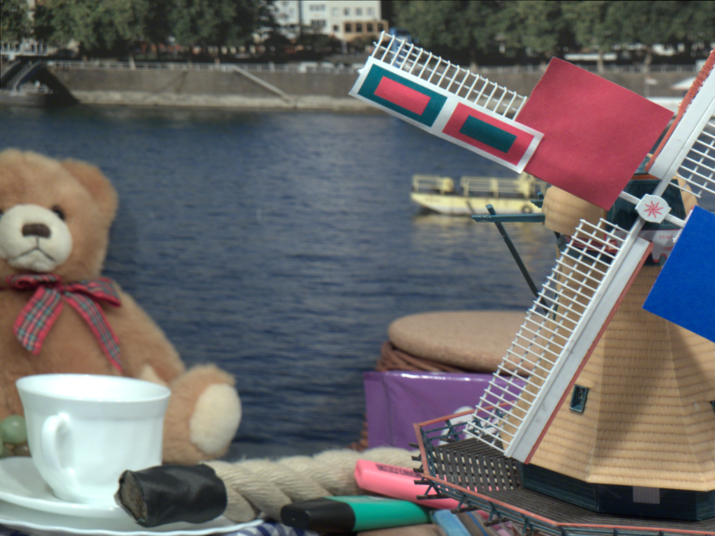
Ground Truth

Figure 5: Example frames of low-light videos enhanced using various methods. The videos in the $1^{st}$, $2^{nd}$ and $3^{rd}$ rows correspond to Setting 1, 2 and 3 as described in Section 4.1. Note that the enhanced frames from our method are sharp and have better perceptual quality when compared to SMID [Chen et al.(2019)Chen, Chen, Do, and Koltun]. Zoom-in for better viewing.

In Table 1, we present the numerical comparisons on the DAVIS (Setting 2) and DRV-SM datasets (Setting 3), since a ground truth video is available. We see that our method performs better than the other methods for both the settings corresponding to realistic motion and realistic low light distortions. We also see in Figure 6(a) that our model achieves a very good performance with very few parameters when compared to other methods.

Table 1: Quantitative Evaluation for Setting 2 and 3

Methods		Setting 2 (DAVIS)			Setting 3 (DRV-SM)
	SSIM ${\uparrow}$	ST-RRED${\downarrow}$	PSNR${\uparrow}$	SSIM${\uparrow}$	ST-RRED${\downarrow}$	PSNR${\uparrow}$
SMID [Chen et al.(2019)Chen, Chen, Do, and Koltun]	0.63	682	28.63	0.55	1248	28.64
MBLLVEN [Lv et al.(2018)Lv, Lu, Wu, and Lim]	0.43	2679	28.09	0.50	3628	28.38
FastDVDNet [Tassano et al.(2020)Tassano, Delon, and Veit]	0.60	1624	28.36	0.54	2317	28.45
VRT [Liang et al.(2022)Liang, Cao, Fan, Zhang, Ranjan, Li, Timofte, and Van Gool]	0.43	955	27.85	0.52	1882	28.47
Ours	0.82	241	29.02	0.60	745	28.92

Subjective Evaluation on Dynamic DRV Dataset: We evaluate the results on the dynamic videos of the DRV dataset through a pairwise subjective study since the ground truth videos are not available. In particular, we compare the performance of our method against SMID, which is the second best approach in Table 1. The subjective study involved 10 subjects who compared these methods on an LG (27 Inch) IPS Monitor. Our results in Figure 6(b) indicate that out of 22 dynamic video sequences, our approach was rated as better than SMID on 19 videos and on the remaining 3, the ratings were equally split between our model and SMID.

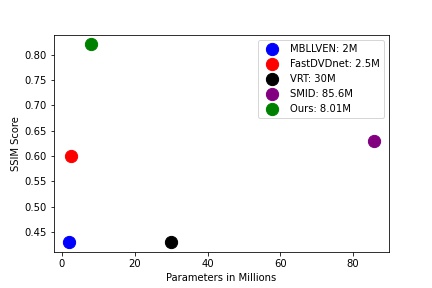
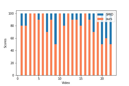
(a)	(b)

Figure 6: (a) Number of Parameters vs SSIM, (b) Subjective Study on Dynamic DRV Dataset (Setting 1)

4.4 Ablation Study

We evaluate the importance of various components of our model in Figure 7(a) corresponding to Setting 2 using ST-RRED. We see that our final model improves on both the baseline model and the model without dilation. This shows that the cross-attention module helps account for the motion although it is only trained on static sequences. Further, the dilated attention maps help account for larger motion between neighboring frames. We also see a minor improvement as we increase the dilation factor from 2 to 3. We also evaluate the performance variation with respect to the number of stages corresponding to the number of encoders in our model. We see in Figure 7(a) that the performance improves with the number of encoders and the gains tend to decrease with more scales. Although the performance could improve with more scales, we limit to 4 scales due to memory constraints.

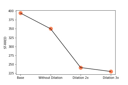
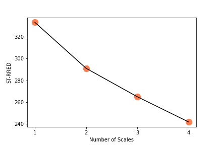
(a)	(b)

Figure 7: (a) Ablation evaluation of our models, (b) Performance variation with number of encoders

4.5 Performance on Static DRV Dataset

Although our primary objective was in the performance evaluation of the dynamic videos, here we also evaluate the performance of our method on the static videos in the DRV dataset referred to as Static DRV dataset [Chen et al.(2019)Chen, Chen, Do, and Koltun]. The models are all trained on the same static sequences mentioned in Setting 1, but now evaluated on the test set of Static DRV dataset consisting of 49 video sequences. In particular, we test on the first 10 frames from each of these static sequences in Table 2. We evaluate using SSIM and PSNR since there is no motion in the video sequences. We note that there is no clear winner with respect to different performance measures and our approach is competitive with the best. To summarize, our model matches the performance of other methods on static sequences, yet achieves a significantly better performance on dynamic videos.

Table 2: Performance On Static DRV Dataset

Methods	SSIM ${\uparrow}$	PSNR ${\uparrow}$
SMID[Chen et al.(2019)Chen, Chen, Do, and Koltun]	0.63	28.43
MBLLVEN[Lv et al.(2018)Lv, Lu, Wu, and Lim]	0.58	28.36
FastDVDNet[Tassano et al.(2020)Tassano, Delon, and Veit]	0.62	28.52
VRT[Liang et al.(2022)Liang, Cao, Fan, Zhang, Ranjan, Li, Timofte, and Van Gool]	0.53	28.37
Ours	0.61	28.53

5 Conclusion

We explored the use of attention based modules for learning of low light video enhancement on static videos for their application on dynamic videos. We showed that these attention modules can obviate the need for explicit optical flow estimation yet account for inter-frame interactions even though the interaction dynamics are different between training and testing. We achieve superior performance than other methods on multiple datasets. Our approach may also be relevant for generic video restoration.

Supplemental Materials

6 Architecture of Fusion Module

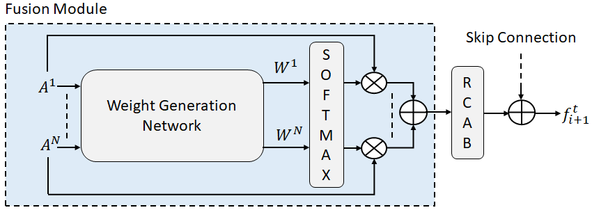
Figure 8: Block diagram illustrating our fusion module

In this section, we describe the adaptive fusion for $N$ attention maps (see Figure 8), $\{A^{1},A^{2},\ldots,A^{N}\}$. We pass each of these maps through a convolutional layer and get $W^{n}$ for $n=1,2,\ldots,N$, where each $W^{n}$ is a single channel map. The same map will be used to determine the weights for all the channels in the attention map. Finally, to obtain the mixing weights for $A^{n}$ at each location, we apply a softmax operation at each spatial location across all the $N$ maps. The resulting weights are used to fuse the attention map followed by the residual channel attention block (RCAB).

7 Ablation on DRV-SM Dataset

We evaluated the importance of various components of our model, in particular, cross-attention and dilated cross-attention with respect to our base line model on the DAVIS dataset in the main paper. Here we present similar results on the DRV-SM dataset using the ST-RRED quality measure in Figure 9. We see consistent improvements with respect to our ideas even in the DRV-SM dataset.

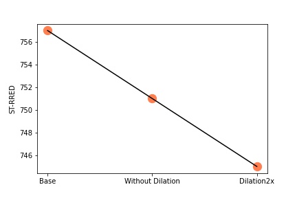
Figure 9: Ablation Evaluation on our model with DRV-SM dataset

8 Comparison with Data Generation based Methods

We now describe our experiments in comparing with a data generation method for training low light video enhancement [Triantafyllidou et al.(2020)Triantafyllidou, Moran, McDonagh, Parisot, and Slabaugh]. SIDGAN adopts a two-step procedure to generate realistic low light videos from high quality videos in the Vimeo dataset [vimeo]. In particular, a pair of cycle-GANs is used where the first cycle-GAN generates sensor specific long exposure video frames from which a second cycle-GAN generates short exposure video frames. Thus, paired labelled data is created which can be used to train deep network. However, we observe that each cycle-GAN generates very poor quality images in our experiments as shown in Figure 10. Thus we did not proceed with training the enhancement model. We believe that poor quality of video frames could perhaps be attributed to the larger image resolutions that we operate with when compared to SIDGAN [Triantafyllidou et al.(2020)Triantafyllidou, Moran, McDonagh, Parisot, and Slabaugh]. Due to memory constraints, we are not able to experiment with larger patch sizes in their model which could potentially improve performance.

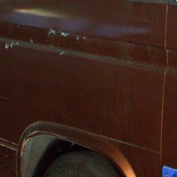
Figure 10: Examples of images generated using the SIDGAN [Triantafyllidou et al.(2020)Triantafyllidou, Moran, McDonagh, Parisot, and Slabaugh]. First column are the ground truth images from the Vimeo dataset. Second column contains outputs from first stage of SIDGAN of transforming Vimeo ground truth to sensor specific ground truths from the DRV dataset. Third column contains ground truth images from the DRV dataset and the last column contains outputs of the second stage of the SIDGAN of transforming images from third column to low light from the DRV dataset. Note that the generated images appear unnatural.

References

- [Cao et al.(2021)Cao, Li, Zhang, and Van Gool] Jiezhang Cao, Yawei Li, Kai Zhang, and Luc Van Gool. Video super-resolution transformer. arXiv preprint arXiv:2106.06847, 2021.
- [Chen et al.(2019)Chen, Chen, Do, and Koltun] Chen Chen, Qifeng Chen, Minh Do, and Vladlen Koltun. Seeing motion in the dark. In 2019 IEEE/CVF International Conference on Computer Vision (ICCV), pages 3184–3193, 2019. 10.1109/ICCV.2019.00328.
- [Eilertsen et al.(2019)Eilertsen, Mantiuk, and Unger] Gabriel Eilertsen, Rafal K Mantiuk, and Jonas Unger. Single-frame regularization for temporally stable cnns. In Proceedings of the IEEE/CVF Conference on Computer Vision and Pattern Recognition, pages 11176–11185, 2019.
- [Geiger et al.(2013)Geiger, Lenz, Stiller, and Urtasun] Andreas Geiger, Philip Lenz, Christoph Stiller, and Raquel Urtasun. Vision meets robotics: The kitti dataset. The International Journal of Robotics Research, 32(11):1231–1237, 2013.
- [Jiang and Zheng(2019)] Haiyang Jiang and Yinqiang Zheng. Learning to see moving objects in the dark. In Proceedings of the IEEE/CVF International Conference on Computer Vision, pages 7324–7333, 2019.
- [Kanchana et al.(2022)Kanchana, Somraj, Yadwad, and Soundararajan] Vijayalakshmi Kanchana, Nagabhushan Somraj, Suraj Yadwad, and Rajiv Soundararajan. Revealing disocclusions in temporal view synthesis through infilling vector prediction. In Proceedings of the IEEE/CVF Winter Conference on Applications of Computer Vision, pages 3541–3550, 2022.
- [Khoreva et al.(2018)Khoreva, Rohrbach, and Schiele] Anna Khoreva, Anna Rohrbach, and Bernt Schiele. Video object segmentation with language referring expressions. In Asian Conference on Computer Vision, pages 123–141. Springer, 2018.
- [Kingma and Ba(2014)] Diederik P Kingma and Jimmy Ba. Adam: A method for stochastic optimization. arXiv preprint arXiv:1412.6980, 2014.
- [Lai et al.(2018)Lai, Huang, Wang, Shechtman, Yumer, and Yang] Wei-Sheng Lai, Jia-Bin Huang, Oliver Wang, Eli Shechtman, Ersin Yumer, and Ming-Hsuan Yang. Learning blind video temporal consistency. In Proceedings of the European conference on computer vision (ECCV), pages 170–185, 2018.
- [Li et al.(2020)Li, Li, Fang, Li, and Zhang] Jiaqian Li, Juncheng Li, Faming Fang, Fang Li, and Guixu Zhang. Luminance-aware pyramid network for low-light image enhancement. IEEE Transactions on Multimedia, pages 1–1, 2020. 10.1109/TMM.2020.3021243.
- [Liang et al.(2022)Liang, Cao, Fan, Zhang, Ranjan, Li, Timofte, and Van Gool] Jingyun Liang, Jiezhang Cao, Yuchen Fan, Kai Zhang, Rakesh Ranjan, Yawei Li, Radu Timofte, and Luc Van Gool. Vrt: A video restoration transformer. arXiv preprint arXiv:2201.12288, 2022.
- [Lim and Kim(2020)] Seokjae Lim and Wonjun Kim. Dslr: Deep stacked laplacian restorer for low-light image enhancement. IEEE Transactions on Multimedia, pages 1–1, 2020. 10.1109/TMM.2020.3039361.
- [Liu et al.(2021)Liu, Ma, Zhang, Fan, and Luo] Risheng Liu, Long Ma, Jiaao Zhang, Xin Fan, and Zhongxuan Luo. Retinex-inspired unrolling with cooperative prior architecture search for low-light image enhancement. In Proceedings of the IEEE/CVF Conference on Computer Vision and Pattern Recognition, pages 10561–10570, 2021.
- [Lv et al.(2018)Lv, Lu, Wu, and Lim] Feifan Lv, Feng Lu, Jianhua Wu, and Chongsoon Lim. Mbllen: Low-light image/video enhancement using cnns. In BMVC, volume 220, page 4, 2018.
- [Ranftl et al.(2022)Ranftl, Lasinger, Hafner, Schindler, and Koltun] René Ranftl, Katrin Lasinger, David Hafner, Konrad Schindler, and Vladlen Koltun. Towards robust monocular depth estimation: Mixing datasets for zero-shot cross-dataset transfer. IEEE Transactions on Pattern Analysis and Machine Intelligence, 44(3):1623–1637, 2022. 10.1109/TPAMI.2020.3019967.
- [Ronneberger et al.(2015)Ronneberger, Fischer, and Brox] Olaf Ronneberger, Philipp Fischer, and Thomas Brox. U-net: Convolutional networks for biomedical image segmentation. In International Conference on Medical image computing and computer-assisted intervention, pages 234–241. Springer, 2015.
- [Simonyan and Zisserman(2014)] Karen Simonyan and Andrew Zisserman. Very deep convolutional networks for large-scale image recognition. arXiv preprint arXiv:1409.1556, 2014.
- [Soundararajan and Bovik(2012)] Rajiv Soundararajan and Alan C Bovik. Video quality assessment by reduced reference spatio-temporal entropic differencing. IEEE Transactions on Circuits and Systems for Video Technology, 23(4):684–694, 2012.
- [Tassano et al.(2020)Tassano, Delon, and Veit] Matias Tassano, Julie Delon, and Thomas Veit. Fastdvdnet: Towards real-time deep video denoising without flow estimation. In Proceedings of the IEEE/CVF Conference on Computer Vision and Pattern Recognition, pages 1354–1363, 2020.
- [Triantafyllidou et al.(2020)Triantafyllidou, Moran, McDonagh, Parisot, and Slabaugh] Danai Triantafyllidou, Sean Moran, Steven McDonagh, Sarah Parisot, and Gregory Slabaugh. Low light video enhancement using synthetic data produced with an intermediate domain mapping, 2020. URL https://arxiv.org/abs/2007.09187.
- [Vaswani et al.(2017a)Vaswani, Shazeer, Parmar, Uszkoreit, Jones, Gomez, Kaiser, and Polosukhin] Ashish Vaswani, Noam Shazeer, Niki Parmar, Jakob Uszkoreit, Llion Jones, Aidan N Gomez, Łukasz Kaiser, and Illia Polosukhin. Attention is all you need. Advances in neural information processing systems, 30, 2017a.
- [Vaswani et al.(2017b)Vaswani, Shazeer, Parmar, Uszkoreit, Jones, Gomez, Kaiser, and Polosukhin] Ashish Vaswani, Noam Shazeer, Niki Parmar, Jakob Uszkoreit, Llion Jones, Aidan N Gomez, Łukasz Kaiser, and Illia Polosukhin. Attention is all you need. Advances in neural information processing systems, 30, 2017b.
- [Wang et al.(2020)Wang, Liu, Siu, and Lun] Li-Wen Wang, Zhi-Song Liu, Wan-Chi Siu, and Daniel PK Lun. Lightening network for low-light image enhancement. IEEE Transactions on Image Processing, 29:7984–7996, 2020.
- [Wang et al.(2019)Wang, Chan, Yu, Dong, and Change Loy] Xintao Wang, Kelvin CK Chan, Ke Yu, Chao Dong, and Chen Change Loy. Edvr: Video restoration with enhanced deformable convolutional networks. In Proceedings of the IEEE/CVF Conference on Computer Vision and Pattern Recognition Workshops, pages 0–0, 2019.
- [Wang et al.(2004)Wang, Bovik, Sheikh, and Simoncelli] Zhou Wang, Alan C Bovik, Hamid R Sheikh, and Eero P Simoncelli. Image quality assessment: from error visibility to structural similarity. IEEE transactions on image processing, 13(4):600–612, 2004.
- [Woo et al.(2018)Woo, Park, Lee, and Kweon] Sanghyun Woo, Jongchan Park, Joon-Young Lee, and In So Kweon. Cbam: Convolutional block attention module. In Proceedings of the European conference on computer vision (ECCV), pages 3–19, 2018.
- [Wu et al.(2022)Wu, Weng, Zhang, Wang, Yang, and Jiang] Wenhui Wu, Jian Weng, Pingping Zhang, Xu Wang, Wenhan Yang, and Jianmin Jiang. Uretinex-net: Retinex-based deep unfolding network for low-light image enhancement. In Proceedings of the IEEE/CVF Conference on Computer Vision and Pattern Recognition, pages 5901–5910, 2022.
- [Yang et al.(2020)Yang, Wang, Fang, Wang, and Liu] Wenhan Yang, Shiqi Wang, Yuming Fang, Yue Wang, and Jiaying Liu. From fidelity to perceptual quality: A semi-supervised approach for low-light image enhancement. In Proceedings of the IEEE/CVF Conference on Computer Vision and Pattern Recognition, pages 3063–3072, 2020.
- [Zhang et al.(2021)Zhang, Li, You, and Fu] Fan Zhang, Yu Li, Shaodi You, and Ying Fu. Learning temporal consistency for low light video enhancement from single images. In Proceedings of the IEEE/CVF Conference on Computer Vision and Pattern Recognition, pages 4967–4976, 2021.
- [Zhang et al.(2022)Zhang, Zheng, Hong, Xu, Yan, and Wang] Zhao Zhang, Huan Zheng, Richang Hong, Mingliang Xu, Shuicheng Yan, and Meng Wang. Deep color consistent network for low-light image enhancement. In Proceedings of the IEEE/CVF Conference on Computer Vision and Pattern Recognition, pages 1899–1908, 2022.
- [Zhao et al.(2021a)Zhao, Zhang, Chen, Metaxas, and Zhang] Long Zhao, Zizhao Zhang, Ting Chen, Dimitris Metaxas, and Han Zhang. Improved transformer for high-resolution gans. Advances in Neural Information Processing Systems, 34, 2021a.
- [Zhao et al.(2021b)Zhao, Xiong, Wang, Ou, Yu, and Kuang] Zunjin Zhao, Bangshu Xiong, Lei Wang, Qiaofeng Ou, Lei Yu, and Fa Kuang. Retinexdip: A unified deep framework for low-light image enhancement. IEEE Transactions on Circuits and Systems for Video Technology, pages 1–1, 2021b. 10.1109/TCSVT.2021.3073371.