Observation of edge magnetoplasmon squeezing in a quantum Hall conductor

Abstract

Squeezing of the quadratures of the electromagnetic field has been extensively studied in optics and microwaves. However, previous works focused on the generation of squeezed states in a low impedance ($Z_{0}\approx 50\Omega$) environment. We report here on the demonstration of the squeezing of bosonic edge magnetoplasmon modes in a quantum Hall conductor whose characteristic impedance is set by the quantum of resistance ($R_{K}\approx 25k\Omega$), offering the possibility of an enhanced coupling to low-dimensional quantum conductors. By applying a combination of dc and ac drives to a quantum point contact, we demonstrate squeezing and observe a noise reduction 18% below the vacuum fluctuations. This level of squeezing can be improved by using more complex conductors, such as ac driven quantum dots or mesoscopic capacitors.

In quantum Hall conductors, charge excitations propagate ballistically along one dimensional chiral channels. This ballistic propagation has been exploited in electron quantum optics experiments Bocquillon2014 ; Marguerite2017 focusing on the generation and manipulation of elementary electron and hole excitations of the Fermi sea. These are particle-like fermionic excitations, but the dynamics of charge propagation along one-dimensional edge channels can be equivalently described in terms of collective bosonic excitations called edge magnetoplasmons (EMP), which consist of coherent superpositions of electron-hole pairs on top of the Fermi sea.

EMP have been largely investigated in the past by studying the propagation of the time dependent electrical current in the time Ashoori1992 ; Zhitenev1993 ; Ernst1996 ; Sukhodub2004 ; Kamata2010 ; Kumada2011 or frequency domainTalyanskii1992 ; Gabelli2007a ; Hashisaka2012 ; Delgard2021 . Experiments have highlighted the dependence of EMP propagation speed on the magnetic field and on the screening by nearby electrostatic gates. All these studies are based on a classical description of charge propagation along the edge channels which can be modeled as transmission linesHashisaka2012 . However, chiral edge channels have three important differences with respect to standard 50 Ohms coaxial cables. Firstly, the chirality results in the separation between forward and backward propagating waves. Secondly, the speed of the EMPKumada2011 is of the order of $10^{5}$m.s^-1, three orders of magnitude smaller than the speed of light, resulting in wavelengths in the $\mu$m range at GHz frequencies compared to the cm range in standard coaxial cables. EMPs would thus allow for more compact circuits. Finally, their characteristic impedance is of the order of the resistance quantum, $R_{K}\approx 25$ k$\Omega$, much larger than the 50 Ohms standard, offering the possibility of a strong coupling to low dimensional quantum conductors of high impedanceParmentier2011b .

These specificities motivated recent theoretical and experimental Viola2014 Bosco2019 studies of EMP transmission lines for efficient coupling to on-chip high impedance quantum devices, such as charge or spin qubits, for the study of Coulomb interaction effects in one-dimensional edge channels Gourmelon2020 , or for the realization of on-chip microwave circulators Mahoney2017 . So far, these studies have focused on the classical regime, where EMP states can be described as coherent states. However, as for other bosonic modes, quantum EMP states can also be generated. In the last years there has been a strong interest for the generation of quantum radiation by quantum conductors Beenakker2004 ; Lebedev2010 ; Grimsmo2016 and in particular of squeezed states Mendes2015 ; Ferraro2018 ; Rebora2021 . So far, it has been limited to the study of low impedance (50 Ohms) transmission lines coupled to superconducting circuitsArmour2013 ; Mendes2019 ; Rolland2019 or tunnel junctionsGasse2013 . We report here on the generation of squeezed EMP states at the output of a quantum point contact used as an electronic beam-splitter in a GaAs quantum Hall conductor, as discussed in Ref. [Rebora2021, ]. Using two-particle interference processesMarguerite2017 occurring between electron and hole excitations colliding on the splitter, we generate a squeezed EMP vacuum state at frequency $f=\frac{\Omega}{2\pi}=7.75$ GHz at the splitter output with a noise minimum 18% below the vacuum fluctuations. The non-linear EMP scattering at the splitter breaks a $2f$ pump signal into coherent photon pairs, thereby achieving squeezing Yuen76 .

Squeezed EMP states could be used for quantum enhanced measurements in EMP interferometersHiyama2015 , or to extend the study of low dimensional quantum conductors in the regime where they are driven by quantum voltage sourcesSouquet2014 , exploiting the strong coupling of high impedance transmission lines to high impedance low-dimensional quantum circuits.

In the bosonic description of charge propagation, the charge density $\rho(x,t)$ carried by a single edge channel can be expressed as a function of a chiral bosonic field $\Phi(x,t)$ with $\rho(x,t)=\frac{-e}{\sqrt{\pi}}\partial_{x}\Phi(x,t)$. The relation between the electrical current and the field can then be deduced directly from charge conservation: $i(x,t)=\frac{e}{\sqrt{\pi}}\partial_{t}\Phi(x,t)$. At low frequency (typically a few GHz), dispersion effects can be neglected, such that $\Phi(x,t)$ can be decomposed in terms of elementary plasmon excitations at pulsation $\omega$ propagating with constant speed velocity $v$:

$$\Phi(x,t) = \frac{-i}{\sqrt{4\pi}}\sum_{\omega}\sqrt{\frac{2\pi}{\omega T_{\text{meas}}}}[b_{\omega}e^{i\omega(x/v-t)}-h.c.]$$ (1)

with $$[b_{\omega},b^{{\dagger}}_{\omega^{\prime}}]=\delta_{\omega,\omega^{\prime}}.$$ (2)

$b^{{\dagger}}_{\omega}$ is the operator which creates a single plasmon of energy $\hbar\omega$ and obeys the usual bosonic commutation relations. The long measurement time $T_{\text{meas}}$ sets the discretization of the plasmon modes by steps of $2\pi/T_{\text{meas}}$. In order to address the squeezing of EMP modes, it is useful to introduce the quadratures of the bosonic field at a given pulsation $\Omega$ defined for a phase $0\leq\varphi\leq\pi$:

$$X_{\Omega,\varphi} = \frac{b_{\Omega}e^{i\varphi}+b^{{\dagger}}_{\Omega}e^{-i\varphi}}{\sqrt{2}}$$ (3)

Their fluctuations $\langle\Delta X_{\Omega,\varphi}^{2}\rangle$ can be decomposed into an isotropic $\langle\Delta X_{\Omega,\text{iso}}^{2}\rangle$ and an anisotropic, $\varphi$ dependent, part $\langle\Delta X_{\Omega,\text{an}}^{2}\rangle$ given by:

$$\langle\Delta X_{\Omega,\text{iso}}^{2}\rangle = \langle b^{{\dagger}}_{\Omega}b_{\Omega}\rangle-\langle b^{{\dagger}}_{\Omega}\rangle\langle b_{\Omega}\rangle+\frac{1}{2}$$ (4)

$$\langle\Delta X_{\Omega,\text{an}}^{2}\rangle = \Re\left((\langle b^{2}_{\Omega}\rangle-\langle b_{\Omega}\rangle^{2})e^{2i\varphi}\right)$$ (5)

For classical coherent states, $\langle\Delta X_{\Omega,\varphi}^{2}\rangle$ is isotropic ($\langle\Delta X_{\Omega,\text{an}}^{2}\rangle=0$) and given by $\langle\Delta X_{\Omega,\varphi}^{2}\rangle=1/2$ which are called vacuum fluctuations. For squeezed states, the minimum value of the noise, obtained for a certain value $\varphi=\varphi_{0}$ of the angle, goes below the vacuum fluctuations, $\langle\Delta X_{\Omega,\varphi_{0}}^{2}\rangle<1/2$. As imposed by Heisenberg’s uncertainty principle, the orthogonal quadrature then exhibits larger fluctuations: $\langle\Delta X_{\Omega,\varphi_{0}+\pi/2}^{2}\rangle>1/2$.

The quadratures of the field and their fluctuations can be experimentally accessed from the measurements of the electrical current $i(t)$ and its fluctuations at high frequency. More precisely, defining $i_{\Omega,\varphi}(t)=\cos({\Omega t+\varphi})\;i(t)$, one has:

$$\langle\overline{i_{\Omega,\varphi}(t)}^{T_{\text{meas}}}\rangle = -2e\sqrt{\frac{\Omega}{\pi T_{\text{meas}}}}\langle X_{\Omega,\varphi}\rangle$$ (6)

$$S_{\Omega,\varphi} = 2\int d\tau\overline{\langle\delta i_{\Omega,\varphi}(t+\tau/2)\delta i_{\Omega,\varphi}(t-\tau/2)\rangle}^{T_{\text{meas}}}$$ (7)

$$= \frac{e^{2}\Omega}{2\pi}\langle\Delta X_{\Omega,\varphi}^{2}\rangle$$ (8)

where $\overline{i_{\Omega,\varphi}(t)}^{T_{\text{meas}}}$ denotes the average of $i_{\Omega,\varphi}(t)$ over the measurement time $T_{\text{meas}}$. Classical states are thus defined by current fluctuations $S_{\Omega,\varphi}=\frac{e^{2}\Omega}{4\pi}=\frac{e^{2}f}{2}$ and squeezed states by $S_{\Omega,\varphi_{0}}<\frac{e^{2}f}{2}$. Experimentally, one measures the noise in excess of the equilibrium fluctuations $\Delta S_{\Omega,\varphi}=S_{\Omega,\varphi}-\frac{e^{2}f}{2}$ and squeezing occurs when $\Delta S_{\Omega,\varphi_{0}}<0$ Note1 .

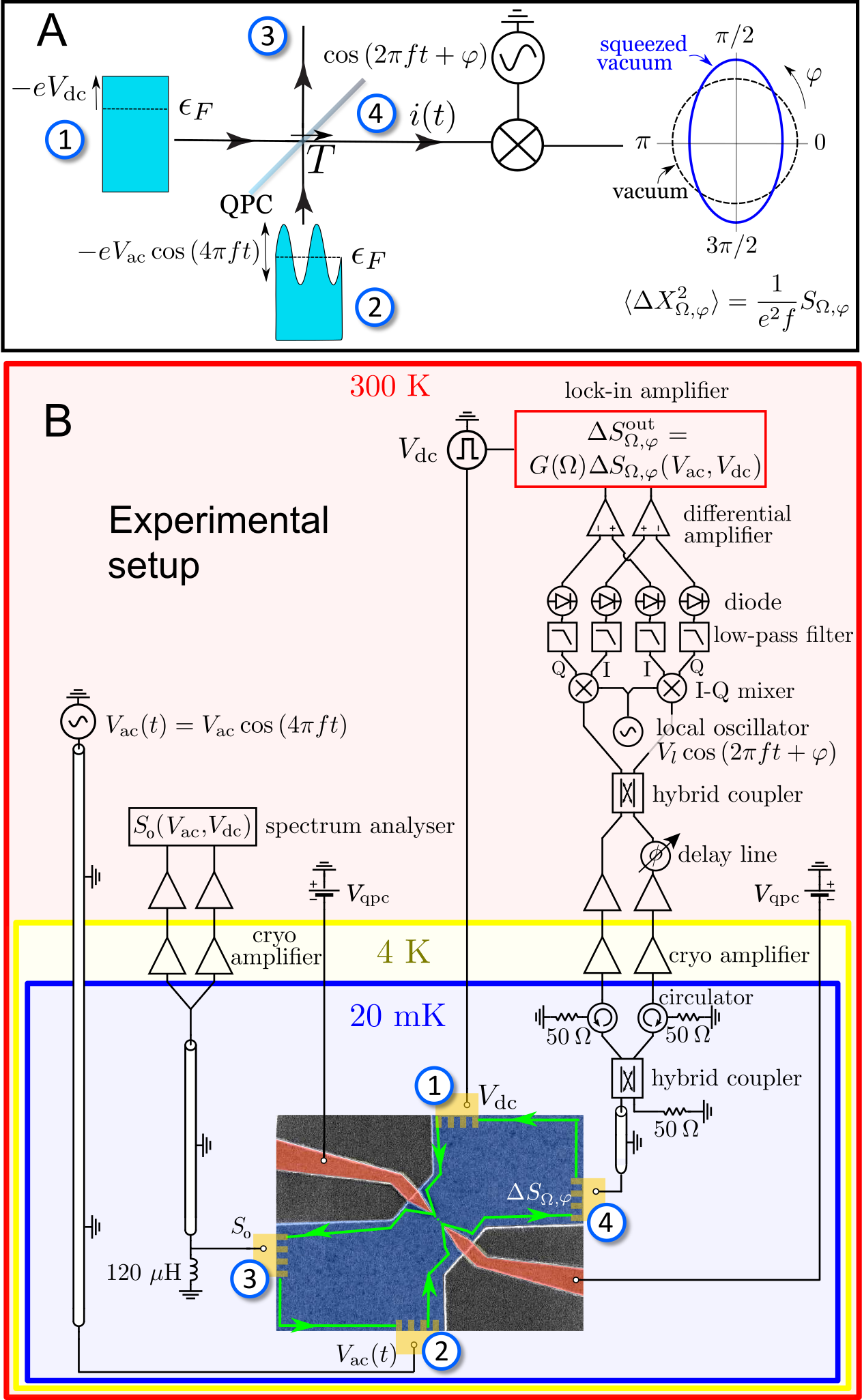
Figure 1: A. Principle of the experiment: a QPC is used as an electronic beam-splitter of transmission $T$ for the collision of electron and hole excitations generated at inputs 1 and 2. Input 1 is connected to a dc source, which shifts the chemical potential of the edge channel by $-eV_{\text{dc}}$. Input 2 is connected to an ac sinusoidal source of amplitude $V_{\text{ac}}$ and frequency $2f$. EMP squeezing is characterized at output 4 by measuring the correlations $S_{\Omega,\varphi}$ of the current $i_{\Omega,\varphi}$. For a squeezed vacuum, $S_{\Omega,\varphi}$ goes below the vacuum fluctuations for $\varphi=0$ and above them for $\varphi=\pi/2$. B. Experimental setup: the low frequency noise $\Delta S_{0}$ is measured at output 3 and the high frequency noise $\Delta S_{\Omega,\varphi}$ at output 4. The EMP current $i(t)$ is weakly transmitted to a $Z_{0}=50$ $\Omega$ coaxial cable, amplified using two cryogenic amplifiers in a double balanced configurationParmentier2011 ; Bisognin2019b and multiplied to the local oscillator $V_{l}(t)=V_{l}\cos{(2\pi ft+\varphi)}$ using high frequency mixers. The noise power is then integrated using a diode in a $800$ MHz bandwidth set by a low pass filter. The noise is measured via a lock-in detection by applying a square modulation at a frequency $f_{m}=234$ Hz to the dc voltage $V_{\text{dc}}$. The resulting output excess noise, $\Delta S_{\Omega,\varphi}^{\text{out}}$ is proportional to $\Delta S_{\Omega,\varphi}$ with a proportionality factor $G(\Omega)$ that needs to be calibrated.

The principle of the experiment is represented in Figure 1.A. A quantum point contact (QPC) is used as a beam-splitter for electronic excitations of transmission probability $T$ (and reflection probability $R=1-T$). By plugging two electronic sources at inputs 1 and 2 of the QPC, collisions between electron and hole excitationsLiu1998 ; Bocquillon2013 emitted by each source occur at the beam-splitter. Previous implementations of high frequency noise measurements Zakka-Bajjani2007 ; Bisognin2019b have focused on the single source configuration, where the quantum point contact is biased by a dc voltage $V_{\text{dc}}$. These measurements have shown that there is a voltage threshold for the generation of high frequency noise $V_{\text{dc}}=hf/q$ which can be used to measure the charge $q$ of the quasiparticles scattered by the splitterBisognin2019b . However, in this configuration, the noise is isotropic and no squeezing is obtained. By adding an ac sinusoidal source at frequency $2f$ at input 2, EMP squeezing at frequency $f$ can be obtained when both the dc voltage $V_{\text{dc}}$ and the ac voltage amplitude $V_{\text{ac}}$ are set close to the threshold $hf/q$. Squeezing is characterized by multiplying the electrical current $i(t)$ at the output of the splitter with the local oscillator $\cos({\Omega t+\varphi})$. As represented in Figure 1.A., the resulting low-frequency current correlations $S_{\Omega,\varphi}$ are expected to go beyond (respectively above) the vacuum fluctuations when the phase of the local oscillator is set to $\varphi=0$ (respectively $\varphi=\pi/2$). This approach has strong similarities with the one developed by Gasse et al. in Ref. [Gasse2013, ] where squeezing is generated in a $50$ Ohms coaxial line using a low impedance tunnel junction of resistance $R=70$ $\Omega$. As mentioned above, our work is different as it demonstrates squeezing in a high impedance $Z\approx R_{K}$ EMP transmission line allowing for a strong in situ coupling to mesoscopic circuits.

The experimental setup is represented in Figure 1.B. The conductor is a two-dimensional electron gas in a GaAs/AlGaAs heterostructure, with charge density $1.9\text{\times}{10}^{15}\text{\,}{\mathrm{m}}^{-2}$ and mobility $\mu=$2.4\text{\times}{10}^{6}\text{\,}{\mathrm{cm}}^{-2}\text{\,}{\mathrm{V}}^{-1}\text{\,}{\mathrm{s}}^{-1}$$ at 4 K. A magnetic field $B=2.6$ T is applied perpendicularly to the sample in order to reach the quantum Hall effect at filling factor $\nu=3$ where three edge channels propagate along the edges of the sample. A quantum point contact is used to partition selectively the outer edge channel on which we focus in this study. The transmission is set to $T\approx 0.5$ to generate the maximum partition noise. A dc current is generated at input 1 of the quantum point contact and the ac voltage $V_{\text{ac}}(t)=V_{\text{ac}}\cos{(4\pi ft)}$ is applied at input 2 with $f=7.75$ GHz. The measurement frequency $f=7.75$ GHz is chosen such that $k_{B}T_{\text{el}}\ll hf$, where $T_{\text{el}}$ is the electronic temperature. The high frequency noise $\Delta S_{\Omega,\varphi}(V_{\text{dc}},V_{\text{ac}})$ is measured by weakly transmitting the EMPs propagating at output 4 to a 50 Ohm coaxial line, where the weak coupling is ensured by the strong impedance mismatch between the $50$ Ohms of the coaxial cable and the impedance $R_{K}/\nu$ of the quantum Hall conductor. The signal is then amplified by a set of two double balanced cryogenic amplifiersParmentier2011 ; Bisognin2019b . $S_{\Omega,\varphi}$ is measured by multiplying the output signal with a local oscillator $V_{l}(t)=V_{l}\cos{(\Omega t+\varphi)}$ using high frequency mixers. The local oscillator is locked in phase with the pump $V_{\text{ac}}(t)$ and the phase $\varphi$ of the measured quadrature can be continuously varied. $S_{\Omega,\varphi}$ is finally measured using a diode which integrates the power at the output of the mixer in a $800$ MHz bandwidth set by a low pass filter. The typical resolution required on $S_{\Omega,\varphi}$ is smaller than $10^{-29}$ A² Hz^-1, which corresponds to the thermal noise generated by a variation of a few tens of microKelvins of a $50$ Ohm resistor. This needs to be compared to the base temperature of the fridge ($\approx 30$ mK) and to the noise temperature of the cryogenic amplifiers ($\approx 4$ K). In order to mitigate longtime variations of these two noise temperatures which could easily overcome the signal, we use a lock-in detection of the noise by modulating in time the applied dc voltage on input 1 (between $V_{\text{dc}}$ and 0) at a frequency $f_{m}=234$ Hz. The output excess high frequency noise $\Delta S^{\text{out}}_{\Omega,\varphi}(V_{\text{dc}},V_{\text{ac}})$ is proportional to $\Delta S_{\Omega,\varphi}(V_{\text{dc}},V_{\text{ac}})$ with a proportionality factor $G(\Omega)$ that takes into account both the weak coupling to the transmission line and the amplification chain.

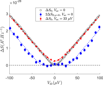
Figure 2: Measurements of $\Delta S_{0}(V_{\text{dc}},V_{\text{ac}}=0)$ (black circles) and $\Delta S_{\Omega_{\varphi}}(V_{\text{dc}},V_{\text{ac}}=0)$ (blue points) when the pump is switched off, and measurements of $\Delta S_{0}(V_{\text{dc}},V_{\text{ac}})$ when the pump is switched on with $V_{\text{ac}}=33$ $\mu$V (red points). The black and red dashed lines represent the theoretical predictions for $\Delta S_{0}$ with $V_{\text{ac}}=0$ (black dashed line) and $V_{\text{ac}}=33$ $\mu$V (red dashed line) with $T_{\text{el}}=40$ mK. The blue dashed line is the theoretical prediction for $\Delta S_{\Omega,\varphi}$ with $V_{\text{ac}}=0$ and $T_{\text{el}}=30$ mK.

We calibrate $G(\Omega)$ by measuring simultaneously the easily calibrated Note2 excess zero frequency noise $\Delta S_{0}(V_{\text{dc}},V_{\text{ac}}=0)$ (at output 3 of the splitter) and the high frequency noise $\Delta S_{\Omega,\varphi}(V_{\text{dc}},V_{\text{ac}}=0)$ (at output 4) when the pump is off, $V_{\text{ac}}=0$. In the absence of the pump, $\Delta S_{\Omega,\varphi}(V_{\text{dc}},0)$ is independent of the phase $\varphi$ and is directly related to the excess zero frequency noise shifted by the voltageRoussel2016 ; Safi2020 $\pm hf/e$:

$$\Delta S_{\Omega,\varphi}(V_{\text{dc}},0) = \frac{\Delta S_{0}(V_{\text{dc}}+hf/e)+\Delta S_{0}(V_{\text{dc}}-hf/e)}{4},$$ (9)

with $\Delta S_{0}(V_{\text{dc}}\pm hf/e)=S_{0}(V_{\text{dc}}\pm hf/e)-S_{0}(\pm hf/e)$. As can be seen from Eq. (9), for high voltages $V_{dc}>hf/e$, $\Delta S_{\Omega,\varphi}(V_{\text{dc}},0)$ varies linearly with the applied voltage with a slope $\frac{e^{3}}{h}RT$ which can be used for the determination of $G(\Omega)$. The excess low frequency noise $\Delta S_{0}(V_{\text{dc}},0)$ and the high frequency noise $2\Delta S_{\Omega,\varphi=0}(V_{\text{dc}},0)$ for $f=\frac{\Omega}{2\pi}=7.75$ GHz are plotted in Figure 2, where the constant $G(\Omega)$ has been adjusted so that $\Delta S_{\Omega,\varphi}(V_{\text{dc}},0)$ verifies Eq. (9). The black dotted line represents the standard low-frequency shot noise formula $\Delta S_{0}(V_{\text{dc}},0)=2\frac{e^{3}}{h}RTV_{\text{dc}}[\coth{\frac{eV_{\text{dc}}}{2k_{B}T_{\text{el}}}}-\frac{2k_{B}T_{\text{el}}}{eV_{\text{dc}}}]$ with $T_{\text{el}}=40$ mK and the transmission of the beam-splitter is set to $T=0.42$. The blue dashed line represents the prediction from Eq.(9) which agrees well with the data. As expected, the low frequency noise varies linearly for $eV_{\text{dc}}>k_{B}T_{el}$ which contrasts with the high frequency noise which is suppressed when $V_{\text{dc}}$ is smaller than the voltage threshold $hf/e=32$ $\mu$V for $f=7.75$ GHz.

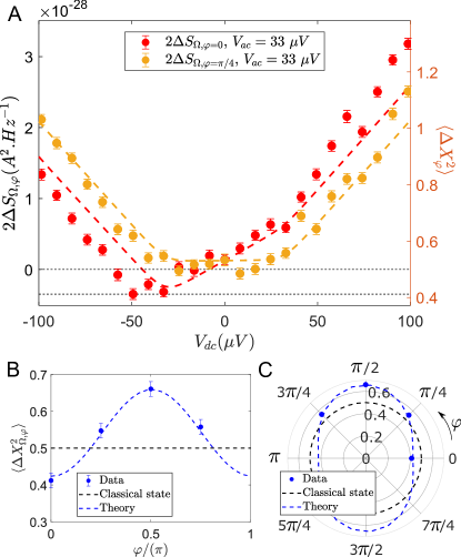
Figure 3: A. Measurements of $\Delta S_{\Omega,\varphi}$ for $\varphi=0$ (red points) and $\varphi=\pi/4$ (yellow points) as a function of the dc bias voltage for $V_{\text{ac}}=33$ $\mu$V. The red and yellow dashed lines represent the theoretical predictions for $V_{\text{ac}}=33$ $\mu$V. Best agreement is obtained using $T_{\text{el}}=30$ mK slightly lower than $T_{\text{el}}=40$ mK which gave the best agreement for low frequency noise measurements. B. Measurements of $\langle\Delta X_{\Omega,\varphi}^{2}\rangle$ as a function of $\varphi$ for $V_{\text{dc}}=-33$ $\mu$V. The black dashed line represents the classical fluctuations and the blue dashed line the theory. C. Same data in polar coordinates.

We now turn to the noise measurements performed when the pump is on, with $V_{\text{ac}}=33$ $\mu$V. The output signal is then directly proportional to $S_{\Omega,\varphi}(V_{\text{dc}},V_{\text{ac}})-S_{\Omega,\varphi}(V_{\text{dc}}=0,V_{\text{ac}})$. In order to reconstruct the excess output noise, $\Delta S_{\Omega,\varphi}(V_{\text{dc}},V_{\text{ac}})$ it is necessary to independently measure the excess high frequency noise generated by the pump: $\Delta S_{\Omega,\varphi}(V_{\text{dc}}=0,V_{\text{ac}})$. This is performed by measuring the excess noise when the pump amplitude is modulated at $f_{m}=234$ Hz at zero dc voltage. By summing these two contributions, one obtains $\Delta S_{\Omega,\varphi}(V_{\text{dc}},V_{\text{ac}})=S_{\Omega,\varphi}(V_{\text{dc}},V_{\text{ac}})-S_{\Omega,\varphi}(V_{\text{dc}}=0,V_{\text{ac}})+\Delta S_{\Omega,\varphi}(V_{\text{dc}}=0,V_{\text{ac}})$. We discuss first the low-frequency measurements, $\Delta S_{0}(V_{\text{dc}},V_{\text{ac}})$, represented by the red dots in Figure 2. For $V_{\text{dc}}=0$, the excess low-frequency noise is set by the partitioning of electron-hole pairs generated by the pump. For $V_{\text{dc}}>hf/e$, we observe $\Delta S_{0}(V_{\text{dc}},V_{\text{ac}})=\Delta S_{0}(V_{\text{dc}},0)$. This is due to two particle interferences occurring between the electrons emitted by the dc source and the electron-hole pairs generated by the ac pump which fully suppress the partition noise of the pump. Our data agree well with the red dashed line, which is the theoretical prediction for a pump amplitude $V_{\text{ac}}=33$ $\mu$V and $T_{\text{el}}=40$ mK Note2 . The high frequency noise measurements plotted in Figure 3 show a completely different behavior. $\Delta S_{\Omega,\varphi}(V_{\text{dc}},V_{\text{ac}})$ depends strongly on the phase $\varphi$ as shown by the strong differences between $\varphi=0$ (red points) and $\varphi=\pi/4$ (yellow points). $\Delta S_{\Omega,\varphi=\pi/4}(V_{\text{dc}},V_{\text{ac}})$ resembles the measurement in the absence of the pump with a slight shift upwards corresponding to the partition noise of the pump. In particular, it is symmetric for positive and negative biases $V_{\text{dc}}$. $\Delta S_{\Omega,\varphi=0}(V_{\text{dc}},V_{\text{ac}})$ looks completely different. It is asymmetric as a function of $V_{\text{dc}}$. It is larger for $V_{\text{dc}}>0$ compared to $V_{\text{dc}}<0$ and even goes below zero for $V_{\text{dc}}\approx-V_{\text{ac}}=-33\mu$V. It shows that for this combination of dc and ac voltages, squeezing of the EMP mode at frequency $f$ is obtained. The observed asymmetry can be easily explained. Due to the electron-hole symmetry of the pump (the sine excitation is symmetric with respect to positive and negative energies), one has $\Delta S_{\Omega,\varphi=0}(V_{\text{dc}},V_{\text{ac}})=\Delta S_{\Omega,\varphi=\pi/2}(-V_{\text{dc}},V_{\text{ac}})$. Both quadratures for a given sign of the dc bias can thus be accessed from the measurement of a single quadrature for positive and negative bias. For $V_{\text{dc}}\approx-V_{\text{ac}}$, $\Delta S_{\Omega,\varphi=0}(V_{\text{dc}},V_{\text{ac}})$ is negative; the other quadrature $\Delta S_{\Omega,\varphi=\pi/2}(V_{\text{dc}},V_{\text{ac}})$ then shows an excess noise compared to the equilibrium situation as expected from Heisenberg uncertainty principle.

Finally, we can convert our noise measurements into the fluctuations $\langle\Delta X_{\Omega,\varphi}^{2}\rangle$ using Eq.(8). We have plotted in Figure 4.A $\langle\Delta X_{\Omega,\varphi}^{2}\rangle$ as a function of $\varphi$ for $V_{\text{dc}}=-33$ $\mu$V. In order to emphasize the anisotropy of the noise, we have plotted the same data in polar coordinates in Figure 4.B. The classical isotropic fluctuations are represented by the black dashed line and the theoretical predictions by the blue dashed line which agrees very well with our data. As discussed before, a clear squeezing can be observed for $\varphi=0$ with an $18\%$ reduction compared to vacuum fluctuations.

To conclude, we have demonstrated squeezing of EMP modes at frequency $f=7.75$ GHz by using two-particle interferences in an electronic beam-splitter between a dc and an ac sinusoidal electronic sources. Squeezed EMP states could be used in EMP interferometers for quantum enhanced sensors or in EMP cavities used as quantum buses to transmit quantum states between distant mesoscopic samples. For practical applications, it will be necessary to increase the degree of squeezing which could be achieved following two different ways. Firstly, one can structure the ac drive, replacing its sinusoidal temporal dependence by Lorentzian shaped current pulsesMendes2015 ; Ferraro2018 ; Rebora2021 . Secondly, the squeezing demonstrated here is based on the non-linear evolution of the high frequency noise with the applied dc bias voltage. Much larger non-linearities can be obtained using mesoscopic conductors such as ac driven mesoscopic capacitors Feve2007 for much larger squeezing efficiency Mendes2015 . The versatility of quantum Hall conductors can also be exploited by coupling non-linear mesoscopic conductors to quantum Hall resonators for parametric amplification and squeezing. Many building blocks of edge magnetoplasmonics are already available, the present work demonstrates that they can be combined in order to generate quantum EMP states.

We thank D. Ferraro and G. Rebora for useful discussions. This work is supported by the ANR grant ”Qusig4Qusense”, ANR-21-CE47-0012, the project EMPIR 17FUN04 SEQUOIA, and the French RENATECH network.

References

- (1) E. Bocquillon, V. Freulon, F.D. Parmentier, J.-M. Berroir, B. Plaçais, C. Wahl, J. Rech, T. Jonckheere, T. Martin, C. Grenier, D. Ferraro, P. Degiovanni, and G. Fève, Electron quantum optics in ballistic chiral conductors, Ann. Phys. 526, 1 (2014).
- (2) A. Marguerite, E. Bocquillon, J.-M. Berroir, B. Plaçais, A. Cavanna, Y. Jin, P. Degiovanni, and G. Fève, Two-particle interferometry in quantum Hall edge channels, Physica Status Solidi B 254, 1600618 (2017).
- (3) R. C. Ashoori, H. L. Stormer, L. N. Pfeiffer, K. W. Baldwin, and K. West, Edge magnetoplasmons in the time domain, Physical Review B 45, 3894-3897 (1992).
- (4) N. Zhitenev, R. Haug, K. Klitzing, and K. Eberl, Time resolved measurements of transport in edge channels, Physical Review Letters 71, 2292-2295 (1993).
- (5) G. Ernst, R. J. Haug, J. Kuhl, K. von Klitzing, and K. Eberl, Acoustic Edge Modes of the Degenerate Two-Dimensional Electron Gas Studied by Time-Resolved Magnetotransport Measurements, Physical Review Letters 77, 4245-4248 (1996).
- (6) G. Sukhodub, F. Hohls, and R. Haug, Observation of an Interedge magnetoplasmon mode in a degenerate two-dimensional electron gas, Physical Review Letters 93, 196801 (2004).
- (7) H. Kamata, T. Ota, K. Muraki, and T. Fujisawa, Voltage-controlled Group Velocity of Edge Magnetoplasmon in the Quantum Hall Regime, Physical Review B 81, 085329 (2010).
- (8) N. Kumada, H. Kamata, and T. Fujisawa, Edge magnetoplasmon transport in gated and ungated quantum Hall systems, Physical Review B 84, 045314 (2011).
- (9) V. Talyanskii, A. Polisski, D. Arnone, M. Pepper, C. Smith, D. Ritchie, J. Frost, and G. Jones, Spectroscopy of a two-dimensional electron gas in the quantum-Hall-effect regime by use of low-frequency edge magnetoplasmons, Physical Review B 46, 12427-12432 (1992).
- (10) J. Gabelli, G. Fève, T. Kontos, J.-M. Berroir, B. Plaçais, D.C. Glattli, B. Etienne, Y. Jin, and M. Büttiker, Relaxation time of a chiral quantum RL circuit, Physical Review Letters 98, 166806 (2007).
- (11) M. Hashisaka, K. Washio, H. Kamata, K. Muraki, and T. Fujisawa, Distributed electrochemical capacitance evidenced in high-frequency admittance measurements on a quantum Hall device, Physical Review B 85, 155424 (2012).
- (12) A. Delgard, B. Chenaud, U. Gennser, A. Cavanna, D. Mailly, P. Degiovanni, and C. Chaubet, Coulomb interactions and effective quantum inertia of charge carriers in a macroscopic conductor, Physical Review B 104, L121301 (2021).
- (13) F.D. Parmentier, A. Anthore, S. Jezouin, H. le Sueur, U. Gennser, A. Cavanna, D. Mailly, F. Pierre, Strong back-action of a linear circuit on a single electronic quantum channel, Nature Physics 7, 935 (2011).
- (14) G. Viola, and David P. DiVincenzo, Hall Effect Gyrators and Circulators, Physical Review X 4, 021019 (2014).
- (15) S. Bosco and D. P. DiVincenzo, Transmission lines and resonators based on quantum Hall plasmonics: Electromagnetic field, attenuation, and coupling to qubits, Physical Review B 100, 035416 (2019).
- (16) A. Gourmelon, H. Kamata , J.-M. Berroir , G. Fève , B. Plaçais , and E. Bocquillon, Characterization of helical Luttinger liquids in microwave stepped-impedance edge resonators, Physical Review Research 2, 043383 (2020).
- (17) A. C. Mahoney, J. I. Colless, S. J. Pauka, J. M. Hornibrook, J. D. Watson, G. C. Gardner, M. J. Manfra, A. C. Doherty, and D. J. Reilly, On-Chip Microwave Quantum Hall Circulator Physical Review X 7, 011007 (2017).
- (18) C. W. J. Beenakker and H. Schomerus. Antibunched photons emitted by a quantum point contact out of equilibrium, Physical Review Letters, 93, 096801 (2004).
- (19) A. V. Lebedev, G. B. Lesovik, and G. Blatter. Statistics of radiation emitted from a quantum point contact, Physical Review B 81, 155421 (2010).
- (20) A. L. Grimsmo, F. Qassemi, B. Reulet, and A. Blais. Quantum optics theory of electronic noise in coherent conductors, Physical Review letters 116, 043602 (2016).
- (21) U.C. Mendes, C. Mora, Cavity squeezing by a quantum conductor, New Journal of Physics 17 (11), 113014 (2015).
- (22) D. Ferraro, F. Ronetti, J. Rech, T. Jonckheere, M. Sassetti, T. Martin, Enhancing photon squeezing one leviton at a time Physical Review B 97, 155135 (2018).
- (23) G. Rebora, D. Ferraro, M. Sassetti, Suppression of the radiation squeezing in interacting quantum Hall edge channels, New Journal of Physics 23, 063018 (2021)
- (24) A. D. Armour, M. P. Blencowe, E. Brahimi, and A. J. Rimberg. Universal quantum fluctuations of a cavity mode driven by a josephson junction, Physical Review Letters 111, 247001 (2013).
- (25) U. C. Mendes, S. Jezouin, P. Joyez, B. Reulet, A. Blais, F. Portier, C. Mora, and C. Altimiras. Parametric amplification and squeezing with an ac- and dc-voltage biased superconducting junction, Physical Review Applied 11, 034035 (2019).
- (26) C. Rolland, A. Peugeot, S. Dambach, M. Westig, B. Kubala, Y. Mukharsky, C. Altimiras, H. Le Sueur, P. Joyez, D. Vion, P. Roche, D. Esteve, J. Ankerhold, F. Portier, Antibunched photons emitted by a dc-biased Josephson junction Physical Review letters 122 , 186804 (2019).
- (27) G. Gasse, C. Lupien, and B. Reulet, Observation of squeezing in the electron quantum shot noise of a tunnel junction, Physical Review letters 111, 136601 (2013).
- (28) H. P. Yuen, Two-photon coherent states of the radiation field, Physical Review A 13, 2226 (1976).
- (29) N. Hiyama, M. Hashisaka and T. Fujisawa, An edge-magnetoplasmon Mach Zehnder interferometer, Applied Physics Letters 107, 143101 (2015).
- (30) J.-R. Souquet, M. J. Woolley, J. Gabelli, P. Simon, and A. A. Clerk , Photon-assisted tunnelling with nonclassical light, Nature Communications 5, 5562 (2014).
- (31) Note that thermal fluctuations can be neglected as the number of thermal photons at frequency GHz is neglible: for an electronic temperature mK.
- (32) R. C. Liu, B. Odom, Y. Yamamoto, and S. Tarucha, Quantum interference in electron collision, Nature 391, 263 (1998).
- (33) E. Bocquillon, V. Freulon, J.-M. Berroir, P. Degiovanni, B. Plaçais, A. Cavanna, Y. Jin, and G. Fève, Coherence and indistinguishability of single electron wavepackets emitted by independent sources, Science 339, 1054 (2013).
- (34) R. Bisognin, H. Bartolomei, M. Kumar et al., Microwave photons emitted by fractionally charged quasiparticles, Nature Communications 10, 1708 (2019).
- (35) M. H. Pedersen and M. Büttiker, Scattering theory of photon-assisted electron transport, Physical Review B 58, 12993 (1998).
- (36) E. Zakka-Bajjani et al., Experimental test of the high-frequency quantum shotnoise theory in a quantum point contact, Physical Review Letters 99, 236803 (2007).
- (37) F. D. Parmentier, A. Mahé, A. Denis, J.-M. Berroir, D. C. Glattli, B. Plaçais, and G. Fève, A high sensitivity ultralow temperature RF conductance and noise measurement setup, Review of Scientific Instruments 82, 013904 (2011).
- (38) Roussel, B., Degiovanni, P. and Safi, I., Perturbative fluctuation dissipation relation for nonequilibrium finite-frequency noise in quantum circuits, Physical Review B 93, 045102 (2016).
- (39) H. Bartolomei et al., Science 368, 273 (2020).
- (40) I. Safi, Fluctuation-dissipation relations for strongly correlated out-of-equilibrium circuits, Physical Review B 102, 041113(R) (2020).
- (41) See supplementary information for the computation of the theoretical prediction.
- (42) G. Fève, A. Mahé, J.-M. Berroir, T. Kontos, B. Plaçais, C. Glattli, A. Cavanna, B. Etienne, and Y. Jin, An On-Demand Coherent Single Electron Source, Science 316, 1169 (2007).