Data-driven framework for input/output lookup tables reduction: Application to hypersonic flows in chemical non-equilibrium

Abstract

Hypersonic flows are of great interest in a wide range of aerospace applications and are a critical component of many technological advances. Accurate simulations of these flows in thermodynamic (non)-equilibrium (accounting for high temperature effects) rely on detailed thermochemical gas models. While accurately capturing the underlying aerothermochemistry, these models dramatically increase the cost of such calculations. In this paper, we present a novel model-agnostic machine-learning technique to extract a reduced thermochemical model of a gas mixture from a library. A first simulation gathers all relevant thermodynamic states and the corresponding gas properties via a given model. The states are embedded in a low-dimensional space and clustered to identify regions with different levels of thermochemical (non)-equilibrium. Then, a surrogate surface from the reduced cluster-space to the output space is generated using radial-basis-function networks. The method is validated and benchmarked on simulations of a hypersonic flat-plate boundary layer and shock-wave boundary layer interaction with finite-rate chemistry. The gas properties of the reactive air mixture are initially modeled using the open-source Mutation++ library. Substituting Mutation++ with the light-weight, machine-learned alternative improves the performance of the solver by up to 70% while maintaining overall accuracy in both cases.

I Introduction

Chemical non-equilibrium effects have been shown to play an important role in the accurate simulation of flows at hypersonic conditions and in the computation of design characteristics, such as transition location or thermal loading [Marxen2013, Marxen2014, Candler2019, direnzo2021]. Recent studies have identified these effects as causes of order-one changes in growth rates, response behavior or sensitivities, even though the corresponding variations in first-order flow statistics have been modest. These findings have in turn prompted a significant endeavor of augmenting existing flow solvers with non-equilibrium modules to account for finite-rate aerothermochemical features. Simulations in this parameter regime introduce and track a range of species in their inert or ionized forms [zhong2012direct, panesi2014nonequilibrium, paredes2019nonmodal]. Complementing the hydrodynamic state vector by chemical components is a well-established technique, for example in combustion or atmospheric simulations, but the required modeling of the inter-species interactions, such as dissociation, reaction and recombination [Anderson2019], for hypersonic applications poses great challenges. Much of this modeling is accomplished by lookup libraries, which act as repositories of tabulated chemical reactions encountered for a given flow state [Scoggins2020]. When passing state-vector components to the library, amplitudes and time-scales for various forcing terms are returned, appearing as exogeneous inputs to the momentum, energy and species transport equations.

Much effort has gone into these libraries such as Pegase [bottin1999thermodynamic], Eglib [ern2004eglib], Plato [munafo2020computational] and the leading library for reacting flows simulations CHEMKIN [kee2000chemkin]. For aerothermochemical non-equilibrium effects in hypersonic flows, the Mutation++ library (MUlticomponent Thermodynamic And Transport properties for IONized gases in C++), developed and maintained at the von Karman Institute (VKI), has become the standard for high-fidelity simulations of high-speed and high-enthalpy flows [Scoggins2020]. This library can be coupled to existing flow solvers and is capable of modeling a range of partially ionized gas effects, together with non-equilibrium features, energy exchange processes and gas-surface interactions. The flexibility and scope of the library comes at the expense of a computational bottleneck that slows down a typical large-scale simulation by a large factor, as shown in Fig. 1, where typical simulation times for calorically and thermally perfect gases are juxtaposed with results for non-equilibrium chemical reactions. A wide margin can be observed. For this reason, non-equilibrium computations range among the most inefficient and laborious calculations in fundamental hypersonic research. To increase performance, most CFD codes use hard-coded chemistry [di2020htr]. However, any change in the gas mixture or the thermochemical model comes at a human cost in terms of development, implementation and validation.

Figure 1: CPU time of a benchmark simulation, run with different aerothermochemical models. Including non-equilibrium effects in the simulation causes a significant increase in computational time.

More generally, many engineering applications need to evaluate an expensive function $\tilde{f}(\mathbf{x})$ many times. Therefore, it is of great interest to alleviate the CPU burden of these applications by finding an efficient approximation of such functional forms. One of the oldest and most common approach to approximate $\tilde{f}$ is to use structured tabulation. In a pre-processing step, values of $\tilde{f}$ are tabulated for a hypercube in the input space. Then, during the simulation, values of $\tilde{f}$ are linearly interpolated in the table. The Look-up Table method (LuT) was proven successful in many applications, such as tabulated chemistry for spray combustion [franzelli2013tabulated], design of energy devices using organic Rankine Cycles [pini2015LUT] or simulations of hypersonic boundary layers in chemical equilibrium [Marxen2011]. However, building and storing the table, together with the look-up procedure during the simulation, become computationally more intensive as the number of dimensions $D$ of the input space increases. This demonstrates the well-known curse of dimensionality, where the volume of sample points needed to construct an accurate table increases exponentially with the number of dimensions of the input space. Similarly, linear interpolation in high dimensions is a tedious task. This latter point even prevents the application of this LuT-methodology in the case considered in this study where the input space dimension is $D=6$. Pope developed the ISAT algorithm (in situ adaptive tabulation) to overcome this deficiency in high dimensions with a storage/retrieval approach and demonstrate the concept on applications in the combustion field [pope1997computationally].

Recently, more general methods that can tackle higher dimensional problems have also been proposed and saw considerable success in a variety of applications, particularly in the active research field known as surrogate modeling. Underlying this effort is the universal approximation theorem [cybenko1989approximation] which proves that deep neural networks, with at least one hidden layer and non-linear activation functions, formally proposed by LeCun [lecun1985], can approximate any non-linear function of any dimension. For example, Liu et al. [liu2000gradient] used neural-networks for surrogate-model-based optimization in aeronautics. However, the training cost of the network by back propagation becomes prohibitive as the number of neurons and layers increase – a necessity which might arise in complex high-dimensional problems. Radial basis function (RBF) networks, a special case of three layers neural networks [broomhead1988radial, buhmann2000radial], can also be used for nonlinear function approximation in any dimension. Their training is easier and cheaper than classical neural networks as the optimal weights can be found by solving a linear system of equations. RBFs have been widely used for surrogate modeling in many fields such as aerodynamic shape optimization [jin2001, peter2007] and meteorology [chang2001], to name but two. Statistical surrogate modeling techniques have also found great success as they directly include an estimation of the error in the model. The method of kriging, originally developed for two-dimensional geostatistics problems [krige1951statistical], has been extended to approximate input/ouput problems of any dimension by Sacks et al. [sacks1989design]; see the review by Kleijnen on the use of kriging for surrogate modeling [kleijnen2009kriging]. Finally, Polynomial Chaos Expansion (PCE) is another technique that can generate surrogate models well suited for uncertainty quantification [soize2004physical].

Despite some success, the often brute-force nature of these algorithms may not always yield a satisfactory surrogate model in terms of accuracy and computational cost. Bouhlel et al. [bouhlel2016] pointed out several performance issues when performing kriging in high dimensions ($D=100$). This number of dimensions is common in reactive flow simulations where hundreds of species are tracked, even with reduced chemical mechanisms [attili2014formation, bansal2015direct, bhagatwala2014direct]. Moreover, one common assumption in surrogate modeling relates to the smoothness of the approximated relation. This is not always true, especially in hypersonic applications where shocks and temperature discontinuities are amongst the typical features of such flows. Nonetheless, clever pre-processing steps can greatly improve the model’s performance in these cases. For example, Bouhlel et al. [bouhlel2016] coupled kriging with partial least-squares (PLS) methods to reduce the high-dimensional ($D=100$) input space. In [hawchar2017principal], principal component analysis (PCA) has been used as a pre-processing step before applying polynomial chaos expansions on the PCA basis [hawchar2017principal]. When dealing with discontinuous functions, Bettebghor et al. [bettebghor2011] proposed to cluster the input basis into different regions (to avoid a discontinuity within a cluster) and build a surrogate model on each of these regions. All models are then combined together and form a mixture of experts (MoE), as described in the literature [hastie2009]. Yang [yang2003regression], however, pointed out that combining surrogate surfaces does not necessarily outperform a single model fitted over the entire input space. Hence, special care has to be taken in combining these steps.

The objective of this work is therefore to develop an effective pre-processing technique, allowing the construction of a low-dimensional surrogate model capable of replacing the computationally expensive library and the memory-intensive look-up tables when modeling inter-species interactions in simulations of chemically reactive flows.

The paper is organized as follows. In Section II, the generic algorithm is presented in detail. It combines techniques from nonlinear model reduction, network clustering and surrogate modeling to efficiently extract a surrogate, light-weight model of the full library. In Section III, the governing equations for hypersonic flows in chemical non-equilibrium as well as the thermo-chemical model for such flows are recalled. In LABEL:results, the algorithm is first tested on the simulation of an adiabatic Mach-$10$ boundary layer in chemical non-equilibrium, initially studied by Marxen et al [Marxen2013]. The gas properties of the reactive air mixture are initially modeled using the open-source Mutation++ library [Scoggins2020]. Replacing the library by the surrogate model then overcomes the computational bottleneck alluded to above. In addition, a shock-wave boundary layer interaction case is also considered in order to highlight the capability of the algorithm to deal with flows presenting discontinuities.

While focusing on the non-equilibrium gas-dynamic library Mutation++, we stress that the employed techniques are agnostic about the particular library they are applied to, and can just as readily be employed to other libraries or lookup tables attached to simulations. Applications in combustion, phase-change simulations or particle-laden flows stand to benefit from this accelerating methodology at the interface between flow solvers and material-property libraries.

II Description of the algorithm

In this section, the general algorithm to extract a reduced library for the thermochemical properties of multi-component mixtures in chemical non-equilibrium is described.

Compressible flow simulations in chemical non-equilibrium require transport, thermodynamic and chemical reactions’ properties, $\tilde{\mathbf{z}}\in\mathbb{R}^{D_{Z}}$, (e.g. viscosity, conductivity, enthalpies, and chemical source terms) to close the governing equations. These properties are modeled as functions of the local thermodynamic state and mixture composition, concatenated into the local thermodynamic vector $\tilde{\mathbf{q}}_{\rm{th}}\in\mathbb{R}^{D}$, usually computed using tabulation or external libraries, and can be considered as an input/output problem:

$$\mathbf{\tilde{z}}=\tilde{f}(\tilde{\mathbf{q}}_{\rm{th}}),$$ (1)

where the function $\tilde{f}$ represents the library of interest, and $D$ and $D_{Z}$ represent the dimensions of the input and output spaces, respectively. This function then needs to be evaluated at each grid point and at each time-step. While accurate, the extensive calls to the library come at a substantial performance loss for the solver, together with a significant time penalty (see Fig. 1).

While these function calls cannot be entirely avoided, existing features of the flow inspire strategies to seek a less expensive method to evaluate the required properties. (i) Flows have history. In other words, several calls to the library may be redundant since some thermodynamic states are seen multiple times throughout the simulation. (ii) Any flow of interest contains only a subset of all possible thermodynamic states, given its nature and freestream conditions. Hence, only a small subset of the input space of function $\tilde{f}$ needs to be accessed. (iii) While data-driven method requires a lot of data for training, some (rare) flows of interest, such as hypersonic boundary layers in chemical non-equilibrium, exhibit elegant, locally self-similar solutions [lees1956] that can be used for training instead of an expensive direct numerical simulation (DNS). This final point will be explored in more detail in future work.

The proposed algorithm leverages these features by creating a surrogate model of the function $\tilde{f}$ only on a subset of input states relevant to the simulation, which is commonly represented as a low-dimensional manifold in $\mathbb{R}^{D}$. This allows us to first perform dimensionality reduction of the input space (see [bouhlel2016, hawchar2017principal]). Next, following a similar approach as in [bettebghor2011], regions with different dynamics and/or discontinuities between them are clustered into a low-dimensional representation. Finally, surrogate models are constructed on each cluster in this low-dimensional space. Hence, the training of the algorithm is performed in three steps: (i) dimensionality reduction, (ii) community clustering, and (iii) surrogate model construction. Once trained, the model replaces the look-up library already in place to predict the thermochemical properties of the mixture within the flow solver. We stress that the lighter version of the library will perform correctly only on the range of conditions seen during the simulation. A general schematic of the training process and the coupling with the flow solver is presented in Fig. 2.

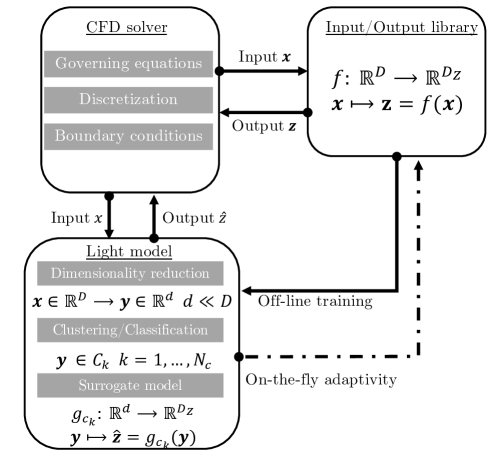
Figure 2: General schematic of the model training and coupling to replace any expensive Input/Output library.

It should be noted that this strategy is also applicable to flows in thermal non-equilibrium, where the internal energy modes are out of equilibrium with the translational energy of the flow [munafo2015modeling]. Since the additional source terms modeling the energy exchange in the internal energy equation(s) are modeled as a function of the local thermodynamic state vector as well, they can be added to the outputs and a surrogate can be constructed accordingly. This endeavor however lies outside of the scope of the current study and will be pursued as a subject of a future work. In the future, on-the-fly adaptivity will also be added to the algorithm to allow the model to learn new states as the simulation is advanced in time. This capability will help tackle more challenging and unsteady flow problems, while alleviating the need for a complete training set which may not always be available. Hence, the final intended use of the model will be as follows: (i) a preliminary laminar simulation will warm-start the training of the algorithm. (ii) as more flow features are added (such as instabilities), the model will learn adaptively the remaining “new” thermodynamics states pertaining to the new unsteady features. Following this procedure, the dynamics will be obtained at a lower CPU cost.

II.1 Training

The algorithm is trained using the simulation of an adiabatic Mach-10 boundary layer in chemical non-equilibrium, thoroughly described in LABEL:simu. The gas considered is a five-species air model ${\lx@glossaries@gls@link{roman}{speciesset}{\leavevmode\mathcal{S}}}={N_{2},O_{2},NO,N,O}$ with five reactions. The computational code solves the compressible reactive Navier-Stokes equations, where the kinetic parameters are computed by coupling with Mutation++ [Scoggins2020]. The input thermodynamic state vector $\tilde{\textbf{q}}_{\rm{th}}$ is composed of density $\rho$, internal energy $\rho e$ and the mixture partial densities $\rho_{s},s\in{\lx@glossaries@gls@link{roman}{speciesset}{\leavevmode\mathcal{S}}}$. The outputs of the library fall within three categories: thermodynamic properties (pressure $p$, temperature $T$, species specific enthalpies $h_{s},s\in{\lx@glossaries@gls@link{roman}{speciesset}{\leavevmode\mathcal{S}}}$), transport properties (viscosity $\mu$, thermal conductivity $\kappa$, diffusion coefficients $D_{s},s\in{\lx@glossaries@gls@link{roman}{speciesset}{\leavevmode\mathcal{S}}}$) and chemical kinetics source term $\dot{\omega}_{s},s\in{\lx@glossaries@gls@link{roman}{speciesset}{\leavevmode\mathcal{S}}}$. More details concerning the governing equations and the thermo-chemical model can be found in Section III.

II.1.1 Data collection

To train the model, $N$ thermodynamic state vectors $\tilde{\textbf{q}}_{\rm{th}}$ are randomly sampled on the grid of a previously converged simulation in chemical non-equilibrium and concatenated into the input vector $\tilde{\mathbf{X}}\in\mathbb{R}^{N\times D}$. The corresponding outputs from the library are collected and concatenated into the output vector $\tilde{\mathbf{Z}}\in\mathbb{R}^{N\times D_{Z}}$. Fig. 3 shows the numerical range of selected output variables along each input, normalized between $0$ and $1$ with a minimum-maximum scaling

$$\mathbf{X}=\frac{\tilde{\mathbf{X}}-\tilde{\mathbf{X}}_{min}}{\tilde{\mathbf{X}}_{max}-\tilde{\mathbf{X}}_{min}},\quad\quad\mathbf{Z}=\frac{\tilde{\mathbf{Z}}-\tilde{\mathbf{Z}}_{min}}{\tilde{\mathbf{Z}}_{max}-\tilde{\mathbf{Z}}_{min}}.$$ (2)

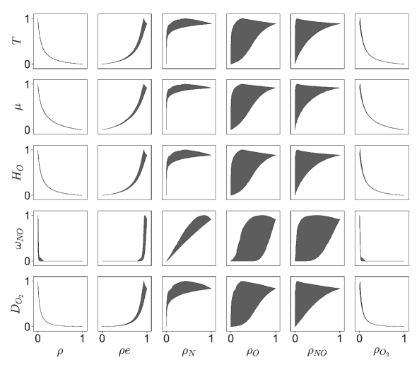
Figure 3: Numerical range of selected Mutation++ outputs $\mathbf{Z}$ (vertical) with respect to the inputs $\mathbf{X}$ (horizontal).

Taking dynamic viscosity $\mu$, for example, it shows a strong dependency on density $\rho$ and internal energy $\rho e$ but a low variation with respect to the radicals’ partial densities $\rho_{O}$, $\rho_{N}$ and $\rho_{NO}$. The same observations can be made for all other outputs. Hence, the variation of the function $\tilde{f}$ with respect to the inputs can be accurately represented on a low-dimensional subspace of the inputs. This motivates the first step of the algorithm, namely, dimensionality reduction.

II.1.2 Dimensionality reduction

The goal of this section is to find an effective algorithm for dimensionality reduction of the input space in order to construct a mapping between its reduced-order representation and the output of the library

$$\hat{\mathbf{Z}}=g(\mathbf{Y}),$$ (3)

where $g$ is the approximation of the scaled library $f$ in the low-dimensional subspace of the inputs, $\mathbf{Y}$ is the reduced-order representation of an input $\mathbf{X}$ and $\hat{\mathbf{Z}}$ the prediction of the model. The benefit of this first pre-processing step is to maintain high accuracy of the surrogate model, while decreasing the overall cost of construction and evaluation. In fact, constructing a response surface faces the well-known curse of dimensionality; as the number of input dimensions increases, the cost of constructing an accurate surface increases exponentially. This approach was proven successful in [bouhlel2016] where PLS was used in tandem with kriging to reduce the dimension of the input space.

II.1.2.1 Principal component analysis

The most common technique for dimensionality reduction of a dataset $\mathbf{X}\in\mathbb{R}^{N\times D}$ in high dimensions is principal component analysis PCA (see eg. [shlens2014]). The principal components of $\mathbf{X}$ are found through the eigenvalue decomposition of the covariance matrix of the data. The dataset $\mathbf{X}$ is then projected onto $d<D$ leading eigenvectors (or principal components) of the covariance matrix, resulting in a low-dimensional representation $\mathbf{Y}\in\mathbb{R}^{N\times d}$ of the original dataset. However, depending on the shape of the manifold, the variations of the output variables with respect to the low-dimensional sub-space may not be properly preserved, which is the case presented in Fig. 4a with points of high and low temperature projected onto similar locations. This example illustrates the limitations of PCA for dimensionality reduction of a dataset constrained to a nonlinear manifold.

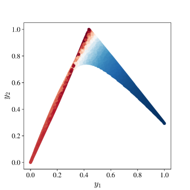
(a)

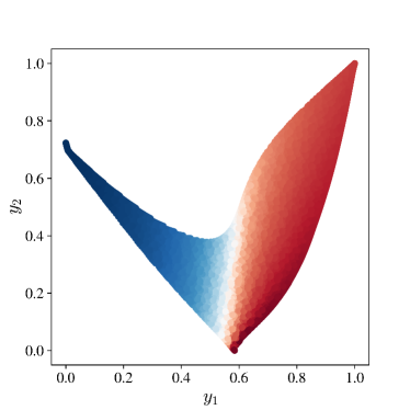
(b)

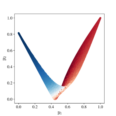
(c)

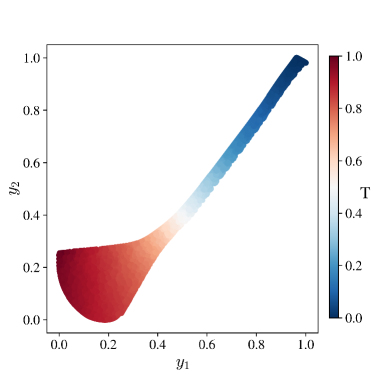
(d)

Figure 4: Low-dimensional representation $Y\in\mathbb{R}^{N\times d}$ ($d=2$) of $X\in\mathbb{R}^{N\times D}$, colored by temperature $T$. Obtained with (a) PCA (b) AE (c) PLS (d) IO-E.

II.1.2.2 Auto-encoders

Nonlinear dimensionality reduction via auto-encoders (AE) typically have a higher compression rate than linear techniques. An auto-encoder is a parametric model (i.e. a deep neural network with an activation function $\sigma$) that embeds the input dataset $\mathbf{X}\in\mathbb{R}^{N\times D}$ into a low-dimensional representation $\mathbf{Y}\in\mathbb{R}^{N\times d}$ through an encoder function $\mathbf{E}$. The low-dimensional representation is then decoded back to the input space with the decoder function $\mathbf{D}$, producing a reconstruction of the input $\widehat{\mathbf{X}}\in\mathbb{R}^{N\times D}$.

$$\begin{array}[]{l}\mathbf{Y}=\mathbf{E}(\mathbf{X})\\ \hat{\mathbf{X}}=\mathbf{D}(\mathbf{Y})\end{array}$$ (4)

The weights of the two networks $\mathbf{E}$ and $\mathbf{D}$ can be trained using back-propagation of the $L_{2}$ error $\lVert\mathbf{X}-\widehat{\mathbf{X}}\rVert_{2}$ through the network. If the activation function is selected as the identity (i.e $\sigma(\mathbf{x})=\mathbf{x}$), the auto-encoder is linear and unbiased

$$\begin{array}[]{l}\mathbf{E}=W_{E}\\ \mathbf{D}=W_{D}\end{array}$$ (5)

where $W_{E}$ and $W_{D}$ are the weights matrices of the encoder and decoder, respectively. These optimal weights can be found through PCA. In fact, the linear latent space of dimension $d$ of the encoder will span the same sub-space as the top $d$ PCA singular vectors. The equivalence between the two techniques was first shown by Baldi & Hornik [baldi1989neural]. Correspondingly, a two-layered nonlinear auto-encoder can be mathematically described as follows

$$\begin{array}[]{l}\mathbf{Y}=W_{E,2}\sigma(W_{E,1}\mathbf{X}+\mathbf{b_{E,1}})+\mathbf{b_{E,2}}\\ \hat{\mathbf{X}}=W_{D,2}\sigma(W_{D,1}\mathbf{Y}+\mathbf{b_{D,1}})+\mathbf{b_{D,2}}\end{array}$$ (6)

where $\sigma$ is a nonlinear activation function, $W_{E,1}\in\mathbb{R}^{H\times D},W_{E,2}\in\mathbb{R}^{d\times H}$ are the weights matrices of the first and second layer of the encoder with respective biases $\mathbf{b_{E,1}}\in\mathbb{R}^{H}$ and $\mathbf{b_{E,2}}\in\mathbb{R}^{d}$. $H$ denotes the dimension of the hidden layer. The matrices and bias vectors of the decoder have transposed dimensions. This corresponds to the minimal architecture (i.e. with one hidden nonlinear layer and an output linear layer) requested by the universal approximation theorem [cybenko1989approximation]. However, more hidden layers can be considered. Fig. 4b shows the manifold unrolled in two dimensions with an auto-encoder, colored by the magnitude of the temperature, an output of the library. The AE outperforms PCA by preserving the local structure and preventing points at different thermodynamic states (i.e different temperatures) to be projected onto the same location. However, the highest temperature zone is concentrated in a thin layer adjacent to the lower temperature area. This will result in strong and unphysical gradients of the surrogate model within this region.

II.1.2.3 Partial least-squares

Since our interest lies in reducing the dimensionality of the input to construct a reduced-order surrogate model of the input/output relations, it is useful to entangle the input into a low-dimensional space that best reconstructs the outputs. In analogy to PCA finding dependencies between the inputs, partial least-squares (PLS) finds a basis of the input space that optimally accounts for features in the output space. It has been used to construct surrogate models aimed at reducing the dimensions of the input space (see [bouhlel2016]). Different variants of PLS now exist, using either a singular value decomposition (PLS-SVD) or iterative algorithms (such as PLS-W2A in [wegelin2000survey]). While it has been shown that in cases where the dimension of the latent space is strictly greater than one, PLS-SVD differs from PLS-W2A and its variant PLS2, no major differences in the resulting latent space were observed. The results of PLS-SVD are presented here to highlight the similarity to PCA. Given the input $\mathbf{X}$ and output vectors $\mathbf{Z}$, the PLS-SVD algorithm [wegelin2000survey] determines

$$\mathbf{X}^{T}\mathbf{Z}=\mathbf{U\Sigma V}^{T}.$$ (7)

Similar to PCA, the projection of the input is then obtained by projecting onto the $d<D$ top left singular vectors

$$\mathbf{Y}=\mathbf{X}\overline{\mathbf{U}}$$ (8)

where $\overline{\mathbf{U}}\in\mathbb{R}^{D\times d}$ is the truncated left-singular matrix. Fig. 4c shows the training set projected onto the two-dimensional basis generated with PLS. As expected, adding the output information in the computation improves the output’s representation in the reduced-order input basis compared to PCA. However, an artificial discontinuity is created near the high-gradient region that was not present in Fig. 4b. This highlights the lower compression rate of linear techniques compared to nonlinear ones.

II.1.2.4 Input/output-encoders

The strategy adopted here is therefore a nonlinear dimensionality reduction of the input data using input/ouput-encoders (IO-E), a modified version of auto-encoders (AE) adapted to input/ouput relations. To that end, the decoder architecture is modified to best reconstruct the output of the library $\mathbf{Z}\in\mathbb{R}^{N\times D_{Z}}$ as

$$\widehat{\mathbf{Z}}=W_{D,2}\sigma(W_{D,1}\mathbf{Y}+\mathbf{b_{D,1}})+\mathbf{b_{D,2}}$$ (9)

where the weight matrices are now $W_{D,1}\in\mathbb{R}^{H_{D}\times d},W_{D,2}\in\mathbb{R}^{D_{Z}\times H_{D}}$ with respective biases $\mathbf{b_{D,1}}\in\mathbb{R}^{H_{D}}$ and $\mathbf{b_{D,2}}\in\mathbb{R}^{D_{Z}}$. $H_{D}$ now represents the hidden dimension of the decoder. The resulting network is then trained via back-propagation of the reconstruction error based on the output $\lVert\mathbf{Z}-\widehat{\mathbf{Z}}\rVert_{2}$. The input/output-encoder (IO-E) architecture is illustrated in Fig. 5.

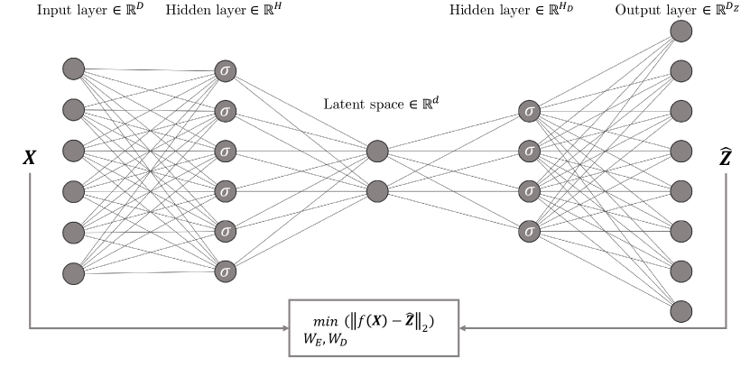
Figure 5: Schematic of the input/output-encoder architecture proposed. An input sample X is passed through the encoder network to generate a low-dimensional representation Y. Y is decoded back to predict the library output $\widehat{\textbf{Z}}$. At each training step, the $L_{2}$ loss $\lVert\mathbf{Z}-\widehat{\mathbf{Z}}\rVert_{2}$ between the library and the network prediction is calculcated and backpropagated until convergence of the encoder and decoder weights, $W_{E}$ and $W_{D}$, respectively, is reached.

Fig. 4d shows the equivalent manifold using the IO-E architecture, with the same number of hidden dimensions. The IO-E architecture outperforms all other techniques as the high-temperature region is now projected onto its own properly defined zone with smooth variations. This feature will have a marked impact on the performance of the library when linked to the solver. It is worth noting that the decoder part of the IO-E could be used directly to predict the output of the library. However, we will see in LABEL:mode_acc that the accuracy of the full IO-E would not optimal in this case. This motivates the use of clustering and radial basis functions, as described next.

II.1.3 Community clustering

In the second step of the algorithm, we seek to discover clusters within our data. In our present context, a cluster represents a subset of data that shares similar thermodynamic features. These feature classification will then be useful in constructing a dedicated surrogate surface of the low-dimensional input manifold. To this end, Newman’s spectral algorithm for community detection in a network [newman2006] is used. A clear advantage of Newman’s algorithm is that the number of clusters is not defined a priori, in contrast to more common clustering techniques (e.g. k-means). The number of clusters is instead the result of a maximization procedure performed on the modularity $Q$ of the network. In other words, the number of thermodynamic clusters in the flow are determined only from the data and is not based on a priori knowledge of the user. This knowledge might be even impossible to come by in complex, unsteady hypersonic flows subjected to shocks.

Following this approach, the Euclidean distance matrix $\Delta$ of the dataset in low-dimensional space is computed

$$\Delta_{ij}=\lVert\mathbf{Y}_{i}-\mathbf{Y}_{j}\rVert^{2}\quad\text{for}\quad(\mathbf{Y}_{i},\mathbf{Y}_{j})\in\mathbf{Y}^{2}.$$ (10)

The dataset is subsequently recast into an undirected network with a binary adjacency matrix $A$, constructed as

$$A_{ij}=\left\{\begin{array}[]{lcl}1&\phantom{1234}&\mbox{if}~{}\Delta_{ij}<\epsilon,\\ 0&&\mbox{otherwise.}\end{array}\right.$$ (11)

Two points are connected with an edge if their Euclidean distance is below a certain threshold $\epsilon$. This threshold is usually chosen as a fraction of the mean of the distance matrix $\Delta$. The influence of the threshold $\epsilon$ on the number of clusters will be investigated in LABEL:cluster-training.

Finally, the dataset is progressively split into two communities until the modularity, $Q$, is maximized. The modularity is defined as the proportion of edges contained within a community over the same proportion for a random reference network. Let $k_{i}$ be the number of edges pointing towards the data point numbered $i$, and $m$ the total number of connections within the network. Then, the probability of having an edge between $i$ and $j$ in the random reference network is $k_{i}k_{j}/m$. Hence, the modularity $Q$ is defined as,

$$Q=\frac{1}{m}\sum_{ij}\left(A_{ij}-\frac{k_{i}k_{j}}{m}\right)\delta_{c_{i},c_{j}},$$ (12)

where $\delta_{c_{i},c_{j}}$ is the Kronecker delta for the communities of $i$ and $j$. For instance, $\delta_{c_{i},c_{j}}=1$ only when $i$ and $j$ belong to the same community. By defining a vector s where $s_{i}=1$ if vertex $i$ belongs to the first group, and $s_{i}=-1$ otherwise, we can reformulate

$$Q=\frac{1}{2m}\sum_{ij}\left(A_{ij}-\frac{k_{i}k_{j}}{m}\right)(s_{i}s_{j}+1)=\frac{1}{2m}\mathbf{s^{T}}B\mathbf{s},$$ (13)

where the modularity matrix $B$ is given as,

$$B_{ij}=A_{ij}-\frac{k_{i}k_{j}}{m}.$$ (14)

Since the graph is undirected, the modularity matrix $B$ is symmetric and the modularity $Q$ represents a Rayleigh quotient for matrix $B$. In order to maximize $Q$, we need to choose a vector $s$ that is parallel to the principal eigenvector (corresponding to the largest eigenvalue) of $B$, v, which can be achieved by setting $s_{i}=1$ if $v_{i}>0$ and $s_{i}=-1$ if $v_{i}<0$. In order to partition the graph into more than two communities, this algorithm is repeated until the modularity of each subgraph can no longer be increased. A thorough descripion of the full algorithm can be found in [newman2006].

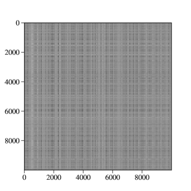
(a)

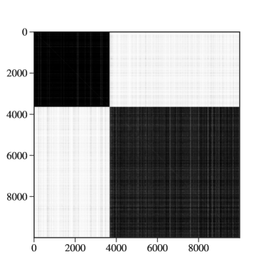
(b)

Figure 6: Demonstration of the Newman algorithm. (a) Original distance matrix $\Delta$ of dataset $\mathbf{Y}$. (b) Restored communities from running Newman’s algorithm on $A$, showing two distinct clusters

Fig. 6a shows the application of the clustering algorithm to the boundary layer data. The distance matrix $\Delta$ is constructed on $\mathbf{Y}$. After running the algorithm on the subsequent adjacency matrix $A$, two distinct clusters are identified, highlighted by the low distance between the points within a cluster in Fig. 6b.

II.1.4 Surrogate model construction

Finally, a surrogate surface is computed on the scattered low-dimensional points of each cluster. Many algorithms can be used to that end, such as kriging [kleijnen2009kriging, bouhlel2016], artificial neural networks [sun2019review], or radial basis functions [broomhead1988radial, powell1992rbf, buhmann2000radial]. In the application of interest to this work, radial basis functions (RBF) provided the best trade-off between performance and accuracy, as well as an easy training step. In fact, the optimal weights of a RBF can be obtained through the solution of a linear system. However, it should be noted that our choice is not definitive and can be easily changed.

Given a set of $N_{R}$ input points $\textbf{x}_{1},...,\textbf{x}_{N_{R}}\in\mathbb{R}^{d}$ and the function value at these points $f(\textbf{x}_{1}),...,f(\textbf{x}_{N_{R}})$ the radial basis function (RBF) interpolant $g$ is given by

$$g(\phi,x)=\sum_{i=1}^{N_{R}}\lambda_{i}\phi(\lVert\textbf{x}-\textbf{x}_{i}\rVert)$$ (15)

where $\phi$ is the kernel function whose value depends on the distance $r=\lVert\textbf{x}-\textbf{x}_{i}\rVert$ between the evaluation point x and the center $\textbf{x}_{i}$ of the RBF. In this study, the thin-plate spline kernel [wood2003thin] was used, i.e.,

$$\phi(r)=r^{2}log(r).$$ (16)

With this particular kernel, the kernel matrix is only conditionally positive definite. To ensure a unique solution for the interpolation weights, the system is augmented by a polynomial $p\in\Pi^{d}_{m}$ (space of polynomials of $d$ variables and degree up to $m$) to the right hand side of Eq. 15 [buhmann2000radial], resulting in

$$g(x)=\sum_{i=1}^{N_{R}}\lambda_{i}\phi(\lVert x-x_{i}\rVert)+p(x).$$ (17)

The extra degrees of freedom are accounted for by enforcing orthogonality of the coefficients with respect to the polynomial space as

$$\sum_{i=1}^{N_{R}}\lambda_{i}r(\textbf{x})=0,r\in\Pi_{m}^{d}.$$ (18)

Finally, the polynomial coefficients $\textbf{c}=[c_{1},...,c_{d+1}]^{T}$ and the RBF coefficients $\bm{\Lambda}=[\lambda_{1},...,\lambda_{N_{R}}]^{T}$ are found through the solution of the following linear system

$$\begin{bmatrix}\mathbf{\Phi}&\mathbf{P}\\ \mathbf{P}^{T}&0\end{bmatrix}\begin{bmatrix}\bm{\Lambda}\\ \mathbf{c}\end{bmatrix}=\begin{bmatrix}\mathbf{f}\\ 0^{d+1}\end{bmatrix}$$ (19)

where $\textbf{P}_{i}=[1,x_{i},...,x_{i}^{d}]$ for $i\in[1,N_{R}]$ is the polynomial matrix, and $\textbf{f}=[f(\textbf{x}_{1}),...,f(\textbf{x}_{N_{R}})]$ denotes the vector containing the function values at the RBF centers.
Due to the large size of the training set, using one cluster center per training point (i.e. $N_{R}=N=O(10^{5})$) will likely result in overfitting and prohibitive computational cost [schwenker2001three]. Following the recommendations in [schwenker2001three], the interpolant is constructed in two steps. First, the k-means algorithm with $N_{R}\ll N$ clusters is applied on the concatenation of the input and output vector $(\mathbf{X},\mathbf{Z})\in\mathbb{R}^{N\times(D+D_{Z})}$. The addition of the output vector results in a low within-cluster variance of the outputs and will ultimately improve the surrogate model. The $N_{R}$ centroids obtained with k-means, $\textbf{x}^{c}$, are sent to the library to compute the function value vector f. Simultaneously, they are encoded in the low-dimensional space to obtain the $N_{R}$ cluster centers that will be used to train the RBF $\textbf{y}^{c}_{1},...,\textbf{y}^{c}_{N_{R}}\in\mathbb{R}^{d}$. Fig. 7 shows the resulting tesselation in the embedded space after applying the k-means algorithm with $N_{R}=250$. The influence of the number of RBF centers on the quality of the surrogate model will be assessed in LABEL:rbf-training.

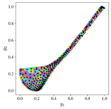
Figure 7: Tesselation of the low-dimensional space after applying the k-means algorithm with $N_{R}=250$ on the concatenation of the input $\textbf{X}\in\mathbb{R}^{N\times D}$ and output $\textbf{Z}\in\mathbb{R}^{N\times D_{Z}}$ vectors. Black stars represent the cluster centroids’ low-dimensional representation $\textbf{y}^{c}_{1},...,\textbf{y}^{c}_{N_{R}}$.

Following this approach, a single interpolant, $g_{c_{k}}$, is constructed for each cluster, $c_{k}$; in other words, $g_{c_{k}}$ is the approximation of the scaled library function $f$ on the low-dimensional subspace corresponding to cluster $c_{k}$. The advantage of having one interpolant per cluster is twofold. First, it allows the surrogate model to best fit a region with a given dynamics of the high-dimensional function, especially in the presence of discontinuities, similar to the approach of Bettebghor et al. [bettebghor2011]. Secondly, as the surrogate model spans a smaller range of input parameters, less centers are required to capture the given dynamics accurately, resulting in a lighter model with faster evaluation time. To enforce continuity of the surrogate surface near the cluster boundaries, the nearest centroids that do not belong to the considered cluster are added to its training set.

II.2 Coupling to the solver

Once the model is trained, we can replace the calls of the solver to the look-up library with the new lighter model. New points have to go through three steps: (i) Out-of-sample dimensionality reduction, (ii) classification, and (iii) interpolation. These three steps will be described in the following. Let $\mathbf{X}^{t}\in\mathbb{R}^{N_{t}\times D}$ denote the stack of all new points.

II.2.1 Out-of-sample encoding

The low-dimensional representation of $\mathbf{X}^{t}$ (after proper scaling of $\tilde{\mathbf{X}}^{t}$) is straightforward. Indeed, the point is simply fed to the encoder portion of the input/output-encoder

$$\mathbf{Y}^{t}=W_{E,2}\sigma(W_{E,1}\mathbf{X}^{t}+\mathbf{b_{E,1}})+\mathbf{b_{E,2}}.$$ (20)

This results in a fast and inexpensive encoding of the new out-of-sample points. In fact, the time complexity of the encoding step is $O(H\times C_{ac}\times L\times N_{t})$, where $H$ is the maximum number of neurons in a layer, $C_{ac}$ is the complexity of the activation function and $L$ is the number of layers in the encoder step of the input/output-encoder.

II.2.2 Classification

The next step is to determine to which community the new state $\mathbf{Y}^{t}$ belongs. To this end, after applying Newman’s algorithm, a random forest classifier is trained on the resulting clusters. A random forest classifier, formally proposed by Breiman [breiman2001random], is a collection of $n_{tree}$ tree-based classifiers, ${h(\textbf{x},\Phi_{k}),k=1,...,n_{tree}}$, where $\Phi_{k}$ are identically distributed random vectors. Each tree votes for the most likely class of input vector $\textbf{x},$ and the majority wins. Fig. 8 shows the confusion matrix $C$ of the classifier trained on the two clusters obtained above with $n_{tree}=20$. The clusters of the embedded new points $\mathbf{Y}^{t}$, not seen during the training-phase of the classifier, are predicted and compared to the true clusters (given by Newman’s algorithm). The off-diagonal values count the number of points that are assigned to the wrong cluster. All off-diagonal values are zero, demonstrating the ability of the classifier to correctly predict the community of an out-of-sample point.

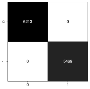
Figure 8: Confusion matrix $C$ of the random forest classifier ($n_{tree}=20$), tested on unseen data points during training. $C_{ij}$ is the number of points belonging to cluster $c_{j}$ predicted to be in cluster $c_{i}$.

The time complexity of the induction time of the classifier is $O(n_{tree}\times N_{t}log(N_{t}))$ (see the book by Witten, Frank and Hall [frank2004data] for a demonstration), where $n_{tree}$ is the number of decision trees in the random forest. The logarithmic term accounts for the worst case scenario for the maximum depth of each tree. However, the maximum depth is usually set to a smaller value, resulting in a complexity of $O(n_{tree}\times depth\times N_{t})$, which results in relatively fast classification times.

II.2.3 Interpolation

Finally, once $\mathbf{Y}^{t}$ has been found to belong to cluster $c_{k}$, the corresponding RBF $g_{c_{k}}$ is called to evaluate the thermochemical properties $\widehat{\mathbf{Z}}^{t}$ of the mixture at that state $\mathbf{X}^{t}$,

$$\widehat{\mathbf{Z}}^{t}=g_{c_{k}}(\mathbf{Y}^{t})=\sum_{i=1}^{N_{R}}\lambda_{i}\phi(\mathbf{Y}^{t}-\mathbf{Y}^{c}_{i}).$$ (21)

The hat denotes the predicted value by the reduced library, as opposed to the true value that would have been given by the target library, $\mathbf{Z}^{t}$. Finally, these properties are re-scaled according to

$$\tilde{\widehat{\mathbf{Z}}}^{t}=\widehat{\mathbf{Z}}^{t}*(\tilde{\mathbf{\mathbf{Z}}}_{max}-\tilde{\mathbf{Z}}_{min})+\tilde{\mathbf{Z}}_{min}$$ (22)

and passed back to the flow solver.

The time complexity of each surrogate model is given by $O(C_{RBF}\times N_{t}\times N_{R}\times d)$, where $C_{RBF}$ is the complexity of the kernel function. The time limiting part of the RBF interpolation is the calculation of the distance matrix that scales with $O(N_{t}\times N_{R}\times d)$. Hence, using a relatively small number $N_{R}$ of RBF centers, compared to $N_{t},$ will greatly improve the performance of the surrogate model. It should be noted that the dimensionality reduction directly contributes to the added performance of the surrogate model as $d<D$.

II.2.4 Global performance

The time complexity of the whole algorithm can be recovered by adding the time complexity of each of the three steps. Hence, the total time complexity of the algorithm can be written as $O(C_{ML}N)$, where $C_{ML}=O(HC_{ac}L+n_{tree}depth+dN_{R}C_{RBF})$.

III Application to hypersonic flows in chemical non-equilibrium

In this section, the general equations governing hypersonic flows in chemical non-equilibrium are first recalled, followed by a brief description of the numerical framework used to solve these equations. Then, the two benchmark cases, a Mach-10 adiabatic laminar boundary layer in chemical non-equilibrium, initially studied by Marxen et al [Marxen2013, Marxen2014], and a Mach-5.92 shock wave boundary layer interaction are presented.

III.1 Governing conservation equations

The nondimensional Navier-Stokes equations for a mixture of multiple species $\mathcal{S}$  are presented in Eqs. 23 to 26.

$$\frac{\partial\density}{\partial{\lx@glossaries@gls@link{roman}{timevar}{\leavevmode t}}} +\mathbf{\nabla}\cdot\left(\density{\lx@glossaries@gls@link{roman}{velocity}{\leavevmode\mathbf{u}}}\right) =0$$ (23)

$$\left\{\vphantom{\frac{1}{1}}\right. \frac{\partial{\lx@glossaries@gls@link{greek}{densityspecies}{\leavevmode\density_{\lx@glossaries@gls@link{subsc}{speciess}{\leavevmode\mathrm{s}}}}}}{\partial{\lx@glossaries@gls@link{roman}{timevar}{\leavevmode t}}} +\mathbf{\nabla}\cdot\left({\lx@glossaries@gls@link{greek}{densityspecies}{\leavevmode\density_{\lx@glossaries@gls@link{subsc}{speciess}{\leavevmode\mathrm{s}}}}}{\lx@glossaries@gls@link{roman}{velocity}{\leavevmode\mathbf{u}}}+{\lx@glossaries@gls@link{greek}{densityspecies}{\leavevmode\density_{\lx@glossaries@gls@link{subsc}{speciess}{\leavevmode\mathrm{s}}}}}{\lx@glossaries@gls@link{roman}{diffvelocity}{\leavevmode\mathbf{V}_{\lx@glossaries@gls@link{subsc}{speciess}{\leavevmode\mathrm{s}}}}}\right) ={\lx@glossaries@gls@link{greek}{massprod}{\leavevmode{\dot{\omega}}_{\lx@glossaries@gls@link{subsc}{speciess}{\leavevmode\mathrm{s}}}}}\left.\vphantom{\frac{1}{1}}\right\}\;,\;\forall\;{\lx@glossaries@gls@link{subsc}{speciess}{\leavevmode\mathrm{s}}}\in{\lx@glossaries@gls@link{roman}{speciesset}{\leavevmode\mathcal{S}}}$$ (24)

$$\frac{\partial\density{\lx@glossaries@gls@link{roman}{velocity}{\leavevmode\mathbf{u}}}}{\partial{\lx@glossaries@gls@link{roman}{timevar}{\leavevmode t}}} +\mathbf{\nabla}\cdot\left(\density{\lx@glossaries@gls@link{roman}{velocity}{\leavevmode\mathbf{u}}}\otimes{\lx@glossaries@gls@link{roman}{velocity}{\leavevmode\mathbf{u}}}\right) =-\mathbf{\nabla}{\lx@glossaries@gls@link{roman}{pressure}{\leavevmode p}}+\mathbf{\nabla}\cdot{\lx@glossaries@gls@link{greek}{viscstresstensor}{\leavevmode\mathrm{\uptau}}}$$ (25)

$$\frac{\partial\density{\lx@glossaries@gls@link{roman}{totale}{\leavevmode{\lx@glossaries@gls@link{roman}{internale}{\leavevmode e}}_{\lx@glossaries@gls@link{subsc}{totalnot}{\leavevmode\mathrm{0}}}}}}{\partial{\lx@glossaries@gls@link{roman}{timevar}{\leavevmode t}}} +\mathbf{\nabla}\cdot\left(\density{\lx@glossaries@gls@link{roman}{totalh}{\leavevmode{\lx@glossaries@gls@link{roman}{internalh}{\leavevmode h}}_{\lx@glossaries@gls@link{subsc}{totalnot}{\leavevmode\mathrm{0}}}}}{\lx@glossaries@gls@link{roman}{velocity}{\leavevmode\mathbf{u}}}\right) =\mathbf{\nabla}\cdot\left({\lx@glossaries@gls@link{greek}{viscstresstensor}{\leavevmode\mathrm{\uptau}}}\cdot{\lx@glossaries@gls@link{roman}{velocity}{\leavevmode\mathbf{u}}}\right)-\mathbf{\nabla}\cdot{\lx@glossaries@gls@link{roman}{heatflux}{\leavevmode\mathbf{q}}}$$ (26)

Equation 23 is the continuity equation, describing mass conservation in the system. Equation 24 corresponds to the set of mass conservation equations for each species, with the net production rate terms, ${\dot{\omega}}_{\lx@glossaries@gls@link{subsc}{speciess}{\leavevmode\mathrm{s}}}$, appearing on their right-hand side. In order to ensure global mass conservation, in the case of a finite-rate reacting mixture with a varying composition, Eq. 23 needs to be solved together with Eq. 24 for all but one species. The omitted species is selected based on numerical considerations, avoiding species with the smallest concentrations.

The nondimensional quantities are the time, $t$, the density, , the velocity, $\mathbf{u}$, the pressure, $p$, the stress tensor, $\mathrm{\uptau}$, the total energy, ${\lx@glossaries@gls@link{roman}{internale}{\leavevmode e}}_{\lx@glossaries@gls@link{subsc}{totalnot}{\leavevmode\mathrm{0}}}$, the total enthalpy, ${\lx@glossaries@gls@link{roman}{internalh}{\leavevmode h}}_{\lx@glossaries@gls@link{subsc}{totalnot}{\leavevmode\mathrm{0}}}$, the heat flux, $\mathbf{q}$, as well as, the partial density, $\density_{\lx@glossaries@gls@link{subsc}{speciess}{\leavevmode\mathrm{s}}}$, the net mass production rate, ${\dot{\omega}}_{\lx@glossaries@gls@link{subsc}{speciess}{\leavevmode\mathrm{s}}}$, and the diffusion velocity, $\mathbf{V}_{\lx@glossaries@gls@link{subsc}{speciess}{\leavevmode\mathrm{s}}}$, for the species $\mathrm{s}$. More details regarding the derivation of the equations and the validity of our invoked assumptions are provided in [Anderson2019, Gnoffo1989, Josyula2015_equations]. There are ${\lx@glossaries@gls@link{roman}{numspecies}{\leavevmode N_{\lx@glossaries@gls@link{subsc}{speciess}{\leavevmode\mathrm{s}}}}}-1$ conservation equations for the species, so the total problem involves ${\lx@glossaries@gls@link{roman}{numspecies}{\leavevmode N_{\lx@glossaries@gls@link{subsc}{speciess}{\leavevmode\mathrm{s}}}}}+4$ equations. The stress tensor, $\mathrm{\uptau}$, and the heat flux, $\mathbf{q}$, are computed as

(27)