Abstract

A method is advanced allowing for fast regulation of magnetization direction in magnetic nanosystems. The examples of such systems are polarized nanostructures, magnetic nanomolecules, magnetic nanoclusters, magnetic graphene, dipolar and spinor trapped atoms, and quantum dots. The emphasis in the paper is on magnetic nanomolecules and nanoclusters. The method is based on two principal contrivances: First, the magnetic sample is placed inside a coil of a resonant electric circuit creating a feedback field, and second, there is an external magnetic field that can be varied so that to dynamically support the resonance between the Zeeman frequency of the sample and the natural frequency of the circuit during the motion of the sample magnetization. This method can find applications in the production of memory devices and other spintronic appliances.

1 Introduction

In the problem of regulating spin dynamics, there are two principal challenges contradicting each other. First, it is necessary to possess the ability of keeping fixed the device magnetization for sufficiently long time. And second, one has to have the capability of quickly varying the magnetization direction at any required time. The possibility of keeping fixed the magnetization direction, as such, is not a difficult task that can be easily realized by using the materials enjoying strong magnetic anisotropy. The well known examples of materials with strong magnetic anisotropy are magnetic nanomolecules [1, 2, 3, 4, 5, 6, 7, 8, 9, 10, 11] and magnetic nanoclusters [12, 13, 14, 15, 16]. These materials can possess large spins and strong magnetic anisotropy keeping, at low temperature, below the blocking temperature, the sample magnetization frozen. At the same time, the strong magnetic anisotropy prevents the realization of fast magnetization reversal because of two reasons. First, as will be shown below, magnetic anisotropy induces the dynamic variation of the effective Zeeman frequency which cannot be compensated by a constant magnetic field, and second, even inverting the external magnetic field, the sample spin cannot be quickly reversed because of the strong magnetic anisotropy. Thus the dilemma arises: For fixing during the required long time the magnetization direction, one needs a rather strong magnetic anisotropy; however the latter does not allow for fast magnetization reversal.

In the present paper, we advance an original way out of the above dilemma. We keep in mind the materials enjoying magnetic anisotropy sufficient for fixing the sample magnetization. These can be magnetic nanomolecules or magnetic nanoclusters. To some extent, the consideration is applicable to dipolar and spinor trapped atoms [17, 18, 19, 20, 21, 22, 23] and to magnetic graphene (graphene with magnetic defects) [24, 25]. Quantum dots in many aspects are similar to nanomolecules [26] and also can possess magnetization [27, 28, 29, 30] that could be governed.

The method we suggest is based on two principal points. First, the considered sample is placed inside a magnetic coil of an electric circuit. Then the moving magnetization of the sample produces electric current in the circuit, which, in turn, creates a magnetic feedback field acting on the sample. An effective coupling between the circuit and the sample appears only when the circuit natural frequency is in resonance with the Zeeman frequency of the sample. However, the magnetic anisotropy, as we show, leads to the detuning of the effective Zeeman frequency from the resonance. Moreover, this detuning is dynamic, varying in time. The second pillar of the suggested method is the use of a varying external magnetic field realizing the dynamic tuning of the effective Zeeman frequency to the resonance with the circuit natural frequency. Since the tuning procedure is dynamic, the method is called the dynamic resonance tuning.

2 Magnetic nanomolecules and nanoclustres

Single-domain nanomolecules and nanoclusters are of special interest for spintronics. Due to strong exchange interactions, the spins of particles forming the nanomagnet point in the same direction thus creating a common spin and hence the common single magnetization vector. Under the action of external fields, the magnetization vector moves as a whole, which is called coherent motion. At the same time, such nanomagnets usually possess a rather strong magnetic anisotropy. The standard Hamiltonian of a nanomagnet with a spin $S$ has the form

$$\hat{H}=-\mu_{S}{\bf B}\cdot{\bf S}+\hat{H}_{A}\;,$$ (1)

where the first is the Zeeman term, $\mu_{S}=-g_{S}\mu_{B}$, $g_{S}$ is a Landé factor, $\mu_{B}$ is the Bohr magneton, and ${\bf S}$ is a spin operator. The second term describes the nanomagnet magnetic anisotropy,

$$\hat{H}_{A}=-DS_{z}^{2}+E(S_{x}^{2}-S_{y}^{2})\;,$$ (2)

with the anisotropy parameters

$$D=\frac{1}{2}\;(D_{xx}+D_{yy})-D_{zz}\;,\qquad E=\frac{1}{2}\;(D_{xx}-D_{yy})\;,$$

expressed through the dipolar tensor $D_{\alpha\beta}$ and $S_{\alpha}$ being spin-operator components.

The sample is inserted into a magnetic coil of an electric circuit producing a feedback field $H$. The coil axis is in the $x$ direction. The total magnetic field, acting on the sample,

$${\bf B}=H{\bf e}_{x}+B_{1}{\bf e}_{y}+(B_{0}+\Delta B){\bf e}_{z}\;,$$ (3)

consists of the feedback field $H$, a small anisotropy field $B_{1}$, and an external magnetic field $B_{0}+\Delta B$, with $B_{0}$ being a constant field and $\Delta B$ being a regulated part of the field. The electric circuit plays the role of a resonator. The motion of the sample magnetization creates in the circuit electric current satisfying the Kirhhoff equation. In its turn, the electric current forms the feedback magnetic field defined by the equation [31] following from the Kirhhoff equation,

$$\frac{dH}{dt}+2\gamma H+\omega^{2}\int_{0}^{t}H(t^{\prime})\;dt^{\prime}=-4\pi\eta_{res}\;\frac{dm_{x}}{dt}\;,$$ (4)

where $\gamma$ is the circuit attenuation, $\omega$, the resonator natural frequency, and $\eta_{res}\approx V/V_{res}$ is the resonator coil filling factor, $V$ being the sample volume, and $V_{res}$, the resonator coil volume. The right-hand side of the equation characterizes the electromotive force due to the moving average magnetization

$$m_{x}=\frac{\mu_{S}}{V}\;\langle\;S_{x}\;\rangle\;.$$ (5)

Writing down the Heisenberg equations of motion, we average them, looking for the dynamics of the average spin components

$$x=\frac{\langle\;S_{x}\;\rangle}{S}\;,\qquad y=\frac{\langle\;S_{y}\;\rangle}{S}\;,\qquad z=\frac{\langle\;S_{z}\;\rangle}{S}\;,$$ (6)

with $S$ being the sample spin. In the process of the averaging, we meet the combination of spins $S_{\alpha}S_{\beta}+S_{\beta}S_{\alpha}$. It would be incorrect to decouple this combination in the simple mean-field approximation, since for $S=1/2$ this combination has to be zero. The correct decoupling [32], that is exactly valid for $S=1/2$ as well as asymptotically exact for large spins, is done in the corrected mean-field approximation

$$\langle\;S_{\alpha}S_{\beta}+S_{\beta}S_{\alpha}\;\rangle=\left(2-\;\frac{1}{S}\right)\;\langle\;S_{\alpha}\;\rangle\langle\;S_{\beta}\;\rangle\;.$$ (7)

For what follows, we need to introduce several notations. We define the Zeeman frequency

$$\omega_{0}\equiv-\;\frac{\mu_{S}}{\hbar}\;B_{0}\;,$$ (8)

and the anisotropy frequencies

$$\omega_{1}\equiv-\;\frac{\mu_{S}}{\hbar}\;B_{1}\;,\qquad\omega_{D}\equiv(2S-1)\;\frac{D}{\hbar}\;,\qquad\omega_{E}\equiv(2S-1)\;\frac{E}{\hbar}\;.$$ (9)

The dimensionless anisotropy parameter is defined as

$$A\equiv\frac{\omega_{D}+\omega_{E}}{\omega_{0}}\;.$$ (10)

The dimensionless regulated field is given by the expression

$$b\equiv-\;\frac{\mu_{S}\Delta B}{\hbar\omega_{0}}\;.$$ (11)

From the evolution equations, it is seen that the coupling between the resonant circuit and the sample is characterized by the coupling rate

$$\gamma_{0}\equiv\pi\eta_{res}\;\frac{\mu_{S}^{2}S}{\hbar V}=\pi\;\frac{\mu_{S}^{2}S}{\hbar V_{res}}\;.$$ (12)

Finally, the dimensionless feedback field is denoted by

$$h\equiv-\;\frac{\mu_{S}H}{\hbar\gamma_{0}}\;.$$ (13)

Thus we come to the system of equations

$$\frac{dx}{dt}=-\omega_{S}y+\omega_{1}z\;,\qquad\frac{dy}{dt}=\omega_{S}x-\gamma_{0}hz\;,$$

$$\frac{dz}{dt}=2\omega_{E}xy-\omega_{1}x+\gamma_{0}hy\;,$$ (14)

in which the effective Zeeman frequency is

$$\omega_{S}\equiv\omega_{0}\;(1+b-Az)\;.$$ (15)

The feedback-field equation (4) becomes

$$\frac{dh}{dt}+2\gamma h+\omega^{2}\int_{0}^{t}h(t^{\prime})\;dt^{\prime}=4\;\frac{dx}{dt}\;.$$ (16)

Of course, the evolution equations are to be complemented by the initial conditions ${\bf x}(0)=\bf{x}_{0}$ for the vector ${\bf x}=\{x,y,z\}$ and for the feedback field $h(0)=h_{0}$. In what follows, we set the initial conditions as $x_{0}=y_{0}=0$, $h_{0}=0$, and $z_{0}=1$. These initial conditions correspond to the setup, when there are no alternating fields pushing the spin motion and all the following dynamics is self-organized.

3 Dynamic resonance tuning for single spins

The initial setup $s_{0}=1$ describes the sample with the spin polarization, formed by electrons, directed up, hence the magnetization directed down, while the external magnetic field $B_{0}$ is directed up. This implies that the sample is in a metastable state. The stable state corresponds to the magnetization up, hence to the spin polarization down.

Because of the strong magnetic anisotropy, the magnetization is frozen and, below the blocking temperature, it can exist in this metastable state for days and months. This is convenient for keeping the information in memory devices. However, if on needs to rewrite or erase the information, which also is an action typical of memory devices, then the frozen magnetization hinders this. Thus we confront the problem: how could we overcome the anisotropy in order to start moving the sample spin and to move it sufficiently fast?

If there would be resonance between the resonator natural frequency $\omega$ and the effective Zeeman frequency $\omega_{S}$, which is possible in the absence of the magnetic anisotropy, when $A=0$, then there would appear strong coupling between the resonator feedback field and the sample magnetization, as a result of which the magnetization could be quickly reversed at the initial time [31, 32, 33, 34, 35]. However, the effective Zeeman frequency (15) cannot be tuned to a constant resonator natural frequency $\omega$, since the effective Zeeman frequency is not a constant but a function of the polarization $z$. For instance, if $\omega$ is tuned to $\omega_{0}$, then the relative detuning

$$\frac{\omega_{S}-\omega_{0}}{\omega_{0}}=b-Az$$

varies in time and, generally, can be very large for large anisotropy parameters $A$.

Suppose, we have been keeping the magnetization fixed for a required time $\tau$, after which we need to quickly reverse it. To make the detuning small, and moreover for keeping it small during the whole process of spin reversal, we suggest to set $\omega_{0}=\omega$ and to vary the regulated field $b=b(t)$ according to the law of dynamic resonance tuning, so that

$$b(t)=\left\{\begin{array}[]{ll}0\;,{}&~{}t<\tau\\ Az_{reg}\;,{}&~{}t\geq\tau\;,\end{array}\right.$$ (19)

with $z_{reg}$ satisfying the equations

$$\frac{dx_{reg}}{dt}=-\omega_{0}y_{reg}+\omega_{1}z_{reg}\;,\qquad\frac{dy_{reg}}{dt}=\omega_{0}x_{reg}-\gamma_{0}h_{reg}z_{resg}\;,$$

$$\frac{dz_{reg}}{dt}=2\omega_{E}x_{reg}y_{reg}-\omega_{1}x_{reg}+\gamma_{0}h_{reg}y_{reg}\;,$$

$$\frac{dh_{reg}}{dt}+2\gamma h_{reg}+\omega^{2}\int_{\tau}^{t}h_{reg}(t^{\prime})\;dt^{\prime}=4\;\frac{dx_{reg}}{dt}\;.$$ (20)

The initial conditions for the latter system of equations can be taken either as ${\bf x}_{reg}(\tau)={\bf x}(\tau)$ and $h_{reg}(\tau)=h(\tau)$ or as ${\bf x}_{reg}(\tau)={\bf x}_{0}$ and $h_{reg}(\tau)=h_{0}$.

In Fig. 1, we show the process where the spin polarization is frozen, by a strong magnetic anisotropy, during the time $\tau$, after which the mechanism of the dynamic resonance tuning is switched on. Different initial conditions are compared, as explained in the Figure, demonstrating that they lead to a slight shift of the reversal process. It is also shown that if the resonance condition is not dynamic, but only the initial triggering resonance [36], when the condition $b(\tau)=Az(\tau)$ is imposed, then the reversal is not fast but possesses a long tail. Time is measured in units of $\gamma_{0}^{-1}$ and frequencies, in units of $\gamma_{0}$.

     

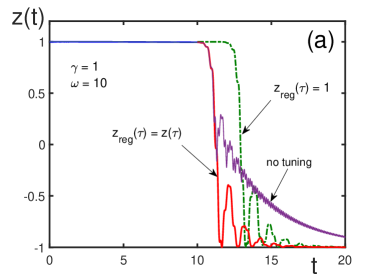
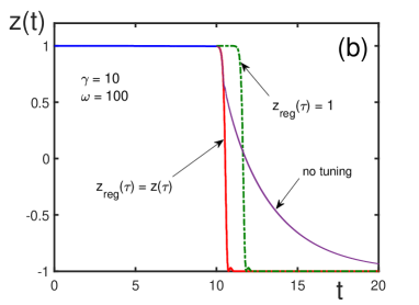
Figure 1: Spin polarization $z(t)$ of a nanocluster or nanomolecule as a function of time under dynamic resonance tuning, starting at the delay time $\tau=10$, for different initial conditions, as explained in the Figure. The anisotropy parameters are $A=1$ and $\omega_{E}=\omega_{1}=0.01$. The line with a long tail describes the process, where the dynamic resonance tuning is not used, but instead the condition of triggering resonance at the same initial time is employed. (a) $\omega=\omega_{0}=10$ and $\gamma=1$; (b) $\omega=\omega_{0}=100$ and $\gamma=10$. Time is measured in units of $\gamma_{0}^{-1}$ and frequencies, in units of $\gamma_{0}$.

In Fig. 2, the spin polarization of a nanocluster or nanomolecule is shown for dynamic resonance tuning, compared with the polarization without dynamic tuning but under the triggering resonance at the same delay time. The advantage of dynamic resonance tuning is in an ultrafast spin reversal, while the triggering resonance leads to long tails.

     

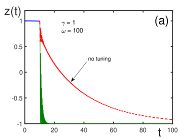
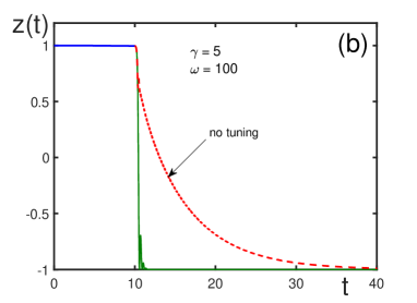
Figure 2: Spin polarization $z(t)$ of a nanocluster or nanomolecule as a function of time under dynamic resonance tuning, starting at the delay time $\tau=10$ (solid line), compared with the polarization without dynamic tuning but under the triggering resonance at the same delay time (dashed line). The anisotropy parameters are $A=1$ and $\omega_{E}=\omega_{1}=0.01$. (a) $\omega=\omega_{0}=100$ and $\gamma=1$; (b) $\omega=\omega_{0}=100$ and $\gamma=5$. The absence of dynamic tuning leads to long tails.

Figure 3 illustrates the reversal of the spin polarization of a nanocluster or nanomolecule under dynamic resonance tuning, starting at different delay times. This shows that it is possible to quickly reverse the magnetization at any required time.

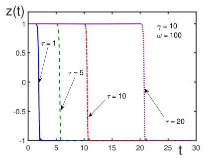
Figure 3: Spin polarization $z(t)$ of a nanocluster or nanomolecule as a function of time under dynamic resonance tuning, starting at different delay times: $\tau=1$ (solid line), $\tau=5$ (dashed line), $\tau=10$ (dash-dotted line), and $\tau=20$ (dotted line). Other parameters are fixed as $A=1$, $\omega_{E}=\omega_{1}=0.01$, $\omega=\omega_{0}=100$ and $\gamma=10$.

4 Assemblies of nanomolecules or nanoclusters

In the previous section, we have considered the realization of dynamic resonance tuning for single nanomolecules or nanoclusters, which allows for fast magnetization reversal at any required time. The natural question is whether it would be feasible to apply this effect for regulating spin dynamics of the assemblies of nanomolecules or nanoclusters.

The Hamiltonian of a system of nanomolecules or nanoclusters reads as

$$\hat{H}=-\mu_{S}\sum_{j}{\bf B}\cdot{\bf S}_{j}+\hat{H}_{A}+\hat{H}_{D}\;,$$ (21)

where $j=1,2,\ldots,N$ enumerates the clusters, the first is the Zeeman term and the second is the anisotropy term

$$\hat{H}_{A}=-\sum_{j}D(S_{j}^{z})^{2}\;.$$ (22)

The anisotropy parameter $E$ is usually much smaller than $D$, so it can be safely omitted.

In addition, there is the term responsible for the dipolar interactions of the constituents

$$\hat{H}_{D}=\frac{1}{2}\sum_{i\neq j}\;\sum_{\alpha\beta}D_{ij}^{\alpha\beta}S_{i}^{\alpha}S_{j}^{\beta}\;,$$ (23)

with the dipolar tensor

$$D_{ij}^{\alpha\beta}=\frac{\mu_{S}^{2}}{r_{ij}^{3}}\;\left(\delta_{\alpha\beta}-3n_{ij}^{\alpha}n_{ij}^{\beta}\right)\;,$$ (24)

in which

$$r_{ij}\equiv|\;{\bf r}_{ij}\;|\;,\qquad{\bf n}_{ij}\equiv\frac{{\bf r}_{ij}}{r_{ij}}\;,\qquad{\bf r}_{ij}\equiv{\bf r}_{i}-{\bf r}_{j}\;.$$

The sample is again inserted into a magnetic coil of an electric circuit. The total magnetic field is the sum

$${\bf B}=H{\bf e}_{x}+(B_{0}+\Delta B){\bf e}_{z}$$ (25)

of the feedback field $H$, a constant external magnetic field $B_{0}$, and a regulated field $\Delta B$.

The feedback field satisfies equation (4), but with the right-hand side, describing the electromotive force, containing the average magnetization

$$m_{x}=\frac{\mu_{S}}{V}\sum_{j}\langle\;S_{j}^{x}\;\rangle\;.$$ (26)

The coil axis is again aligned with the $x$ axis.

In what follows, it is convenient to employ the ladder spin operators $S_{j}^{\pm}=S_{j}^{x}\pm iS_{j}^{y}$. We introduce the average transverse spin component

$$u=\frac{1}{SN}\sum_{j}\langle\;S_{j}^{-}\;\rangle\;,$$ (27)

the coherence intensity

$$w=\frac{1}{SN(N-1)}\sum_{i\neq j}\langle\;S_{i}^{+}S_{j}^{-}\;\rangle\;,$$ (28)

and the longitudinal spin polarization

$$s=\frac{1}{SN}\sum_{j}\langle\;S_{j}^{z}\;\rangle\;.$$ (29)

Local spin fluctuations, caused by dipolar interactions, are characterized by the expressions

$$\xi_{S}=\frac{1}{\hbar}\sum_{j}\langle\;a_{ij}S_{j}^{z}+c_{ij}S_{j}^{+}+c_{ij}^{*}S_{j}^{-}\;\rangle\;,$$

$$\varphi_{S}=\frac{1}{\hbar}\sum_{j}\left\langle\;\frac{a_{ij}}{2}\;S_{j}^{-}-2b_{ij}S_{j}^{+}-2c_{ij}S_{j}^{z}\;\right\rangle\;,$$ (30)

in which

$$a_{ij}\equiv D_{ij}^{zz}\;,\qquad b_{ij}\equiv\frac{1}{4}\;\left(D_{ij}^{xx}-D_{ij}^{yy}-2iD_{ij}^{xy}\right)\;,\qquad c_{ij}\equiv\frac{1}{2}\;\left(D_{ij}^{xz}-iD_{ij}^{yz}\right)\;.$$

These expressions are responsible for dipolar spin waves initiating spin motion at the beginning of the process [32].

The decoupling of pair spin correlators is accomplished in the corrected mean-field approximation

$$\langle\;S_{i}^{\alpha}S_{j}^{\beta}\;\rangle=\langle\;S_{i}^{\alpha}\;\rangle\langle\;S_{j}^{\alpha}\;\rangle\qquad(i\neq j)\;,$$

$$\langle\;S_{j}^{\alpha}S_{j}^{\beta}+S_{j}^{\beta}S_{j}^{\alpha}\;\rangle=\left(2-\;\frac{1}{S}\right)\;\langle\;S_{j}^{\alpha}\;\rangle\langle\;S_{j}^{\beta}\;\rangle$$ (31)

accurately taking into account the terms describing magnetic anisotropy [31]. Writing down the spin equations of motion and averaging them, we come to the system of equations

$$\frac{du}{dt}=-i(\omega_{S}+\xi_{S}-i\gamma_{2})\;u+fs\;,\qquad\frac{dw}{dt}=-2\gamma_{2}w+(u^{*}f+f^{*}u)\;s\;,$$

$$\frac{ds}{dt}=-\;\frac{1}{2}\;(u^{*}f+f^{*}u)\;,$$ (32)

with the transverse attenuation

$$\gamma_{2}=\frac{1}{\hbar}\;\rho\;\mu_{S}^{2}S\;,$$ (33)

where $\rho=N/V$ is spin density, and the effective force

$$f=-i\left(\frac{\mu_{S}H}{\hbar}+\varphi_{S}\right)\;.$$ (34)

The effective Zeeman frequency here is

$$\omega_{S}=\omega_{0}(1+b-As)\;,$$ (35)

where the dimensionless regulated field $b$ is defined in Eq. (11).

The feedback-field equation (4) can be represented in the integral form

$$H=-4\pi\eta_{res}\int_{0}^{t}G(t-t^{\prime})\;\dot{m}_{x}(t^{\prime})\;dt^{\prime}\;,$$ (36)

with the transfer function

$$G(t)=\left[\;\cos(\omega^{\prime}t)\;-\;\frac{\gamma}{\omega^{\prime}}\;\sin(\omega^{\prime}t)\;\right]\;e^{-\gamma t}\;,$$

where the frequency is

$$\omega^{\prime}\equiv\sqrt{\omega^{2}+\gamma^{2}}\;.$$

The electromotive force is expressed through

$$\dot{m}_{x}=\frac{1}{2}\;\rho\;\mu_{S}S\;(u^{*}+u)\;.$$ (37)

The coupling rate is

$$\gamma_{0}=\pi\eta_{res}\gamma_{2}\;.$$ (38)

As usual, the attenuations are small as compared to the related frequencies:

$$\frac{\gamma_{0}}{\omega}\ll 1\;,\qquad\frac{\gamma}{\omega}\ll 1\;,\qquad\frac{\gamma_{2}}{\omega_{0}}\ll 1\;.$$ (39)

The solution to the feedback field, following from Eq. (36), to the first order in $\gamma_{0}$ reads as

$$\mu_{S}H=i\hbar\;(uX-X^{*}u^{*})\;,$$ (40)

with the coupling function

$$X=\gamma_{0}\;\omega_{S}\;\frac{1-\exp(-i\Delta_{S}t-\gamma t)}{\gamma+i\Delta_{S}\;{\rm sign}\;\omega_{S}}$$ (41)

and the dynamic detuning

$$\Delta_{S}=\omega-|\;\omega_{S}\;|\;.$$ (42)

The presence of the small parameters (39) makes it straightforward to resort to the averaging techniques [37, 38], with considering the dipolar spin fluctuations, characterized by expressions (30), as small random variables [39, 40]. Due to the small parameters (39), the function $u=u(t)$ in Eqs. (32) has to be treated as a fast variable, while the functions $w=w(t)$ and $s=s(t)$, as slow variables. With the slow variables playing the role of adiabatic invariants, we solve the equation for the fast variable, yielding

$$u=u_{0}\exp\left\{-i\Omega t-i\int_{0}^{t}\xi_{S}(t^{\prime})\;dt^{\prime}\right\}\;-$$

$$-\;is\int_{0}^{t}\varphi_{S}(t^{\prime})\;\exp\left\{-i\Omega(t-t^{\prime})-i\int_{t^{\prime}}^{t}\xi_{S}(t^{\prime\prime})\;dt^{\prime\prime}\right\}\;dt^{\prime}\;,$$ (43)

where

$$\Omega=\omega_{S}-i(\gamma_{2}-Xs)\;.$$

Then, substituting the solutions for the feedback field (41) and for the fast variable (43) into the equations for the slow variables $w$ and $s$, we average the latter over time and random spin fluctuations [41]. As a result, we obtain the guiding-center equations

$$\frac{dw}{dt}=2\gamma_{2}w(\alpha s-1)+2\gamma_{3}s^{2}\;,\qquad\frac{ds}{dt}=-\gamma_{2}\alpha w-\gamma_{3}s\;,$$ (44)

in which we define the coupling function

$$\alpha\equiv\frac{{\rm Re}X}{\gamma_{2}}=\frac{\gamma_{0}\gamma\omega_{S}}{\gamma_{2}(\gamma^{2}+\Delta_{S}^{2})}\left\{1-[\;\cos(\Delta_{S}t)-\delta_{S}\sin(\Delta_{S}t)\;]\;e^{-\gamma t}\right\}\;,$$ (45)

the relative detuning

$$\delta_{S}\equiv\frac{\Delta_{S}}{\gamma}\;{\rm sign}\;\omega_{S}\;,$$ (46)

and the spin-wave attenuation

$$\gamma_{3}=\frac{\gamma_{2}^{2}}{\sqrt{\omega_{S}^{2}+\gamma_{2}^{2}}}\;.$$ (47)

As initial conditions, we take $w(0)=0$, which implies the absence of triggering fields, so that the process is self-organized, and we assume the initial average spin polarization up, so that $s(0)=1$.

5 Dynamic resonance tuning for spin assemblies

Suppose we wish to keep the average spin polarization up until the time $\tau$ and then we need to quickly reverse the average spin. For this purpose, we set $\omega_{0}=\omega$ and arrange the regulated magnetic field according to the law

$$b(t)=\left\{\begin{array}[]{ll}0\;,{}&~{}t<\tau\\ As_{reg}\;,{}&~{}t\geq\tau\;,\end{array}\right.$$ (50)

with the parameter

$$A\equiv\frac{\omega_{D}}{\omega_{0}}$$ (51)

and with $s_{reg}$ satisfying the equations

$$\frac{ds_{reg}}{dt}=-\gamma_{2}\alpha_{reg}w_{reg}-\gamma_{reg}s_{reg}\;,$$

$$\frac{dw_{reg}}{dt}=2\gamma_{2}w_{reg}(\alpha_{reg}s_{reg}-1)+2\gamma_{reg}s_{reg}^{2}\;.$$ (52)

In the latter, the effective coupling function is

$$\alpha_{reg}=g\left(1-e^{-\gamma t}\right)\;,$$ (53)

with the coupling parameter

$$g\equiv\frac{\gamma_{0}\omega_{0}}{\gamma\gamma_{2}}$$ (54)

and the attenuation

$$\gamma_{reg}\equiv\frac{\gamma_{2}^{2}}{\sqrt{\omega^{2}+\gamma_{2}^{2}}}\;.$$ (55)

The initial conditions at time $\tau$ are $w_{reg}(\tau)=w(\tau)$ and $s_{reg}(\tau)=s(\tau)$. At time $\tau$, there is the resonance $\omega_{0}=\omega$, and in the following times the regulated field (50) varies so that the system is dynamically captured into resonance [42].

If there is need for repeating the overall process again, this can be done by either inversing the direction of the external field $B_{0}$ or by rotating the sample as has been described for organizing a Morse-code alphabet functioning of spin pulses for samples having no magnetic anisotropy [43].

Figures 4 and 5 demonstrate the effect of dynamic resonance tuning for the assemblies of magnetic nanomolecules or nanoclusters. The average spin of the system can be kept for a long time by a strong magnetic anisotropy. The spin is better frozen for larger anisotropies and larger Zeeman frequencies. Employing dynamic resonance tuning makes it possible to realize an ultrafast spin reversal at any required time.

     

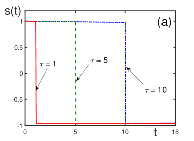
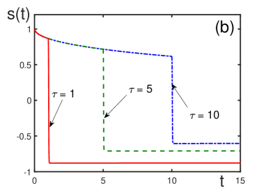
Figure 4: Average spin polarization $s(t)$ of an assembly of magnetic nanomolecules or nanoclusters for $\omega=\omega_{0}=100$ and $\gamma=10$ as a function of time under dynamic resonance tuning starting at different delay times: $\tau=1$ (solid line), $\tau=5$ (dashed line), and $\tau=10$ (dash-dotted line). The anisotropy parameters are: (a) $A=5$; (b) $A=1$.

     

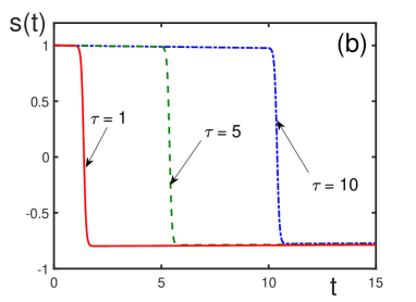
Figure 5: Average spin polarization $s(t)$ of an assembly of magnetic nanomolecules or nanoclusters for the anisotropy parameter $A=5$ and $\gamma=10$. The dynamic resonance tuning starts at different delay times: $\tau=1$ (solid line), $\tau=5$ (dashed line), and $\tau=10$ (dash-dotted line). Resonance frequencies are: (a) $\omega=\omega_{0}=1000$; (b) $\omega=\omega_{0}=100$.

6 Discussion and conclusion

We have suggested a method allowing, by using magnetic nanosystems, such as magnetic nanomolecules and nanoclusters, to combine two features that are crucially important for the functioning of memory devices, the possibility of keeping for long times a frozen magnetization that can be reversed at a required time. The method is based on the following technical stratagems. First, it is straightforward to use the property of magnetic nanomolecules and nanoclusters to keep, below the blocking temperature, the direction of magnetization frozen in a metastable state. Second, the sample is inserted into a magnetic coil of an electric circuit creating a magnetic feedback field. Third, at a required time, a varying magnetic field is imposed, varying in such a way that to dynamically support a resonance between the electric circuit and the varying Zeeman frequency of the sample. Recall that the effective Zeeman frequency changes in time because of the interaction between the moving sample spin and the magnetic anisotropy field. Due to this dynamic resonance, there develops a strong coupling between the sample and the electric circuit, that is between the sample spin and the resonator feedback field, which realizes an ultrafast spin reversal. This procedure can be implemented for single nanomolecules or nanoclusters as well as for their assemblies. The process is illustrated by numerically solving the spin equations of motion.

In order to grasp the typical values of the empirical parameters, let us adduce several examples. Thus the typical parameters of Co, Fe, and Ni nanoclusters are as follows. A single cluster, of volume around $V\sim 10^{-20}$ cm³, can contain about $N\sim 10^{3}-10^{4}$ atoms, so that the total cluster spin can be $S\sim 10^{3}-10^{4}$. The blocking temperature is $T_{B}\sim(10-100)$ K. With the magnetic field $B_{0}\sim 1$ T, the Zeeman frequency is $\omega_{0}\sim 10^{11}$ s^-1. The feedback rate is of order $\gamma_{0}\sim(10^{10}-10^{11})$ s^-1. The typical anisotropy parameters are $D/\hbar\sim 10^{7}$ s^-1 and $E/\hbar\sim 10^{6}$ s^-1 or $\omega_{D}\sim 10^{10}-10^{11}$ s^-1 and $\omega_{E}\sim 10^{9}-10^{10}$ s^-1. Hence the dimensionless anisotropy parameter can be $A\sim 0.1-1$.

The magnetic nanomolecule, named Fe₈, possesses the spin $S=10$, blocking temperature $T_{B}\approx 1$ K, the molecule volume $V\sim 10^{-20}$ cm³, the anisotropy parameters $D/k_{B}=0.27.5$ K and $E/k_{B}=0.046$ K, or $D/\hbar\sim 4\times 10^{10}$ s^-1 and $E/\hbar\sim 10^{10}$ s^-1. Thus, the anisotropy frequencies are $\omega_{D}\sim 4\times 10^{11}$ s^-1 and $\omega_{E}\sim 10^{11}$ s^-1. Then the dimensionless anisotropy parameter is $A\sim 1-4$.

The magnetic nanomolecule Mn₁₂ also has the spin $S=10$ and the blocking temperature $3.3$ K. The spin polarization can be kept frozen for very long times depending on temperature and defined by the Arrhenius law. For example, at $T=3$ K, the spin is frozen for one hour and at $2$ K, for $2$ months. The molecule radius is around $10^{-7}$ cm and the volume, $V\sim 10^{-20}$ cm³. The Zeeman frequency, for $B_{0}=1$ T, is $\omega_{0}\sim 10^{11}$ s^-1. The feedback rate is $\gamma_{0}\sim 10^{8}$ s^-1. The anisotropy parameter $D/k_{B}\approx 0.6$ K and $D/\hbar\sim 10^{11}$ s^-1, while the value of $E$ is negligible. The anisotropy frequency is $\omega_{D}\sim 10^{12}$ s^-1. Therefore the dimensionless anisotropy parameter is $A\sim 10$.

These values of the parameters have been kept in mind in our numerical calculations. The reversal time is $t_{rev}\approx\gamma/(\gamma_{0}\omega_{0}s_{0})$. For $\gamma\approx\gamma_{0}$ and $\omega\sim 10^{11}$ s^-1, the reversal time is of order $t_{rev}\sim 10^{-11}$ s.

References

- [1] Barbara B, Thomas L, Lionti F, Chiorescu I and Sulpice A 1999 J. Magn. Magn. Mater. 200 167
- [2] Caneschi A, Gatteschi D, Sangregorio C, Sessoli R, Sorace L, Cornia A, Novak M A, Paulsen C W and Wernsdorfer W 1999 J. Magn. Magn. Mater. 200, 182
- [3] Yukalov V I 2002 Laser Phys. 12, 1089
- [4] Yukalov V I and Yukalova E P 2004 Phys. Part. Nucl. 35 348
- [5] Yukalov V I and Yukalova E P 2005 Eur. Phys. Lett. 70 306
- [6] Yukalov V I and Yukalova E P 2005 Laser Phys. Lett. 2 302
- [7] Friedman J R and Sarachik M P 2010 Annu. Rev. Condens. Matter Phys. 1 109
- [8] Miller J S 2014 Mater. Today 17 224
- [9] Craig G A and Murrie M 2015 Chem. Soc. Rev. 44 2135
- [10] Liddle S T and van Slageren J 2015 Chem. Soc. Rev. 44 6655
- [11] Rana B, Mondal A K, Bandyopadhyay A and Barman A 2021 Nanotechnology 33 062007
- [12] Kodama R H 1999 J. Magn. Magn. Mater. 200 359
- [13] Hadjipanays G C 1999 J. Magn. Magn. Mater. 200 373
- [14] Wernsdorfer W 2001 Adv. Chem. Phys. 118 99
- [15] Yukalov V I and Yukalova E P 2011 Laser Phys. Lett. 8 804
- [16] Kudr J, Haddad Y, Richtera L, Heger Z, Cernak M, Adam V and Zitka O 2017 Nanomaterials 7 243
- [17] Griesmaier A 2007 J. Phys. B 40 R91
- [18] Baranov M A 2008 Phys. Rep. 464 71
- [19] Baranov M A, Dalmonte M, Pupillo G and Zoller P 2012 Chem. Rev. 112 5012
- [20] Stamper-Kurn D M and Ueda M 2013 Rev. Mod. Phys. 85 1191
- [21] Gadway B and Yan B 2016 J. Phys. B 49 152002
- [22] Yukalov V I and Yukalova E P 2018 Eur. Phys. J. D 72 190
- [23] Yukalov V I 2018 Laser Phys. 28 053001
- [24] Yukalov V I, Henner V K and Belozerova T S 2016 Laser Phys. Lett. 13 016001
- [25] Yukalov V I, Henner, V K, Belozerova T S and Yukalova E P 2016 J. Supercond. Nov. Magn. 29 721
- [26] Birman J L, Nazmitdinov R G and Yukalov V I 2013 Phys. Rep. 526 1
- [27] Schwartz D A, Norberg N S, Nguyen Q P, Parker J M and Gamelin D R 2003 J. Am. Chem. Soc. 125 13205
- [28] Koole R, Mulder W J M, van Schooneveld M M, Strijkers G J, Meijerink A and Nicolay K 2009 Wiley Interdiscip. Rev. Nanomed. Nanobiotechnol. 1 475
- [29] Mahajan K D, Fan Q, Dorcena J, Ruan G and Winter J O 2013 Biotechnol. J. 8 1424
- [30] Tufani A, Qureshi A and Niazi J H 2021 Mater. Sci. Eng. C 118 111545
- [31] Yukalov V I 1996 Phys. Rev. B 53 9232
- [32] Yukalov V I 2005 Phys. Rev. B 71 184432
- [33] Yukalov V I, Henner V K and Kharebov P V 2008 Phys. Rev. B 77 134427
- [34] Yukalov V I and Yukalova E P 2012 J. Appl. Phys. 111 023911
- [35] Kharebov P V, Henner V K and Yukalov V I 2013 J. Appl. Phys. 113 043902
- [36] Yukalov V I and Yukalova E P 2022 Laser Phys. Lett. 19 046001
- [37] Bogolubov N N and Mitropolsky Y A 1961 Asymptotic Methods in the Theory of Nonlnear Equations (New York: Gordon and Breach)
- [38] Freidlin M I and Wentzell A D 1984 Random Perturbations of Dynamical Systems (New York: Springer)
- [39] Gardiner C W 1983 Handbook of Stochastic Methods (Berlin: Springer)
- [40] Yukalov V I and Yukalova E P 2000 Phys. Part. Nucl. 31 561
- [41] Yukalov V I and Yukalova E P 2018 Phys. Rev. B 98 144438
- [42] Lochak P and Meunier C 1988 Multiphase Averaging for Classical Systems (New York: Springer)
- [43] Yukalov V I and Yukalova E P 2002 Phys. Rev. Lett. 88 257601