Notes on a 1-dimensional electrostatic plasma model

Abstract

A starting point for deriving the Vlasov equation is the BBGKY hierarchy that describes the dynamics of coupled marginal distribution functions.   With a large value of the plasma parameter one can justify eliminating 2-point correlations in terms of the 1-point function in order to derive the Vlasov Landau Lenard Balescu (VLLB) theory. Because of the high dimensionality of the problem, numerically testing the assumptions of the VLLB theory is prohibitive.   In these notes we propose a physically reasonable interaction model that lowers the dimensionality of the problem and may bring such computations within reach. We introduce a 1-dimensional (1-D) electrostatic plasma model formulated in terms of the interaction of parallelly-aligned charged disks. This model combines 1-dimensional features at short distances and 3-dimensional features at large distances.

1 Introduction

The construction of a charged-disks electrostatic model is motivated by the aim [1] to verify numerically the validity of the procedure which is adopted, see e.g. Ref.[2], in order to solve the BBGKY hierarchy [3] in a weakly coupled plasma when deriving the kinetic plasma equation, i.e. the Vlasov equation. Such a verification might be based on the numerical integration of the time evolution of the two-point particle distribution function as obtained from a proper Hamiltonian truncation of the the BBGKY hierarchy at the level of the three-point distribution function [4]. In 3-D space the equation for the time evolution of this two-point distribution function would be 13-dimensional (one time dimension plus the 12-dimensional two-particle phase space). In 1-D space the equation for the two-point (actually two foil) distribution would be 5-dimensional (time plus 4-dimensional two-foil phase space). However in 1-D the electric field generated by a charge foil does not decay with distance so that the two-foil interaction energy diverges at infinity. This makes it impossible to define a finite correlation length. A possible compromise is to consider the interaction of aligned, uniformly charged disks, a sort of a single-row abacus made of thin disk-shaped beads, where we can introduce a characteristic length $b$, the radius of the disk, which we may identify with the Debye radius $\lambda_{d}$ (same for the electrons and ions). In this case the electrostatic interaction energy between two charged disks is finite both at zero and at infinite distance $\xi$ from the source and its absolute value is a decreasing function of $\xi$.

The present notes are dedicated to the derivation of the main properties of such a disk-plasma in order to clarify where and how the dynamics of such a model system can mimic the dynamics of a real plasma, at least as long as the longitudinal electric field limit is concerned. In analogy with a real particle plasma, in the derivation which follows we will introduce concepts such as positive and negative charged disk densities, collective electric field shielding, disk waves etc., but we will not use a Poisson type equation with the charge disk density as the source. It will be enough to refer to the expression of the interaction energy between the disks derived in Ref.[5] that in the present model will play the role of the inter-particle Coulomb energy in a real 3-D plasma.

2 Disk Model

The “disk model” describes a globally neutral system consisting of a large number (as calculated inside intervals with length of the order of the disk radius $b$) of aligned, infinitely thin disks with equal radius, as sketched in Fig.1, equal or opposite electric charge and different masses (ion-disks, electron-disks) that are free to move along the $x$ axis (the planes of the disks are orthogonal to the $x$ axis) and to pass through each other.

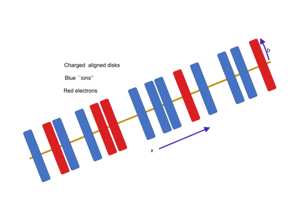
Figure 1: Schematic view, not in scale, of the disk configuration with the different colours representing different charges.

In the following, for the sake of simplicity, the ion-disks are taken to be immobile. We denote the mass of an electron disk by $M_{e}$ and its charge by $Q_{e}=-Q_{i}$ with $Q_{i}$ the charge of an ion disk.

2.1 Discrete disks: interaction energy

The interaction energy ${\cal W}(x_{1},x_{2})$ between two uniformly charged infinitely thin disks of radius $b$ located at $x_{1}$ and $x_{2}$ respectively can be written in c.g.s. units as [5].

$${\cal W}(x_{1},x_{2})=4\frac{Q_{1}\,Q_{2}}{b}V(\xi)=Q_{1}\varphi_{2}=Q_{2}\varphi_{1},$$ (1)

where

$$V(\xi)=-\frac{\xi}{2}\left\{1-\frac{1}{3\pi}\left[(4-\xi^{2})E(-4/\xi^{2})+(4+\xi^{2})K(-4/\xi^{2})\right]\right\}.$$ (2)

and $\varphi_{1}$, $\varphi_{2}$ are the potentials generated by the disks $1$ and $2$ respectively. Here $\xi(x_{1},x_{2})=|x_{1}-x_{2}|/b$, $Q_{1}=\pi b^{2}\sigma_{1}$ and $Q_{2}=\pi b^{2}\sigma_{2}$ are the (fixed) charges of the two disks, $\sigma_{1,2}$ are their surface density and $E(-4/\xi^{2})$ and $K(-4/\xi^{2})$ are elliptic integrals [6]. The “disks-electrostatics” is illustrated in more detail in Appendix A. A plot of $V(\xi)$ is given in Fig.2 .

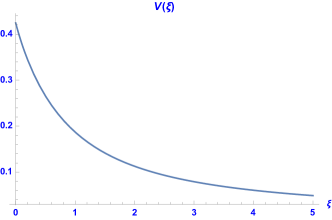
Figure 2: Plot of the potential $V(\xi)$ versus $\xi$.  Note the $1/(4\xi)$-behavior for large $\xi$ and the finite value $4/(3\pi)$ at $\xi=0$.

The corresponding electric force ${\cal F}_{Q_{2}}$ acting on the disk 1 due to the disk 2 is given by

$${\cal F}_{Q_{2}}(x_{1})=-{\cal F}_{Q_{1}}(x_{2})=-(4Q_{1}Q_{2}/b^{2})\,V^{\prime}(\xi)\,{\rm sign}\,(x_{1}-x_{2}),\qquad{\rm where}\quad$$ (3)

$$V^{\prime}(\xi)=\frac{dV(\xi)}{d\xi}=\left[\frac{1}{2}+\frac{1}{2\pi}\left[\xi^{2}E(-4/\xi^{2})-(4+\xi^{2})K(-4/\xi^{2})\right]\right].$$

A plot of $-V^{\prime}(\xi)$ is given in Fig.3

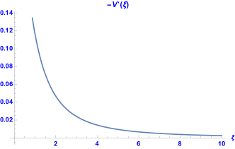
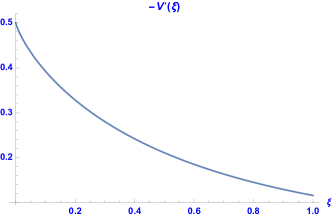
Figure 3: Plot of $-V^{\prime}(\xi)$ versus $\xi$.  Note the $1/(4\xi^{2})$ behavior for large $\xi$ (left frame) and the value $-V^{\prime}(0)=1/2$ (right frame).

3 Continuous limit

Define an electron-disk density $n_{e}(x,t)$ (number of disks per unit length) and an ion-disk density $n_{i}(x,t)=n_{i}$ (for simplicity stationary and homogeneous). This defines a disk-charge density (charge per unit length)

$$\rho(x)=Q(n_{i}-n_{e}(x,t)),$$ (4)

with $Q=Q_{i}=-Q_{e}$.

Define the electron-disk velocity $u_{e}(x,t)$ that satisfies the continuity equation

$$\partial_{t}n_{e}(x,t)+\partial_{x}[n_{e}(x,t)\,u_{e}(x,t)]=0.$$ (5)

Assuming that $n_{i}-n_{e}(x,t)$ vanishes (sufficiently fast) at $\pm\infty$, the electrostatic potential created by a disk-charge density can be written in convolution integral form as

$$\varphi(x)=(4/b)\int_{-\infty}^{+\infty}dx^{\prime}\rho(x^{\prime})V(|x-x^{\prime}|/b),$$ (6)

which returns for $\rho(x^{\prime})=Q\delta(x^{\prime}-x_{1})$ the expression for the potential of a disk given in Eq.(1).

The corresponding electric force acting on a disk of charge $Q_{j}$   ($j=i,e$) can be written as

$${\cal F}_{j}(x)=-(4Q_{j}/b)\frac{d}{dx}\int_{-\infty}^{+\infty}dx^{\prime}\,\rho(x^{\prime})V(|x-x^{\prime}|/b),$$ (7)

which returns Eq.(3) for $\rho(x^{\prime})=Q_{1}\delta(x^{\prime}-x_{1})$. To close the system we may supplement the continuity equation (5) with the momentum equation of a “cold” disk plasma

$$M_{e}n_{e}\left(\partial_{t}+u_{e}\partial_{x}\right)u_{e}=n_{e}{\cal F}_{e}.$$ (8)

In the rest of this section we find it convenient to use dimensionless dynamical quantities based on a characteristic time (the inverse of the disk plasma frequency, see Eq.(33))

$$\omega_{Dpe}^{-1}=\left[{4Q^{2}n_{o}}/{M_{e}b^{2}}\right]^{-1/2},$$ (9)

where $n_{0}$ is the (uniform) background density, and on the length $d$ (note that the disk electrostatic, contrary to standard electrostatic, has a characteristic spatial scale).    Specifically we set

$$\tau=t\,\omega_{Dpe},\quad{\rm and}\quad X=x/b,$$ (10)

in agreement with the definition of the variable $\xi$. Then we define

$$N_{e,i}(X,\tau)=b\,n_{e,i}(x,t),\quad\varrho(X,\tau)=b\,\rho(x,t)=Q(N_{i}-N_{e}),\$$ (11)

$$u_{e}(x,t)=v_{D}\,U_{e}(X,\tau)\quad{\rm where}\quad v_{D}=b\,\omega_{Dpe}=[{4Q^{2}n_{o}}/{M_{e}}]^{1/2},\quad\Phi(X)=b\,\varphi(x)/4,$$

$$\quad F_{e}=b^{2}/(4Q^{2}N_{0}){\cal F}_{e}(x)=\frac{1}{N_{0}Q}\frac{d}{dX}\int_{-\infty}^{+\infty}dX^{\prime}\,\,\varrho(X^{\prime})V(|X-X^{\prime}|/b),$$

where $\varrho(X^{\prime})/(N_{0}Q)=(N_{i}-N_{e})/N_{0}$ is dimensionless. Note that in a particle plasma there is no velocity directly corresponding to $v_{D}$. Then Eqs.(5,8) read

$$\partial_{\tau}N_{e}(X,\tau),+\partial_{X}[N_{e}(X,\tau)\,U_{e}(X,\tau)]=0,$$

$$N_{e}\left(\partial_{\tau}+U_{e}\partial_{X}\right)U_{e}=F_{e},$$ (12)

with

$$F_{e}=\frac{d}{dX}\ \int_{-\infty}^{+\infty}dX^{\prime}\,\frac{N_{i}-N_{e}(X^{\prime})}{N_{0}}\,V(|X-X^{\prime}|).$$ (13)

3.0.1 Laplace transform representation

Start from Eq.(6) with the potential $\varphi(x)=(4/b)\int_{-\infty}^{+\infty}dx^{\prime}\rho(x^{\prime})V(|x-x^{\prime}|/b)$ and write the integral in dimensionless form

$$\int_{-\infty}^{+\infty}dx^{\prime}\rho(x^{\prime})V(|x-x^{\prime}|)=\int_{0}^{+\infty}ds[J_{1}(s)/s]^{2}\,\int_{-\infty}^{+\infty}dx^{\prime}\rho(x^{\prime})\exp{(-s(|x-x^{\prime}|)},$$ (14)

where $J_{1}$ is a Bessel function and we used Eq.(46). The double-sided Laplace transform in $dx^{\prime}$ can be written as

$$\int_{-\infty}^{+\infty}dx^{\prime}\rho(x^{\prime})\exp{(-s(|x-x^{\prime}|)}=\int_{x}^{+\infty}dx^{\prime}\rho(x^{\prime})\exp{[s(x-x^{\prime})]}+\int^{x}_{-\infty}dx^{\prime}\rho(x^{\prime})\exp{[s(x^{\prime}-x)]}$$

$$=\int_{0}^{+\infty}dy\,\rho(x+y)\exp{[-sy]}+\int_{-\infty}^{0}d\eta\,\rho(x+\eta)\exp{[s\eta]}$$

$$=\int_{0}^{+\infty}dy\,[\rho(x+y)+\rho(x-y)]\exp{[-sy]}.$$ (15)

Thus we obtain

$$\int_{-\infty}^{+\infty}dx^{\prime}\rho(x^{\prime})V(|x-x^{\prime}|)=\int_{0}^{+\infty}ds[J_{1}(s)/s]^{2}\,\int_{0}^{+\infty}dy\,[\rho(x+y)+\rho(x-y)]\exp{[-sy]}.$$ (16)

Computing the integral over $s$ first would bring us essentially to the initial Eq.(6). On the contrary it is convenient to use the fact that Eq.(16) contains a special combination of Poisson transforms of the density $\rho(x)$ and expand $\rho(x)$ on a basis with elements that transform in a simple way under Poisson transform.

Thus we write the Fourier series (finite domain, periodic boundary conditions)

$$\rho(x)=\Sigma_{n=0}^{\infty}[C_{n}\cos{(nx)}+S_{n}\sin{(nx)}],$$ (17)

use the relationships

$$\int_{0}^{+\infty}dy\,\cos{(ay+b)}\exp{[-sy]}=\frac{s\cos{(b)}-a\sin{(b)}}{s^{2}+a^{2}}$$

$$\int_{0}^{+\infty}dy\,\sin{(ay+b)}\exp{[-sy]}=\frac{s\sin{(b)}+a\cos{(b)}}{s^{2}+a^{2}}.$$ (18)

and obtain

$$\int_{0}^{+\infty}dy\,[\rho(x+y)+\rho(x-y)]\exp{[-sy]}=$$ (19)

$$\int_{0}^{+\infty}dy\exp{[-sy]}\,\ \Sigma_{n=0}^{\infty}\{C_{n}[\cos{[n(y+x)]+\cos[n(y-x)}+S_{n}[\sin{[n(y+x)]}-\sin{[n(y-x)]}\}$$

$$=\Sigma_{n=0}^{\infty}\,\frac{2s}{s^{2}+n^{2}}[C_{n}\cos{(nx)}+S_{n}\sin{(nx)}].$$ (20)

Thus finally we have

$$\int_{-\infty}^{+\infty}dx^{\prime}\rho(x^{\prime})V(|x-x^{\prime}|)=\Sigma_{n=0}^{\infty}\,\,[C_{n}\cos{(nx)}+S_{n}\sin{(nx)}]\,\int_{0}^{+\infty}ds\frac{2J^{2}_{1}(s)}{s(s^{2}+n^{2})},$$ (21)

where the last integral is a known function (see Eq.(47.)

3.0.2 Fourier space

Assuming the required boundary conditions at infinity, we write

$${\hat{\rho}}(k)=\frac{1}{(2\pi)^{1/2}}\int_{-\infty}^{+\infty}dx\,\rho(x)\,\exp{(-ikx)},\quad{\hat{\cal F}}_{j}(k)=\frac{1}{(2\pi)^{1/2}}\int_{-\infty}^{+\infty}dx\,{\cal F}_{j}(x)\exp{(-ikx)}$$ (22)

and obtain from Eq.(7), which has the form of a convolution integral,

$${\hat{\cal F}}_{j}(k)=-\frac{Q_{j}}{4b}\frac{1}{(2\pi)^{1/2}}\int_{-\infty}^{+\infty}dx\,\exp{(-ikx)}\frac{d}{dx}\int_{-\infty}^{+\infty}dx^{\prime}\,\rho(x^{\prime})V(|x-x^{\prime}|/b),$$ (23)

$$=-\frac{4Q_{j}}{b}\frac{ik}{(2\pi)^{1/2}}\int_{-\infty}^{+\infty}dx\,\exp{(-ikx)}\int_{-\infty}^{+\infty}dx^{\prime}\,\rho(x^{\prime})V(|x-x^{\prime}|/b),=-4ikQ_{j}{\hat{\rho}}(k){\hat{V}}(kb),$$

where ${\hat{V}}(kb$) is defined (without including the factor $1/(2\pi)^{1/2}$) by

$${\hat{V}}(kb)=\int_{-\infty}^{+\infty}\frac{dx}{b}\,\,V(|x|/b)\exp{-[i(kb)\,(x/b)]}]=2\int_{0}^{+\infty}{dx}/{b}\,\,V(|x|/b)\cos{[(kb)\,(x/b)}]$$ (24)

and is explicitly calculated in Appendix A.

, .

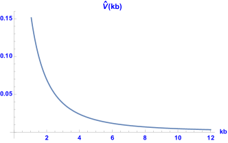
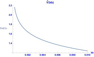
Figure 4: Behavior of ${\hat{V}}(kb)$ for large (left frame) a for small values (right frame) displaying the logarithmic contribution, see Eq.(A).

3.1 Screening at thermodynamic equilibrium

In order to determine the screening of a test disk of charge $Q_{t}$ at $x=0$ produced by the spatial rearranging of the other disks we consider an electron-disk Boltzmann equilibrium expressed in terms of the screened potential $\varphi_{s}$

$$n_{e}(x)=n_{e}(o)\exp{[(Q\varphi_{s})/T_{e}]}\sim n_{e}(o)[1+Q\varphi_{s}/T_{e}].$$ (25)

Note that in this disk model, contrary to a Coulomb plasma, the approximation $Q\varphi_{s}/T_{e}\ll 1$ remains valid even at close distance. Setting $n_{i}=n_{e}(o)=n_{o}$ we can write the charge density of the test disk plus the screening density obtained from Eq.(25)

$$\rho(x)=Q_{t}\delta(x)-Q^{2}n_{o}\varphi_{s}/T_{e},$$ (26)

which inserted into Eq.(6) gives the integral equation

$$\varphi_{s}(x)=Q_{t}(4/b)V(|x|/b)-4(Q^{2}n_{o}/T_{e})\int_{-\infty}^{+\infty}\frac{dx^{\prime}}{b}\varphi_{s}(x^{\prime})V(|x-x^{\prime}|/b).$$ (27)

Since the integral term in Eq.(27) is a convolution product, Eq.(27) can be solved by performing a Fourier transform with respect to $x$ (see Appendix A for analytical details of the functions involved). Note that the factor in front of the integral is dimensionless and can be interpreted as $\sim b^{2}/\lambda_{d}^{2}\sim 1$ if we recall that $n_{o}$ is the number of disks per unit length and that the disk radius is $b\sim\lambda_{d}$.

The Fourier transform of Eq.(27) reads

$${\hat{\varphi}}_{s}(kb)=Q_{t}(4/b){\hat{V}}(kb)-4(Q^{2}n_{o}/T_{e}){\hat{\varphi}}_{s}(kb)\,{\hat{V}}(kb),$$ (28)

where

$${\hat{\varphi}}_{s}(kb)=\frac{1}{(2\pi)^{1/2}}\int_{-\infty}^{+\infty}dx/b\,\,\varphi_{s}(x)\,\exp{-i[(kb)\,(x/b)]},$$ (29)

$${\hat{V}}(kb)=\int_{-\infty}^{+\infty}{dx}/{b}\,\,V(|x|/b)\exp{-[i(kb)\,(x/b)]}]=2\int_{0}^{+\infty}{dx}/{b}\,\,V(|x|/b)\cos{[(kb)\,(x/b)}].$$

The definition of ${\hat{V}}(kb)$ corresponds to $(2\pi)^{1/2}$ times the Fourier transform of $V(X)$. From Eq.(28) we obtain

$$[1+4(Q^{2}n_{o}/T_{e})\,{\hat{V}}(kb)]{\hat{\varphi}}_{s}(kb)=Q_{t}(4/b){\hat{V}}(kb),\quad{\rm i.e.}$$

$$\varphi_{s}(x)=\frac{1}{(2\pi)^{1/2}}\int_{-\infty}^{+\infty}{d(kb})\,\frac{Q_{t}(4/b){\hat{V}}(kb)\exp{[i(kb)\,(x/b)]}}{1+4(Q^{2}n_{o}/T_{e})\,{\hat{V}}(kb)}$$

$$=\frac{2}{(2\pi)^{1/2}}\int_{0}^{+\infty}{d(kb})\,\frac{Q_{t}(4/b){\hat{V}}(kb)\,\cos{[(kb)\,(x/b)]}}{1+4(Q^{2}n_{o}/T_{e})\,{\hat{V}}(kb)}.$$ (30)

Defining the dimensionless temperature $\Theta=[4(Q^{2}n_{o}/T_{e})]^{-1}=(v_{the_{x}}/v_{D})^{2},$ Eq.(3.1) can be written in dimensionless form as

$$\Phi_{s}(X)=\frac{2Q_{t}}{(2\pi)^{1/2}}\int_{0}^{+\infty}{d\kappa}\,\frac{{\hat{V}}(\kappa)}{1+{\hat{V}}(\kappa)/\Theta}\,\,\cos{(\kappa X)}.$$ (31)

It is not easy to compute the inverse Fourier transform (31) in explicit analytic form. Taking into account that ${\hat{V}}(kb)\propto 1/(kb)^{2}$ for large $(kb)$ and if no additional singularities in ${\hat{V}}(kb)$ are present aside for a logarithmic term starting from the origin (see Eq.(A)), the standard procedure, would compute the integral in Eq.(31) by using a Cauchy contour of the type sketched in in Fig.(5).

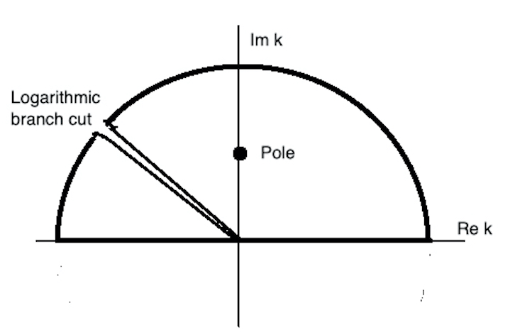
Figure 5: Sketch of the Integration contour for the inverse Fourier transform. of Eq.(31)

The residue at the complex pole ${\hat{V}}(kb)/\Theta=-1$ would lead to an exponential shielding analogous to the Debye shielding for a particle plasma. The integral along the two sides of the logarithmic branch-cut would lead to a non exponential contribution not present in a particle plasma.

These qualitative statements are confirmed by integrating Eq.(31) numerically for different values of the dimensionless temperature $\Theta$. In Fig.6 we show the result of this integration for $\Theta=2$.

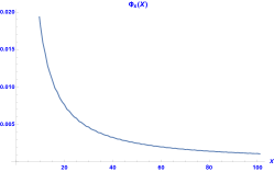
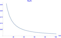
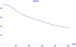
Figure 6: Plot of the screened potential $\Phi_{s}(X)$ in Eq.(31) as a function of $X=x/d$: left frame in the interval $0-X-100$, center frame enlargement in the in the interval $0-X-10$ and right frame in the interval $0-X-1$. The integration over $\kappa$ has been limited to the interval, $0$-$15$ while the label $100$ on the horizontal axis refers to the number of points in $X$ for which the numerical integration has been performed.

In agreement with the potential ${V}(\xi)$ in Eq.(2), the shielded potential $\Phi_{s}(X)$ is finite and nearly constant at $X\sim 0$ as shown in the enlarged plot in the right frame. For larger values of $X$ the potential $\Phi_{s}(X)$ has a fast exponential-type decay. Afterwards, as already visible in the central frame, the spatial dependence of the screened potential changes to a slower power-like decay, as shown by the full plot in the left frame. The exponent of this power law decrease is marginally larger in absolute value than $1$, i.e. marginally faster than the non-shielded potential.

4 Cold disk plasma waves

We consider the case where the disk thermal motion can be neglected and derive the linear dispersion relation of the cold disk plasma waves using Eqs.(5,6,7,8).

Linearization for a monochromatic wave in a stationary equilibrium with density $n_{0}$ and immobile ion-disks yields

$${\tilde{u}_{e}}=\frac{{\tilde{n}}_{e}}{n_{o}}\frac{\omega}{k},\qquad{\tilde{u}_{e}}=\frac{4k{\tilde{n}}_{e}}{M_{e}\omega}\,Q^{2}{\hat{V}}(kb),$$ (32)

which gives

$$\omega^{2}=\omega_{Dpe}^{2}\,[(kb)^{2}\,{\hat{V}}(kb)],\quad{\rm where}\quad\omega_{Dpe}^{2}=\frac{4Q^{2}n_{o}}{M_{e}b^{2}}.$$ (33)

We see that the disk-plasma waves are dispersive for finite values of $kb$. In the short wavelength limit $kb\gg 1$ the waves become Langmuir waves (see Note 1 and Eq.(49), Appendix A) with frequency $\omega_{Dpe}$ where $n_{o}/(\pi b^{2})$ has the dimension of a volume density.
In the long wavelength limit (see Appendix A, Eq.(A) which defines the constants $C_{1},\,C_{2}$) we find (logarithmically corrected) “cold electron-disk sound” waves of the form

$$\omega^{2}=k^{2}[C_{1}+C_{2}\ln{(kb)^{2}}]v^{2}_{D},\quad{\rm where}\quad v^{2}_{D}=b^{2}\omega_{Dpe}^{2}=\frac{4Q^{2}n_{o}}{M_{e}}.$$ (34)

We note that in a particle plasma there is no velocity directly corresponding to $v_{D}$.
The phase velocity of Langmuir waves is smaller than $v_{D}$ as follows from $\omega^{2}/k^{2}=\omega_{Dpe}^{2}/k^{2}=v^{2}_{D}/(kb)^{2}<<v^{2}_{D}$ while in the case of the cold sound waves we have $\omega^{2}/k^{2}\sim[\ln(kb)]^{2}v_{D}^{2}>>v_{D}^{2}$.

5 Disk Vlasov equation and waves

The treatment of the Vlasov kinetic equation follows standard lines with two minor differences: the expression of the interaction potential $V(\xi)$ is different from the Coulomb potential and it is more convenient to use the particle density as the independent variable instead of the potential Thus we have the integro-differential equation

$$\frac{\partial{f}_{j}(x,v,t)}{\partial t}+v\frac{\partial{f}_{j}(x,v,t)}{\partial x}+\frac{{{\cal F}}_{j}(x,t)}{M_{j}}\frac{\partial{f}_{j}(x,v,t)}{\partial v}=0$$ (35)

where ${f}_{j}(x,v,t)$ is the distribution function of the $j$ species ($j=e,i$), $v$ is the disk velocity coordinate in phase space and ${\cal F}_{j}(x,t)$ is defined in Eq.(7)] and

$${\rho}(x,t)=Q\left[\int_{-\infty}^{+\infty}{f}_{i}(x,v,t)\,dv-\int_{-\infty}^{+\infty}{f}_{e}(x,v,t)\,dv\right].$$ (36)

5.1 Linearized equation

In a homogeneous disk plasma the linearized Vlasov equation takes the form

$$\frac{\partial{\tilde{f}}_{j}(x,v,t)}{\partial t}+v\frac{\partial{\tilde{f}}_{j}(x,v,t)}{\partial x}+\frac{{\tilde{\cal F}}_{j}(x,t)}{M_{j}}\frac{\partial{f}_{j0}(v)}{\partial v}=0$$ (37)

where ${f}_{j0}(v)$ and ${\tilde{f}}_{j}(x,v,t)$ are the equilibrium and the perturbed distribution functions, $v$ is the disk velocity and

$${\tilde{\cal F}}_{j}(x,t)=-4ikQ_{j}{\hat{\rho}}(k){\hat{V}}(kb),$$ (38)

is the perturbed force, as obtained from Eq.(23).
Considering again for the sake of simplicity immobile ion disks and waves of the form

$${\tilde{f}}_{e}(x,v,t)={\tilde{f}}_{o}(v)\exp{[-i(\omega t-kx)]},\qquad{\tilde{\rho}}(x,t)={\tilde{\rho}}_{o}\,\exp{[-i(\omega t-kx)]}$$ (39)

$${\rm with}\quad{\tilde{\rho}}_{o}=-Q{\tilde{n}}_{eo}=-Q\int_{-\infty}^{+\infty}{\tilde{f}}_{eo}(v)\,dv,$$

we obtain the dispersion relation

$$1=-4kQ^{2}\frac{{\hat{V}}(kb)}{M_{e}}\int_{-\infty}^{+\infty}\frac{\partial{f}_{eo}(v)/\partial v}{\omega-kv}\,dv=-\frac{\omega_{Dpe}^{2}}{k}[(kb)^{2}{\hat{V}}(kb)]\int_{-\infty}^{+\infty}\frac{\partial[{f}_{eo}(v)/n_{o}]/\partial v}{\omega-kv}\,dv,$$ (40)

where the velocity integral has to be taken according to the Landau prescription. In the cold limit when $\omega/k\gg v_{the}$, with $v_{the}$ the halfwidth of the distribution function ${\tilde{f}}_{eo}$, Eq.(40) becomes

$$1=4Q^{2}n_{o}\frac{k^{2}}{\omega^{2}}\frac{{\hat{V}}(kb)}{M_{e}}=\frac{\omega_{Dpe}^{2}}{\omega^{2}}[(kb)^{2}{\hat{V}}(kb)],$$ (41)

which coincides with Eq.(33).

The dispersion relation given by Eq.(40) depends on the normalized wave number $kb$ and in addition on the equilibrium dimensionless parameter $(v_{the}/v_{D})^{2}=\Theta$ (see below Eq.(3.1)). For disk-Langmuir waves the cold limit $\omega/k\gg v_{the}$ implies $v_{the}/v_{D}\ll 1/(kb)\ll 1$, whereas for cold sound waves it implies the less restrictive condition $v_{the}/v_{D}\ll|\ln{(kb)^{2}}|$ where $|\ln{(kb)^{2}}|\gg 1$ .

Normalizing velocities over $v_{D}$, Eq. (40) can be rewritten in terms of ${\bar{\omega}}=\omega/\omega_{Dpe}$,   ${\bar{v}}=v/v_{d}$ and $\kappa=kb$ as

$$1=-\kappa{\hat{V}}(\kappa)\int_{-\infty}^{+\infty}\frac{\partial{\bar{f}}_{eo}({\bar{v}})/\partial{\bar{v}}}{{\bar{\omega}}-\kappa{\bar{v}}}\,{d\bar{v}}\ ,$$ (42)

where the dimensionless distribution function ${\bar{f}}_{eo}({\bar{v}})=v_{D}f_{eo}(v)/n_{o}$ depends on the dimensionless temperature   $\Theta=T_{e}/(4Q^{2}n_{o})$.

6 Conclusions

In order to model collective electrostatic effects on a 3-D plasma using a reduced dimensionality configuration, it may be convenient to define an effective interaction energy constructed so as to retain the physical effects that we deem must be included in order to to construct a “faithful” model.
In these notes we have introduced a model of interacting charged disks that provides a one-dimensional model with an interaction energy that vanishes at infinity.

Clearly this approach is restricted to the case where the system evolution may be described by “scalar one-dimensional electrodynamics”, i.e. when no magnetic fields are present and the electric field is the gradient of a one-dimensional scalar potential.

Appendix A Disks electrostatics

A set of relevant formulae derived in Ref.[5] are listed below along with some notational adaptations.

The axially symmetric electrostatic potential $\varphi(r,x)$ created by a uniformly charged disk with its center at the coordinate origin, with total charge $Q$ and radius $b$ can be written as

$$\varphi(r,x)=2Q\int_{0}^{+\infty}dsJ_{o}(sr)\frac{J_{1}(sb)}{sb}\exp{(-s|x|)},$$ (43)

where $J_{0}$ and $J_{1}$ are are Bessel functions, while the $x$-component of the electric field can be written as

$${\epsilon}_{x}(r,x)={\rm sign(x)}\,\frac{2Q}{b}\int_{0}^{+\infty}dsJ_{o}(sr)J_{1}(sb)\,\exp{(-s|x|)},$$ (44)

which, at $r=0$, reduces to

$${\epsilon}_{x}(0,x)={\rm sign(x)}\,\frac{2Q}{b}\int_{0}^{+\infty}dsJ_{1}(sb)\,\exp{(-s|x|)}={\rm sign(x)}\,\frac{2Q}{b^{2}}\left[1-\frac{|x|/b}{(1+x^{2}/b^{2})^{1/2}}\right].$$ (45)

The expression for the interaction energy in Eq.(1) is the result of the integral

$${\cal W}(|x|)=4\frac{Q_{1}\,Q_{2}}{b}V(|x|/b)=\frac{4Q_{1}Q_{2}}{b}\int_{0}^{+\infty}ds[J_{1}(s)/s]^{2}\,\exp{(-s|x|/b)},$$ (46)

which is obtained by integrating Eq.(43) over the disk surface.

The Fourier transform of $V(\xi)$ can be obtained from the equation above in the form

$${\hat{V}}(kb)=\int_{-\infty}^{+\infty}\frac{dx}{b}\,V(|x|/b)\exp{-[i(kb)\,(x/b)]}=$$ (47)

$$\int_{0}^{+\infty}ds[J_{1}(s)/s]^{2}\,\int_{-\infty}^{+\infty}\frac{dx}{b}\,\exp{(-s|x|/b)}\exp{-[i(kb)\,(x/b)]}=$$

$$2\int_{0}^{+\infty}ds[J_{1}(s)/s]^{2}\,\int_{0}^{+\infty}\frac{dx}{b}\,\exp{(-sx/b)}\cos{[(kb)\,(x/b)]}=$$

$$2\int_{0}^{+\infty}ds[J_{1}(s)/s]^{2}\,\frac{s}{(kb)^{2}+s^{2}}=\frac{1}{\pi^{1/2}(kb)^{2}}G^{2,2}_{2,4}\left((kb)^{2}\left|{}^{1/2,1}_{1,1,-1,0}\right.\right)$$

where Meijer $G^{2,2}_{2,4}$ is a Meijer G function [7], denoted as $G$-Function in the notation used by “Mathematica” (see https://reference.wolfram.com/language/ref/MeijerG.html)

$${\rm Meijer}G[\{\{a_{1},a_{2}\},\{...\}\},\{\{b_{1},…,b_{2}\},\{b_{3},b_{4}\}\},z]=G^{2,2}_{2,4}\left(z\left|{}^{a_{1},a_{2}}_{b_{1},b_{2},b_{3},b_{4}}\right.\right)$$

The function $G^{2,2}_{2,4}\left((kb)^{2}\left|{}^{1/2,1}_{1,1,-1,0}\right.\right)/\left[2(\pi^{1/2}(kb)^{2})\right]$ has the following limits (as given by “Mathematica” )

$$\frac{1}{\pi^{1/2}(kb)^{2}}G^{2,2}_{2,4}\left((kb)^{2}\left|{}^{1/2,1}_{1,1,-1,0}\right.\right)=(1/8)\left[5-6\gamma-2\ln{[(kb)^{2}]}-2\psi(3/2)\right]$$

$$+(1/48)\left[13-9\gamma-3\ln{[(kb)^{2}]}-3\psi(5/2)\right](kb)^{2}$$

$$+(5/92316\left[-65+36\gamma+12\ln{[(kb)^{2}]}+12\psi(7/2)\right](kb)^{4}+...,$$ (48)

for $(kb)^{2}\ll 1$ , where $\gamma=0.577216$, $\psi(z)=d\ln{\Gamma(z)}/dz$, and

$$G^{2,2}_{2,4}\left((kb)^{2}\left|{}^{1/2,1}_{1,1,-1,0}\right.\right)=\pi^{1/2}+....$$ (49)

for $(kb)^{2}\gg 1$. In this latter limit we recover the standard Coulomb-like dependence ${\hat{V}}\propto 1/k^{2}$.
The logarithmic dependence at small wavenumbers arises from the $1/x$ dependence of the interaction energy at large distances in 1-D.

References

[1]
P.J. Morrison, F Pegoraro, On the Hamiltonian structure of the BBGKY hierarchy, 63rd Annual Meeting of the APS Division of Plasma Physics, UP11.00040 (2021).
[2] N.A. Krall, A.W. Trivelpiece, Principles of plasma physics, (San Francisco Press, San Francisco, CA) 1986.
[3] N. N. Bogoliubov, Kinetic Equations, Journal of Physics USSR, 10, 265 (1946).
[4] J. E. Marsden, P. J. Morrison, A. Weinstein, The Hamiltonian Structure of the BBGKY Hierarchy Equations, Contemporary Mathematics , 28, 115 (1984).
[5] O. Ciftja,
Electrostatic interaction energy between two coaxial parallel uniformly charged disks,
Results in Physics, 15, 102684 (2019),
https://doi.org/10.1016/j.rinp.2019.102684.
[6] M. Abramowitz , I. A. Stegun, Handbook of Mathematical Functions with Formulas, Graphs, and Mathematical Tables,
(Dover, New York, 1964).
[7]NIST Digital Library of Mathematical Functions, https://dlmf.nist.gov/