Random Access Protocol with Channel Oracle Enabled by a Reconfigurable Intelligent Surface

Abstract

The widespread adoption of Reconfigurable Intelligent Surfaces (RISs) in future practical wireless systems is critically dependent on the integration of the RIS into higher-layer protocols beyond the physical (PHY) one, an issue that has received minimal attention in the research literature. In light of this, we consider a classical random access (RA) problem, where uncoordinated users’ equipment (UEs) transmit sporadically to an access point (AP). Differently from previous works, we ponder how a RIS can be integrated into the design of new medium access control (MAC) layer protocols to solve such a problem. We consider that the AP is able to control a RIS to change how its reflective elements are configured, namely, the RIS configurations. Thus, the RIS can be opportunistically controlled to favor the transmission of some of the UEs without the need to explicitly perform channel estimation (CHEST). We embrace this observation and propose a RIS-assisted RA protocol comprised of two modules: Channel Oracle and Access. During channel oracle, the UEs learn how the RIS configurations affect their channel conditions. During the access, the UEs tailor their access policies using the channel oracle knowledge. Our proposed RIS-assisted protocol is able to increase the expected throughput by approximately 60% in comparison to the slotted ALOHA (S-ALOHA) protocol.

I Introduction

Reconfigurable Intelligent Surfaces (RISs) are low-power wireless system elements that can shape the radio waves to enable smart radio environments [1, 2]. The majority of the literature on RIS-assisted communication systems has predominantly focused on the physical (PHY) layer aspects, including the modeling of the related electromagnetic phenomena [3, 4]. Many papers have shown potential benefits in terms of spectral and energy efficiencies of RIS-assisted systems [5], which are based on the development of optimization methods for the RIS alone or jointly with the access point (AP) precoding [6, 7, 8]. Because of this, several works have focused on the design and evaluation of channel estimation (CHEST) procedures in the presence of RIS [9]. A particular effort has been made to reduce the overhead of CHEST, which can be very high due to the high number of elements that compose the RIS [10, 11, 12]. However, in general, less attention has been paid to integrating the RIS into protocols at higher layers to leverage the PHY benefits provided by the RIS.

An interesting first problem for the integration of the RIS into higher layers is to consider the random access (RA) problem or the “free-for-all” multiaccess communication [13, 14], where individual resource allocation and coordination among users equipment (UEs) are not feasible. The interesting questions here are $i$) How to coordinate transmissions to avoid collisions so that exactly one UE is transmitting for a given time period? and $ii$) When and how to retransmit packets when collisions occur? Another complicating factor is that the AP just know the area where the UEs are placed. Conventionally, these issues are addressed at the medium access control (MAC) layer, which implements protocols to allocate the multiaccess medium among UEs [13, 14]. In particular, we refer to an RA protocol as a distributed algorithm whose common objective is to solve the aforementioned questions.

Legacy MAC protocols are often designed by taking only APs and UEs as communication nodes, such as in slotted ALOHA (S-ALOHA) [13, 14]. However, by introducing the RIS into the environment, the shared channel is definitely affected. To see this, consider a typical wireless multiaccess channel, where the received signal at the AP is the sum of attenuated transmitted signals from a set of UEs, with the signals being corrupted by distortion, delay, and noise [13]. In a RIS-assisted wireless multiaccess channel, the signals of some of these UEs can be intentionally favored over others due to the RIS’ reflecting capabilities without the need to explicitly perform CHEST. In particular, we are interested in the case that an AP controls a RIS by being able to change how the reflective elements that compose the RIS are configured, namely, the RIS configurations. Each of the RIS configurations directs an incoming wave in a specific direction, called the reflected angular direction or reflection angle. In this paper, we propose a RIS-assisted RA protocol that distills the above insight by separating the UE transmissions in time based on their geographical location and the design of RIS configurations, allowing the UEs to opportunistically determine the adequate time to transmit by running an algorithm locally.

I-A Related Works

For RIS-assisted wireless systems, there is a gap in the literature regarding the RA and related problems. The authors of [8, 15] present designs for MAC protocols that integrate RISs for multi-user communications. These works address the multiaccess problem based on the “perfectly scheduled” approach [13], where the APs already know the UEs because they have been scheduled somehow. This is conceptually different from the RA problem being addressed here, where the latter is more challenging since few things are known among communication nodes. For example, the RA problem precedes the CHEST, since scheduling had not been realized yet. In this regard, a closely related work is [16], where the authors consider the activity detection problem for unsourced RA by using the RIS to improve the channel quality and control channel sparsity. However, this work does not clarify how to adequately integrate the RIS into the protocol design and uses the PHY controlling capabilities of RIS only as an artifact to improve channel sparsity under very specific operating conditions, such as the use of millimeter waves. In addition, the authors in [17] propose an activity detection algorithm that optimizes the RIS configuration to obtain optimal detection probability. However, the procedure relies on a partial CHEST. In [18], the authors analyze the performance of a RIS-assisted RA using successive interference cancellation (SIC) for uncoordinated transmission attempts from two transmitters demonstrating that the RIS can help achieve better performance due to increased signal-to-noise ratio (SNR). Nevertheless, the work also lacks the systematical aspects behind a protocol. To address these problems, in [19], we have proposed a proof-of-concept of the RIS-assisted RA protocol that is going to be shown here. In there, we have shown substantial gains in integrating the RIS into the RA protocol design. Still, we have omitted several engineering details of the protocol, important for the overall system design.

I-B Contributions

Our proposed RIS-assisted RA protocol is based on the observation that the AP can control the RIS to intentionally favor the transmission of some of the UEs without the need of CHEST. Naturally, one might think that because of this the RIS might act as a mediator or coordinator in a completely uncoordinated environment bringing some light into the darkness. However, for this coordination to be possible, we had the idea that UEs need to be aware of when they are being favored. That is, they need to know how their channels change w.r.t. the reflected angular space spanned by the RIS configurations. Thus, our protocol comprises two modules: A. Channel Oracle and B. Access. During the channel oracle, each UE learns when and how its channel is favored by the RIS considering its current positions. During access, each UE exploits the channel oracle knowledge to come up with a tailored access policy that can be designed to define when to retransmit packets and to avoid collisions. Our proposed RIS-assisted RA protocol has several compelling advantages: it improves overall MAC performance in comparison with legacy protocols, it encourages the installation of RISs instead of new APs, which could end up to be cheaper and more energy efficient, and it provides the AP with relevant information to conduct other operations that start after the RA. For example, it can alleviate the computational complexity of CHEST, since the access policies, if properly designed, tend to reveal information about where UEs are located and their channel conditions.

The remainder of the paper is organized as follows. In Section II, we introduce our system model by setting up all that is need for the presentation of the protocol. In Section III the protocol is presented more broadly. We give particular details on how to design the Channel Oracle and Access modules in Sections IV and V, respectively. In Section VI, we discuss several practical details of the protocol and how they can be extended to some other system models and set of assumptions. Finally, we numerically evaluate our protocol in Section VII, whereas Section VIII draws our main conclusion.

Notations. The set of positive integers, positive real, real, and complex numbers are denoted by $\mathbb{Z}_{+}$, $\mathbb{R}_{+}$, $\mathbb{R}$, and $\mathbb{C}$, respectively. Integer sets are denoted by calligraphic letters $\mathcal{A}=\{0,1,\dots,A-1\}$ with cardinality $|\mathcal{A}|=A$. The circularly-symmetric complex Gaussian distribution is $\mathcal{N}_{\mathbb{C}}(\mu,\sigma^{2})$ w/ mean $\mu$ and variance $\sigma^{2}$. Lower and upper case boldface letters denote column vectors $\mathbf{x}$ and matrices $\mathbf{A}$, respectively. The identity matrix of size $N$ is $\mathbf{I}_{N}$ and $\mathbf{0}$ is a vector of zeros of arbitrary size. Euclidean norm is $\lVert\mathbf{x}\rVert_{2}$. Superscript $(\cdot)^{*}$ denotes complex conjugate. The $\arg\max(\cdot)$ function returns the index of the maximum element of a vector, while $\mathrm{med}\{\cdot\}$ and $\mathrm{max}\{\cdot\}$ denote the median and the maximum operator over a set, respectively.

II System Model

Consider the wireless local area network depicted in Fig. 1, which is comprised of one single-antenna AP, one RIS, and multiple $K\in\mathbb{Z}_{+}$ single-antenna UEs, which are indexed by the set $\mathcal{K}$. We assume that the AP does not have any prior knowledge of the UEs. This scenario may correspond to an industrial installation, where many sensors and actuators with wireless communication capabilities communicate with an AP of a network infrastructure. For example, the AP can be deployed outside, while the UEs are located within an industrial shed. However, due to possible blockages, such as machines and walls, the line-of-sight (LoS) paths among the AP and the UEs are blocked. In this context, the network operator may decide to install a RIS to improve the quality of the communication among the AP and the UEs, instead of installing a new AP within the shed. Note that it is reasonable to assume only one RIS since we are dealing with a very controlled application scenario. However, multiple RISs can be considered, where each RIS helps the communication of different sets of geographically isolated UEs; e.g., located in several sheds. Moreover, we consider that the AP controls the operation of the RIS through a dedicated out-of-band control channel (CC), i.e., controlling the RIS does not interfere with the wireless signals exchanged among the AP and UEs [5]. For convenience, we also assume that the CC is error-free with the command messages sent by the AP being perfectly interpreted by the RIS controller (RIS-C) at the RIS’ side.

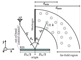
Figure 1: Two-dimensional view of the considered system setup assisted by a RIS of negligible thickness.

To keep the complexity of the analysis at a minimum while showing the working principles of the proposed RIS-assisted RA protocol, we will analyze the performance of the system under the following assumptions.

Assumption 1 (Ideal RIS).

The considered RIS is assumed to have an ideal hardware able to induce a stable phase shift on the incident wave without affecting its amplitude, and with negligible mutual coupling among reflecting elements.

Assumption 2 (UEs Positioning).

The AP and the UEs are located on the $x$-$y$ plane having $z$-coordinate equal to 0, i.e., they lay on the same plane of the center of the RIS.

In a real implementation, the RIS’ reflecting elements, or simply elements, generate an attenuation loss which is a function of the selected phase shift [20, 21]. Moreover, each element can only induce a phase shift whose value comes from a finite set [6] due to hardware constraints. Finally, inter-element coupling effects might exist [22], while usually assumed negligible [5, 23]. Thus, the results provided in this paper can be seen as an upper bound in terms of performance since attenuation, finite precision, and mutual coupling would result in performance losses. On the other hand, constraining the position of the UEs on the same plane allows us to present the protocol structure analyzing the problem as a function of the incident angle only, i.e., in a single angular dimension. Thus, Assumptions 1 and 2 yield a simple analytical model that can be exploited to clearly present the main, new ideas behind the proposed RIS-assisted RA protocol. We discuss possible directions on how to extend the protocol to other scenarios with a different set of assumptions in Sect. VI.

II-A Geometry

As illustrated in Fig. 1, the RIS is positioned in such a way that it can reflect signals transmitted by the AP into the area where the UEs are located and vice versa. The center of the RIS is the origin of our coordinate system. The RIS is formed by $M_{x}\in\mathbb{Z}_{+}$ and $M_{z}\in\mathbb{Z}_{+}$ elements arranged in a planar array over the $x$- and $z$-dimensions, with index sets $\mathcal{M}_{x}$ and $\mathcal{M}_{z}$, respectively, and totaling $M=M_{x}M_{z}$ elements. Each wavelength-scale element is realized as a metalized layer on a grounded substrate and has an area of $d_{x}d_{z}$ with $d_{x},d_{z}\in\mathbb{R}_{+}$ and $d_{x},d_{z}\leq\lambda$, where $\lambda$ is the wavelength of the carrier signal. The dimensions of the RIS are $D_{x}=M_{x}d_{x}$ and $D_{z}=M_{z}d_{z}$. Following Assumption 2, we denote as $\theta_{a}\in[0,{\pi}/{2}]$ the angle between the line normal to the origin and the AP, and as $\theta_{k}\in[0,{\pi}/{2}]$ the equivalent angle w.r.t. the $k$-th UE, $\forall k\in\mathcal{K}$. The corresponding distances are denoted as $d_{a}$ and $d_{k}\in[d_{\min},d_{\max}]$, where $d_{\min}$ and $d_{\max}$ denote the minimum and maximum distances, respectively. The minimum distance is set as $d_{\min}=\frac{2}{\lambda}\max(D_{x}^{2},D_{z}^{2})$ so that we can analyze the electromagnetic signals reflected by the RIS in the far-field regime [24], assuring the assumption of plane-wave propagation. The maximum distance $d_{\max}$ stipulates the lower boundaries of the SNR range, i.e., it is set as the maximum distance the RIS is able to provide a sufficient good SNR at the UEs.

II-B RIS Configurations

According to Assumption 1, we let $\phi_{m,m^{\prime}}\in[0,2\pi],\,\forall m\in\mathcal{M}_{x},\ \forall m^{\prime}\in\mathcal{M}_{z}$ denote the phase shift impressed by the $(m,m^{\prime})$-th element. Without loss of generality, we assume a transverse electromagnetic mode propagation [24], where the electromagnetic waves propagate within the plane perpendicular to the $z$-axis [6]. Consequently, and in agreement with Assumption 2, the RIS’ elements with the same index over the $z$-dimension impress the same phase shift, to maximize the energy on the $x-y$ plane. Hence, for notation convenience, the dependency with the $z$-dimension can be dropped as $\phi_{m,m^{\prime}}=\phi_{m,m^{\prime\prime}}=\phi_{m},\,\forall m^{\prime},m^{\prime\prime}\in\mathcal{M}_{z}$. We then refer to a vector of phase shifts $\bm{\phi}\in[0,2\pi]^{M_{x}M_{z}}$ as a RIS configuration denoting a particular way in which the reflective elements of the RIS are configured to scatter the incoming wave. In our context, we consider that the RIS has a finite number $N\in\mathbb{Z}_{+}$ of predefined configurations collected in the so-called RIS configuration codebook $\Phi=\{\bm{\phi}[n]\}_{n\in\mathcal{N}}$, where $\mathcal{N}$ is the index set and $[n]$ is used for indexing as a notation convenience based on classical signal processing literature [25]. We note that the RIS configuration codebook $\Phi$ can be comprised of many subsets $\Phi_{i}$, where each configuration codebook can be designed for a particular task. During the network setup, the configuration codebook $\Phi$ is loaded into the AP and RIS hardware. During the network operations, the AP controls the behavior of the RIS by referring to configurations of $\Phi$.

From Reflection Angles to Configurations. Each configuration can be related to the angle of the resulting reflected wave, denoted as $\theta^{\rm\scriptscriptstyle{DL}}_{r},\theta^{\rm\scriptscriptstyle{UL}}_{r}\in[0,{\pi}/{2}]$, for downlink (DL) and uplink (UL) directions, respectively. Mathematically, let $h:\Theta\mapsto\Phi$ be the bijective mapping among reflection angles and configurations. We now analyze how to design a configuration codebook having in view the reflection angles and the facts that the AP controls the RIS and does not have prior knowledge of the UEs’ positions when wishing to enable RA functionalities. In the DL, suppose that the AP sends a signal toward the RIS, whose incoming direction is $\theta_{a}$. The AP can control the RIS to reflect the incoming wave toward a desired DL angular direction $\theta^{\rm\scriptscriptstyle{DL}}_{r}$. In our context, the AP wishes to sense a particular angular direction looking for UEs, that is, it would like to choose a DL reflection direction $\theta^{\rm\scriptscriptstyle{DL}}_{r}$ that matches with a $\theta_{k},\,k\in\mathcal{K}$. In other words, the reflection angle $\theta^{\rm\scriptscriptstyle{DL}}_{r}$ is chosen blindly by the AP with the intention of matching with the angular position of a UE since the AP does not know the UEs’ angular positions $\theta_{k}$. Now, in the UL, suppose that a single or multiple UEs transmit, meaning that the incoming signal(s) from the RIS’s standpoint comes from random directions $\theta_{k}$. Since the AP controls the RIS, the best the AP can guess is that the incoming waves are coming from the reflection directions $\theta^{\rm\scriptscriptstyle{DL}}_{r}$’s used during the DL instead of $\theta_{k}$’s. This consequently interlaces both the DL and UL phases. The AP can then control the RIS to reflect the incoming waves toward a desired UL angular direction $\theta^{\rm\scriptscriptstyle{UL}}_{r}$. Naturally, the AP controls the RIS to reflect the scattered incoming waves toward itself, i.e., $\theta^{\rm\scriptscriptstyle{UL}}_{r}=\theta_{a}$. Based on this, the configuration design from reflection angles to configurations can be written as [26]:

$$\phi^{\rm\scriptscriptstyle{DL}}_{m} =\omega\,d_{x}\,(m+1)(\sin\theta_{a}-\sin\theta^{\rm\scriptscriptstyle{DL}}_{r}),\text{ and}$$

$$\phi^{\rm\scriptscriptstyle{UL}}_{m} =\omega\,d_{x}\,(m+1)(\sin\theta^{\rm\scriptscriptstyle{DL}}_{r}-\sin\theta_{a}),$$ (1)

where $\phi^{\rm\scriptscriptstyle{DL}}_{m}$ and $\phi^{\rm\scriptscriptstyle{UL}}_{m}$ are the phase shifts impressed at the $m$-th element under DL and UL transmissions, respectively, $\forall m\in\mathcal{M}_{x}$. Given that we have $N$ configurations, we can denote the DL and UL the bijective mappings as $\bm{\phi}^{\rm\scriptscriptstyle{DL}}[n]=h^{\rm\scriptscriptstyle{DL}}(\theta^{\rm\scriptscriptstyle{DL}}_{r}[n])$ and $\bm{\phi}^{\rm\scriptscriptstyle{UL}}[n]=h^{\rm\scriptscriptstyle{DL}}(\theta^{\rm\scriptscriptstyle{UL}}_{r}[n])$, respectively. Note that from the general case above $\phi^{\rm\scriptscriptstyle{DL}}_{m}=-\phi^{\rm\scriptscriptstyle{UL}}_{m}$ since $\theta^{\rm\scriptscriptstyle{UL}}_{r}=\theta_{a}$, meaning that the corresponding mappings are related as $h^{\rm\scriptscriptstyle{DL}}(\theta^{\rm\scriptscriptstyle{DL}}_{r})=(h^{\rm\scriptscriptstyle{UL}}(\theta^{\rm\scriptscriptstyle{UL}}_{r}))^{*}$. Thus, since the DL configuration is just the complex conjugate of the UL one due to channel reciprocity, the AP and RIS can just agree on a ”unidirectional” configuration codebook $\Phi$ and the AP signalizes either if the configuration should be complexly conjugated, indicating UL, or not for DL.

II-C RIS-Assisted Slotted Multiaccess

Consider a standard frame structure of data link control (DLC), where each frame represents the data stream that a single UE wants to transmit toward the AP. A frame has fixed duration $T_{\rm F}\in\mathbb{R}_{+}$, comprises a cyclic redundancy check (CRC) for error detection, while stop-and-wait automatic repeat request (ARQ) is used for error correction. For PHY transmission, this frame is sliced into transmission packets. Assume a slotted system for transmission over the PHY layer, where all transmitted packets have the same duration $T_{\rm s}\in\mathbb{R}_{+}$ and each packet requires a one-time unit or slot for transmission. Thus, the overall frame duration is $T_{\rm F}=N_{\rm F}T_{s}$, where $N_{\rm F}\in\mathbb{Z}_{+}$ is the number of slots in a frame. Moreover, we consider that each slot is further sliced into $L\in\mathbb{Z}_{+}$ samples or symbols with fixed symbol duration $T_{\rm symb}\in\mathbb{R}_{+}$; hence, $T_{s}=LT_{\rm symb}$. Conventionally, the multiaccess problem culminates in coordinating the use of the slotted PHY channel so to avoid collisions among UEs on a slot basis. However, now we have a controllable channel due to the RIS, leading to new approaches to attain some coordination among UEs. We are interested in studying these new possibilities and for this, we assume the following.

Assumption 3 (Slotted Configuration Change).

The AP can control the RIS to change its configurations on a slot basis, where a single configuration can be changed per slot. Therefore, at the beginning of each slot, the AP sends a configuration change command to the RIS. After the RIS receives this command, it needs a certain time to physically load the new configuration. We let $T_{\rm sw}\in\mathbb{R}_{+}$ be the switching time, i.e., the time the RIS requires to switch to a new configuration. The AP remains silent during $T_{\rm sw}$ in the DL and ignores any signal received during the switching time in the UL. Note that $T_{\rm sw}$ can also incorporate the time spent on sending command messages over the CC.

II-D Physical Channel Model

Assume dominant LoS paths for AP to RIS and RIS to a UE $k$. The DL channel coefficient $\zeta_{k}^{\rm\scriptscriptstyle{DL}}(\bm{\phi}^{\rm\scriptscriptstyle{DL}})\in\mathbb{C}$ is:

$$\zeta_{k}^{\rm\scriptscriptstyle{DL}}(\bm{\phi}^{\rm\scriptscriptstyle{DL}}) =\sqrt{\beta_{k}^{\rm\scriptscriptstyle{DL}}}e^{j\omega\psi_{k}}\mathrm{A}_{k}(\bm{\phi}^{\rm\scriptscriptstyle{DL}})\text{ with}$$ (2)

$$\beta_{k}^{\rm\scriptscriptstyle{DL}} =\dfrac{G_{a}G_{k}}{(4\pi)^{2}}\left(\dfrac{d_{x}d_{z}}{d_{a}d_{k}}\right)^{2}\cos^{2}\theta_{a},$$ (3)

where $(\bm{\phi}^{\rm\scriptscriptstyle{DL}})$ denotes the dependency on the phase shifts, $\beta_{k}^{\rm\scriptscriptstyle{DL}}\in\mathbb{R}_{+}$ is the DL pathloss with $G_{a}$ and $G_{k}$ being the antenna gain of the AP and of the UE, respectively. The propagation phase shift $\psi_{k}\in[0,2\pi]$ and the array factor arising from the discretization of the RIS into a finite number of elements are:

$$\psi_{k}=-\left(d_{a}+d_{k}-(\sin\theta_{a}-\sin\theta_{k})\frac{M_{x}+1}{2}d_{x}\right)\text{ and}$$ (4)

$$\mathrm{A}_{k}(\bm{\phi}^{\rm\scriptscriptstyle{DL}})=M_{z}\sum_{m\in\mathcal{M}_{x}}e^{j(\omega d_{x}(m+1)(\sin\theta_{k}-\sin\theta_{a})+\phi^{\rm\scriptscriptstyle{DL}}_{m})},$$ (5)

where $\phi^{\rm\scriptscriptstyle{DL}}_{m}\in[0,2\pi]$ is the $m$-th element of $\bm{\phi}^{\rm\scriptscriptstyle{DL}}$. Similarly, the UL channel coefficient $\zeta_{k}^{\rm\scriptscriptstyle{UL}}(\bm{\phi}^{\rm\scriptscriptstyle{UL}})\in\mathbb{C}$ and the corresponding pathloss $\beta_{k}^{\rm\scriptscriptstyle{UL}}\in\mathbb{R}_{+}$ are

$$\zeta_{k}^{\rm\scriptscriptstyle{UL}}(\bm{\phi}^{\rm\scriptscriptstyle{UL}}) ={\sqrt{\beta_{k}^{\rm\scriptscriptstyle{UL}}}}e^{-j\omega\psi_{k}}\mathrm{A}_{k}(\bm{\phi}^{\rm\scriptscriptstyle{UL}})\text{, and}$$ (6)

$$\beta_{k}^{\rm\scriptscriptstyle{UL}} =\dfrac{G_{a}G_{k}}{(4\pi)^{2}}\left(\dfrac{d_{x}d_{z}}{d_{a}d_{k}}\right)^{2}\cos^{2}\theta_{k}.$$ (7)

The interested reader can check more details about the derivation of the above model in [19]. It is worth pointing out that the antenna array model adopted here can be extended to include the near-field of the RIS through recently proposed plane wave expansion methods [4]. Note also that, by substituting (1) into (5), the array factor becomes:

$$\mathrm{A}_{k}(\bm{\phi}^{\rm\scriptscriptstyle{DL}})\equiv\mathrm{A}_{k}(\theta^{\rm\scriptscriptstyle{DL}}_{r})=M_{z}\sum_{m\in\mathcal{M}_{x}}e^{j\omega d_{x}(m+1)(\sin\theta_{k}-\sin\theta^{\rm\scriptscriptstyle{DL}}_{r})}.$$ (8)

Observe that $\mathrm{A}_{k}(\bm{\phi}^{\rm\scriptscriptstyle{UL}})=\mathrm{A}^{*}_{k}(\bm{\phi}^{\rm\scriptscriptstyle{DL}})$. As a result, the channel coefficients are also a function of the reflection angles, that is, it is equivalent to say that $\zeta^{\rm\scriptscriptstyle{DL}}_{k}(\bm{\phi}^{\rm\scriptscriptstyle{DL}})\equiv\zeta^{\rm\scriptscriptstyle{DL}}_{k}(\theta^{\rm\scriptscriptstyle{DL}}_{r})$. Due to the static or low mobility of the main scenario of interest and controllable scattering effects, the channel coefficients are assumed constant over slots.

III Proposed RIS-Assisted Random Access Protocol

In this section, we present the proposed RIS-assisted RA protocol illustrated in Fig. 2. The structure of the protocol is composed of two independent modules: $A$. Channel Oracle and $B$. Access. Inspired by the carrier sensing approach [13, 14], the basic idea of our protocol is that each UE can learn a model on how its channel coefficient varies over the reflected angular space spanned by the channel control offered by the RIS. The role of the channel oracle module is to specify how this learning task occurs in a distributed manner since the control of the RIS is owned by the AP and not by the UEs. By using the output of the channel oracle, the access module then specifies how the UEs attempt to transmit their packets to the AP over the multiaccess channel when considering that the AP is unaware of any prior information regarding the UEs and again owns the control of the RIS. We note that the access module depends on the output of the channel oracle module, otherwise, the UEs would not benefit from the environment control brought by the RIS. In this case, the access module could be simply replaced by legacy protocols, such as S-ALOHA [13, 14]. Moreover, one should keep in mind that the access module is realized much more often than the channel oracle one in practice. More practical details of the protocol can be seen in Section VI. Below we give an overview of the protocol modules and introduce performance metrics.

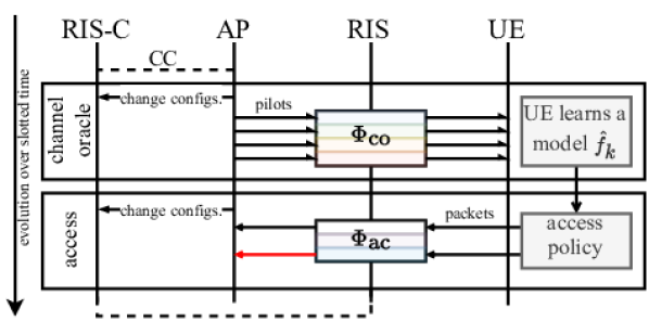
Figure 2: Time diagram of the proposed RIS-assisted RA protocol. The RIS-C denotes the RIS controller, which is connected to the AP via the CC. Operations occur sequentially in time following the top-down direction. The protocol is comprised of two modules: channel oracle and access. During the channel oracle, the AP sends pilots, while the RIS sweeps through a set of configurations $\Phi_{\rm co}$; this enables the UE to learn a model $\hat{\zeta}^{\rm\scriptscriptstyle{DL}}_{k}=\hat{f}_{k}(\theta^{\rm\scriptscriptstyle{DL}}_{r})$. During access, the UE exploits $\hat{f}_{k}$ to design access policies so that they can choose when to send packets, while the RIS sweeps again through another set of configurations $\Phi_{\rm ac}$. The red arrow illustrates a collision since hypothetically another UE decided to send a packet during the same access configuration.

III-A Channel Oracle

Mathematically, the channel oracle at the UE’s side consists of each UE $k$ learning a model $\hat{f}_{k}:[0,\pi/2]\mapsto\mathbb{C}$ of the channel such that $\hat{\zeta}^{\rm\scriptscriptstyle{DL}}_{k}=\hat{f}_{k}(\theta^{\rm\scriptscriptstyle{DL}}_{r})$, where the input is a DL reflection angle $\theta^{\rm\scriptscriptstyle{DL}}_{r}$ and the output is the DL estimated channel coefficient $\hat{\zeta}^{\rm\scriptscriptstyle{DL}}_{k}$, for $k\in\mathcal{K}$. In order for the UEs to be able to learn such a model, they need to obtain some input data by sampling the reflected angular space. This sampling could be done by changing the RIS configurations over slots. However, the control of the RIS is exercised by the AP and not by the UEs, thus characterizing a distributed learning problem. Hence, since the AP is in charge of the sampling process, the AP needs to meticulously design the minimum set of configurations so that the UEs are able to properly obtain the models $\hat{f}_{k}$ up to a considerably low error bound. Where minimum here comes from the natural desire of reducing any overhead. In order to fulfill this objective, the basic idea is that the AP broadcasts pilot signals, while it controls the RIS to change its configurations. In this way, the UEs can obtain input data to learn the model. Note that there is a clear order in this part of the protocol, where the AP performs its actions first followed by the UEs. Moreover, observe that the channel oracle is performed simultaneously by all the $K$ UEs present in the environment with each of them learning its own model.

We now introduce the basic notation related to the channel oracle module. The distributed sampling approach is coordinated by the AP and sensed by the UEs. The sampling points are specified by the channel oracle codebook $\Phi_{\rm co}\equiv\Theta_{\rm co}$, enumerated by $\mathcal{N}_{\rm co}$ and $|\mathcal{N}_{\rm co}|={N}_{\rm co}$ being the number of channel oracle configurations (samples). We assume that each configuration in $\Phi_{\rm co}$ is loaded for one slot into the RIS; consequently, the channel oracle takes $T_{\rm co}=N_{\rm co}(L_{\rm co}T_{\rm symb}+T_{\rm sw})$ seconds with $L_{\rm co}$ being the pilot sequence length in a so-called channel oracle slot, which can be adjusted to combat noise. After sampling the reflected angular space over the DL direction, each UE has collected the pairs $(\hat{\zeta}^{\rm\scriptscriptstyle{DL}}_{k}[n],\theta^{\rm\scriptscriptstyle{DL}}_{r}[n])_{n\in\mathcal{N}_{\rm co}}$ employed to learn $\hat{f}_{k}$. Fig. 3 illustrates the sampling of the DL channel gain of two UEs located at different positions. The output of the channel oracle module at each device can be obtained by interpolating the sampled points, where the knowledge of the channel oracle codebook is shared with the UEs during the network setup.

Figure 3: Illustration on how the channel oracle and access modules interact for two UEs located in different angular directions. During the channel oracle module, the RIS sweeps through the channel oracle codebook $\Phi_{\rm co}$ sampling uniformly the channel in the reflected angular space, with $N_{\rm co}=8$ configurations ($\circ$ oracle samples). Each UE tries to learn a function $\hat{f}_{k}$ that predicts the channel gain given the sampled points as information (blue and red solid lines). During the access module, the UEs select the most suited access slots from $\Phi_{\rm ac}$ based on $\hat{f}_{k}$ ($\lozenge$ selected access slot); naturally, the UEs wish to choose access slots that are in proximity of the peak of $\hat{f}_{k}$ to increase the SNR and the chance of successful transmission. Here, $d_{a}=5$ m, $\theta_{a}=45^{\circ}$ and $d_{k}=5$ m, $k=\{0,1\}$.

III-B Access

The access module defines the behavior of the AP and UEs when the latter attempt transmission. We assume that the AP establishes that the UEs can try to transmit data during an access period comprised of $N_{\rm ac}\in\mathbb{Z}_{+}$ slots enumerated by $\mathcal{N}_{\rm ac}$ and with $N_{\rm ac}\geq N_{\rm F}$. Before the start of this period, consider that a number of $K_{a}\in\mathbb{Z}_{+}$ (active) UEs unpredictably wake up to transmit one data packet fitted in the DLC frame structure, with $K_{a}\ll K$ being unknown to the AP and with index set $\mathcal{K}_{a}\subset\mathcal{K}$. Eventually, we assume that UEs waking up within the access period will wait for the next one to start their transmission. The start of the access period is signaled by an AP beacon, and perfect synchronization is assumed. Given that, a collision occurs when two or more active UEs try to send a packet in a given slot. We further assume immediate slot feedback at the end of each slot, meaning that the AP can let the UEs know if the packet transmission was either successful, absent or if a collision occurred. For simplicity, we assume that if a UEs is not capable of sending the entire frame during an access period, it simply drops the current frame. The latter assumption is made to simplify the comparison between the proposed protocol and the legacy ones. The access period is given as $T_{\rm ac}=N_{\rm ac}(LT_{\rm symb}+T_{\rm sw})$, where $L$ is the number of symbols that comprises each packet.

Now assume that each UE has its own model $\hat{f}_{k}$ obtained during the channel oracle module. Different from legacy access protocols – e.g. S-ALOHA– [13, 14], the new key idea here is that the AP can leverage the channel control provided by the RIS to spatially coordinate the access of the UEs over the reflected angular space. Motivated by 5G New Radio beam sweeping of the synchronization signal block [28], the AP can thus control the RIS to sweep through a new set of configurations, while each active UE use its model $\hat{f}_{k}$ to evaluate and decide if a current configuration related to its corresponding slot is worth to attempt transmission of its packet. This decision process is defined by access policies, which can be defined in different ways depending on how UEs explore their knowledge $\hat{f}_{k}$ and the performance metric to be optimized.

For simplicity, we will assume that the number of configurations is equal to the number of access slots. Therefore, the AP designs an access codebook being denoted as $\Phi_{\rm ac}\equiv\Theta_{\rm ac}$ with index set $\mathcal{N}_{\rm ac}$ and cardinality $|\mathcal{N}_{\rm ac}|=N_{\rm ac}$. The design of the access codebook takes into account the range of the angular position of the UEs, $\theta_{k}\in[0,\pi/2]$, and it is designed in such a way that it ensures certain average SNR requirements to the UEs so as to improve the probability of successful transmission. We consider that this access codebook is designed at the deployment and its knowledge is shared with the UEs. Fig. 3 also shows the selection of a single access slot per UE after the model $\hat{f}_{k}$ has been obtained. Note that the AP and UEs can still further exploit legacy strategies to improve the probability of successful transmissions, such as the capture effect and packet repetition [13, 14].

III-C Performance Metrics

In this part, we introduce performance metrics used to evaluate and discuss the protocol in detail. Denote as $\mathcal{K}_{\rm ac}\subseteq\mathcal{K}_{a}$ the set of UEs that had their data successfully transmitted after the access period. Then, the expected probability of access is $\bar{P}_{\rm ac}=\mathbb{E}\{\mathrm{Pr}\{k\in\mathcal{K}_{\rm ac}|\forall k\in\mathcal{K}_{a}\}\}$, where the expectation is taken w.r.t. noise realizations, UEs’ positions, and access periods given a fixed $K_{a}$ value. The expected overall throughput and the expected overall goodput are then

$$\overline{\mathrm{TP}} =\mathbb{E}\left\{K_{\rm ac}\right\}\dfrac{T_{\rm F}}{T_{\rm ac}}=\mathbb{E}\left\{K_{\rm ac}\right\}\dfrac{N_{\rm F}T_{s}}{N_{\rm ac}T_{s}+N_{\rm ac}T_{\rm sw}}\text{, and}$$

$$\overline{\mathrm{GP}} =\dfrac{\mathbb{E}\left\{K_{\rm ac}\right\}T_{\rm F}}{T_{\rm ac}+\alpha T_{\rm co}},\text{ respectively,}$$ (9)

where the expectations are taken as before, and $\alpha\in\mathbb{R}_{+}$ is a parameter that penalizes the channel oracle overhead depending on how many access periods can be done with a realization of the channel oracle. The channel oracle overhead is further discussed in Section VI-A. For comparison, the throughput would be equal to the goodput in the case of S-ALOHA due to the non-existence of the channel oracle module, but clearly, with a different value of $\mathbb{E}\left\{K_{\rm ac}\right\}$. Moreover, the above metrics and related ones are highly dependent on the design of the configuration codebook and the access policies, as we shall see in Sect. VII.

IV The Channel Oracle Module

We start by designing the channel oracle configuration codebook based on a signal processing interpretation of the DL channel coefficient defined in (2). Then, we detail the pilot signals received by the UEs and discuss a way to determine the number of channel uses $L_{\rm co}$ so as to combat noise. Finally, we show how each UE learns its own model of the DL channel coefficient function based on interpolation methods.

IV-A Channel Oracle Configuration Codebook

Without loss of generality, consider a UE $k$ with $k\in\mathcal{K}$. Its DL channel coefficient in (2) can be interpreted as a complex-valued, multidimensional signal continuously varying over time, $t\in(-\infty,+\infty)$, due to wireless transmission, and over the reflected angular space, $\theta^{\rm\scriptscriptstyle{DL}}_{r}(t)\in[0,{\pi}/{2}]$, or simply space. Accordingly, we rewrite (2) as:  $\zeta_{k}^{\rm\scriptscriptstyle{DL}}(t,\theta^{\rm\scriptscriptstyle{DL}}_{r})={\sqrt{\beta_{k}^{\rm\scriptscriptstyle{DL}}(t)}}{e^{j\omega\psi_{k}(t)}}{\mathrm{A}_{k}(t,\theta^{\rm\scriptscriptstyle{DL}}_{r}(t))}$. For convenience, we abstract away the time domain by using Assumption 3, which states that configurations – consequently, reflection angles – can only change once per slot. Thus, if the time domain can be discretized over infinitely many slots, the time domain can be folded onto the space domain without losing continuity. For the sake of the analysis, the signal can then be expressed as:

$$\zeta^{\rm\scriptscriptstyle{DL}}_{k}(\theta^{\rm\scriptscriptstyle{DL}}_{r})=\sqrt{\beta^{\rm\scriptscriptstyle{DL}}_{k}}e^{j\omega\psi_{k}}M_{z}\sum_{m\in\mathcal{M}_{x}}e^{j\omega d_{x}(m+1)(\sin\theta_{k}-\sin\theta^{\rm\scriptscriptstyle{DL}}_{r})}.$$ (10)

By substituting $\omega=\frac{2\pi}{\lambda}$, $\beta^{\rm\scriptscriptstyle{DL}}_{k}$ and $\psi_{k}$ from (2) and (5), we get eq. (11) at the top of the next page.

$$\zeta^{\rm\scriptscriptstyle{DL}}_{k}(\theta^{\rm\scriptscriptstyle{DL}}_{r})=\underbrace{\vphantom{\sum_{m\in\mathcal{M}_{x}}}\left(\sqrt{\beta^{\rm\scriptscriptstyle{DL}}_{k}}M_{z}\right)}_{\text{Term 1}}\underbrace{\vphantom{\sum_{m\in\mathcal{M}_{x}}}e^{j2\pi F_{0}\left(\frac{d_{a}+d_{k}}{d_{x}}-\frac{M_{x}+1}{2}(\sin\theta_{a}-\sin\theta_{k})\right)}}_{\text{Term 2}}\underbrace{\sum_{m\in\mathcal{M}_{x}}e^{j2\pi F_{0}(m+1)(\sin\theta_{k}-\sin\theta^{\rm\scriptscriptstyle{DL}}_{r})}}_{\text{Term 3},\,a_{k}(\theta^{\rm\scriptscriptstyle{DL}}_{r})}$$ (11)

$$c_{k}(i)=\dfrac{1}{T_{p}}\int_{0}^{T_{p}}a_{k}(\theta^{\rm\scriptscriptstyle{DL}}_{r})e^{-j2\pi F_{0}i\theta^{\rm\scriptscriptstyle{DL}}_{r}}d\theta^{\rm\scriptscriptstyle{DL}}_{r}=\dfrac{1}{T_{p}}\sum_{m\in\mathcal{M}_{x}}e^{j2\pi F_{0}(m+1)\sin\theta_{k}}\int_{0}^{\frac{\pi}{2}}e^{-j2\pi F_{0}((m+1)\sin\theta^{\rm\scriptscriptstyle{DL}}_{r}+i\theta^{\rm\scriptscriptstyle{DL}}_{r})}d\theta^{\rm\scriptscriptstyle{DL}}_{r}$$ (12)

$$P_{a_{k}}=\dfrac{1}{T_{p}}\int_{0}^{T_{p}}\lvert a_{k}(\theta^{\rm\scriptscriptstyle{DL}}_{r})\rvert^{2}d\theta^{\rm\scriptscriptstyle{DL}}_{r}\stackrel{{\scriptstyle(a)}}{{\leq}}\dfrac{1}{T_{p}}\int_{0}^{\frac{\pi}{2}}\left(\sum_{m\in\mathcal{M}_{x}}\left\lvert e^{j2\pi F_{0}(m+1)(\sin\theta_{k}-\sin\theta^{\rm\scriptscriptstyle{DL}}_{r})}\right\rvert\right)^{2}d\theta^{\rm\scriptscriptstyle{DL}}_{r}=M^{2}_{x}$$ (13)

 

Clearly, this signal is periodic over space with fundamental spatial frequency and fundamental spatial period respectively given by: $F_{0}=\frac{d_{x}}{\lambda}\quad\text{and}\quad T_{p}=\frac{\lambda}{d_{x}}$. Note that typically $d_{x}=o(\lambda)$, consequently $F_{0}\leq 1$; meaning that we are dealing with a very slowly varying signal over space. Also, the above signal is random due to the unknown position of the UE given by the random variables $d_{k}$ and $\theta_{k}$.

Codebook Design. We can now define the channel oracle configuration codebook $\Phi_{\rm co}$ based on the Nyquist-Shannon theorem. The key idea is that the AP can design the set of configurations $\Theta_{\rm co}$, equivalently $\Phi_{\rm co}$, by ensuring that $\zeta^{\rm\scriptscriptstyle{DL}}_{k}(\theta^{\rm\scriptscriptstyle{DL}}_{r})$ is sampled according to the Nyquist-Shannon theorem [25] and taking into account the statistics of the UEs’ positions $d_{k}$ and angles $\theta_{k}$. In such a manner, each UE can locally reconstruct its analog signal $\zeta^{\rm\scriptscriptstyle{DL}}_{k}(\theta^{\rm\scriptscriptstyle{DL}}_{r})$ based on the sampling theory [25, 30]. Let $T_{\rm samp}\in\mathbb{R}_{+}$ be the spatial sampling period and $F_{\rm samp}=\frac{1}{T_{\rm samp}}$ be the spatial sampling frequency. Based on the Nyquist-Shannon theorem, the spatial sampling frequency should satisfy $F_{\rm samp}\geq 2F_{\max}$, where $F_{\max}\in\mathbb{R}_{+}$ is the maximum spatial frequency of the signal $\zeta^{\rm\scriptscriptstyle{DL}}_{k}(\theta^{\rm\scriptscriptstyle{DL}}_{r})$. For now, note that $F_{\max}$ depends on $k$, and, consequently does the choice of $F_{\rm samp}$, where we drop the dependency for convenience. Let then $N_{\rm co}\in\mathbb{Z}_{+}$ denote the number of channel oracle configurations (samples), which is enumerated by $\mathcal{N}_{\rm co}$. Based on the boundaries of $\theta^{\rm\scriptscriptstyle{DL}}_{r}\in[0,{\pi}/{2}]$, this number should satisfy the following inequality to ensure perfect reconstruction of the signal $\zeta_{k}^{\rm\scriptscriptstyle{DL}}(\theta^{\rm\scriptscriptstyle{DL}}_{r})$ at the $k$-th UE under a noiseless condition:

$$N_{\rm co}\geq\left\lceil{\frac{\pi}{2}}{{F}_{\rm{samp}}}\right\rceil.$$ (14)

By selecting $N_{\rm co}$ accordingly, the channel oracle configuration codebook design is thus:

$$\Theta_{\rm co}=\{\theta^{\rm\scriptscriptstyle{DL}}_{r}[n]:nT_{\rm samp},n\in\mathcal{N}_{\rm co}\}\text{ with }\Phi_{\rm co}\stackrel{{\scriptstyle(a)}}{{=}}h^{-1}(\Theta_{\rm co}),$$ (15)

where $h:\Theta\mapsto\Phi$ following (1). By using such a codebook, the analog DL channel coefficient signal $\zeta^{\rm\scriptscriptstyle{DL}}_{k}(\theta^{\rm\scriptscriptstyle{DL}}_{r})$ is uniformly sampled over space as

$$\zeta^{\rm\scriptscriptstyle{DL}}_{k}[n]=\zeta^{\rm\scriptscriptstyle{DL}}_{k}(nT_{\rm samp}),$$ (16)

where $\zeta^{\rm\scriptscriptstyle{DL}}_{k}[n]$ denotes the discrete-time signal with $n\in\mathcal{N}_{\rm co}$. To implement such a design, we need to specify $F_{\max}$ and also make it independent on $k$. For this purpose, we analyze the spatial frequency of Term 3 in (11), namely $a_{k}(\theta^{\rm\scriptscriptstyle{DL}}_{r}):[0,\pi/2]\mapsto\mathbb{C}$, since the other two terms are independent of $\theta^{\rm\scriptscriptstyle{DL}}_{r}$. Thus, $F_{\max}$ is also the maximum spatial frequency of $a_{k}(\theta^{\rm\scriptscriptstyle{DL}}_{r})$. However, the form of $a_{k}(\theta^{\rm\scriptscriptstyle{DL}}_{r})$ does not allow for an analytical treatment and, hence, we resorted to two approximation methods.

Approximation 1: Taylor series. By using the first term of the Taylor series expansion $\sin x=x+\mathcal{O}(x^{3})$, we approximate $a_{k}(\theta^{\rm\scriptscriptstyle{DL}}_{r})$ as: $\tilde{a}_{k}(\theta^{\rm\scriptscriptstyle{DL}}_{r})\approx\sum_{m\in\mathcal{M}_{x}}e^{j2\pi F_{0}(m+1)(\sin\theta_{k}-\theta^{\rm\scriptscriptstyle{DL}}_{r})}.$ The above signal can be seen as a set of harmonically-related complex exponentials [25], whose highest spatial frequency is associated with the $M_{x}$-th complex exponential. Then, $F_{\max}$ is approximated by

$$\tilde{F}_{\max}=M_{x}F_{0}=M_{x}\dfrac{d_{x}}{\lambda}=\dfrac{D_{x}}{\lambda},$$ (17)

where recall that $D_{x}$ is the horizontal dimension of the RIS and $(\tilde{\cdot})$ denotes the approximation. Note that this approximation is only good for very small values of $\theta^{\rm\scriptscriptstyle{DL}}_{r}$ and already does not depend on $k$.

Approximation 2: Power Conservation. Since $a_{k}(\theta^{\rm\scriptscriptstyle{DL}}_{r})$ is periodic, another form to represent it would be to obtain its Fourier series. To do so, we first rewrite $a_{k}(\theta^{\rm\scriptscriptstyle{DL}}_{r})$ in (10) as

$$a_{k}(\theta^{\rm\scriptscriptstyle{DL}}_{r})=\left(\sum_{m\in\mathcal{M}_{x}}e^{j2\pi F_{0}(m+1)(\sin\theta_{k}-\sin\theta^{\rm\scriptscriptstyle{DL}}_{r})}\right)u(\theta^{\rm\scriptscriptstyle{DL}}_{r}),$$ (18)

where $u(\theta^{\rm\scriptscriptstyle{DL}}_{r})$ is the rectangular function with $u(\theta^{\rm\scriptscriptstyle{DL}}_{r})=1$ if $\theta^{\rm\scriptscriptstyle{DL}}_{r}\in[0,\pi/2]$ and $0$ otherwise. First, we remark that the Fourier series of this signal exists because it satisfies the weak Dirichlet conditions [25], having finite energy in one period. Thus, the Fourier series of $a_{k}(\theta^{\rm\scriptscriptstyle{DL}}_{r})$ can be written as [25]: $a_{k}(\theta^{\rm\scriptscriptstyle{DL}}_{r})=\sum_{i=-\infty}^{\infty}c_{k}(i)e^{j2\pi iF_{0}\theta^{\rm\scriptscriptstyle{DL}}_{r}},$ whose coefficient $c_{k}(i)\in\mathbb{C}$ is calculated as in eq. (12) at the top of this page. Unfortunately, the integral in eq. (12) does not admit a closed-form solution and we had to resort to numerical solutions. With the Fourier series of the signal of interest in hand, we can now evaluate its average power $P_{a_{k}}\in\mathbb{R}_{+}$ as in eq. (13) [25]. In eq. (13), we used the subadditivity property of the absolute value in (a). As expected, eq. (13) gives us an upper bound for the power contribution from Term 3 in eq. (10), which meets the expected array gain of $M_{x}$ coming from the RIS elements along the $x$-dimension. Now, based on average power conservation, we propose a heuristic approach to approximate the maximum spatial frequency of the signal. First, by the Parseval’s relation [25] and the above results, we have that

$$P_{a_{k}}=\sum_{i=-\infty}^{\infty}|c_{k}(i)|^{2}\leq M^{2}_{x}.$$ (19)

Let $0\leq\epsilon\leq 1$ be an efficiency parameter that parameterizes the notion of conservation efficiency of the average power $P_{a_{k}}$, i.e., it measures the percentage of the error we will commit due to the approximation. Then, the smallest symmetric interval of the coefficients of the series that ensures a desired power efficiency $\epsilon$ is given by:

$$\text{find }{I^{\epsilon}_{k}\in\mathbb{Z}_{+}}\text{ s.t. }\sum_{i=-I^{\epsilon}_{k}}^{I^{\epsilon}_{k}}|c_{k}(i)|^{2}\geq(1-\epsilon)P_{a_{k}},$$ (20)

where the existence of a solution is ensured by the fact that the infinite sum of coefficients is bounded in (19), $\exists I^{\epsilon}_{k}\in\mathbb{Z}_{+},\,\forall k$. Thus, the maximum spatial frequency $F_{\max}$ can be approximated as:

$$\tilde{F}^{\epsilon}_{\max}=I^{\epsilon}_{k}\cdot F_{0},$$ (21)

where $F_{\max}\geq\tilde{F}^{\epsilon}_{\max}$ with equality when $\epsilon\xrightarrow[]{}0$. In practice, $F_{0}$ is fixed, while $I^{\epsilon}_{k}$ depends on the UE’s position through $\theta_{k}$. Hence, note that different from Approximation 1, Approximation 2 depends on $\epsilon$ and the position of the UE.

Evaluating Approximations. The two approximation methods proposed are evaluated in Fig. 4 as a function of the UE’s angles and a spatial fundamental frequency of $F_{0}=0.5$. For Approximation 1, the approximated maximum (spatial) frequency evaluates as $\tilde{F}_{\max}=M_{x}F_{0}=50$, $\forall k$. While for Approximation 2, we evaluated different values of $\epsilon$ as $10^{-1}$, $10^{-2}$, and $10^{-3}$. The figure shows that the maximum frequency is highly dependent on the position of the UEs. This is undesired from the standpoint of the AP and the codebook design since it is unaware of the UEs positions in advance. For this reason, we evaluate the following statistics of $\tilde{F}^{\epsilon}_{\max}$ over $\theta_{k}$ that are going to be relevant in the sequel. The medians w.r.t. $\theta_{k}$ are: $3.0$, $5.0$, and $14.5$ for $\epsilon$ equals to $10^{-1}$, $10^{-2}$, and $10^{-3}$. On the other hand, the maximums w.r.t. the angle $\theta_{k}$ are: $6.5$, $45.0$, and $186.0$. In general, we note that Approximation 2 is a more accurate method and that the smaller the $\epsilon$, the better the characterization of the maximum frequency. This consequently means that the signal will be better discretized according to the Nyquist-Shannon theorem [25], allowing a better reconstruction of the signal of interest at the UE’s side.

Figure 4: Evaluation of the two approximations of the maximum spatial frequency $F_{\max}$ of $a_{k}(\theta^{\rm\scriptscriptstyle{DL}}_{r})$ and $\zeta^{\rm\scriptscriptstyle{DL}}_{k}(\theta^{\rm\scriptscriptstyle{DL}}_{r})$ as a function of the UE’s angle $\theta_{k}$ with $F_{0}=0.5$ and different values of $\epsilon$.

Approximating $N_{\rm co}$. We now approximate (14) based on the the approximation of $F_{\max}$. Based on Approximation 2 in (21), the $F_{\rm samp}$ that allows perfect reconstruction of the signal is [25]:

$$F_{\rm samp}\geq 2F_{\max}\implies\tilde{F}^{\epsilon}_{\mathrm{samp}}\gtrapprox 2\tilde{F}^{\epsilon}_{\max},\text{ and }$$ (22)

$$\tilde{F}^{\epsilon}_{\max}=I^{\epsilon}_{k}F_{0}=I^{\epsilon}_{k}\dfrac{d_{x}}{\lambda}=\dfrac{I^{\epsilon}_{k}}{\lambda M_{x}}{D_{x}},$$ (23)

where $\gtrapprox$ denotes an approximation of the inequality. The above relationship shows that the approximated spatial sampling frequency $\tilde{F}^{\epsilon}_{\mathrm{samp}}\in\mathbb{R}_{+}$ is directly proportional to the horizontal size of the RIS, $D_{x}$, and depends on both the conservation efficiency, $\epsilon$, and the UE’s position, $\theta_{k}$. Moreover, it is important to note that we will always perform some undersampling because of $F_{\max}>\tilde{F}^{\epsilon}_{\max}$ since $\epsilon$ cannot be made infinitely small. Similar conclusions can be obtained when considering Approximation 1 in (17). From (22), we obtain an approximate lower bound on the number of configurations (samples) as: $N_{\rm co}\geq\left\lceil{\frac{\pi}{2}}{\tilde{F}^{\epsilon}_{\rm{samp}}}\right\rceil=\left\lceil\pi\tilde{F}^{\epsilon}_{\max}\right\rceil.$ The remaining problem with using this approximated result to design the codebook is the dependence of the choice of $N_{\rm co}$ on the UEs’ positions, which are unknown to the AP. Thus, we consider three different statistical criteria to get feasible choices of $N_{\rm co}$ that are independent of the UEs’ position and would heuristically and statistically ensure good, but different, reconstruction performances: Median: choose ${N}_{\rm co}=\lceil\pi\mathrm{med}_{k}\{\tilde{F}^{\epsilon}_{\max,k}\}\rceil$, meaning that half of the UEs will statistically have their approximated lower respected; Maximum: choose ${N}_{\rm co}=\lceil\pi\mathrm{max}_{k}\{\tilde{F}^{\epsilon}_{\max,k}\}\rceil$, meaning that all the UEs will have their approximated lower bound respected, but at the price of increased duration of the training phase due to oversampling for most of the UEs; Taylor-approximation: choose ${N}_{\rm co}$ according to (17), resulting in some oversampling.

Remark 1.

Following the results from Fig. 4 by assuming $F_{0}=0.5$, we have ${N}_{\rm co}=16$ (median) and ${N}_{\rm co}=142$ (maximum) for $\epsilon=10^{-2}$; ${N}_{\rm co}=46$ (median) and ${N}_{\rm co}=585$ (maximum) for $\epsilon=10^{-3}$; and ${N}_{\rm co}=150$ configurations for Approximation 1.

IV-B Pilot Signals

For UEs to get input data, the AP transmits pilot signals toward the UEs, while controlling the RIS to sweep through the configuration codebook designed according to (15). For $n\in\mathcal{N}_{\rm co}$ and $k\in\mathcal{K}$, the DL pilot signal $\mathbf{w}_{k}[n]\in\mathbb{C}^{L_{\rm co}}$ received by the $k$-th UE is: $\mathbf{w}_{k}[n]=\sqrt{\rho_{a}}\zeta^{\rm\scriptscriptstyle{DL}}_{k}[n]\bm{\upsilon}_{\rm co}+\bm{\eta}_{k}[n],$ where $\rho_{a}$ is the AP transmit power, $\bm{\upsilon}_{\rm co}\in\mathbb{C}^{L_{\rm co}}$ denotes the pilot symbol with zero mean and $\mathbb{E}\{\left\lVert\bm{\upsilon}_{\rm co}\right\rVert_{2}^{2}\}=L_{\rm co}$, and $\bm{\eta}_{k}[n]\in\mathbb{C}^{L_{\rm co}}\sim\mathcal{N}_{\mathbb{C}}(\mathbf{0},\sigma^{2}\mathbf{I}_{L_{\rm co}})$ is the receiver noise with variance $\sigma^{2}$. We assume that noise is i.i.d. over $n$. The final goal of the $k$-th UE is to reconstruct the analog signal $\zeta^{\rm\scriptscriptstyle{DL}}_{k}(\theta^{\rm\scriptscriptstyle{DL}}_{r})$ in (10) from the collection of samples $\{\mathbf{w}_{k}[n]\}_{n\in\mathcal{N}_{\rm co}}$. Before doing so, the $k$-th UE combats the receiver noise by estimating the sampled complex amplitudes $\zeta^{\rm\scriptscriptstyle{DL}}_{k}[n]$ from $\mathbf{w}_{k}[n]$, whose process is summarized in the following corollary.

Corollary 1.

The Cramér-Rao lower bound (CRLB) for the estimation of $\zeta^{\rm\scriptscriptstyle{DL}}_{k}[n]$ from $\mathbf{w}_{k}[n]$ is $\delta^{\rm\scriptscriptstyle{DL}}_{\rm tol}\geq\frac{1}{\mathrm{SNR}^{\rm\scriptscriptstyle{DL}}_{a}L_{\rm co}},$ where $\mathrm{SNR}^{\rm\scriptscriptstyle{DL}}_{a}=\frac{\rho_{a}}{\sigma^{2}}$ is the DL transmit SNR and $\delta^{\rm\scriptscriptstyle{DL}}_{\rm tol}$ is a chosen estimation error tolerance. From the CRLB, we obtain the minimum variance unbiased estimator as:

$$\hat{\zeta}^{\rm\scriptscriptstyle{DL}}_{k}[n]=\dfrac{1}{L_{\rm co}\sqrt{\rho_{a}}}\bm{\upsilon}_{\rm co}^{\transp}\mathbf{w}_{k}[n],\text{ and }\mathcal{N}_{\mathbb{C}}(\zeta^{\rm\scriptscriptstyle{DL}}_{k}[n],\delta^{\rm\scriptscriptstyle{DL}}_{\rm tol}).$$ (24)

Proof.

The proof follows the steps in [31, Ch. 13]. ∎

Consequently, the number of channel uses can be chosen as

$$L_{\rm co}\geq\left\lceil\dfrac{1}{\mathrm{SNR}^{\rm\scriptscriptstyle{DL}}_{a}\delta^{\rm\scriptscriptstyle{DL}}_{\rm tol}}\right\rceil.$$ (25)

IV-C Learning Channel Model

Now that the UEs got their estimates $\{\hat{\zeta}^{\rm\scriptscriptstyle{DL}}_{k}[n]\}_{n\in\mathcal{N}_{\rm co}}$ following Corollary 24, they can obtain their own model $\hat{f}_{k}$ such that $\hat{\zeta}^{\rm\scriptscriptstyle{DL}}_{k}=\hat{f}_{k}(\theta^{\rm\scriptscriptstyle{DL}}_{r})$. Let $\hat{\zeta}^{\rm\scriptscriptstyle{DL}}_{k}(\theta^{\rm\scriptscriptstyle{DL}}_{r})$ denote the signal resulting from an interpolation process over the collection of estimates $\{\hat{\zeta}^{\rm\scriptscriptstyle{DL}}_{k}[n]\}_{n\in\mathcal{N}_{\rm co}}$. Let $\Lambda:[0,\pi/2]\mapsto\mathbb{C}$ be an interpolating function. Then, the reconstructed signal can be written as

$$\hat{\zeta}^{\rm\scriptscriptstyle{DL}}_{k}(\theta^{\rm\scriptscriptstyle{DL}}_{r})=\sum_{n\in\mathcal{N}_{\rm co}}\hat{\zeta}^{\rm\scriptscriptstyle{DL}}_{k}[n]\cdot\Lambda(\theta^{\rm\scriptscriptstyle{DL}}_{r}-nT_{\rm samp}),\,\forall\theta^{\rm\scriptscriptstyle{DL}}_{r}\in\Theta_{\rm co}.$$ (26)

The above reconstruction can give the parameters necessary to define a model $\hat{f}_{k}$ by using interpolation theory [32]. In the following corollary, we characterize the expected squared error (SE) of the reconstruction w.r.t. $\{\hat{\zeta}^{\rm\scriptscriptstyle{DL}}_{k}[n]\}_{n\in\mathcal{N}_{\rm co}}$.

Corollary 2.

The interpolation result is distributed as $\hat{\zeta}^{\rm\scriptscriptstyle{DL}}_{k}(\theta^{\rm\scriptscriptstyle{DL}}_{r})\sim\mathcal{N}_{\mathbb{C}}(\mathring{\zeta}^{\rm\scriptscriptstyle{DL}}_{k}(\theta^{\rm\scriptscriptstyle{DL}}_{r}),\delta^{\rm\scriptscriptstyle{DL}}_{\rm tol}\sum_{n\in\mathcal{N}_{\rm co}}\Lambda(\theta^{\rm\scriptscriptstyle{DL}}_{r}-nT_{\rm samp})),$ where $\mathring{\zeta}^{\rm\scriptscriptstyle{DL}}_{k}(\theta^{\rm\scriptscriptstyle{DL}}_{r})=\sum_{n\in\mathcal{N}_{\rm co}}{\zeta}^{\rm\scriptscriptstyle{DL}}_{k}[n]\cdot\Lambda(\theta^{\rm\scriptscriptstyle{DL}}_{r}-nT_{\rm samp})$ denotes the interpolation result under a noiseless condition. Thus, the expected SE $\mathbb{E}\{|\hat{\zeta}^{\rm\scriptscriptstyle{DL}}_{k}(\theta^{\rm\scriptscriptstyle{DL}}_{r})-{\zeta}^{\rm\scriptscriptstyle{DL}}_{k}(\theta^{\rm\scriptscriptstyle{DL}}_{r})|^{2}\}$ can be computed as

$$\overline{\mathrm{SE}}=\delta^{\rm\scriptscriptstyle{DL}}_{\rm tol}\sum_{n\in\mathcal{N}_{\rm co}}\Lambda(\theta^{\rm\scriptscriptstyle{DL}}_{r}-nT_{\rm samp})+\mathrm{TSE},$$ (27)

where the first term on the right-hand side accounts for the noise and estimation effects, while the second, namely $\mathrm{TSE}$, is the true SE, referring just to the error incurred by the interpolation and sampling processes.

Proof.

The proof straightforwardly follows from Corollary 24 and eq. (26). ∎

This corollary indicates that the reconstruction performance depends on i) the estimation performance of $\{\hat{\zeta}^{\rm\scriptscriptstyle{DL}}_{k}[n]\}_{n\in\mathcal{N}_{\rm co}}$, which is based on the choice of $\delta^{\rm\scriptscriptstyle{DL}}_{\rm tol}$, and ii) the performance of the interpolation process, which is measured by the $\mathrm{TSE}$. In practice, the latter depends on the choice of the interpolation method (e.g., linear, cubic, spline [32]). Therefore, we conclude that there is a clear trade-off between the duration of the channel oracle module and the quality of the model $\hat{f}_{k}$: the smaller $\delta^{\rm\scriptscriptstyle{DL}}_{\rm tol}$, the longer the channel oracle ($\uparrow L_{\rm co}$), and, consequently, the better would be the expected reconstruction performance as measured by $\overline{\mathrm{SE}}$.

V The Access Module

We start by designing an access configuration codebook, whose design goal is to cover the area of interest while ensuring that the UL SNR is greater than a minimum threshold regardless of the position of the UEs so as to improve the probability that the AP successfully decodes their packets. Then, we propose different access policies based on the channel models learned by UEs and detail the UL received signal at the AP.

V-A Access Configuration Codebook

A straightforward design for the access codebook would be to uniformly slice the angular domain $\theta^{\rm\scriptscriptstyle{DL}}_{r}\in[0,\pi/2]$ into $N_{\rm ac}$ slices. However, two problems occur when considering this design: a) there is no guarantee on the value of the UL received SNR at the AP from the UEs; b) the main lobe of the array factor in (8) has a width that depends on the reflection angle $\theta^{\rm\scriptscriptstyle{DL}}_{r}$ [26], where the higher the value of $\theta^{\rm\scriptscriptstyle{DL}}_{r}$, the wider the main lobe. To solve these drawbacks, we introduce a tailored design for the access codebook $\Phi_{\mathrm{ac}}$ together with a power control strategy that is carried out by the UEs. More formally, we want to design an access codebook and the UE’s transmit power in order to have at least one configuration $n\in\mathcal{N}_{\rm ac}$ that satisfies the following for any UE $k\in\mathcal{K}$

$$\mathrm{SNR}^{\rm\scriptscriptstyle{UL}}_{k}\beta_{k}^{\rm\scriptscriptstyle{UL}}\left\lvert\mathrm{A}_{k}(\theta^{\rm\scriptscriptstyle{DL}}_{r}[n])\right\rvert^{2}\geq\gamma_{\rm ac},$$ (28)

where $\mathrm{SNR}^{\rm\scriptscriptstyle{UL}}_{k}=\frac{\rho_{k}}{\sigma^{2}}$ is the UL transmit SNR with $\rho_{k}$ being the UL transmit power and $\sigma^{2}$ being the noise power at the AP. The threshold decoding SNR $\gamma_{\rm ac}\in\mathbb{R}_{+}$ depends on the decoding capabilities of the AP. Observe that the left-hand term is the received SNR at the AP when just a single UE transmits over a channel use (that is, $L=1$) and that only $\mathrm{A}_{k}(\theta^{\rm\scriptscriptstyle{DL}}_{r}[n])$ is a function of the reflection angle $\theta^{\rm\scriptscriptstyle{DL}}_{r}$. To obtain such access codebook design, we carry out two steps: step 1 certifies that $\left\lvert\mathrm{A}_{k}(\theta^{\rm\scriptscriptstyle{DL}}_{r}[n])\right\rvert^{2}$ gives a minimum gain, while step 2 ensures that the UEs adjust their transmit powers $\rho_{k}$ accordingly so as to meet the threshold decoding SNR $\gamma_{\rm ac}$.

Step 1. From (8), the normalized power of the array factor can be rewritten as [26, 23]

$$\frac{|\mathrm{A}_{b,k}(\theta^{\rm\scriptscriptstyle{DL}}_{r}[n])|^{2}}{M^{2}}=\left|\frac{\sin\left(\frac{\omega d_{x}}{2}M_{x}(\sin\theta_{k}-\sin\theta^{\rm\scriptscriptstyle{DL}}_{r}[n])\right)}{M_{x}\sin\left(\frac{\omega d_{x}}{2}(\sin\theta_{k}-\sin\theta^{\rm\scriptscriptstyle{DL}}_{r}[n])\right)}\right|^{2}.$$ (29)

The above expression is the array factor of a linear phased array, which is a periodic function of the angular position having a main lobe of magnitude 1 (0 dB) centered in $\sin\theta_{r}^{\rm\scriptscriptstyle{DL}}[n]=\sin\theta_{k}$ – which can be well approximated by the main lobe of a $\operatorname{sinc}$ function – and a side lobe level (SLL) value of approximately 0.045 (-13.46 dB) [26]. Thus, it is possible to design the access codebook letting the main lobe of two consequent configurations overlap at the angular point which provides the desired minimum gain so that each UE can always find at least one suitable configuration, regardless of its position. Let then $\tau\in(0.045,1]$ be the minimum gain desired, where the lower limit is set to unambiguously discriminate the main lobe from the side lobes. We want to set $x$ such that $|\operatorname{sinc}(x)|^{2}\geq\tau$. Defining $\pm x_{\tau}$ as the $x$ that satisfy $|\operatorname{sinc}(x_{\tau})|^{2}=\tau$, the condition is: $-x_{\tau}<\pi F_{0}M_{x}\left(\sin\theta_{k}-\sin\theta^{\rm\scriptscriptstyle{DL}}_{r}[n]\right)<x_{\tau},$ where recall that $F_{0}=\frac{d_{x}}{\lambda}$. Now, define as $\theta^{\scriptscriptstyle\rm DL,\tau+}_{r}[n]$ and $\theta^{\scriptscriptstyle\rm DL,\tau-}_{r}[n]$ the right and left angular directions where the gain of the main lobe is precisely $\tau$, namely $\tau$-angular directions. They can be obtained from the following relations

$$\pi F_{0}M_{x}\left(\sin\theta^{\scriptscriptstyle\rm DL,\tau+}_{r}[n]-\sin\theta^{\rm\scriptscriptstyle{DL}}_{r}[n]\right)=x_{\tau}\text{, and}$$ (30)

$$\pi F_{0}M_{x}\left(\sin\theta^{\scriptscriptstyle\rm DL,\tau-}_{r}[n]-\sin\theta^{\rm\scriptscriptstyle{DL}}_{r}[n]\right)=-x_{\tau}.$$ (31)

To cover the whole area of interest (see Fig. 1), we impose that $\theta^{\scriptscriptstyle\rm DL,\tau+}_{r}[N-1]=\pi/2$, meaning that the last configuration $n=N-1$ has the left $\tau$-angular direction toward the most left direction of the area of interest. Hence, by using the above relationships, we have $\sin\theta^{\rm\scriptscriptstyle{DL}}_{r}[N-1]=1-\frac{x_{\tau}}{\pi F_{0}M_{x}}.$ By applying this to compute $\theta^{\scriptscriptstyle\rm DL,\tau-}_{r}[N-1]$, we obtain $\sin\theta^{\scriptscriptstyle\rm DL,\tau-}_{r}[N-1]=1-2\frac{x_{\tau}}{\pi F_{0}M_{x}}=\theta^{\scriptscriptstyle\rm DL,\tau+}_{r}[N-2],$ which is then set to overlap the left $\tau$-angular direction of configuration $N-2$. By iterating the procedure, we get the following $\sin\theta^{\rm\scriptscriptstyle{DL}}_{r}[n]=1-(2(N-n)-1)\frac{x_{\tau}}{\pi F_{0}M_{x}},\,\forall n\in\mathcal{N}_{\rm ac}.$ Then, a lower bound on the number of access configurations needed to cover the whole area while incurring a minimum gain of $\tau$ is

$$N_{\mathrm{ac}}\geq\min\left\{n\,|\,\sin\theta^{\scriptscriptstyle\rm DL,\tau-}_{r}[n]<0,\,n\in\mathbb{Z}_{+}\right\}=\left\lceil{\pi}\left(\dfrac{M_{x}}{2x_{\tau}}\right)F_{0}\right\rceil.$$ (32)

The access configuration codebook $\Phi_{\rm ac}\equiv\Theta_{\rm ac}$ is then constructed based on the iterative method defined above given that $N_{\rm ac}$ is chosen according to the bound. Without loss of generality, we will consider $\tau=0.5$ ($-3$ dB) based on classical literature, which gives $x_{\tau}\approx 1.391$ [26].

Step 2. Given an access codebook following the design of eqs. (V-A)-(32), there is at least one configuration, say $n^{*}$, providing a received UL SNR for UE $k$ at the AP of $\frac{\rho_{k}}{\sigma^{2}}\beta_{k}^{\rm\scriptscriptstyle{UL}}\left\lvert\mathrm{A}_{k}(\theta^{\rm\scriptscriptstyle{DL}}_{r}[n^{*}])\right\rvert^{2}\geq\frac{\rho_{k}}{\sigma^{2}}\beta_{k}^{\rm\scriptscriptstyle{UL}}M^{2}\tau>\gamma_{\rm ac},$ where the last inequality is imposed to meet the condition in (28). To satisfy the aforementioned condition, we devise a power control policy based on selecting the minimum UL transmit power at the UE’s side. Since $\beta_{k}^{\rm\scriptscriptstyle{UL}}$ is a function of the random position of UE $k$, we assure the above inequality in the average sense w.r.t. the UE’s position as follows: $\rho_{k}\geq({\sigma^{2}}\gamma_{\rm ac})/({\mathbb{E}_{k}\{\beta_{k}^{\rm\scriptscriptstyle{UL}}\}M^{2}\tau}).$ If we assume that $d_{k}$ and $\theta_{k}$ are independent, the expectation of the pathloss evaluates to

$$\mathbb{E}_{k}\{\beta_{k}^{\rm\scriptscriptstyle{UL}}\}=\dfrac{G_{a}G_{k}}{(4\pi)^{2}}\left(\dfrac{d_{x}d_{z}}{d_{a}}\right)^{2}\dfrac{\log(d_{\text{max}})-\log(d_{\text{min}})}{d_{\text{max}}^{2}-d_{\text{min}}^{2}},$$ (33)

based on the probability distribution functions (PDFs):

$$p_{d_{k}}(d)=\frac{2d}{(d^{2}_{\max}-d^{2}_{\min})},\text{ for }d_{\min}\leq d\leq d_{\max}\text{ and }$$ (34)

$$p_{\theta_{k}}(\theta)=\frac{2}{\pi},\text{ for }0\leq{\theta}\leq\frac{\pi}{2}.$$ (35)

V-B Access Policies

Based on $\hat{f}_{k}$ obtained in the channel oracle module, each active UE can now locally decide in which access slots to transmit its packets by stipulating and following an access policy, $\forall k\in\mathcal{K}_{a}$. In principle, an access policy would like to satisfy two conditions: i) maximize the UL SNR received at the AP for each UE so as to improve its probability of access, and ii) reduce the overall probability of collisions among UEs. To satisfy the first condition, since the UL received SNR (28) is proportional to the UL channel gain $|\zeta^{\rm\scriptscriptstyle{UL}}_{k}|^{2}$, a UE would like to transmit a packet during access slots associated to good configurations or reflection angle $\theta^{\rm\scriptscriptstyle{UL}}_{r}[n]$ in respect to its position. Where goodness here means high values of channel gains $|{{\zeta}}^{\rm\scriptscriptstyle{UL}}_{k}[n]|^{2}$. Based on channel reciprocity (see eq. (1)), a UE can measure the goodness of the access slots by getting: ${\hat{\zeta}}^{\rm\scriptscriptstyle{UL}}_{k}[n]=\hat{f}^{*}_{k}(\theta^{\rm\scriptscriptstyle{UL}}_{r}[n]),\,\forall n\in\mathcal{N}_{\rm ac},$ where ${\hat{\zeta}}^{\rm\scriptscriptstyle{UL}}_{k}[n]\in\mathbb{C}$ is the inferred UL channel coefficient for the $n$-th access slot at the UE’s side. We let ${\hat{\bm{\zeta}}}^{\rm\scriptscriptstyle{DL}}_{k}\in\mathbb{C}^{N_{\rm ac}}$ denote the collection of inferences. Thus, the UE can exploit ${\hat{\bm{\zeta}}}^{\rm\scriptscriptstyle{DL}}_{k}$ so as to choose to transmit during good access slots. To satisfy the second condition and since the UEs cannot coordinate among themselves, we consider the transmission of multiple replicas of a packet.

Formal Definition. Based on the above discussion, we are now ready to formally define an access policy. Let $\Pi_{k}\subseteq\mathcal{N}_{\rm ac}$ denote the access set of the $k$-th UE, which contains the access slots in which the $k$-th UE will attempt to send its packets, where $|\Pi_{k}|=RN_{\rm F}$ and $R\in\mathbb{Z}_{+}$, defines the number of replicas to send per packet. To obtain its $\Pi_{k}$, a UE first quantifies the goodness of the access slots based on an acquisition function $q:\mathbb{C}\mapsto\mathbb{R}$ that uses an entry of the inferred information ${\hat{\bm{\zeta}}}^{\rm\scriptscriptstyle{DL}}_{k}$ as an input. With the measured qualities of the access slots in hand, the UE applies a selection function $s:\mathbb{R}\mapsto\mathcal{N}_{\rm ac}$, which actually defines how to build the access set. By making a parallel to the reinforcement learning literature [33], the acquisition function can be learned or specified, while the selection function can be deterministic or stochastic. For simplicity, we heuristically consider $q=|\cdot|$ in this work. We now propose three different access policies. 1. $R$-configuration-aware random policy ($R$-CARAP). The UE can compute a probability mass function $\mathbf{p}\in\mathbb{R}^{N_{\rm ac}}$ where the $n$-th element of $\mathbf{p}$ is given as $P_{n}={q({\hat{\zeta}}^{\rm\scriptscriptstyle{UL}}_{k}[n])}/{\sum_{n^{\prime}=1}^{N_{\rm ac}}q({\hat{\zeta}}^{\rm\scriptscriptstyle{UL}}_{k}[n^{\prime}])}.$ The selection function $s$ is then a random function comprised of sampling without replacement of the elements from the set $\mathcal{N}_{\rm ac}$ based on $\mathbf{p}$, $R$, and $N_{\rm F}$. The construction of $\Pi_{k}$ finalizes when the specified $RN_{\rm F}$ is reached. 2. $R$-greedy-strongest-configurations access policy ($R$-GSCAP). This access policy simply works by getting the best configuration $n^{\star}=\operatorname*{arg\,max}_{n\in\mathcal{N}_{\rm ac}}q({\hat{\zeta}}^{\rm\scriptscriptstyle{UL}}_{k}[n])$ without replacement and successively update the set $\Pi_{k}=\Pi_{k}\cup\{n^{\star}\}$ until the specified $RN_{\rm F}$ is reached. 3. Strongest-minimum access policy (SMAP). Different from the others, this is the only policy that is not defined for any number of multiple replicas. SMAP simply follows from a heuristic of transmitting only two replicas, $R=2$, according to the following. The first replica of a packet is transmitted during the best access slot, that is, $n_{1}=\operatorname*{arg\,max}_{n\in\mathcal{N}_{\rm ac}}q({\hat{\zeta}}^{\rm\scriptscriptstyle{UL}}_{k}[n])$. Whereas the second replica is transmitted into the access slot that is closest to ensure the UL minimum SNR threshold $\gamma_{\rm ac}$, which can be written as $n_{2}=\operatorname*{arg\,min}_{n\in\mathcal{N}_{\rm ac}\setminus\{n_{1}\}}\{\mathrm{SNR}^{\rm\scriptscriptstyle{UL}}_{k}\lvert{{\hat{\zeta}}^{\rm\scriptscriptstyle{UL}}_{k}[n]}\rvert^{2}-\gamma_{\rm ac}\,|\,\mathrm{SNR}^{\rm\scriptscriptstyle{UL}}_{k}\lvert{{\hat{\zeta}}^{\rm\scriptscriptstyle{UL}}_{k}[n]}\rvert^{2}\geq\gamma_{\rm ac}\}$. Then, $\Pi_{k}=\{n_{1},n_{2}\}$. If $n_{2}$ does not exist, the UE transmits just in slot $n_{1}$.

V-C Access Transmissions

During the access module, the AP controls the RIS to sweep over the access codebook $\Phi_{\rm ac}$, establishing the corresponding access slots. Meanwhile, the UEs transmit their packets according to $\Pi_{k}$. Let $\mathcal{K}_{a,n}\subseteq\mathcal{K}_{a}$ denote the subset of contending UEs having chosen to transmit in the $n$-th access slot, i.e., $\mathcal{K}_{a,n}=\{k:n\in\Pi_{k},\forall k\in\mathcal{K}_{a}\}$, $n\in\mathcal{N}_{\rm ac}$. The received signal $\mathbf{v}[n]\in\mathbb{C}^{L}$ at the AP is $\mathbf{v}[n]=\sqrt{\rho_{k}}\sum_{k\in\mathcal{K}_{n}}{\zeta^{\rm\scriptscriptstyle{UL}}_{a,k}[n]}\bm{\nu}_{k}+\bm{\eta}_{a}[n],$ where $\bm{\nu}_{k}\in\mathbb{C}^{L}$ is the packet of the $k$-th UE with zero mean and $\mathbb{E}\{\lVert\bm{\nu}_{k}\rVert^{2}_{2}\}=L$, and $\bm{\eta}_{b}[n]\in\mathbb{C}^{L}\sim\mathcal{N}_{\mathbb{C}}(\mathbf{0},\sigma^{2}\mathbf{I}_{L_{\rm ac}})$ is the receiver noise at the AP. The AP can run a decoding process over $\{\mathbf{v}[n]\}_{n\in\mathcal{N}_{\rm ac}}$ that can make use of collision resolution strategies, such as the one detailed in [19, Algo. 1]. After the decoding is complete, the AP holds the set of UEs that have their frame successfully decoded as $\mathcal{K}_{\rm ac}\subseteq\mathcal{K}$ with $|\mathcal{K}_{\rm ac}|=K_{\rm ac}$. A set $\mathcal{N}_{{\rm ac},k}\subseteq\mathcal{N}_{\rm ac}$ is also stored containing the access slots in which each member of $\mathcal{K}_{\rm ac}$ was successfully decoded w/ $|\mathcal{N}_{{\rm ac},k}|=N_{\rm F}$.

VI Practical Details

In this section, we discuss some implementation issues of the proposed RIS-assisted RA protocol. We start by discussing the overhead and computational complexity of the proposed protocol by focusing on the UEs’ point of view. Then, we discuss a method to implement the RIS-assisted ARQ protocol, so that the UEs can be acknowledged that their DLC frame was successfully received by the AP. Finally, we discuss possible ways to extend the proposed protocol for more realistic settings and considerations regarding the channel model.

VI-A Computational Complexity and Overhead

Regarding computational complexity, the most expensive task on the UE side is the learning of the $\hat{f}_{k}$ model. For learning, we considered interpolation methods due to their mathematical tractability, which allows us to calculate theoretical error limits. In the general case, polynomial interpolation methods have a time complexity of $O(N_{\rm co}^{2})$ [32], where $N_{\rm co}$ is the number of sampling points. As seen in Section IV-A, $N_{\rm co}$ often ranges from tens to hundreds, resulting in computational complexity in the order of $10^{2}$-$10^{4}$. This computational complexity would definitely increase if we drop Assumptions 1 and 2, since we have more degrees of freedom to be explored. In this case, UEs could use machine learning methods to learn $\hat{f}_{k}$, which would require a much larger number of samples (configurations) $N_{\rm co}$. However, the relevance of this computational cost depends on the frequency in which the channel oracle is performed. Likewise, the main source of overhead in the proposed protocol is the realization of the channel oracle, whose impact also depends on how many times it is realized. As seen in the goodput in (9), the parameter $\alpha$ models the ratio between the number of access periods per channel oracle realization. Therefore, the impact of overhead and computational complexity are dependent on the frequency at that the channel oracle channel is performed, which in turn is related to how fast UEs change their positions and the channel dynamics.

On one hand, in static or low mobility scenarios, the model $\hat{f}_{k}$ does not need to be frequently retrained and it can be reused many times, making the computational complexity and the overhead negligible, with $\alpha$ ranging from $10^{-6}$ to $10^{-2}$ ($10^{6}$ access periods/channel oracle to 100 access periods/channel oracle). This scenario works well for low-cost UEs with limited energy, such as sensors and actuators. On the other hand, in high mobility scenarios, it may be the case that the channel oracle must be redone several times if the UEs’ position changes significantly; consequently, $\alpha$ becomes closer to 1 (1 access period/channel oracle). The cost of learning then becomes considerable, not and may not be feasible for low-cost UEs. For more dynamic scenarios, one option would be to use similar ideas from the protocol presented here and combine them with other more dynamic learning approaches, such as reinforcement learning, if the system can be modeled as a Markov decision process.

VI-B Frame Acknowledgments

Here, we propose how the RIS can assist the frame-acknowledgment (ACK) process carried out by the ARQ protocol. The main idea is that the AP can design a third configuration codebook $\Phi_{\rm ack}$ to send the ACK messages based on the successfully decoded UEs in $\mathcal{K}_{\rm ac}$. The goal of designing $\Phi_{\rm ack}$ is to increase the probability that the UEs in $\mathcal{K}_{\rm ac}$ will be correctly informed that their messages were decoded by the AP. To conduct the ARQ protocol, the AP simply controls the RIS to sweep over $\Phi_{\rm ack}$. For simplicity, we assume that the ARQ just occurs in one round for each UE in $\mathcal{K}_{\rm ac}$ and that it either fails or succeeds; it fails if the received ACK SNR at a specific UE in $\mathcal{K}_{\rm ac}$ is less than a threshold SNR $\gamma_{\rm ack}\in\mathbb{R}_{+}$. In the case of failure, the UE drops the current frame. Below, we devise two heuristic approaches for designing $\Phi_{\rm ack}$. Precoding-Based Acknowledgment. Based on the maximum-ratio precoding [34], we consider a codebook that has a single configuration: $\Phi_{\rm ack}=\{(h^{\rm\scriptscriptstyle{DL}})^{-1}({1}/{(KN_{F})}\sum_{k\in\mathcal{K}_{a}}\sum_{n\in\mathcal{N}_{\rm ac,k}}\theta^{\rm\scriptscriptstyle{DL}}_{r}[n])\},$ where we use the definition of $h^{\rm\scriptscriptstyle{DL}}$ in (1). In fact, by the law of large numbers, this configuration should reflect the incoming wave toward $(\theta^{\rm\scriptscriptstyle{DL}}_{r}\in\Phi_{\rm ack})\xrightarrow[]{}\frac{\pi}{4}$. The advantage of using a single configuration is the overhead reduction concerning the switching time $T_{\rm sw}$. Scheduled-Based Acknowledgment. Based on channel reciprocity, another approach is $\Theta_{\rm ack}=\{{1}/{N_{F}}\sum_{n\in\mathcal{N}_{\rm ac,k}}\theta^{\rm\scriptscriptstyle{DL}}_{r}[n],\forall k\in\mathcal{K}_{\rm ac}\},\text{ and }\Phi_{\rm ack}=(h^{\rm\scriptscriptstyle{DL}})^{-1}(\Theta_{\rm ack}),$ where $|\Phi_{\rm ack}|=K_{\rm ac}$ configurations. In other words, we use the average configurations associated with the access slots that led to successfully decoded packets for each UE. We now have the opposite trade-off from before.

VI-C Possible Extensions

In current wireless networks, multiple-antenna APs are common. In this case, it is possible to use precoding capabilities to maximize the energy transmitted/received to/from the RIS direction. Consequently, it is expected that the average SNR per UE increases, which would eventually improve the performance of the proposed protocol. However, our main interest here is in evaluating the impact of the RIS over the protocol performance, justifying our assumption of a single-antenna AP.

Another possibility brought by multi-antenna APs is the exploitation of spatial diversity to serve other devices in coverage while concurrently performing the RA protocol. During the channel oracle, the AP might send data toward devices in coverage taking care of neglecting the interference generated toward the RIS by means of, e.g., the zero-forcing precoder. During the access, UL transmission can occur; the AP could optimize the combining matrix in order to separate the data streams coming from the RIS and the other devices in coverage. It is worth mentioning that the AP-RIS channel knowledge is needed to perform precoding, and, thus, the estimation of such channel needs to be performed. Fortunately, the AP and the RIS are static and the channel between them generally remains constant over a long-time horizon [10], reducing the periodicity of CHEST procedures. Nevertheless, a process orchestrating the coexistence of the proposed protocol and the communication with other UEs needs to be designed.

Another extension is considering a scenario where multiple RISs are deployed. We can divide the implication of applying the proposed protocol in this scenario in two: 1) the AP controls all the RISs to provide connectivity to the UEs in the area of interest, and 2) the AP controls only a subset of the RISs in the area while a superset of them is used to serve all the UEs in the area. In case 1), the AP can control the configurations of the RISs to its advantage, i.e., to maintain a stable behavior of the wireless environment for each configuration while avoiding interference among the signals reflected by the multiple RISs. This case requires a specific design of the channel oracle and access codebooks taking into account that the configuration loaded by each RIS influences the equivalent channel seen by the UEs. In case 2), the AP cannot control the behavior of the other RISs and, hence, the operation of the oracle might be affected and significant interference might occur. To tackle this case, a design of the channel oracle module able to minimize the impact of the interference coming from other sources might be a solution. Nevertheless, this problem might be better addressed by an orchestration between the AP and the entities controlling the other RISs to let the RA protocol work when the uncontrolled RISs do not change configurations, i.e., when the wireless environment is stable.

Now we discuss what would happen if we drop some of the assumptions made in Sect. II.

When Assumption 1 is dropped, the channel coefficient of the RIS cannot be expressed by simple analytical functions. The same protocol can be applied, taking care of handling the increased complexity of the design of the codebook. The access codebook can be obtained by the use of pre-defined RIS configurations pointing toward different directions, usually stored in a lookup table. Therefore, the design should only focus on finding a sufficient number of configurations to cover the area of interest. However, designing the channel oracle codebook is trickier due to the need of learning the model of the channel coefficient for all the possible reflection angles. This is an interesting learning problem that can be tackled by finding the minimum subset of the access codebook that allows an accurate estimation of $\hat{f}_{k}$. On the other hand, given a channel oracle codebook, different machine learning techniques can be used to approximate $\hat{f}_{k}$. This problem can be addressed in future works.

If Assumption 2 is removed, the UEs, the AP, and the RIS are placed on different planes. In this case, both the channel oracle and access codebooks would need to change to account for the increased dimensions of the problem. To design the channel oracle codebook, we can use the generalization of the Nyquist-Shannon theorem in multi-dimensional spaces to obtain the lattice of points in the azimuth and elevation angles space that assures the reconstruction of the channel coefficient [35, 36]. This lattice of points represents the reflection angles of the configurations of the codebook that allow us to learn the model $\hat{f}_{k}$. Similarly, the access codebook design would need to account for different elevation angles. Nevertheless, the procedure described in Sect. V-A can be easily extended to the two-dimension space, considering that a 3D half-power beamwidth can be approximated by an elliptic cone [26].

Finally, we remark that the proposed RA protocol can help develop new and more practical CHEST and localization methods for RIS-assisted systems. It is crucial to observe that the access policies often encourage the choice of slots that are related to configurations that are in its turn correlated with the position of the UEs. Such prior knowledge could be useful to improve such methods in practical systems, having in view the vast literature on CHEST motivated by the objective of decreasing its computational complexity [9, 10, 11, 12].

VII Numerical Results

TABLE I: Simulation Parameters

Parameter	Value	Parameter	Value
carrier frequency, $f_{c}$	3 GHz	antenna gains, $G_{a},G_{k}$	$5$ dBi
num. of elements along axes, $M_{x}$, $M_{z}$	10	AP transmit power, $\rho_{a}$	$20$ dBm
element sizes, $d_{x}$, $d_{z}$	$\lambda$	UE transmit power, $\rho_{k}$	$10$ dBm
max. and min distances, $d_{\max}$, $d_{\min}$	20, 5 m	noise power, $\sigma^{2}$	-94 dBm
AP-RIS distance, $d_{a}$	$d_{\min}$	threshold decoding SNRs, $\gamma_{\rm ac},\gamma_{\rm ack}$	$3$ dB
AP-RIS angle, $\theta_{a}$	45∘	num. of frames, symbs., and reps. $N_{F},L,R$	$1$

In this section, we evaluate the effectiveness of the proposed protocol. Table I summarizes the standard simulation parameters used. To reduce the impact of the pathloss from the AP-RIS link and increase as much as possible the channel gain experienced by the UEs, we place the AP at the minimum distance $d_{\min}$ that satisfies the far-field requirements and place it onto the bisector of the first quadrant of the system setup depicted in Fig. 1, such that $\theta_{a}=45^{\circ}$. Our goal in positioning the AP in this way is to emphasize how the difference in the distances from the UEs to the RIS influences the protocol performance. As a point of reference in comparing different access policies, we take the simplest case possible where each UE sends a single copy of each packet $R=1$, except for the SMAP with $R\leq 2$. For the same reason, we consider that a frame comprises a single packet and a packet comprises a single symbol, meaning that $N_{F}=L=1$. Considering the industrial shed example (Sect. II), we assume that UEs are distributed according to the PDFs in (35) with a maximum distance of $20$ meters. With the transmit and noise power from Table I, the DL received SNR ranges from approximately -108 to 36 dB, while -118 to 26 dB is the range for the UL received SNR. The median and average values for the UL received SNR are approximately $1.50$ and $2.10$ dB. Based on such values, we choose the threshold decoding SNR as 3 dB. Finally, to model the unpredictability of active UEs, we consider that $K_{a}$ is Poisson distributed with parameter $\kappa$ being the channel load.

Setting Parameters. For the proposed protocol, we need to set up the following parameters: number of channel oracle configurations (samples) $N_{\rm co}$, pilots length $L_{\rm co}$, and access period $N_{\rm ac}$. The selection of the first two parameters is studied and done in Section VII-A. For $N_{\rm ac}$, we assume that the AP knows the channel load by using some estimation over time and set $N_{\rm ac}=\kappa$. Moreover, spline interpolation is used by the UEs to obtain $\hat{f}_{k}$. For simplicity, we evaluate a very static scenario such that the throughput in (9) is equal to the goodput in (9) being $\alpha\approx 0$.

Baseline. As a baseline, we consider the legacy S-ALOHA, which does not benefit from the RIS. Each UE selects a slot uniformly at random without replacement from $N_{\rm ac}=\kappa$. Consequently, the channel oracle module is ignored and the throughput equals the goodput (see eq. (9)).

VII-A Channel Oracle

In this part, we study and select $N_{\rm co}$ and $L_{\rm co}$. We start by evaluating how good is the procedure developed in Section IV to obtain $\hat{f}_{k}$. Fig. 5 shows the normalized expected SE of the model as specified in Corollary 2 when considering different estimation tolerances $\delta^{\rm\scriptscriptstyle{DL}}_{\rm tol}$ defined in Corollary 24. The figure evaluates the design of the configuration codebook carried out in Sect. IV-A by vertically drawing some of the approximated lower bounds obtained in Remark 1. As expected from the result of Corollary 2, we verify that the reconstruction error is dominated by noise and estimation effects parameterized by $\delta^{\rm\scriptscriptstyle{DL}}_{\rm tol}$. For the most conservative bound of ${N}_{\rm co}=16$ (median w/ $\epsilon=10^{-2}$), the expected SE is considerably high on the order of $10^{-1}$, showing that this bound fairly undersamples the function we are interested in reconstructing. On the other hand, both ${N}_{\rm co}=142$ (maximum w/ $\epsilon=10^{-2}$) and ${N}_{\rm co}=150$ (Taylor-approximation) oversample the function since they ensure the same quality that ${N}_{\rm co}=46$ (median w/ $\epsilon=10^{-3}$) does. Thus, we set ${N}_{\rm co}$ according to the approximated bound of ${N}_{\rm co}=46$ configurations because it provides a good compromise between the overhead $T_{\rm co}$ and the reconstruction error. For the choice of $L_{\rm co}$, we have observed through simulations that an error tolerance $\delta^{\rm\scriptscriptstyle{DL}}_{\rm tol}=10^{-3}$ implies a good $\overline{\mathrm{SE}}$, according to Corollary 2. Thus, we set $L_{\rm co}=1$ according to (25).

Figure 5: Normalized expected squared error (SE) of the reconstructed model $\hat{\zeta}^{\rm\scriptscriptstyle{DL}}_{k}=\hat{f}_{k}(\theta^{\rm\scriptscriptstyle{DL}}_{r})$ when using spline interpolation function with different estimation tolerances $\delta^{\rm\scriptscriptstyle{DL}}_{\rm tol}$. Noiseless reconstruction happens when $\delta^{\rm\scriptscriptstyle{DL}}_{\rm tol}=0$, which shows the error inflicted by the interpolation process. Vertical dotted gray lines represent different choices of $N_{\rm co}\in\{16,46,142,150\}$ given in Remark 1.

VII-B Throughput and Impact of RIS Hardware

Fig. 6 evaluates the expected overall throughput $\overline{\mathrm{TP}}$ given in (9) for the proposed RIS-assisted protocol considering the three different access policies with no switching time, $T_{\rm sw}=0$. Disregarding access policy, our proposed random access protocol always outperforms the baseline. On average, our best results are obtained by the $R$-GSCAP access policy that provides a throughput 66.18% higher than the baseline. In Fig. 6, we evaluate how the throughput is impacted by the control commands and the hardware operation at the RIS. One can note that if the switching time is the same duration as the symbol time, the protocol loses its practicality due to a large overhead from sweeping over the access configurations. Thus, from a protocol point of view, we would like to have fast-switching RISs and a fast CC between AP and RIS. This CC and hardware dependencies comprise one of the major disadvantages of the proposed protocol. One way to reduce the impact of the switching time could be to reduce the size of the access codebook at the cost of more collisions on average.

Figure 6: Expected overall throughput, $\overline{\mathrm{TP}}$, in (9) when assuming that $N_{\rm ac}=\kappa$ and $N_{\rm ac}$ always respects the bound in (32).

Figure 7: Evaluation of RIS-assisted frame ACK strategies when considering the proposed protocol using the $R$-GSCAP (best average performance in Fig. 6).

VII-C Frame Acknowledgments

Fig. 7 shows the average probability of ACK when using random configurations, precoding-based, and scheduled-based RIS-assisted frame ACK strategies. The latter two were proposed in Section VI-B, where the first is a baseline scheme in which a random configuration is loaded at the RIS when the AP is going to ACK the packet of a UE. One can see that the proposed strategies perform better than the baseline ACK scheme, showing that it is advantageous to exploit information obtained during the access to communicate back with the UEs.

VIII Conclusion

We proposed a new RIS-assisted RA protocol. It carefully introduces the RIS into the MAC layer, exploiting its PHY capabilities to create coordination in the transmission of uncoordinated UEs when considering the most challenging case that no information about the UEs is available at the AP. In our experiments, we showed that our protocol can outperform the legacy S-ALOHA by approximately 60% on average. However, our protocol is highly dependent on the quality of the CC between the AP and the RIS, the RIS hardware, and the mobility of the UEs. This work opens up several new research directions to extend the current protocol and propose new ideas on how to integrate RIS into higher-layer protocols.

References

- [1] C. Huang, A. Zappone et al., “Reconfigurable intelligent surfaces for energy efficiency in wireless communication,” IEEE Transactions on Wireless Communications, vol. 18, no. 8, pp. 4157–4170, 2019.
- [2] E. C. Strinati, G. C. Alexandropoulos et al., “Wireless environment as a service enabled by reconfigurable intelligent surfaces: The RISE-6G perspective,” in Proc. Joint European Conference on Networks and Communications 6G Summit (EuCNC/6G Summit), 2021, pp. 562–567.
- [3] A. Pizzo, L. Sanguinetti, and T. L. Marzetta, “Fourier plane-wave series expansion for holographic MIMO communications,” IEEE Transactions on Wireless Communications, vol. 21, no. 9, pp. 6890–6905, 2022.
- [4] ——, “Spatial characterization of electromagnetic random channels,” IEEE Open Journal of the Communications Society, vol. 3, pp. 847–866, 2022.
- [5] E. Björnson, H. Wymeersch et al., “Reconfigurable intelligent surfaces: A signal processing perspective with wireless applications,” IEEE Signal Processing Magazine, vol. 39, no. 2, pp. 135–158, 2022.
- [6] C. Ross, G. Gradoni et al., “Engineering reflective metasurfaces with ising hamiltonian and quantum annealing,” IEEE Transactions on Antennas and Propagation, vol. 70, no. 4, pp. 2841–2854, 2021.
- [7] V. Jamali, G. C. Alexandropoulos et al., “Low-to-zero-overhead IRS reconfiguration: Decoupling illumination and channel estimation,” IEEE Communications Letters, vol. 26, no. 4, pp. 932–936, 2022.
- [8] P. Mursia, V. Sciancalepore et al., “RISMA: Reconfigurable intelligent surfaces enabling beamforming for IoT massive access,” IEEE Journal on Selected Areas in Communications, vol. 39, no. 4, pp. 1072–1085, 2020.
- [9] X. Wei, D. Shen, and L. Dai, “Channel estimation for RIS assisted wireless communications — Part I: Fundamentals, solutions, and future opportunities,” IEEE Communications Letters, vol. 25, no. 5, pp. 1398–1402, 2021.
- [10] J. Yuan, G. C. Alexandropoulos et al., “Tensor-based channel tracking for RIS-empowered multi-user MIMO wireless systems,” arXiv preprint arXiv:2202.08315, 2022.
- [11] J. Yuan, E. De Carvalho et al., “Frequency-mixing intelligent reflecting surfaces for nonlinear wireless propagation,” IEEE Wireless Communications Letters, vol. 10, no. 8, pp. 1672–1676, 2021.
- [12] P. Wang, J. Fang et al., “Compressed channel estimation for intelligent reflecting surface-assisted millimeter wave systems,” IEEE signal processing letters, vol. 27, pp. 905–909, 2020.
- [13] D. Bertsekas and R. Gallager, Data Networks, 2nd ed. Prentice Hall, 1996.
- [14] P. Popovski, Wireless Connectivity: An Intuitive and Fundamental Guide. Wiley, May 2020.
- [15] X. Cao, B. Yang et al., “Massive access of static and mobile users via reconfigurable intelligent surfaces: Protocol design and performance analysis,” IEEE Journal on Selected Areas in Communications, pp. 1–1, 2022.
- [16] X. Shao, L. Cheng et al., “A Bayesian tensor approach to enable RIS for 6G massive unsourced random access,” in Proc. IEEE Global Communications Conference (GLOBECOM), 2021.
- [17] F. Laue, V. Jamali, and R. Schober, “RIS assisted device activity detection with statistical channel state information,” 2022.
- [18] A. A. Kherani and S. T. V., “On RIS-assisted random access systems with successive interference cancellation,” in 2022 National Conference on Communications (NCC), 2022, pp. 13–17.
- [19] V. Croisfelt, F. Saggese et al., “A random access protocol for RIS-aided wireless communications,” in 2022 IEEE 23rd International Workshop on Signal Processing Advances in Wireless Communication (SPAWC), 2022, pp. 1–5.
- [20] W. Cai, H. Li et al., “Practical modeling and beamforming for intelligent reflecting surface aided wideband systems,” IEEE Communications Letters, vol. 24, no. 7, pp. 1568–1571, 2020.
- [21] H. Li, W. Cai et al., “Intelligent reflecting surface enhanced wideband MIMO-OFDM communications: From practical model to reflection optimization,” IEEE Transactions on Communications, vol. 69, no. 7, pp. 4807–4820, 2021.
- [22] X. Qian and M. D. Renzo, “Mutual coupling and unit cell aware optimization for reconfigurable intelligent surfaces,” IEEE Wireless Communications Letters, vol. 10, no. 6, pp. 1183–1187, 2021.
- [23] W. Tang, M. Z. Chen et al., “Wireless communications with reconfigurable intelligent surface: Path loss modeling and experimental measurement,” IEEE Transactions on Wireless Communications, vol. 20, no. 1, pp. 421–439, 2020.
- [24] C. A. Balanis, Advance engineering electromagnetics, 2nd ed. Wiley, 2012.
- [25] J. G. Proakis and D. K. Manolakis, Digital Signal Processing (4th Edition), 4th ed. Prentice Hall, 2006.
- [26] C. A. Balanis, Antenna theory: analysis and design. Wiley-Interscience, 2005.
- [27] O. Özdogan, E. Björnson, and E. G. Larsson, “Intelligent reflecting surfaces: Physics, propagation, and pathloss modeling,” IEEE Wireless Communications Letters, vol. 9, no. 5, pp. 581–585, 2020.
- [28] 3GPP, “Study on New Radio (NR) access technology,” 3rd Generation Partnership Project (3GPP), Technical Report (TR) 21.915, 10 2019, version 15.0.0.
- [29] A. Pizzo, A. d. J. Torres et al., “Nyquist sampling and degrees of freedom of electromagnetic fields,” IEEE Transactions on Signal Processing, vol. 70, pp. 3935–3947, 2022.
- [30] Y. Eldar, Sampling Theory: Beyond Bandlimited Systems. Cambridge University Press, 2015.
- [31] S. M. Kay, Fundamentals of Statistical Signal Processing: Estimation Theory. Prentice Hall, 1997.
- [32] R. W. Hamming, Numerical Methods for Scientists and Engineers (2nd Ed.). USA: Dover Publications, Inc., 1986.
- [33] C. M. Bishop, Pattern Recognition and Machine Learning. Springer, 2006.
- [34] E. Björnson, J. Hoydis, and L. Sanguinetti, “Massive MIMO networks: Spectral, energy, and hardware efficiency,” Foundations and Trends® in Signal Processing, vol. 11, no. 3-4, pp. 154–655, 2017.
- [35] D. P. Petersen and D. Middleton, “Sampling and reconstruction of wave-number-limited functions in N-dimensional euclidean spaces,” Information and Control, vol. 5, no. 4, pp. 279–323, 1962.
- [36] H. Kunsch, E. Agrell, and F. Hamprecht, “Optimal lattices for sampling,” IEEE Transactions on Information Theory, vol. 51, no. 2, pp. 634–647, 2005.