Hyperactive Learning for Data-Driven Interatomic Potentials

Abstract

Data-driven interatomic potentials have emerged as a powerful class of surrogate models for ab initio potential energy surfaces that are able to reliably predict macroscopic properties with experimental accuracy. In generating accurate and transferable potentials the most time-consuming and arguably most important task is generating the training set, which still requires significant expert user input. To accelerate this process, this work presents hyperactive learning (HAL), a framework for formulating an accelerated sampling algorithm specifically for the task of training database generation. The key idea is to start from a physically motivated sampler (e.g., molecular dynamics) and add a biasing term that drives the system towards high uncertainty and thus to unseen training configurations. Building on this framework, general protocols for building training databases for alloys and polymers leveraging the HAL framework will be presented. For alloys, ACE potentials for AlSi10 are created by fitting to a minimal HAL-generated database containing 88 configurations (32 atoms each) with fast evaluation times of $<$100 $\mu$s/atom/cpu-core. These potentials are demonstrated to predict the melting temperature with excellent accuracy. For polymers, a HAL database is built using ACE, able to determine the density of a long polyethylene glycol (PEG) polymer formed of 200 monomer units with experimental accuracy by only fitting to small isolated PEG polymers with sizes ranging from 2 to 32.

I Introduction

Over the last decade there has been rapid progress in the development of data-driven interatomic potentials, see the review papers [1, 2, 3, 4, 5, 6]. Many systems are often too complex to be modelled by an empirical description yet inaccessible to electronic structure methods due to prohibitive computational cost. Richly parametrised data-driven interatomic potentials bridge this gap and are able to successfully describe the underlying chemistry and physics by approximating the potential energy surface (PES) with quantum mechanical accuracy [7, 8, 9]. This approximation is done by regressing a high-dimensional model to training data collected from electronic structure calculations.

Over the years many approaches have been explored using a range of different model architectures. These include Artificial Neural Networks (ANN) based on atom centered symmetry functions [10] and have been used in models such as ANI [11, 12] and DeepMD [13]. Another widely used approach is Gaussian Process Regression (GPR) implemented in models such as SOAP/GAP [14, 15], FCHL [16] and sGDML [17]. Linear approximations of the PES have also been introduced initially by using permutation invariant polynomials (PIPs) [18] and the more recent atomic PIPs variant [19, 20]. Other linear models include spectral neighbour analysis potentials [21] based on the bispectrum [22], moment tensor potentials [23] and the atomic cluster expansion (ACE) [24, 25, 26]. More recently, message passing neural network (MPNN) architectures have been introduced [27, 28, 29, 30, 31, 32, 33, 34] the most recent of which have been able to outperform any of the previously mentioned models regarding accuracy on benchmarks such as MD17 [35] and ISO17 [36]. Central to all of these models is that they are fitted to a training database comprised of configurations $R$ labelled with observations comprising total energy $\mathcal{E}_{R}$, forces $\mathcal{F}_{R}$ and perhaps virial stresses $\mathcal{V}_{R}$, obtained from electronic structure simulations. By performing a regression on the training data model predictions $E$ of the total energy, and estimates of the respective forces $F_{i}=-\nabla_{i}E$ can be determined. Here, the $\nabla_{i}$ operator denotes the gradient with respect to the position of atom $i$.

Building suitable training databases remains a challenge and the most time consuming task in developing general data-driven interatomic potentials [37, 38, 39]. Databases such as MD17 and ISO17 are typically created by performing Molecular Dynamics (MD) simulations on the structures of interest and selecting decorrelated configurations along the trajectory. This approach samples the potential energy surface according to its Boltzmann distribution. Once the training database contains sufficient number of configurations, a high dimensional model may be regressed in order to accurately interpolate its potential energy surface. The interpolation accuracy can be improved by further sampling, albeit with diminishing returns. However, it is by no means clear that the Boltzmann distribution is the optimal measure, or even a “good” measure, from which to draw samples for an ML training database. Indeed, it likely results in severe undersampling of configurations corresponding to defects and transition states, particularly for material systems with high barriers, which nevertheless have a profound effect on material properties and are often the subject of intense study.

A lack of training data in a sub-region can lead to deep unphysical energy minima in trained models, sometimes called “holes”, which are well known to cause catastrophic problems for MD simulations: the trajectory can get trapped in these unphysical minima or even become unstable numerically for normal step sizes. A natural strategy to prevent such problems is active learning (AL): the simulation is augmented with a stopping criterion aimed at detecting when the model encounters a configuration for which the prediction is unreliable. Intuitively, one can think of such configurations as being “far” from the training set. When this situation occurs, a ground-truth evaluation is triggered, the training database extended, and the model refitted to the enlarged database. In the context of data-driven interatomic potentials, this approach was successfully employed by the linear moment tensor potentials [40, 41] and the Gaussian process (GP) based methods FLARE [42, 43] and GAP [44] which both use site energy uncertainty arising from the GP to formulate a stopping criterion in order to detect unreliable predictions during simulations.

The key contribution of this work is the introduction of the hyperactive learning framework. Rather than relying on normal MD to sample the potential energy and wait until an unreliable prediction appears (which may take a very long time once the model is decent), we continually bias the MD simulation towards regions of high uncertainty. By balancing the physical MD driving force with such a bias we accelerate the discovery of unreliably predicted configurations but retain the overall focus on low energy regions that are important for modelling. This exploration-exploitation trade-off originates from Bayesian Optimisation (BO), a technique used to efficiently optimise a computationally expensive “black box” function [45]. BO has been shown to yield state-of-the-art results for optimisation problems while simultaneously minimising incurred computational costs by requiring fewer evaluations [46]. In atomistic systems BO has been applied in global structure search  [47, 48, 49, 50] where the PES is optimised to find stable structures. Other previous work balancing exploration and exploitation in data-driven interatomic potentials is also closely related, where configurations were generated by balancing high uncertainty and high-likelihood (or rather low-energy) [51]. Here the PES was explored by perturbing geometries while monitoring uncertainty rather than explicitly running MD. Note that upon the completion of this work, we discovered a closely related work that also uses uncertainty-biased MD[52]. The two studies were performed independently, and appeared on preprint servers near-simultaneously.

In BO an acquisition function balances exploration and exploitation, controlled by a biasing parameter.

$$E_{\rm HAL}:=E-\tau\sigma$$ (1)

The biasing strength, represented by biasing parameter $\tau$, controls the exploration of unseen parts of the PES and needs to be carefully tuned in order for the HAL-MD trajectory to remain energetically sensible. An on-the-fly auto-tuning of $\tau$ is presented in the Methods section. The addition of a biasing potential, accelerating the exploration of relevant configurations, has a long history in the study of rare events and free energy computations, using adaptive biasing strategies such as meta-dynamics [53, 54], umbrella sampling [55, 56], and similar methods (e.g., [57, 58]). While the biasing force in these methods is implicitly specified by the choice of a collective variable, the direction of the biasing force in HAL is the result of the choice of the uncertainty measure $\sigma$.

We make the general HAL concept concrete in the context of the ACE “machine learning potential” framework [24, 25], however, the methods we propose are immediate applicable to linear models and to Gaussian process type models, and are in principle also extendable to any other ML potential that comes with an uncertainty measure, including deep neural network models. In the context of linear ACE models, described in detail in the methods section, the site energy is defined as a linear combination of basis functions,

$$E_{i}=\mathbf{c}\cdot\mathbf{B}_{i}.\quad$$ (2)

and total energy, $E=\sum_{i}E_{i}={\bf c}\cdot{\bf B}$ where ${\bf B}=\sum_{i}{\bf B}_{i}$.

The prediction of the uncertainty $\sigma$ can, for example, be obtained through the use of an ensemble. Different methods of setting up such ensembles for linear, GP or NN frameworks can be used, such as dropout [59], or bootstrapping [60]. In this work, we leverage the linearity of the ACE model and adopt a Bayesian view of the regression problem so that we are able to use unbiased uncertainty estimation. The drawback analytical estimates of uncertainty is that often they are expensive to compute, which would preclude their evaluation at every MD time step, as needed by HAL. We circumvent this problem by setting up a committee based estimator for the unbiased Bayesian uncertainty measure, which yields an efficient algorithm with negligible overhead on top of ordinary MD. Assuming an isotropic Gaussian prior on the model parameters and Gaussian independent and identically distributed (i.i.d) noise on observations, yields an explicit posterior distribution $\pi({\bf c})$ of the parameters from which one can deduce the variance $\sigma_{E}^{2}$ of the posterior-predictive distribution of total energies,

$$\sigma_{E}^{2}=\frac{1}{\lambda}+\bm{B}^{T}\bm{\Sigma}\bm{B},$$ (3)

where the covariance matrix $\bm{\Sigma}$ is defined as

$$\bm{\Sigma}^{-1}=\alpha\mathbf{I}+\lambda\mathbf{\Psi}^{T}\mathbf{\Psi}.$$ (4)

Here, $\alpha,\lambda$ are hyperparameters whose treatment is detailed in the methods section, and $\mathbf{\Psi}$ is the corresponding design matrix of the linear regression problem and depends on the observations to which the ACE model is fitted.

The evaluation of the uncertainty or variance $\sigma_{E}^{2}$ in equation (3) is computationally expensive for a large basis $\mathbf{B}$; scaling as $O(N_{\textrm{basis}}^{2})$. To improve computational efficiency, $\sigma_{E}^{2}$ can be approximated by using an ensemble $\{\mathbf{c}^{k}\}_{k=1}^{K}$ obtained by sampling from the posterior $\pi(\mathbf{c})$ (see Methods for further details), resulting in

$$\tilde{\sigma}_{E}^{2} =\frac{1}{\lambda}+\frac{1}{K}\sum_{k=1}^{K}(E^{k}-\bar{E})^{2},$$ (5)

where $\bar{E}=\bar{\bf c}\cdot{\bf B}$ with ${\bf\bar{c}}$ being the posterior mean of the posterior distribution whose closed form is provided in (22) of the methods section. This is computationally efficient to evaluate, requiring a single basis evaluation $\mathbf{B}$ followed by $K$ dot-products with the ensemble parameters.

Throughout the remainder of this article we will fix the choice of uncertainty measure in the definition of the HAL energy to be the standard deviation of the posterior-predictive distribution of energy as outlined above, i.e., $\sigma=\sigma_{E}$, which we approximate as $\tilde{\sigma}=\tilde{\sigma}_{E}$. From both a theoretical and modelling perspective, it would be of interest to consider other measures of uncertainty as biasing terms. Further discussion of this aspect is provided in the methods section.

Having introduced HAL-MD it remains to specify a stopping criterion that can be used to terminate the dynamics and extract new training configurations. To that end we introduce a relative force uncertainty, $f_{i}$, which is attractive from a modelling perspective, as for instance liquid and phonon properties require vastly different absolute force accuracy but similar relative force accuracy, typically on the order of 3-10$\%$. Given the model committee we introduced to define $\tilde{\sigma}$ we define

$$f_{i}=\frac{\frac{1}{K}\sum_{k=1}^{K}\|F_{i}^{k}-\bar{F}_{i}\|}{\|\bar{F}_{i}\|+\varepsilon},$$ (6)

where $\bar{F}_{i}$ is the mean force prediction. Further, $\varepsilon$ is a regularising constant to prevent divergence of the fraction, and to be specified by the user, often set to around 0.2 eV/$\mathrm{\SIUnitSymbolAngstrom}$. During HAL simulations, $f_{i}$ provides a computationally efficient means to detect emerging local (force) uncertainties and trigger new ab initio calculations once it exceeds a predefined tolerance,

$$\underset{i}{\max}\,f_{i}>f^{\textrm{tol}}.$$ (7)

The specification of $f_{\textrm{tol}}$ is both training data and model specific, and often requires careful tuning to achieve good performance. Too low $f^{\textrm{tol}}$ keeps triggering unnecessary ab initio calculations, whereas too high leads to generation of unphysical high energy configurations. To avoid manual tuning and aid generality, we normalise $f_{i}$ onto $[0,1]$ through the application of the softmax function $s(f_{i})$, resulting in the new stopping criterion

$$\underset{i}{\max}\,\frac{\exp f_{i}}{\sum_{i}\exp f_{i}}>s^{\textrm{tol}},$$ (8)

where we use the default tolerance $s^{\textrm{tol}}=0.5$.

The paper is structured as follows. Following an initial discussion of the performance of the relative force error measure $f_{i}$, its ability to predict true error is investigated and its performance benchmarked by assembling a reduced diamond structure silicon database. Next, the HAL framework is used to build training databases for an alloy (AlSi10) and polymer (polyethylene glycol or PEG) from scratch and the ability of the resulting ACE models are able to accurately predict the AlSi10 melting temperature and PEG density are shown.

II Results and Discussion

II.1 Filtering an existing training set

Before illustrating the HAL algorithm itself, we first demonstrate the ability of the relative force error estimate $f_{i}$ in Eq. (6) to detect true relative force errors. To that end, we will use estimator to significantly reduce a large training set while maintaining accurate model properties relative to the DFT reference. The database we use for this demonstration was originally developed for a Si GAP model [38] a wide range of structures ranging from bulk crystals in various phases, amorphous, liquid and vacancy configurations. The filtering process builds a reduced database by starting from a single configuration and selecting configurations containing the maximum $f_{i}$ from the remaining test configurations. Iterating this process accelerates the learning rate and rapidly converges model properties with respect to the DFT reference. The models we train are linear ACE models basis functions up to correlation order $\nu$=3, polynomial degree 20, outer cutoff set to 5.5 $\mathrm{\SIUnitSymbolAngstrom}$ and inner cutoff set to the closest interatomic distance in the training database. An auxiliary pair potential basis was used using polynomial degree 3 outer cutoff 7.0 $\mathrm{\SIUnitSymbolAngstrom}$ and no inner cutoff. The weights for the energy $w_{E}$, forces $w_{F}$ and virials $w_{V}$, which are described in detail in the Methods section, were set to 5.0/1.0/1.0. The size of the committees used to determine $f_{i}$ was $K=32$.

II.1.1 Si diamond: error correlation and convergence

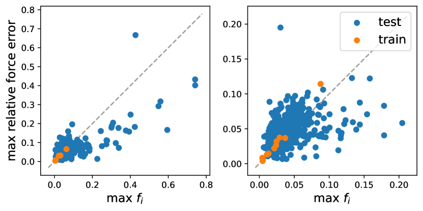
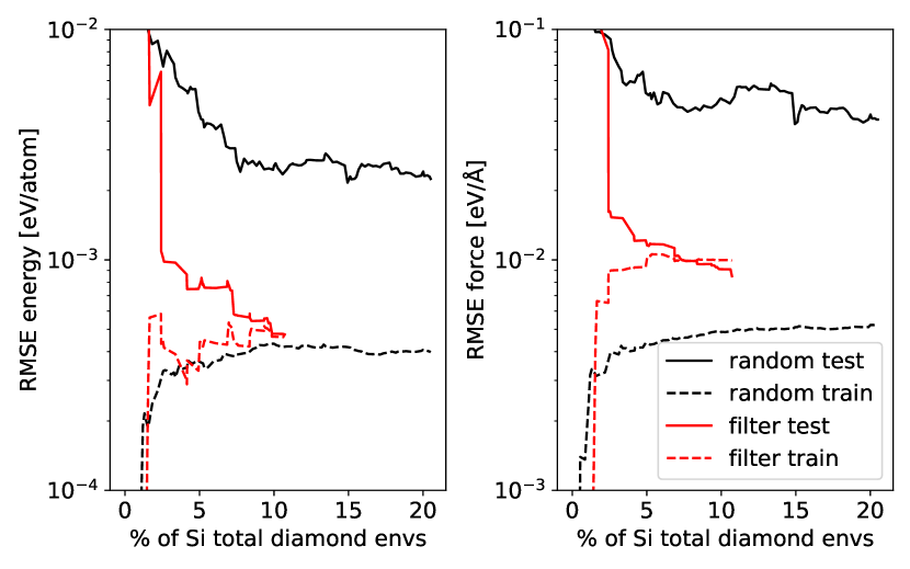
Figure 1: a) Maximum relative force error estimate $\max f_{i}$ versus error correlation plots for silicon diamond containing 4 and 10 training configurations. b) Learning rate comparison between filtering and random selection for silicon diamond.

Prior to training database reduction the ability of the relative force error estimate $f_{i}$ to predict relative force error is investigated. Fig. 1a compares the maximum relative force error in a configuration against the maximum of $f_{i}$ for two different training databases, containing 4 and 10 silicon diamond configurations respectively. The test configurations are the remaining configurations contained in the 489 silicon diamond configurations as part of the entire silicon database (totalling 16708 local environments). The regularising constant $\varepsilon$ was set to the mean force magnitude as predicted by the mean parameterisation. Both figures show good correlation between maximum relative force error and $\max\,f_{i}$, therefore making it a suitable criterion to be monitored during (H)AL strategies.

By leveraging the correlation of $f_{i}$ with true relative force error the existing silicon diamond database can be reduced by iteratively selecting configurations containing the largest relative force uncertainty as part of a greedy algorithms strategy. To demonstrate this a single configuration from the 489 silicon diamond configurations the silicon database was fitted. Next, $f_{i}$ was determined over the remaining configurations and the configuration containing the largest $\max\,f_{i}$ added to the training database. This process was repeated train and test error of this filtering procedure for silicon diamond is shown in Fig. 1b. It is benchmarked against performing random selection whereby, starting from the same initial configuration, test configurations were chosen at random from the pool of remaining . The result indicates that $f_{i}$ accurately detects configurations with large errors and manages to accelerate the learning rate significantly relative to random selection. Good generalisation between training and test errors is achieved by using around 5$\%$ of the total environment contained in the original silicon diamond database.

II.1.2 Si diamond: property convergence

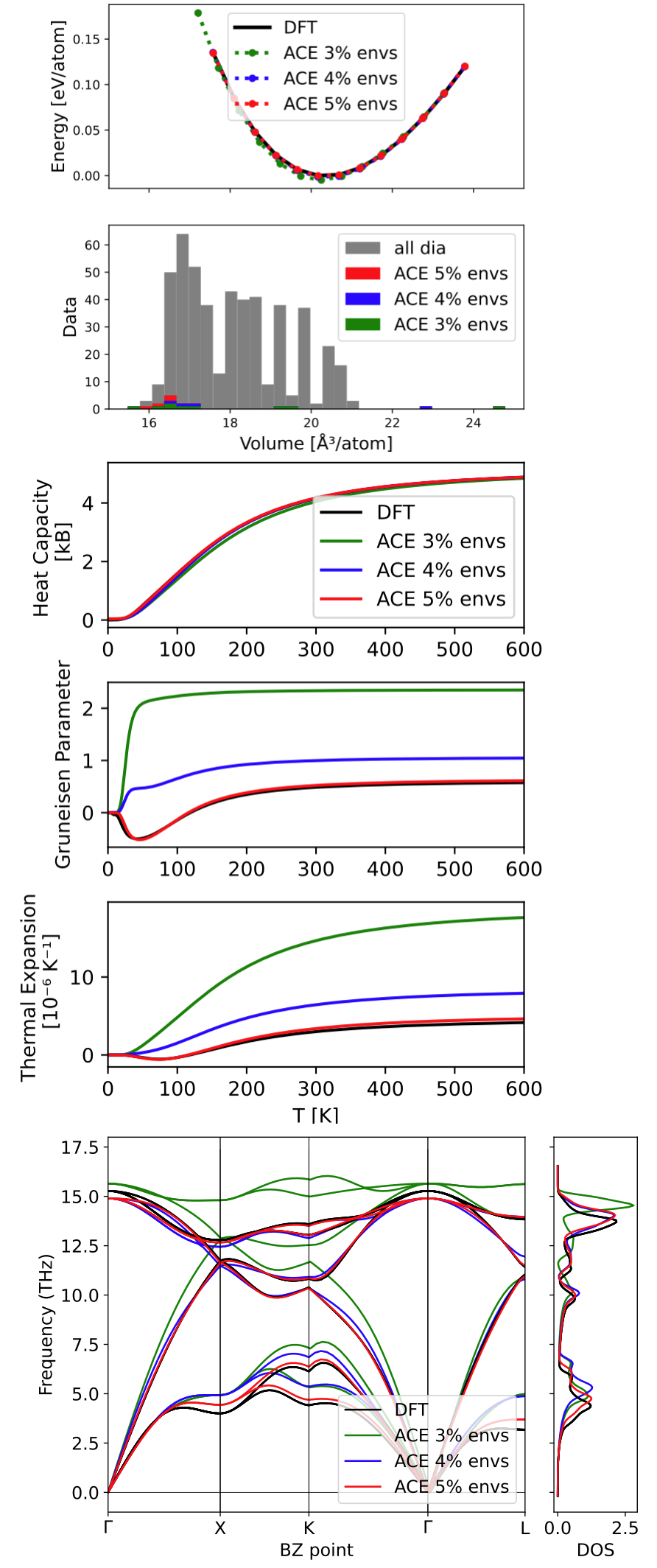
Figure 2: Property convergence for the energy volume (top), thermal properties (middle) and phonon spectrum (bottom) for filtering silicon diamond ACE models.

The significant acceleration of the learning rate shown in Fig. 1b shows that generalisation between train and test error is rapidly achieved, in turn suggesting that property convergence is accelerated too. This is investigated These properties elastic constants, energy volume curves, phonon spectrum and thermal properties for bulk silicon diamond.

Fig. 2 demonstrates that property convergence for the energy volume curves, phonon spectrum and thermal properties are rapidly achieved by fitting to a fraction of the original database. to 5$\%$ of the original database reaches sufficient accuracy to describe all properties with good accuracy with respect to the DFT reference. This is again confirmed by elastic constants as predicted by the respective models as shown in Table. 1. The convergence of the phonon spectrum in Fig. 2 is particularly noteworthy as relative errors on the order of a few percent on small forces $\sim$ 0.01 eV/$\mathrm{\SIUnitSymbolAngstrom}$ are .

	$B$	$c_{11}$	$c_{12}$	$c_{44}$
ACE 3% envs	98.2	188.1	53.3	79.7
ACE 4% envs	84.2	159.8	46.4	75.7
ACE 5% envs	82.5	148.7	49.3	73.7
DFT	82.6	147.2	50.3	73.1

Table 1: Convergence of the elastic moduli (GPa) of the filtered ACE models relative to the CASTEP DFT reference.

II.2 AlSi10

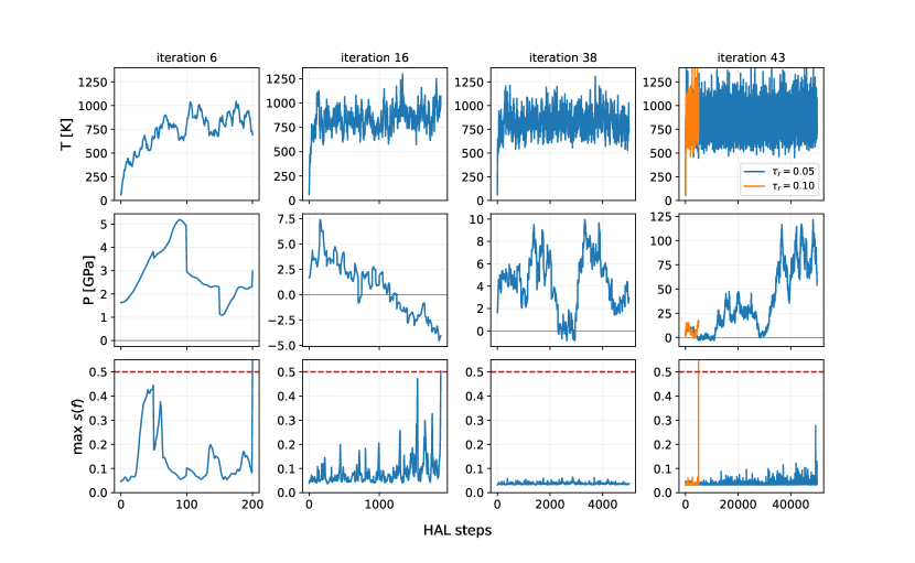
Figure 3: HAL dynamics for several iterations for the AlSi10 random alloy showing softmax normalised relative force error estimate $s(f)$, temperature and pressure. DFT calculations are triggered if the tolerance in red is reached. Pressure fluctuations are due to swap/volume MC steps on HAL potential energy surface $E_{\rm HAL}$.

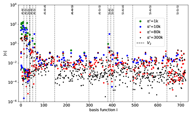
Figure 4: Coefficient magnitude $|\mathbf{c}_{i}|$ for the 723 basis functions grouped per correlation order and element interaction for various ARD tolerances $\alpha^{\prime}$. Large coefficients are assigned to pair interactions, partly captured by the auxiliary pair potential $V_{2}$, as most of the binding energy is contained in these interactions.

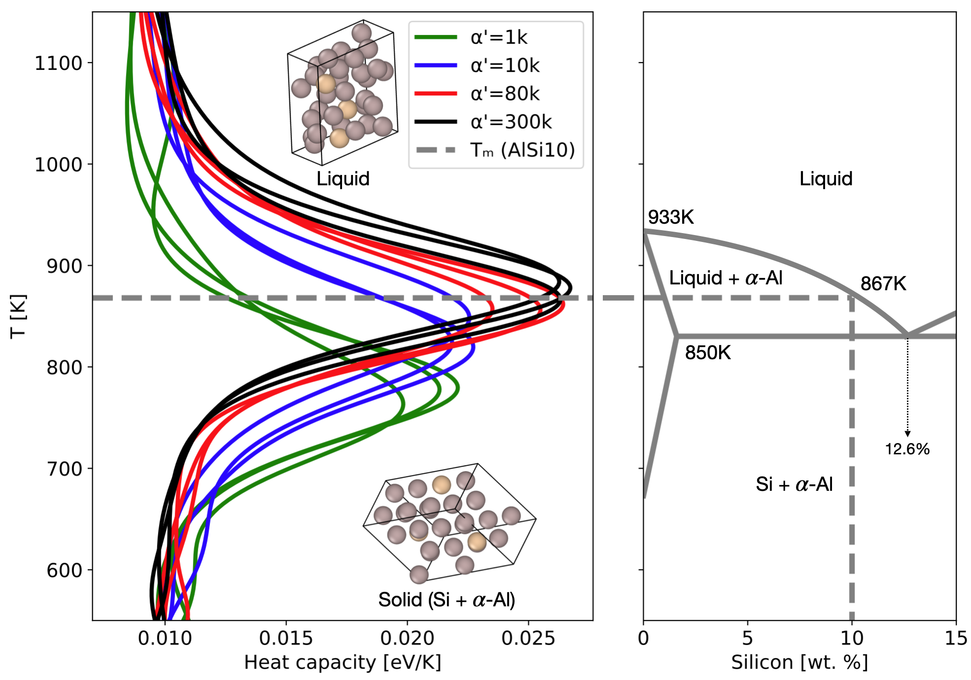
Figure 5: NS determined heat capacity for ARD fitted linear AlSi10 ACE models (left) and schematic phase diagram for AlSi10 [61] (right). Excellent agreement with the melting temperature is demonstrated for fits with large $\alpha^{\prime}$.

$\alpha^{\prime}$	$N_{\textrm{basis}}$	Performance	Fit	Training Error		Test Error
		($\mu$s/atom	(s)	E	F	E	F
		/core)		(meV/at)	(eV/$\mathrm{\SIUnitSymbolAngstrom}$)	(meV/at)	(eV/$\mathrm{\SIUnitSymbolAngstrom}$)
1$k$	38	62	2	7.693	0.135	8.006	0.147
10$k$	116	83	3	4.199	0.095	6.229	0.104
80$k$	295	85	17	2.401	0.080	5.131	0.089
300$k$	621	99	63	1.869	0.074	5.188	0.095

Table 2: Train/test error splits for HAL generated AlSi10 database for varying ARD tolerance $\alpha^{\prime}$. Larger ARD tolerance $\alpha^{\prime}$ includes more basis functions but increases performance and fitting time.

This section outlines the general HAL protocol for building training databases for alloys and demonstrates how an AlSi10 linear ACE model is built from scratch in an automated fashion. By using the relative force error estimate $f_{i}$ previously discussed as a stopping criterion to trigger ab initio evaluations it will be shown how an ACE model is created for AlSi10 using HAL. The HAL generated ACE model will be able to accurately model the liquid-solid phase transition and predict its melting temperature with excellent accuracy. The ACE models used in this section contained basis functions $\nu=2$ and polynomial degree 13 as well as an outer cutoff 5.5 $\mathrm{\SIUnitSymbolAngstrom}$. The ACE inner cutoff was set to 1.5 $\mathrm{\SIUnitSymbolAngstrom}$ during the HAL stage of collecting data and moved towards the closest interatomic distance once all training data had been generated. An auxiliary pair potential $V_{2}$ added to aid stability also added to the basis including functions up to polynomial degree 13 and an outer cutoff of 6.0 $\mathrm{\SIUnitSymbolAngstrom}$. The weights for the energy $w_{E}$, forces $w_{F}$ and virials $w_{V}$ were set to .

The HAL procedure of building ACE models for alloys starts by creating set of a random crystal structures manually, from which a random alloy and liquid alloy training database are built in an iterative fashion. Once sufficient data for both phases has been collected, the HAL solid and liquid databases are afterwards combined in order to create a model accurately both phases. The first step in the HAL protocol is the creation of a set of small initial random alloy database, which was formed of 32-atom FCC lattice configurations populated with 29 Al and 3 Si atoms, equivalent to 9.7 weight percent Si. This initial random alloy starting database contained 10 configurations with lattice constants ranging from 3.80 $\mathrm{\SIUnitSymbolAngstrom}$ to 4.04 $\mathrm{\SIUnitSymbolAngstrom}$ and was evaluated using CASTEP [62] DFT. The main parameters chosen are as follows: plane-wave cutoff 300 eV, kpoint spacing 0.04 $\mathrm{\SIUnitSymbolAngstrom}$^-1, 0.1 eV smearing, Pulay density mixing scheme and finite basis correction.

An adaptive biasing parameter $\tau_{\textrm{r}}$=0.05 was chosen (for explicit definition see Methods section) and the temperature set to $T_{\textrm{solid}}$=800K in order to build the random solid alloy database starting from the 10 initial structures previously described. Besides running biased dynamics, HAL performed cell volume adjusting (adding Gaussian noise to cell vectors) and element swapping Monte Carlo (MC) steps during the simulation on the HAL potential energy surface $E_{\rm HAL}$. These steps were accepted or rejected according to the Metropolis-Hastings algorithm [63].

During HAL dynamics the softmax normalised relative force estimate $s(f)$ is evaluated and a ground-truth evaluation triggered once a predefined tolerance of $s^{\textrm{tol}}$=0.5 is met. A total of 42 HAL configurations were sampled as the HAL dynamics at this stage was stable for 5000 steps The pressure $P$, temperature $T$ and $f_{i}$ are shown in Fig. 3 for four iterations with the first three being included in the training database, e.g. below or equal to iteration 42. The strong oscillations in the pressure $P$ are due to the volume and element swapping MC steps being accepted.

HAL trajectories were simulated using a Langevin thermostat targeting a temperature regime of $T_{\textrm{liquid}}$=3000K, and and a proportional control barostat targeting pressure level of 0.1 GPa. No volume or swap MC steps were performed.

After generating generating 46 liquid alloy configurations using HAL the dynamics stable for 5000 steps and

shown in Table 2. The test set was assembled by continuing HAL iterations for both the random alloy and liquid. Increasing $\alpha^{\prime}$ lowers the relevance criterion for the linear ACE basis functions in turn decreasing sparsity. A clear trade-off between sparsity and training error can be seen in Table 2 which also includes model evaluation performance and fitting times. Increasing $\alpha^{\prime}$ not only decreases training error but also test error up to $\alpha^{\prime}=300k$ for which the test error increases, a sign of overfitting. Due to the relatively small training database size remains low, around a minute or less using 8 threads on Intel(R) Xeon(R) Gold 5218 CPU @ 2.30GHz. Performance testing was done using LAMMPs and the PACE evaluator [64] on the exact same processor and show that all models are within 100 $\mu$s/atom/core per MD step.

Further analysis of the ARD fitted models was done by examining the absolute value of the coefficients $|\mathbf{c}_{i}|$. Basis functions below the predefined threshold are pruned away as can be seen in Fig. 4. Large coefficients are given to the pair interactions described by the auxiliary basis $V_{2}$ and two-body components of the ACE basis for all models, which is intuitive as most binding energy is stored in these pair interactions. Increasing $\alpha^{\prime}$ results in more (less relevant) basis functions being included with relatively smaller coefficients. For $\alpha^{\prime}=300k$ many of these low relevance coefficients of around $10^{-4}$ are included in the fit indicating a degree of overfitting - as confirmed by the test set error increase in Table 2.

Next the melting temperature for each of the previously ARD fitted AlSi10 ACE models is determined. This was done using Nested Sampling (NS) which approximates the partition function of an atomic system by exploring the potential energy surface over decreasing energy (or enthalpy) levels, in turn determining the cumulative density of states [65]. From the partition function any thermodynamic quantity can be derived such as the heat capacity. The heat capacity exhibits a signature peak for first-order phase transitions, which includes the liquid-solid transition occurring at the melting temperature. Extensive previous work has shown that NS is an accurate and reliable method for determining the melting temperature [66, 67]. As it explores the entirety of configurational space including gas, liquid and solid phases NS also serves as an excellent test for model robustness. This robustness is partly achieved by the addition of the auxiliary pair potential previously described as $V_{2}$ which is added in order to ensure close range repulsion between atoms.

Starting from the gas phase (initial cell volume of 500 $\mathrm{\SIUnitSymbolAngstrom}$³/atom) the walkers explored the potential energy surface by iteratively cloning and decorrelating walkers at decreasing enthalpy levels, passing through the liquid phase and ending up at the ground structure. The decorrelation was done by running MD for 6 timesteps using a 0.1 fs timestep and a total of 1024 MC steps by changing the cell volume, shearing/stretching the cell and swapping atoms (ratio 6:6:6:6) were performed. The NS cell pressure was set to 0.1 GPa and the minimum aspect ratio of the cell set to 0.85. By summing the enthalpies from the NS simulation the constant pressure partition function is determined from which the heat capacity can be derived through postprocessing. Three independent runs for each of the ARD models fitted to the AlSi10 HAL database were performed. shown in Fig. 5. All models predicted the expected FCC ground structure, but a difference in predicted melting temperature for varying $\alpha^{\prime}$ can be seen. Only the $\alpha^{\prime}=300k$ and $\alpha^{\prime}=80k$ models accurately the melting temperature of 867K as predicted by Thermo-Calc with the TCAL4 database [68]. Table 2

II.3 Polyethylene glycol (PEG)

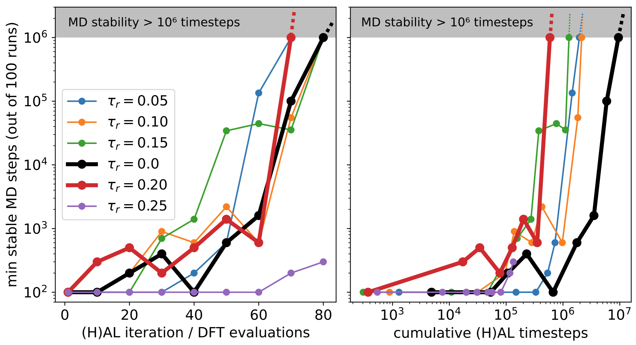
Figure 6: HAL vs AL benchmark comparing MD stability for 1 million MD steps over 100 seeds. Turning on biasing (non-zero $\tau_{\textrm{r}}$) creates ACE models achieving stable 100 million MD timestep faster than standard AL by up to an order of magnitude.

This section presents the application of HAL to build databases for polymers. Polyethylene glycol (PEG) has the formula H[OCH₂CH₂]_nOH, where $n$ is the number of monomer units [69]. From a modelling perspective these polymers are challenging to simulate in vacuum as they form configurations ranging from tightly coiled up to fully stretched out structures. Due to the OH group at the end the polymer can also exhibit hydrogen bonding, which further complicates its description. These hydrogen bonds typically correspond to low energy configurations and are frequently formed and broken during long MD simulations. This section first presents a benchmark of HAL against AL followed by a demonstration HAL finding configurations exhibiting large errors. Finally, the potential fitted to small polymer units in vacuum is used to predict the density of a long PEG($n$=200) polymer in bulk with excellent accuracy relative to experiment. All DFT reference calculations in this section are carried out with the ORCA code [70] using the $\omega$B97X DFT exchange correlation functional [71] and 6-31G(d) basis set.

II.3.1 PEG($n$=2): HAL vs AL

In order to test whether HAL accelerates training database assembly relative to standard AL, a benchmark test was performed. An initial database containing 20 PEG($n$=2) polymers was created by running 500 K NVT molecular dynamics simulation using the general purpose ANI-2x forcefield [11] sampling every 7 ps. This database was fitted using an ACE basis containing basis functions up to correlation order $\nu$=3 and polynomial degree 10 with an outer cutoff 4.5 $\mathrm{\SIUnitSymbolAngstrom}$ and inner cutoff 0.5 $\mathrm{\SIUnitSymbolAngstrom}$. The auxiliary pair potential basis up to polynomial degree 10 and outer cutoff 5.5 $\mathrm{\SIUnitSymbolAngstrom}$ and did not have an inner cutoff. The weights for the energy $w_{E}$, forces $w_{F}$ were set to 15.0 and 1.0 and remain constant throughout this seciton on PEG. AL (non-biasing, or $\tau$=0.0) and HAL simulations with varying biasing strengths $\tau_{\textrm{r}}$ were performed using a timestep of 0.5 fs at 500K. Configurations were evaluated using ORCA DFT once $s^{\textrm{tol}}$=0.5 was reached.

The linear ACE models generated during the AL/HAL simulations were saved and subsequently used in a regular MD stability test and ran for 1 million MD steps at 500 K using a 1 fs timestep for 100 separate runs. A MD simulation was deemed stable if the CC and CO bonds along the chain where within 1.0-2.0$\mathrm{\SIUnitSymbolAngstrom}$ and the CH and OH bonds within 0.8-2.0$\mathrm{\SIUnitSymbolAngstrom}$ during the simulation. The minimum number of stable MD timesteps out of the 100 different simulations is shown in Fig.6 and demonstrates that up to $\tau_{\textrm{r}}$=0.20 a total of 80 (H)AL iterations are required in order to achieve a minimum MD stability of 1 million steps. The large biasing strength of $\tau_{\textrm{r}}$=0.25 results in unstable MD dynamics as too strong biasing causes the generation of exceedingly high energy configuration far away from the desired potential energy surface to be included in the training database. Fitting to these configurations leads to a poorly performing model as many unphysical configurations enter the training database resulting.

The HAL run using a biasing strength of $\tau_{\textrm{r}}$=0.20, achieves minimum 1 million step MD stability after an order of magnitude fewer exploratory MD timesteps compared to standard AL.

II.3.2 PEG($n$=4): rare events

Using PEG($n$=4) polymers this section will investigate the ability of HAL to generate and detect configurations with large errors. First a training database was built using the general purpose ANI-2x forcefield [11] at 500K and 800K using a timestep of 1 fs. Configurations were sampled every 7000 timesteps (7 ps), and used to assemble 500K and 800K databases. The 500K database was divided into 750 train configurations and 250 test configurations. The 800K training and test databases both contained 250 configurations. The linear ACE model was extended to include basis functions up to 12 for both the ACE and pair potential, while keeping the cutoffs and correlation order the same ($\nu$=3) too compared to the previous section on PEG($n$=2).

Using the 500K MD sampled training database HAL was started using $\tau_{\textrm{r}}$=0.10 and a timestep of 0.5 fs. The stopping criterion $s^{\textrm{tol}}$ set to 0.5. A total of 200 HAL configurations were generated and formed a HAL database used for both a train and test set. Using the previously described basis three models were created fitted to: 500K, 500K+800K and a 500K+HAL. Energy scatter plots for these three models are shown in Fig. 7 demonstrating that the errors on the HAL-found configurations are large for both the 500K and 500K+800K fits, despite the fact that the these HAL-found configurations are also low in energy! Only by including the HAL configurations in the training database can the errors on these configurations be reduced as shown in Table. 3. Inspection of the HAL generated structures exposes a shared characteristic: most of them contain (double) hydrogen bonding across the polymer an example of which is shown in Fig. 7. Such hydrogen-bond formation is a rare event in this system, because only the two ends of the molecule are capable of hydrogen bonding. It is difficult to find these configurations using regular MD (even when using elevated temperatures), whereas HAL finds them easily.

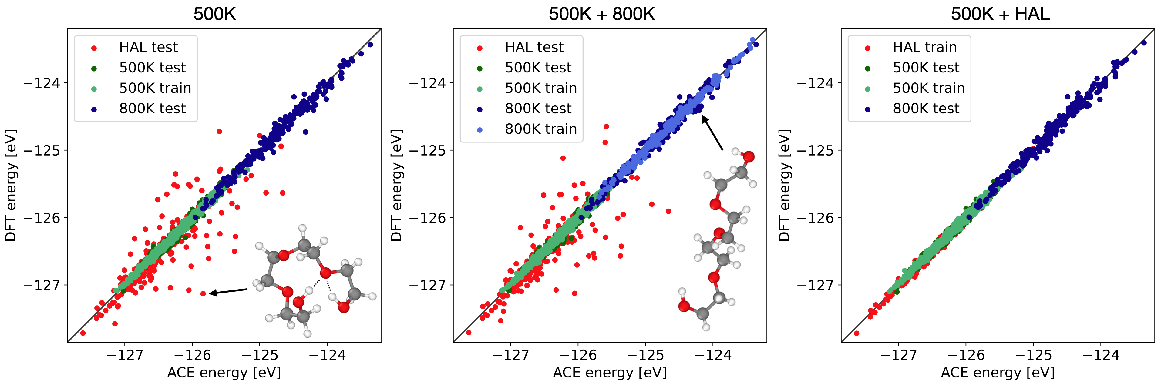
Figure 7: Energy scatter plots for the 500K (left), 500K+800K (middle) and 500K+HAL (right) ACE models. HAL configuration mostly exhibit (double) hydrogen bonding, or rare events, not contained in the MD 500K/800K decorrelated samples.

	No.	500K		500K+800K		500K+HAL
	configs	E	F	E	F	E	F
500K train	750	30.2	58.3	32.9	60.8	32.4	59.6
500K test	250	49.2	79.3	48.8	76.7	41.6	71.0
800K train	250	-	-	40.0	76.4	-	-
800K test	250	72.7	187.2	67.6	107.7	67.9	102.6
HAL	200	310.9∗	427.2∗	311.9∗	404.6∗	47.8†	63.4†

Table 3: Train and test errors for energies (E) in meV and forces (F) in meV/$\mathrm{\SIUnitSymbolAngstrom}$ for the 500K, 500K+800K and 500K+HAL databases using ACE. ^† is train error. ^∗ is test error.

II.3.3 PEG($n$=200): bulk density

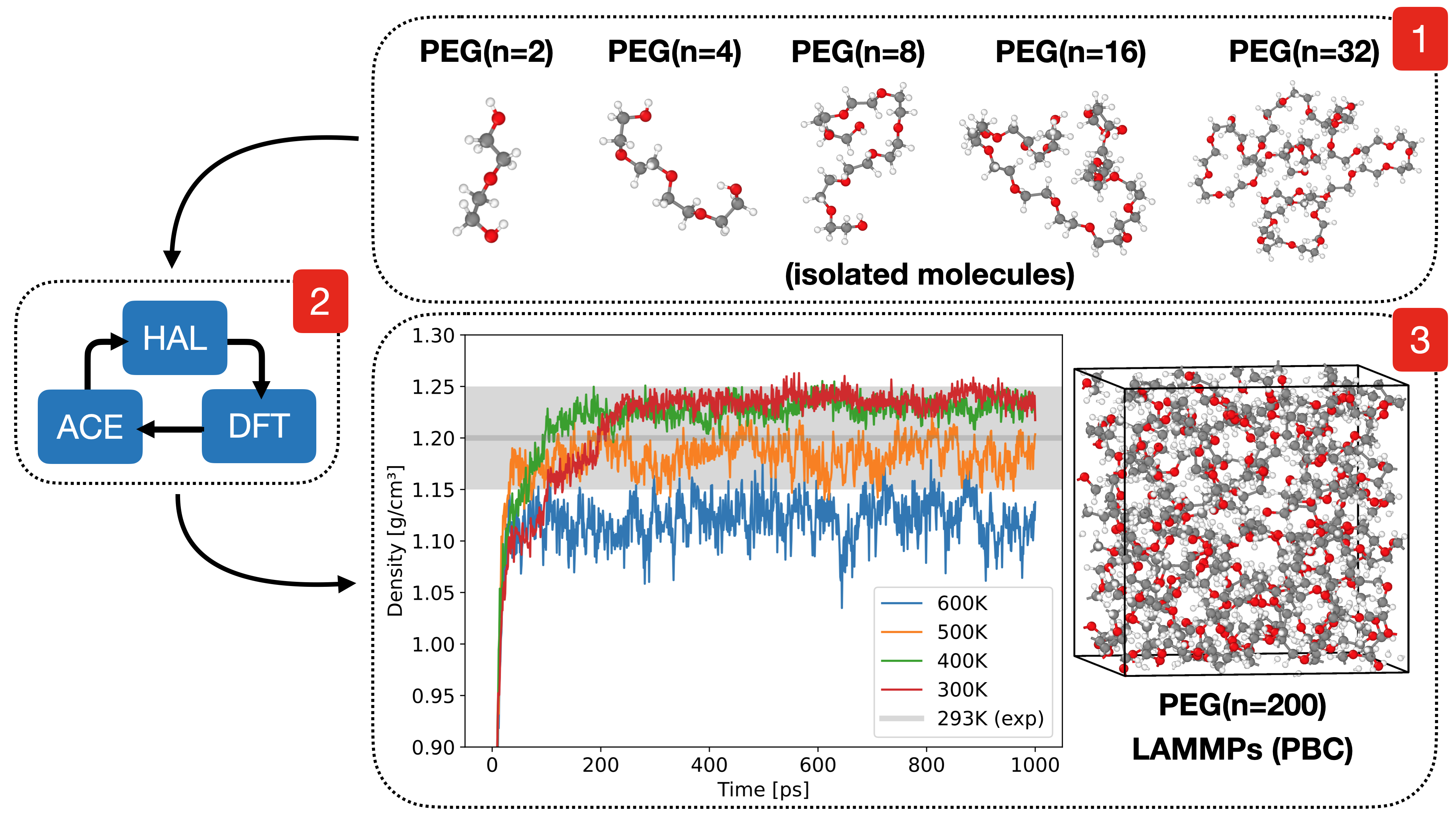
Figure 8: HAL protocol for building linear ACE PEG model accurately determining PEG($n$=200) density within experimental accuracy of 1.2 g/cm³ at 297K (shaded area) [72]. Training database only included small polymers ranging from $n$=2 to $n$=32 in isolation.

As a final investigation the density of a PEG($n$=200) polymer containing 1400 atoms is determined using an ACE model fitted to a HAL generated PEG training database containing polymer sizes ranging from $n$=2 to $n$=32 monomer units. This database contained configurations from the previous PEG sections and extended using configurations sized $n=8$, $n=16$ and $n=32$. The training database included standard ANI MD sampled configurations at 500K including 1000 PEG(n=$4$) configurations (from the previous section), as well as 50 PEG($n$=2), 100 PEG($n$=8), 100 PEG($n$=16) and 18 PEG($n$=32) configurations. Starting from this data HAL was used to generate an extra 64 PEG($n$=16) and 91 PEG($n$=32) HAL configurations until dynamics was deemed stable. The linear ACE basis used for the regression task was identical to the ACE in the previous section on PEG($n$=4), and any force components with greater than 20 eV/$\mathrm{\SIUnitSymbolAngstrom}$ were excluded from the fit.

Using the ACE model a PEG($n$=200) polymer was simulated in LAMMPS [73] with the PACE evaluator pair style with periodic boundary conditions. Since the training database only contained small polymers segments in vacuum this periodic simulation demonstrates a large degree of extrapolation to configurations far away from the training database. Furthermore, the DFT code used to evaluate the training energies and forces does not support periodic boundary conditions making DFT simulation of the 1400 atom PEG($n$=200) simulation box not just computationally infeasible, but practically impossible in this case.

The resulting linear ACE model was timed at 220 $\mu$s/atom/core per MD step. LAMMPs NPT simulations were performed at 1 bar using a 1 fs timestep at 300K, 400K, 500K and 600K. The recorded density as a function of simulation time is plotted in Fig. 8. Using the last 500 ps from the 300K simulation the density was determined to be 1.238 g/cm³. This value is around 3$\%$ higher than the experimental value of 1.2 g/cm³ [72].

III Methods

III.1 Hyperactive Learning (HAL)

The HAL potential energy $E_{\rm HAL}$ as defined in Eq. (1) biases MD simulations during the exploration step in AL towards uncertainty by shifting the potential energy surface and assigning lower energies to configurations with high uncertainty. We have shown that when $\sigma$ is the standard deviation of the posterior-predictive uncertainty of energy, it can be computationally cheaply approximated by a Monte-Carlo estimate $\tilde{\sigma}$; see (5). Likewise, the derivative of $\tilde{\sigma}$ can be computed as

$$\nabla\tilde{\sigma}=\frac{\nabla\tilde{\sigma}^{2}}{2\tilde{\sigma}}$$ (9)

where

$$\begin{split}\nabla\tilde{\sigma}^{2}&=\frac{2}{K}\sum_{k=1}^{K}\left(E^{k}-\bar{E}\right)\left(\nabla E^{k}-\nabla\bar{E}\right)\\ &=\frac{2}{K}\sum_{k=1}^{K}\left(E^{k}-\bar{E}\right)\left(\bar{F}-F^{k}\right)\end{split}$$ (10)

and $F^{k}=-\nabla E^{k}$, $\bar{F}=-\nabla\bar{E}$. These predictions are obtained by ensemble parameterisations $\{\mathbf{c}_{k}\}_{k=1}^{K}$, while $\bar{\mathbf{c}}$ is the analytic mean of the posterior distribution as specified in (22). The sum over $K$ is over the ensemble or committee of models, which in this work was chosen to be linear (ACE) models. Other architectures such as neural networks ensembles may be considered in future work. This quantity in essence is a computationally cheap method of determining the gradient towards (total) energy uncertainty and may be interpreted as a conservative biasing force,

$$F^{\tilde{\sigma}}:=\nabla\tilde{\sigma}.$$ (11)

HAL dynamics adds this biasing force to MD in order to accelerate the generation of configurations with high uncertainty, which sets HAL apart from AL. Setting $\tau$=0 recovers standard MD dynamics, and in this sense, HAL generalizes AL. Interestingly, previous work employed a biasing force using a neural network interatomic potential [74] but biased away from uncertainty in order to stabilise the MD dynamics.

The biasing strength $\tau$ can either be set as a constant or adapted during the HAL simulation. Controlling the biasing strength is important as too strong biasing can quickly lead to unphysical configurations, whereas low biasing generates valuable configurations at a slow rate. The adaptive biasing works by first setting $\tau_{\textrm{r}}$ and performing a burn-in period to record the magnitudes (or, norms) of $F^{\tilde{\sigma}}$ and $\bar{F}$. Typically, the burn-in period is set to the latest 100 timesteps $\delta t$. The biasing strength $\tau$ is then determined by satisfying

$$\tau_{\textrm{r}}=\frac{\tau\sum_{m=1}^{100}\|\bar{F}(t-m\delta t)\|}{\sum_{m=1}^{100}\|F^{\tilde{\sigma}}(t-m\delta t)\|}.$$ (12)

The new parameter $\tau_{\textrm{r}}$ is generally set between 0.05 and 0.25. It can be understood as the approximate relative average strength of the biasing force in comparison to the average force of the fitted model. Using this adaptive biasing term aids usability and tunes the biasing strength to ensure that HAL gently drives MD towards high uncertainty. The value may loosely be interpreted as the relative magnitude of the biasing force compared to the true gradient of the potential energy surface. Larger $\tau_{\textrm{r}}$ increases the biasing strength and rate at which configurations with high uncertainty are generated. In order to sample configurations at desired pressures and temperatures a proportional control barostat was added as well as a Langevin thermostat.

III.2 Atomic Cluster Expansion (ACE)

The ACE model decomposes the total energy $E$ of a configuration $R$ as a sum of parameterised atomic energies,

$$E(\mathbf{c};R)=\sum_{i\in R}E_{i}(\mathbf{c};R).$$ (13)

The atomic energies $E_{i}$ are then parameterised by a linear model, $E_{i}={\bf c}\cdot{\bf B}_{i}$, where ${\bf B}_{i}$ denotes the ACE basis. The present work employs a particularly simple variant, which we review briefly: Given relative atomic positions $\bm{r}_{ji}=\bm{r}_{j}-\bm{r}_{i}$ and associated chemical elements one evaluates a one-particle basis

$$\phi_{znlm}(\bm{r}_{ji},z_{j})=\delta_{zz_{j}}R_{n}(r_{ji})Y_{lm}(\hat{\bm{r}}_{ji}),$$ (14)

followed by a pooling operation resulting in features

$$A_{iznml}=\sum_{j}\phi_{znlm}(\bm{r}_{ji},z_{j}),$$ (15)

that are denoted the atomic basis in the context of the ACE model. Taking a $\nu$ order (tensor) product results in many-body correlation functions incorporating ($\nu$+1) body-order interactions,

$$\mathbf{A}_{i\mathbf{znlm}}=\prod^{\nu}_{t=1}A_{iz_{t}n_{t}l_{t}m_{t}}.$$ (16)

The $\mathbf{A}$-basis is a complete basis of permutation-invariant functions but does not incorporate rotation or reflection symmetry. An isometry invariant basis $\mathbf{B}$ is constructed by averaging over rotations and reflections. Representation theory of the orthogonal group $O(3)$ shows that this can be expressed as a sparse linear operation and results in

$$\mathbf{B}_{i}=\mathbf{C}\mathbf{A}_{i},$$ (17)

where $\mathbf{C}$ contains generalised Clebsch-Gordan coefficients; we refer to [24, 25] for further details.

A major benefit of the linear ACE model is that the computational cost of evaluating a site energy $E_{i}$ scales only linearly with the number of neighbouring atoms, as well as with the body order $\nu+1$.

III.3 (Bayesian) Linear Regression

The parameters of linear ACE models are fitted by solving a linear regression problem. The associated squared loss function $L(\mathbf{c})$ to be minimised over configurations $R$ in training set $\bm{R}$ with corresponding (DFT) observations for energy $\mathscr{E}_{R}$, forces $\mathscr{F}_{R}$ is

$$\begin{split}L(\mathbf{c})=\sum_{R\in\bm{R}}(w_{E}|E(\mathbf{c};R)-\mathscr{E}_{R}|^{2}\\ +w_{F}|F(\mathbf{c};R)-\mathscr{F}_{R}|^{2})\end{split}$$ (18)

where $w_{E}$ and $w_{F}$ are weights specifying the relative importance of the DFT observations. When fitting materials a third term is added $w_{V}|V(\mathbf{c};R)-\mathcal{V}_{R}|^{2}$ referring to the virial stress components of the configuration $R$. This minimisation problem can be recast in the generic form

$$\underset{\mathbf{c}}{\arg\min}\,\,\|\mathbf{y}-\mathbf{\Psi}\mathbf{c}\|^{2}+\eta\|\mathbf{c}\|^{2},$$ (19)

where is the design matrix and collects the observations to which the parameters are fitted. Here, we also added a Tychonov regularisation with regularisation parameter $\eta>0$ which is commonly determined through a model selection criterion such as cross-validation.

This linear regression model can be cast in a Bayesian framework by specifying a prior distribution $p({\bf c})$ over the regression parameters, and an (additive) probabilistic

$$\mathbf{y}=\mathbf{\Psi}\mathbf{c}+\bm{\epsilon},$$ (20)

noise model gives rise to the likelihood function

$$\begin{split}p(\mathbf{y}|\mathbf{R},\mathbf{c},\lambda)=\left(\frac{\lambda}{2\pi}\right)^{N_{\textrm{obs}}/2}\exp\left\{-\frac{\lambda}{2}\|\mathbf{y}-\mathbf{\Psi}\mathbf{c}\|^{2}\right\}\end{split}$$ (21)

By restricting ourselves to a Gaussian error model, and assuming the prior to be Gaussian as well, i.e., $p({\bf c})=\mathcal{N}({\bf c}|{\bf 0},{\bf\Sigma}_{0})$, it is ensured that the posterior distribution, $\pi({\bf c})=p(\mathbf{c}|{\bf R},\mathbf{y},\lambda)$, is Gaussian with closed form expressions for both the distribution mean $\bar{\bf c}$ and variance ${\bf\Sigma}$,

$$\begin{split}\bar{\mathbf{c}}&=\lambda\bm{\Sigma}\mathbf{\Psi}^{T}\mathbf{y}\\ \bm{\Sigma}^{-1}&={\bf\Sigma}_{0}^{-1}+\lambda\mathbf{\Psi}^{T}\mathbf{\Psi}.\end{split}$$ (22)

In the context of this work, having closed form expressions for both these quantities is desirable as it (i) allows for conceptual easy and fast generation of independent samples $\{{\bf c}^{k}\}_{k=1}^{K}$ from the posterior distribution, and (ii) allows for a parametrisation of the fitted model with the exact mean, $\bar{\bf c}$, of the posterior distribution.

In what follows we briefly describe two Bayesian regression techniques, Bayesian Ridge Regression (BRR), which we use to produce Bayesian fits during the HAL data generation phase, and the Automatic Relevance Determination (ARD), which we typically use to obtain a final model fit after the data generation is complete.

III.4 Bayesian Ridge Regression (BRR)

In Bayesian Ridge Regression the covariance of the prior is assumed to be isotropic, i.e.,

$$p(\mathbf{c}|\alpha)=\mathcal{N}(\mathbf{c}|{\bf 0},\alpha^{-1}\mathbf{I}),$$ (23)

for some hyper-parameter $\alpha>0$, the precision of the prior distribution.

Under this choice of prior, the logarithm of the posterior distribution takes the form

$$\ln\pi({\bf c})=-\frac{\lambda}{2}\|\mathbf{y}-\mathbf{\Psi}\mathbf{c}\|^{2}-\frac{\alpha}{2}\|\mathbf{c}\|^{2}+\textrm{C},$$ (24)

where $C$ is some constant. Thus, maximising the (log-)posterior for this choice of prior, is equivalent to solving the regularised least square problem Eq. 24 with ridge penalty $\eta=\alpha/\lambda$. This shows that the prior naturally gives rise to a regularised solution, keeping coefficient parameters small.

The determination of the hyper-parameters $\alpha$ and $\lambda$ in BRR is achieved by optimising the marginal log likelihood also known as evidence maximisation [75]. One first defines the evidence function as

$$p(\mathbf{y}|\alpha,\lambda)=\int p(\mathbf{y}|\mathbf{c},\lambda)p(\mathbf{c}|\alpha)d\mathbf{c}$$ (25)

which marginalises out the coefficients $\mathbf{c}$ and describes the likelihood of observing the data given the hyperparameters $\alpha$ and $\lambda$. Using the previously defined definitions the evidence function can be expressed as

$$\begin{split}p(\mathbf{y}|\alpha,\lambda)=\left(\frac{\lambda}{2\pi}\right)^{N_{\textrm{obs}}/2}\left(\frac{\alpha}{2\pi}\right)^{N_{\textrm{basis}}/2}\\ \int\exp\left\{-\frac{\lambda}{2}\|\mathbf{y}-\mathbf{\Psi}\mathbf{c}\|^{2}-\frac{\alpha}{2}\|\mathbf{c}\|^{2}\right\}\end{split}$$ (26)

where $N_{\textrm{basis}}$ is the dimensionality of $\mathbf{c}$. Completing the square in the exponent and taking the log gives rise to the marginal log likelihood

$$\begin{split}\ln p(\mathbf{y}|\alpha,\lambda)=\frac{N_{\textrm{basis}}}{2}\ln\alpha+\frac{N_{\textrm{obs}}}{2}\ln\lambda\\ -\frac{\lambda}{2}\|\mathbf{y}-\mathbf{\Psi}\mathbf{c}\|^{2}-\frac{\alpha}{2}\|\mathbf{c}\|^{2}+\\ \frac{1}{2}\ln\|\bm{\Sigma}\|-\frac{N}{2}\ln(2\pi)\end{split}$$ (27)

which can be maximised with respect to $\alpha$ and $\lambda$ in order maximise the marginal likelihood and obtain the statistically most probably likely solution given the basis and data.

III.5 Automatic Relevance Determination (ARD)

Automatic Relevance Determination (ARD) modifies BRR by relaxing the isotropy of the prior and assigning a hyperparameter $\alpha_{i}$ to independently regularise each coefficient $c_{i}$. The corresponding prior is given by

$$\begin{split}p(\mathbf{c}|{\bm{\alpha}})&=\mathcal{N}(\mathbf{c}|{\bf 0,}\mathcal{A}^{-1})\\ \mathcal{A}&={\rm diag}(\alpha_{1},...,\alpha_{N_{\textrm{basis}}}).\end{split}$$ (28)

This prior determines the relevance of each parameter $c_{i}$, or basis function, which effectively results in a feature selection. Basis functions are ranked based on their relevance and are pruned if determined irrelevant, in turn producing a sparse solution. In practice, sparse models obtained through ARD often yield better generalisation than BRR. Using ARD requires the specification of a threshold parameter $\alpha^{\prime}$ setting the minimum relevance of basis functions included in the fit. Adjusting this parameter controls the balance between accuracy and sparsity of the model.

III.6 Posterior Predictive Distribution

A key property of the Bayesian approach is that it provides a way to quantify uncertainty in terms of the posterior-predictive distribution, which accounts both for parameter uncertainty as given by the posterior distribution as well as uncertainty due to observation error.

IV Data Availability

The data will be made available at time of publication.

V Code Availability

The HAL code will be made available at time of publication.

VI Acknowledgements

GC and CvdO acknowledge the support of UKCP grant number EP/K014560/1. CvdO would like to acknowledge the support of EPSRC (Project Reference: 1971218) and Dassault Systèmes UK. CO acknowledges support of the NSERC Discovery Grant (IDGR019381) and the NFRF Exploration Grant GR022937.

VII Author Contributions

CvdO developed efficient uncertainties for ACE models. MS conceived the idea of uncertainty-biasing of AL exploration. CvdO led the implementation of the HAL framework. DK helped generate data. CvdO wrote the first version of the manuscript. All authors discussed the theory and results and edited the manuscript.

VIII Competing Interests

The authors declare no competing interests.

References

- [1] Volker L. Deringer, Miguel A. Caro, and Gábor Csányi. Machine learning interatomic potentials as emerging tools for materials science. Advanced Materials, 31(46):1902765, 2019.
- [2] Volker L. Deringer, Albert P. Bartók, Noam Bernstein, David M. Wilkins, Michele Ceriotti, and Gábor Csányi. Gaussian process regression for materials and molecules. Chemical Reviews, 121(16):10073–10141, 08 2021.
- [3] John A. Keith, Valentin Vassilev-Galindo, Bingqing Cheng, Stefan Chmiela, Michael Gastegger, Klaus-Robert Müller, and Alexandre Tkatchenko. Combining machine learning and computational chemistry for predictive insights into chemical systems. Chemical Reviews, 121(16):9816–9872, 08 2021.
- [4] A.P. Thompson, L.P. Swiler, C.R. Trott, S.M. Foiles, and G.J. Tucker. Spectral neighbor analysis method for automated generation of quantum-accurate interatomic potentials. Journal of Computational Physics, 285:316–330, 2015.
- [5] Han Wang, Linfeng Zhang, Jiequn Han, and Weinan E. Deepmd-kit: A deep learning package for many-body potential energy representation and molecular dynamics. Computer Physics Communications, 228:178–184, 2018.
- [6] Ivan S Novikov, Konstantin Gubaev, Evgeny V Podryabinkin, and Alexander V Shapeev. The MLIP package: moment tensor potentials with MPI and active learning. Mach. Learn.: Sci. Technol., 2(2):025002, December 2020.
- [7] Gabriele C. Sosso, Volker L. Deringer, Stephen R. Elliott, and Gábor Csányi. Understanding the thermal properties of amorphous solids using machine-learning-based interatomic potentials. Molecular Simulation, 44(11):866–880, 2018.
- [8] Volker L. Deringer, Noam Bernstein, Gábor Csányi, Chiheb Ben Mahmoud, Michele Ceriotti, Mark Wilson, David A. Drabold, and Stephen R. Elliott. Origins of structural and electronic transitions in disordered silicon. Nature, 589(7840):59–64, 2021.
- [9] Venkat Kapil, Christoph Schran, Andrea Zen, Ji Chen, Chris J. Pickard, and Angelos Michaelides. The first-principles phase diagram of monolayer nanoconfined water. Nature, 609(7927):512–516, 2022.
- [10] Jörg Behler and Michele Parrinello. Generalized neural-network representation of high-dimensional potential-energy surfaces. Phys. Rev. Lett., 98:146401, Apr 2007.
- [11] Christian Devereux, Justin S. Smith, Kate K. Huddleston, Kipton Barros, Roman Zubatyuk, Olexandr Isayev, and Adrian E. Roitberg. Extending the applicability of the ani deep learning molecular potential to sulfur and halogens. Journal of Chemical Theory and Computation, 16(7):4192–4202, 2020. PMID: 32543858.
- [12] J. S. Smith, O. Isayev, and A. E. Roitberg. ANI-1: an extensible neural network potential with DFT accuracy at force field computational cost. Chemical Science, 8(4):3192–3203, 2017.
- [13] Han Wang, Linfeng Zhang, Jiequn Han, and Weinan E. DeePMD-kit: A deep learning package for many-body potential energy representation and molecular dynamics. Computer Physics Communications, 228:178–184, 2018.
- [14] Albert P Bartók and Gábor Csányi. Gaussian approximation potentials: A brief tutorial introduction. International Journal of Quantum Chemistry, 115(16):1051–1057, 2015.
- [15] Albert P. Bartók, Sandip De, Carl Poelking, Noam Bernstein, James R. Kermode, Gábor Csányi, and Michele Ceriotti. Machine learning unifies the modeling of materials and molecules. Science Advances, 3(12):1–9, 2017.
- [16] Anders S. Christensen, Lars A. Bratholm, Felix A. Faber, and O. Anatole Von Lilienfeld. FCHL revisited: Faster and more accurate quantum machine learning. Journal of Chemical Physics, 152(4), 2020.
- [17] Stefan Chmiela, Huziel E. Sauceda, Igor Poltavsky, Klaus Robert Müller, and Alexandre Tkatchenko. sGDML: Constructing accurate and data efficient molecular force fields using machine learning. Computer Physics Communications, 240:38–45, 2019.
- [18] Bastiaan J. Braams and Joel M. Bowman. Permutationally invariant potential energy surfaces in high dimensionality. International Reviews in Physical Chemistry, 28(4):577–606, 2009.
- [19] Cas van der Oord, Geneviève Dusson, Gábor Csányi, and Christoph Ortner. Regularised atomic body-ordered permutation-invariant polynomials for the construction of interatomic potentials. Machine Learning: Science and Technology, 1(1):015004, 2020.
- [20] Alice E A Allen, Geneviève Dusson, Christoph Ortner, and Gábor Csányi. Atomic permutationally invariant polynomials for fitting molecular force fields. Machine Learning: Science and Technology, 2(2):025017, 2021.
- [21] Aidan P Thompson, Laura P Swiler, Christian R Trott, Stephen M Foiles, and Garritt J Tucker. Spectral neighbor analysis method for automated generation of quantum-accurate interatomic potentials. Journal of Computational Physics, 285:316–330, 2015.
- [22] Albert P. Bartók, Mike C. Payne, Risi Kondor, and Gábor Csányi. Gaussian approximation potentials: The accuracy of quantum mechanics, without the electrons. Phys. Rev. Lett., 104:136403, Apr 2010.
- [23] Alexander V. Shapeev. Moment tensor potentials: A class of systematically improvable interatomic potentials. Multiscale Modeling & Simulation, 14(3):1153–1173, 2016.
- [24] Ralf Drautz. Atomic cluster expansion for accurate and transferable interatomic potentials. Physical Review B, 99(1):014104, 2019.
- [25] Geneviève Dusson, Markus Bachmayr, Gábor Csányi, Ralf Drautz, Simon Etter, Cas van der Oord, and Christoph Ortner. Atomic cluster expansion: Completeness, efficiency and stability. Journal of Computational Physics, 454:110946, 2022.
- [26] Dávid Péter Kovács, Cas van der Oord, Jiri Kucera, Alice EA Allen, Daniel J Cole, Christoph Ortner, and Gábor Csányi. Linear atomic cluster expansion force fields for organic molecules: beyond rmse. Journal of chemical theory and computation, 17(12):7696–7711, 2021.
- [27] Kristof T. Schütt, Farhad Arbabzadah, Stefan Chmiela, Klaus R. Müller, and Alexandre Tkatchenko. Quantum-chemical insights from deep tensor neural networks. Nature Communications, 8:6–13, 2017.
- [28] Brandon Anderson, Truong Son Hy, and Risi Kondor. Cormorant: Covariant molecular neural networks. Advances in Neural Information Processing Systems, 32(NeurIPS), 2019.
- [29] Oliver T. Unke and Markus Meuwly. PhysNet: A Neural Network for Predicting Energies, Forces, Dipole Moments, and Partial Charges. Journal of Chemical Theory and Computation, 15(6):3678–3693, 2019.
- [30] Johannes Klicpera, Janek Groß, and Stephan Günnemann. Directional Message Passing for Molecular Graphs. arXiv:2003.0312, pages 1–13, 2020.
- [31] Kristof Schütt, Oliver Unke, and Michael Gastegger. Equivariant message passing for the prediction of tensorial properties and molecular spectra. pages 9377–9388, 2021.
- [32] Johannes Gasteiger, Florian Becker, and Stephan Günnemann. Gemnet: Universal directional graph neural networks for molecules. Advances in Neural Information Processing Systems, 34:6790–6802, 2021.
- [33] Simon Batzner, Albert Musaelian, Lixin Sun, Mario Geiger, Jonathan P. Mailoa, Mordechai Kornbluth, Nicola Molinari, Tess E. Smidt, and Boris Kozinsky. E(3)-equivariant graph neural networks for data-efficient and accurate interatomic potentials. Nature Communications, 13(1):2453, 2022.
- [34] Ilyes Batatia, Dávid Péter Kovács, Gregor NC Simm, Christoph Ortner, and Gábor Csányi. Mace: Higher order equivariant message passing neural networks for fast and accurate force fields. arXiv preprint arXiv:2206.07697, 2022.
- [35] Stefan Chmiela, Alexandre Tkatchenko, Huziel E. Sauceda, Igor Poltavsky, Kristof T. Schütt, and Klaus Robert Müller. Machine learning of accurate energy-conserving molecular force fields. Science Advances, 3(5), 2017.
- [36] K. T. Schütt, P. J. Kindermans, H. E. Sauceda, S. Chmiela, A. Tkatchenko, and K. R. Müller. SchNet: A continuous-filter convolutional neural network for modeling quantum interactions. Advances in Neural Information Processing Systems, 2017-Decem(1):992–1002, 2017.
- [37] Patrick Rowe, Volker L. Deringer, Piero Gasparotto, Gábor Csányi, and Angelos Michaelides. An accurate and transferable machine learning potential for carbon. The Journal of Chemical Physics, 153(3):034702, 2020.
- [38] Albert P. Bartók, James Kermode, Noam Bernstein, and Gábor Csányi. Machine learning a general-purpose interatomic potential for silicon. Phys. Rev. X, 8:041048, Dec 2018.
- [39] Volker L. Deringer, Miguel A. Caro, and Gábor Csányi. A general-purpose machine-learning force field for bulk and nanostructured phosphorus. Nature Communications, 11(1):5461, 2020.
- [40] Evgeny V. Podryabinkin and Alexander V. Shapeev. Active learning of linearly parametrized interatomic potentials. Computational Materials Science, 140:171–180, 2017.
- [41] Konstantin Gubaev, Evgeny V. Podryabinkin, Gus L.W. Hart, and Alexander V. Shapeev. Accelerating high-throughput searches for new alloys with active learning of interatomic potentials. Computational Materials Science, 156:148–156, 2019.
- [42] Jonathan Vandermause, Steven B. Torrisi, Simon Batzner, Yu Xie, Lixin Sun, Alexie M. Kolpak, and Boris Kozinsky. On-the-fly active learning of interpretable bayesian force fields for atomistic rare events. npj Computational Materials, 6:1–11, 2020.
- [43] Jonathan Vandermause, Yu Xie, Jin Soo Lim, Cameron J. Owen, and Boris Kozinsky. Active learning of reactive bayesian force fields applied to heterogeneous catalysis dynamics of h/pt. Nature Communications, 13(1):5183, 2022.
- [44] Ganesh Sivaraman, Anand Narayanan Krishnamoorthy, Matthias Baur, Christian Holm, Marius Stan, Gábor Csányi, Chris Benmore, and Álvaro Vázquez-Mayagoitia. Machine-learned interatomic potentials by active learning: amorphous and liquid hafnium dioxide. npj Computational Materials, 6(1):104, 2020.
- [45] Eric Brochu, Vlad M Cora, and Nando De Freitas. A tutorial on bayesian optimization of expensive cost functions, with application to active user modeling and hierarchical reinforcement learning. arXiv preprint arXiv:1012.2599, 2010.
- [46] James T. Wilson, Frank Hutter, and Marc Peter Deisenroth. Maximizing acquisition functions for bayesian optimization, 2018.
- [47] Mathias S. Jørgensen, Uffe F. Larsen, Karsten W. Jacobsen, and Bjørk Hammer. Exploration versus exploitation in global atomistic structure optimization. The Journal of Physical Chemistry A, 122(5):1504–1509, 02 2018.
- [48] Malthe K. Bisbo and Bjørk Hammer. Global optimization of atomic structure enhanced by machine learning. Phys. Rev. B, 105:245404, Jun 2022.
- [49] Lindsay R. Merte, Malthe Kjær Bisbo, Igor Sokolović, Martin Setvín, Benjamin Hagman, Mikhail Shipilin, Michael Schmid, Ulrike Diebold, Edvin Lundgren, and Bjørk Hammer. Structure of an ultrathin oxide on pt3sn(111) solved by machine learning enhanced global optimization**. Angewandte Chemie International Edition, 61(25):e202204244, 2022.
- [50] Mads-Peter V. Christiansen, Nikolaj Rønne, and Bjørk Hammer. Atomistic global optimization x: A python package for optimization of atomistic structures. The Journal of Chemical Physics, 157(5):054701, 2022.
- [51] Daniel Schwalbe-Koda, Aik Rui Tan, and Rafael Gómez-Bombarelli. Differentiable sampling of molecular geometries with uncertainty-based adversarial attacks. Nature Communications, 12(1):5104, 2021.
- [52] Nicholas Lubbers et al. Maksim Kulichenko, Kipton Barros. Uncertainty driven dynamics for active learning of interatomic potentials. https://doi.org/10.21203/rs.3.rs-2109927/v1, Research Square (PREPRINT), 2022.
- [53] Alessandro Laio and Michele Parrinello. Escaping free-energy minima. Proceedings of the National Academy of Sciences, 99(20):12562–12566, 2002.
- [54] Giovanni Bussi, Alessandro Laio, and Michele Parrinello. Equilibrium free energies from nonequilibrium metadynamics. Physical review letters, 96(9):090601, 2006.
- [55] Simone Marsili, Alessandro Barducci, Riccardo Chelli, Piero Procacci, and Vincenzo Schettino. Self-healing umbrella sampling: a non-equilibrium approach for quantitative free energy calculations. The Journal of Physical Chemistry B, 110(29):14011–14013, 2006.
- [56] Bradley M Dickson, Frédéric Legoll, Tony Lelievre, Gabriel Stoltz, and Paul Fleurat-Lessard. Free energy calculations: An efficient adaptive biasing potential method. The Journal of Physical Chemistry B, 114(17):5823–5830, 2010.
- [57] Eric Darve and Andrew Pohorille. Calculating free energies using average force. The Journal of chemical physics, 115(20):9169–9183, 2001.
- [58] Jérôme Hénin and Christophe Chipot. Overcoming free energy barriers using unconstrained molecular dynamics simulations. The Journal of chemical physics, 121(7):2904–2914, 2004.
- [59] Nitish Srivastava, Geoffrey Hinton, Alex Krizhevsky, Ilya Sutskever, and Ruslan Salakhutdinov. Dropout: A simple way to prevent neural networks from overfitting. Journal of Machine Learning Research, 15(56):1929–1958, 2014.
- [60] Ron Wehrens, Hein Putter, and Lutgarde M.C Buydens. The bootstrap: a tutorial. Chemometrics and Intelligent Laboratory Systems, 54(1):35–52, 2000.
- [61] F. Alghamdi and M. Haghshenas. Microstructural and small-scale characterization of additive manufactured alsi10mg alloy. SN Applied Sciences, 1(3):255, 2019.
- [62] Stewart J. Clark, Matthew D. Segall, Chris J. Pickard, Phil J. Hasnip, Matt I. J. Probert, Keith Refson, and Mike C. Payne. First principles methods using castep. Zeitschrift für Kristallographie - Crystalline Materials, 220(5-6):567–570, 2005.
- [63] Siddhartha Chib and Edward Greenberg. Understanding the metropolis-hastings algorithm. The American Statistician, 49(4):327–335, 1995.
- [64] Yury Lysogorskiy, Cas van der Oord, Anton Bochkarev, Sarath Menon, Matteo Rinaldi, Thomas Hammerschmidt, Matous Mrovec, Aidan Thompson, Gábor Csányi, Christoph Ortner, et al. Performant implementation of the atomic cluster expansion (pace) and application to copper and silicon. npj Computational Materials, 7(1):1–12, 2021.
- [65] Livia B. Pártay, Gábor Csányi, and Noam Bernstein. Nested sampling for materials. The European Physical Journal B, 94(8):159, 2021.
- [66] Robert JN Baldock, Lívia B Pártay, Albert P Bartók, Michael C Payne, and Gábor Csányi. Determining pressure-temperature phase diagrams of materials. Physical Review B, 93(17):174108, 2016.
- [67] Lívia B Pártay. On the performance of interatomic potential models of iron: Comparison of the phase diagrams. Computational Materials Science, 149:153–157, 2018.
- [68] Ming Tang, P. Chris Pistorius, Sneha Narra, and Jack L. Beuth. Rapid solidification: Selective laser melting of alsi10mg. JOM, 68(3):960–966, 2016.
- [69] Z. Karimi, L. Karimi, and H. Shokrollahi. Nano-magnetic particles used in biomedicine: Core and coating materials. Materials Science and Engineering: C, 33(5):2465–2475, 2013.
- [70] Frank Neese, Frank Wennmohs, Ute Becker, and Christoph Riplinger. The orca quantum chemistry program package. The Journal of Chemical Physics, 152(22):224108, 2020.
- [71] Jeng-Da Chai and Martin Head-Gordon. Systematic optimization of long-range corrected hybrid density functionals. The Journal of Chemical Physics, 128(8):084106, 2008.
- [72] Polyethylene glycol [MAK Value Documentation, 1998], pages 248–270. John Wiley and Sons, Ltd, 2012.
- [73] A. P. Thompson, H. M. Aktulga, R. Berger, D. S. Bolintineanu, W. M. Brown, P. S. Crozier, P. J. in ’t Veld, A. Kohlmeyer, S. G. Moore, T. D. Nguyen, R. Shan, M. J. Stevens, J. Tranchida, C. Trott, and S. J. Plimpton. LAMMPS - a flexible simulation tool for particle-based materials modeling at the atomic, meso, and continuum scales. Comp. Phys. Comm., 271:108171, 2022.
- [74] Christoph Schran, Krystof Brezina, and Ondrej Marsalek. Committee neural network potentials control generalization errors and enable active learning. The Journal of Chemical Physics, 153(10):104105, 2020.
- [75] A. P. Dempster, N. M. Laird, and D. B. Rubin. Maximum likelihood from incomplete data via the em algorithm. Journal of the Royal Statistical Society. Series B (Methodological), 39(1):1–38, 1977.