Estimating Neural Reflectance Field from Radiance Field using Tree Structures

Abstract

We present a new method for estimating the Neural Reflectance Field (NReF) of an object from a set of posed multi-view images under unknown lighting. NReF represents 3D geometry and appearance of objects in a disentangled manner, and are hard to be estimated from images only. Our method solve this problem by exploiting the Neural Radiance Field (NeRF) as a proxy representation, from which we perform further decomposition. A high-quality NeRF decomposition relies on good geometry information extraction as well as good prior terms to properly resolve ambiguities between different components. To extract high-quality geometry information from radiance fields, we re-design a new ray-casting based method for surface point extraction. To efficiently compute and apply prior terms, we convert different prior terms into different type of filter operations on the surface extracted from radiance field. We then employ two type of auxiliary data structures, namely Gaussian KD-tree and octree, to support fast querying of surface points and efficient computation of surface filters during training. Based on this, we design a multi-stage decomposition optimization pipeline for estimating neural reflectance field from neural radiance fields. Extensive experiments show our method outperforms other state-of-the-art methods on different data, and enable high-quality free-view relighting as well as material editing tasks.

1 Introduction

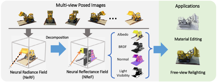
Figure 1: Given a set of multi-view posed images of an object with unknown illumination only (left-top), we estimate a neural reflectance field (NReF, mid-bottom) which decompose the neural radiance field (NeRF, left-bottom) of the object into fields of albedo, BRDF, surface normals and light visibility. NReF enables photo-realistic 3D editing tasks such as material editing and object relighting (right).

The problem of digitally reproducing, editing, and photo-realistically synthesizing an object’s 3D shape and appearance is a fundamental research topic with many applications, ranging from virtual conferencing to augment reality. Despite its usefulness, this topic is very challenging because of its inherently highly ill-posed nature and a highly non-linear optimization process, due to the complex interplay of shape, reflectance, and lighting[27] in the observations. Typical inverse-rendering approaches[13, 5, 10] rely on either dedicated capture devices, active lighting, or restrictive assumptions on target geometry and/or materials.

Recently, the pioneering work of NeRF [19] has shown great advances in 3D reconstruction from a set of posed multi-view images without additional setups. NeRF represents a radiance field for a given object using neural network as an implicit function. A radiance field is suitable for view synthesis but cannot support further manipulation tasks due to its entanglement of reflectance and lighting. To fully solve the inverse rendering problem and supports manipulation, a more suitable representation is reflectance field[4], [5], which represents shape, reflectance and lighting in a disentangled manner.

Given the surprisingly high reconstruction quality and simple cature setup of neural radiance fields (i.e., NeRF), a few recent works ([4, 24, 6, 31]) have been attempted extending neural representations to reflectance fields. Yet, some of those methods still need additional inputs such lighting information; other methods without additional input requirements, are still struggling at fully resolving the high-complexity of inverse-rendering optimization, producing noticeable artifacts and/or degenerated results. Thus, a set of questions naturally come up: Can we really achieve high quality estimation of reflectance fields with neural representations? And if possible, what is the key for an effective and robust estimation of neural reflectance fields using only posed multi-view images with unknown lighting?

In this paper, we provide positive answers to the two questions, by proposing a new method that estimates a neural reflectance field for a given object from only a set of multi-view images under unknown lighting. Inspired by[31], we formulate this problem as a two-stage optimization: An initial NeRF training stage and a NeRF decomposition stage. The pre-trained NeRF gives a plausible initialization for object shape but reflectance properties and lighting are still entangled. We then train a set of neural networks to represent implicit fields of reflectance, surface normal, and lighting visibility respectively. Fig. 1 demonstrates our idea. To avoid confusion, we will use NReF for Neural Reflectance Field afterwards.

A key challenge of decomposing neural radiance field into neural reflectance fields is to correctly extract geometry information as priors from the pre-trained NeRF. Unlike radiance fields that generate the final renderings with volumetric integration, a reflectance field only computes its rendering results on surface points of the corresponded object. Thus, a robust and accurate surface point extraction method is required for computing shading color and geometry visibility terms. However, current surface point extraction method based on volumetric density integration, using by most NeRF-based methods ([19],  [31]), often produces too surface extraction results for a robust geometry initialization, as we will shown later. To alleviate this problem, we revisit their method and amend surface the point extraction process by proposing an effective strategy based on ray-casting. To support fast point querying during training, we construct an octree on densely sampled point cloud from NeRF.

The second key challenge of high-quality neural reflectance field optimization under unknown lighting is to resolve ambiguities due to its intrinsically ill-posed nature. Previous image-based reflectance decomposition methods ([2]) have shown that adding suitable smoothness and parsimony prior terms is crucial to resolve shading/albedo ambiguity. Our key observation is that, adding different type of priors mentioned above during training, can be unified as applying different type of filters on the geometry surface. However, applying such filters are non-trivial for neural reflectace field as the surface are only defined with implicit functions. To address this issue, we exploit the idea of Gaussian KD-tree ([1]) to efficiently compute a discrete sampled approximation of all prior terms, and employ a commitment loss to propagate the prior back into the implicit fields. In this way, we are able to add suitable priors for decomposing reflectance and shading and significantly improving the quality of neural reflectance field estimation.

Based on the two auxiliary tree-based data structures, we design an optimization pipeline with carefully considerations on surface extraction, prior terms, and importance sampling of lighting. Our pipeline enables the estimation of high-quality neural reflectance fields with only multi-view posed images under unknown lighting as input. We validate and demonstrate the strength of our method with extensive experiments on both synthetic and real data. We also apply our method to manipulation tasks such as relighting and material editing.

To summarize, our contributions are as follows:

• A novel approach for estimating reflectance field of 3D objects using only multi-view posed images under uncontrolled, unknown lighting.

• A new method to extract surfaces point from pre-trained radiance fields with reduced noise.

• A dedicate designed optimization pipeline that decomposes a neural radiance fields into neural reflectance fields to support manipulation tasks.

2 Related Works

Inverse Rendering. The task of inverse rendering is to decompose an observed image of a given object into geometry, appearance properties and lighting conditions, such that the components follow the physical imaging process. Since the decomposition is intrinsically an ill-posed problem, most prior approaches address this problem by adding strong assumptions on object shape ([2, 15, 28, 11, 16, 8]), exploiting additional information of shape or lighting ([9, 24, 5]), or designing dedicated devices for controllable capturing ([13, 18]). Our method only uses multi-view images as input and has less restriction on shapes/materials.

Neural 3D Representations. Recently, the neural representation of 3D scenes has attracted considerable attention in the literature([19, 3, 23, 22, 7]). These methods exploit multi-layer perceptrons to represent implicit fields such as sign distance functions for surface or volumetric radiance fields, known as Neural Fields. Our method builds upon the neural radiance field (NeRF) for 3D representation. NeRF [19] and its variants have surpassed previous state-of-the-art methods on novel view synthesis tasks; however, NeRF cannot support various editing tasks because it models radiance fields as a “black-box”. Our work takes one step further towards opening this ”black-box” by providing a method to decompose NeRF into shape, reflectance and lighting, enabling editing tasks. Some prior arts also attempt to model reflectance fields with neural networks. NeRV [24] proposed a method that estimates reflectance fields from multi-view images with known lighting. Bi et el. [4] estimate reflectance fields from images captured with a collocated camera-light setup. Our method does not require lighting conditions as prior information. NeRD [6] and PhySG [30] directly solve reflectance fields from multi-view posed images with unknown illumination. Both NeRD and PhySG do not take light visibility into account and are unable to simulate any lighting occlusion or shadowing effects. We address this issue by modeling the light visibility field in our decomposition. The most similar work to us is NeRFactor [31] which also decomposes a reflectance field from a pre-trained NeRF. A key drawback of NeRFactor is their limited quality. Overall, NeRFactor tends to output over smoothed normal, less disentangled albedo/shading, and degenerated specular components. Our method greatly improve the quality of neural reflectance field by improving the surface point extraction, correctly handling dynamic importance sampling, and adding additional priors. These improvements cannot be trivially implemented without our introducing of tree-based data structures and carefully designed training strategies.

Data structures for neural representations. The octree data structure have been used in several works to accelerate training and/or rendering of neural radiance fields ([17], [29]). The method of Gaussian KD-Tree [1] has been used for accelerating a broad class of non-linear filters that includes the bilateral, non-local means, and other related filters. Both data structures plays an important role in our method during NReF training: the octree gives us the ability to query extracted surface points on the fly for computing geometric visibility terms, and the Gaussian KD-tree enables us to apply different prior term in a unified way by filtering high-dimensional features on object surfaces.

3 Method

Our goal is to estimate a neural reflectance field (NReF), given only $n$ multi-view posed images $\{I_{k}|k=1...n\}$ with unknown lighting as observations. A NReF $f(\mathbf{x})$ represents the shape, light, and reflectance properties of an object at any 3D location $\mathbf{x}$ on its opaque surface. We parameterize NReF with a set of multi-layer perceptron (MLP) networks and solve the NReF estimation with a ‘NeRF decomposition’ approach. A NeRF MLP is first is trained with the same set of inputs (section 3.1) and the initial surface geometry is extracted from it with a novel ray-casting based approach, accelerated with octree (section 3.2). The decomposition itself relies on a set of priors to resolve ambiguities that are non-trivial to employ with neural implicit field representations only. We address this issue with a Gaussian KD-tree that converts priors into surface filtering operations (section 3.3). Finally, we introduce our multi-stage NReF decomposition pipeline with implementation details (section 3.4).

3.1 From Radiance to Reflectance

We begin by training a Neural Radiance Field (NeRF) following the same procedure in [19]. In NeRF, the rendered color $C(\mathbf{r})$ of the camera ray $\mathbf{r}(t)=\mathbf{o}+t\mathbf{d}$ is generated by querying and blending the radiance $L_{o}(\boldsymbol{\omega}_{v},\mathbf{r}(t))$ according to the volume density value $\sigma(\mathbf{r}(t))$ alongside $\mathbf{r}$(t) via

$$C(\mathbf{r})=\int_{0}^{\infty}\frac{\partial T(\mathbf{r}(t))}{\partial t}L_{o}(\boldsymbol{\omega}_{v},\mathbf{r}(t))dt$$ (1)

where

$$T(\mathbf{r}(t))=1-\exp\left(-\int_{0}^{t}\sigma(\mathbf{r}(t))ds\right)$$ (2)

Here, $\boldsymbol{\omega}_{v}=-\mathbf{d}/\lVert\mathbf{d}\rVert$ is the normalized view direction, and $T(\mathbf{r}(t))$ is the transmittance function. NeRF works well for view synthesis since it already learned reasonable shape via the volume density $\sigma(t)$; however, it is not suitable for other manipulations of shading effects because reflectance and lighting are still entangled. To enable control over those factors, we formulate a decomposition problem for estimating NReF as follows.

Reflectance field formulation  The relationship of radiance, shape, reflectance, and lighting at surface point $\mathbf{x}$ from direction $\boldsymbol{\omega}_{v}$ is given by the rendering equation ([12]):

$$L_{o}(\boldsymbol{\omega}_{v},\mathbf{x})=\int f_{r}(\boldsymbol{\omega}_{v},\boldsymbol{\omega}_{i},\mathbf{x})L_{i}(\boldsymbol{\omega}_{i},\mathbf{x})\max(f_{n}(\mathbf{x})\cdot\boldsymbol{\omega}_{i},0)d\boldsymbol{\omega}_{i}$$ (3)

where $f_{r}(\cdot)$ is the Bidirectional Reflectance Distribution Function (BRDF), $L_{i}(\boldsymbol{\omega}_{i},\mathbf{x})$ is the incident light at direction $\boldsymbol{\omega}_{i}$ and $f_{n}(\cdot)$ is the surface normal. We further assume light sources are far-field and decompose the lighting $L_{i}(\cdot)$ into a directional environment map $L(\boldsymbol{\omega}_{i})$ and a light visibility term $f_{v}(\mathbf{x},\omega_{i})$,

$$L_{i}(\boldsymbol{\omega}_{i},\mathbf{x})=f_{v}(\boldsymbol{\omega}_{i},\mathbf{x})L(\boldsymbol{\omega}_{i})$$ (4)

A straightforward way to estimate the NReF is by simply inserting equ. 3 into equ. 1 and minimizing the render loss with image observations. However, simultaneously estimating all components of NReF from scratch is extremely hard and unstable due to its ill-posedness nature, even under known illumination conditions [24]. Fortunately, the NeRF has already decomposed geometry information to some extent and we can extract an initial surface $\mathbf{S}$ from it. Given this, the rendering loss $\mathcal{R}(\mathbf{r})$ can be then greatly reduced to first query the surface point $\mathbf{x}_{s}$ and then evaluate equ. 3 on it:

$$\mathcal{R}(\mathbf{r})=\mathcal{R}(\boldsymbol{\omega}_{v},\mathbf{x}_{s})=\lVert I(\mathbf{r})-L_{o}(\boldsymbol{\omega}_{v},\mathbf{x}_{s})\rVert^{2}_{2}$$ (5)

The numerical method for approximating the integral of equation 3 plays a crucial role during the optimization. Previous neural reflection field estimation method ([31], [24]) approximate the integration with a pre-defined equirectangular map of lighting directions. However, we argue that this simple strategy is far from an optimal one ([25]). In particular, this sampling strategy is not only biased but also gives significant noisy results with an affordable amount of samples during training. Naively increasing number of samples leads to unacceptable memory and time cost. We address this issue by following the standard importance sampling strategy [25] in physical-based rendering field. The importance sampling directions are calculated based on the material roughness properties.

3.2 Extracting geometry priors from NeRF

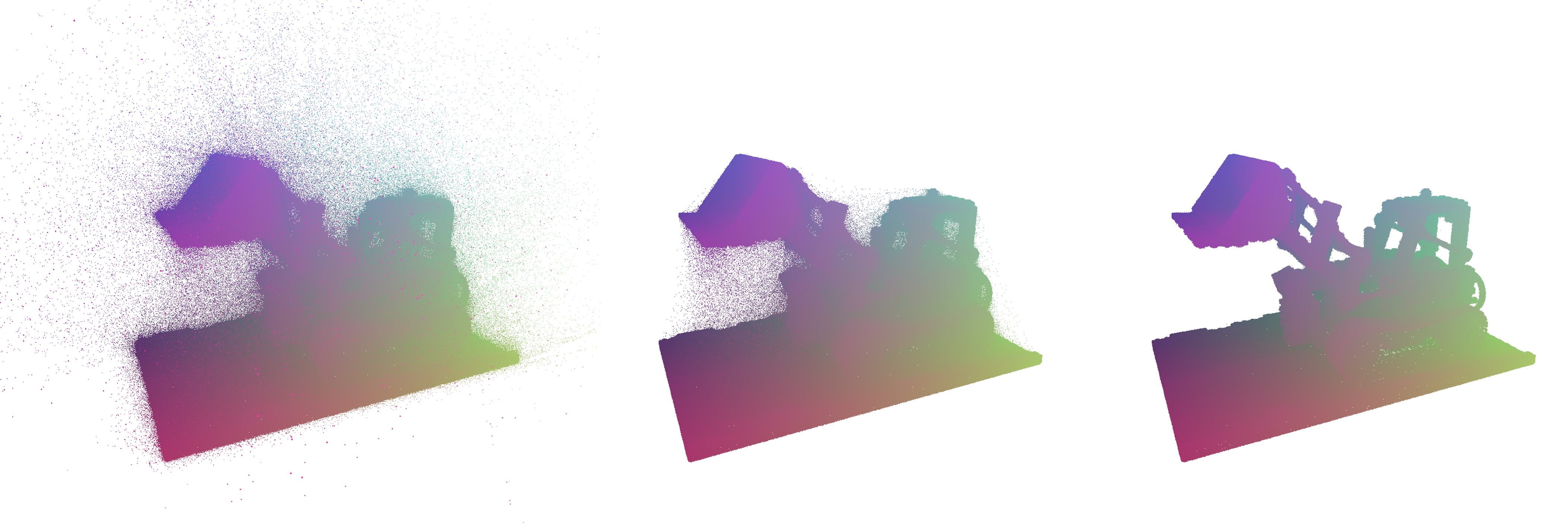
Figure 2: The improvement of surface extraction. Left: surface extraction result with equation 6 produces many erratic scattered points. Middle: A slightly improved version of equation 6 by normalizing weight still produces scattered points. Right: Our surface extraction method with equation 7 removes almost all outlier points.

Surface points and normals  The original NeRF suggests extracting surface points along a single ray $\mathbf{r}(t)$ with its expected termination:

$$\mathbf{x}_{s}=\int_{0}^{\infty}\frac{\partial T(\mathbf{r}(t))}{\partial t}\mathbf{r}(t)dt$$ (6)

The surface normal at $\mathbf{x}_{s}$ can be computed as the negative normalized gradient of NeRF’s density output $\sigma(t)$ w.r.t point positions via auto-differentiation [24][31]. In practice, however, we observe that the surface and normal derived from equ. 6 is usually noisy and erratic, as shown in fig 2 and fig 5. The reason is that the density field from NeRF actually tends to ‘fake’ glossy surfaces by creating two or more small layers, thus naively blend them along ray directions will create ‘fake’ floating points. The detailed analysis of failure cases of equ. 6 are given in the supplementary material. To alleviate this, we employ an empirical but effective strategy by simply finding the point $\mathbf{x}_{s}$ on the ray that satisfies

$$T(\mathbf{r}(s))=\frac{T(\mathbf{r}(t_{n}))+T(\mathbf{r}(t_{f}))}{2}$$ (7)

where $t_{n}$ and $t_{f}$ are the ray-tracing bound. Unlike equ 6 which spreads floating points along the ray, extracting points with equ 7 will force the points distributed on one of the surface layers. As $T(\cdot)$ is a monotonic function by definition, there is always a unique solution for equ. 7 and we found it works well in practice, as shown in fig 2. Given the surface point $\mathbf{x}_{s}$, we extract its normal directions by averaging the density gradient around a small region centered at $\mathbf{x}_{s}$ weighted by its density value to further reduce the normal noise.

Light visibility  The light visibility at surface point $\mathbf{x}_{s}$ can be calculated as integrating the $T(\cdot)$ defined in equ.2 on the normal-directed hemisphere. Since we have built an octree to store the density field on the surface points, we again utilize it to compute the integration dynamically with importance sampling strategy during the optimization. Note that the octree not only supports light visibility query on the fly, but also enables efficient depth estimation during the rendering.

NeRF commitment  During the decomposing process, the surface normal and light visibility of NReF will be refined by the render loss. Yet, the predicted normal and light visibility should not derive too much to that of NeRF. Thus, we add a NeRF commitment loss to constrain the optimized normal and visibility close to NeRF on the extracted surface points,

$$\mathcal{C}_{f_{\theta}}(\mathbf{x_{s}})=\lVert f_{\theta}(\mathbf{x}_{s})-F(\mathbf{x}_{s})\rVert^{2}_{2}$$ (8)

where $f_{\theta}(\cdot)$ and $F(\cdot)$ denote corresponding components (normal or visibility) of NReF and NeRF respectively, $\theta$ indicates the dependence of network parameters of NReF.

3.3 Enforcing Smooth and Parsimony

For estimating reflectance under unknown illumination, other priors are necessary. We employ two well-known prior knowledge from the intrinsic decomposition literature [2]: the predicted normal, visibility and BRDF should be locally smooth, and the albedo color should be globally sparse. These priors can be unified into one single formulation as applying filter operations on the surface points (the derivation and normalizing term have been dropped for simplification):

$$f_{\mathcal{P}}(\mathbf{x}_{i})=\sum_{j\neq i}k(\mathbf{v}_{i},\mathbf{v}_{j})f_{\theta}(\mathbf{x}_{j})$$ (9)

where $k(\mathbf{v}_{i},\mathbf{v}_{j})$ denotes the weight from $\mathbf{x}_{j}$ to $\mathbf{x}_{i}$, based on the similarity of a high-dimensional vector $\mathbf{v}$ defined on the surface. The form of $\mathbf{v}$ is related to different prior types. Specifically, for local smoothness term, $\mathbf{v}$ is defined as the bilateral kernel weight:

$$\mathbf{v}_{i} =(\mathbf{x}_{i},f_{\theta}(\mathbf{x}_{i}))$$ (10)

$$k(\mathbf{v}_{i},\mathbf{v}_{j}) =\exp(-|\mathbf{v}_{i}-\mathbf{v}_{j})|^{2})$$ (11)

$$=\exp(-|\mathbf{x}_{i}-\mathbf{x}_{j}|^{2})\exp(-|f_{\theta}(\mathbf{x}_{i})-f_{\theta}(\mathbf{x}_{j})|^{2})$$ (12)

For global sparsity (also known as parsimony in [2]), $\mathbf{v}$ contains only the albedo color, i.e., $\mathbf{v}_{i}=f_{\theta}(\mathbf{x}_{i})$. During training, priors are enforced by first applying filter operations with equ. 9, then minimizing the difference between the NReF $f_{\theta}(\cdot)$ and its filtered version $f_{\mathcal{P}}(\cdot)$:

$$\mathcal{P}_{f}(\mathbf{x}_{i}) =\lVert f_{\mathcal{P}}(\mathbf{x}_{i})-f_{\theta}(\mathbf{x}_{i})\rVert$$ (13)

$$=\lVert\sum_{j}k(\mathbf{v}_{i},\mathbf{v}_{j})(f_{\theta}(\mathbf{x}_{j})-f_{\theta}(\mathbf{x}_{i}))\rVert$$ (14)

$$\approx\sum_{j}k(\mathbf{v}_{i},\mathbf{v}_{j})\lVert f_{\theta}(\mathbf{x}_{j})-f_{\theta}(\mathbf{x}_{i})\rVert$$ (15)

Computing priors with Gaussian KD-Tree  In practice, we calculate the prior terms using the Gaussian KD-Tree [1]. A high-dimensional KD-Tree is constructed on point set of vector $\mathbf{v}$. To calculate the prior loss, instead of directly apply filtering and storing the filtered values $f_{\mathcal{P}}$, we approximate it stochastically by using an importance sampling of $\mathbf{x}_{j}$ proportionally to $k(\mathbf{v}_{i},\mathbf{v}_{j})$ in each mini-batch (see equ. 15), and asynchronously updating the KD-tree to reflect changes of $\mathbf{v}$ every epoch. For parsimony term, we further reduce the computational cost by employ a K-means operation on the albedo colors and randomly keep several points in each cluster as the candidate $\mathbf{x}_{j}$.

3.4 Multi-stage Optimization

Per equation 5, 8 and 13, the final loss used to decompose NReF from NeRF is:

$$\mathcal{L}=\lambda_{r}\mathcal{R}+\lambda_{c}\mathcal{C}+\lambda_{p}\mathcal{P}$$ (16)

To avoid optimizing a too complicated target space, we split the NReF decomposition into multiple sub-stages as follows (more details in the supp. material):

Pre-training NeRF  We use the same network structure and follows the training strategy from [19] for pre-training NeRF. We train NeRF for 2000 epochs with randomly sampling 1024 camera rays for each image per mini-batch.

Training normal and visibility  Given a pre-trained NeRF, we firstly extract the surface points and normal using equ. 7. An octree is constructed on the surface points and the light visibility is computed on the fly during training. We train the normal and visibility component for 100 epochs. During training we filter out few points that still have erratic normal directions our refined surface extraction by discarding their commitment loss and additionally add a visibility loss to predicted normal w.r.t. its view direction.

Joint optimization  After the normal and visibility training, we have had a quite reasonable geometry initialization for NReF. To prevent the uninitialized material properties and env. lighting ruin out the geometry at the beginning, we apply a warm-up stage during which we use large geometry commitment weight $\lambda_{c}$ and small smoothness and parsimony weight $\lambda_{p}$. We warm-up the training for 100 epochs and then joint train all components with equ. 16 for another 200 epochs with all terms properly applied.

Implementation details  We model the BRDF $f_{r}(\cdot)$ as a lambertian diffuse part with albedo color $f_{a}(\mathbf{x})\in R^{3}$ plus a specular part with GGX Microfacet model [26] that is controlled with roughness parameter $f_{s}(\mathbf{x})\in[0,1]$. The albedo $f_{a}(\mathbf{x})$, roughness $f_{s}(\mathbf{x})$, normal $f_{n}(\mathbf{x})$, and visibility $f_{v}(\mathbf{x},\omega_{i})$ are all parameterized with MLP network of 4 layers. The environmental map $L(\boldsymbol{\omega}_{i})$ is represented with a cube map texture. We build a mipmap over the cubemap and sample the corresponding mipmap level according to the PDF of sampled light directions [20] using soft rasterization [14]. For computing equ. 3, we sample 128 rays w.r.t the estimated roughness and 64 rays with uniform sampling. We set $\lambda_{r}=1.0$; the weight $\lambda_{c}$ is set to 0.5 during the warm-up training, and reduced to 0.1 in the final joint training stage. The weight $\lambda_{p}$ for albedo/roughness/shape smoothness is set to 0.5/0.01/0.1, and 0.1/0.005 for albedo/roughness parsimony.

Computational cost  The whole training can be conducted on a single NVidia Tesla V100 GPU. The total training time for $512\times 512$ resolution with $100$ views is approximately 15 hours, with 14 hours for NeRF pre-training, 15 minutes for training normal and visibility, and another 30 minutes for joint optimization. For inference, rendering one image of $512\times 512$ takes around 8 seconds with a typical importance sampling setup of 64 diffuse samples and 128 specular samples.

4 Experiments

To validate our proposed method, we first perform ablation studies on our revised geometry extraction method and different prior terms enabled by octree and Gaussian KD-tree (sec. 4.1). We also perform comparisons against related methods and show our advantage (sec. 4.2). Finally, we show more results on real data and demonstrate manipulation applications enabled by NReF (sec. 4.3).

Datasets  The ablation studies and comparison with [31] and [24] is evaluated on the synthetic Blender scenes released by Mildenhall et al. ([19]). In [31] the author re-render the synthetic Blender scenes with their own illumination conditions. We compare our results using their rendering setup for a fair comparison. The comparison with [27] is evaluated on their real captured dataset. Results on other real data is generated from mobile phone captured data released by [19].

4.1 Ablation Studies

In this section we ablation each component in our optimization pipeline that contributes to the final high-quality reflectance field results.

Geometric-aware smoothness term   A significant advantage of our method is the geometric-aware smoothness enabled by bilateral normal filtering with Gaussian KD-tree. We validate the gain from this advantage in fig. 3 by removing the smoothness term, or replacing it with a naive smoothness term in euclidean space (i.e., similar to [31]). Without geometric-aware smoothness, the geometry features tend to be either too noisy (w/o smoothness at all) or smoothed out together with noise.

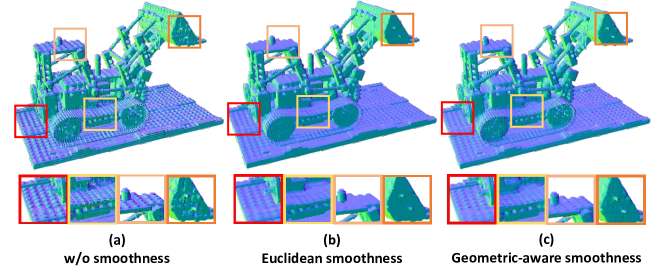
Figure 3: The effect of smoothness term. (a) without any smoothness constraint, the trained normal is sensitive to noisy points (e.g., the tiny lego bumps, highlighted in red) (b) directly adding smoothness in euclidean space remove most noise; however, it also tends to smooth out geometry details. (c) adding geometric-aware smoothness removes noisy normal while preserves shape details.

Global parsimony term

Figure 4: The effect of parsimony term. (a) the shading effect is hard to disentangled from albedo without a parsimony prior. (b) the parsimony term enforces a piecewise-constant albedo and remove most shading. Note for the bottom case our method (b) fails to completely produce a single color for the plate due to strong inter-reflection that cannot be handled in our formulation. Yet, we still remove most shadow caused by shading compared to (a).

Our method also enables global prior terms that cannot be applied in previous works [24],[31]. We show the benefit of our global parsimony term in fig. 4. The global parsimony provides a strong color-sparsity constraint on the albedo field and prevents incorrect shading effects baking in.

Improvements over NeRF normals

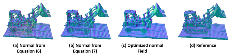
Figure 5: The improvement over NeRF normal. (a) Initial normal extracted with Equation 6 is extremely noisy and erratic such as the track region. (b) Initial normal extracted with Equation 7 improves the normal and provides a good initialization point. (c) Our optimization further improve the normal with significant noise reduction while preserves geometry features. The reference normal is shown in (d).

We compare and validate our effects of better normal initialization as well as normal optimization results in fig. 5. The initial normal extracted with equ. 6 is extremely noisy (e.g., the track region). Our method extracts a cleaner initialization with equ. 7 and the results are further improved after the optimization.

4.2 Comparisons

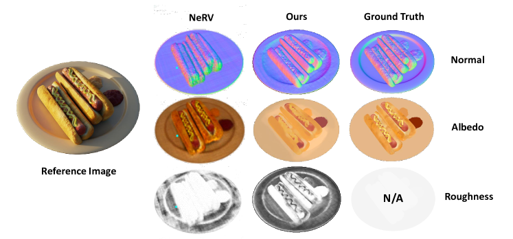
Figure 6: Comparison with NeRV [24]. NeRV (left) produce incorrect normals and noisy roughness on the plate part, with a large ratio of shading baked into albedo. Our result (middle) produces correct normal for the plate, remove most shading from albedo and produces a reasonable roughness with glossy material for the plate and rough material for the hotdog. One example view of the input image is shown on the left for reference to illustrate the strong inter-reflection in this data.

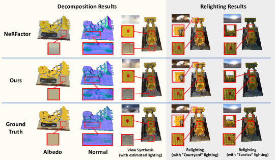
Figure 7: Compared with NeRFactor [31], our method estimates a cleaner albedo with less shading bake in, a more detailed normal without introducing noise, and more plausible lighting conditions. Our method also renders novel images that better reproduces geometry details and lighting effects. The lighting estimated from input and used for re-rendering are shown on the left-top of corresponding images.

Method	Normal (Degree)$\downarrow$	Albedo (PSNR)$\uparrow$	View Synthesis (PSNR)$\uparrow$	Relighting (PSNR)$\uparrow$
NeRFactor[31]	22.1327	28.7099	32.5362	23.6206
NeRFactor*	29.0603	22.1496	24.8610	19.0691
Ours	30.1381	24.0959	27.2362	20.5153

Table 1: Quantitative comparison with NeRFactor. We found that the original implementation of NeRFactor computes the PSNR in grayscale color space and did not remove the black backgrounds, leading to lower errors on all scenes. For fairness, we list both their reported values (first row) and re-computed values in RGB with only object foreground (second row). Our method (bottom row) exhibits a significant PSNR improvement (1.95db/2.38db/1.45db) for albedo and novel synthesized image with refined metric. NeRFactor have a slightly lower normal error (1.07^∘) than us, but visually we found our method produce more detailed results on normal map (fig 7).

Comparisons with other neural reflectance field  We compare our methods with two methods that share a similar setup: NeRFactor [31] and NeRV [24]. NeRV [24] directly train everything from scratch without employing a NeRF pre-training stage, leading to a too complicated optimization problem that often fall into local minima with less plausible visual quality, as shown in fig. 6. NeRFactor [31] formulates the problem similar to us by first pre-training a NeRF and then conducting decomposition. However, without tree-based structures as support, their method is optimized without a dedicated consideration on surface point extraction, suitable prior terms, and sampling strategies. Thus, it suffers both smoothness and parsimony issues as discussed in sec. 4.1, producing over-smoothed normal field as well as less cleaned albedo field, and often degenerates to a near-diffuse decomposition result. Our method address all the above issues and outperforms NeRFactor, both quantitatively (tab. 1) and qualitatively (fig. 7).

Comparison with non-neural method  We compare our method on real captured data with a high-quality non-deep learning method [27] that reconstruct shape, appearance and lighting from image sequences. Fig 8 shows a qualitative comparison result. As reported in [27], their results were generated with a 20 node PC cluster using a total of 1243 captured images. Our method reduced the number of images needed (500 images for this experiment) and can be conducted on a single PC with one GPU card. Overall, the quality of our results are similar to [27] with significantly reduced number of inputs and computational cost.

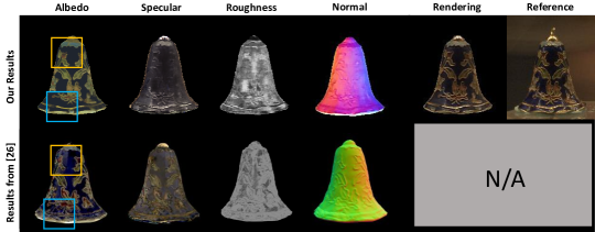
Figure 8: Qualitative comparison with [27] on the real captured ”Cloisonne Bell” data from [27]. Note that [27] used a different BRDF model thus the absolute value of roughness and specular are not comparable, and [27] use a different color maps for normal visualization. Overall, our method (top row) produces a cleaner albedo (highlighted with yellow rect.) with less specular baked-in (highlighted with blue rect.) than [27] (bottom row). [27] produces visually cleaner roughness than ours. Yet, both method produce a visually plausible specular components and our rendering results are plausible comparing with the reference image.

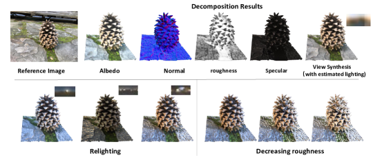
Figure 9: NReF estimation on real captured data. Left: One of the input views for reference. Upper row: decomposed albedo, normal and novel view synthesis with estimated lighting on the right. Lower row: relighting and changing roughness.

4.3 Results and Applications

We further demonstrate our method’s ability to estimate NReF as well as its applications for manipulation tasks on real-world captured multi-view images. Fig 9 shows our decomposed NReF components, view synthesis, relighting, and material editing results. Our method estimates plausible reflectance field decomposition and enables photo-realistic editing results. Additional results, including videos of relighting and view synthesizing, are given in the supp. material.

5 Conclusion

We presented a new method for estimating the Neural Reflectance Field (NReF) of objects that only requires a set of multi-view images under unknown lighting. Our method is built upon a multi-stage training pipeline that decomposes a pre-trained NeRF into NReF. The key to enable our high quality decomposition is a new method of surface point extraction from NeRF with a dynamic importance sampling strategy supported by octree, and a Gaussian KD-tree based method to apply suitable prior terms. We demonstrated the robustness and effectiveness of our method on both synthetic and real data. Our estimated NReF can be used for manipulation tasks such as relighting and material editing.

Limitations Our method is not without limitations. NReF only optimizes a normal field that is defined on the surface of the origin NeRF shape. Thus NReF might fails if the NeRF shape deviates too much from ground truth. Our method currently assumes opaque surfaces of isotropic materials without inter-reflections, and might produces artifacts for inputs with violation. Visualizations of some typical failure cases are given in the supplemental material.

Future works Avenues for future works include removing camera pose requirements as input, supporting geometry refinement during training, handling inter-reflections, and extending our method to dynamic scenes.

This appendix provide more implementation details, additional evaluations and discussions.

Appendix A Implementation

A.1 Network Structure

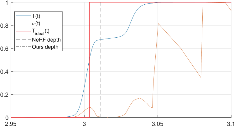
Figure 10: $T(t),\sigma(t)$ at a zooming region around the surface, along a single ray direction parameterized by $t$. The orange curve shows the density along side the ray. Notice that there is a small vacuum region between depth at 3 and 3.05. Using Equ.6 in the main paper will put the depth (the dashed line) at this region where the gradient of the density is not well defined, i.e. nearly zero. Using our method (Equ.7) will extract a depth point with well-defined gradient (the dot dashed line.

NReF consists of 4 sub-networks that correspond to output surface albedo color $\rho_{d}\in\mathbb{R}^{3}$, surface roughness value $\rho_{r}\in(0,1)$, surface normal direction $n\in\mathbb{R}^{3}$, and light visibility $v\in\{0,1\}$ respectively. Each sub-network is modeled with an MLP network with 4 fully-connected layers with 128 hidden units and ReLU activation function. The input of albedo, roughness, and normal is point position $\mathbf{x}\in\mathbf{S}$ on the surface. The light visibility takes both point position and incident lighting direction $\boldsymbol{\omega}_{i}$ as input by simply concatenating them. Overall, we keep our network design the same as NeRFactor [31], except for the BRDF component for which we use an analytical BRDF model instead of a pretrained one. We follow the same approach of applying positional encoding to the input as the majority of NeRF-related work does.

Our pre-trained NeRF for volume density is exactly the same structure described in [19] with 8 layers of MLP, each with a width of 256 hidden units and ReLU activation. A skip connection at the 4th layer is also included. Figure 11 details the network structures of NeRF and NReF used in this paper.

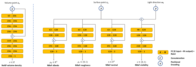
Figure 11: Our network structure for NeRF and NReF.

A.2 Environment lighting.

We model the far-field lighting condition as a cube map during training. To improve sampling efficacy and rendering quality, we construct a mip-map [20] for the cube map. The mipmap is sampled using using NVDiffrast [14]. The mipmap level for a given light ray is calculated as

$$l=\max\left(\frac{1}{2}\log_{2}\frac{\Omega_{s}}{\Omega_{p}},0\right)$$ (17)

Here $\boldsymbol{\Omega}_{s}$ is the solid angle of sampled rays direction, which is

$$\Omega_{s}=\frac{1}{Np(\boldsymbol{\omega})}$$ (18)

where $N$ is the number of samples, and $p(\boldsymbol{\omega})$ is the pdf.

$$\Omega_{p}=\frac{4}{W^{2}}\partial A$$ (19)

$$\partial A=\frac{1}{(u^{2}+v^{2}+1)^{3/2}}$$ (20)

where $u,v\in[-1,1]$ is the projected coordinated of $\boldsymbol{\omega}$, and $W$ is the resolution of base mipmap level. We add additional lighting smooth loss by minimizing the residual between mipmap level 0 and 1.

Appendix B Additional Evaluation

B.1 Surface Extraction from NeRF

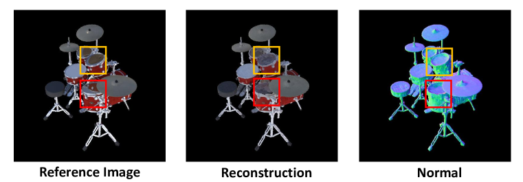
Figure 12: A failure case. Red box: the initial surface from NeRF incorrectly put the bottom part of the drum on the top, and NReF failed to fix this with normal variation only. Yellow box: the top part of the drum is a glass-like transparent surface which violates our opaque surface assumption. Note the original data provided in [31] masked out the bottom part of the drum in the red box and produces a hollow albedo in that region; we keep this part of mask in this figure to show a typical failure case only.

The initial surface normal induced by the surface extraction method in [19][31] (Equ.6 in the main paper) is often noisy and erratic. The reason is that the original shape inducted from NeRF inevitably creates small, double-layered translucent surfaces with vacuumed density in-between, which violates the assumption of opaque surfaces. This phenomenon itself, and how it affects the normal induction, are illustrated in figure 10. In theory, an opaque surface should have a step-wise transmittance function along the ray direction (red curve $T_{ideal}(t)$ in fig. 10) where the step-change point corresponds to the surface point. In practice, due to the intrinsic entanglement of surface geometry and view-dependent color effects, the transmittance function trained by NeRF usually comes up with two smaller ”step-wise” transitions close to each other (blue curve in fig. 10) to compensate for view-dependent color effects. The two smaller ”step-wise” transitions of NeRF corresponds to a double-layered translucent surface locally. Applying Equ.6 in such a case will scatter bad approximation of surface points at the middle vacuumed region. These scattered points not only produces noisy surface points itself, but also provides noisy and erratic normal because points in this region usually have a small, unstable gradient towards zero. Our idea to address this issue is simple - we just make sure the approximated surface point stops at one of the two step-changed points by raymarching with Equ.7 in the main paper. In another word, we find the surface point by performing ray-marching until the transmittance equals to $0.5$. Since both step-changed points have a well-defined gradient, we can extract a more reasonable surface normal.

B.2 Parsimony Prior

Our parsimony term enables long-range/global color similarity. This is demonstrated in Fig. 13.

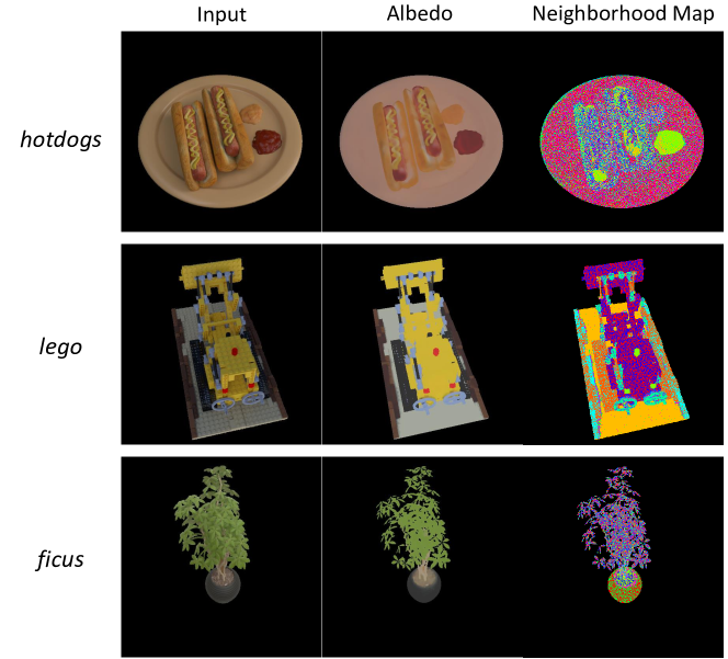
Figure 13: Visualization of the parsimony prior. Left column: input image for reference. Middle column: decomposed albedo map. Right column: visualization of sampled sparse neighbors for each point. The cluster of sampled neighbor is encoded as hsv colors. The noise is due to stochastic sampling.

Appendix C Additional Results

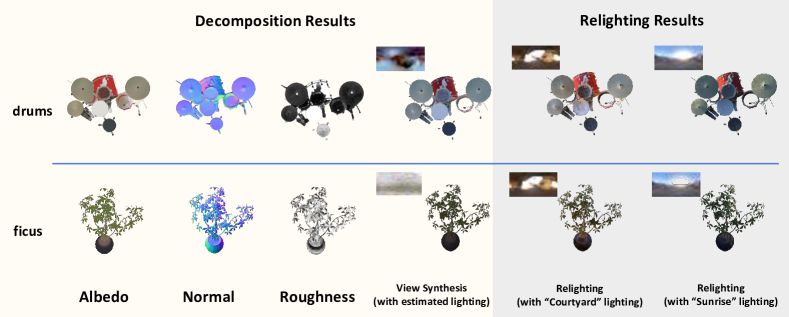
Figure 14: Our full decomposition, reconstruction, and novel relighting results.

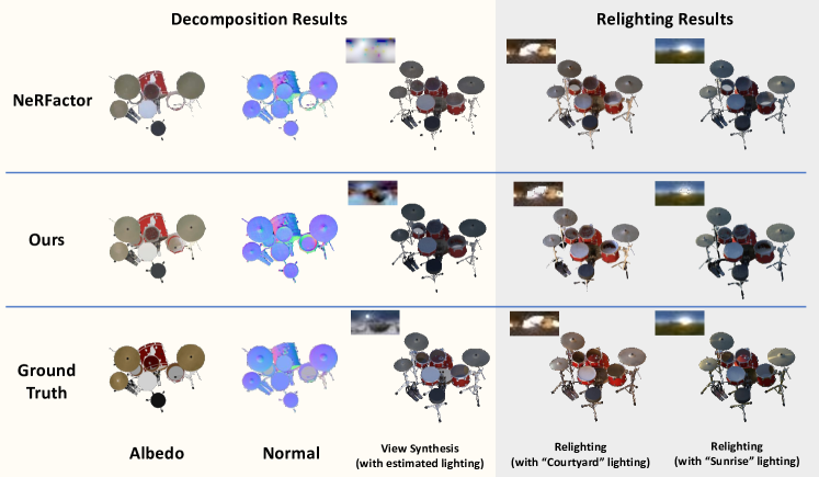
Figure 15: Comparsion of our method with NeRFactor and ground truth on drums synthetic data.

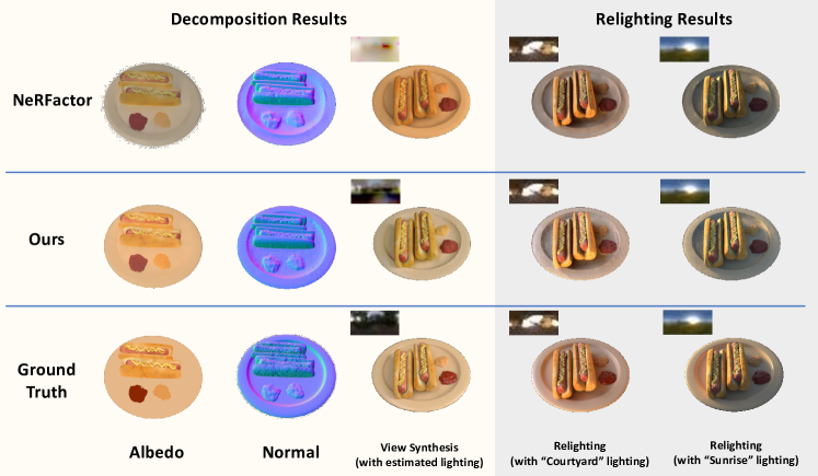
Figure 16: Comparsion of our method with NeRFactor and ground truth on hotdog synthetic data.

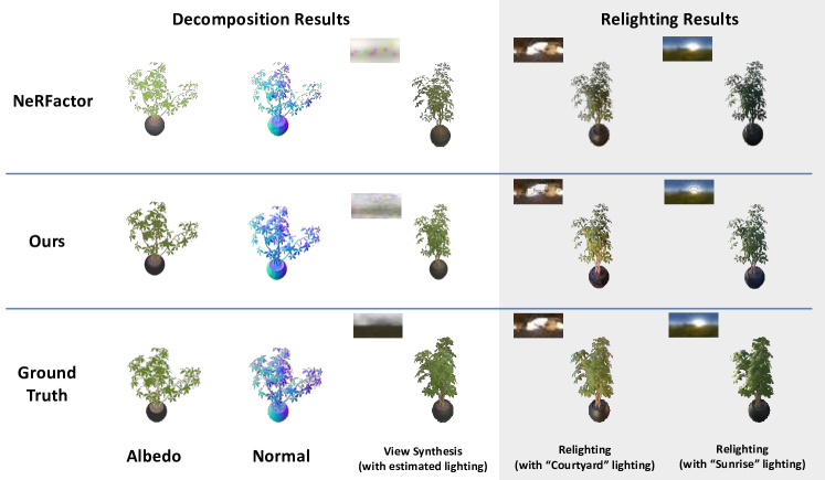
Figure 17: Comparsion of our method with NeRFactor and ground truth on ficus synthetic data.

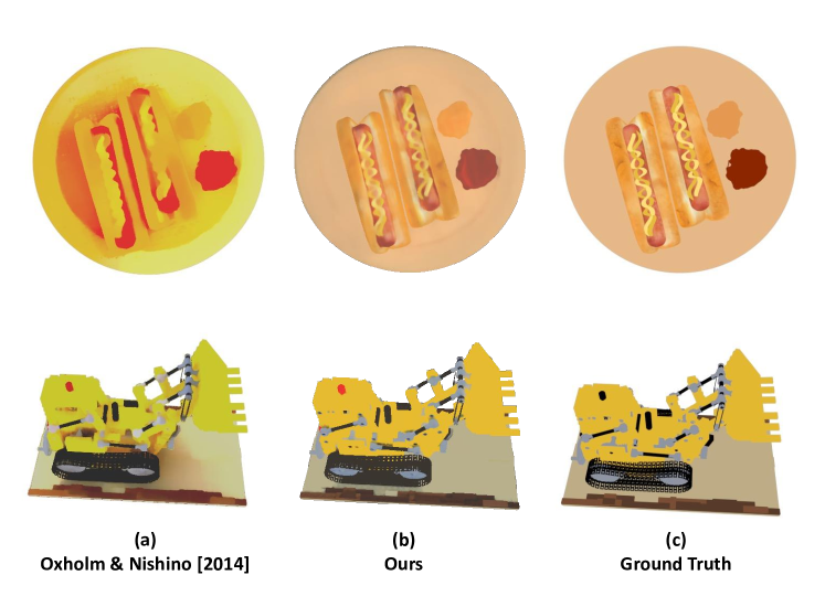
Figure 18: Qualitative Comparison with Oxholm and Nishino [21]. For a fair comparsion, we compare our method with the multi-view enhanced version of [21] from NeRFactor [31]. Our method produce significantly better albedo estimation results with less artifacts.

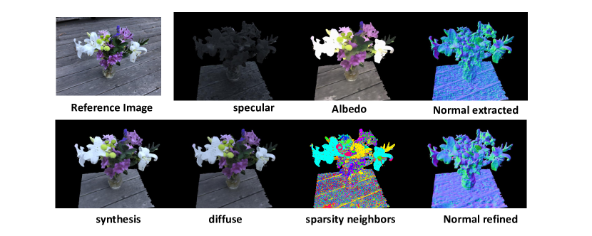
Figure 19: Our full decomposition, reconstruction results on another real captured data.

Here we show additional results on other synthetic data released by [19] (Fig. 14) that are not shown in the main paper, as well as more side-by-side comparison (Fig. 15,  16, and 17) with NeRFactor [31] and ground truth. We also compare our method with previous method of multi-view photometric stereo [21] in fig. 18. Additional results on real-captured data is shown in fig. 19.

C.1 Failure cases.

Our method have a set of assumptions for input, including opaque objects, isotropic materials, inter-reflections free, etc. Violating those assumptions might produces incorrect results. The NReF relies on initial surfaces extracted from NReF and only refines normal but not surface positions; thus a strongly deviated shape might not be able to be fixed and produces artifacts. A typical failure case is shown in Fig 12.

References

- [1] Andrew Adams, Natasha Gelfand, Jennifer Dolson, and Marc Levoy. Gaussian kd-trees for fast high-dimensional filtering. In ACM SIGGRAPH 2009 papers, pages 1–12. 2009.
- [2] Jonathan T. Barron and Jitendra Malik. Shape, illumination, and reflectance from shading. TPAMI, 2015.
- [3] Jonathan T Barron, Ben Mildenhall, Matthew Tancik, Peter Hedman, Ricardo Martin-Brualla, and Pratul P Srinivasan. Mip-nerf: A multiscale representation for anti-aliasing neural radiance fields. arXiv preprint arXiv:2103.13415, 2021.
- [4] Sai Bi, Zexiang Xu, Pratul Srinivasan, Ben Mildenhall, Kalyan Sunkavalli, Miloš Hašan, Yannick Hold-Geoffroy, David Kriegman, and Ravi Ramamoorthi. Neural reflectance fields for appearance acquisition. arXiv preprint arXiv:2008.03824, 2020.
- [5] Sai Bi, Zexiang Xu, Kalyan Sunkavalli, Miloš Hašan, Yannick Hold-Geoffroy, David Kriegman, and Ravi Ramamoorthi. Deep reflectance volumes: Relightable reconstructions from multi-view photometric images. In ECCV, 2020.
- [6] Mark Boss, Raphael Braun, Varun Jampani, Jonathan T Barron, Ce Liu, and Hendrik Lensch. Nerd: Neural reflectance decomposition from image collections. In Proceedings of the IEEE/CVF International Conference on Computer Vision, pages 12684–12694, 2021.
- [7] Yu Deng, Jiaolong Yang, and Xin Tong. Deformed implicit field: Modeling 3d shapes with learned dense correspondence. In Proceedings of the IEEE/CVF Conference on Computer Vision and Pattern Recognition, pages 10286–10296, 2021.
- [8] Valentin Deschaintre, Miika Aittala, Frédo Durand, George Drettakis, and Adrien Bousseau. Flexible svbrdf capture with a multi-image deep network. In Computer Graphics Forum, volume 38, pages 1–13. Wiley Online Library, 2019.
- [9] Yue Dong, Guojun Chen, Pieter Peers, Jiawan Zhang, and Xin Tong. Appearance-from-motion: Recovering spatially varying surface reflectance under unknown lighting. ACM Transactions on Graphics (TOG), 33(6):1–12, 2014.
- [10] Duan Gao, Guojun Chen, Yue Dong, Pieter Peers, Kun Xu, and Xin Tong. Deferred neural lighting: free-viewpoint relighting from unstructured photographs. ACM Trans. Graph., 39(6), 2020.
- [11] Duan Gao, Xiao Li, Yue Dong, Pieter Peers, Kun Xu, and Xin Tong. Deep inverse rendering for high-resolution svbrdf estimation from an arbitrary number of images. ACM Transactions on Graphics (TOG), 38(4):1–15, 2019.
- [12] James T Kajiya. The rendering equation. In Proceedings of the 13th annual conference on Computer graphics and interactive techniques, pages 143–150, 1986.
- [13] Kaizhang Kang, Cihui Xie, Chengan He, Mingqi Yi, Minyi Gu, Zimin Chen, Kun Zhou, and Hongzhi Wu. Learning efficient illumination multiplexing for joint capture of reflectance and shape. ACM Trans. Graph., 38(6), 2019.
- [14] Samuli Laine, Janne Hellsten, Tero Karras, Yeongho Seol, Jaakko Lehtinen, and Timo Aila. Modular primitives for high-performance differentiable rendering. ACM Transactions on Graphics, 39(6), 2020.
- [15] Xiao Li, Yue Dong, Pieter Peers, and Xin Tong. Modeling surface appearance from a single photograph using self-augmented convolutional neural networks. ACM Transactions on Graphics (ToG), 36(4):1–11, 2017.
- [16] Zhengqin Li, Kalyan Sunkavalli, and Manmohan Chandraker. Materials for masses: Svbrdf acquisition with a single mobile phone image. In Proceedings of the European Conference on Computer Vision (ECCV), pages 72–87, 2018.
- [17] Lingjie Liu, Jiatao Gu, Kyaw Zaw Lin, Tat-Seng Chua, and Christian Theobalt. Neural sparse voxel fields. Advances in Neural Information Processing Systems, 33:15651–15663, 2020.
- [18] Xiaohe Ma, Kaizhang Kang, Ruisheng Zhu, Hongzhi Wu, and Kun Zhou. Free-form scanning of non-planar appearance with neural trace photography. ACM Transactions on Graphics (TOG), 40(4):1–13, 2021.
- [19] Ben Mildenhall, Pratul P Srinivasan, Matthew Tancik, Jonathan T Barron, Ravi Ramamoorthi, and Ren Ng. Nerf: Representing scenes as neural radiance fields for view synthesis. In ECCV, 2020.
- [20] Kenny Mitchell. Gpu gems 3, 2007.
- [21] Geoffrey Oxholm and Ko Nishino. Multiview shape and reflectance from natural illumination. In Proceedings of the IEEE Conference on Computer Vision and Pattern Recognition, pages 2155–2162, 2014.
- [22] Jeong Joon Park, Peter Florence, Julian Straub, Richard Newcombe, and Steven Lovegrove. Deepsdf: Learning continuous signed distance functions for shape representation. In Proceedings of the IEEE/CVF Conference on Computer Vision and Pattern Recognition, pages 165–174, 2019.
- [23] Vincent Sitzmann, Julien Martel, Alexander Bergman, David Lindell, and Gordon Wetzstein. Implicit neural representations with periodic activation functions. Advances in Neural Information Processing Systems, 33, 2020.
- [24] Pratul P. Srinivasan, Boyang Deng, Xiuming Zhang, Matthew Tancik, Ben Mildenhall, and Jonathan T. Barron. Nerv: Neural reflectance and visibility fields for relighting and view synthesis. In CVPR, 2021.
- [25] Eric Veach and Leonidas J Guibas. Optimally combining sampling techniques for monte carlo rendering. In Proceedings of the 22nd annual conference on Computer graphics and interactive techniques, pages 419–428, 1995.
- [26] Bruce Walter, Stephen R Marschner, Hongsong Li, and Kenneth E Torrance. Microfacet models for refraction through rough surfaces. Rendering techniques, 2007:18th, 2007.
- [27] Rui Xia, Yue Dong, Pieter Peers, and Xin Tong. Recovering shape and spatially-varying surface reflectance under unknown illumination. ACM Trans. Graph., 35(6), 2016.
- [28] Wenjie Ye, Xiao Li, Yue Dong, Pieter Peers, and Xin Tong. Single image surface appearance modeling with self-augmented cnns and inexact supervision. In Computer Graphics Forum, volume 37, pages 201–211. Wiley Online Library, 2018.
- [29] Alex Yu, Ruilong Li, Matthew Tancik, Hao Li, Ren Ng, and Angjoo Kanazawa. Plenoctrees for real-time rendering of neural radiance fields. arXiv preprint arXiv:2103.14024, 2021.
- [30] Kai Zhang, Fujun Luan, Qianqian Wang, Kavita Bala, and Noah Snavely. Physg: Inverse rendering with spherical gaussians for physics-based material editing and relighting. In Proceedings of the IEEE/CVF Conference on Computer Vision and Pattern Recognition, pages 5453–5462, 2021.
- [31] Xiuming Zhang, Pratul P Srinivasan, Boyang Deng, Paul Debevec, William T Freeman, and Jonathan T Barron. Nerfactor: Neural factorization of shape and reflectance under an unknown illumination. In SIGGRAPH Asia, 2021.