Towards Understanding and Boosting Adversarial Transferability from a Distribution Perspective

Abstract

Transferable adversarial attacks against Deep neural networks (DNNs) have received broad attention in recent years. An adversarial example can be crafted by a surrogate model and then attack the unknown target model successfully, which brings a severe threat to DNNs. The exact underlying reasons for the transferability are still not completely understood. Previous work mostly explores the causes from the model perspective, e.g., decision boundary, model architecture, and model capacity. adversarial attacks against Deep neural networks (DNNs) have received broad attention in recent years. An adversarial example can be crafted by a surrogate model and then attack the unknown target model successfully, which brings a severe threat to DNNs. The exact underlying reasons for the transferability are still not completely understood. Previous work mostly explores the causes from the model perspective, e.g., decision boundary, model architecture, and model capacity. Here, we investigate the transferability from the data distribution perspective and hypothesize that pushing the image away from its original distribution can enhance the adversarial transferability. To be specific, moving the image out of its original distribution makes different models hardly classify the image correctly, which benefits the untargeted attack, and dragging the image into the target distribution misleads the models to classify the image as the target class, which benefits the targeted attack. Towards this end, we propose a novel method that crafts adversarial examples by manipulating the distribution of the image. We conduct comprehensive transferable attacks against multiple DNNs to demonstrate the effectiveness of the proposed method. Our method can significantly improve the transferability of the crafted attacks and achieves state-of-the-art performance in both untargeted and targeted scenarios, surpassing the previous best method by up to 40$\%$ in some cases. In summary, our work provides new insight into studying adversarial transferability and provides a strong counterpart for future research on adversarial defense .

I Introduction

Deep neural networks (DNNs) have achieved great success in many fields, such as face recognition  [1, 2, 3], autonomous driving [4, 5, 6], and speaker verification [7, 8, 9]. However, Szegedy et al. [10] and [11] found that the imperceptible adversarial examples can be catastrophic for the DNNs. Even worse, researchers found that adversarial examples can even transfer between the models with different architectures and parameters [11, 12], which allows the attackers to attack unknown target models using adversarial examples generated by the surrogate models. Adversarial transferability has received more and more attention in recent years. On the one hand, such a phenomenon raises severe concerns about the security and safety of DNNs when deployed in real-world scenarios from both academia and industry. On the other hand, exploring the adversarial transferability would benefit many aspects, including understanding the deep learning models, developing stronger defenses and robust models, and evaluating the vulnerability of the modern DNNs [11].

Various understandings of adversarial transferability have been proposed in the past years and led to effective adversarial attacks. Most works explain such transferability from a model perspective, claiming that the decision boundary [12], model architecture [13, 14], and the test accuracy [15, 16] of the surrogate model have a significant influence on the adversarial transferability. These understandings of adversarial transferability from a model perspective motivate various methods to improve adversarial transferability by investigating models’ properties. Some works introduce data augmentation [17, 18, 19] into the generation of adversarial examples or training generators [20, 21] to perform attacks to reduce the reliance on the decision boundary of the surrogate classifier. Wu et al. [13] propose to modify the architecture of the model to enhance the adversarial transferability and Huang et al. [22] propose to fine-tune the adversarial examples using the mid features of the surrogate model. Though these methods are effective in untargeted scenarios, their performance is highly limited in targeted attack scenarios.

To fully understand adversarial transferability, especially in targeted attack scenarios, we propose a novel perspective from the data distribution. Recall the classical assumption in machine learning that the validation data that are independent and identically distributed with the training dataset can be classified correctly by different models, while the out-of-distribution examples can cause difficulty for models to classify [23, 24]. Our hypothesis is also built on such assumption. To be specific, we denote the distribution of the training dataset as $p_{D}(\boldsymbol{x}|y)$, where $y$ represents the class label, and $\boldsymbol{x}$ represents the image. Different models tend to predict the validation data that are identically distributed with $p_{D}(\boldsymbol{x}|y)$ as $y$ and can hardly classify the data that is not identically distributed with $p_{D}(\boldsymbol{x}|y)$ as $y$. Therefore, moving the image out of its original distribution causes difficulties for different models to classify this out-of-distribution example, which can enhance the transferability of the untargeted attack. Dragging the image into the target distribution misleads different models to classify the image as the target class, which can enhance the transferability of the targeted attack.

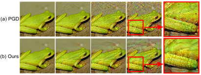
Figure 1: Comparison between the targeted adversarial example generated by the normal PGD attack and our distribution-relevant attack. We set the maximum allowable adversarial perturbation as $\epsilon$ = 32/255 with respect to a pixel value in [0, 1] for visibility. The leftmost column of each figure shows the original image (tree frog), while the other column shows the adversarial images (target class: corn) under different attack strengths. The rightmost column amplifies the square patch in the adversarial examples.

Towards this end, we propose a method named Distribution-Relevant Attack (DRA) to demonstrate our hypothesis. We attempt to push the input image away from its original distribution to generate transferable adversarial examples. However, as we do not have access to the ground truth data distribution, it is technically challenging to push the images away from its original distribution directly.

We borrow the idea from the score-matching generative models [25, 26, 27, 28], which propose to estimate the gradient of the ground truth data distribution $\nabla_{\boldsymbol{x}}\log p_{D}(\boldsymbol{x}|y)$ and generate the image of the certain distribution iteratively using the estimated gradient of the ground truth data distribution through Langevin dynamics [25, 27]. Previous attacks iteratively minimize (maximize) the conditional density of the model $p_{\theta}(y|\boldsymbol{x})$ along the gradient of the conditional density of the model $\nabla_{\boldsymbol{x}}\log p_{\theta}(y|\boldsymbol{x})$ to perform the untargeted (targeted) attacks. Thus, to estimate the gradient of the ground truth data distribution in the transfer attack scenarios, we fine-tune the surrogate classifier to match the gradient of the conditional density of the model and the gradient of ground truth data distribution. Thereby, the gradient of the fine-tuned model can approximate the gradient of the ground truth data distribution and the process of generating the adversarial examples with the gradient of our fine-tuned models can approximate the process of the Langevin dynamics, which enables us to manipulate the distribution of the image. We name the attack that uses our fine-tuned models to push the image away from the original distribution while generating the adversarial examples Distribution-Relevant Attack (DRA). What’s more, DRA is compatible with existing transfer attacks and can greatly improve the performance of these attacks.

Visually, targeted adversarial perturbation generated by our method, which can drag the image into the target distribution, reflects vivid semantic features of the target class (See Fig.1: Turning the tree frog to corn). In Fig.2, we use the out-of-distribution (OOD) detection method Energy [29] to evaluate that our DRA can indeed move the image out of its original distribution, performing better than the normal PGD attack.

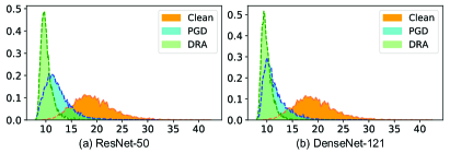
Figure 2: The distribution of the Energy OOD scores [29] for the in-distribution images (ImageNet) and the untargeted adversarial examples generated by the original PGD attack and our DRA on ResNet-50 (a) and DenseNet-121 (b). Examples with lower OOD scores than the clean images are regarded as the out-of-distribution (OOD) examples and examples with higher energy scores are regarded as the in-distribution (ID) examples.

We have conducted extensive evaluations and established state-of-the-art performance in both untargeted and targeted attack scenarios, improving the targeted attack success rate by up to 40$\%$ in some cases. This work provides new insight into the understanding of adversarial transferability from a data distribution perspective and provides a strong counterpart for future research on defense.

The main contributions of our paper are summarized as follows:

• We provide a new understanding of adversarial transferability from the perspective of data distribution, advocating that adversarial transferability can be enhanced by pushing the images away from its original distribution.

• We introduce a method to match the gradient of the model and the gradient of the data distribution, which enables us to push the image away from its original distribution using the gradient of the model.

• Extensive experiments demonstrate that our DRA outperforms state-of-the-art approaches a lot in both untargeted and targeted attack scenarios (even up to 40% in most cases).

The rest of the paper is organized as follows. Section II summarizes the literature related to adversarial attacks. In Section III, we firstly present some preliminaries and the motivation of our method. Then we introduce the optimization of the distance between the gradient of the model and the gradient of the data distribution. After that, we propose the Algorithm of our DRA, which fine-tunes the original surrogate model and use the fine-tuned model to generate adversarial examples. In Section IV, we firstly conduct untargeted transfer attack experiments to demonstrate the superiority of DRA against various target models, including both normal models and secured models. Then, we evaluate the effectiveness of DRA in the targeted attack scenario which is more difficult than the untargeted scenario. Section V provides some discussion to further understand our method. Section VI gives some conclusive results.

II Related Work

In this section, we briefly review the literature related to adversarial attacks.

Deep neural networks (DNNs) obtained by normal training are vulnerable to adversarial examples [10]. This phenomenon has drawn wide concern and affected the deployment of DNNs in many safety-critical fields, such as face recognition [30, 31, 32], medical diagnosis [33, 34], speaker recognition [35, 36], and autonomous driving [37, 38]. According to the access rights to the target model, adversarial attacks can be classified as white-box attacks and black-box attacks.

White-box attacks assume that the attacker can completely access the structure and parameters of the target model. Typical examples of white-box attacks are FGSM [11], BIM [39], PGD [40], DeepFool [41], JSM [42], and CW [43]. The widely used PGD attack builds an adversarial example by performing multi-step gradient updating along the direction of the gradient at each pixel and projecting the perturbation into the specified range.

Black-box attacks assume that the attacker only knows the output of the target model (prediction or confidence), including query-based attacks and transfer attacks. Query-based attacks perform the black-box attack by estimating gradient with queries to the target model [44, 45, 46, 47]. In this paper, we assume that the attacker can only generate adversarial perturbation using a surrogate model without any queries on the target model. This method is much more efficient and is relatively harder to detect by the target system than query-based attacks. Thus, many existing works focused on leveraging the transferability of adversarial examples.

Iterative Methods:  Liu et al. [12] show that adversarial attacks can be transferred between different models. Iterative methods attack a surrogate model and update the perturbation iteratively using gradient information [48, 17, 18, 49, 13, 50, 51, 52]. The iterative attack methods such as BIM [39] and PGD [40] could achieve good performance in white-box attack scenarios, but they often suffer from low transferability. Recently, many methods have been proposed to improve the adversarial transferability of the iterative methods.

Some methods suggest stabilizing update directions for the iterative algorithms.  Dong et al. [48] propose to improve the adversarial transferability by integrating the momentum of gradients into the update of perturbation. Lin et al. [18] adapt Nesterov accelerated gradient into the update of perturbation to enhance the adversarial transferability. Data augmentation, which plays an important role in improving model generalization and mitigating over-fitting, also contributes to adversarial transferability. Xie et al. [17] suggest applying random transformations (resizing and padding) to the input images at each iteration during attacking. Lin et al. [18] take the scale copies of the input images into attack in order to mitigate overfitting on the surrogate model. Wang et al. [19] propose Admix, which attacks the input image admixed with a group of images randomly sampled from other categories. Wang et al. [50] propose a loss to decrease interactions between perturbation units during attacking. There are also some model-specific methods to improve adversarial transferability.  Huang et al. [22] fine-tune the adversarial examples by increasing perturbation on a pre-specified layer. Wu et al. [13] propose to reduce the gradients from the residual modules and pay attention to the architectural vulnerability of DNNs. Guo et al. [51] show that properly increasing the linearity of DNNs can enhance adversarial transferability.

These methods perform well in untargeted attacks, but their performance degrades severely in targeted attacks.

Generative Methods: The methods generating the targeted adversarial perturbations by generative models always perform better than iterative methods at the expense of training the same number of generative models as the labels [53, 54, 55, 20, 21]. Poursaeed et al. [54] propose to train the generative model against the surrogate classifier via cross-entropy loss. Naseer et al. [20] show that the relativistic cross-entropy loss can improve the performance of the generative model. Naseer et al. [21] propose to match the ‘distribution’ of perturbed images with that of the target class within latent space of the surrogate classifier in generative training so as to reduce the reliance on class-boundary information from the surrogate classifier. This method can successfully imprint the features of the target distribution to the image and achieves satisfactory targeted attack performance but needs to train generators for every class which is nontrivial on large-scale datasets.

Compared with the existing iterative methods, our DRA pays attention to the distribution-relevant information in the surrogate model rather than improving the iterative algorithm or performing data augmentation. DRA overcomes the low transferability of iterative attacks in targeted attack scenarios. The generative methods aim to learn the distribution of the adversarial perturbation, while our DRA focuses on the ground truth distribution. As we show in our experiments, our DRA greatly improves the adversarial transferability and surpasses existing methods in both untargeted and targeted scenarios.

III Method

III-A Preliminary

Given a surrogate classifier $f_{\theta}$ parameterized by $\theta$, and image $\boldsymbol{x}$, label $y$, total possible classes $n$, then $f_{\theta}(\boldsymbol{x})[k]$ represents the $k^{th}$ output of the last layer.

The conditional density $p_{\theta}(y|{\boldsymbol{x}})$ can be expressed as:

$$p_{\theta}(y|\boldsymbol{x})=\frac{\exp({f_{\theta}(\boldsymbol{x})[y]})}{\sum_{k=1}^{n}\exp({f_{\theta}(\boldsymbol{x})[k]})}.$$ (1)

The adversarial perturbation is usually based on the gradient of the classification loss $\mathcal{L}$. The untargeted attack aims to minimize the conditional density $p_{\theta}(y|\boldsymbol{x})$ and can be expressed as [11, 40]:

$$\boldsymbol{x}^{\prime}=\boldsymbol{x}+\nabla_{\boldsymbol{x}}\mathcal{L}(f_{\theta}(\boldsymbol{x}),y)=\boldsymbol{x}-\nabla_{\boldsymbol{\boldsymbol{x}}}\log p_{\theta}(y|\boldsymbol{x}),$$ (2)

where $\boldsymbol{x}^{\prime}$ means the adversarial example of the image $\boldsymbol{x}$. The targeted attack aims to maximize the conditional density $p_{\theta}(y_{target}|\boldsymbol{x})$ and can be expressed as:

$$\boldsymbol{x}^{\prime}=\boldsymbol{x}-\nabla_{\boldsymbol{x}}\mathcal{L}(f_{\theta}(\boldsymbol{x}),y_{target})=\boldsymbol{x}+\nabla_{\boldsymbol{\boldsymbol{x}}}\log p_{\theta}(y_{target}|\boldsymbol{x}).$$ (3)

The goal of the transfer attack is to mislead the target model using the adversarial examples generated by the surrogate model.

III-B Motivation

The existing transfer attacks iteratively minimize $p_{\theta}(y_{label}|\boldsymbol{x})$ (untargeted attack) or maximize $p_{\theta}(y_{target}|\boldsymbol{x})$ (targeted attack) of the surrogate model to generate adversarial examples and then use these adversarial examples to attack the target models. However, the existing transfer attacks can hardly perform targeted attacks successfully and lack the explanation why minimizing $p_{\theta}(y|\boldsymbol{x})$ of the surrogate model can also fool the target model with different model parameters and architectures from the surrogate model.

In this paper, we propose to understand and improve the adversarial transferability from a data distribution perspective, which builds on the classical assumption in machine learning methods [23, 24] that the deep models can properly classify the validation data that is independent and identically distributed with the training dataset but can hardly classify the out-of-distribution examples. Specifically, the models tend to predict the label of the image that is identically distributed with $p_{D}(\boldsymbol{x}|y)$ as $y$, but can not handle the out of distribution images properly. We hypothesize that moving the image out of its original distribution can achieve high untargeted adversarial transferability and dragging the image into the target distribution $p_{D}(\boldsymbol{x}|y_{target})$ can achieve high targeted adversarial transferability. The challenge comes from how to push the image away from its original distribution as we don’t have access to the ground truth class-conditional data distribution $p_{D}(\boldsymbol{x}|y)$.

We borrow the idea from the score-matching generative models [25, 26, 27] which propose to estimate the gradient of the ground truth data distribution and then move the initial image from its original distribution $p_{D}(\boldsymbol{x}|y_{0})$ to the target distribution $p_{D}(\boldsymbol{x}|y)$ iteratively through the Stochastic Gradient Langevin Dynamics (SGLD) [28, 56, 57]:

$$\boldsymbol{x}_{t}=\boldsymbol{x}_{t-1}+\alpha\cdot\nabla_{\boldsymbol{x}_{t-1}}\log p_{D}(\boldsymbol{x}_{t-1}|y)+\sqrt{2\alpha}\cdot\epsilon.$$ (4)

The $\epsilon\sim\mathcal{N}(0,I)$ and $\alpha$ is a fixed step size. When $\alpha\rightarrow 0$ and $T\rightarrow\infty$, $\boldsymbol{x}_{T}$ is exactly an sample from $p_{D}(\boldsymbol{x}|y)$. Updating the SGLD process along the opposite direction of $\nabla_{\boldsymbol{x}}\log p_{D}(\boldsymbol{x}|y)$ can move the image away from the distribution $p_{D}(\boldsymbol{x}|y)$. Based on the above reasoning, the gradient of the data distribution can be used to manipulate the distribution of the input via iterative methods.

In this paper, we propose to match the gradient of the log conditional density $\nabla_{\boldsymbol{x}}\log p_{\theta}(y|\boldsymbol{x})$ (the direction of the normal adversarial attack) and the gradient of the log ground truth class-conditional data distribution $\nabla_{\boldsymbol{x}}\log p_{D}(\boldsymbol{x}|y)$. In this way, the adversarial attack can approximate the direction of the gradient of the ground truth class-conditional data distribution.

To be specific, if $\nabla_{\boldsymbol{x}}\log p_{\theta}(y|\boldsymbol{x})$ matches $\nabla_{\boldsymbol{x}}\log p_{D}(\boldsymbol{x}|y)$ well, the untargeted attack $x^{\prime}=x-\eta\cdot\nabla_{\boldsymbol{\boldsymbol{x}}}\log p_{\theta}(y_{label}|\boldsymbol{x})$ can be regarded as an approximation of the opposite process of SGLD sampling $\boldsymbol{x}_{t}=\boldsymbol{x}_{t-1}-\alpha\cdot\nabla_{\boldsymbol{x}_{t-1}}\log p_{D}(\boldsymbol{x}_{t-1}|y_{label})$, which moves the images out of its original distribution $p_{D}(\boldsymbol{x}|y_{label})$. Fig.2 shows that our untargeted attack indeed moves the image out of its original distribution, which causes difficulties for different models to classify this image.

Similarly, if $\nabla_{\boldsymbol{x}}\log p_{\theta}(y|\boldsymbol{x})$ matches $\nabla_{\boldsymbol{x}}\log p_{D}(\boldsymbol{x}|y)$ well, our targeted attack $x^{\prime}=x+\eta\cdot\nabla_{\boldsymbol{\boldsymbol{x}}}\log p_{\theta}(y_{target}|\boldsymbol{x})$ can be regarded as an approximation of the process of SGLD sampling $\boldsymbol{x}_{t}=\boldsymbol{x}_{t-1}+\alpha\cdot\nabla_{\boldsymbol{x}_{t-1}}\log p_{D}(\boldsymbol{x}_{t-1}|y_{target})$, which drags the image to the target distribution $p_{D}(\boldsymbol{x}|y_{target})$. Fig.1 shows that our method can imprint the features of the target distribution to the image and semantically change the tree-frog to corn, which can mislead the models to classify the image as the target class. Compared with the existing transfer attacks, our method aims to intrinsically manipulate the distribution of the image rather than just minimizing or maximizing the classification loss.

In the next subsection, we provide an appealingly simple and generic technique to match the $\nabla_{\boldsymbol{x}}\log p_{\theta}(y|\boldsymbol{x})$ and $\nabla_{\boldsymbol{x}}\log p_{D}(\boldsymbol{x}|y)$. The last subsection instructs how to generate high transferable adversarial examples with our method.

III-C Decreasing the Distance Between Gradients

In this section, we propose a novel method to decrease the distance between the gradients, which enables us to use the gradient of the model to estimate the gradient of the ground truth data distribution. In this way, adversarial attack can push the image away from its original distribution through Langevin Dynamics (Eq.(4)).

We define the Distance between the gradient of log Conditional density and the gradient of log Ground truth class-conditional data distribution (DCG) as :

$$\mathop{\rm{DCG}}\triangleq{\mathbb{E}_{p_{D}(y)}}\mathbb{E}_{p_{D}(\boldsymbol{x}|y)}\|\nabla_{\boldsymbol{x}}\log p_{\theta}(y|\boldsymbol{x})-\nabla_{\boldsymbol{x}}\log p_{D}({\boldsymbol{x}}|y)\|_{2}^{2}$$ (5)

$$=\int\int\|\nabla_{\boldsymbol{x}}\log p_{\theta}(y|\boldsymbol{x})-\nabla_{\boldsymbol{x}}\log p_{D}({\boldsymbol{x}}|y)\|_{2}^{2}p_{D}(\boldsymbol{x}|y)p_{D}(y)d\boldsymbol{x}dy$$

$$=\int\int\|\nabla_{\boldsymbol{x}}\log p_{D}({\boldsymbol{x}}|y)\|_{2}^{2}p_{D}(\boldsymbol{x}|y)p_{D}(y)d\boldsymbol{x}dy$$

$$+\int\int\|\nabla_{\boldsymbol{x}}\log p_{\theta}(y|\boldsymbol{x})\|_{2}^{2}p_{D}(\boldsymbol{x}|y)p_{D}(y)d\boldsymbol{x}dy$$

$$-2\int\int(\nabla_{\boldsymbol{x}}\log p_{\theta}(y|\boldsymbol{x})^{\rm{T}}\cdot\nabla_{\boldsymbol{x}}\log p_{D}({\boldsymbol{x}}|y))p_{D}(\boldsymbol{x}|y)p_{D}(y)d\boldsymbol{x}dy.$$

We omit the integration domain here for simplicity. The first term is a constant which does not depend on the model’s parameters $\theta$. The middle term can be expressed as $\mathbb{E}_{p_{D}(y)}\mathbb{E}_{p_{D}(\boldsymbol{x}|y)}\left\|\nabla_{\boldsymbol{x}}\log p_{\theta}(y|\boldsymbol{x})\right\|_{2}^{2}$ is tractable since this term does not contain the unknown score of the ground truth distribution. The last term is not directly computable, because the score of the ground truth distribution $\nabla_{\boldsymbol{x}}\log p_{D}({\boldsymbol{x}}|y)$ is unknown. Score matching methods [26, 27, 58] eliminate the score of the ground truth distribution using integration by parts. Inspired by these methods, we apply integration by parts to the last term in Eq.(5) as:

$$\int_{-\infty}^{+\infty}p_{D}(y)dy\int_{\boldsymbol{x}\in\mathbb{R}^{n}}(\nabla_{\boldsymbol{x}}\log p_{\theta}(y|\boldsymbol{x})^{\rm{T}}\cdot\nabla_{\boldsymbol{x}}\log p_{D}({\boldsymbol{x}}|y))p_{D}(\boldsymbol{x}|y)d\boldsymbol{x}$$ (6)

$$\overset{\text{(I)}}{=}\int_{-\infty}^{+\infty}p_{D}(y)dy\int_{\boldsymbol{x}\in\mathbb{R}^{n}}(\nabla_{\boldsymbol{x}}\log p_{\theta}(y|\boldsymbol{x})^{\rm{T}}\cdot\nabla_{\boldsymbol{x}}p_{D}({\boldsymbol{x}}|y))d\boldsymbol{x}$$

$$\overset{\text{(II)}}{=}\int_{-\infty}^{+\infty}p_{D}(y)dy\sum_{i=1}^{n}\int_{\boldsymbol{x}\in\mathbb{R}^{n}}\nabla_{{x_{i}}}\log p_{\theta}(y|\boldsymbol{x})\nabla_{{x_{i}}}p_{D}({\boldsymbol{x}}|y)d{\boldsymbol{x}}$$

$$\overset{\text{(III)}}{=}\int_{-\infty}^{+\infty}p_{D}(y)dy\sum_{i=1}^{n}\int_{\tilde{\boldsymbol{x}}_{i}\in\mathbb{R}^{n-1}}[\lim_{M\to\infty}p_{D}(\boldsymbol{x}|y)\nabla_{x_{i}}\log p_{\theta}(y|\boldsymbol{x})|_{-\boldsymbol{M}_{i}}^{+\boldsymbol{M}_{i}}]d{\tilde{\boldsymbol{x}}_{i}}$$

$$\quad-\int_{-\infty}^{+\infty}p_{D}(y)dy\sum_{i=1}^{n}\int_{\tilde{\boldsymbol{x}}_{i}\in\mathbb{R}^{n-1}}[\int_{-\infty}^{+\infty}p_{D}(\boldsymbol{x}|y)\nabla^{2}_{x_{i}}\log p_{\theta}(y|\boldsymbol{x})d{x_{i}}]d{\tilde{\boldsymbol{x}}_{i}}$$

$$\overset{\text{(IV)}}{=}-\mathbb{E}_{p_{D}(y)}\mathbb{E}_{p_{D}({\boldsymbol{x}}|y)}\left[{\rm{tr}}(\nabla^{2}_{\boldsymbol{x}}\log p_{\theta}(y|{\boldsymbol{x}}))\right],$$

where $\nabla^{2}_{\boldsymbol{x}}$ denotes the Hessian with respect to $\boldsymbol{x}$. “+$\boldsymbol{M}_{i}$” represents the vector $[x_{1},...,x_{i-1},+M,x_{i+1},...,x_{n}]$. “-$\boldsymbol{M}_{i}$” represents the vector $[x_{1},...,x_{i-1},-M,x_{i+1},...,x_{n}]$. $\boldsymbol{x}=[x_{1},...,x_{n}]$ is an n-dimensional vector. $\tilde{\boldsymbol{x}}_{i}=[x_{1},...,x_{i-1},x_{i+1},...,x_{n}]$. See Appendix for detailed derivation.

We use the formula: $\nabla_{x}\log f(x)=f(x)^{-1}\nabla_{x}f(x)$ for equality (I). In equality (I), $\nabla_{\boldsymbol{x}}\log p_{\theta}(y|\boldsymbol{x})^{\rm{T}}$ and $\nabla_{\boldsymbol{x}}\log p_{D}({\boldsymbol{x}}|y)$ are n-dimensional vectors, and their product result is a scalar. We use the formula: $\boldsymbol{u}^{T}\cdot\boldsymbol{v}=\sum_{i=1}^{n}u_{i}v_{i}$ for equality (II), where n represents the dimension of the data. As for equality (III), we use the integration by parts formula (See Appendix for proof):

$$\int_{-\infty}^{+\infty}\nabla_{{x_{i}}}f(\boldsymbol{x})\nabla_{{x_{i}}}g(\boldsymbol{x})d{x_{i}} =\lim_{M\to\infty}g({\boldsymbol{x}})\nabla_{{x_{i}}}f({\boldsymbol{x}})|_{-\boldsymbol{M}_{i}}^{+\boldsymbol{M}_{i}}$$ (7)

$$-\int_{-\infty}^{+\infty}g(\boldsymbol{x})\nabla_{{x_{i}}}^{2}f(\boldsymbol{x})dx_{i}.$$

The equality (IV) holds for that we assume $p_{D}({\boldsymbol{x}}|y)\rightarrow 0$ when $||\boldsymbol{x}||_{2}\rightarrow\infty$.

Thus, substituting the results of integration by parts into Eq.(5), the DCG loss can be reformulated as:

$$\mathop{\rm{DCG}} \triangleq\mathbb{E}_{p_{D}(y)}\mathbb{E}_{p_{D}(\boldsymbol{x}|y)}\|\nabla_{\boldsymbol{x}}\log p_{\theta}(y|\boldsymbol{x})-\nabla_{\boldsymbol{x}}\log p_{D}({\boldsymbol{x}}|y)\|_{2}^{2}$$ (8)

$$=\mathbb{E}_{p_{D}(y)}\mathbb{E}_{p_{D}(\boldsymbol{x}|y)}\left\|\nabla_{\boldsymbol{x}}\log p_{\theta}(y|\boldsymbol{x})\right\|_{2}^{2}$$

$$+2\cdot\mathbb{E}_{p_{D}(y)}\mathbb{E}_{p_{D}(\boldsymbol{x}|y)}[{\rm{tr}}(\nabla_{\boldsymbol{x}}^{2}\log p_{\theta}(y|\boldsymbol{x}))]+{\rm const}.$$

We ignore the const in Eq.(8) that does not depend on the model parameters and denote the DCG loss as $\mathcal{L}_{\rm{DCG}}$:

$$\mathop{\mathcal{L}_{\rm DCG}} \triangleq\mathbb{E}_{p_{D}(y)}\mathbb{E}_{p_{D}(\boldsymbol{x}|y)}\left\|\nabla_{\boldsymbol{x}}\log p_{\theta}(y|\boldsymbol{x})\right\|_{2}^{2}$$ (9)

$$+2\cdot\mathbb{E}_{p_{D}(y)}\mathbb{E}_{p_{D}(\boldsymbol{x}|y)}[{\rm{tr}}(\nabla_{\boldsymbol{x}}^{2}\log p_{\theta}(y|\boldsymbol{x}))].$$

Computing the Hessian trace term in Eq.9 requires a number of backpropagations that is proportional to the data dimension, which is intractable for high-dimensional data. Hutchinson’s trick [59] is a stochastic algorithm to approximate tr($\boldsymbol{A}$) for any square matrix $\boldsymbol{A}$. For a distribution of a random vector $\boldsymbol{v}$ such that $\mathbb{E}_{p(\boldsymbol{v})}[\boldsymbol{v}\boldsymbol{v}^{\mathrm{T}}]=I$, Hutchinson’s trick approximate tr($\boldsymbol{A}$) as : ${\rm{tr}}(\boldsymbol{A})=\mathbb{E}_{p(\boldsymbol{v})}[\boldsymbol{v}^{\mathrm{T}}\boldsymbol{A}\boldsymbol{v}]$. Hence, using Hutchinson’s trick, we can replace ${\rm{tr}}(\nabla_{\boldsymbol{x}}^{2}\log p_{\theta}(y|\boldsymbol{x}))$ with $\mathbb{E}_{p(\boldsymbol{v})}[\boldsymbol{v}^{\mathrm{T}}\nabla_{\boldsymbol{x}}^{2}\log p_{\theta}(y|\boldsymbol{x})\boldsymbol{v}]$. Thus we can reformulate the $\mathcal{L}_{\rm{DCG}}$ as:

$$\mathop{\mathcal{L}_{\rm DCG}} \triangleq\mathbb{E}_{p_{D}(y)}\mathbb{E}_{p_{D}(\boldsymbol{x}|y)}\left\|\nabla_{\boldsymbol{x}}\log p_{\theta}(y|\boldsymbol{x})\right\|_{2}^{2}$$ (10)

$$+2\cdot\mathbb{E}_{p_{D}(y)}\mathbb{E}_{p_{D}(\boldsymbol{x}|y)}\mathbb{E}_{p(\boldsymbol{v})}[\boldsymbol{v}^{\mathrm{T}}\nabla_{\boldsymbol{x}}^{2}\log p_{\theta}(y|\boldsymbol{x})\boldsymbol{v}].$$

In practice, we can tune the number of samples $\boldsymbol{v}$ to trade off the performance of estimation and computational cost. With reference to the existing methods [25, 26], we sample one random vector $\boldsymbol{v}$ independently for each input during the training process. The first term in Eq.(10) can be computed by one backpropagation. The second term involves Hessian, but it is in the form of Hessian-vector products, which can be computed within $O(1)$ backpropagations. Therefore, the computation of Eq.(10) does not depend on the dimension of data and is scalable for training deep models on high-dimensional datasets.

We propose fine-tuning the surrogate model by optimizing the classification loss and the DCG loss jointly during training. The optimization objective can be formulated as:

$$\mathop{minimize}\limits_{\theta}\ [\mathcal{L}(f_{\theta}(x),y)+\lambda\;\mathcal{L}_{\rm DCG}],$$ (11)

where $\lambda$ represents the regularization strength.

In this way, we can obtain a fine-tuned surrogate model whose gradient of log conditional density $\nabla_{\boldsymbol{\boldsymbol{x}}}\log p_{\theta}(y|\boldsymbol{x})$ aligns with the gradient of log ground truth class-conditional data distribution $\nabla_{\boldsymbol{x}}\log p_{D}(\boldsymbol{x}|y)$ better than the original surrogate model. Moreover, we can manipulate the distribution information of the image through the iterative adversarial attack with the fine-tuned model.

III-D Distribution-Relevant Attack

We named the attack using our distribution-relevant fine-tuned surrogate models as Distribution-Relevant Attack (DRA). DRA consists of two steps: fine-tuning the surrogate model to decrease the distance between the gradient of the model and the gradient of the ground truth data distribution, and using the fine-tuned surrogate model to generate adversarial perturbation with the guidance of the approximate gradient of the ground truth distribution. Alg. 1 details our method.

We jointly optimize the DCG loss $\mathcal{L}_{\rm{DCG}}$ and the classification loss $\mathcal{L}$ to fine-tune the surrogate model. This optimization process encourages the direction of the gradient of the surrogate model to match the direction of the gradient of the ground truth data distribution.

Our proposed fine-tuned method aims to enable the attackers to push the image away from its original distribution using the gradient of the model. With the fine-tuned surrogate model, we can use most existing transfer attack methods to conduct attacks. We mainly choose the widely used iterative attack method, projected gradient descent (PGD) [39, 40] to generate adversarial examples. Our fine-tuning method is also compatible with other advanced transfer attacks.

III-D1 Untargeted attack

The untargeted attack can be formulated as:

$$\left\{\begin{array}[]{l}\boldsymbol{x_{n}}=\boldsymbol{x_{n-1}}+\eta\cdot sign(\nabla_{\boldsymbol{x_{n-1}}}\mathcal{L}(f_{\theta}(\boldsymbol{x_{n-1}}),y_{label}),\\ \boldsymbol{x_{n}}=clip(\boldsymbol{x_{n}},\boldsymbol{x_{0}}-\epsilon,\boldsymbol{x_{0}}+\epsilon),\end{array}\right.$$ (12)

where $x_{n}$ is the generated adversarial example after $n$ steps, and $x_{0}$ is the clean image. $\mathcal{L}$ is the classification loss, $\eta$ is the perturbation step size, and $y_{label}$ is the original label for the clean image. The $clip$ operation aims to make the perturbation bounded in the budget $\epsilon$.

Algorithm 1 Distribution-Relevant Attack DRA: Given network $f_{\theta}$ parameterized by $\theta$, regularization constant $\lambda$, epochs $T$, total batches $M$, learning rate $\eta$, the classification loss $\mathcal{L}$, the DCG loss $\mathcal{L}_{{\rm DCG}}$. Adversarial perturbation $\boldsymbol{\delta}$, original image $\boldsymbol{x}$, $\ell_{\infty}$ perturbation radius $\epsilon$; step size $\alpha$; iterations $N$.

  $\blacktriangleright$ Fine-tuning:

  for $i=1,2...,T$ do

     for $j=1,2...,M$ do

        Updating model parameters:

        $\theta=\theta-\eta\cdot(\nabla_{\theta}\mathcal{L}(f_{\theta}(x_{j}),y_{j})+\lambda\cdot\nabla_{\theta}\mathcal{L}_{\rm DCG})$

     end for

  end for

  return Fine-tuned network $f_{\theta}$

  

  $\blacktriangleright$ Untargeted Attack:

  Initialize ${\boldsymbol{\delta}}=Uniform(-\epsilon,\epsilon)$.

  for $i=1,2,...,N$ do

     $\boldsymbol{\delta}=\boldsymbol{\delta}+\alpha\cdot sign(\nabla_{\boldsymbol{x}}\mathcal{L}(f_{\theta}({\boldsymbol{x}+\boldsymbol{\delta}}),y_{label})$,

     $\boldsymbol{\delta}=max(min(\boldsymbol{\delta},\epsilon),-\epsilon)$

  end for

  return $\boldsymbol{\delta}$

  

  $\blacktriangleright$ Targeted Attack:

  Initialize ${\boldsymbol{\delta}}=Uniform(-\epsilon,\epsilon)$.

  for $i=1,2,...,N$ do

     $\boldsymbol{\delta}=\boldsymbol{\delta}-\alpha\cdot sign(\nabla_{\boldsymbol{x}}\mathcal{L}(f_{\theta}({\boldsymbol{x}+\boldsymbol{\delta}}),y_{target})$,

     $\boldsymbol{\delta}=max(min(\boldsymbol{\delta},\epsilon),-\epsilon)$

  end for

  return $\boldsymbol{\delta}$

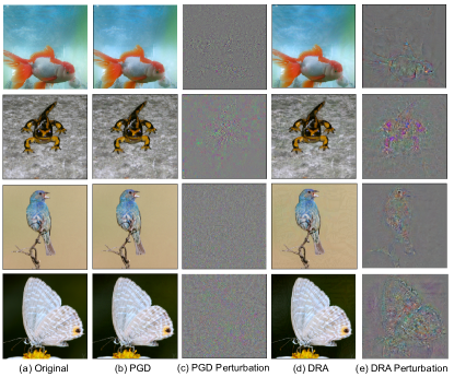
Figure 3: Comparison between the untargeted adversarial examples generated by PGD attack and our DRA. (a) The original images. (b) The adversarial examples generated by the PGD attack. (c) Normalizing the PGD perturbation to [0,1] for visibility. (d) The adversarial examples generated by DRA. (e) Normalizing the DRA perturbation to [0,1]. These adversarial examples are projected within a small distance (e.g., $\ell_{\infty}$ $\epsilon\leq 16/255$) during inference.

Although DRA and other iterative methods are similar in expression when generating untargeted attacks, the direction of the DRA attack is better aligned with the gradient of the data distribution. In other words, DRA moves the image out of its original distribution to generate untargeted attacks, while the other iterative methods pay attention to dragging the inputs across the decision boundary of the classifier. As shown in Fig.2, the adversarial examples generated by our DRA are regarded as the out-of-distribution examples. Fig.3 shows the difference between the adversarial examples generated by DRA and PGD. The adversarial perturbation of the untargeted attack generated by DRA concentrates on the semantic features of the image while the adversarial perturbation generated by the PGD attack seems irregular.

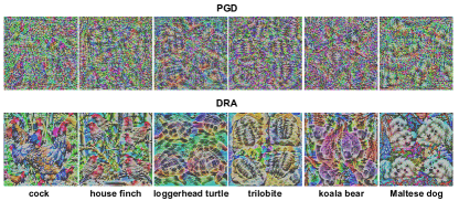
Figure 4: The targeted perturbation (unbounded perturbation for visibility) generated from the mean image. The perturbation generated by our DRA can reflect the semantic features of the target category while the perturbation generated by the PGD attack seems more noisy.

III-D2 Targeted attack

Similar to the untargeted DRA, the targeted version of DRA can be formulated as:

$$\left\{\begin{array}[]{l}\boldsymbol{x_{n}}=\boldsymbol{x_{n-1}}-\eta\cdot sign(\nabla_{\boldsymbol{x_{n-1}}}\mathcal{L}(f_{\theta}(\boldsymbol{x_{n-1}}),y_{target}),\\ \boldsymbol{x_{n}}=clip(\boldsymbol{x_{n}},\boldsymbol{x_{0}}-\epsilon,\boldsymbol{x_{0}}+\epsilon),\end{array}\right.$$ (13)

where attackers aim to make the DNNs misclassify the input as the target class $y_{target}$. We generate the targeted attack starting from the mean image and show the perturbation in Fig. 4. The perturbation generated by DRA represents recognizable features of the target distribution, while the perturbation generated by the PGD attack does not show obvious features. The targeted adversarial perturbation, which contains the sufficient features of the target category, may dominate the classification and the original features act like noise with respect to perturbations.

Compared with the prior research on adversarial transferability by improving the attack optimization procedure, we focus on the ground truth data distribution and match the gradient of the surrogate model to the gradient of the data distribution. We use the fine-tuned surrogate model to generate the iterative attack. In the following section, we try to validate the effectiveness of the proposed DRA in both untargeted and targeted attack scenarios quantitatively.

IV Experiment

TABLE I: Transferability against normal models: the success rates of black-box attacks (untargeted) crafted on RN50, RN152, DN121 and DN201. The maximum standard deviation of this experiment is 0.92$\%$ which is much less than our improvement. The best results are in bold.

Model	Attack	VGG19	RN152	DN121	DN201	SE154	IncV3	IncV4	IncRes	ViT
RN50	PGD [40]	53.00$\%$	61.26$\%$	55.62$\%$	53.56$\%$	24.78$\%$	20.86$\%$	21.96$\%$	17.60$\%$	3.82$\%$
	DI [17]	75.06$\%$	81.65$\%$	81.98$\%$	74.80$\%$	52.42$\%$	42.58$\%$	44.30$\%$	27.12$\%$	7.12$\%$
	MI [48]	64.86$\%$	73.22$\%$	73.50$\%$	64.33$\%$	47.20$\%$	39.08$\%$	37.35$\%$	25.26$\%$	13.34$\%$
	ILA [22]	83.56$\%$	92.46$\%$	88.40$\%$	85.24$\%$	61.44$\%$	49.94$\%$	48.34$\%$	35.74$\%$	11.26$\%$
	SGM [13]	82.72$\%$	88.40$\%$	83.56$\%$	80.34$\%$	61.30$\%$	53.72$\%$	49.83$\%$	42.86$\%$	18.82$\%$
	IR [50]	82.46$\%$	85.24$\%$	84.35$\%$	82.10$\%$	64.20$\%$	54.60$\%$	51.05$\%$	46.78$\%$	17.76$\%$
	DRA+PGD	98.26$\%$	99.24$\%$	99.56$\%$	99.28$\%$	93.92$\%$	95.56$\%$	92.66$\%$	92.56$\%$	58.46$\%$
Model	Attack	VGG19	RN50	DN121	DN201	SE154	IncV3	IncV4	IncRes	ViT
RN152	PGD [40]	49.32$\%$	72.72$\%$	53.44$\%$	51.00$\%$	26.32$\%$	23.50$\%$	22.58$\%$	18.72$\%$	5.10$\%$
	DI [17]	74.01$\%$	88.18$\%$	79.46$\%$	77.81$\%$	57.49$\%$	50.28$\%$	47.16$\%$	35.10$\%$	10.40$\%$
	MI [48]	65.42$\%$	83.40$\%$	77.60$\%$	75.79$\%$	53.00$\%$	46.50$\%$	43.32$\%$	33.08$\%$	15.28$\%$
	ILA [22]	66.20$\%$	90.44$\%$	75.48$\%$	73.80$\%$	50.32$\%$	42.32$\%$	41.30$\%$	29.98$\%$	12.26$\%$
	SGM [13]	80.40$\%$	96.10$\%$	85.80$\%$	82.76$\%$	61.90$\%$	53.16$\%$	49.24$\%$	43.30$\%$	11.72$\%$
	IR [50]	73.20$\%$	92.70$\%$	83.43$\%$	80.60$\%$	64.00$\%$	53.60$\%$	50.30$\%$	48.00$\%$	10.24$\%$
	DRA+PGD	96.36$\%$	99.62$\%$	99.28$\%$	98.92$\%$	92.98$\%$	95.00$\%$	91.00$\%$	91.52$\%$	52.08$\%$
Model	Attack	VGG19	RN50	RN152	DN201	SE154	IncV3	IncV4	IncRes	ViT
DN121	PGD [40]	56.78$\%$	63.22$\%$	52.76$\%$	71.98$\%$	31.46$\%$	24.92$\%$	26.82$\%$	20.64$\%$	4.62$\%$
	DI [17]	73.68$\%$	79.56$\%$	74.72$\%$	89.40$\%$	53.34$\%$	53.65$\%$	47.94$\%$	37.72$\%$	7.54$\%$
	MI [48]	68.36$\%$	74.18$\%$	72.88$\%$	89.56$\%$	58.58$\%$	52.22$\%$	45.35$\%$	35.24$\%$	14.84$\%$
	ILA [22]	87.76$\%$	90.38$\%$	83.42$\%$	95.32$\%$	65.02$\%$	58.64$\%$	57.36$\%$	40.76$\%$	9.60$\%$
	SGM [13]	80.18$\%$	88.54$\%$	80.54$\%$	92.70$\%$	64.92$\%$	54.62$\%$	49.82$\%$	37.76$\%$	12.80$\%$
	IR [50]	82.56$\%$	86.14$\%$	85.20$\%$	95.30$\%$	72.20$\%$	62.22$\%$	62.10$\%$	56.00$\%$	11.58$\%$
	DRA+PGD	98.32$\%$	99.46$\%$	98.78$\%$	99.22$\%$	94.80$\%$	95.52$\%$	93.60$\%$	92.24$\%$	58.04$\%$
Model	Attack	VGG19	RN50	RN152	DN121	SE154	IncV3	IncV4	IncRes	ViT
DN201	PGD [40]	57.76$\%$	70.68$\%$	59.08$\%$	83.06$\%$	40.60$\%$	33.80$\%$	32.46$\%$	23.80$\%$	6.54$\%$
	DI [17]	78.11$\%$	85.34$\%$	78.18$\%$	90.20$\%$	61.75$\%$	60.04$\%$	56.15$\%$	40.56$\%$	10.80$\%$
	MI [48]	75.09$\%$	82.46$\%$	76.39$\%$	88.18$\%$	64.38$\%$	59.62$\%$	54.85$\%$	39.40$\%$	17.84$\%$
	ILA [22]	88.56$\%$	94.78$\%$	90.02$\%$	98.02$\%$	76.34$\%$	67.78$\%$	65.36$\%$	49.50$\%$	11.62$\%$
	SGM [13]	82.72$\%$	91.72$\%$	86.60$\%$	96.40$\%$	72.20$\%$	62.34$\%$	56.36$\%$	45.42$\%$	17.66$\%$
	IR [50]	76.74$\%$	90.46$\%$	85.40$\%$	95.39$\%$	73.60$\%$	59.80$\%$	63.00$\%$	56.60$\%$	15.36$\%$
	DRA+PGD	98.30$\%$	99.66$\%$	99.50$\%$	99.86$\%$	96.24$\%$	95.74$\%$	92.16$\%$	91.78$\%$	57.14$\%$

IV-A Implementation

DRA consists of two steps: fine-tuning the surrogate model to decrease the distance between its gradient and the gradient of the ground truth data distribution and then using the fine-tuned surrogate model to generate adversarial perturbation. We mainly choose the widely used PGD [40] attack to generate perturbation in our DRA in experiments. We also evaluate the compatibility of our method with the existing advanced transfer attacks in subsection D. All experiments in this paper are run on Tesla V100.

Fine-tuning Details. We fine-tune the pre-trained classifiers provided by PyTorch (version 1.8.0) with the SGD optimizer for 20 epochs. The learning rate is 0.001 and decays by a factor of 10 at epochs 10. The size of mini-batch is 32. We set the hyperparameter $\lambda=6$ in our method. We fine-tune the pre-trained classifiers on the training dataset of the ImageNet which is also used to train these classifiers by PyTorch to avoid data leakage problems. The training images are randomly cropped to $3\times 224\times 224$. The computation cost of fine-tuning the surrogate model for one epoch requires 8 hours on Tesla V100 using ResNet-50 on ImageNet.

Attack Setting. For untargeted attack scenarios, we choose the baseline attack PGD [40] and $7$ state-of-the-art transfer attacks: MI attack [48], DI attack [17], TI attack [49], ILA attack [22], SGM attack [13] and IR attack [50]. These methods achieve high adversarial transferability in the untargeted attack scenario, but their performance drops severely in the targeted attack scenario. We consider the state-of-the-art methods specially designed for the targeted attack in targeted attack scenarios, one of which is the generative method TTP [21], and the other is the iteration method Simple [52]. We mainly evaluate these attacks on the randomly selected 5000 ImageNet [60] validation images that are correctly classified by all source models. We also evaluate the performance of our method on ImageNet V2 [61] and CIFAR-10 in Sec.IV-F.

Threat Model. We firstly generate adversarial examples using the surrogate models and then use these adversarial examples to attack different target models. As for the attack strength, we follow the standard attack setting for all attack methods [13, 17]. We set the maximum allowable adversarial perturbation as $\epsilon=16/255$ with respect to a pixel value in $[0,1]$ by default. In untargeted attack scenarios, we set the step size $\alpha$ to $2/255$ and set the iteration steps to $N=10$. With reference to [52], the targeted attack needs more iterations to achieve convergence and we set the iteration steps to $N=300$. The targeted attack success rate results are averaged on 10 different target classes [21].

Target Models and Surrogate Models. We conduct experiments on both normal target models and secured target models. For normal target models, we choose $12$ convolutional neural networks (CNNs): VGG16 (with batch normalization), VGG19 (with batch normalization)[62], ResNet-50 (RN50), ResNet-152 (RN152) [63], DenseNet-121 (DN121), DenseNet-201 (DN201) [64], 154 layers Squeeze-and-Excitation network (SE154) [65], Wide$\_$ResNet$\_$50$\_$2 (WRN50-2) [66], Squeezenet1$\_$0 (SQN)[67], shufflenet$\_$v2$\_$x1$\_$0 (SFN)[68], Inception V3 (IncV3) [69], Inception V4 (IncV4), and Inception-ResNet V2 (IncRes) [70], and we use the pretrained models in PyTorch [71]. We also choose the officially released ViT-B/16 [72] as the target model. We consider $4$ adversarially trained models, including adversarial training with $\ell_{2}$ perturbation and $\ell_{\infty}$ perturbation [73], and $3$ other robust training methods, including training with Styled ImageNet (SIN) [74], Augmix [75], the mixture of Styled and natural ImageNet (SIN-IN), as secured methods. We choose $5$ models as surrogate models: DNNs with skip connection (ResNet-50, ResNet-152), DNNs with dense connection (DenseNet-121, DenseNet-201) and DNNs without skip connection (VGG19).

IV-B The Evaluation of Untargeted Attack

In this section, we focus on untargeted attacks. We first conduct experiments to compare our DRA with other baseline methods and show the results in Tab. I. For transfer ResNet-50 $\rightarrow$ VGG19, DRA achieves a success rate of 98.26$\%$, which is 45.26$\%$ and 15.54$\%$ higher than PGD and SGM, respectively. For transfer ResNet-50 $\rightarrow$ IncRes, DRA achieves a success rate of 92.56$\%$, which is 74.96$\%$ and 45.78$\%$ higher than PGD and IR, respectively. Moreover, our proposed method can not only improve the adversarial transferability from the convolutional neural network (CNN) to CNN but also improve the adversarial transferability from CNN to the vision transformer. When transferring from ResNet-50 to the ViT-B/16 [72], our DRA achieves the success rate of 58.46$\%$ which is 39.64$\%$ better than the previous best method SGM and 54.64$\%$ better than the baseline method PGD. DRA outperforms existing methods by a large margin in all transfer scenarios. We think that generating adversarial perturbation from the perspective of data distribution is a key factor in the success of DRA. As shown in Fig.2 and Fig.3, DRA corrupts the features of the original distribution and moves the data out of its original distribution. Thus, different models cannot give correct predictions.

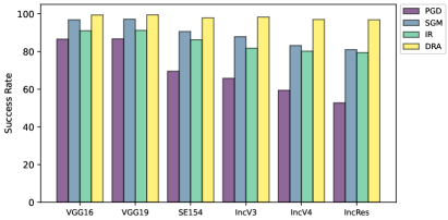
Figure 5: Transferability against different models: the success rates of black-box attacks (untargeted) crafted on an ensemble of 3 models (RN50, RN152 and DN121). The horizontal axis represents different target models.

As shown in Tab. I, the performance of the existing methods is unsatisfactory in some cases. Some works show that the ensemble-based strategy [12] can improve the performance of transfer attacks [13, 50]. Fig. 5 shows the results of the ensemble strategy. We use the ensemble of ResNet-50, ResNet-152 and DenseNet-121 to generate the adversarial attack. The ensemble strategy can enhance the adversarial transferability of different methods, and our DRA still performs the best among the existing methods.

The existing works always evaluate the adversarial transferability with the perturbation restricted by $\ell_{\infty}$ = 16/255. In Fig.6, we compare our DRA with the existing methods with different attack strengths. DRA achieves the best performance with different attack strengths.

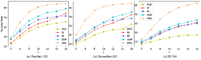
Figure 6: The attack success rate of untargeted transfer attacks on ImageNet. We use the ResNet-50 as the surrogate model and choose three different target models. The horizontal axis represents different attack strengths. Our DRA surpasses the other methods against different target models.

TABLE II: Transferability against secured models. We generate adversarial perturbation (untargeted) by different methods. And then transfer the perturbation to ResNet-50 trained using different secured methods including Augmix [75], Stylized Imagenet[74] and adversarial examples[73]. The best results are in bold.

	Attack	SIN	SIN-IN	Augmix	$\ell_{2}$=0.05	$\ell_{2}$=0.1	$\ell_{\infty}$=0.5	$\ell_{\infty}$=1
RN50	PGD[40]	34.44	84.32	39.64	24.38	12.74	3.64	2.88
	MI [48]	56.98	88.74	64.32	61.78	46.38	27.52	17.88
	TI [49]	38.46	80.28	38.74	26.74	14.12	4.16	3.12
	SGM [13]	49.72	96.18	72.58	58.12	37.02	9.34	5.40
	DRA+PGD	98.08	98.86	98.34	98.70	98.54	88.90	63.16
DN121	PGD[40]	30.74	45.36	32.46	20.5	12.20	4.08	3.06
	MI [48]	40.26	46.22	39.88	27.54	20.48	10.27	4.20
	TI [49]	32.58	45.74	32.22	22.98	14.26	4.54	4.68
	SGM[13]	43.00	58.52	53.40	44.00	34.06	13.14	8.04
	DRA+PGD	97.52	98.54	97.7	98.40	98.14	89.04	66.62
RN152	PGD[40]	29.84	50.76	35.18	22.16	12.48	3.92	3.00
	MI [48]	29.76	50.16	35.10	21.66	12.30	3.96	2.98
	TI [49]	29.74	50.96	35.22	21.8	12.58	3.94	2.98
	SGM[13]	47.62	84.28	69.98	59.92	40.34	11.48	6.12
	DRA+PGD	97.42	98.5	97.62	97.56	77.36	79.82	50.66
DN201	PGD[40]	34.02	50.76	39.08	24.56	14.52	4.46	3.16
	MI [48]	35.11	50.26	38.82	22.46	14.12	4.46	3.14
	TI [49]	34.62	50.83	40.11	22.25	14.28	4.35	3.06
	SGM[13]	49.14	76.32	63.66	52.76	43.12	17.32	10.08
	DRA+PGD	95.42	98.46	97.72	96.54	58.58	65.94	33.10

In Tab. II, we provide experiments to show that the adversarial examples generated by DRA can also effectively penetrate the advanced secured models. Augmix [75] is an augmentation-based training in order to make the model robust to natural corruptions. Training on Stylized ImageNet [74] can increase shape bias and decrease bias towards texture. Adversarial training is considered the most effective way to defend against attacks[73]. As shown in Tab. II, we generate the adversarial perturbation by different methods and then transfer the perturbation to ResNet-50 trained using different secured methods. “$\ell_{2}$=0.05” represents the adversarially trained ResNet-50 using perturbation constrained in $\ell_{2}$ ball with radius $\epsilon=0.05$. The performance of the existing methods will severely degrade when attacking against the robust target model. For transfer ResNet-50 $\rightarrow$ robust model $\ell_{\infty}=1$, the attack success rate of SGM is 5.40$\%$ while our DRA can still achieve a success rate of 63.16$\%$. DRA outperforms the existing methods in attacking the advanced defense models.

TABLE III: Transferability against normal models: the success rates of black-box attacks (targeted) crafted on VGG19, RN50 and DN121. The maximum standard deviation of this experiment is 0.88$\%$ which is much less than our improvement. The best results are in bold.

Model	Attack	VGG19	DN121	RN50	RN152	WRN50-2	SQN	SFN	IncV3
RN50	PGD [40]	1.42$\%$	2.68$\%$	93.77$\%$	2.16$\%$	2.76$\%$	2.05$\%$	1.36$\%$	0.60$\%$
	DI [17]	10.64$\%$	17.54$\%$	99.01$\%$	13.80$\%$	13.75$\%$	1.43$\%$	1.26$\%$	4.12$\%$
	Simple [52]	70.77$\%$	57.78$\%$	100$\%$	59.64$\%$	68.03$\%$	7.92$\%$	6.84$\%$	15.50$\%$
	CDA [20]	73.58$\%$	75.42$\%$	96.45$\%$	72.14$\%$	71.73$\%$	48.62$\%$	42.64$\%$	35.24$\%$
	TTP [21]	81.11$\%$	83.68$\%$	98.13$\%$	83.58$\%$	81.27$\%$	58.02$\%$	54.18$\%$	46.47$\%$
	DRA+PGD	87.80$\%$	94.23$\%$	97.03$\%$	93.85$\%$	91.65$\%$	85.18$\%$	92.14$\%$	75.93$\%$
DN121	PGD [40]	1.28$\%$	97.40$\%$	1.78$\%$	1.01$\%$	1.37$\%$	2.50$\%$	1.58$\%$	0.72$\%$
	DI [17]	7.31$\%$	98.81$\%$	9.06$\%$	5.78$\%$	6.29$\%$	1.28$\%$	1.16$\%$	1.10$\%$
	Simple [52]	50.10$\%$	99.98$\%$	41.74$\%$	24.90$\%$	35.09$\%$	7.57$\%$	4.13$\%$	18.53$\%$
	CDA [20]	45.73$\%$	97.22$\%$	56.85$\%$	46.14$\%$	49.66$\%$	44.62$\%$	32.64$\%$	33.61$\%$
	TTP [21]	60.71$\%$	98.38$\%$	71.00$\%$	59.12$\%$	59.95$\%$	55.42$\%$	36.15$\%$	43.14$\%$
	DRA+PGD	84.83$\%$	97.50$\%$	92.36$\%$	89.84$\%$	88.70$\%$	83.63$\%$	85.68$\%$	75.48$\%$
VGG19	PGD [40]	95.67$\%$	0.31$\%$	0.30$\%$	0.20$\%$	0.25$\%$	0.42$\%$	0.82$\%$	0.45$\%$
	DI [17]	99.38$\%$	3.10$\%$	2.08$\%$	1.02$\%$	1.29$\%$	1.65$\%$	1.14$\%$	0.72$\%$
	Simple [52]	99.90$\%$	13.79$\%$	13.55$\%$	5.16$\%$	7.50$\%$	4.45$\%$	1.39$\%$	7.01$\%$
	CDA [20]	98.30$\%$	17.26$\%$	18.83$\%$	7.73$\%$	10.35$\%$	6.72$\%$	4.25$\%$	5.61$\%$
	TTP [21]	99.13$\%$	46.58$\%$	48.50$\%$	28.55$\%$	33.75$\%$	28.32$\%$	5.97$\%$	14.79$\%$
	DRA+PGD	93.82$\%$	85.65$\%$	84.45$\%$	80.48$\%$	75.25$\%$	87.25$\%$	82.62$\%$	70.58$\%$

IV-C The Evaluation of Targeted Attack

In this section, we focus on targeted attacks. Generating transferable targeted adversarial examples is much more challenging for current compared with untargeted attacks [12, 76]. Liu et al. [12] show that the decision boundaries for the original class of the image of different models align well with each other, which partially explains why untargeted adversarial perturbation can transfer. However, the decision regions for the other classes of different models are very different, which causes the difficulty of obtaining high targeted adversarial transferability by attacking the surrogate model. It is worth noting that different models tend to give the same predictions for images from the same distribution. As shown in Fig. 4, the targeted perturbation generated by DRA contains the features of the target distribution, which may dominate the prediction.

Tab.III shows that our DRA can surpass the previous best targeted transfer attack TTP [21] by a large margin. For transfer ResNet-50 $\rightarrow$ VGG19, DRA achieves a success rate of 87.80$\%$, which is 17.03$\%$ and 6.69$\%$ higher than Simple [52] and TTP, respectively. When transferring from the surrogate model to the target model with quite different architecture, the advantages of DRA are more significant. For transfer ResNet-50 $\rightarrow$ IncV3, DRA achieves a success rate of 75.93$\%$, which is 60.43$\%$ and 29.46$\%$ higher than Simple and TTP, respectively. Meanwhile, we found that Simple [52] performs best when the surrogate and target models have the same architecture. When the architecture of the surrogate and target model is the same, Simple [52] uses the same model to generate perturbation and evaluates the attack performance, which is a white-box attack. Our DRA uses the modified model to generate adversarial perturbation and the target model shares the same architecture with the surrogate model but has different parameters. Thus the attack success rate of DRA is slightly lower than Simple in the white box attack scenario. However, since we focus more on the adversarial transferability between models with different architectures, we argue that this is not a conspicuous drawback of the proposed method.

To evaluate the effectiveness of our DRA comprehensively, we also evaluate its targeted transferability against secured models. Similar to the Sec. IV-B, we consider various types of defense methods (augmented vs. stylized vs. adversarial). As shown in Tab. IV, the secured models can effectively defend the adversarial examples generated by the Simple [52] attack that is a state-of-the-art iterative targeted attack, while our DRA can still penetrate the defense model effectively. For example, for transfer ResNet-50 $\rightarrow$ robust model $\ell_{\infty}=1$, DRA achieves a success rate of 24.22$\%$, which is 23.98$\%$ and 22.98$\%$ higher than Simple and TTP, respectively, validating the superiority of DRA on transfer attacks.

TABLE IV: Transferability against secured models. We generate adversarial perturbation (targeted) by different methods. And then transfer the perturbation to ResNet-50 trained using different secured methods including Augmix [75], Stylized Imagenet[74] and adversarial examples[73]. The best results are in bold.

	Attack	SIN	SIN-IN	Augmix	$\ell_{2}$=0.05	$\ell_{2}$=0.1	$\ell_{\infty}$=0.5	$\ell_{\infty}$=1
VGG19	Simple	0.78	4.60	2.64	0.83	0.22	0.23	0.19
	TTP	47.32	61.52	77.52	68.42	7.14	10.34	0.56
	DRA+PGD	80.00	89.31	79.73	82.93	41.88	48.45	15.34
DN121	Simple	2.27	17.78	10.37	3.70	0.31	0.35	0.24
	TTP	50.48	77.32	78.86	69.08	7.08	12.78	0.65
	DRA+PGD	78.83	92.92	86.74	90.22	52.52	58.43	18.01
RN50	Simple	4.29	67.11	23.08	7.08	0.34	0.53	0.24
	TTP	57.75	92.96	88.79	74.95	7.62	14.23	1.24
	DRA+PGD	88.62	97.41	92.21	94.92	59.42	67.00	24.22

TABLE V: The attack success rates of untargeted black-box attacks on ImageNet crafted on RN50 and DN121. The maximum standard deviation of this experiment is 0.96$\%$ which is much less than our improvement. The best results are in bold.

Source	Attack	Vgg19	RN152	DN121	DN201	SE154	IncV3	IncV4	IncRes
ResNet50	PGD [40]	53.00	61.26	55.62	53.56	24.78	20.86	21.96	17.60
	PGD+DRA	98.26	99.24	99.56	99.28	93.92	95.56	92.66	92.56
	MI [48]	64.86	73.22	73.50	64.33	47.20	39.08	37.35	25.26
	MI+DRA	96.36	97.88	98.68	92.28	92.16	94.06	91.94	91.78
	NI [18]	79.20	84.20	81.56	78.20	55.62	47.96	50.14	39.56
	NI+DRA	96.52	98.34	99.00	98.44	91.76	93.30	90.04	90.14
	SGM [13]	82.87	88.40	83.56	80.34	61.30	53.72	49.83	42.86
	SGM+DRA	97.52	98.58	99.00	98.40	93.04	94.56	91.42	90.42
	SI [18]	75.22	86.46	83.56	79.30	46.46	42.68	41.68	31.50
	SI+DRA	96.80	98.88	99.24	98.82	92.72	95.62	92.94	93.82
	DI [17]	75.06	81.65	81.98	74.80	52.42	42.58	44.30	27.12
	DI+DRA	98.88	98.94	99.34	99.06	96.28	96.80	95.02	94.02
Source	Attack	Vgg19	RN50	RN152	DN201	SE154	IncV3	IncV4	IncRes
DenseNet121	PGD [40]	56.78	58.22	43.76	65.98	23.46	21.92	23.82	17.64
	PGD+DRA	98.32	99.46	98.78	99.22	94.80	95.52	93.60	92.24
	MI [48]	68.36	74.18	67.88	79.56	55.58	49.22	42.35	32.24
	MI+DRA	96.60	98.44	97.28	98.38	92.30	93.62	91.88	89.90
	NI [18]	83.72	86.08	74.98	89.84	62.36	54.66	56.90	43.78
	NI+DRA	96.98	98.88	97.96	98.76	92.62	92.78	90.40	88.18
	SGM [13]	80.18	88.54	80.54	92.70	64.92	54.62	49.82	37.76
	SGM+DRA	92.16	94.76	90.98	93.04	82.60	79.58	76.18	70.22
	SI [18]	76.58	80.90	69.08	88.64	48.68	46.08	45.24	33.52
	SI+DRA	97.64	99.28	98.66	99.34	94.74	95.90	94.06	93.68
	DI [17]	73.68	79.56	71.72	80.40	53.34	49.65	43.94	31.72
	DI+DRA	98.94	99.34	98.42	99.18	95.90	95.76	94.78	92.16

IV-D The Compatibility of DRA with Other Attacks

Various techniques have been proposed to improve the transferability of adversarial attacks, such as advanced gradient calculations [48, 18, 13], and input transformations [17, 18]. In the previous subsections, we mainly show that our DRA method can significantly improve the performance of the widely used baseline attack PGD[40]. Here, we delve into the compatibility of our DRA method with other attack methods. In Tab.V, we compare the adversarial transferability of the original adversarial attacks and the DRA version of these attacks. ”PGD” means the PGD attack generated with the normal pre-trained surrogate models and ”PGD+DRA” means the PGD attack generated by our DRA fine-tuned surrogate models. Our DRA fine-tuning method can significantly improve the performance of different baseline attacks. Moreover, incorporating DRA with the input transformations based attacks (SI, DI) achieves better performance than the advanced gradient based attacks (MI, NI, SGM). We think the advanced gradient based attacks somewhat change the gradient of the model which may increase the DCG in our fine-tuned models.

IV-E Transfer-based Attack on Google Cloud Vision

In this section, we evaluate our DRA attack in the more challenging case, attacking a real-world computer vision system (the Google Cloud Vision API). Most existing works fool real-world computer vision systems with query-based attacks, which require a large number of queries [46, 77, 78]. In contrast, we apply the transfer-based attack to fool the Google Cloud Vision API. Specifically, we use the ResNet-50 as the surrogate model to generate the adversarial examples and then use the Google Cloud Vision API to predict these examples. The API predicts a list of semantic labels along with confidence scores. We measure both the targeted and untargeted transferability. For the untargeted attack, we measure whether or not the ground-truth class appeared in the returned list. For the targeted attack, we measure whether or not the target class appeared in the returned list. Since the predicted label space of Google Cloud Vision API does not precisely correspond to the 1000 ImageNet classes, we treated semantically similar classes as the same, following the setting in [52]. We take the evaluation on randomly selected 500 images that originally yield correct predictions. Fig.7 shows the targeted adversarial examples generated by our method and the top-5 predictions made by the Google Cloud Vision API, the hamster and the arctic fox are misclassified as corn by the Google Cloud Vision API. We compare our method with the original PGD and the previous best iterative transfer attack method Simple [52] in Tab.VI. In particular, DRA achieves the best attack performance compared with previous attack methods. This demonstrates the high practicality of our method which can even attack real-world computer vision systems with a high success rate, e.g., Google Cloud Vision API.

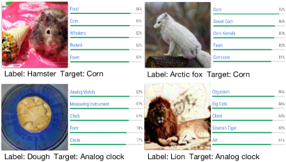
Figure 7: We show that the adversarial perturbation generated by our DRA is imperceptible to human observers but can successfully fool the Google Cloud Vision with the target class.

TABLE VI: Untargeted and targeted transfer attack success rates ($\%$) of different attacks on Google Cloud Vision.

	PGD [40]	Simple[52]	DRA
Untargeted	50.6	51.8	86.6
Targeted	8.2	19.4	48.6

IV-F Evaluation on the Other Datasets

IV-F1 The Evaluation on ImageNet-V2

In this subsection, we evaluate our method on the ImageNet-V2 with 10000 images [61] which are independent of existing pre-trained models. As shown in Tab.VII, our DRA method surpasses the other methods by a large margin. As for transfer from ResNet-50 to Inception-V3, DRA can improve the performance of the baseline method PGD from $59.47\%$ to $99.24\%$.

TABLE VII: The attack success rates of untargeted black-box attacks on ImageNet V2 crafted on RN50 and DN121. The maximum standard deviation of this experiment is 0.84$\%$ which is much less than our improvement. The best results are in bold.

Source	Attack	VGG19	RN152	DN121	DN201	SE154	IncV3	IncV4	IncRes
ResNet50	PGD [40]	83.34	86.20	84.04	80.29	65.51	59.47	59.43	52.45
	DI [17]	95.44	89.95	90.72	87.91	79.29	74.16	74.47	62.47
	MI [48]	92.67	94.34	94.30	93.18	82.87	75.98	74.34	67.25
	SGM [13]	95.34	95.52	93.84	91.55	82.99	75.56	73.14	62.88
	DRA+PGD	99.39	99.66	99.81	99.76	98.11	99.24	98.30	98.14
Source	Attack	VGG19	RN50	RN152	DN201	SE154	IncV3	IncV4	IncRes
DenseNet121	PGD [40]	86.23	87.13	80.21	90.07	68.57	63.02	63.58	54.71
	DI [17]	95.35	91.41	84.41	91.89	80.16	73.85	76.17	63.96
	MI [48]	93.77	93.99	89.71	96.41	83.92	77.22	76.38	68.93
	SGM [13]	94.91	95.89	91.51	96.78	84.75	76.58	75.67	64.97
	DRA+PGD	99.41	99.71	99.62	99.82	98.04	98.76	98.09	97.52

IV-F2 The Evaluation on CIFAR-10

Following the existing works [13, 50, 52], we focus on addressing the transferability on the ImageNet dataset in the previous subsection. In this subsection, we conduct experiments on another dataset (CIFAR-10) to verify the effectiveness of the DRA algorithm further. We use the ResNet-18 as the surrogate model and choose three target models with different architecture (VGG19, DenseNet-121 and ShuffleNetV2). We set the step size $\alpha$ to $2/255$, and set the iteration steps to $N=10$. As shown in Fig. 8, our DRA shows better transferability than existing transfer attacks. For transfer ResNet-18 $\rightarrow$ VGG19 with attack strength $\epsilon=4/255$, DRA can achieve a success rate of 61.97$\%$ which is 13.62$\%$ higher than SGM [13] and 18.48$\%$ higher than PGD [40]. So far, we have evaluated the effectiveness of our DRA on the large-scale datasets (ImageNet) and small-scale datasets (CIFAR-10).

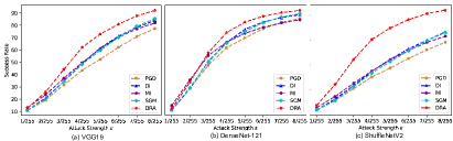
Figure 8: The attack success rate of transfer attacks on CIFAR-10. We illustrate the attack success rate for different methods on CIFAR-10. We use the ResNet-18 as the surrogate model and choose three different target models. The horizontal axis represents different attack strengths. Our DRA surpass the other methods against different target models.

V Discussion

V-A Understanding the superiority of DRA

The superiority of DRA can be understood from two aspects. First, DRA reduces the dependency on the surrogate model. The existing transfer attacks usually regard the over-fitting on the surrogate models as the hindering factor of adversarial transferability and devote to alleviating the over-fitting by improving the optimization algorithm. Our proposed method seeks the commonality among different models from the data distribution perspective for that the ground truth data distribution is model-independent. Our method alleviates this over-fitting by aligning the gradient of the model with the gradient of the ground-truth data distribution. In this way, DRA can effectively reduce the dependence on the surrogate model and generate high transferable adversarial examples. Fig.9 illustrates the frequency histograms of Pearson Correlation Coefficient (PCC) [79] between the adversarial perturbations generated through different models with the same input. The correlation of the adversarial perturbations generated through different models using the PGD [40] attack is around zero, which confirms that the perturbations generated by the original PGD is specific to different surrogate models. The adversarial perturbations generated by different models using our DRA show a stronger correlation than other existing methods, which means that our DRA can effectively reduce the dependency of the perturbation on the surrogate model.

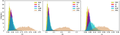
Figure 9: The frequency histogram of the Pearson correlation coefficient (PCC) between adversarial perturbations of the same image generated by the surrogate models ResNet-50 and ResNet-152 (a), ResNet-50 and DenseNet-121 (b), and DenseNet-121 and DenseNet-201 (c). Higher PCC indicates a greater positive correlation. The perturbations generated by our DRA method are closer to each other with different surrogate models than perturbations generated by other methods.

Second, our proposed method intrinsically changes the distribution of input images, leading to more transferable adversarial images. To be specific, our untargeted attack moves the image out of its original distribution, making it difficult for classifiers to classify the image correctly. Fig.2 shows that the untargeted adversarial examples generated by our DRA are regarded as the out-of-distribution examples by the OOD detection method [29]. Out-of-distribution examples can mislead the deep models and cause safety concerns [29, 80]. Our targeted attack can effectively iteratively imprint the features of the target distribution on the image, leading different classifiers to misclassify the image as the target class. For example, Fig.1 shows that the targeted adversarial perturbation generated by our method contains recognizable features of the target distribution that dominates the classification. However, the adversarial example generated by the normal PGD [40] does not contain the semantic features of the target class.

V-B Compared with Other Fine-tuning Methods

Our fine-tuning method aims to match the direction of the adversarial attack to the gradient of the ground truth data distribution, which is different from the other fine-tuning methods that aim to improve the generalization of models. In Tab.VIII, we compare the test accuracy and the adversarial transferability of different ResNet-50 models. “AugMix” means the ResNet-50 fine-tuned with the data processing technique AugMix [75], “AutoAug” means the ResNet-50 fine-tuned with fast AutoAugment [81] and “MEALV2” means the ResNet-50 fine-tuned with the knowledge distillation method MEALV2 [82] that achieves 80$\%$+ Top-1 accuracy on ResNet-50. Our method reduces the test accuracy of the surrogate model but greatly enhances the adversarial transferability. This experiment shows that the generalization (test accuracy) of the model may not the key factor for adversarial transferability.

TABLE VIII: The Top-1 test accuracy and the success rates of untargeted PGD attacks for different ResNet-50 models. The best results are in bold.

Model	Acc	VGG19	RN152	DN121	SE154	IncV3
Original	76.13	53.00	61.26	55.62	24.78	20.86
AugMix	77.53	55.90	56.46	54.18	34.10	27.72
AutoAug	77.60	50.18	45.76	39.14	19.12	16.48
MEALV2	80.67	42.40	35.32	39.16	25.56	19.38
DRA	61.06	98.26	99.24	99.56	93.92	95.56

V-C The influence of the hyperparameter

In this subsection, we show that decreasing the distance between the gradient of the surrogate model and the gradient of the ground truth data distribution enhances adversarial transferability, whereas increasing this distance has the opposite effect. As shown in Eq. 11 and our Alg. 1, our proposed method DRA has one hyperparameter $\lambda$. We optimize the classification loss and the DCG loss jointly during fine-tuning and adjust the strength of DCG loss through the hyperparameter $\lambda$. Fig. 10 shows the influence of $\lambda$. If $\lambda$ is less than 0, the distance between the input-gradients of the surrogate model and the gradients of the ground truth data distribution is increased, and the adversarial transferability drops dramatically. If $\lambda$ is greater than 0, the distance between the input-gradients of the surrogate model and the gradients of the ground truth data distribution is decreased, and the adversarial transferability is improved. Meanwhile, the relationship between the adversarial transferability and $\lambda$ is not monotonic. Too large $\lambda$ may restrict the model’s capability of learning classification-related features.

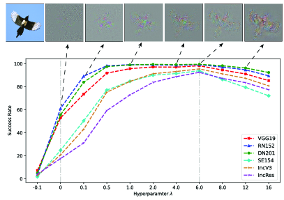
Figure 10: We illustrate the attack success rate (untargeted) when generating adversarial perturbation by different DRA fine-tuned models. “$\lambda$=1.0” represents the model fine-tuned with hyperparameter $\lambda$=1. We also present a seagull’s adversarial perturbation generated by different DRA fine-tuned models.

V-D t-SNE visualizations

To find out whether the generated adversarial examples have attacked the target model in the desired way. We visualize the feature embeddings of both the clean images (red) and their corresponding adversarial examples (green) using t-SNE [83]. To be specific, we use the ResNet-50 (surrogate model) to generate untargeted adversarial examples and use the DenseNet-121 (target model) to obtain the final latent representation. Further distance indicates better performance for the untargeted attack. As shown in Fig. 11, though the final latent representations of the adversarial examples generated by SGM show more difference with the clean images than PGD, our method yields features that clearly separate the clean and adversarial images, compared with PGD [40] and SGM [13]. This further validates the superiority of our proposed DRA.

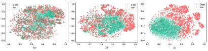
Figure 11: t-SNE visualizations. We illustrate the t-SNE plots for clean (red) images and their adversarial (green) examples. (a) PGD. (b) SGM. (c) DRA (Ours).

VI Conclusion

In this paper, we propose a novel understanding of adversarial transferability from the data distribution perspective. We find that moving the image out of its original distribution can enhance the untargeted adversarial transferability and dragging the image toward the target distribution contributes to high targeted adversarial transferability. We propose a method named Distribution-Relevant Attack (DRA), which apply a fine-tuned surrogate model to generate more transferable adversarial images with data-distribution relevant information. Technically, we propose to fine-tune the surrogate model with a gradient matching method to match the gradient of the model and the gradient of the data distribution, which enables us to push the image away from its original distribution with the gradient of the model. Extensive experiments demonstrate that the proposed DRA establishes state-of-the-art performance in both untargeted and targeted attack scenarios. Moreover, DRA can also effectively fool the real-world computer vision system (the Google Cloud Vision API). Our finding not only motivates researchers to rethink the adversarial transferability from a data distribution perspective but also provides a strong counterpart for future research on adversarial defense.

Proof of the intergration by parts formula

We assume that $g(\boldsymbol{x})$ and $f(\boldsymbol{x})$ are differentiable in Eq. (7). We can get the following equation:

$$\nabla_{{x_{i}}}[g(\boldsymbol{x})\nabla_{{x_{i}}}f(\boldsymbol{x})] =\nabla_{{x_{i}}}g(\boldsymbol{x})\nabla_{{x_{i}}}f(\boldsymbol{x})+g(\boldsymbol{x})\nabla_{{x_{i}}}^{2}f(\boldsymbol{x}).$$ (14)

We consider this as a function of $x_{i}$ alone, all other variables being fixed. Then, integrating over $x_{i}\in\mathbb{R}$, we get the equation:

$$\lim_{M\to\infty}g({\boldsymbol{x}})\nabla_{{x_{i}}}f({\boldsymbol{x}})|_{-\boldsymbol{M}_{i}}^{+\boldsymbol{M}_{i}} =\int_{-\infty}^{+\infty}\nabla_{{x_{i}}}f(\boldsymbol{x})\nabla_{{x_{i}}}g(\boldsymbol{x})d{x_{i}}$$ (15)

$$+\int_{-\infty}^{+\infty}g(\boldsymbol{x})\nabla_{{x_{i}}}^{2}f(\boldsymbol{x})dx_{i},$$

which can prove the Eq. (7). “+$\boldsymbol{M}_{i}$” represents the vector $[x_{1},...,x_{i-1},+M,x_{i+1},...,x_{n}]$. “-$\boldsymbol{M}_{i}$” represents the vector $[x_{1},...,x_{i-1},-M,x_{i+1},...,x_{n}]$.

Detailed Derivation of the Equation (6)

$$\int_{-\infty}^{+\infty}p_{D}(y)dy\int_{\boldsymbol{x}\in\mathbb{R}^{n}}(\nabla_{\boldsymbol{x}}\log p_{\theta}(y|\boldsymbol{x})^{\rm{T}}\cdot\nabla_{\boldsymbol{x}}\log p_{D}({\boldsymbol{x}}|y))p_{D}(\boldsymbol{x}|y)d\boldsymbol{x}$$ (16)

$$\overset{\text{(I)}}{=}\int_{-\infty}^{+\infty}p_{D}(y)dy\int_{\boldsymbol{x}\in\mathbb{R}^{n}}(\nabla_{\boldsymbol{x}}\log p_{\theta}(y|\boldsymbol{x})^{\rm{T}}\cdot\nabla_{\boldsymbol{x}}p_{D}({\boldsymbol{x}}|y))d\boldsymbol{x}$$

$$\overset{\text{(II)}}{=}\int_{-\infty}^{+\infty}p_{D}(y)dy\sum_{i=1}^{n}\int_{\boldsymbol{x}\in\mathbb{R}^{n}}\nabla_{{x_{i}}}\log p_{\theta}(y|\boldsymbol{x})\nabla_{{x_{i}}}p_{D}({\boldsymbol{x}}|y)d{\boldsymbol{x}}$$

$$=\int_{-\infty}^{+\infty}p_{D}(y)dy\sum_{i=1}^{n}\int_{\tilde{\boldsymbol{x}}_{i}\in\mathbb{R}^{n-1}}[\int_{-\infty}^{+\infty}\nabla_{{x_{i}}}\log p_{\theta}(y|\boldsymbol{x})\nabla_{{x_{i}}}p_{D}({\boldsymbol{x}}|y)d{x_{i}}]d{\tilde{\boldsymbol{x}}_{i}}$$

$$\overset{\text{(III)}}{=}\int_{-\infty}^{+\infty}p_{D}(y)dy\sum_{i=1}^{n}\int_{\tilde{\boldsymbol{x}}_{i}\in\mathbb{R}^{n-1}}[\lim_{M\to\infty}p_{D}(\boldsymbol{x}|y)\nabla_{x_{i}}\log p_{\theta}(y|\boldsymbol{x})|_{-\boldsymbol{M}_{i}}^{+\boldsymbol{M}_{i}}]d{\tilde{\boldsymbol{x}}_{i}}$$

$$\quad-\int_{-\infty}^{+\infty}p_{D}(y)dy\sum_{i=1}^{n}\int_{\tilde{\boldsymbol{x}}_{i}\in\mathbb{R}^{n-1}}[\int_{-\infty}^{+\infty}p_{D}(\boldsymbol{x}|y)\nabla^{2}_{x_{i}}\log p_{\theta}(y|\boldsymbol{x})d{x_{i}}]d{\tilde{\boldsymbol{x}}_{i}}$$

$$=\int_{-\infty}^{+\infty}p_{D}(y)dy\sum_{i=1}^{n}\int_{\tilde{\boldsymbol{x}}_{i}\in\mathbb{R}^{n-1}}[\lim_{M\to\infty}p_{D}(\boldsymbol{x}|y)\nabla_{x_{i}}\log p_{\theta}(y|\boldsymbol{x})|_{-\boldsymbol{M}_{i}}^{+\boldsymbol{M}_{i}}]d{\tilde{\boldsymbol{x}}_{i}}$$

$$\quad-\int_{-\infty}^{+\infty}p_{D}(y)dy\sum_{i=1}^{n}\int_{\boldsymbol{x}\in\mathbb{R}^{n}}[p_{D}(\boldsymbol{x}|y)\nabla^{2}_{x_{i}}\log p_{\theta}(y|\boldsymbol{x})]d{\boldsymbol{x}}$$

$$=\int_{-\infty}^{+\infty}p_{D}(y)dy\sum_{i=1}^{n}\int_{\tilde{\boldsymbol{x}}_{i}\in\mathbb{R}^{n-1}}[\lim_{M\to\infty}p_{D}(\boldsymbol{x}|y)\nabla_{x_{i}}\log p_{\theta}(y|\boldsymbol{x})|_{-\boldsymbol{M}_{i}}^{+\boldsymbol{M}_{i}}]d{\tilde{\boldsymbol{x}}_{i}}$$

$$\quad-\mathbb{E}_{p_{D}(y)}\mathbb{E}_{p_{D}({\boldsymbol{x}}|y)}[{\rm{tr}}(\nabla^{2}_{\boldsymbol{x}}\log p_{\theta}(y|{\boldsymbol{x}}))]$$

$$\overset{\text{(IV)}}{=}-\mathbb{E}_{p_{D}(y)}\mathbb{E}_{p_{D}({\boldsymbol{x}}|y)}\left[{\rm{tr}}(\nabla^{2}_{\boldsymbol{x}}\log p_{\theta}(y|{\boldsymbol{x}}))\right],$$

where $\nabla^{2}_{\boldsymbol{x}}$ denotes the Hessian with respect to $\boldsymbol{x}$. “+$\boldsymbol{M}_{i}$” represents the vector $[x_{1},...,x_{i-1},+M,x_{i+1},...,x_{n}]$. “-$\boldsymbol{M}_{i}$” represents the vector $[x_{1},...,x_{i-1},-M,x_{i+1},...,x_{n}]$. $\boldsymbol{x}=[x_{1},...,x_{n}]$ is an n-dimensional vector. $\tilde{\boldsymbol{x}}_{i}=[x_{1},...,x_{i-1},x_{i+1},...,x_{n}]$.

We use the formula: $\nabla_{x}\log f(x)=f(x)^{-1}\nabla_{x}f(x)$ for equality (I). In equality (I), $\nabla_{\boldsymbol{x}}\log p_{\theta}(y|\boldsymbol{x})^{\rm{T}}$ and $\nabla_{\boldsymbol{x}}\log p_{D}({\boldsymbol{x}}|y)$ are n-dimensional vectors, and their product result is a scalar. We use the formula: $\boldsymbol{u}^{T}\cdot\boldsymbol{v}=\sum_{i=1}^{n}u_{i}v_{i}$ for equality (II), where n represents the dimension of the data. As for equality (III), we use the integration by parts formula. The equality (IV) holds for that we assume $p_{D}({\boldsymbol{x}}|y)\rightarrow 0$ when $||\boldsymbol{x}||_{2}\rightarrow\infty$.

References

- Raghavendra et al. [2015] R. Raghavendra, K. B. Raja, and C. Busch, “Presentation attack detection for face recognition using light field camera,” IEEE Trans. Image Process., vol. 24, no. 3, pp. 1060–1075, 2015. [Online]. Available: https://doi.org/10.1109/TIP.2015.2395951
- Guo et al. [2021] J. Guo, X. Zhu, Z. Lei, and S. Z. Li, “Decomposed meta batch normalization for fast domain adaptation in face recognition,” IEEE Trans. Inf. Forensics Secur., vol. 16, pp. 3082–3095, 2021. [Online]. Available: https://doi.org/10.1109/TIFS.2021.3073823
- Arashloo [2021] S. R. Arashloo, “Matrix-regularized one-class multiple kernel learning for unseen face presentation attack detection,” IEEE Trans. Inf. Forensics Secur., vol. 16, pp. 4635–4647, 2021. [Online]. Available: https://doi.org/10.1109/TIFS.2021.3111766
- Sun et al. [2021] Z. Sun, S. Balakrishnan, L. Su, A. Bhuyan, P. Wang, and C. Qiao, “Who is in control? practical physical layer attack and defense for mmwave-based sensing in autonomous vehicles,” IEEE Trans. Inf. Forensics Secur., vol. 16, pp. 3199–3214, 2021. [Online]. Available: https://doi.org/10.1109/TIFS.2021.3076287
- Chen et al. [2019] Y. Chen, C. Dong, P. Palanisamy, P. Mudalige, K. Muelling, and J. M. Dolan, “Attention-based hierarchical deep reinforcement learning for lane change behaviors in autonomous driving,” in IEEE Conference on Computer Vision and Pattern Recognition Workshops. Computer Vision Foundation / IEEE, 2019, pp. 1326–1334. [Online]. Available: http://openaccess.thecvf.com/content_CVPRW_2019/html/WAD/Chen_Attention-Based_Hierarchical_Deep_Reinforcement_Learning_for_Lane_Change_Behaviors_in_CVPRW_2019_paper.html
- Milz et al. [2018] S. Milz, G. Arbeiter, C. Witt, B. Abdallah, and S. K. Yogamani, “Visual SLAM for automated driving: Exploring the applications of deep learning,” in 2018 IEEE Conference on Computer Vision and Pattern Recognition Workshops. Computer Vision Foundation IEEE Computer Society, 2018, pp. 247–257. [Online]. Available: http://openaccess.thecvf.com/content_cvpr_2018_workshops/w9/html/Milz_Visual_SLAM_for_CVPR_2018_paper.html
- Alanís et al. [2021] A. G. Alanís, J. A. G. López, S. P. Dubagunta, A. M. Peinado, and M. Magimai-Doss, “On joint optimization of automatic speaker verification and anti-spoofing in the embedding space,” IEEE Trans. Inf. Forensics Secur., vol. 16, pp. 1579–1593, 2021. [Online]. Available: https://doi.org/10.1109/TIFS.2020.3039045
- Aljasem et al. [2021] M. Aljasem, A. Irtaza, H. Malik, N. Saba, A. Javed, K. M. Malik, and M. Meharmohammadi, “Secure automatic speaker verification (SASV) system through sm-altp features and asymmetric bagging,” IEEE Trans. Inf. Forensics Secur., vol. 16, pp. 3524–3537, 2021. [Online]. Available: https://doi.org/10.1109/TIFS.2021.3082303
- Joshi et al. [2021a] S. Joshi, J. Villalba, P. Zelasko, L. Moro-Velázquez, and N. Dehak, “Study of pre-processing defenses against adversarial attacks on state-of-the-art speaker recognition systems,” IEEE Trans. Inf. Forensics Secur., vol. 16, pp. 4811–4826, 2021. [Online]. Available: https://doi.org/10.1109/TIFS.2021.3116438
- Szegedy et al. [2013] C. Szegedy, W. Zaremba, I. Sutskever, J. Bruna, D. Erhan, I. Goodfellow, and R. Fergus, “Intriguing properties of neural networks,” International Conference on Learning Representations, 2013.
- Goodfellow et al. [2015] I. J. Goodfellow, J. Shlens, and C. Szegedy, “Explaining and harnessing adversarial examples,” International Conference on Learning Representations, 2015.
- Liu et al. [2017] Y. Liu, X. Chen, C. Liu, and D. Song, “Delving into transferable adversarial examples and black-box attacks,” International Conference on Learning Representations, 2017.
- Wu et al. [2019] D. Wu, Y. Wang, S.-T. Xia, J. Bailey, and X. Ma, “Skip connections matter: On the transferability of adversarial examples generated with resnets,” in International Conference on Learning Representations, 2019.
- Su et al. [2018] D. Su, H. Zhang, H. Chen, J. Yi, P.-Y. Chen, and Y. Gao, “Is robustness the cost of accuracy?–a comprehensive study on the robustness of 18 deep image classification models,” in Proceedings of the European Conference on Computer Vision (ECCV), 2018, pp. 631–648.
- Wu and Zhu [2020] L. Wu and Z. Zhu, “Towards understanding and improving the transferability of adversarial examples in deep neural networks,” in Asian Conference on Machine Learning. PMLR, 2020, pp. 837–850.
- Yang et al. [2021a] Z. Yang, L. Li, X. Xu, S. Zuo, Q. Chen, B. Rubinstein, C. Zhang, and B. Li, “Trs: Transferability reduced ensemble via encouraging gradient diversity and model smoothness,” Advances in Neural Information Processing Systems, vol. 34, 2021.
- Xie et al. [2019] C. Xie, Z. Zhang, Y. Zhou, S. Bai, J. Wang, Z. Ren, and A. L. Yuille, “Improving transferability of adversarial examples with input diversity,” in Proceedings of the IEEE/CVF Conference on Computer Vision and Pattern Recognition, 2019, pp. 2730–2739.
- Lin et al. [2019] J. Lin, C. Song, K. He, L. Wang, and J. E. Hopcroft, “Nesterov accelerated gradient and scale invariance for adversarial attacks,” in International Conference on Learning Representations, 2019.
- Wang et al. [2021a] X. Wang, X. He, J. Wang, and K. He, “Admix: Enhancing the transferability of adversarial attacks,” CoRR, vol. abs/2102.00436, 2021. [Online]. Available: https://arxiv.org/abs/2102.00436
- Naseer et al. [2019] M. M. Naseer, S. H. Khan, M. H. Khan, F. Shahbaz Khan, and F. Porikli, “Cross-domain transferability of adversarial perturbations,” Advances in Neural Information Processing Systems, vol. 32, pp. 12 905–12 915, 2019.
- Naseer et al. [2021] M. Naseer, S. Khan, M. Hayat, F. S. Khan, and F. Porikli, “On generating transferable targeted perturbations,” in Proceedings of the IEEE/CVF International Conference on Computer Vision, 2021.
- Huang et al. [2019] Q. Huang, I. Katsman, H. He, Z. Gu, S. Belongie, and S.-N. Lim, “Enhancing adversarial example transferability with an intermediate level attack,” in Proceedings of the IEEE/CVF International Conference on Computer Vision, 2019, pp. 4733–4742.
- Wald et al. [2021] Y. Wald, A. Feder, D. Greenfeld, and U. Shalit, “On calibration and out-of-domain generalization,” Advances in neural information processing systems, vol. 34, pp. 2215–2227, 2021.
- Nagarajan et al. [2020] V. Nagarajan, A. Andreassen, and B. Neyshabur, “Understanding the failure modes of out-of-distribution generalization,” in International Conference on Learning Representations, 2020.
- Hyvärinen [2005] A. Hyvärinen, “Estimation of non-normalized statistical models by score matching,” Journal of Machine Learning Research, vol. 6, no. 24, pp. 695–709, 2005. [Online]. Available: http://jmlr.org/papers/v6/hyvarinen05a.html
- Song et al. [2020] Y. Song, S. Garg, J. Shi, and S. Ermon, “Sliced score matching: A scalable approach to density and score estimation,” in Uncertainty in Artificial Intelligence. PMLR, 2020, pp. 574–584.
- Song and Ermon [2019] Y. Song and S. Ermon, “Generative modeling by estimating gradients of the data distribution,” Advances in Neural Information Processing Systems, vol. 32, 2019.
- Zhu et al. [2021] Y. Zhu, J. Ma, J. Sun, Z. Chen, R. Jiang, Y. Chen, and Z. Li, “Towards understanding the generative capability of adversarially robust classifiers,” in Proceedings of the IEEE/CVF International Conference on Computer Vision, 2021, pp. 7728–7737.
- Liu et al. [2020] W. Liu, X. Wang, J. Owens, and Y. Li, “Energy-based out-of-distribution detection,” Advances in Neural Information Processing Systems, 2020.
- Zhong and Deng [2021] Y. Zhong and W. Deng, “Towards transferable adversarial attack against deep face recognition,” IEEE Trans. Inf. Forensics Secur., vol. 16, pp. 1452–1466, 2021. [Online]. Available: https://doi.org/10.1109/TIFS.2020.3036801
- Komkov and Petiushko [2021] S. Komkov and A. Petiushko, “Advhat: Real-world adversarial attack on arcface face id system,” in 2020 25th International Conference on Pattern Recognition (ICPR). IEEE, 2021, pp. 819–826.
- Wang et al. [2021b] G. Wang, H. Han, S. Shan, and X. Chen, “Unsupervised adversarial domain adaptation for cross-domain face presentation attack detection,” IEEE Trans. Inf. Forensics Secur., vol. 16, pp. 56–69, 2021. [Online]. Available: https://doi.org/10.1109/TIFS.2020.3002390
- Ma et al. [2021] X. Ma, Y. Niu, L. Gu, Y. Wang, Y. Zhao, J. Bailey, and F. Lu, “Understanding adversarial attacks on deep learning based medical image analysis systems,” Pattern Recognition, vol. 110, p. 107332, 2021.
- Finlayson et al. [2019] S. G. Finlayson, J. D. Bowers, J. Ito, J. L. Zittrain, A. L. Beam, and I. S. Kohane, “Adversarial attacks on medical machine learning,” Science, vol. 363, no. 6433, pp. 1287–1289, 2019. [Online]. Available: https://www.science.org/doi/abs/10.1126/science.aaw4399
- Joshi et al. [2021b] S. Joshi, J. Villalba, P. Zelasko, L. Moro-Velázquez, and N. Dehak, “Study of pre-processing defenses against adversarial attacks on state-of-the-art speaker recognition systems,” IEEE Trans. Inf. Forensics Secur., vol. 16, pp. 4811–4826, 2021. [Online]. Available: https://doi.org/10.1109/TIFS.2021.3116438
- Kreuk et al. [2018] F. Kreuk, Y. Adi, M. Cisse, and J. Keshet, “Fooling end-to-end speaker verification with adversarial examples,” in 2018 IEEE International Conference on Acoustics, Speech and Signal Processing (ICASSP), 2018, pp. 1962–1966.
- Morgulis et al. [2019] N. Morgulis, A. Kreines, S. Mendelowitz, and Y. Weisglass, “Fooling a real car with adversarial traffic signs,” arXiv preprint arXiv:1907.00374, 2019.
- Boloor et al. [2019] A. Boloor, X. He, C. Gill, Y. Vorobeychik, and X. Zhang, “Simple physical adversarial examples against end-to-end autonomous driving models,” in 2019 IEEE International Conference on Embedded Software and Systems (ICESS), 2019, pp. 1–7.
- Kurakin et al. [2016] A. Kurakin, I. Goodfellow, and S. Bengio, “Adversarial examples in the physical world,” arXiv e-prints, pp. arXiv–1607, 2016.
- Madry et al. [2018] A. Madry, A. Makelov, L. Schmidt, D. Tsipras, and A. Vladu, “Towards deep learning models resistant to adversarial attacks,” in International Conference on Learning Representations, 2018.
- Moosavi-Dezfooli et al. [2016] S.-M. Moosavi-Dezfooli, A. Fawzi, and P. Frossard, “Deepfool: a simple and accurate method to fool deep neural networks,” in Proceedings of the IEEE/CVF Conference on Computer Vision and Pattern Recognition, 2016, pp. 2574–2582.
- Wiyatno and Xu [2018] R. Wiyatno and A. Xu, “Maximal jacobian-based saliency map attack,” CoRR, vol. abs/1808.07945, 2018. [Online]. Available: http://arxiv.org/abs/1808.07945
- Carlini and Wagner [2017] N. Carlini and D. Wagner, “Towards evaluating the robustness of neural networks,” in 2017 ieee symposium on security and privacy (sp). IEEE, 2017, pp. 39–57.
- Papernot et al. [2017] N. Papernot, P. McDaniel, I. Goodfellow, S. Jha, Z. B. Celik, and A. Swami, “Practical black-box attacks against machine learning,” in Proceedings of the 2017 ACM on Asia conference on computer and communications security, 2017, pp. 506–519.
- Su et al. [2019] J. Su, D. V. Vargas, and K. Sakurai, “One pixel attack for fooling deep neural networks,” IEEE Transactions on Evolutionary Computation, vol. 23, no. 5, p. 828–841, Oct 2019. [Online]. Available: http://dx.doi.org/10.1109/TEVC.2019.2890858
- Dong et al. [2019a] Y. Dong, H. Su, B. Wu, Z. Li, W. Liu, T. Zhang, and J. Zhu, “Efficient decision-based black-box adversarial attacks on face recognition,” in Proceedings of the IEEE/CVF Conference on Computer Vision and Pattern Recognition, 2019, pp. 7714–7722.
- Yang et al. [2020] J. Yang, Y. Jiang, X. Huang, B. Ni, and C. Zhao, “Learning black-box attackers with transferable priors and query feedback,” Advances in Neural Information Processing Systems, vol. 33, 2020.
- Dong et al. [2018] Y. Dong, F. Liao, T. Pang, H. Su, J. Zhu, X. Hu, and J. Li, “Boosting adversarial attacks with momentum,” in Proceedings of the IEEE/CVF Conference on Computer Vision and Pattern Recognition, 2018, pp. 9185–9193.
- Dong et al. [2019b] Y. Dong, T. Pang, H. Su, and J. Zhu, “Evading defenses to transferable adversarial examples by translation-invariant attacks,” in Proceedings of the IEEE/CVF Conference on Computer Vision and Pattern Recognition, 2019, pp. 4312–4321.
- Wang et al. [2020] X. Wang, J. Ren, S. Lin, X. Zhu, Y. Wang, and Q. Zhang, “A unified approach to interpreting and boosting adversarial transferability,” in International Conference on Learning Representations, 2020.
- Guo et al. [2020] Y. Guo, Q. Li, and H. Chen, “Backpropagating linearly improves transferability of adversarial examples.” in Advances in Neural Information Processing Systems, 2020.
- Zhao et al. [2021] Z. Zhao, Z. Liu, and M. Larson, “On success and simplicity: A second look at transferable targeted attacks,” Advances in Neural Information Processing Systems, vol. 34, pp. 6115–6128, 2021.
- Kanth Nakka and Salzmann [2021] K. Kanth Nakka and M. Salzmann, “Learning transferable adversarial perturbations,” in Thirty-Fifth Conference on Neural Information Processing Systems, 2021.
- Poursaeed et al. [2018] O. Poursaeed, I. Katsman, B. Gao, and S. Belongie, “Generative adversarial perturbations,” in Proceedings of the IEEE/CVF Conference on Computer Vision and Pattern Recognition, 2018, pp. 4422–4431.
- Mopuri et al. [2018] K. R. Mopuri, U. Ojha, U. Garg, and R. V. Babu, “Nag: Network for adversary generation,” in Proceedings of the IEEE/CVF Conference on Computer Vision and Pattern Recognition, 2018.
- LeCun et al. [2006] Y. LeCun, S. Chopra, R. Hadsell, M. Ranzato, and F. J. Huang, “A tutorial on energy-based learning,” To appear in “Predicting Structured Data, vol. 1, p. 0, 2006.
- Welling and Teh [2011] M. Welling and Y. W. Teh, “Bayesian learning via stochastic gradient langevin dynamics,” p. 681–688, 2011.
- Hyvärinen and Dayan [2005] A. Hyvärinen and P. Dayan, “Estimation of non-normalized statistical models by score matching.” Journal of Machine Learning Research, vol. 6, no. 4, 2005.
- Hutchinson [1989] M. F. Hutchinson, “A stochastic estimator of the trace of the influence matrix for laplacian smoothing splines,” Communications in Statistics-Simulation and Computation, vol. 18, no. 3, pp. 1059–1076, 1989.
- Russakovsky et al. [2015] O. Russakovsky, J. Deng, H. Su, J. Krause, S. Satheesh, S. Ma, Z. Huang, A. Karpathy, A. Khosla, M. Bernstein, A. C. Berg, and L. Fei-Fei, “ImageNet Large Scale Visual Recognition Challenge,” International Journal of Computer Vision (IJCV), vol. 115, no. 3, pp. 211–252, 2015.
- Recht et al. [2019] B. Recht, R. Roelofs, L. Schmidt, and V. Shankar, “Do imagenet classifiers generalize to imagenet?” in ICML, 2019.
- Simonyan and Zisserman [2015] K. Simonyan and A. Zisserman, “Very deep convolutional networks for large-scale image recognition,” arXiv preprint 1409.1556, 2015.
- He et al. [2016] K. He, X. Zhang, S. Ren, and J. Sun, “Deep residual learning for image recognition,” in Proceedings of the IEEE/CVF Conference on Computer Vision and Pattern Recognition, 2016, pp. 770–778.
- Huang et al. [2017] G. Huang, Z. Liu, L. Van Der Maaten, and K. Q. Weinberger, “Densely connected convolutional networks,” in Proceedings of the IEEE/CVF Conference on Computer Vision and Pattern Recognition, 2017, pp. 4700–4708.
- Hu et al. [2018] J. Hu, L. Shen, and G. Sun, “Squeeze-and-excitation networks,” in Proceedings of the IEEE/CVF Conference on Computer Vision and Pattern Recognition, 2018, pp. 7132–7141.
- Zagoruyko and Komodakis [2016] S. Zagoruyko and N. Komodakis, “Wide residual networks,” in British Machine Vision Conference 2016. British Machine Vision Association, 2016.
- Iandola et al. [2016] F. N. Iandola, S. Han, M. W. Moskewicz, K. Ashraf, W. J. Dally, and K. Keutzer, “Squeezenet: Alexnet-level accuracy with 50x fewer parameters and¡ 0.5 mb model size,” arXiv preprint arXiv:1602.07360, 2016.
- Ma et al. [2018] N. Ma, X. Zhang, H.-T. Zheng, and J. Sun, “Shufflenet v2: Practical guidelines for efficient cnn architecture design,” in Proceedings of the European conference on computer vision (ECCV), 2018, pp. 116–131.
- Szegedy et al. [2016] C. Szegedy, V. Vanhoucke, S. Ioffe, J. Shlens, and Z. Wojna, “Rethinking the inception architecture for computer vision,” in Proceedings of the IEEE/CVF Conference on Computer Vision and Pattern Recognition, 2016, pp. 2818–2826.
- Szegedy et al. [2017] C. Szegedy, S. Ioffe, V. Vanhoucke, and A. A. Alemi, “Inception-v4, inception-resnet and the impact of residual connections on learning,” in Thirty-first AAAI conference on artificial intelligence, 2017.
- Paszke et al. [2019] A. Paszke, S. Gross, F. Massa, A. Lerer, J. Bradbury, G. Chanan, T. Killeen, Z. Lin, N. Gimelshein, L. Antiga, A. Desmaison, A. Kopf, E. Yang, Z. DeVito, M. Raison, A. Tejani, S. Chilamkurthy, B. Steiner, L. Fang, J. Bai, and S. Chintala, “Pytorch: An imperative style, high-performance deep learning library,” Advances in Neural Information Processing Systems 32, pp. 8024–8035, 2019.
- Dosovitskiy et al. [2021] A. Dosovitskiy, L. Beyer, A. Kolesnikov, D. Weissenborn, X. Zhai, T. Unterthiner, M. Dehghani, M. Minderer, G. Heigold, S. Gelly et al., “An image is worth 16x16 words: Transformers for image recognition at scale,” International Conference on Learning Representations, 2021.
- Salman et al. [2020] H. Salman, A. Ilyas, L. Engstrom, A. Kapoor, and A. Madry, “Do adversarially robust imagenet models transfer better?” in Advances in Neural Information Processing Systems, 2020.
- Geirhos et al. [2019] R. Geirhos, P. Rubisch, C. Michaelis, M. Bethge, F. A. Wichmann, and W. Brendel, “Imagenet-trained CNNs are biased towards texture; increasing shape bias improves accuracy and robustness.” in International Conference on Learning Representations, 2019. [Online]. Available: https://openreview.net/forum?id=Bygh9j09KX
- Hendrycks et al. [2020] D. Hendrycks, N. Mu*, E. D. Cubuk, B. Zoph, J. Gilmer, and B. Lakshminarayanan, “Augmix: A simple method to improve robustness and uncertainty under data shift,” in International Conference on Learning Representations, 2020. [Online]. Available: https://openreview.net/forum?id=S1gmrxHFvB
- Yang et al. [2021b] X. Yang, Y. Dong, T. Pang, H. Su, and J. Zhu, “Boosting transferability of targeted adversarial examples via hierarchical generative networks,” CoRR, vol. abs/2107.01809, 2021.
- Brendel et al. [2018] W. Brendel, J. Rauber, and M. Bethge, “Decision-based adversarial attacks: Reliable attacks against black-box machine learning models,” in International Conference on Learning Representations, 2018.
- Ilyas et al. [2018] A. Ilyas, L. Engstrom, A. Athalye, J. Lin, A. Athalye, L. Engstrom, A. Ilyas, and K. Kwok, “Black-box adversarial attacks with limited queries and information,” in Proceedings of the 35th International Conference on Machine Learning,ICML 2018, 2018.
- Benesty et al. [2009] J. Benesty, J. Chen, Y. Huang, and I. Cohen, “Pearson correlation coefficient,” in Noise reduction in speech processing. Springer, 2009, pp. 1–4.
- Huang et al. [2021] R. Huang, A. Geng, and Y. Li, “On the importance of gradients for detecting distributional shifts in the wild,” in Advances in Neural Information Processing Systems, 2021.
- Lim et al. [2019] S. Lim, I. Kim, T. Kim, C. Kim, and S. Kim, “Fast autoaugment,” in Advances in Neural Information Processing Systems (NeurIPS), 2019.
- Shen and Savvides [2020] Z. Shen and M. Savvides, “Meal v2: Boosting vanilla resnet-50 to 80+ top-1 accuracy on imagenet without tricks,” arXiv preprint arXiv:2009.08453, 2020.
- van der Maaten and Hinton [2008] L. van der Maaten and G. Hinton, “Visualizing data using t-sne,” Journal of Machine Learning Research, vol. 9, pp. 2579–2605, 2008.