Adaptive Control of Unknown Pure Feedback Systems with Pure State Constraints

Abstract

This paper deals with the tracking control problem for a class of unknown pure feedback system with pure state constraints on the state variables and unknown time-varying bounded disturbances. An adaptive controller is presented for such systems for the very first time. The controller is designed using the backstepping method. While designing it, Barrier Lyapunov Functions is used so that the state variables do not contravene its constraints. In order to cope with the unknown dynamics of the system, an online approximator is designed using a neural network with a novel adaptive law for its weight update. In the stability analysis of the system, the time derivative of Lyapunov function involves known virtual control coefficient with unknown direction and to deal with such problem Nussbaum gain is used to design the control law. Furthermore, to make the controller robust and computationally inexpensive, a novel disturbance observer is designed to estimate the disturbance along with neural network approximation error and the time derivative of virtual control input. The effectiveness of the proposed approach is demonstrated through a simulation study on the third-order nonlinear system.

I Introduction

In recent years, the stability of the constrained nonlinear system has attracted much attention in the nonlinear control theory community. The reason behind this is its application in the industrial systems. In real-time systems, constraints can appear in different forms such as performance specification, safety, physical stoppage and saturation, and it is ineludible while designing the controller. Dynamically it can appear as a symmetric or asymmetric bound on states, output and control input of the system.

The traditional controller design for nonlinear unconstrained system lack practicability. In [1], Tee et al. have proposed a controller for nonlinear systems with constant output constraints. To prevent constraints, authors have proposed Barrier Lyapunov Function (BLF), which approach infinity when its argument approach certain limit. In [2], Tee et al. have proposed a BLF based controller for nonlinear systems with time-varying output constraints. With the above pioneering works, researchers have started paying attention in the field of controller design for nonlinear system with constraints. A lot of significant related works have been received in recent years. In [3], Ren et al. have studied a BLF based adaptive controller for a nonlinear system with time-varying constraints on the output. In [4, 5, 6], BLF based controller has been studied to tackle practical output constraint for electrostatic micro-actuators, flexible crane system and a wind turbine system.

With the progress in control of a nonlinear constrained system, in [7] Tee et al. have studied controller design for a nonlinear system with partial state constraint. Liu et al. in [8] and [9] have studied a BLF based adaptive backstepping control for strict feedback and pure-feedback single input single output (SISO) nonlinear system having a static constraint on all the states, respectively. In [10], the authors have studied control of SISO nonlinear system having unknown control gain and static constraint on all the states. In [11, 12], the authors have studied BLF based adaptive control of multi input multi output (MIMO) nonlinear system having static and symmetric constraints on all the states. In [13], the authors have used novel BLF for control of time-varying state constrained SISO nonlinear system. In [14, 15], the authors have studied BLF for MIMO nonlinear systems having time-varying state constraints.

Other than BLF based methodology, numerous efforts have been made, such as error transformation and model predictive control (MPC), by academia and industries to design a controller for the constrained system. In error transformation [16, 17, 18, 19, 20], there is likelihood that use of tangent hyperbolic in prescribed function ends with singularity problem and also under specific conditions of prescribed function, inordinate control input can transgress the prescribed control performance, which may lead to instability. In MPC, constraint is accommodated in control design for linear and nonlinear system within an optimization framework by solving a finite horizon open-loop optimal control problem [21]. Most of the optimal control and MPC need knowledge of the dynamics of plant and are numerical and thus depend mostly on computationally intensive algorithms for solving a control problem [22].

As compared to error transformation and MPC, BLF has been extensively investigated for the controller design of constrained system because of its ease in handling unknown system dynamics, uncertainties and disturbances by integrating robust adaptive backstepping or sliding mode control methodology. So far, the literature related to BLF based controller design has been limited for the system having a static and time-varying constraint on all the states [14, 23, 24, 25]. However, there are still a lot of challenging problems which are yet to be explored by the researchers working in this field for the constrained system. One such problem is to control a system with pure state constraints on the state variable. Pure state constraints are state variable inequality constraints (SVICs), which are expressed in terms of time and the state variables. Such constraints frequently arise in the area of management science and economics, mechanics, and aerospace engineering [26].

The aforementioned problem acts as motivation for this paper. As a solution, we design a BLF based robust adaptive backstepping control law using a neural network (NN) for an unknown nonlinear pure feedback system with pure state constraints and time-varying bounded disturbances. The following are essential steps which outline the design of the controller in this paper:

Similar to traditional backstepping approach, the first step involves the transformation of state variables to error variables using the virtual control input. Second, the construction of error variable inequality constraints (EVICs) for error variables using the SVICs. Third, construction of BLF using EVICs and the calculation of its time derivative. The time derivative of BLF is calculated in an early stage to avoid the unnecessary steps of calculating similar time derivative of BLF in the controller design and stability analysis. The time derivative of BLF involves a virtual control coefficient with unknown direction. To deal with such problem, Nussbaum gains [27, 28, 29] is used in the proposed methodology. The fourth step includes the design of NN for the approximation of unknown function involving uncertain dynamics of the system. The fifth step consists of the design of a disturbance observer for the estimation of disturbances along with the derivative of virtual control input and NN approximation error. Finally, using the stability analysis Nussbaum gain based backstepping control law, and an adaptive law for the weight updates of NN is developed. In brief, our contributions are as follows:

1. As mentioned in Table I, compared to state-of-the-art problems, where the controller is designed for the system with static and time-varying state constraint, here a novel controller is proposed for the system with pure state constraints. Moreover, the system is considered as a pure feedback SISO nonlinear system.

2. A BLF based disturbance observer is proposed to estimate the expression involving derivative of virtual control input, external disturbance and NN approximation error. This makes the controller robust and computationally efficient.

TABLE I: Comparison with state-of-the-art problems

	Types of State Constraint			Structure of Nonlinear Systems
	Constant	Time-varying $\Psi_{i}(t)$	Pure State Constraint $\Psi_{i}(\overline{\xi}_{i},t)$	Strict- feedback	Pure- feedback
[30, 31, 32, 33, 34, 35]	✓	$\times$	$\times$	✓	$\times$
[9, 36, 37]	✓	$\times$	$\times$	$\times$	✓
[38, 39, 40, 41, 42, 43, 44, 15, 14]	$\times$	✓	$\times$	✓	$\times$
[23, 24, 25]	$\times$	✓	$\times$	$\times$	✓
Proposed problem	$\times$	$\times$	✓	$\times$	✓

The paper is organized as follows. In Section II, we present the system description and control objectives. This section also presents some assumptions, definition and Lemmas for the stability analysis of the system. Section III consists of five subsections whose first subsection discusses the construction of EVICs for error variables. The second subsection discusses the construction of BLF and calculation of its time derivative. The third subsection discusses the construction of NN for the approximation of unknown term involved in the time derivative of BLF derived in the second subsection; The fourth subsection discusses the construction of disturbance observer for the robustness of the system, and the fifth subsection discusses the steps to design an adaptive controller using the decoupled backstepping technique. Section IV discusses the theorem for the boundedness of all the signals in the closed-loop of the system. Section V discusses the effectiveness of the proposed methodology using the simulation examples. Finally, Section VI concludes the paper.
Following are some basic notations which will be used throughout the paper:

• $\mathbb{N}_{m}\mathrel{\mathop{\mathchar 58\relax}}=\{1,\ldots,m\}$.

• $arctan(x)=\tan^{-1}x$.

II System description and problem statement

Consider the following SISO nonlinear pure-feedback system

$$\begin{split}\dot{x}_{i}&=f_{i}\left(\bar{x}_{i},x_{i+1}\right)+\beta_{i}x_{i+1}+d_{i}\left(\bar{x}_{i},t\right)\\ \dot{x}_{n}&=f_{n}\left(\bar{x}_{n},u\right)+\beta_{n}u+d_{n}\left(\bar{x}_{n},t\right)\\ y&=x_{1}\end{split}$$ (1)

where $x_{i}\in\mathbb{R}$, $\forall i\in\mathbb{N}_{n},y\in\mathbb{R}$ and $u\in\mathbb{R}$ are the $ith$ state, the output, and the control input of the system, respectively; $\overline{x}_{i}=[x_{1},\ldots,x_{i}]^{T}\in\mathbb{R}^{i}$; $f_{i}\left(\bar{x}_{i},x_{i+1}\right)\in\mathbb{R},\forall i\in\mathbb{N}_{n}$ are smooth unknown nonlinear function; $\beta_{i}\in\mathbb{R}$ and $d_{i}\in\mathbb{R},\forall i\in\mathbb{N}_{n}$ are constant control coefficient and unknown time-varying bounded disturbance, respectively. For simplicity of presentation, denote $x_{n+1}=u$. In this study states are considered to be constrained such that, $\mathinner{\!\left\lvert x_{i}\right\rvert}<\Psi_{i}(\overline{x}_{i},t)$, where $\Psi_{i}\in\mathbb{R}$ is a known nonlinear SVIC on the state variable.
Problem Statement: The control objective of the paper is to design a NN based adaptive controller for (1) such that (i) output $y$ tracks the desired output $y_{d}$; (ii) all the closed-loop signals are guaranteed to be bounded; and (iii) all the system states do not contravene there SVICs.
Following are the assumptions which will be needed to achieve the control objective.
Assumption 1 [10]: The control coefficient $\beta_{i}\neq 0$, $\forall i\in\mathbb{N}_{n}$.
Assumption 2 [27]: The unknown time-varying disturbance $d_{i}(\overline{x}_{i},t)$ is bounded and there exist some positive constant $d_{0}$ such that $\mathinner{\!\left\lvert\dot{d}_{i}(\overline{x}_{i},t)\right\rvert}\leq d_{0}$ $\forall i\in\mathbb{N}_{n}$.
Assumption 3 [45]: If $x_{i}\in L_{\infty}$ then the time derivative of $\frac{\partial\psi}{\partial x_{1}},\ldots,\frac{\partial\psi}{\partial x_{i}}$ exist and it is bounded. Definition 1 [46] : The function $\mathcal{N}(\zeta)$ is said to be Nussbaum, if it holds the following property:

$$\begin{split}\underset{s\rightarrow\infty}{\lim}\sup\frac{1}{s}\int_{0}^{s}\mathcal{N}(\zeta)d\zeta=+\infty\\ \underset{s\rightarrow\infty}{\lim}\inf\frac{1}{s}\int_{0}^{s}\mathcal{N}(\zeta)d\zeta=-\infty.\end{split}$$ (2)

There are many functions which can be considered as a Nussbaum function such as $e^{\zeta^{2}}\cos((\pi/2)\zeta)$ and $\zeta^{2}cos(\zeta)$. In this paper, we have used $\mathcal{N}(\zeta)=\zeta^{2}cos(\zeta)$ as a Nussbaum function.
Following are the Lemmas which will be used throughout the paper
Lemma 1 [27]: Let $V(t)\geq 0$ and $\zeta(t)$ be smooth functions defined on $[0,t_{f})$ and $\mathcal{N}(\zeta(t))$ be an even smooth Nussbaum function. If the following inequality holds:

$$V(t)\leq\kappa_{1}+e^{-\kappa_{2}t}\int_{0}^{t}\left({\beta_{0}\mathcal{N}(\zeta)}+1\right)\dot{\zeta}e^{\kappa_{2}\tau}d\tau$$ (3)

where $\kappa_{1}$ and $\kappa_{2}$ are positive constant, and $\beta_{0}$ is a non-zero constant, then $V(t)$, $\zeta(t)$ and $\int_{0}^{t}{\beta_{0}\mathcal{N}(\zeta)}\dot{\zeta}d\tau$ are bounded on $[0,t_{f})$.
Lemma 2 [14]: For $\vartheta=\mathfrak{f}(v)=\frac{2A}{\pi}\arctan\left(\frac{\pi v}{2A}\right)$, $\exists$ ($v_{1}\in\mathbb{R}$, $v_{2}\in\mathbb{R}$) such that for any $\mathfrak{h}\in\mathbb{R}$, if $v=v_{1}+v_{2}$ and $v_{2}=\mathfrak{h}(\sigma_{1}+\rho(\sigma_{2}-\sigma_{1}))$ where $0<\rho<1$,

$$\begin{split}\sigma_{1}&=\frac{(1-2p^{2}v_{1}^{2}-\sqrt[]{1-4p^{2}v_{1}^{2}})}{2p^{2}v_{1}},\quad\\ \sigma_{2}&=\frac{(1-2p^{2}v_{1}^{2}+\sqrt[]{1-4p^{2}v_{1}^{2}})}{2p^{2}v_{1}}\end{split}$$ (4)

and $p=\frac{\pi\bar{\mu}}{2A}$, $0<\bar{\mu}<1$, then we have $\mathfrak{h}\vartheta\leq\mathfrak{h}v_{1}$.
Lemma 3 [3]: For any $\psi\in\mathbb{R}$, $\log\frac{\psi^{2}}{\psi^{2}-z^{2}}<\frac{z^{2}}{\psi^{2}-z^{2}}$ in the interval $\mathinner{\!\left\lvert z\right\rvert}<\mathinner{\!\left\lvert\psi\right\rvert}$.

III Robust adaptive backstepping controller

Following the traditional approach of designing controller using backstepping, let us define few variables which will be used in controller design. Let

$$z_{i} =x_{i}-\vartheta_{i-1}~{}~{}~{}\forall i\in\mathbb{N}_{n}$$ (5)

where $\vartheta_{0}$ is the desired output, i.e. $\vartheta_{0}=y_{d}$; $z_{i}\in\mathbb{R}$ and $\vartheta_{i-1}\in\mathbb{R}$ is an error variable and a virtual control input, respectively $\forall i\in\mathbb{N}_{n}$. Let, $\psi_{i}(\overline{x}_{i},t)$ be the error variable inequality constraint (EVIC) for the error variable $z_{i}$. The objective is to design $\psi_{i}(\overline{x}_{i},t)$ such that, if the error variable follows EVIC, then the corresponding state variable must also follow their SVIC. In other words, $\psi_{i}(\overline{x}_{i},t)$ must be designed such that, the condition below

$$\mathinner{\!\left\lvert z_{i}\right\rvert}<\psi_{i}(\overline{x}_{i},t)\implies\mathinner{\!\left\lvert x_{i}\right\rvert}<\Psi_{i}(\overline{x}_{i},t)$$ (6)

holds true $\forall i\in\mathbb{N}_{n}$. In the next subsection we will discuss the design of EVICs for the error variables.

III-A Designing EVICs for the error variables

In order to design EVICs, the bound on virtual control input $\vartheta_{i-1}$ must be known beforehand. In this paper, we have designed virtual control input as

$$\vartheta_{i}=\frac{2A_{i}}{\pi}\arctan\left(\frac{\pi v_{i}}{2A_{i}}\right),$$ (7)

where $v_{i}$ is a new virtual control input corresponding to $\vartheta_{i}$, and $A_{i}$ is bound on $\vartheta_{i}$.
Note: From (7) it is obvious that $\vartheta_{i}$ will not go beyond $A_{i}$.
As the condition $\mathinner{\!\left\lvert\vartheta_{i}\right\rvert}<A_{i}$ is fulfilled, hence using (5) we can write

$$\mathinner{\!\left\lvert x_{i}\right\rvert}<\mathinner{\!\left\lvert z_{i}\right\rvert}+A_{i-1}.$$ (8)

Let $\psi_{i}(\overline{x}_{i},t)$ be designed using the following relation

$$\Psi_{i}(\overline{x}_{i},t)=\psi_{i}(\overline{x}_{i},t)+A_{i-1}.$$ (9)

then using (8) and (9), we can say that the condition (6) will always hold true for $\mathinner{\!\left\lvert z_{i}\right\rvert}<\psi_{i}(\overline{x}_{i},t)$, i.e. the state will not contravene its constraint or $\mathinner{\!\left\lvert x_{i}\right\rvert}<\Psi_{i}(\overline{x}_{i},t)$ is guaranteed. In the next subsection, we will see the design of Lyapunov function using EVIC $\psi_{i}(\overline{x}_{i},t)$, and will compute the time derivative of Lyapunov function.

III-B Barrier Lyapunov Functions using EVICs

This section is dedicated to the design of BLF and calculation of its time derivative, which will be further used for the controller design. Let $L_{i}$ be the BLF which is designed as

$$L_{i}=\frac{1}{2}\log\frac{\psi_{i}^{2}}{\psi_{i}^{2}-z_{i}^{2}}.$$ (10)

Note: The time derivative of BLF is computed to derive general expression, which will help in eliminating redundant expression with changed lower indices, during the controller design.
On differentiating (10) with respect to time, we have

$$\dot{L}_{i}=Q_{i}\left(\dot{z}_{i}-\frac{z_{i}}{\psi_{i}}\dot{\psi}_{i}\right),$$ (11)

$$\text{where~{}}Q_{i}=\frac{z_{i}}{\psi_{i}^{2}-z_{i}^{2}}$$ (12)

On using (5) in (11), we have

$$\dot{L}_{i}=Q_{i}\left(\dot{x}_{i}-\dot{\vartheta}_{i-1}-\frac{z_{i}}{\psi_{i}}\dot{\psi}_{i}\right).$$ (13)

On using (1) in (13)

$$\dot{L}_{i}=Q_{i}\left(f_{i}\left(\bar{x}_{i},x_{i+1}\right)+\beta_{i}x_{i+1}+d_{i}-\dot{\vartheta}_{i-1}-\frac{z_{i}}{\psi_{i}}\dot{\psi}_{i}\right).$$ (14)

Since, the EVIC $\psi_{i}$ is a function of $\bar{x}_{i}$ and $t$. Therefore, $\dot{\psi}_{i}$ can be written as

$$\dot{\psi}_{i}=\frac{\partial\psi_{i}}{\partial x_{1}}\dot{x}_{1}+\cdots+\frac{\partial\psi_{i}}{\partial x_{i}}\dot{x}_{i}+\frac{\partial\psi_{i}}{\partial t}.$$ (15)

Now using (1) in (15), we have

$$\dot{\psi}_{i} =\frac{\partial\psi_{i}}{\partial x_{1}}\left(f_{1}(\bar{x}_{1},x_{2})+\beta_{1}x_{2}+d_{1}\right)+\cdots$$

$$+\frac{\partial\psi_{i}}{\partial x_{i}}\left(f_{i}\left(\bar{x}_{i},x_{i+1}\right)+\beta_{i}x_{i+1}+d_{i}\right)+\frac{\partial\psi_{i}}{\partial t}.$$ (16)

Substituting (16) into (14) yields

$$\dot{L}_{i} =Q_{i}\left(f_{i}\left(\bar{x}_{i},x_{i+1}\right)+\beta_{i}x_{i+1}-\frac{z_{i}}{\psi_{i}}\left(\frac{\partial\psi_{i}}{\partial x_{1}}\left(f_{1}\left(\bar{x}_{1},x_{2}\right)+\beta_{1}x_{2}\right)\right.\right.$$

$$\quad+\cdots\left.\left.+\frac{\partial\psi_{i}}{\partial x_{i}}\left(f_{i}\left(\bar{x}_{i},x_{i+1}\right)+\beta_{i}x_{i+1}\right)+\frac{\partial\psi_{i}}{\partial t}\right)\right)$$

$$\quad+Q_{i}\left(d_{i}-\frac{z_{i}}{\psi_{i}}\left(\frac{\partial\psi_{i}}{\partial x_{1}}d_{1}+\cdots+\frac{\partial\psi_{i}}{\partial x_{i}}d_{i}\right)\right)-Q_{i}\dot{\vartheta}_{i-1}.$$ (17)

Equation (III-B) is further simplified as

$$\dot{L}_{i} =\xi_{i}+\beta_{i}x_{i+1}-Q_{i}\frac{z_{i}}{\psi_{i}}\frac{\partial\psi_{i}}{\partial t}$$

$$+Q_{i}\left(d_{i}-\frac{z_{i}}{\psi_{i}}\left(\frac{\partial\psi_{i}}{\partial x_{1}}d_{1}+\cdots+\frac{\partial\psi_{i}}{\partial x_{i}}d_{i}\right)\right)-Q_{i}\dot{\vartheta}_{i-1},$$ (18)

where $\xi_{i}$ is given as

$$\xi_{i}=Q_{i}\left(f_{i}\left(\bar{x}_{i},x_{i+1}\right)+\beta_{i}x_{i+1}-\frac{z_{i}}{\psi_{i}}\left(\frac{\partial\psi_{i}}{\partial x_{1}}\left(f_{1}\left(\bar{x}_{1},x_{2}\right)+\beta_{1}x_{2}\right)\right.\right.$$

$$+\cdots\left.\left.+\frac{\partial\psi_{i}}{\partial x_{i}}\left(f_{i}\left(\bar{x}_{i},x_{i+1}\right)+\beta_{i}x_{i+1}\right)+\frac{\partial\psi_{i}}{\partial t}\right)\right)-\beta_{i}x_{i+1}.$$ (19)

From (19), it can be seen that $\xi_{i}$ consists of unknown nonlinear functions $f_{1}\left(\bar{x}_{1},x_{2}\right),\ldots,f_{i}\left(\bar{x}_{i},x_{i+1}\right)$. Hence, a learning methodology must be developed for the approximation unknown function $\xi_{i}$. The following subsection discusses the approximation of $\xi_{i}$ using NN.

III-C Approximation of unknown function

As is well known Radial Basis Function (RBF) NN has universal approximation property. So, in this paper RBF NN is used as an approximation tool. To approximate $n$ unknown functions, we need $n$ NN. The RBF NN used here has $l$ number of hidden neurons and $1$ output. The output of $ith$ NN network is given by

$$h_{NN}(W_{i},\bar{z}_{i})=W_{i}^{T}\phi_{i}(\bar{z}_{i}),~{}\bar{z}_{i}\subset\Omega_{\bar{z}_{i}}\forall i\in\mathbb{N}_{n},$$ (20)

where $\bar{z}_{i}=[\bar{x}_{i},x_{i+1}]^{T}\in\mathbb{R}^{i+1}$ is the input vector, $W_{i}\in\mathbb{R}^{l}$ is the weight vector, and $\phi_{i}(\bar{z}_{i})\in\mathbb{R}^{l}$ is a basis vector of RBF NN defined on a compact set $\Omega_{\bar{z}_{i}}$, such that

$$\phi_{i}(\bar{z}_{i})=\exp\left(\frac{{-\mathinner{\!\left\lVert\bar{z}_{i}-c_{i}\right\rVert}}^{2}}{b_{i}}\right),~{}~{}\forall i\in\mathbb{N}_{n},$$ (21)

where $c_{i}\in\Omega_{\bar{z}_{i}}$ is the centre of the receptive field and $b_{i}\in\mathbb{R}$ is the width of Gaussian function. From the definition of $\phi_{i}(\bar{z}_{i})$, we find that it is bounded. Let say $\bar{\phi}$ be the upper bound of $\phi_{i}(\bar{z}_{i})$ then

$$\mathinner{\!\left\lVert\phi_{i}(\bar{z}_{i})\right\rVert}\leq\bar{\phi}~{}~{}~{}~{}\forall i\in\mathbb{N}_{n}.$$ (22)

Let there exists an ideal weight vector $W_{i}^{*}\in\mathbb{R}^{l}$ such that $\forall i\in\mathbb{N}_{n}$

$$\xi_{i}=W_{i}^{*T}\phi_{i}(\bar{z}_{i})+\epsilon_{i}(\bar{z}_{i}),$$ (23)

where $\epsilon_{i}\in\mathbb{R}$ is the approximation error which is bounded, i.e. $\mathinner{\!\left\lVert\epsilon\right\rVert}\leq\bar{\epsilon}$ with $\bar{\epsilon}$ being an unknown positive constant
The ideal weight $W_{i}^{*}$ is defined as follows

$$W^{*}_{i}=\arg\underset{W_{i}^{*}\in\mathbb{R}^{l}}{\min}\left\{\underset{\bar{z}_{i}\in\Omega_{z_{i}}}{\sup}\left(h_{NN}(W_{i}^{*},\bar{z}_{i})-h_{NN}(W_{i},\bar{z}_{i})\right)\right\}.$$ (24)

Since the ideal weight vector is unknown, so it must be estimated. Let $\hat{W}_{i}$ be an estimation of ideal weight vector $W_{i}^{*}$ such that $\forall i\in\mathbb{N}_{n}$

$$\hat{\xi}_{i}=\hat{W}_{i}^{T}\phi_{i}(\bar{z}_{i}),$$ (25)

where $\hat{\xi}_{i}$ is the estimation of an unknown nonlinear function $\xi_{i}$.
Remark 1: Filtered $x_{i+1}$ is used in the RBF input vector $\bar{z}_{i}=[\bar{x}_{i},x_{i+1}]^{T}\in\mathbb{R}^{i+1}$ to circumvent algebraic loop problems [47]. $\hfill\square$
On substituting (23) in (III-B), we have

$$\dot{L}_{i} =W_{i}^{*T}\phi_{i}(\bar{z}_{i})+\epsilon_{i}(\bar{z}_{i})+\beta_{i}x_{i+1}-Q_{i}\frac{z_{i}}{\psi_{i}}\frac{\partial\psi_{i}}{\partial t}$$

$$+Q_{i}\left(d_{i}-\frac{z_{i}}{\psi_{i}}\left(\frac{\partial\psi_{i}}{\partial x_{1}}d_{1}+\cdots+\frac{\partial\psi_{i}}{\partial x_{i}}d_{i}\right)\right)-Q_{i}\dot{\vartheta}_{i-1}.$$ (26)

The last term of expression (III-C) involves the derivative of virtual control input. It is well known that in backstepping based controller design, the derivative of virtual control explodes to a big expression and increases the computation complexity of the controller. Moreover, the second and fifth term of (III-C) involves unknown bounded approximation error and disturbance. A new variable $\varepsilon_{i}$

$$\varepsilon_{i} =Q_{i}\left(d_{i}-\frac{z_{i}}{\psi_{i}}\left(\frac{\partial\psi_{i}}{\partial x_{1}}d_{1}+\cdots+\frac{\partial\psi_{i}}{\partial x_{i}}d_{i}\right)\right)$$

$$\quad+\epsilon_{i}(\bar{z}_{i})-Q_{i}\dot{\vartheta}_{i-1},$$ (27)

is introduced as an unknown, uncertain term. Rewriting (III-C) using the variable defined in (III-C), we have

$$\dot{L}_{i} =W_{i}^{*T}\phi_{i}(\bar{z}_{i})+\beta_{i}x_{i+1}-Q_{i}\frac{z_{i}}{\psi_{i}}\frac{\partial\psi_{i}}{\partial t}+\varepsilon_{i}.$$ (28)

To make the controller robust and computationally efficient, the unknown variable $\varepsilon_{i}$ must be estimated. A novel disturbance observer is designed in next subsection for the estimation of $\varepsilon_{i}$.

III-D Disturbance observer design using BLF

Let $\varepsilon_{i}$ be the observer variable. To estimate $\varepsilon_{i}$, an auxiliary variable is introduced. It is defined as

$$\delta_{i}=\varepsilon_{i}-k_{\varepsilon_{i}}L_{i},~{}~{}~{}~{}~{}\forall i\in\mathbb{N}_{n}.$$ (29)

On using (28) in (29), the time derivative of auxiliary variable can be written as

$$\dot{\delta}_{i} =\dot{\varepsilon}_{i}-k_{\varepsilon_{i}}\left(W_{i}^{*T}\phi_{i}(\bar{z}_{i})+\beta_{i}x_{i+1}\right.$$

$$\quad\left.-Q_{i}\frac{z_{i}}{\psi_{i}}\frac{\partial\psi_{i}}{\partial t}+\varepsilon_{i}\right).$$ (30)

For the estimation of the auxiliary variable, its observer dynamics is proposed as

$$\dot{\hat{\delta}}_{i}=-k_{\varepsilon_{i}}(\hat{W}_{i}^{T}\phi_{i}(\bar{z}_{i})+\beta_{i}x_{i+1}-Q_{i}\frac{z_{i}}{\psi_{i}}\frac{\partial\psi_{i}}{\partial t}+\hat{\varepsilon}_{i}).$$ (31)

Using (29), the estimate of observer variable $\varepsilon_{i}$ can be obtained as

$$\hat{\varepsilon}_{i}=\hat{\delta}_{i}+k_{\varepsilon_{i}}L_{i}.$$ (32)

Using (29) and (32), the estimation error of the auxiliary variable can be written as

$$\tilde{\delta}_{i}=\delta_{i}-\hat{\delta}_{i}=\varepsilon_{i}-\hat{\varepsilon}_{i}=\tilde{\varepsilon}_{i}$$ (33)

where $\tilde{\varepsilon}_{i}$ is an observer variable estimation error. Now, on subtracting (31) from (III-D), we get observer error dynamics as

$$\dot{\tilde{\varepsilon}}_{i}=\dot{\tilde{\delta}}_{i}=\dot{\delta}_{i}-\dot{\hat{\delta}}_{i}=\dot{\varepsilon}_{i}-k_{\varepsilon_{i}}\left(-\tilde{W}^{T}_{i}\phi_{i}(\bar{z}_{i})+\tilde{\varepsilon}_{i}\right)$$ (34)

where $\tilde{W}_{i}=\hat{W}_{i}-W^{*}_{i}$ and $k_{\varepsilon_{i}}>0$ is an observer gain.
The stability analysis of the designed disturbance observer is done further by constructing a Lyapunov function composed of observer variable estimation error $\tilde{\varepsilon}_{i}$. In the following section, stability analysis along with the controller design have been achieved.

III-E Controller design and stability analysis

In this section, based on the decoupled backstepping method [27] a robust adaptive controller is designed such that the output of the system (1) tracks its desired output and all the state variable do not contravene their SVICs. The controller is designed in some steps, and these are as follows
Step 1: Consider a Lyapunov function candidate $V_{1}$ which contains a BLF (10) as one of the function

$$V_{1}=L_{1}+\frac{1}{2}\tilde{\varepsilon}^{2}_{1}+\frac{1}{2\lambda_{1}}\tilde{W}^{T}_{1}\tilde{W}_{1}.$$ (35)

The time derivative of (35), gives

$$\dot{V}_{1}=\dot{L}_{1}+{\tilde{\varepsilon}}_{1}\dot{\tilde{\varepsilon}}_{1}+\frac{1}{\lambda_{1}}{\tilde{W}}^{T}_{1}\dot{\hat{W}}_{1}.$$ (36)

On using (28) for $i=1$ in (36)

$$\dot{V}_{1} =W_{1}^{*T}\phi_{1}(\bar{z}_{1})+\beta_{1}x_{2}-Q_{1}\frac{z_{1}}{\psi_{1}}\frac{\partial\psi_{1}}{\partial t}+\varepsilon_{1}$$

$$\quad+{\tilde{\varepsilon}}_{1}\dot{\tilde{\varepsilon}}_{1}+\frac{1}{\lambda_{1}}{\tilde{W}}^{T}_{1}\dot{\hat{W}}_{1}.$$ (37)

On using (5) for $i=1$ in (III-E), $\dot{V}_{1}$ can be written as

$$\dot{V}_{1} =W_{1}^{*T}\phi_{1}(\bar{z}_{1})+\beta_{1}z_{2}+\beta_{1}\vartheta_{1}-Q_{1}\frac{z_{1}}{\psi_{1}}\frac{\partial\psi_{1}}{\partial t}+\varepsilon_{1}$$

$$\quad+{\tilde{\varepsilon}}_{1}\dot{\tilde{\varepsilon}}_{1}+\frac{1}{\lambda_{1}}{\tilde{W}}^{T}_{1}\dot{\hat{W}}_{1}.$$ (38)

In (III-E) if $\vartheta_{1}$ is designed as $\vartheta_{1}=\frac{2A_{1}}{\pi}\arctan\left(\frac{\pi v_{1}}{2A_{1}}\right)$ where $v_{1}=v^{(1)}_{1}+v^{(2)}_{1}$ such that, $v^{(2)}_{1}=\beta_{1}(\sigma^{(1)}_{1}+\rho(\sigma^{(2)}_{1}-\sigma^{(1)}_{1}))$ then based on Lemma 2, we can say $\beta_{1}\vartheta_{1}\leq\beta_{1}v^{(1)}_{1}$.
Note: In order to apply Lemma 2, consider the variable $v^{(1)}$, $v^{(2)}$, $\sigma^{(1)}_{1}$, $\sigma^{(1)}_{2}$, and $\beta_{1}$ as $v_{1}$, $v_{2}$, $\sigma_{1}$, $\sigma_{2}$, and $\mathfrak{h}$ of Lemma 2, respectively.
Whence, we can write (III-E) as

$$\dot{V}_{1} \leq W_{1}^{*T}\phi_{1}(\bar{z}_{1})+\beta_{1}z_{2}+\beta_{1}v^{(1)}_{1}-Q_{1}\frac{z_{1}}{\psi_{1}}\frac{\partial\psi_{1}}{\partial t}+\varepsilon_{1}$$

$$\quad+{\tilde{\varepsilon}}_{1}\dot{\tilde{\varepsilon}}_{1}+\frac{1}{\lambda_{1}}{\tilde{W}}^{T}_{1}\dot{\hat{W}}_{1}.$$ (39)

Using the Nussbaum gain function, $v^{(1)}_{1}$ is designed as

$$v^{(1)}_{1} =\mathcal{N}_{1}(\zeta_{1})\alpha_{1},~{}\text{where}$$ (40)

$$\dot{\zeta}_{1} =\alpha_{1},~{}\text{and}$$ (41)

$$\alpha_{1} =k_{1}Q_{1}z_{1}+\hat{W}_{1}^{T}\phi_{1}(\bar{z}_{1})+\hat{\varepsilon}_{1}+\frac{1}{8}k_{\varepsilon_{1}}^{4}$$

$$\quad+\frac{3}{4}-Q_{1}\frac{z_{1}}{\psi_{1}}\frac{\partial\psi_{1}}{\partial t},~{}(k_{1}>0\text{~{}is a controller gain})$$ (42)

and an adaptive law for $\hat{W}_{1}$ is designed as

$$\dot{\hat{W}}_{1}=\lambda_{1}\left(\phi_{1}(\bar{z}_{1})-k_{\varepsilon_{1}}^{2}\hat{W}_{1}-\eta_{1}\hat{W}_{1}\right).$$ (43)

On using (40) and (41) in (III-E), $\dot{V}_{1}$ can be written as

$$\dot{V}_{1} \leq W_{1}^{*T}\phi_{1}(\bar{z}_{1})+\beta_{1}z_{2}+\beta_{1}\mathcal{N}_{1}(\zeta_{1})\dot{\zeta}_{1}+\dot{\zeta}_{1}-\alpha_{1}$$

$$\quad-Q_{1}\frac{z_{1}}{\psi_{1}}\frac{\partial\psi_{1}}{\partial t}+\varepsilon_{1}+{\tilde{\varepsilon}}_{1}\dot{\tilde{\varepsilon}}_{1}+\frac{1}{\lambda_{1}}{\tilde{W}}^{T}_{1}\dot{\hat{W}}_{1}.$$ (44)

On substituting $\alpha_{1}$ from (42), i.e. in (III-E)

$$\dot{V}_{1} \leq-k_{1}Q_{1}z_{1}-\tilde{W}_{1}^{T}\phi_{1}(\bar{z}_{1})+\beta_{1}z_{2}+\beta_{1}N_{1}(\zeta_{1})\dot{\zeta}_{1}+\dot{\zeta}_{1}$$

$$\quad+\tilde{\varepsilon}_{1}+{\tilde{\varepsilon}}_{1}\dot{\tilde{\varepsilon}}_{1}+\frac{1}{\lambda_{1}}{\tilde{W}}^{T}_{1}\dot{\hat{W}}_{1}-\frac{1}{8}k_{\varepsilon_{1}}^{4}-\frac{3}{4}.$$ (45)

Following are some inequalities which will be used in each step of the controller design with change in lower indices.

1. First inequality is for the first term of (III-E), i.e. $k_{1}Q_{1}z_{1}$.
   Using $Q_{1}=\frac{z_{1}}{\psi_{1}^{2}-z_{1}^{2}}$ as given in (12) , we have

   $$Q_{1}z_{1}=\frac{z_{1}^{2}}{\psi_{1}^{2}-z_{1}^{2}}.$$ (46)

   On using the inequality given in Lemma 3, (46) can be written as

   $$-\frac{1}{2}Q_{1}z_{1}=-\frac{1}{2}\frac{z_{1}^{2}}{\psi_{1}^{2}-z_{1}^{2}}\leq-\frac{1}{2}\log\frac{\psi_{1}^{2}}{\psi_{1}^{2}-z_{1}^{2}}.$$ (47)

   Using (10), the above inequality (47) can be written as

   $$-k_{1}Q_{1}z_{1}\leq-2k_{1}L_{1}.$$ (48)

1. Second inequality is for the third term of (III-E), i.e. $\beta_{1}z_{2}$.

   $$\beta_{1}z_{2}\leq\frac{1}{4}+\beta_{1}^{2}z_{2}^{2}.$$ (49)

1. Third inequality is for the sixth and seventh term of (III-E), i.e. $\left(\tilde{\varepsilon}_{1}+{\tilde{\varepsilon}}_{1}\dot{\tilde{\varepsilon}}_{1}\right)$.

Following (34) for $i=1$, $\tilde{\varepsilon}_{1}+{\tilde{\varepsilon}}_{1}\dot{\tilde{\varepsilon}}_{1}$ can be written as

$$\tilde{\varepsilon}_{1}+{\tilde{\varepsilon}}_{1}\dot{\tilde{\varepsilon}}_{1} =\tilde{\varepsilon}_{1}+{\tilde{\varepsilon}}_{1}\dot{\varepsilon}_{1}-{\tilde{\varepsilon}}_{1}k_{\varepsilon_{1}}\left(-\tilde{W}^{T}_{1}\phi_{1}(\bar{z}_{1})+\tilde{\varepsilon}_{1}\right),$$

$$=\tilde{\varepsilon}_{1}+{\tilde{\varepsilon}}_{1}\dot{\varepsilon}_{1}+{\tilde{\varepsilon}}_{1}k_{\varepsilon_{1}}\tilde{W}^{T}_{1}\phi_{1}(\bar{z}_{1})-k_{\varepsilon_{1}}{\tilde{\varepsilon}}^{2}_{1}.$$ (50)

Following (III-C), Assumption 1 and 2, we have $\dot{\varepsilon}_{i}$ is bounded. Let say there exists a positive constant $\bar{\varepsilon}_{i}$ such that $\forall i\in\mathbb{N}_{n}$

$$\mathinner{\!\left\lvert\dot{\varepsilon}_{i}\right\rvert}\leq\bar{\varepsilon}_{i}$$ (51)

Applying Young’s inequality in (III-E), and following (22) and (51), we have

$$\tilde{\varepsilon}_{1}+{\tilde{\varepsilon}}_{1}\dot{\tilde{\varepsilon}}_{1} \leq\frac{\tilde{\varepsilon}_{1}^{2}}{2}+\frac{1}{2}+\frac{\tilde{\varepsilon}_{1}^{2}}{2}+\frac{{\bar{\varepsilon}}_{1}^{2}}{2}+\frac{{\tilde{\varepsilon}}_{1}^{2}\bar{\phi}_{1}^{2}}{2}+\frac{1}{2}k_{\varepsilon_{1}}^{2}\mathinner{\!\left\lVert\tilde{W}_{1}\right\rVert}^{2}$$

$$\quad-k_{\varepsilon_{1}}{\tilde{\varepsilon}}^{2}_{1},$$

$$=-\tilde{\varepsilon}_{1}^{2}\left(k_{\varepsilon_{1}}-1-\frac{\bar{\phi}_{1}^{2}}{2}\right)+\frac{1}{2}+\frac{{\bar{\varepsilon}}_{1}^{2}}{2}+\frac{1}{2}k_{\varepsilon_{1}}^{2}\mathinner{\!\left\lVert\tilde{W}_{1}\right\rVert}^{2}.$$ (52)

1. Fourth inequality is for the eighth term of (III-E), i.e. $\frac{1}{\lambda_{1}}{\tilde{W}}^{T}_{1}\dot{\hat{W}}_{1}$.

Simplifying the expression $\frac{1}{\lambda_{1}}{\tilde{W}}^{T}_{1}\dot{\hat{W}}_{1}$ using (43), we have

$$\frac{1}{\lambda_{1}}{\tilde{W}}^{T}_{1}\dot{\hat{W}}_{1} =\tilde{W}^{T}_{1}\phi_{1}(\bar{z}_{1})-k_{\varepsilon_{1}}^{2}\tilde{W}^{T}_{1}\hat{W}_{1}-\eta_{1}\tilde{W}^{T}_{1}\hat{W}_{1}$$ (53)

Using the inequality below

$$-{\tilde{W}_{1}^{T}}{\hat{W}}_{1}\leq\frac{1}{2}\left(\mathinner{\!\left\lVert W_{1}^{*}\right\rVert}^{2}-\mathinner{\!\left\lVert\tilde{W}_{1}\right\rVert}^{2}\right)$$ (54)

in (53), we have

$$\frac{1}{\lambda_{1}}{\tilde{W}}^{T}_{1}\dot{\hat{W}}_{1} \leq\tilde{W}^{T}_{1}\phi_{1}(\bar{z}_{1})+\frac{1}{2}k_{\varepsilon_{1}}^{2}\mathinner{\!\left\lVert W_{1}^{*}\right\rVert}^{2}-\frac{1}{2}k_{\varepsilon_{1}}^{2}\mathinner{\!\left\lVert\tilde{W}_{1}\right\rVert}^{2}$$

$$\quad+\frac{\eta_{1}}{2}\mathinner{\!\left\lVert W_{1}^{*}\right\rVert}^{2}-\frac{\eta_{1}}{2}\mathinner{\!\left\lVert\tilde{W}_{1}\right\rVert}^{2}.$$ (55)

On applying Young’s inequality in the second term of (III-E), we have

$$\frac{1}{\lambda_{1}}{\tilde{W}}^{T}_{1}\dot{\hat{W}}_{1} \leq\tilde{W}^{T}_{1}\phi_{1}(\bar{z}_{1})+\frac{1}{8}k_{\varepsilon_{1}}^{4}+\frac{1}{2}\mathinner{\!\left\lVert W_{1}^{*}\right\rVert}^{4}$$

$$\quad-\frac{1}{2}k_{\varepsilon_{1}}^{2}\mathinner{\!\left\lVert\tilde{W}_{1}\right\rVert}^{2}+\frac{\eta_{1}}{2}\mathinner{\!\left\lVert W_{1}^{*}\right\rVert}^{2}-\frac{\eta_{1}}{2}\mathinner{\!\left\lVert\tilde{W}_{1}\right\rVert}^{2}.$$ (56)

Using all the four inequalities (48), (49), (III-E), and (III-E) in (III-E), we have

$$\dot{V}_{1} \leq\beta_{1}\mathcal{N}_{1}(\zeta_{1})\dot{\zeta}_{1}+\dot{\zeta}_{1}-2k_{1}L_{1}+\beta_{1}^{2}z_{2}^{2}$$

$$\quad-\tilde{\varepsilon}_{1}^{2}\left(k_{\varepsilon_{1}}-1-\frac{\bar{\phi}_{1}^{2}}{2}\right)-\frac{\eta_{1}}{2}\mathinner{\!\left\lVert\tilde{W}_{1}\right\rVert}^{2}+\varrho_{1},$$ (57)

where $\varrho_{1}=\frac{{\bar{\varepsilon}}_{1}^{2}}{2}+\frac{1}{2}\mathinner{\!\left\lVert W_{1}^{*}\right\rVert}^{4}+\frac{\eta_{1}}{2}\mathinner{\!\left\lVert W_{1}^{*}\right\rVert}^{2}.$
The equation (III-E) can be further written as

$$\dot{V}_{1} \leq-\mu_{1}V_{1}+\beta_{1}\mathcal{N}_{1}(\zeta_{1})\dot{\zeta}_{1}+\dot{\zeta}_{1}+\beta_{1}^{2}z_{2}^{2}+\varrho_{1},$$ (58)

where $\mu_{1}=\min\left(2k_{1},2\left(k_{\varepsilon_{1}}-1-\frac{\bar{\phi}_{1}^{2}}{2}\right),\lambda_{1}\eta_{1}\right)$.

Remark 2: In the decoupled backstepping design, we will seek for the boundedness of $z_{2}$ in the next step of the design rather than cancellation of $\beta_{1}^{2}z_{2}^{2}$. $\hfill\square$
On multiplying both sides of (58) by $e^{\mu_{1}t}$, we have

$$\frac{d(V_{1}(t)e^{\mu_{1}t})}{dt}\leq\left(\beta_{i}{\mathcal{N}}_{1}(\zeta_{1})\dot{\zeta}_{1}+\dot{\zeta}_{1}+\beta_{1}^{2}z_{2}^{2}+\varrho_{1}\right)e^{\mu_{1}t}.$$ (59)

On integrating (59) over $\left[0,t\right]$, gives

$$e^{\mu_{1}t}V_{1}(t) \leq V_{1}(0)+\int_{0}^{t}{\left(\beta_{i}{\mathcal{N}}_{1}(\zeta_{1})+1\right)\dot{\zeta}_{1}e^{\mu_{1}\tau}d\tau}$$

$$\quad+\beta_{1}^{2}\int_{0}^{t}{z_{2}^{2}e^{\mu_{1}\tau}d\tau}+\frac{\varrho_{1}e^{\mu_{1}t}}{\mu_{1}}-\frac{\varrho_{1}}{\mu_{1}}.$$ (60)

On multiplying both sides of (60) by $e^{-\mu_{1}t}$, we have

$$V_{1}(t) \leq e^{-\mu_{1}t}V_{1}(0)+e^{-\mu_{1}t}\int_{0}^{t}{\left(\beta_{i}{\mathcal{N}}_{1}(\zeta_{1})+1\right)\dot{\zeta}_{1}e^{\mu_{1}\tau}d\tau}$$

$$\quad+e^{-\mu_{1}t}\beta_{1}^{2}\int_{0}^{t}{z_{2}^{2}e^{\mu_{1}\tau}d\tau}+\frac{\varrho_{1}}{\mu_{1}}-\frac{\varrho_{1}e^{-\mu_{1}t}}{\mu_{1}}.$$ (61)

Since, $0<e^{-\mu_{1}t}\leq 1$, we can write (61) as

$$V_{1}(t) \leq V_{1}(0)+e^{-\mu_{1}t}\int_{0}^{t}{\left(\beta_{1}{\mathcal{N}}_{1}(\zeta_{1})+1\right)\dot{\zeta}_{1}e^{\mu_{1}\tau}d\tau}$$

$$\quad+e^{-\mu_{1}t}\beta_{1}^{2}\int_{0}^{t}{z_{2}^{2}e^{\mu_{1}\tau}d\tau}+\frac{\varrho_{1}}{\mu_{1}}-\frac{\varrho_{1}e^{-\mu_{1}t}}{\mu_{1}}.$$ (62)

We can rewrite (62) as

$$V_{1}(t) \leq V_{1}(0)+e^{-\mu_{1}t}\int_{0}^{t}{\left(\beta_{1}{\mathcal{N}}_{1}(\zeta_{1})+1\right)\dot{\zeta}_{1}e^{\mu_{1}\tau}d\tau}$$

$$\quad+e^{-\mu_{1}t}\beta_{1}^{2}\int_{0}^{t}{z_{2}^{2}e^{\mu_{1}\tau}d\tau}+\frac{\varrho_{1}}{\mu_{1}}.$$ (63)

Remark 3: In (62), if there would have been no extra term, i.e. $e^{-\mu_{1}t}\beta_{1}^{2}\int_{0}^{t}{z_{2}^{2}e^{\mu_{1}\tau}d\tau}$, then using Lemma 1, we may have shown that $V_{1}(t),\zeta_{1}$ and $z_{1},\hat{W}_{1},\hat{\varepsilon}_{1}$ are all uniformly ultimately bounded. However, if we can show $z_{2}$ is bounded, then using the following relation

$$e^{-\mu_{1}t}\int_{0}^{t}{\beta_{1}^{2}z_{2}^{2}e^{\mu_{1}\tau}d\tau} \leq e^{-\mu_{1}t}\beta_{1}^{2}\underset{\tau\in[0,t]}{\sup}z_{2}^{2}\int_{0}^{t}{e^{\mu_{1}\tau}d\tau}$$

$$\leq\frac{\beta_{1}^{2}\underset{\tau\in[0,t]}{\sup}z_{2}^{2}}{\mu_{1}},$$ (64)

we can say that $e^{-\mu_{1}t}\beta_{1}^{2}\int_{0}^{t}{z_{2}^{2}e^{\mu_{1}\tau}d\tau}$ is bounded. Consequently using Lemma 1, we will be able to show $V_{1}(t),\zeta_{1}$ and $z_{1},\hat{W}_{1},\hat{\varepsilon}_{1}$ are also bounded. Again to show $z_{2}$ is bounded, we need to follow similar steps. The process will be recursive until we do not have $\beta_{i}^{2}z_{i+1}^{2}$ in the derivative of Lyapunov function. $\hfill\square$

Step i $(2\leq i\leq n-1)$: Consider a Lyapunov function candidate $V_{i}$ which has $L_{i}$ as one of its component

$$V_{i}=L_{i}+\frac{1}{2}\tilde{\varepsilon}^{2}_{i}+\frac{1}{2\lambda_{i}}\tilde{W}^{T}_{i}\tilde{W}_{i}.$$ (65)

On taking the time derivative of (65) and using (28), we have

$$\dot{V}_{i} =W_{i}^{*T}\phi_{i}(\bar{z}_{i})+\beta_{i}x_{i+1}-Q_{i}\frac{z_{i}}{\psi_{i}}\frac{\partial\psi_{i}}{\partial t}$$

$$\quad+\varepsilon_{i}+{\tilde{\varepsilon}}_{i}\dot{\tilde{\varepsilon}}_{i}+\frac{1}{\lambda_{i}}{\tilde{W}}^{T}_{i}\dot{\hat{W}}_{i}.$$ (66)

On using (5) in (III-E)

$$\dot{V}_{i} =W_{i}^{*T}\phi_{i}(\bar{z}_{i})+\beta_{i}z_{i+1}+\beta_{i}\vartheta_{i}-Q_{i}\frac{z_{i}}{\psi_{i}}\frac{\partial\psi_{i}}{\partial t}$$

$$\quad+\varepsilon_{i}+{\tilde{\varepsilon}}_{i}\dot{\tilde{\varepsilon}}_{i}+\frac{1}{\lambda_{i}}{\tilde{W}}^{T}_{i}\dot{\hat{W}}_{i}.$$ (67)

In (III-E), if $\vartheta_{i}$ is designed as $\vartheta_{i}=\frac{2A_{i}}{\pi}\arctan\left(\frac{\pi v_{i}}{2A_{i}}\right)$ where $v_{i}=v^{(1)}_{i}+v^{(2)}_{i}$ such that, $v^{(2)}_{i}=\beta_{i}(\sigma^{(1)}_{i}+\rho(\sigma^{(2)}_{i}-\sigma^{(1)}_{i}))$ then based on Lemma 2, we can say $\beta_{i}\vartheta_{i}\leq\beta_{i}v^{(1)}_{i}$. Consequently, we can write (III-E) as

$$\dot{V}_{i} \leq W_{i}^{*T}\phi_{i}(\bar{z}_{i})+\beta_{i}z_{i+1}+\beta_{i}v_{i}^{(1)}-Q_{i}\frac{z_{i}}{\psi_{i}}\frac{\partial\psi_{i}}{\partial t}$$

$$\quad+\varepsilon_{i}+{\tilde{\varepsilon}}_{i}\dot{\tilde{\varepsilon}}_{i}+\frac{1}{\lambda_{i}}{\tilde{W}}^{T}_{i}\dot{\hat{W}}_{i}.$$ (68)

Designing $\vartheta_{i}$ and adaptive law as

$$v_{i} =v_{i}^{(1)}+v_{i}^{(2)},~{}\text{where}$$ (69)

$$v^{(1)}_{i} =\mathcal{N}_{i}(\zeta_{i})\alpha_{i},$$ (70)

$$\dot{\zeta}_{i} =\alpha_{i},$$ (71)

$$\alpha_{i} =k_{i}Q_{i}z_{i}+\hat{W}_{i}^{T}\phi_{i}(\bar{z}_{i})+\hat{\varepsilon}_{i}+\frac{1}{8}k_{\varepsilon_{i}}^{4}$$

$$\quad+\frac{3}{4}-Q_{i}\frac{z_{i}}{\psi_{i}}\frac{\partial\psi_{i}}{\partial t},~{}\text{and}$$ (72)

$$\dot{\hat{W}}_{i} =\lambda_{i}\left(\phi_{i}(\bar{z}_{i})-k_{\varepsilon_{i}}^{2}\hat{W}_{i}-\eta_{i}\hat{W}_{i}\right).$$ (73)

Following the same procedure as step 1, we have

$$V_{i}(t) \leq V_{i}(0)+e^{-\mu_{i}t}\int_{0}^{t}{\left(\beta_{i}{\mathcal{N}}_{i}(\zeta_{i})+1\right)\dot{\zeta}_{i}e^{\mu_{i}\tau}d\tau}$$

$$\quad+e^{-\mu_{i}t}\beta_{i}^{2}\int_{0}^{t}{z_{i+1}^{2}e^{\mu_{i}\tau}d\tau}+\frac{\varrho_{i}}{\mu_{i}}$$ (74)

where $\mu_{i}=\min\left(2k_{i},2\left(k_{\varepsilon_{i}}-1-\frac{\bar{\phi}_{i}^{2}}{2}\right),\lambda_{i}\eta_{i}\right)$, $\varrho_{i}=\frac{{\bar{\varepsilon}}_{i}^{2}}{2}+\frac{1}{2}\mathinner{\!\left\lVert W_{i}^{*}\right\rVert}^{4}+\frac{\eta_{i}}{2}\mathinner{\!\left\lVert W_{i}^{*}\right\rVert}^{2}$ and

$$e^{-\mu_{i}t}\beta_{i}^{2}\int_{0}^{t}{z_{i+1}^{2}e^{\mu_{i}\tau}d\tau} \leq e^{-\mu_{i}t}\beta_{i}^{2}\underset{\tau\in[0,t]}{\sup}z_{i+1}^{2}\int_{0}^{t}{e^{\mu_{i}\tau}d\tau}$$

$$\leq\frac{\beta_{i}^{2}\underset{\tau\in[0,t]}{\sup}z_{i+1}^{2}}{\mu_{i}}.$$ (75)

Remark 4: Similar to previous discussion in Remark 3, we can apply Lemma 1 to show $V_{i}(t),\zeta_{i}$ and $z_{i},\hat{W}_{i},\hat{\varepsilon}_{i}$ are all uniformly ultimately bounded, provided $z_{i+1}$ is bounded. $\hfill\square$
Step n: Similar to previous step, consider a Lyapunov function candidate $V_{n}$ which contains a BLF (10)

$$V_{n}=L_{n}+\frac{1}{2}\tilde{\varepsilon}^{2}_{n}+\frac{1}{2\lambda_{n}}\tilde{W}^{T}_{n}\tilde{W}_{n}.$$ (76)

On taking the time derivative of (76) and using (28) with $x_{n+1}=u$, we have

$$\dot{V}_{n} =W_{n}^{*T}\phi_{i}(\bar{z}_{n})+\beta_{n}u-Q_{n}\frac{z_{n}}{\psi_{n}}\frac{\partial\psi_{n}}{\partial t}$$

$$\quad+\varepsilon_{n}+{\tilde{\varepsilon}}_{n}\dot{\tilde{\varepsilon}}_{n}+\frac{1}{\lambda_{n}}{\tilde{W}}^{T}_{n}\dot{\hat{W}}_{n}.$$ (77)

Remark 5:It is to be noted that unlike the previous steps, where we have replaced $x_{i+1}$ with $z_{i+1}+\vartheta_{i}$ using the relation (5), here control input is directly available for design. We can also observe that as compared to (III-E) and (III-E), (III-E) doesn’t involve extra term $\beta_{i}z_{i+1}$. $\hfill\square$
Remark 6: Since (III-E) doesn’t involve additional term $\beta_{n}z_{n+1}$, we can’t apply inequality similar to the second inequality of step 1, so there will be no extra term ${1}/{4}+\beta_{n}^{2}z_{n+1}^{2}$. The effect of this can be seen in the following design procedure. $\hfill\square$
The control input and adaptive law are designed as the previous step

$$u =N_{n}(\zeta_{n})\alpha_{n},$$ (78)

$$\dot{\zeta}_{n} =\alpha_{n},$$ (79)

$$\alpha_{n} =k_{n}Q_{n}z_{n}+\hat{W}_{n}^{T}\phi_{n}(\bar{z}_{n})+\hat{\varepsilon}_{n}+\frac{1}{8}k_{\varepsilon_{n}}^{4}$$

$$\quad+\frac{1}{2}-Q_{n}\frac{z_{n}}{\psi_{n}}\frac{\partial\psi_{n}}{\partial t},~{}\text{and}$$ (80)

$$\dot{\hat{W}}_{n} =\lambda_{n}\left(\phi_{n}(\bar{z}_{n})-k_{\varepsilon_{n}}^{2}\hat{W}_{n}-\eta_{n}\hat{W}_{n}\right).$$ (81)

Remark 7: It can be seen that as compared to (42) and (72) in (80), $\alpha_{n}$ has the term ${1}/{2}(={3}/{4}-{1}/{4})$ in place of ${3}/{4}$. $\hfill\square$
On using (78)-(81) in (III-E) and following the same procedure as in the previous steps, we have

$$V_{n}(t) \leq V_{n}(0)+e^{-\mu_{n}t}\int_{0}^{t}{\left(\beta_{n}{\mathcal{N}}_{n}(\zeta_{n})+1\right)\dot{\zeta}_{n}e^{\mu_{n}\tau}d\tau}+\frac{\varrho_{n}}{\mu_{n}},$$ (82)

where $\mu_{n}=\min\left(2k_{n},2\left(k_{\varepsilon_{n}}-1-\frac{\bar{\phi}_{n}^{2}}{2}\right),\lambda_{n}\eta_{n}\right)\text{and}~{}\varrho_{n}=\frac{{\bar{\varepsilon}}_{n}^{2}}{2}+\frac{1}{2}\mathinner{\!\left\lVert W_{n}^{*}\right\rVert}^{4}+\frac{\eta_{n}}{2}\mathinner{\!\left\lVert W_{n}^{*}\right\rVert}^{2}.$
In (82), $V_{n}(0)+{\varrho_{n}}/{\mu_{n}}$ is a constant. Let $c_{n}=V_{n}(0)+{\varrho_{n}}/{\mu_{n}}$, then using Lemma 1 in (82) we can say $V_{n}(t),\zeta_{n}$ and $z_{n},\hat{W}_{n},\hat{\varepsilon}_{n}$ are uniformly ultimately bounded. Due to the boundedness of $z_{n}$, for $i=n-1$ in (75) we can say, the integral term $e^{-\mu_{n-1}t}\beta_{n-1}^{2}\int_{0}^{t}{z_{n}^{2}e^{\mu_{n-1}\tau}d\tau}$ is bounded. Thus, based on Lemma 1 and (74) for $i=n-1$ we can conclude that $V_{n-1}(t),\zeta_{n-1}$ and $z_{n-1},\hat{W}_{n-1},\hat{\varepsilon}_{n-1}$ are also uniformly ultimately bounded. Similarly, we can prove in that $V_{i}(t),\zeta_{i}$ and $z_{i},\hat{W}_{i},\hat{\varepsilon}_{i}$ are uniformly ultimately bounded $\forall i\in\mathbb{N}_{n-2}$.

IV Boundedness and Convergence

Theorem 1: For a class of system (1), under Assumptions 1-3 and initial error condition $\mathinner{\!\left\lvert z_{i}(0)\right\rvert}<\mathinner{\!\left\lvert\psi(\bar{x}_{i}(0),0)\right\rvert}$, if the adaptive controller is designed and controller parameters are updated as given in Table II and Table III, respectively, then the closed-loop system holds the following properties:

1. All the closed-loop signals are uniformly ultimately bounded.

2. All the states of the system will never contravene their respective SVICs, i.e. $\mathinner{\!\left\lvert x_{i}\right\rvert}<\Psi_{i}(\bar{x}_{i},t)$.

3. The closed-loop error signal $z_{1}$ will converge to a small neighbourhood of zero.

Proof i). Following all the steps $1$ to $n$ of controller design and stability analysis, it can be easily proved that all the closed-loop signals are bounded.
Proof ii). To prove this, we will use proof by contradiction. Let us assume that, for $i=1$ there exists some $t=\mathbb{T}$, such that $\mathinner{\!\left\lvert z_{1}(\mathbb{T})\right\rvert}$ grows to $\psi(\bar{x}_{1}(\mathbb{T}),\mathbb{T})$.Then, substituting $\mathinner{\!\left\lvert z_{1}(\mathbb{T})\right\rvert}=\psi_{1}(\bar{x}_{1}(\mathbb{T}),\mathbb{T})$ in (10) makes $L_{1}=\frac{1}{2}\log\frac{\psi_{1}^{2}}{\psi_{1}^{2}-z_{1}^{2}}$ unbounded and based on (35), $V_{1}$ involve $L_{1}$, i.e. $V_{1}$ will becomes unbounded, contradicting the previous proved results. Thus, for any $t$, $\mathinner{\!\left\lvert z_{1}(t)\right\rvert}<\psi_{1}(\bar{x}_{1}(t),t)$. Similarly, we can prove this $\forall i\in(\mathbb{N}_{n}-\mathbb{N}_{2})$. Hence, we have

$$\mathinner{\!\left\lvert z_{i}(t)\right\rvert}<\psi_{i}(\bar{x}_{i}(t),t),~{}~{}~{}\forall i\in\mathbb{N}_{n}.$$ (83)

Now, from (5) we have

$$\mathinner{\!\left\lvert x_{i}\right\rvert}\leq\mathinner{\!\left\lvert z_{i}\right\rvert}+\mathinner{\!\left\lvert\vartheta_{i-1}\right\rvert},~{}~{}~{}\forall i\in\mathbb{N}_{n}.$$ (84)

Using (7), we can write

$$\mathinner{\!\left\lvert\vartheta_{i-1}\right\rvert}\leq A_{i-1}.$$ (85)

On using (83) and (85), we can write (84) as

$$\mathinner{\!\left\lvert x_{i}\right\rvert}<\psi(\bar{x}_{i}(t),t)+A_{i-1},~{}~{}~{}\forall i\in\mathbb{N}_{n}.$$ (86)

Rewriting (86), using the relation given in (9), we have

$$\mathinner{\!\left\lvert x_{i}\right\rvert}<\Psi_{i}(\bar{x}_{i},t),~{}~{}~{}\forall i\in\mathbb{N}_{n}.$$ (87)

Thus, from (87) it is proved that all the states of system will never contravene their respective SVICs, i.e. $\mathinner{\!\left\lvert x_{i}\right\rvert}<\Psi(\bar{x}_{i},t)$.
Proof iii). Let $C_{\zeta_{1}}$ be the upper bound of integral term in (61)

$$e^{-\mu_{1}t} \int_{0}^{t}{\left(\beta_{1}{\mathcal{N}}_{1}(\zeta_{1})+1\right)\dot{\zeta}_{1}e^{\mu_{1}\tau}d\tau}$$

$$+e^{-\mu_{1}t}\int_{0}^{t}{\beta_{1}^{2}z_{2}^{2}e^{\mu_{1}\tau}d\tau}\leq C_{\zeta_{1}}.$$ (88)

Following (35) and (10), and using (IV), we can write (61) as

$$\frac{1}{2}\log\frac{\psi_{1}^{2}}{\psi_{1}^{2}-z_{1}^{2}}\leq V_{1}(t) \leq e^{-\mu_{1}t}\left(V_{1}(0)-\frac{\varrho_{1}}{\mu_{1}}\right)+\frac{\varrho_{1}}{\mu_{1}}+C_{\zeta_{1}}.$$ (89)

On solving the above inequality, we have (89) as

$$\mathinner{\!\left\lvert z_{1}\right\rvert}\leq\psi_{1}\sqrt{1-e^{-2\frac{\varrho_{1}}{\mu_{1}}-2C_{\zeta_{1}}}e^{-2\left(V_{1}(0)-\frac{\varrho_{1}}{\mu_{1}}\right)e^{-\mu_{1}t}}}$$ (90)

For $t\rightarrow\infty$ in (90), we have

$$\mathinner{\!\left\lvert z_{1}\right\rvert}\leq\psi_{1}\sqrt{1-e^{-2\frac{\varrho_{1}}{\mu_{1}}-2C_{\zeta_{1}}}}.$$ (91)

In the above error bound of $z_{1}$, we can see that $z_{1}$ can be made arbitrarily small, by selecting the design parameters appropriately.

In the next section, to show the effectiveness of the proposed controller, an example has been demonstrated.

TABLE II: Adaptive controller using NN

$\begin{aligned} &\quad\quad\quad\quad\quad\quad\quad\quad\quad\textbf{Error variable:}\\ z_{i}&=x_{i}-\vartheta_{i-1}~{}~{}~{}\forall i\in\mathbb{N}_{n}.\\ \textit{Note}\mathrel{\mathop{\mathchar 58\relax}}&~{}\vartheta_{0}~{}\text{is a desired output and~{}}\vartheta_{1}~{}\ldots~{}\vartheta_{n-1}~{}\text{are virtual control inputs}.\\ &\quad\quad\quad\quad\quad\quad\quad\quad\textbf{Virtual control input:}\\ \vartheta_{i}&=\frac{2A_{i}}{\pi}\arctan\left(\frac{\pi v_{i}}{2A_{i}}\right)~{}~{}~{}\forall i\in\mathbb{N}_{n-1},~{}~{}\text{where}\\ v_{i}&=v_{i}^{(1)}+v_{i}^{(2)}~{}\text{and}\\ v^{(1)}_{i}&=N_{i}(\zeta_{i})\alpha_{i},~{}\text{where}\\ \alpha_{i}&=k_{i}Q_{i}z_{i}+\hat{W}_{i}^{T}\phi_{i}(\bar{z}_{i})+\hat{\varepsilon}_{i}+\frac{1}{8}k_{\varepsilon_{i}}^{4}+\frac{3}{4}-Q_{i}\frac{z_{i}}{\psi_{i}}\frac{\partial\psi_{i}}{\partial t},\\ v^{(2)}_{i}&=\beta_{i}(\sigma^{(1)}_{i}+\rho(\sigma^{(2)}_{i}-\sigma^{(1)}_{i})).\\ \textit{Note}\mathrel{\mathop{\mathchar 58\relax}}&~{}Q_{i},~{}\text{and}~{}\sigma^{(1)}_{i}~{}\text{and}~{}\sigma^{(2)}_{i}\text{can be calculated using~{}}(\ref{Qi}),\\ &~{}\text{and}~{}\text{ Lemma 2, respectively.}\\ &\quad\quad\quad\quad\quad\quad\quad\quad\quad\textbf{Control input:}\\ u&=N_{n}(\zeta_{n})\alpha_{n},~{}\text{where}\\ \alpha_{n}&=k_{n}Q_{n}z_{n}+\hat{W}_{n}^{T}\phi_{n}(\bar{z}_{n})+\hat{\varepsilon}_{n}+\frac{1}{8}k_{\varepsilon_{n}}^{4}+\frac{1}{2}-Q_{n}\frac{z_{n}}{\psi_{n}}\frac{\partial\psi_{n}}{\partial t}\end{aligned}$

TABLE III: Update laws for the parameter of controller

Update laws

Nussbaum gain:

$\dot{\zeta}_{i}=\alpha_{i}$

NN weight:

$\dot{\hat{W}}_{i}=\lambda_{i}\left(\phi_{i}(\bar{z}_{i})-k_{\varepsilon_{i}}^{2}\hat{W}_{i}-\eta_{i}\hat{W}_{i}\right)$

Disturbance observer:

$\dot{\hat{\delta}}_{i}=-k_{\varepsilon_{i}}(\hat{W}_{i}^{T}\phi_{i}(\bar{z}_{i})+\beta_{i}x_{i+1}-Q_{i}\frac{z_{i}}{\psi_{i}}\frac{\partial\psi_{i}}{\partial t}+\hat{\varepsilon}_{i}).$

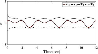
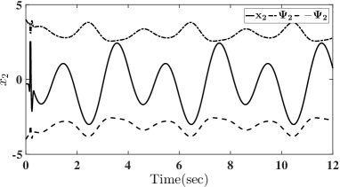
Figure 1: Output tracking and boundedness performance of $x_{1}$.

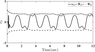
Figure 2: Boundedness performance and trajectory of the state variable $x_{2}$.

Figure 3: Boundedness performance and trajectory of the state variable $x_{3}$.

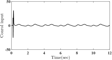
Figure 4: The control input signal.

V Simulation Results and discussion

Consider a third-order pure feedback nonlinear system [6]

$$\begin{split}\dot{x}_{1}&=x_{2}+0.05\cos(x_{1})+d_{1}\\ \dot{x}_{2}&=\frac{1-2^{x_{1}x_{2}}}{1+2^{x_{1}^{2}}}+x_{3}+0.1\tanh(x_{3})+d_{2}\\ \dot{x}_{3}&=0.2\times 3^{-x_{2}^{2}x_{3}^{4}}+(0.9+0.05\exp(-x_{1}^{2}))u\\ &\quad+0.2\cos(u)+d_{3}\\ y&=x_{1}\end{split}$$ (92)

where $x_{1},x_{2}$, and $x_{3}$ are the states, $u$ is the control input, and $y=x_{1}$ is the output of the system. To verify the robustness of proposed controller, disturbances $d_{1}=0.2\sin(\pi x_{1})$, $d_{2}=0.2\sin(\pi x_{1}x_{2})$, and $d_{3}=0.2x_{2}^{2}\sin(\pi x_{3})$ are considered in the system. Let, $y_{d}=0.5\cos(\pi t)+0.5\sin(0.5\pi t)$ be the system desired output of system, and $\Psi_{1}=e^{-0.2x_{1}}+e^{-3t}$, $\Psi_{2}=e^{-0.2x_{2}}+e^{-3t}+2\cos(0.5x_{1})$, and $\Psi_{3}=e^{-3t}+2\cos(0.5x_{1})$ be the constraints on system states $x_{1},x_{2}$, and $x_{3}$, respectively. The control objective is to design a control input $u$ such that the system output tracks the desired output $y_{d}$ and the system states do not contravene their respective constraints, i.e. $\mathinner{\!\left\lvert x_{1}\right\rvert}<\Psi_{1}$, $\mathinner{\!\left\lvert x_{2}\right\rvert}<\Psi_{2}$, and $\mathinner{\!\left\lvert x_{3}\right\rvert}<\Psi_{3}$.
Remark 8: It is given in [47] that any SISO system can be expressed in the form of (1).
We have designed an adaptive controller based on Table II. Table III has been used to update its parameters. The design parameter and initial values used in the simulation are: $k_{1}=k_{2}=k_{3}=7$; $k_{\varepsilon_{1}}=k_{\varepsilon_{2}}=k_{\varepsilon_{3}}=6$; $A_{0}=1$, $A_{1}=2$, $A_{2}=2$; $x_{1}(0)=0.5$, $x_{2}(0)=-0.3$, $x_{3}(0)=0$; $\lambda_{1}=\lambda_{2}=\lambda_{3}=10$, and $\zeta_{1}(0)=0$, $\zeta_{2}(0)=0$, $\zeta_{3}(0)=0.2$. The weights of the RBF NN are chosen as a $30\times 1$ dimensional vector, where 30 and 1 represent the number of nodes in the hidden layer and the output of the NN, respectively.

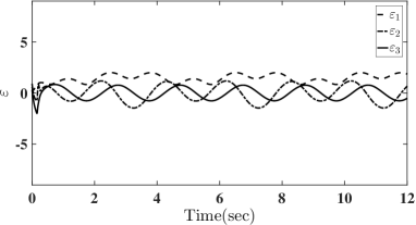
Figure 5: Trajectory of $\varepsilon_{1}$, $\varepsilon_{2}$, and $\varepsilon_{3}$.

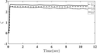
Figure 6: Trajectories of $\zeta_{1}$,$\zeta_{2}$, and $\zeta_{3}$.

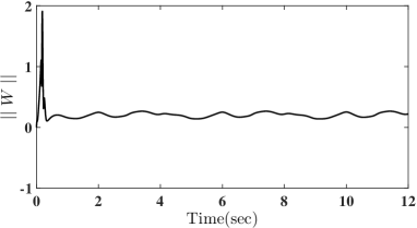
Figure 7: Norm of NN weights $W_{1}$, $W_{2}$, and $W_{3}$.

The simulation results are shown in Figs. 3-7; Figs. 3-3 show the trajectories of the states and their symmetric time-varying and state-dependent constraints. From Figs. 3-3 we can see that all the states are bounded in nature and doesn’t contravene their respective constraints. Also, from Fig. 3 it can be seen that the output tracks its desired trajectory satisfactorily. Furthermore, as proved in Theorem 1, it can be seen from Figs. 3-7 that all the signals in the closed-loop system, i.e. control input $u_{1}$ in Fig. 4, disturbance observer variables $\varepsilon_{1}$, $\varepsilon_{2}$, and $\varepsilon_{3}$ in Fig. 5, Nussbaum gain parameter $\zeta_{1},\zeta_{2}$, and $\zeta_{3}$ in Fig. 6, and Norm of NN weights matrix $W_{1}$, $W_{2}$, and $W_{3}$ in Fig. 7 are bounded in nature. The result thus shows the effectiveness of the proposed methodology.

VI Conclusion

A robust adaptive backstepping control is proposed for the tracking control of a pure feedback nonlinear system with symmetric SVICs on the state variables. The proposed controller doesn’t require prior knowledge of the system dynamics. The neural network is introduced to approximate the behaviour of unknown dynamics which arise during the time derivative of BLF. The use of disturbance observer helped much in making the controller robust and computationally inexpensive by estimating the disturbance along with NN approximation error and derivative of virtual control input. Through the simulation study, it is shown that all the signals in the closed-loop system are bounded and do not contravene their constraints. In future, this work can be extended for a stochastic pure feedback nonlinear system with asymmetric SVICs on the state variables.

References

- [1] K. P. Tee, S. S. Ge, and E. H. Tay, “Barrier lyapunov functions for the control of output-constrained nonlinear systems,” Automatica, vol. 45, no. 4, pp. 918 – 927, 2009.
- [2] K. P. Tee, B. Ren, and S. S. Ge, “Control of nonlinear systems with time-varying output constraints,” Automatica, vol. 47, no. 11, pp. 2511 – 2516, 2011.
- [3] B. Ren, S. S. Ge, K. P. Tee, and T. H. Lee, “Adaptive neural control for output feedback nonlinear systems using a barrier lyapunov function,” IEEE Trans. Neural Netw., vol. 21, pp. 1339–1345, Aug 2010.
- [4] W. He, S. Zhang, and S. S. Ge, “Adaptive control of a flexible crane system with the boundary output constraint,” IEEE Trans. Ind. Electron., vol. 61, pp. 4126–4133, Aug 2014.
- [5] K. P. Tee, S. S. Ge, and F. E. H. Tay, “Adaptive control of electrostatic microactuators with bidirectional drive,” IEEE Trans. Control Syst. Technol., vol. 17, pp. 340–352, March 2009.
- [6] W. Meng, Q. Yang, J. Si, and Y. Sun, “Adaptive neural control of a class of output-constrained nonaffine systems,” IEEE Trans. Cybern., vol. 46, pp. 85–95, Jan 2016.
- [7] K. P. Tee and S. S. Ge, “Control of nonlinear systems with partial state constraints using a barrier lyapunov function,” International Journal of Control, vol. 84, no. 12, pp. 2008–2023, 2011.
- [8] Y. J. Liu, J. Li, S. Tong, and C. L. P. Chen, “Neural network control-based adaptive learning design for nonlinear systems with full-state constraints,” IEEE Trans. Neural Netw. Learn. Syst., vol. 27, pp. 1562–1571, July 2016.
- [9] Y.-J. Liu and S. Tong, “Barrier lyapunov functions-based adaptive control for a class of nonlinear pure-feedback systems with full state constraints,” Automatica, vol. 64, pp. 70 – 75, 2016.
- [10] Y. J. Liu and S. Tong, “Barrier lyapunov functions for nussbaum gain adaptive control of full state constrained nonlinear systems,” Automatica, vol. 76, pp. 143 – 152, 2017.
- [11] Y. J. Liu, S. Tong, C. L. P. Chen, and D. J. Li, “Adaptive nn control using integral barrier lyapunov functionals for uncertain nonlinear block-triangular constraint systems,” IEEE Trans. Cybern., vol. 47, pp. 3747–3757, Nov 2017.
- [12] Z. Chen, Z. Li, and C. L. P. Chen, “Adaptive neural control of uncertain mimo nonlinear systems with state and input constraints,” IEEE Trans. Neural Netw. Learn. Syst., vol. 28, pp. 1318–1330, June 2017.
- [13] Y. J. Liu, S. Lu, D. Li, and S. Tong, “Adaptive controller design-based ablf for a class of nonlinear time-varying state constraint systems,” IEEE Trans. Syst., Man, and Cybern.: Syst., vol. 47, pp. 1546–1553, July 2017.
- [14] P. K. Mishra, N. K. Dhar, and N. K. Verma, “Adaptive neural-network control of mimo nonaffine nonlinear systems with asymmetric time-varying state constraints,” IEEE Trans. Cybern., pp. 1–13, 2019.
- [15] Y. Liu, M. Gong, L. Liu, S. Tong, and C. L. P. Chen, “Fuzzy observer constraint based on adaptive control for uncertain nonlinear mimo systems with time-varying state constraints,” IEEE Trans. Cybern., pp. 1–10, 2019.
- [16] C. P. Bechlioulis and G. A. Rovithakis, “Robust adaptive control of feedback linearizable mimo nonlinear systems with prescribed performance,” IEEE Trans. Autom. Control, vol. 53, pp. 2090–2099, Oct 2008.
- [17] C. P. Bechlioulis and G. A. Rovithakis, “Adaptive control with guaranteed transient and steady state tracking error bounds for strict feedback systems,” Automatica, vol. 45, no. 2, pp. 532 – 538, 2009.
- [18] W. Wang and C. Wen, “Adaptive actuator failure compensation control of uncertain nonlinear systems with guaranteed transient performance,” Automatica, vol. 46, no. 12, pp. 2082 – 2091, 2010.
- [19] C. P. Bechlioulis and G. A. Rovithakis, “Robust partial-state feedback prescribed performance control of cascade systems with unknown nonlinearities,” IEEE Trans. Autom. Control, vol. 56, pp. 2224–2230, Sep. 2011.
- [20] C. P. Bechlioulis and G. A. Rovithakis, “A low-complexity global approximation-free control scheme with prescribed performance for unknown pure feedback systems,” Automatica, vol. 50, no. 4, pp. 1217 – 1226, 2014.
- [21] D. Mayne, J. Rawlings, C. Rao, and P. Scokaert, “Constrained model predictive control: Stability and optimality,” Automatica, vol. 36, no. 6, pp. 789 – 814, 2000.
- [22] D. E. Kirk, Optimal Control Theory: An Introduction. Dover, 2016.
- [23] T. Gao, Y. Liu, L. Liu, and D. Li, “Adaptive neural network-based control for a class of nonlinear pure-feedback systems with time-varying full state constraints,” IEEE/CAA Journal of Automatica Sinica, vol. 5, pp. 923–933, Sep. 2018.
- [24] Y. Cao, Y. Song, and C. Wen, “Practical tracking control of perturbed uncertain nonaffine systems with full state constraints,” Automatica, vol. 110, p. 108608, 2019.
- [25] Y. Hua and T. Zhang, “Adaptive control of pure-feedback nonlinear systems with full-state time-varying constraints and unmodeled dynamics,” Int. J. of Adaptive Control and Signal Process., vol. 34, no. 2, pp. 183–198, 2020.
- [26] R. Hartl, S. Sethi, and R. Vickson, “A survey of the maximum principles for optimal control problems with state constraints,” SIAM Review, vol. 37, no. 2, pp. 181–218, 1995.
- [27] S. S. Ge and J. Wang, “Robust adaptive tracking for time-varying uncertain nonlinear systems with unknown control coefficients,” IEEE Trans. Autom. Control, vol. 48, pp. 1463–1469, Aug 2003.
- [28] H. E. Psillakis, “Further results on the use of nussbaum gains in adaptive neural network control,” IEEE Trans. Autom. Control, vol. 55, pp. 2841–2846, Dec 2010.
- [29] C. Wen, J. Zhou, Z. Liu, and H. Su, “Robust adaptive control of uncertain nonlinear systems in the presence of input saturation and external disturbance,” IEEE Trans. Autom. Control, vol. 56, pp. 1672–1678, July 2011.
- [30] Y. Liu, L. Ma, L. Liu, S. Tong, and C. L. P. Chen, “Adaptive neural network learning controller design for a class of nonlinear systems with time-varying state constraints,” IEEE Trans. Neural Netw. Learn. Syst., pp. 1–10, 2019.
- [31] B. Cui, Y. Xia, K. Liu, and G. Shen, “Finite-time tracking control for a class of uncertain strict-feedback nonlinear systems with state constraints: A smooth control approach,” IEEE Trans. Neural Netw. Learn. Syst., pp. 1–13, 2020.
- [32] D. Li and D. Li, “Adaptive tracking control for nonlinear time-varying delay systems with full state constraints and unknown control coefficients,” Automatica, vol. 93, pp. 444 – 453, 2018.
- [33] X. Huang, Y. Song, and J. Lai, “Neuro-adaptive control with given performance specifications for strict feedback systems under full-state constraints,” IEEE Trans. Neural Netw. Learn. Syst., vol. 30, pp. 25–34, Jan 2019.
- [34] D. Li, Y. Liu, S. Tong, C. L. P. Chen, and D. Li, “Neural networks-based adaptive control for nonlinear state constrained systems with input delay,” IEEE Trans. Cybern., vol. 49, pp. 1249–1258, April 2019.
- [35] J. Qiu, K. Sun, I. J. Rudas, and H. Gao, “Command filter-based adaptive nn control for mimo nonlinear systems with full-state constraints and actuator hysteresis,” IEEE Trans. Cybern., pp. 1–11, 2019.
- [36] R. Q. Fuentes-Aguilar and I. Chairez, “Adaptive tracking control of state constraint systems based on differential neural networks: A barrier lyapunov function approach,” IEEE Trans. Neural Netw. Learn. Syst., pp. 1–12, 2020.
- [37] M. Wang, Y. Zou, and C. Yang, “System transformation-based neural control for full-state-constrained pure-feedback systems via disturbance observer,” IEEE Trans. Cybern., pp. 1–11, 2020.
- [38] T. Wang, J. Wu, Y. Wang, and M. Ma, “Adaptive fuzzy tracking control for a class of strict-feedback nonlinear systems with time-varying input delay and full state constraints,” IEEE Trans. Fuzzy Syst., pp. 1–1, 2019.
- [39] K. Zhao and Y. Song, “Neuroadaptive robotic control under time-varying asymmetric motion constraints: A feasibility-condition-free approach,” IEEE Trans. Cybern., vol. 50, pp. 15–24, Jan 2020.
- [40] D. Li, S. Lu, and L. Liu, “Adaptive nn cross backstepping control for nonlinear systems with partial time-varying state constraints and its applications to hyper-chaotic systems,” IEEE Trans. Syst., Man, and Cybern.: Syst., pp. 1–12, 2019.
- [41] C. Xi and J. Dong, “Adaptive neural network-based control of uncertain nonlinear systems with time-varying full-state constraints and input constraint,” Neurocomputing, vol. 357, pp. 108 – 115, 2019.
- [42] Y.-D. Song and S. Zhou, “Tracking control of uncertain nonlinear systems with deferred asymmetric time-varying full state constraints,” Automatica, vol. 98, pp. 314 – 322, 2018.
- [43] Y. Sun, S. Gao, L. Ning, H. Dong, and B. Ning, “Output tracking control of strict-feedback non-linear systems under asymmetrically bilateral and time-varying full-state constraints,” IET Control Theory Applications, vol. 14, no. 1, pp. 156–164, 2020.
- [44] D. Li, C. L. P. Chen, Y. Liu, and S. Tong, “Neural network controller design for a class of nonlinear delayed systems with time-varying full-state constraints,” IEEE Trans. Neural Netw. Learn. Syst, vol. 30, pp. 2625–2636, Sep. 2019.
- [45] B. Xian and Y. Zhang, “Continuous asymptotically tracking control for a class of nonaffine-in-input system with nonvanishing disturbance,” IEEE Trans. Autom. Control, vol. 62, pp. 6019–6025, Nov 2017.
- [46] R. D. Nussbaum, “Some remarks on a conjecture in parameter adaptive control,” Systems and Control Letters, vol. 3, no. 5, pp. 243–246, 1983.
- [47] A. Zou, Z. Hou, and M. Tan, “Adaptive control of a class of nonlinear pure-feedback systems using fuzzy backstepping approach,” IEEE Trans. Fuzzy Syst., vol. 16, pp. 886–897, Aug 2008.