2 Bilocality of tripartite correlation tensors
In what follows, we use [ n ] delimited-[] 𝑛 [n] { 1 , 2 , … , n } 1 2 … 𝑛 \{1,2,\ldots,n\} A , B 𝐴 𝐵
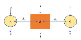
A,B C 𝐶 C x ∈ [ m A ] , y ∈ [ m B ] formulae-sequence 𝑥 delimited-[] subscript 𝑚 𝐴 𝑦 delimited-[] subscript 𝑚 𝐵 x\in[m_{A}],y\in[m_{B}] z ∈ [ m C ] 𝑧 delimited-[] subscript 𝑚 𝐶 z\in[m_{C}] P ( a b c | x y z ) 𝑃 conditional 𝑎 𝑏 𝑐 𝑥 𝑦 𝑧 P(abc|xyz) a ∈ [ o A ] , b ∈ [ o B ] formulae-sequence 𝑎 delimited-[] subscript 𝑜 𝐴 𝑏 delimited-[] subscript 𝑜 𝐵 a\in[o_{A}],b\in[o_{B}] c ∈ [ o C ] 𝑐 delimited-[] subscript 𝑜 𝐶 c\in[o_{C}] 𝐏 = P ( a b c | x y z ) 𝐏 𝑃 conditional 𝑎 𝑏 𝑐 𝑥 𝑦 𝑧 {\bf{P}}=\Lbrack P(abc|xyz)\Rbrack Δ 3 = [ o A ] × [ o B ] × [ o C ] × [ m A ] × [ m B ] × [ m C ] subscript Δ 3 delimited-[] subscript 𝑜 𝐴 delimited-[] subscript 𝑜 𝐵 delimited-[] subscript 𝑜 𝐶 delimited-[] subscript 𝑚 𝐴 delimited-[] subscript 𝑚 𝐵 delimited-[] subscript 𝑚 𝐶 \Delta_{3}=[o_{A}]\times[o_{B}]\times[o_{C}]\times[m_{A}]\times[m_{B}]\times[m_{C}] correlation tensor (CT) [46 ] , just like a matrix. Abstractly, a tripartite CT over Δ 3 subscript Δ 3 \Delta_{3} P : Δ 3 → ℝ : 𝑃 → subscript Δ 3 ℝ P:\Delta_{3}\rightarrow{\mathbb{R}}
P ( a b c | x y z ) ≥ 0 ( ∀ x , y , z , a , b , c ) and ∑ a , b , c P ( a b c | x y z ) = 1 ( ∀ x , y , z ) . 𝑃 conditional 𝑎 𝑏 𝑐 𝑥 𝑦 𝑧 0 for-all 𝑥 𝑦 𝑧 𝑎 𝑏 𝑐 and subscript 𝑎 𝑏 𝑐
𝑃 conditional 𝑎 𝑏 𝑐 𝑥 𝑦 𝑧 1 for-all 𝑥 𝑦 𝑧 P(abc|xyz)\geq 0(\forall x,y,z,a,b,c){\textrm{\ and\ }}\sum_{a,b,c}{P(abc|xyz)}=1(\forall x,y,z).
Any function P : Δ 3 → ℝ : 𝑃 → subscript Δ 3 ℝ P:\Delta_{3}\rightarrow{\mathbb{R}} correlation-type tensor (CTT)[46 ] over Δ 3 subscript Δ 3 \Delta_{3} 𝒯 ( Δ 3 ) 𝒯 subscript Δ 3 \mathcal{T}(\Delta_{3}) 𝒞 𝒯 ( Δ 3 ) 𝒞 𝒯 subscript Δ 3 \mathcal{CT}(\Delta_{3}) Δ 3 subscript Δ 3 \Delta_{3}
For any two elements 𝐏 = P ( a b c | x y z ) 𝐏 𝑃 conditional 𝑎 𝑏 𝑐 𝑥 𝑦 𝑧 {\bf{P}}=\Lbrack P(abc|xyz)\Rbrack 𝐐 = Q ( a b c | x y z ) 𝐐 𝑄 conditional 𝑎 𝑏 𝑐 𝑥 𝑦 𝑧 {\bf{Q}}=\Lbrack Q(abc|xyz)\Rbrack 𝒯 ( Δ 3 ) 𝒯 subscript Δ 3 \mathcal{T}(\Delta_{3})
s 𝐏 + t 𝐐 = s P ( a b c | x y z ) + t Q ( a b c | x y z ) , 𝑠 𝐏 𝑡 𝐐 𝑠 𝑃 conditional 𝑎 𝑏 𝑐 𝑥 𝑦 𝑧 𝑡 𝑄 conditional 𝑎 𝑏 𝑐 𝑥 𝑦 𝑧 s{\bf{P}}+t{\bf{Q}}=\Lbrack sP(abc|xyz)+tQ(abc|xyz)\Rbrack,
⟨ 𝐏 | 𝐐 ⟩ = ∑ a , b , c , x , y , z P ( a b c | x y z ) Q ( a b c | x y z ) , inner-product 𝐏 𝐐 subscript 𝑎 𝑏 𝑐 𝑥 𝑦 𝑧
𝑃 conditional 𝑎 𝑏 𝑐 𝑥 𝑦 𝑧 𝑄 conditional 𝑎 𝑏 𝑐 𝑥 𝑦 𝑧 \langle{\bf{P}}|{\bf{Q}}\rangle=\sum_{a,b,c,x,y,z}{P(abc|xyz)}Q(abc|xyz),
then 𝒯 ( Δ 3 ) 𝒯 subscript Δ 3 \mathcal{T}(\Delta_{3}) ℝ ℝ {\mathbb{R}} 𝒯 ( Δ 3 ) 𝒯 subscript Δ 3 \mathcal{T}(\Delta_{3}) 𝒞 𝒯 ( Δ 3 ) 𝒞 𝒯 subscript Δ 3 \mathcal{CT}(\Delta_{3}) 𝒯 ( Δ 3 ) 𝒯 subscript Δ 3 \mathcal{T}(\Delta_{3})
We fix the concept of the bilocality of a CT over Δ 3 subscript Δ 3 \Delta_{3} [30 , 31 ] .
Definition 2.1. A CT 𝐏 = P ( a b c | x y z ) 𝐏 𝑃 conditional 𝑎 𝑏 𝑐 𝑥 𝑦 𝑧 {\bf{P}}=\Lbrack P(abc|xyz)\Rbrack Δ 3 subscript Δ 3 \Delta_{3} bilocal if it has a “continuous” bilocal hidden variable model (C-biLHVM):
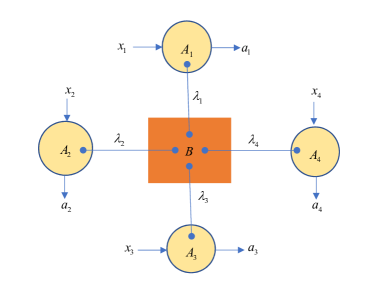
P ( a b c | x y z ) = ∬ Λ 1 × Λ 2 q 1 ( λ 1 ) q 2 ( λ 2 ) P A ( a | x , λ 1 ) P B ( b | y , λ 1 λ 2 ) P C ( c | z , λ 2 ) d μ 1 ( λ 1 ) d μ 2 ( λ 2 ) 𝑃 conditional 𝑎 𝑏 𝑐 𝑥 𝑦 𝑧 subscript double-integral subscript Λ 1 subscript Λ 2 subscript 𝑞 1 subscript 𝜆 1 subscript 𝑞 2 subscript 𝜆 2 subscript 𝑃 𝐴 conditional 𝑎 𝑥 subscript 𝜆 1
subscript 𝑃 𝐵 conditional 𝑏 𝑦 subscript 𝜆 1 subscript 𝜆 2
subscript 𝑃 𝐶 conditional 𝑐 𝑧 subscript 𝜆 2
differential-d subscript 𝜇 1 subscript 𝜆 1 differential-d subscript 𝜇 2 subscript 𝜆 2 P(abc|xyz)=\iint_{\Lambda_{1}\times\Lambda_{2}}q_{1}(\lambda_{1})q_{2}(\lambda_{2})P_{A}(a|x,\lambda_{1})P_{B}(b|y,\lambda_{1}\lambda_{2})P_{C}(c|z,\lambda_{2}){\rm{d}}\mu_{1}(\lambda_{1}){\rm{d}}\mu_{2}(\lambda_{2}) (2.1)
for a measure space ( Λ 1 × Λ 2 , Ω 1 × Ω 2 , μ 1 × μ 2 ) subscript Λ 1 subscript Λ 2 subscript Ω 1 subscript Ω 2 subscript 𝜇 1 subscript 𝜇 2 (\Lambda_{1}\times\Lambda_{2},\Omega_{1}\times\Omega_{2},\mu_{1}\times\mu_{2}) a , b , c , x , y , z 𝑎 𝑏 𝑐 𝑥 𝑦 𝑧
a,b,c,x,y,z
(a) q 1 ( λ 1 ) subscript 𝑞 1 subscript 𝜆 1 q_{1}(\lambda_{1}) P A ( a | x , λ 1 ) ( x ∈ [ m A ] , a ∈ [ o A ] ) subscript 𝑃 𝐴 conditional 𝑎 𝑥 subscript 𝜆 1
formulae-sequence 𝑥 delimited-[] subscript 𝑚 𝐴 𝑎 delimited-[] subscript 𝑜 𝐴 P_{A}(a|x,\lambda_{1})(x\in[m_{A}],a\in[o_{A}]) Ω 1 subscript Ω 1 \Omega_{1} Λ 1 subscript Λ 1 \Lambda_{1} q 2 ( λ 2 ) subscript 𝑞 2 subscript 𝜆 2 q_{2}(\lambda_{2}) P C ( c | z , λ 2 ) ( z ∈ [ m C ] , c ∈ [ o C ] ) subscript 𝑃 𝐶 conditional 𝑐 𝑧 subscript 𝜆 2
formulae-sequence 𝑧 delimited-[] subscript 𝑚 𝐶 𝑐 delimited-[] subscript 𝑜 𝐶 P_{C}(c|z,\lambda_{2})(z\in[m_{C}],c\in[o_{C}]) Ω 2 subscript Ω 2 \Omega_{2} Λ 2 subscript Λ 2 \Lambda_{2} P B ( b | y , λ 1 λ 2 ) ( y ∈ [ m B ] , b ∈ [ o B ] ) subscript 𝑃 𝐵 conditional 𝑏 𝑦 subscript 𝜆 1 subscript 𝜆 2
formulae-sequence 𝑦 delimited-[] subscript 𝑚 𝐵 𝑏 delimited-[] subscript 𝑜 𝐵 P_{B}(b|y,\lambda_{1}\lambda_{2})(y\in[m_{B}],b\in[o_{B}]) Ω 1 × Ω 2 subscript Ω 1 subscript Ω 2 \Omega_{1}\times\Omega_{2} Λ 1 × Λ 2 subscript Λ 1 subscript Λ 2 \Lambda_{1}\times\Lambda_{2}
(b) q i ( λ i ) , P A ( a | x , λ 1 ) , P B ( b | y , λ 1 λ 2 ) subscript 𝑞 𝑖 subscript 𝜆 𝑖 subscript 𝑃 𝐴 conditional 𝑎 𝑥 subscript 𝜆 1
subscript 𝑃 𝐵 conditional 𝑏 𝑦 subscript 𝜆 1 subscript 𝜆 2
q_{i}(\lambda_{i}),P_{A}(a|x,\lambda_{1}),P_{B}(b|y,\lambda_{1}\lambda_{2}) P C ( c | z , λ 2 ) subscript 𝑃 𝐶 conditional 𝑐 𝑧 subscript 𝜆 2
P_{C}(c|z,\lambda_{2}) λ i , a , b , c , subscript 𝜆 𝑖 𝑎 𝑏 𝑐
\lambda_{i},a,b,c,
A CT 𝐏 = P ( a b c | x y z ) 𝐏 𝑃 conditional 𝑎 𝑏 𝑐 𝑥 𝑦 𝑧 {\bf{P}}=\Lbrack P(abc|xyz)\Rbrack Δ 3 subscript Δ 3 \Delta_{3} non-bilocal if it is not bilocal. We use 𝒞 𝒯 bilocal ( Δ 3 ) 𝒞 superscript 𝒯 bilocal subscript Δ 3 \mathcal{CT}^{\textrm{bilocal}}(\Delta_{3}) Δ 3 subscript Δ 3 \Delta_{3}
Remark 2.1. By Definition 2.1, when a CT 𝐏 = P ( a b c | x y z ) 𝐏 𝑃 conditional 𝑎 𝑏 𝑐 𝑥 𝑦 𝑧 {\bf{P}}=\Lbrack P(abc|xyz)\Rbrack Δ 3 subscript Δ 3 \Delta_{3} P A ( a | x ) , P B ( b | y ) subscript 𝑃 𝐴 conditional 𝑎 𝑥 subscript 𝑃 𝐵 conditional 𝑏 𝑦
P_{A}(a|x),P_{B}(b|y) P C ( c | z ) subscript 𝑃 𝐶 conditional 𝑐 𝑧 P_{C}(c|z) A , B 𝐴 𝐵
A,B C 𝐶 C P ( a b c | x y z ) = P A ( a | x ) P B ( b | y ) P C ( c | z ) 𝑃 conditional 𝑎 𝑏 𝑐 𝑥 𝑦 𝑧 subscript 𝑃 𝐴 conditional 𝑎 𝑥 subscript 𝑃 𝐵 conditional 𝑏 𝑦 subscript 𝑃 𝐶 conditional 𝑐 𝑧 P(abc|xyz)=P_{A}(a|x)P_{B}(b|y)P_{C}(c|z)
P ( a b c | x y z ) = ∑ λ 1 λ 2 = 1 1 q 1 ( λ 1 ) q 2 ( λ 2 ) P A ( a | x , λ 1 ) P B ( b | y , λ 1 λ 2 ) P C ( c | z , λ 2 ) 𝑃 conditional 𝑎 𝑏 𝑐 𝑥 𝑦 𝑧 superscript subscript subscript 𝜆 1 subscript 𝜆 2 1 1 subscript 𝑞 1 subscript 𝜆 1 subscript 𝑞 2 subscript 𝜆 2 subscript 𝑃 𝐴 conditional 𝑎 𝑥 subscript 𝜆 1
subscript 𝑃 𝐵 conditional 𝑏 𝑦 subscript 𝜆 1 subscript 𝜆 2
subscript 𝑃 𝐶 conditional 𝑐 𝑧 subscript 𝜆 2
P(abc|xyz)=\sum_{\lambda_{1}\lambda_{2}=1}^{1}q_{1}(\lambda_{1})q_{2}(\lambda_{2})P_{A}(a|x,\lambda_{1})P_{B}(b|y,\lambda_{1}\lambda_{2})P_{C}(c|z,\lambda_{2})
where q k ( λ k ) = 1 ( k = 1 , 2 ) subscript 𝑞 𝑘 subscript 𝜆 𝑘 1 𝑘 1 2
q_{k}(\lambda_{k})=1(k=1,2)
P A ( a | x , λ 1 ) = P A ( a | x ) , P B ( b | y , λ 1 λ 2 ) = P B ( b | y ) , P C ( c | z , λ 2 ) = P C ( c | z ) , ∀ λ k = 1 . formulae-sequence subscript 𝑃 𝐴 conditional 𝑎 𝑥 subscript 𝜆 1
subscript 𝑃 𝐴 conditional 𝑎 𝑥 formulae-sequence subscript 𝑃 𝐵 conditional 𝑏 𝑦 subscript 𝜆 1 subscript 𝜆 2
subscript 𝑃 𝐵 conditional 𝑏 𝑦 formulae-sequence subscript 𝑃 𝐶 conditional 𝑐 𝑧 subscript 𝜆 2
subscript 𝑃 𝐶 conditional 𝑐 𝑧 for-all subscript 𝜆 𝑘 1 P_{A}(a|x,\lambda_{1})=P_{A}(a|x),P_{B}(b|y,\lambda_{1}\lambda_{2})=P_{B}(b|y),P_{C}(c|z,\lambda_{2})=P_{C}(c|z),\ \forall\lambda_{k}=1.
Thus, 𝐏 = P ( a b c | x y z ) 𝐏 𝑃 conditional 𝑎 𝑏 𝑐 𝑥 𝑦 𝑧 {\bf{P}}=\Lbrack P(abc|xyz)\Rbrack 2.1 μ k subscript 𝜇 𝑘 \mu_{k} Λ k = { 1 } subscript Λ 𝑘 1 \Lambda_{k}=\{1\}
Remark 2.2. From definition, we observe that when a CT 𝐏 = P ( a b c | x y z ) 𝐏 𝑃 conditional 𝑎 𝑏 𝑐 𝑥 𝑦 𝑧 {\bf{P}}=\Lbrack P(abc|xyz)\Rbrack Δ 3 subscript Δ 3 \Delta_{3}
P A C ( a c | x z ) = P A ( a | x ) P C ( c | z ) , ∀ x , z , a , c . subscript 𝑃 𝐴 𝐶 conditional 𝑎 𝑐 𝑥 𝑧 subscript 𝑃 𝐴 conditional 𝑎 𝑥 subscript 𝑃 𝐶 conditional 𝑐 𝑧 for-all 𝑥 𝑧 𝑎 𝑐
P_{AC}(ac|xz)=P_{A}(a|x)P_{C}(c|z),\ \ \forall x,z,a,c. (2.2)
By using this property of a bilocal CT, we can find that not all Bell local CTs over Δ 3 subscript Δ 3 \Delta_{3}
Example 2.1. Let m X = o X = 2 ( X = A , B , C ) subscript 𝑚 𝑋 subscript 𝑜 𝑋 2 𝑋 𝐴 𝐵 𝐶
m_{X}=o_{X}=2(X=A,B,C)
P B ( 1 | 1 ) = 1 / 2 , P B ( 2 | 1 ) = 1 / 2 , P B ( 1 | 2 ) = 1 / 2 , P B ( 2 | 2 ) = 1 / 2 , formulae-sequence subscript 𝑃 𝐵 conditional 1 1 1 2 formulae-sequence subscript 𝑃 𝐵 conditional 2 1 1 2 formulae-sequence subscript 𝑃 𝐵 conditional 1 2 1 2 subscript 𝑃 𝐵 conditional 2 2 1 2 P_{B}(1|1)=1/2,P_{B}(2|1)=1/2,P_{B}(1|2)=1/2,P_{B}(2|2)=1/2,
P A ′ ( 1 | 1 ) = 1 , P A ′ ( 2 | 1 ) = 0 , P A ′ ( 1 | 2 ) = 1 , P A ′ ( 2 | 2 ) = 0 , formulae-sequence subscript superscript 𝑃 ′ 𝐴 conditional 1 1 1 formulae-sequence subscript superscript 𝑃 ′ 𝐴 conditional 2 1 0 formulae-sequence subscript superscript 𝑃 ′ 𝐴 conditional 1 2 1 subscript superscript 𝑃 ′ 𝐴 conditional 2 2 0 P^{\prime}_{A}(1|1)=1,P^{\prime}_{A}(2|1)=0,P^{\prime}_{A}(1|2)=1,P^{\prime}_{A}(2|2)=0,
P A ′′ ( 1 | 1 ) = 0 , P A ′′ ( 2 | 1 ) = 1 , P A ′′ ( 1 | 2 ) = 0 , P A ′′ ( 2 | 2 ) = 1 , formulae-sequence subscript superscript 𝑃 ′′ 𝐴 conditional 1 1 0 formulae-sequence subscript superscript 𝑃 ′′ 𝐴 conditional 2 1 1 formulae-sequence subscript superscript 𝑃 ′′ 𝐴 conditional 1 2 0 subscript superscript 𝑃 ′′ 𝐴 conditional 2 2 1 P^{\prime\prime}_{A}(1|1)=0,P^{\prime\prime}_{A}(2|1)=1,P^{\prime\prime}_{A}(1|2)=0,P^{\prime\prime}_{A}(2|2)=1,
P C ′ ( 1 | 1 ) = 1 , P C ′ ( 2 | 1 ) = 0 , P C ′ ( 1 | 2 ) = 0 , P C ′ ( 2 | 2 ) = 1 , formulae-sequence subscript superscript 𝑃 ′ 𝐶 conditional 1 1 1 formulae-sequence subscript superscript 𝑃 ′ 𝐶 conditional 2 1 0 formulae-sequence subscript superscript 𝑃 ′ 𝐶 conditional 1 2 0 subscript superscript 𝑃 ′ 𝐶 conditional 2 2 1 P^{\prime}_{C}(1|1)=1,P^{\prime}_{C}(2|1)=0,P^{\prime}_{C}(1|2)=0,P^{\prime}_{C}(2|2)=1,
P C ′′ ( 1 | 1 ) = 0 , P C ′′ ( 2 | 1 ) = 1 , P C ′′ ( 1 | 2 ) = 1 , P C ′′ ( 2 | 2 ) = 0 , formulae-sequence subscript superscript 𝑃 ′′ 𝐶 conditional 1 1 0 formulae-sequence subscript superscript 𝑃 ′′ 𝐶 conditional 2 1 1 formulae-sequence subscript superscript 𝑃 ′′ 𝐶 conditional 1 2 1 subscript superscript 𝑃 ′′ 𝐶 conditional 2 2 0 P^{\prime\prime}_{C}(1|1)=0,P^{\prime\prime}_{C}(2|1)=1,P^{\prime\prime}_{C}(1|2)=1,P^{\prime\prime}_{C}(2|2)=0,
and define
𝐏 = 1 2 𝐏 A ′ ⊗ 𝐏 B ⊗ 𝐏 C ′ + 1 2 𝐏 A ′′ ⊗ 𝐏 B ⊗ 𝐏 C ′′ , 𝐏 tensor-product 1 2 subscript superscript 𝐏 ′ 𝐴 subscript 𝐏 𝐵 subscript superscript 𝐏 ′ 𝐶 tensor-product 1 2 subscript superscript 𝐏 ′′ 𝐴 subscript 𝐏 𝐵 subscript superscript 𝐏 ′′ 𝐶 {\bf{P}}=\frac{1}{2}{\bf{P}}^{\prime}_{A}{\otimes}{\bf{P}}_{B}{\otimes}{\bf{P}}^{\prime}_{C}+\frac{1}{2}{\bf{P}}^{\prime\prime}_{A}{\otimes}{\bf{P}}_{B}{\otimes}{\bf{P}}^{\prime\prime}_{C},
that is,
P ( a b c | x y z ) = 1 2 P A ′ ( a | x ) P B ( b | y ) P C ′ ( c | z ) + 1 2 P A ′′ ( a | x ) P B ( b | y ) P C ′′ ( c | z ) . 𝑃 conditional 𝑎 𝑏 𝑐 𝑥 𝑦 𝑧 1 2 subscript superscript 𝑃 ′ 𝐴 conditional 𝑎 𝑥 subscript 𝑃 𝐵 conditional 𝑏 𝑦 subscript superscript 𝑃 ′ 𝐶 conditional 𝑐 𝑧 1 2 subscript superscript 𝑃 ′′ 𝐴 conditional 𝑎 𝑥 subscript 𝑃 𝐵 conditional 𝑏 𝑦 subscript superscript 𝑃 ′′ 𝐶 conditional 𝑐 𝑧 P(abc|xyz)=\frac{1}{2}P^{\prime}_{A}(a|x)P_{B}(b|y)P^{\prime}_{C}(c|z)+\frac{1}{2}P^{\prime\prime}_{A}(a|x)P_{B}(b|y)P^{\prime\prime}_{C}(c|z).
Clearly, 𝐏 = P ( a b c | x y z ) 𝐏 𝑃 conditional 𝑎 𝑏 𝑐 𝑥 𝑦 𝑧 {\bf{P}}=\Lbrack P(abc|xyz)\Rbrack
| P A C ( a c | x z ) − P A ( a | x ) P C ( c | z ) | = 1 4 | [ P A ′ ( a | x ) − P A ′′ ( a | x ) ] [ P C ′ ( c | z ) − P C ′′ ( c | z ) ] | ≡ 1 4 , |P_{AC}(ac|xz)-P_{A}(a|x)P_{C}(c|z)|=\frac{1}{4}|[P^{\prime}_{A}(a|x)-P^{\prime\prime}_{A}(a|x)][P^{\prime}_{C}(c|z)-P^{\prime\prime}_{C}(c|z)]|\equiv\frac{1}{4},
we see that
P A C ( a c | x z ) ≠ P A ( a | x ) P C ( c | z ) , ∀ x , z , a , c . subscript 𝑃 𝐴 𝐶 conditional 𝑎 𝑐 𝑥 𝑧 subscript 𝑃 𝐴 conditional 𝑎 𝑥 subscript 𝑃 𝐶 conditional 𝑐 𝑧 for-all 𝑥 𝑧 𝑎 𝑐
P_{AC}(ac|xz)\neq P_{A}(a|x)P_{C}(c|z),\ \ \forall x,z,a,c.
Thus, 𝐏 ∉ 𝒞 𝒯 bilocal ( Δ 3 ) 𝐏 𝒞 superscript 𝒯 bilocal subscript Δ 3 {\bf{P}}\notin\mathcal{CT}^{\textrm{bilocal}}(\Delta_{3}) 𝐏 A ′ ⊗ 𝐏 B ⊗ 𝐏 C ′ tensor-product subscript superscript 𝐏 ′ 𝐴 subscript 𝐏 𝐵 subscript superscript 𝐏 ′ 𝐶 {\bf{P}}^{\prime}_{A}{\otimes}{\bf{P}}_{B}{\otimes}{\bf{P}}^{\prime}_{C} 𝐏 A ′′ ⊗ 𝐏 B ⊗ 𝐏 C ′′ tensor-product subscript superscript 𝐏 ′′ 𝐴 subscript 𝐏 𝐵 subscript superscript 𝐏 ′′ 𝐶 {\bf{P}}^{\prime\prime}_{A}{\otimes}{\bf{P}}_{B}{\otimes}{\bf{P}}^{\prime\prime}_{C} 𝒞 𝒯 bilocal ( Δ 3 ) 𝒞 superscript 𝒯 bilocal subscript Δ 3 \mathcal{CT}^{\textrm{bilocal}}(\Delta_{3}) 𝒞 𝒯 bilocal ( Δ 3 ) 𝒞 superscript 𝒯 bilocal subscript Δ 3 \mathcal{CT}^{\textrm{bilocal}}(\Delta_{3}) 𝒯 ( Δ 3 ) 𝒯 subscript Δ 3 \mathcal{T}(\Delta_{3})
Generally, the five PDs in a C-biLHVM (2.1 𝐏 𝐏 {\bf{P}} 𝐏 𝐏 {\bf{P}} Δ 3 subscript Δ 3 \Delta_{3}
Proposition 2.1. Let 𝐏 = P ( a b c | x y z ) 𝐏 𝑃 conditional 𝑎 𝑏 𝑐 𝑥 𝑦 𝑧 {\bf{P}}=\Lbrack P(abc|xyz)\Rbrack 𝐏 ′ = P ′ ( a b c | x y z ) superscript 𝐏 ′ superscript 𝑃 ′ conditional 𝑎 𝑏 𝑐 𝑥 𝑦 𝑧 {\bf{P}}^{\prime}=\Lbrack P^{\prime}(abc|xyz)\Rbrack Δ 3 subscript Δ 3 \Delta_{3} ( S 1 × S 2 , T 1 × T 2 , γ 1 × γ 2 ) subscript 𝑆 1 subscript 𝑆 2 subscript 𝑇 1 subscript 𝑇 2 subscript 𝛾 1 subscript 𝛾 2 (S_{1}\times S_{2},T_{1}\times T_{2},\gamma_{1}\times\gamma_{2}) f k ( s k ) subscript 𝑓 𝑘 subscript 𝑠 𝑘 f_{k}(s_{k}) s k ( k = 1 , 2 ) subscript 𝑠 𝑘 𝑘 1 2
s_{k}(k=1,2)
P ( a b c | x y z ) 𝑃 conditional 𝑎 𝑏 𝑐 𝑥 𝑦 𝑧 \displaystyle P(abc|xyz) = \displaystyle= ∬ S 1 × S 2 f 1 ( s 1 ) f 2 ( s 2 ) P A ( a | x , s 1 ) subscript double-integral subscript 𝑆 1 subscript 𝑆 2 subscript 𝑓 1 subscript 𝑠 1 subscript 𝑓 2 subscript 𝑠 2 subscript 𝑃 𝐴 conditional 𝑎 𝑥 subscript 𝑠 1
\displaystyle\iint_{S_{1}\times S_{2}}f_{1}(s_{1})f_{2}(s_{2})P_{A}(a|x,s_{1}) (2.3)
× P B ( b | y , s 1 s 2 ) P C ( c | z , s 2 ) d γ 1 ( s 1 ) d γ 2 ( s 2 ) , absent subscript 𝑃 𝐵 conditional 𝑏 𝑦 subscript 𝑠 1 subscript 𝑠 2
subscript 𝑃 𝐶 conditional 𝑐 𝑧 subscript 𝑠 2
d subscript 𝛾 1 subscript 𝑠 1 d subscript 𝛾 2 subscript 𝑠 2 \displaystyle\times P_{B}(b|y,s_{1}s_{2})P_{C}(c|z,s_{2}){\rm{d}}\gamma_{1}(s_{1}){\rm{d}}\gamma_{2}(s_{2}),
P ′ ( a b c | x y z ) superscript 𝑃 ′ conditional 𝑎 𝑏 𝑐 𝑥 𝑦 𝑧 \displaystyle P^{\prime}(abc|xyz) = \displaystyle= ∬ S 1 × S 2 f 1 ( s 1 ) f 2 ( s 2 ) P A ′ ( a | x , s 1 ) subscript double-integral subscript 𝑆 1 subscript 𝑆 2 subscript 𝑓 1 subscript 𝑠 1 subscript 𝑓 2 subscript 𝑠 2 subscript superscript 𝑃 ′ 𝐴 conditional 𝑎 𝑥 subscript 𝑠 1
\displaystyle\iint_{S_{1}\times S_{2}}f_{1}(s_{1})f_{2}(s_{2})P^{\prime}_{A}(a|x,s_{1}) (2.4)
× P B ′ ( b | y , s 1 s 2 ) P C ′ ( c | z , s 2 ) d γ 1 ( s 1 ) d γ 2 ( s 2 ) absent superscript subscript 𝑃 𝐵 ′ conditional 𝑏 𝑦 subscript 𝑠 1 subscript 𝑠 2
superscript subscript 𝑃 𝐶 ′ conditional 𝑐 𝑧 subscript 𝑠 2
d subscript 𝛾 1 subscript 𝑠 1 d subscript 𝛾 2 subscript 𝑠 2 \displaystyle\times P_{B}^{\prime}(b|y,s_{1}s_{2})P_{C}^{\prime}(c|z,s_{2}){\rm{d}}\gamma_{1}(s_{1}){\rm{d}}\gamma_{2}(s_{2})
for all a , b , c , x , y , z . 𝑎 𝑏 𝑐 𝑥 𝑦 𝑧
a,b,c,x,y,z.
Proof. By definition, 𝐏 𝐏 {\bf{P}} 𝐏 ′ superscript 𝐏 ′ {\bf{P}}^{\prime}
P ( a b c | x y z ) 𝑃 conditional 𝑎 𝑏 𝑐 𝑥 𝑦 𝑧 \displaystyle P(abc|xyz) = \displaystyle= ∬ Λ 1 × Λ 2 q 1 ( λ 1 ) q 2 ( λ 2 ) P A ( a | x , λ 1 ) subscript double-integral subscript Λ 1 subscript Λ 2 subscript 𝑞 1 subscript 𝜆 1 subscript 𝑞 2 subscript 𝜆 2 subscript 𝑃 𝐴 conditional 𝑎 𝑥 subscript 𝜆 1
\displaystyle\iint_{\Lambda_{1}\times\Lambda_{2}}q_{1}(\lambda_{1})q_{2}(\lambda_{2})P_{A}(a|x,\lambda_{1}) (2.5)
× P B ( b | y , λ 1 λ 2 ) P C ( c | z , λ 2 ) d μ 1 ( λ 1 ) d μ 2 ( λ 2 ) absent subscript 𝑃 𝐵 conditional 𝑏 𝑦 subscript 𝜆 1 subscript 𝜆 2
subscript 𝑃 𝐶 conditional 𝑐 𝑧 subscript 𝜆 2
d subscript 𝜇 1 subscript 𝜆 1 d subscript 𝜇 2 subscript 𝜆 2 \displaystyle\times P_{B}(b|y,\lambda_{1}\lambda_{2})P_{C}(c|z,\lambda_{2}){\rm{d}}\mu_{1}(\lambda_{1}){\rm{d}}\mu_{2}(\lambda_{2})
P ′ ( a b c | x y z ) superscript 𝑃 ′ conditional 𝑎 𝑏 𝑐 𝑥 𝑦 𝑧 \displaystyle P^{\prime}(abc|xyz) = \displaystyle= ∬ Λ 1 ′ × Λ 2 ′ q 1 ′ ( λ 1 ′ ) q 2 ′ ( λ 2 ′ ) P A ′ ( a | x , λ 1 ′ ) subscript double-integral superscript subscript Λ 1 ′ superscript subscript Λ 2 ′ superscript subscript 𝑞 1 ′ superscript subscript 𝜆 1 ′ superscript subscript 𝑞 2 ′ superscript subscript 𝜆 2 ′ superscript subscript 𝑃 𝐴 ′ conditional 𝑎 𝑥 superscript subscript 𝜆 1 ′
\displaystyle\iint_{\Lambda_{1}^{\prime}\times\Lambda_{2}^{\prime}}q_{1}^{\prime}(\lambda_{1}^{\prime})q_{2}^{\prime}(\lambda_{2}^{\prime})P_{A}^{\prime}(a|x,\lambda_{1}^{\prime}) (2.6)
× P B ′ ( b | y , λ 1 ′ λ 2 ′ ) P C ′ ( c | z , λ 2 ′ ) d μ 1 ′ ( λ 1 ′ ) d μ 2 ′ ( λ 2 ′ ) , absent superscript subscript 𝑃 𝐵 ′ conditional 𝑏 𝑦 superscript subscript 𝜆 1 ′ superscript subscript 𝜆 2 ′
superscript subscript 𝑃 𝐶 ′ conditional 𝑐 𝑧 superscript subscript 𝜆 2 ′
d superscript subscript 𝜇 1 ′ superscript subscript 𝜆 1 ′ d superscript subscript 𝜇 2 ′ superscript subscript 𝜆 2 ′ \displaystyle\times P_{B}^{\prime}(b|y,\lambda_{1}^{\prime}\lambda_{2}^{\prime})P_{C}^{\prime}(c|z,\lambda_{2}^{\prime}){\rm{d}}\mu_{1}^{\prime}(\lambda_{1}^{\prime}){\rm{d}}\mu_{2}^{\prime}(\lambda_{2}^{\prime}),
for some product measure spaces ( Λ 1 × Λ 2 , Ω 1 × Ω 2 , μ 1 × μ 2 ) subscript Λ 1 subscript Λ 2 subscript Ω 1 subscript Ω 2 subscript 𝜇 1 subscript 𝜇 2 (\Lambda_{1}\times\Lambda_{2},\Omega_{1}\times\Omega_{2},\mu_{1}\times\mu_{2}) ( Λ 1 ′ × Λ 2 ′ , Ω 1 ′ × Ω 2 ′ , μ 1 ′ × μ 2 ′ ) . superscript subscript Λ 1 ′ superscript subscript Λ 2 ′ superscript subscript Ω 1 ′ superscript subscript Ω 2 ′ superscript subscript 𝜇 1 ′ superscript subscript 𝜇 2 ′ (\Lambda_{1}^{\prime}\times\Lambda_{2}^{\prime},\Omega_{1}^{\prime}\times\Omega_{2}^{\prime},\mu_{1}^{\prime}\times\mu_{2}^{\prime}).
S k = Λ k × Λ k ′ , T k = Ω k × Ω k ′ , γ k = μ k × μ k ′ , formulae-sequence subscript 𝑆 𝑘 subscript Λ 𝑘 superscript subscript Λ 𝑘 ′ formulae-sequence subscript 𝑇 𝑘 subscript Ω 𝑘 superscript subscript Ω 𝑘 ′ subscript 𝛾 𝑘 subscript 𝜇 𝑘 superscript subscript 𝜇 𝑘 ′ S_{k}=\Lambda_{k}\times\Lambda_{k}^{\prime},T_{k}=\Omega_{k}\times\Omega_{k}^{\prime},\gamma_{k}=\mu_{k}\times\mu_{k}^{\prime},
s k = ( λ k , λ k ′ ) , f k ( s k ) = q k ( λ k ) q k ′ ( λ k ′ ) formulae-sequence subscript 𝑠 𝑘 subscript 𝜆 𝑘 superscript subscript 𝜆 𝑘 ′ subscript 𝑓 𝑘 subscript 𝑠 𝑘 subscript 𝑞 𝑘 subscript 𝜆 𝑘 superscript subscript 𝑞 𝑘 ′ superscript subscript 𝜆 𝑘 ′ s_{k}=(\lambda_{k},\lambda_{k}^{\prime}),f_{k}(s_{k})=q_{k}(\lambda_{k})q_{k}^{\prime}(\lambda_{k}^{\prime})
for k = 1 , 2 𝑘 1 2
k=1,2 ( S 1 × S 2 , T 1 × T 2 , γ 1 × γ 2 ) subscript 𝑆 1 subscript 𝑆 2 subscript 𝑇 1 subscript 𝑇 2 subscript 𝛾 1 subscript 𝛾 2 (S_{1}\times S_{2},T_{1}\times T_{2},\gamma_{1}\times\gamma_{2}) s k subscript 𝑠 𝑘 s_{k} f k ( s k ) ( k = 1 , 2 ) subscript 𝑓 𝑘 subscript 𝑠 𝑘 𝑘 1 2
f_{k}(s_{k})(k=1,2)
P A ( a | x , s 1 ) = P A ( a | x , λ 1 ) , P B ( b | y , s 1 s 2 ) = P B ( b | y , λ 1 λ 2 ) , P C ( c | z , s 2 ) = P C ( c | z , λ 2 ) , formulae-sequence subscript 𝑃 𝐴 conditional 𝑎 𝑥 subscript 𝑠 1
subscript 𝑃 𝐴 conditional 𝑎 𝑥 subscript 𝜆 1
formulae-sequence subscript 𝑃 𝐵 conditional 𝑏 𝑦 subscript 𝑠 1 subscript 𝑠 2
subscript 𝑃 𝐵 conditional 𝑏 𝑦 subscript 𝜆 1 subscript 𝜆 2
subscript 𝑃 𝐶 conditional 𝑐 𝑧 subscript 𝑠 2
subscript 𝑃 𝐶 conditional 𝑐 𝑧 subscript 𝜆 2
P_{A}(a|x,s_{1})=P_{A}(a|x,\lambda_{1}),P_{B}(b|y,s_{1}s_{2})=P_{B}(b|y,\lambda_{1}\lambda_{2}),P_{C}(c|z,s_{2})=P_{C}(c|z,\lambda_{2}),
P A ′ ( a | x , s 1 ) = P A ′ ( a | x , λ 1 ′ ) , P B ′ ( b | y , s 1 s 2 ) = P B ′ ( b | y , λ 1 ′ λ 2 ′ ) , P C ′ ( c | z , s 2 ) = P C ′ ( c | z , λ 2 ′ ) , formulae-sequence superscript subscript 𝑃 𝐴 ′ conditional 𝑎 𝑥 subscript 𝑠 1
superscript subscript 𝑃 𝐴 ′ conditional 𝑎 𝑥 superscript subscript 𝜆 1 ′
formulae-sequence superscript subscript 𝑃 𝐵 ′ conditional 𝑏 𝑦 subscript 𝑠 1 subscript 𝑠 2
superscript subscript 𝑃 𝐵 ′ conditional 𝑏 𝑦 superscript subscript 𝜆 1 ′ superscript subscript 𝜆 2 ′
superscript subscript 𝑃 𝐶 ′ conditional 𝑐 𝑧 subscript 𝑠 2
superscript subscript 𝑃 𝐶 ′ conditional 𝑐 𝑧 superscript subscript 𝜆 2 ′
P_{A}^{\prime}(a|x,s_{1})=P_{A}^{\prime}(a|x,\lambda_{1}^{\prime}),P_{B}^{\prime}(b|y,s_{1}s_{2})=P_{B}^{\prime}(b|y,\lambda_{1}^{\prime}\lambda_{2}^{\prime}),P_{C}^{\prime}(c|z,s_{2})=P_{C}^{\prime}(c|z,\lambda_{2}^{\prime}),
for all s k = ( λ k , λ k ′ ) subscript 𝑠 𝑘 subscript 𝜆 𝑘 superscript subscript 𝜆 𝑘 ′ s_{k}=(\lambda_{k},\lambda_{k}^{\prime}) S k subscript 𝑆 𝑘 S_{k} 2.5
∬ S 1 × S 2 f 1 ( s 1 ) f 2 ( s 2 ) P A ( a | x , s 1 ) P B ( b | y , s 1 s 2 ) P C ( c | z , s 2 ) d γ 1 ( s 1 ) d γ 2 ( s 2 ) subscript double-integral subscript 𝑆 1 subscript 𝑆 2 subscript 𝑓 1 subscript 𝑠 1 subscript 𝑓 2 subscript 𝑠 2 subscript 𝑃 𝐴 conditional 𝑎 𝑥 subscript 𝑠 1
subscript 𝑃 𝐵 conditional 𝑏 𝑦 subscript 𝑠 1 subscript 𝑠 2
subscript 𝑃 𝐶 conditional 𝑐 𝑧 subscript 𝑠 2
differential-d subscript 𝛾 1 subscript 𝑠 1 differential-d subscript 𝛾 2 subscript 𝑠 2 \displaystyle\iint_{S_{1}\times S_{2}}f_{1}(s_{1})f_{2}(s_{2})P_{A}(a|x,s_{1})P_{B}(b|y,s_{1}s_{2})P_{C}(c|z,s_{2}){\rm{d}}\gamma_{1}(s_{1}){\rm{d}}\gamma_{2}(s_{2})
= \displaystyle= ∬ Λ 1 ′ × Λ 2 ′ q 1 ′ ( λ 1 ′ ) q 2 ′ ( λ 2 ′ ) d μ 1 ′ ( λ 1 ′ ) d μ 2 ′ ( λ 2 ′ ) subscript double-integral superscript subscript Λ 1 ′ superscript subscript Λ 2 ′ superscript subscript 𝑞 1 ′ superscript subscript 𝜆 1 ′ superscript subscript 𝑞 2 ′ superscript subscript 𝜆 2 ′ differential-d superscript subscript 𝜇 1 ′ superscript subscript 𝜆 1 ′ differential-d superscript subscript 𝜇 2 ′ superscript subscript 𝜆 2 ′ \displaystyle\iint_{\Lambda_{1}^{\prime}\times\Lambda_{2}^{\prime}}q_{1}^{\prime}(\lambda_{1}^{\prime})q_{2}^{\prime}(\lambda_{2}^{\prime}){\rm{d}}\mu_{1}^{\prime}(\lambda_{1}^{\prime}){\rm{d}}\mu_{2}^{\prime}(\lambda_{2}^{\prime})
× ∬ Λ 1 × Λ 2 q 1 ( λ 1 ) q 2 ( λ 2 ) P A ( a | x , λ 1 ) P B ( b | y , λ 1 λ 2 ) P C ( c | z , λ 2 ) d μ 1 ( λ 1 ) d μ 2 ( λ 2 ) \displaystyle\times\iint_{\Lambda_{1}\times\Lambda_{2}}q_{1}(\lambda_{1})q_{2}(\lambda_{2})P_{A}(a|x,\lambda_{1})P_{B}(b|y,\lambda_{1}\lambda_{2})P_{C}(c|z,\lambda_{2}){\rm{d}}\mu_{1}(\lambda_{1}){\rm{d}}\mu_{2}(\lambda_{2})
= \displaystyle= P ( a b c | x y z ) , 𝑃 conditional 𝑎 𝑏 𝑐 𝑥 𝑦 𝑧 \displaystyle P(abc|xyz),
leading to Eq. (2.3 2.4 2.6
Moreover, when a CT 𝐏 = P ( a b c | x y z ) 𝐏 𝑃 conditional 𝑎 𝑏 𝑐 𝑥 𝑦 𝑧 {\bf{P}}=\Lbrack P(abc|xyz)\Rbrack Δ 3 subscript Δ 3 \Delta_{3} 2.1 μ i subscript 𝜇 𝑖 \mu_{i} Λ i subscript Λ 𝑖 \Lambda_{i} i = 1 , 2 𝑖 1 2
i=1,2 2.1
P ( a b c | x y z ) = ∑ λ 1 = 1 d 1 ∑ λ 2 = 1 d 2 q 1 ( λ 1 ) q 2 ( λ 2 ) P A ( a | x , λ 1 ) P B ( b | y , λ 1 λ 2 ) P C ( c | z , λ 2 ) 𝑃 conditional 𝑎 𝑏 𝑐 𝑥 𝑦 𝑧 superscript subscript subscript 𝜆 1 1 subscript 𝑑 1 superscript subscript subscript 𝜆 2 1 subscript 𝑑 2 subscript 𝑞 1 subscript 𝜆 1 subscript 𝑞 2 subscript 𝜆 2 subscript 𝑃 𝐴 conditional 𝑎 𝑥 subscript 𝜆 1
subscript 𝑃 𝐵 conditional 𝑏 𝑦 subscript 𝜆 1 subscript 𝜆 2
subscript 𝑃 𝐶 conditional 𝑐 𝑧 subscript 𝜆 2
P(abc|xyz)=\sum_{\lambda_{1}=1}^{d_{1}}\sum_{\lambda_{2}=1}^{d_{2}}q_{1}(\lambda_{1})q_{2}(\lambda_{2})P_{A}(a|x,\lambda_{1})P_{B}(b|y,\lambda_{1}\lambda_{2})P_{C}(c|z,\lambda_{2}) (2.7)
where q i ( λ i ) , P A ( a | x , λ 1 ) , P B ( b | y , λ 1 λ 2 ) subscript 𝑞 𝑖 subscript 𝜆 𝑖 subscript 𝑃 𝐴 conditional 𝑎 𝑥 subscript 𝜆 1
subscript 𝑃 𝐵 conditional 𝑏 𝑦 subscript 𝜆 1 subscript 𝜆 2
q_{i}(\lambda_{i}),P_{A}(a|x,\lambda_{1}),P_{B}(b|y,\lambda_{1}\lambda_{2}) P C ( c | z , λ 2 ) subscript 𝑃 𝐶 conditional 𝑐 𝑧 subscript 𝜆 2
P_{C}(c|z,\lambda_{2})
Conversely, if a CT 𝐏 = P ( a b c | x y z ) 𝐏 𝑃 conditional 𝑎 𝑏 𝑐 𝑥 𝑦 𝑧 {\bf{P}}=\Lbrack P(abc|xyz)\Rbrack Δ 3 subscript Δ 3 \Delta_{3} 2.7 2.1 μ i subscript 𝜇 𝑖 \mu_{i} Λ i subscript Λ 𝑖 \Lambda_{i} i = 1 , 2 𝑖 1 2
i=1,2
To give our results, some notations are necessary.
Put N X = ( o X ) m X ( X = A , B , C ) subscript 𝑁 𝑋 superscript subscript 𝑜 𝑋 subscript 𝑚 𝑋 𝑋 𝐴 𝐵 𝐶
N_{X}=(o_{X})^{m_{X}}(X=A,B,C) [ m X ] delimited-[] subscript 𝑚 𝑋 [m_{X}] [ o X ] delimited-[] subscript 𝑜 𝑋 [o_{X}]
Ω A = { J 1 , J 2 , … , J N A } = { J | J : [ m A ] → [ o A ] } , subscript Ω 𝐴 subscript 𝐽 1 subscript 𝐽 2 … subscript 𝐽 subscript 𝑁 𝐴 conditional-set 𝐽 : 𝐽 → delimited-[] subscript 𝑚 𝐴 delimited-[] subscript 𝑜 𝐴 \Omega_{A}=\{J_{1},J_{2},\ldots,J_{N_{A}}\}=\{J|J:[m_{A}]\rightarrow[o_{A}]\},
Ω B = { K 1 , K 2 , … , K N B } = { K | K : [ m B ] → [ o B ] } , subscript Ω 𝐵 subscript 𝐾 1 subscript 𝐾 2 … subscript 𝐾 subscript 𝑁 𝐵 conditional-set 𝐾 : 𝐾 → delimited-[] subscript 𝑚 𝐵 delimited-[] subscript 𝑜 𝐵 \Omega_{B}=\{K_{1},K_{2},\ldots,K_{N_{B}}\}=\{K|K:[m_{B}]\rightarrow[o_{B}]\},
Ω C = { L 1 , L 2 , … , L N C } = { L | L : [ m C ] → [ o C ] } . subscript Ω 𝐶 subscript 𝐿 1 subscript 𝐿 2 … subscript 𝐿 subscript 𝑁 𝐶 conditional-set 𝐿 : 𝐿 → delimited-[] subscript 𝑚 𝐶 delimited-[] subscript 𝑜 𝐶 \Omega_{C}=\{L_{1},L_{2},\ldots,L_{N_{C}}\}=\{L|L:[m_{C}]\rightarrow[o_{C}]\}.
It is clear that every m × n 𝑚 𝑛 m\times n { 0 , 1 } 0 1 \{0,1\} T = [ T i j ] 𝑇 delimited-[] subscript 𝑇 𝑖 𝑗 T=[T_{ij}] F : [ m ] → [ n ] : 𝐹 → delimited-[] 𝑚 delimited-[] 𝑛 F:[m]\rightarrow[n] T i j = δ j , F ( i ) subscript 𝑇 𝑖 𝑗 subscript 𝛿 𝑗 𝐹 𝑖
T_{ij}=\delta_{j,F(i)} { 0 , 1 } 0 1 \{0,1\} m A × o A subscript 𝑚 𝐴 subscript 𝑜 𝐴 m_{A}\times o_{A} m B × o B subscript 𝑚 𝐵 subscript 𝑜 𝐵 m_{B}\times o_{B} m C × o C subscript 𝑚 𝐶 subscript 𝑜 𝐶 m_{C}\times o_{C}
R S M m A × o A ( 0 , 1 ) = { R i := [ δ a , J i ( x ) ] x , a : i = 1 , 2 , … , N A } , 𝑅 𝑆 subscript superscript 𝑀 0 1 subscript 𝑚 𝐴 subscript 𝑜 𝐴 conditional-set assign subscript 𝑅 𝑖 subscript delimited-[] subscript 𝛿 𝑎 subscript 𝐽 𝑖 𝑥
𝑥 𝑎
𝑖 1 2 … subscript 𝑁 𝐴
RSM^{(0,1)}_{m_{A}\times o_{A}}=\{R_{i}:=[\delta_{a,J_{i}(x)}]_{x,a}:i=1,2,\ldots,N_{A}\},
R S M m B × o B ( 0 , 1 ) = { K j := [ δ b , K j ( y ) ] y , b : j = 1 , 2 , … , N B } , 𝑅 𝑆 subscript superscript 𝑀 0 1 subscript 𝑚 𝐵 subscript 𝑜 𝐵 conditional-set assign subscript 𝐾 𝑗 subscript delimited-[] subscript 𝛿 𝑏 subscript 𝐾 𝑗 𝑦
𝑦 𝑏
𝑗 1 2 … subscript 𝑁 𝐵
RSM^{(0,1)}_{m_{B}\times o_{B}}=\{K_{j}:=[\delta_{b,K_{j}(y)}]_{y,b}:j=1,2,\ldots,N_{B}\},
R S M m C × o C ( 0 , 1 ) = { L k := [ δ c , L k ( z ) ] z , c : k = 1 , 2 , … , N C } , 𝑅 𝑆 subscript superscript 𝑀 0 1 subscript 𝑚 𝐶 subscript 𝑜 𝐶 conditional-set assign subscript 𝐿 𝑘 subscript delimited-[] subscript 𝛿 𝑐 subscript 𝐿 𝑘 𝑧
𝑧 𝑐
𝑘 1 2 … subscript 𝑁 𝐶
RSM^{(0,1)}_{m_{C}\times o_{C}}=\{L_{k}:=[\delta_{c,L_{k}(z)}]_{z,c}:k=1,2,\ldots,N_{C}\},
respectively.
Definition 2.2. (1) An m × n 𝑚 𝑛 m\times n B = [ b i j ] 𝐵 delimited-[] subscript 𝑏 𝑖 𝑗 B=[b_{ij}] b i j ≥ 0 subscript 𝑏 𝑖 𝑗 0 b_{ij}\geq 0 i , j 𝑖 𝑗
i,j ∑ j = 1 n b i j ( λ ) = 1 superscript subscript 𝑗 1 𝑛 subscript 𝑏 𝑖 𝑗 𝜆 1 \sum_{j=1}^{n}b_{ij}(\lambda)=1 i ∈ [ m ] . 𝑖 delimited-[] 𝑚 i\in[m]. B = [ b i j ] 𝐵 delimited-[] subscript 𝑏 𝑖 𝑗 B=[b_{ij}] { 0 , 1 } 0 1 \{0,1\} i 𝑖 i J ( i ) 𝐽 𝑖 J(i) b i j = δ j , J ( i ) subscript 𝑏 𝑖 𝑗 subscript 𝛿 𝑗 𝐽 𝑖
b_{ij}=\delta_{j,J(i)} { R k : k ∈ [ n m ] } conditional-set subscript 𝑅 𝑘 𝑘 delimited-[] superscript 𝑛 𝑚 \{R_{k}:k\in[n^{m}]\} m × n 𝑚 𝑛 m\times n { 0 , 1 } 0 1 \{0,1\}
(2) An m × n 𝑚 𝑛 m\times n B ( λ ) = [ b i j ( λ ) ] 𝐵 𝜆 delimited-[] subscript 𝑏 𝑖 𝑗 𝜆 B(\lambda)=[b_{ij}(\lambda)] Λ Λ \Lambda λ ∈ Λ 𝜆 Λ \lambda\in\Lambda b i j ( λ ) ≥ 0 subscript 𝑏 𝑖 𝑗 𝜆 0 b_{ij}(\lambda)\geq 0 i , j 𝑖 𝑗
i,j ∑ j = 1 n b i j ( λ ) = 1 superscript subscript 𝑗 1 𝑛 subscript 𝑏 𝑖 𝑗 𝜆 1 \sum_{j=1}^{n}b_{ij}(\lambda)=1 i ∈ [ m ] . 𝑖 delimited-[] 𝑚 i\in[m].
Recall that a measurable space (MS) [44 ] is a pair ( Λ , Ω ) Λ Ω (\Lambda,\Omega) Λ Λ \Lambda σ 𝜎 \sigma Ω Ω \Omega Λ Λ \Lambda ( Λ , Ω ) Λ Ω (\Lambda,\Omega) Ω Ω \Omega Ω Ω \Omega -measurable sets of Λ Λ \Lambda f : Λ → ℝ : 𝑓 → Λ ℝ f:\Lambda\rightarrow{\mathbb{R}} Ω Ω \Omega -measurable (measurable for short) if the inverse image f − 1 ( G ) superscript 𝑓 1 𝐺 f^{-1}(G) G 𝐺 G ℝ ℝ {\mathbb{R}} Ω Ω \Omega Ω Ω \Omega measure μ 𝜇 \mu Ω Ω \Omega Ω Ω \Omega
A i ∈ Ω ( i = 1 , 2 , … ) , A i ∩ A j = Ø ( i ≠ j ) ⇒ μ ( ⋃ i = 1 ∞ A i ) = ∑ i = 1 ∞ μ ( A i ) . formulae-sequence subscript 𝐴 𝑖 Ω 𝑖 1 2 …
subscript 𝐴 𝑖 subscript 𝐴 𝑗 italic-Ø 𝑖 𝑗 ⇒ 𝜇 superscript subscript 𝑖 1 subscript 𝐴 𝑖 superscript subscript 𝑖 1 𝜇 subscript 𝐴 𝑖 A_{i}\in\Omega(i=1,2,\ldots),A_{i}\cap A_{j}=\O(i\neq j)\Rightarrow\mu\left(\bigcup_{i=1}^{\infty}A_{i}\right)=\sum_{i=1}^{\infty}\mu(A_{i}).
Usually, we also assume that μ ( A ) < + ∞ 𝜇 𝐴 \mu(A)<+\infty A ∈ Ω 𝐴 Ω A\in\Omega measure space [44 ] means a triple ( Λ , Ω , μ ) Λ Ω 𝜇 (\Lambda,\Omega,\mu) Λ Λ \Lambda σ 𝜎 \sigma Ω Ω \Omega Λ Λ \Lambda μ 𝜇 \mu Ω Ω \Omega
Lemma 2.1. Let ( Λ , Ω ) Λ Ω (\Lambda,\Omega) m × n 𝑚 𝑛 m\times n B ( λ ) = [ b i j ( λ ) ] 𝐵 𝜆 delimited-[] subscript 𝑏 𝑖 𝑗 𝜆 B(\lambda)=[b_{ij}(\lambda)] Ω Ω \Omega Λ Λ \Lambda b i j subscript 𝑏 𝑖 𝑗 b_{ij} Ω Ω \Omega Λ Λ \Lambda B ( λ ) 𝐵 𝜆 B(\lambda)
B ( λ ) = ∑ k = 1 n m α k ( λ ) R k , ∀ λ ∈ Λ , formulae-sequence 𝐵 𝜆 superscript subscript 𝑘 1 superscript 𝑛 𝑚 subscript 𝛼 𝑘 𝜆 subscript 𝑅 𝑘 for-all 𝜆 Λ B(\lambda)=\sum_{k=1}^{n^{m}}\alpha_{k}(\lambda)R_{k},\ \forall\lambda\in\Lambda, (2.8)
where α k ( k = 1 , 2 , … , n m ) subscript 𝛼 𝑘 𝑘 1 2 … superscript 𝑛 𝑚
\alpha_{k}(k=1,2,\ldots,n^{m}) Ω Ω \Omega Λ Λ \Lambda ∑ k = 1 n m α k ( λ ) = 1 superscript subscript 𝑘 1 superscript 𝑛 𝑚 subscript 𝛼 𝑘 𝜆 1 \sum_{k=1}^{n^{m}}\alpha_{k}(\lambda)=1 λ ∈ Λ 𝜆 Λ \lambda\in\Lambda
The sufficiency is clear and the necessity is proved in Appendix.
Based on this lemma, we have the following theorem, which gives a series of equivalent characterizations of bilocality of a CT. Especially, it says that
a CT 𝐏 𝐏 {\bf{P}} Δ 3 subscript Δ 3 \Delta_{3} ( i i ) 𝑖 𝑖 (ii) [31 , Eq. (7)] by saying that “it is well known that Alice’s local response function P A ( a | x , λ 1 ) subscript 𝑃 𝐴 conditional 𝑎 𝑥 subscript 𝜆 1
P_{A}(a|x,\lambda_{1}) [18 ] . Indeed, Fine in [18 ] did not give a mathematical proof of this conclusion, just a physical description.
Theorem 2.1. Let 𝐏 = P ( a b c | x y z ) 𝐏 𝑃 conditional 𝑎 𝑏 𝑐 𝑥 𝑦 𝑧 {\bf{P}}=\Lbrack P(abc|xyz)\Rbrack Δ 3 subscript Δ 3 \Delta_{3} ( i ) 𝑖 (i) ( v ) 𝑣 (v)
(i) 𝐏 𝐏 {\bf{P}} 2.1
(ii) 𝐏 𝐏 {\bf{P}}
P ( a b c | x y z ) = ∑ i = 1 N A ∑ j = 1 N B ∑ k = 1 N C π ( i , j , k ) δ a , J i ( x ) δ b , K j ( y ) δ c , L k ( z ) , ∀ x , a , y , b , z , c , 𝑃 conditional 𝑎 𝑏 𝑐 𝑥 𝑦 𝑧 superscript subscript 𝑖 1 subscript 𝑁 𝐴 superscript subscript 𝑗 1 subscript 𝑁 𝐵 superscript subscript 𝑘 1 subscript 𝑁 𝐶 𝜋 𝑖 𝑗 𝑘 subscript 𝛿 𝑎 subscript 𝐽 𝑖 𝑥
subscript 𝛿 𝑏 subscript 𝐾 𝑗 𝑦
subscript 𝛿 𝑐 subscript 𝐿 𝑘 𝑧
for-all 𝑥 𝑎 𝑦 𝑏 𝑧 𝑐
P(abc|xyz)=\sum_{i=1}^{N_{A}}\sum_{j=1}^{N_{B}}\sum_{k=1}^{N_{C}}\pi({i,j,k})\delta_{a,J_{i}(x)}\delta_{b,K_{j}(y)}\delta_{c,L_{k}(z)},\ \forall x,a,y,b,z,c, (2.9)
where
π ( i , j , k ) = ∬ Λ 1 × Λ 2 q 1 ( λ 1 ) q 2 ( λ 2 ) α i ( λ 1 ) β j ( λ 1 λ 2 ) γ k ( λ 2 ) d μ 1 ( λ 1 ) d μ 2 ( λ 2 ) , 𝜋 𝑖 𝑗 𝑘 subscript double-integral subscript Λ 1 subscript Λ 2 subscript 𝑞 1 subscript 𝜆 1 subscript 𝑞 2 subscript 𝜆 2 subscript 𝛼 𝑖 subscript 𝜆 1 subscript 𝛽 𝑗 subscript 𝜆 1 subscript 𝜆 2 subscript 𝛾 𝑘 subscript 𝜆 2 differential-d subscript 𝜇 1 subscript 𝜆 1 differential-d subscript 𝜇 2 subscript 𝜆 2 \pi({i,j,k})=\iint_{\Lambda_{1}\times\Lambda_{2}}q_{1}(\lambda_{1})q_{2}(\lambda_{2})\alpha_{i}(\lambda_{1})\beta_{j}(\lambda_{1}\lambda_{2})\gamma_{k}(\lambda_{2}){\rm{d}}\mu_{1}(\lambda_{1}){\rm{d}}\mu_{2}(\lambda_{2}), (2.10)
q 1 ( λ 1 ) subscript 𝑞 1 subscript 𝜆 1 q_{1}(\lambda_{1}) and q 2 ( λ 2 ) subscript 𝑞 2 subscript 𝜆 2 q_{2}(\lambda_{2}) λ 1 subscript 𝜆 1 \lambda_{1} λ 2 subscript 𝜆 2 \lambda_{2} α i ( λ 1 ) subscript 𝛼 𝑖 subscript 𝜆 1 \alpha_{i}(\lambda_{1}) β j ( λ 1 λ 2 ) subscript 𝛽 𝑗 subscript 𝜆 1 subscript 𝜆 2 \beta_{j}(\lambda_{1}\lambda_{2}) γ k ( λ 2 ) subscript 𝛾 𝑘 subscript 𝜆 2 \gamma_{k}(\lambda_{2}) i , j 𝑖 𝑗
i,j k 𝑘 k λ 1 , ( λ 1 λ 2 ) subscript 𝜆 1 subscript 𝜆 1 subscript 𝜆 2
\lambda_{1},(\lambda_{1}\lambda_{2}) λ 2 subscript 𝜆 2 \lambda_{2}
(iii) 𝐏 𝐏 {\bf{P}}
P ( a b c | x y z ) = ∑ i = 1 N A ∑ k = 1 N C π 1 ( i ) π 2 ( k ) δ a , J i ( x ) P B ( b | y , i , k ) δ c , L k ( z ) , ∀ x , a , y , b , z , c , 𝑃 conditional 𝑎 𝑏 𝑐 𝑥 𝑦 𝑧 superscript subscript 𝑖 1 subscript 𝑁 𝐴 superscript subscript 𝑘 1 subscript 𝑁 𝐶 subscript 𝜋 1 𝑖 subscript 𝜋 2 𝑘 subscript 𝛿 𝑎 subscript 𝐽 𝑖 𝑥
subscript 𝑃 𝐵 conditional 𝑏 𝑦 𝑖 𝑘
subscript 𝛿 𝑐 subscript 𝐿 𝑘 𝑧
for-all 𝑥 𝑎 𝑦 𝑏 𝑧 𝑐
P(abc|xyz)=\sum_{i=1}^{N_{A}}\sum_{k=1}^{N_{C}}\pi_{1}(i)\pi_{2}(k)\delta_{a,J_{i}(x)}P_{B}(b|y,i,k)\delta_{c,L_{k}(z)},\ \forall x,a,y,b,z,c, (2.11)
where q i ( λ i ) , P A ( a | x , λ 1 ) , P B ( b | y , λ 1 λ 2 ) , P C ( c | z , λ 2 ) subscript 𝑞 𝑖 subscript 𝜆 𝑖 subscript 𝑃 𝐴 conditional 𝑎 𝑥 subscript 𝜆 1
subscript 𝑃 𝐵 conditional 𝑏 𝑦 subscript 𝜆 1 subscript 𝜆 2
subscript 𝑃 𝐶 conditional 𝑐 𝑧 subscript 𝜆 2
q_{i}(\lambda_{i}),P_{A}(a|x,\lambda_{1}),P_{B}(b|y,\lambda_{1}\lambda_{2}),P_{C}(c|z,\lambda_{2}) λ i , a , b , c , subscript 𝜆 𝑖 𝑎 𝑏 𝑐
\lambda_{i},a,b,c,
(iv) 𝐏 𝐏 {\bf{P}}
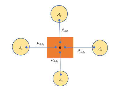
ℳ A B C = { M x y z } ( x , y , z ) ∈ [ m A ] × [ m B ] × [ m C ] subscript ℳ 𝐴 𝐵 𝐶 subscript superscript 𝑀 𝑥 𝑦 𝑧 𝑥 𝑦 𝑧 delimited-[] subscript 𝑚 𝐴 delimited-[] subscript 𝑚 𝐵 delimited-[] subscript 𝑚 𝐶 {\mathcal{M}}_{ABC}=\{M^{xyz}\}_{(x,y,z)\in[m_{A}]\times[m_{B}]\times[m_{C}]} (2.12)
of local POVMs M x y z = { M a | x ⊗ N b | y ⊗ L c | z } ( a , b , c ) ∈ [ o A ] × [ o B ] × [ o C ] superscript 𝑀 𝑥 𝑦 𝑧 subscript tensor-product subscript 𝑀 conditional 𝑎 𝑥 subscript 𝑁 conditional 𝑏 𝑦 subscript 𝐿 conditional 𝑐 𝑧 𝑎 𝑏 𝑐 delimited-[] subscript 𝑜 𝐴 delimited-[] subscript 𝑜 𝐵 delimited-[] subscript 𝑜 𝐶 M^{xyz}=\{M_{a|x}{\otimes}N_{b|y}{\otimes}L_{c|z}\}_{(a,b,c)\in[o_{A}]\times[o_{B}]\times[o_{C}]} ℋ A ⊗ ℋ B ⊗ ℋ C tensor-product subscript ℋ 𝐴 subscript ℋ 𝐵 subscript ℋ 𝐶 {\mathcal{H}}_{A}{\otimes}{\mathcal{H}}_{B}{\otimes}{\mathcal{H}}_{C} { ρ A B 1 , ρ B 2 C } subscript 𝜌 𝐴 subscript 𝐵 1 subscript 𝜌 subscript 𝐵 2 𝐶 \{\rho_{AB_{1}},\rho_{B_{2}C}\} ρ A B 1 subscript 𝜌 𝐴 subscript 𝐵 1 \rho_{AB_{1}} ρ B 2 C subscript 𝜌 subscript 𝐵 2 𝐶 \rho_{B_{2}C} ℋ A ⊗ ℋ B 1 tensor-product subscript ℋ 𝐴 subscript ℋ subscript 𝐵 1 {\mathcal{H}}_{A}{\otimes}{\mathcal{H}}_{B_{1}} ℋ B 2 ⊗ ℋ C tensor-product subscript ℋ subscript 𝐵 2 subscript ℋ 𝐶 {\mathcal{H}}_{B_{2}}{\otimes}{\mathcal{H}}_{C}
P ( a b c | x y z ) = tr [ ( M a | x ⊗ N b | y ⊗ L c | z ) ( ρ A B 1 ⊗ ρ B 2 C ) ] , ∀ x , a , y , b , z , c . 𝑃 conditional 𝑎 𝑏 𝑐 𝑥 𝑦 𝑧 tr delimited-[] tensor-product subscript 𝑀 conditional 𝑎 𝑥 subscript 𝑁 conditional 𝑏 𝑦 subscript 𝐿 conditional 𝑐 𝑧 tensor-product subscript 𝜌 𝐴 subscript 𝐵 1 subscript 𝜌 subscript 𝐵 2 𝐶 for-all 𝑥 𝑎 𝑦 𝑏 𝑧 𝑐
P(abc|xyz)={\rm{tr}}[(M_{a|x}{{\otimes}}N_{b|y}{\otimes}L_{c|z})(\rho_{AB_{1}}{\otimes}\rho_{B_{2}C})],\ \forall x,a,y,b,z,c. (2.13)
(v) 𝐏 𝐏 {\bf{P}}
P ( a b c | x y z ) = ∑ λ 1 = 1 d 1 ∑ λ 2 = 1 d 2 q 1 ( λ 1 ) q 2 ( λ 2 ) P A ( a | x , λ 1 ) P B ( b | y , λ 1 λ 2 ) P C ( c | z , λ 2 ) 𝑃 conditional 𝑎 𝑏 𝑐 𝑥 𝑦 𝑧 superscript subscript subscript 𝜆 1 1 subscript 𝑑 1 superscript subscript subscript 𝜆 2 1 subscript 𝑑 2 subscript 𝑞 1 subscript 𝜆 1 subscript 𝑞 2 subscript 𝜆 2 subscript 𝑃 𝐴 conditional 𝑎 𝑥 subscript 𝜆 1
subscript 𝑃 𝐵 conditional 𝑏 𝑦 subscript 𝜆 1 subscript 𝜆 2
subscript 𝑃 𝐶 conditional 𝑐 𝑧 subscript 𝜆 2
P(abc|xyz)=\sum_{\lambda_{1}=1}^{d_{1}}\sum_{\lambda_{2}=1}^{d_{2}}q_{1}(\lambda_{1})q_{2}(\lambda_{2})P_{A}(a|x,\lambda_{1})P_{B}(b|y,\lambda_{1}\lambda_{2})P_{C}(c|z,\lambda_{2}) (2.14)
where q i ( λ i ) , P A ( a | x , λ 1 ) , P B ( b | y , λ 1 λ 2 ) , P C ( c | z , λ 2 ) subscript 𝑞 𝑖 subscript 𝜆 𝑖 subscript 𝑃 𝐴 conditional 𝑎 𝑥 subscript 𝜆 1
subscript 𝑃 𝐵 conditional 𝑏 𝑦 subscript 𝜆 1 subscript 𝜆 2
subscript 𝑃 𝐶 conditional 𝑐 𝑧 subscript 𝜆 2
q_{i}(\lambda_{i}),P_{A}(a|x,\lambda_{1}),P_{B}(b|y,\lambda_{1}\lambda_{2}),P_{C}(c|z,\lambda_{2}) λ i , a , b , c , subscript 𝜆 𝑖 𝑎 𝑏 𝑐
\lambda_{i},a,b,c,
Proof. ( i ) ⇒ ( i i ) : : ⇒ 𝑖 𝑖 𝑖 absent (i)\Rightarrow(ii): ( i ) 𝑖 (i)
M 1 ( λ 1 ) := [ P A ( a | x , λ 1 ) ] x , a , M 2 ( λ 1 λ 2 ) := [ P B ( b | y , λ 1 λ 2 ) ] y , b , M 3 ( λ 2 ) = : [ P C ( c | z , λ 2 ) ] z , c M_{1}(\lambda_{1}):=[P_{A}(a|x,\lambda_{1})]_{x,a},M_{2}(\lambda_{1}\lambda_{2}):=[P_{B}(b|y,\lambda_{1}\lambda_{2})]_{y,b},M_{3}(\lambda_{2})=:[P_{C}(c|z,\lambda_{2})]_{z,c}
are RS matrices for each parameter λ k ∈ Λ k subscript 𝜆 𝑘 subscript Λ 𝑘 \lambda_{k}\in\Lambda_{k}
M 1 ( λ 1 ) = ∑ i = 1 N A α i ( λ 1 ) R i , subscript 𝑀 1 subscript 𝜆 1 superscript subscript 𝑖 1 subscript 𝑁 𝐴 subscript 𝛼 𝑖 subscript 𝜆 1 subscript 𝑅 𝑖 M_{1}(\lambda_{1})=\sum_{i=1}^{N_{A}}\alpha_{i}(\lambda_{1})R_{i},
M 2 ( λ 1 λ 2 ) = ∑ j = 1 N B β j ( λ 1 λ 2 ) Q j , subscript 𝑀 2 subscript 𝜆 1 subscript 𝜆 2 superscript subscript 𝑗 1 subscript 𝑁 𝐵 subscript 𝛽 𝑗 subscript 𝜆 1 subscript 𝜆 2 subscript 𝑄 𝑗 M_{2}(\lambda_{1}\lambda_{2})=\sum_{j=1}^{N_{B}}\beta_{j}(\lambda_{1}\lambda_{2})Q_{j},
M 3 ( λ 2 ) = ∑ k = 1 N C γ k ( λ 2 ) S k ; subscript 𝑀 3 subscript 𝜆 2 superscript subscript 𝑘 1 subscript 𝑁 𝐶 subscript 𝛾 𝑘 subscript 𝜆 2 subscript 𝑆 𝑘 M_{3}(\lambda_{2})=\sum_{k=1}^{N_{C}}\gamma_{k}(\lambda_{2})S_{k};
equivalently,
P ( a | x , λ ) = ∑ i = 1 N A α i ( λ 1 ) δ a , J i ( x ) , 𝑃 conditional 𝑎 𝑥 𝜆
superscript subscript 𝑖 1 subscript 𝑁 𝐴 subscript 𝛼 𝑖 subscript 𝜆 1 subscript 𝛿 𝑎 subscript 𝐽 𝑖 𝑥
P(a|x,\lambda)=\sum_{i=1}^{N_{A}}\alpha_{i}(\lambda_{1})\delta_{a,J_{i}(x)},
P ( b | y , λ 1 λ 2 ) = ∑ j = 1 N B β j ( λ 1 λ 2 ) δ b , K j ( y ) , 𝑃 conditional 𝑏 𝑦 subscript 𝜆 1 subscript 𝜆 2
superscript subscript 𝑗 1 subscript 𝑁 𝐵 subscript 𝛽 𝑗 subscript 𝜆 1 subscript 𝜆 2 subscript 𝛿 𝑏 subscript 𝐾 𝑗 𝑦
P(b|y,\lambda_{1}\lambda_{2})=\sum_{j=1}^{N_{B}}\beta_{j}(\lambda_{1}\lambda_{2})\delta_{b,K_{j}(y)},
P ( c | z , λ 2 ) = ∑ k = 1 N C γ k ( λ 2 ) δ c , L k ( z ) , 𝑃 conditional 𝑐 𝑧 subscript 𝜆 2
superscript subscript 𝑘 1 subscript 𝑁 𝐶 subscript 𝛾 𝑘 subscript 𝜆 2 subscript 𝛿 𝑐 subscript 𝐿 𝑘 𝑧
P(c|z,\lambda_{2})=\sum_{k=1}^{N_{C}}\gamma_{k}(\lambda_{2})\delta_{c,L_{k}(z)},
where α i ( λ 1 ) subscript 𝛼 𝑖 subscript 𝜆 1 \alpha_{i}(\lambda_{1}) β j ( λ 1 λ 2 ) subscript 𝛽 𝑗 subscript 𝜆 1 subscript 𝜆 2 \beta_{j}(\lambda_{1}\lambda_{2}) γ k ( λ 2 ) subscript 𝛾 𝑘 subscript 𝜆 2 \gamma_{k}(\lambda_{2}) i , j 𝑖 𝑗
i,j k 𝑘 k λ 1 , ( λ 1 λ 2 ) subscript 𝜆 1 subscript 𝜆 1 subscript 𝜆 2
\lambda_{1},(\lambda_{1}\lambda_{2}) λ 2 subscript 𝜆 2 \lambda_{2} 2.9 2.1 π ( i , j , k ) 𝜋 𝑖 𝑗 𝑘 \pi({i,j,k}) 2.10 ( i i ) 𝑖 𝑖 (ii)
( i i ) ⇒ ( i i i ) : : ⇒ 𝑖 𝑖 𝑖 𝑖 𝑖 absent (ii)\Rightarrow(iii): ( i i ) 𝑖 𝑖 (ii) ( i , k ) ∈ [ N A ] × [ N C ] 𝑖 𝑘 delimited-[] subscript 𝑁 𝐴 delimited-[] subscript 𝑁 𝐶 (i,k)\in[N_{A}]\times[N_{C}]
π 1 ( i ) = ∫ Λ 1 q 1 ( λ 1 ) α i ( λ 1 ) d μ 1 ( λ 1 ) , π 2 ( k ) = ∫ Λ 2 q 2 ( λ 2 ) γ k ( λ 2 ) d μ 2 ( λ 2 ) , formulae-sequence subscript 𝜋 1 𝑖 subscript subscript Λ 1 subscript 𝑞 1 subscript 𝜆 1 subscript 𝛼 𝑖 subscript 𝜆 1 differential-d subscript 𝜇 1 subscript 𝜆 1 subscript 𝜋 2 𝑘 subscript subscript Λ 2 subscript 𝑞 2 subscript 𝜆 2 subscript 𝛾 𝑘 subscript 𝜆 2 differential-d subscript 𝜇 2 subscript 𝜆 2 \pi_{1}(i)=\int_{\Lambda_{1}}q_{1}(\lambda_{1})\alpha_{i}(\lambda_{1}){\rm{d}}\mu_{1}(\lambda_{1}),\pi_{2}(k)=\int_{\Lambda_{2}}q_{2}(\lambda_{2})\gamma_{k}(\lambda_{2}){\rm{d}}\mu_{2}(\lambda_{2}),
P B ( b | y , i , k ) = 1 π 1 ( i ) π 2 ( k ) ∬ Λ 1 × Λ 2 q 1 ( λ 1 ) q 2 ( λ 2 ) α i ( λ 1 ) γ k ( λ 2 ) P ( b | y , λ 1 λ 2 ) d μ 1 ( λ 1 ) d μ 2 ( λ 2 ) subscript 𝑃 𝐵 conditional 𝑏 𝑦 𝑖 𝑘
1 subscript 𝜋 1 𝑖 subscript 𝜋 2 𝑘 subscript double-integral subscript Λ 1 subscript Λ 2 subscript 𝑞 1 subscript 𝜆 1 subscript 𝑞 2 subscript 𝜆 2 subscript 𝛼 𝑖 subscript 𝜆 1 subscript 𝛾 𝑘 subscript 𝜆 2 𝑃 conditional 𝑏 𝑦 subscript 𝜆 1 subscript 𝜆 2
differential-d subscript 𝜇 1 subscript 𝜆 1 differential-d subscript 𝜇 2 subscript 𝜆 2 P_{B}(b|y,i,k)=\frac{1}{\pi_{1}(i)\pi_{2}(k)}\iint_{\Lambda_{1}\times\Lambda_{2}}q_{1}(\lambda_{1})q_{2}(\lambda_{2})\alpha_{i}(\lambda_{1})\gamma_{k}(\lambda_{2})P(b|y,\lambda_{1}\lambda_{2}){\rm{d}}\mu_{1}(\lambda_{1}){\rm{d}}\mu_{2}(\lambda_{2})
for all y ∈ [ m B ] , b ∈ [ o B ] formulae-sequence 𝑦 delimited-[] subscript 𝑚 𝐵 𝑏 delimited-[] subscript 𝑜 𝐵 y\in[m_{B}],b\in[o_{B}] π 1 ( i ) π 2 ( k ) > 0 subscript 𝜋 1 𝑖 subscript 𝜋 2 𝑘 0 \pi_{1}(i)\pi_{2}(k)>0
P B ( b | y , i , k ) = 1 o B , ∀ y ∈ [ m B ] , ∀ b ∈ [ o B ] . formulae-sequence subscript 𝑃 𝐵 conditional 𝑏 𝑦 𝑖 𝑘
1 subscript 𝑜 𝐵 formulae-sequence for-all 𝑦 delimited-[] subscript 𝑚 𝐵 for-all 𝑏 delimited-[] subscript 𝑜 𝐵 P_{B}(b|y,i,k)=\frac{1}{o_{B}},\ \ \forall y\in[m_{B}],\forall b\in[o_{B}].
Then π 1 ( i ) subscript 𝜋 1 𝑖 \pi_{1}(i) π 2 ( k ) subscript 𝜋 2 𝑘 \pi_{2}(k) P B ( b | y , i , k ) subscript 𝑃 𝐵 conditional 𝑏 𝑦 𝑖 𝑘
P_{B}(b|y,i,k) i , j 𝑖 𝑗
i,j b 𝑏 b
∬ Λ 1 × Λ 2 q 1 ( λ 1 ) q 2 ( λ 2 ) α i ( λ 1 ) γ k ( λ 2 ) P ( b | y , λ 1 λ 2 ) d μ 1 ( λ 1 ) d μ 2 ( λ 2 ) = π 1 ( i ) π 2 ( k ) P B ( b | y , i , k ) subscript double-integral subscript Λ 1 subscript Λ 2 subscript 𝑞 1 subscript 𝜆 1 subscript 𝑞 2 subscript 𝜆 2 subscript 𝛼 𝑖 subscript 𝜆 1 subscript 𝛾 𝑘 subscript 𝜆 2 𝑃 conditional 𝑏 𝑦 subscript 𝜆 1 subscript 𝜆 2
differential-d subscript 𝜇 1 subscript 𝜆 1 differential-d subscript 𝜇 2 subscript 𝜆 2 subscript 𝜋 1 𝑖 subscript 𝜋 2 𝑘 subscript 𝑃 𝐵 conditional 𝑏 𝑦 𝑖 𝑘
\iint_{\Lambda_{1}\times\Lambda_{2}}q_{1}(\lambda_{1})q_{2}(\lambda_{2})\alpha_{i}(\lambda_{1})\gamma_{k}(\lambda_{2})P(b|y,\lambda_{1}\lambda_{2}){\rm{d}}\mu_{1}(\lambda_{1}){\rm{d}}\mu_{2}(\lambda_{2})=\pi_{1}(i)\pi_{2}(k)P_{B}(b|y,i,k)
for all i , k , y , b 𝑖 𝑘 𝑦 𝑏
i,k,y,b π 1 ( i ) π 2 ( k ) = 0 subscript 𝜋 1 𝑖 subscript 𝜋 2 𝑘 0 \pi_{1}(i)\pi_{2}(k)=0 π 1 ( i ) π 2 ( k ) subscript 𝜋 1 𝑖 subscript 𝜋 2 𝑘 \pi_{1}(i)\pi_{2}(k) 0 0 2.9 2.10 ∀ x , a , y , b , z , c , for-all 𝑥 𝑎 𝑦 𝑏 𝑧 𝑐
\forall x,a,y,b,z,c,
P ( a b c | x y z ) 𝑃 conditional 𝑎 𝑏 𝑐 𝑥 𝑦 𝑧 \displaystyle P(abc|xyz) = \displaystyle= ∑ i = 1 N A ∑ j = 1 N B ∑ k = 1 N C π ( i , j , k ) δ a , J i ( x ) δ b , K j ( y ) δ c , L k ( z ) superscript subscript 𝑖 1 subscript 𝑁 𝐴 superscript subscript 𝑗 1 subscript 𝑁 𝐵 superscript subscript 𝑘 1 subscript 𝑁 𝐶 𝜋 𝑖 𝑗 𝑘 subscript 𝛿 𝑎 subscript 𝐽 𝑖 𝑥
subscript 𝛿 𝑏 subscript 𝐾 𝑗 𝑦
subscript 𝛿 𝑐 subscript 𝐿 𝑘 𝑧
\displaystyle\sum_{i=1}^{N_{A}}\sum_{j=1}^{N_{B}}\sum_{k=1}^{N_{C}}\pi({i,j,k})\delta_{a,J_{i}(x)}\delta_{b,K_{j}(y)}\delta_{c,L_{k}(z)}
= \displaystyle= ∑ i = 1 N A ∑ k = 1 N C δ a , J i ( x ) δ c , L k ( z ) superscript subscript 𝑖 1 subscript 𝑁 𝐴 superscript subscript 𝑘 1 subscript 𝑁 𝐶 subscript 𝛿 𝑎 subscript 𝐽 𝑖 𝑥
subscript 𝛿 𝑐 subscript 𝐿 𝑘 𝑧
\displaystyle\sum_{i=1}^{N_{A}}\sum_{k=1}^{N_{C}}\delta_{a,J_{i}(x)}\delta_{c,L_{k}(z)}
× ∬ Λ 1 × Λ 2 q 1 ( λ 1 ) q 2 ( λ 2 ) α i ( λ 1 ) γ k ( λ 2 ) P ( b | y , λ 1 λ 2 ) d μ 1 ( λ 1 ) d μ 2 ( λ 2 ) \displaystyle\times\iint_{\Lambda_{1}\times\Lambda_{2}}q_{1}(\lambda_{1})q_{2}(\lambda_{2})\alpha_{i}(\lambda_{1})\gamma_{k}(\lambda_{2})P(b|y,\lambda_{1}\lambda_{2}){\rm{d}}\mu_{1}(\lambda_{1}){\rm{d}}\mu_{2}(\lambda_{2})
= \displaystyle= ∑ i = 1 N A ∑ k = 1 N C π 1 ( i ) π 2 ( k ) δ a , J i ( x ) P B ( b | y , i , k ) δ c , L k ( z ) . superscript subscript 𝑖 1 subscript 𝑁 𝐴 superscript subscript 𝑘 1 subscript 𝑁 𝐶 subscript 𝜋 1 𝑖 subscript 𝜋 2 𝑘 subscript 𝛿 𝑎 subscript 𝐽 𝑖 𝑥
subscript 𝑃 𝐵 conditional 𝑏 𝑦 𝑖 𝑘
subscript 𝛿 𝑐 subscript 𝐿 𝑘 𝑧
\displaystyle\sum_{i=1}^{N_{A}}\sum_{k=1}^{N_{C}}\pi_{1}(i)\pi_{2}(k)\delta_{a,J_{i}(x)}P_{B}(b|y,i,k)\delta_{c,L_{k}(z)}.
This shows that ( i i i ) 𝑖 𝑖 𝑖 (iii)
( i i i ) ⇒ ( i v ) : : ⇒ 𝑖 𝑖 𝑖 𝑖 𝑣 absent (iii)\Rightarrow(iv): ( i i i ) 𝑖 𝑖 𝑖 (iii)
ℋ A = ℋ B 1 = ℂ N A , ℋ C = ℋ B 2 = ℂ N C , ℋ B = ℋ B 1 ⊗ ℋ B 2 = ℂ N A ⊗ ℂ N C , formulae-sequence subscript ℋ 𝐴 subscript ℋ subscript 𝐵 1 superscript ℂ subscript 𝑁 𝐴 subscript ℋ 𝐶 subscript ℋ subscript 𝐵 2 superscript ℂ subscript 𝑁 𝐶 subscript ℋ 𝐵 tensor-product subscript ℋ subscript 𝐵 1 subscript ℋ subscript 𝐵 2 tensor-product superscript ℂ subscript 𝑁 𝐴 superscript ℂ subscript 𝑁 𝐶 {\mathcal{H}}_{A}={\mathcal{H}}_{B_{1}}=\mathbb{C}^{N_{A}},{\mathcal{H}}_{C}={\mathcal{H}}_{B_{2}}=\mathbb{C}^{N_{C}},{\mathcal{H}}_{B}={\mathcal{H}}_{B_{1}}{\otimes}{\mathcal{H}}_{B_{2}}=\mathbb{C}^{N_{A}}{\otimes}\mathbb{C}^{N_{C}},
taking orthonormal bases { | e i ⟩ } i = 1 N A superscript subscript ket subscript 𝑒 𝑖 𝑖 1 subscript 𝑁 𝐴 \{|e_{i}\rangle\}_{i=1}^{N_{A}} { | f k ⟩ } k = 1 N C superscript subscript ket subscript 𝑓 𝑘 𝑘 1 subscript 𝑁 𝐶 \{|f_{k}\rangle\}_{k=1}^{N_{C}} ℋ A subscript ℋ 𝐴 {\mathcal{H}}_{A} ℋ C subscript ℋ 𝐶 {\mathcal{H}}_{C}
M a | x = ∑ i = 1 N A δ a , J i ( x ) | e i ⟩ ⟨ e i | , L c | z = ∑ k = 1 N C δ c , L k ( z ) | f k ⟩ ⟨ f k | , formulae-sequence subscript 𝑀 conditional 𝑎 𝑥 superscript subscript 𝑖 1 subscript 𝑁 𝐴 subscript 𝛿 𝑎 subscript 𝐽 𝑖 𝑥
ket subscript 𝑒 𝑖 bra subscript 𝑒 𝑖 subscript 𝐿 conditional 𝑐 𝑧 superscript subscript 𝑘 1 subscript 𝑁 𝐶 subscript 𝛿 𝑐 subscript 𝐿 𝑘 𝑧
ket subscript 𝑓 𝑘 bra subscript 𝑓 𝑘 M_{a|x}=\sum_{i=1}^{N_{A}}\delta_{a,J_{i}(x)}|e_{i}\rangle\langle e_{i}|,L_{c|z}=\sum_{k=1}^{N_{C}}\delta_{c,L_{k}(z)}|f_{k}\rangle\langle f_{k}|,
N b | y = ∑ i = 1 N A ∑ k = 1 N C P B ( b | y , i , k ) | e i ⟩ ⟨ e i | ⊗ | f k ⟩ ⟨ f k | , subscript 𝑁 conditional 𝑏 𝑦 superscript subscript 𝑖 1 subscript 𝑁 𝐴 superscript subscript 𝑘 1 subscript 𝑁 𝐶 tensor-product subscript 𝑃 𝐵 conditional 𝑏 𝑦 𝑖 𝑘
ket subscript 𝑒 𝑖 bra subscript 𝑒 𝑖 ket subscript 𝑓 𝑘 bra subscript 𝑓 𝑘 N_{b|y}=\sum_{i=1}^{N_{A}}\sum_{k=1}^{N_{C}}P_{B}(b|y,i,k)|e_{i}\rangle\langle e_{i}|{\otimes}|f_{k}\rangle\langle f_{k}|,
and constructing separable states:
ρ A B 1 = ∑ s = 1 N A π 1 ( s ) | e s ⟩ ⟨ e s | ⊗ | e s ⟩ ⟨ e s | , ρ B 2 C = ∑ t = 1 N C π 2 ( t ) | f t ⟩ ⟨ f t | ⊗ | f t ⟩ ⟨ f t | , formulae-sequence subscript 𝜌 𝐴 subscript 𝐵 1 superscript subscript 𝑠 1 subscript 𝑁 𝐴 tensor-product subscript 𝜋 1 𝑠 ket subscript 𝑒 𝑠 bra subscript 𝑒 𝑠 ket subscript 𝑒 𝑠 bra subscript 𝑒 𝑠 subscript 𝜌 subscript 𝐵 2 𝐶 superscript subscript 𝑡 1 subscript 𝑁 𝐶 tensor-product subscript 𝜋 2 𝑡 ket subscript 𝑓 𝑡 bra subscript 𝑓 𝑡 ket subscript 𝑓 𝑡 bra subscript 𝑓 𝑡 \rho_{AB_{1}}=\sum_{s=1}^{N_{A}}\pi_{1}(s)|e_{s}\rangle\langle e_{s}|{\otimes}|e_{s}\rangle\langle e_{s}|,\rho_{B_{2}C}=\sum_{t=1}^{N_{C}}\pi_{2}(t)|f_{t}\rangle\langle f_{t}|{\otimes}|f_{t}\rangle\langle f_{t}|, (2.15)
we get
ρ A B 1 ⊗ ρ B 2 C = ∑ i = 1 N A ∑ k = 1 N C π 1 ( i ) π 2 ( k ) | e i ⟩ ⟨ e i | ⊗ ( | e i ⟩ ⟨ e i | ⊗ | f k ⟩ ⟨ f k | ) ⊗ | f k ⟩ ⟨ f k | , tensor-product subscript 𝜌 𝐴 subscript 𝐵 1 subscript 𝜌 subscript 𝐵 2 𝐶 superscript subscript 𝑖 1 subscript 𝑁 𝐴 superscript subscript 𝑘 1 subscript 𝑁 𝐶 tensor-product subscript 𝜋 1 𝑖 subscript 𝜋 2 𝑘 ket subscript 𝑒 𝑖 bra subscript 𝑒 𝑖 tensor-product ket subscript 𝑒 𝑖 bra subscript 𝑒 𝑖 ket subscript 𝑓 𝑘 bra subscript 𝑓 𝑘 ket subscript 𝑓 𝑘 bra subscript 𝑓 𝑘 \rho_{AB_{1}}{\otimes}\rho_{B_{2}C}=\sum_{i=1}^{N_{A}}\sum_{k=1}^{N_{C}}\pi_{1}(i)\pi_{2}(k)|e_{i}\rangle\langle e_{i}|{\otimes}(|e_{i}\rangle\langle e_{i}|{\otimes}|f_{k}\rangle\langle f_{k}|){\otimes}|f_{k}\rangle\langle f_{k}|,
and then obtain Eq. (2.13 2.11
( i v ) ⇒ ( v ) : : ⇒ 𝑖 𝑣 𝑣 absent (iv)\Rightarrow(v): ( i v ) 𝑖 𝑣 (iv) ρ A B 1 subscript 𝜌 𝐴 subscript 𝐵 1 \rho_{AB_{1}} ρ B 2 C subscript 𝜌 subscript 𝐵 2 𝐶 \rho_{B_{2}C} A B 1 𝐴 subscript 𝐵 1 AB_{1} B 2 C subscript 𝐵 2 𝐶 B_{2}C
ρ A B 1 = ∑ λ 1 = 1 d 1 q 1 ( λ 1 ) | e λ 1 ⟩ ⟨ e λ 1 | ⊗ | f λ 1 ⟩ ⟨ f λ 1 | , subscript 𝜌 𝐴 subscript 𝐵 1 superscript subscript subscript 𝜆 1 1 subscript 𝑑 1 tensor-product subscript 𝑞 1 subscript 𝜆 1 ket subscript 𝑒 subscript 𝜆 1 bra subscript 𝑒 subscript 𝜆 1 ket subscript 𝑓 subscript 𝜆 1 bra subscript 𝑓 subscript 𝜆 1 \rho_{AB_{1}}=\sum_{\lambda_{1}=1}^{d_{1}}q_{1}(\lambda_{1})|e_{\lambda_{1}}\rangle\langle e_{\lambda_{1}}|{\otimes}|f_{\lambda_{1}}\rangle\langle f_{\lambda_{1}}|,
ρ B 2 C = ∑ λ 2 = 1 d 2 q 2 ( λ 2 ) | g λ 2 ⟩ ⟨ g λ 2 | ⊗ | h λ 2 ⟩ ⟨ h λ 2 | , subscript 𝜌 subscript 𝐵 2 𝐶 superscript subscript subscript 𝜆 2 1 subscript 𝑑 2 tensor-product subscript 𝑞 2 subscript 𝜆 2 ket subscript 𝑔 subscript 𝜆 2 bra subscript 𝑔 subscript 𝜆 2 ket subscript ℎ subscript 𝜆 2 bra subscript ℎ subscript 𝜆 2 \rho_{B_{2}C}=\sum_{\lambda_{2}=1}^{d_{2}}q_{2}(\lambda_{2})|g_{\lambda_{2}}\rangle\langle g_{\lambda_{2}}|{\otimes}|h_{{\lambda_{2}}}\rangle\langle h_{{\lambda_{2}}}|,
where q i ( λ i ) subscript 𝑞 𝑖 subscript 𝜆 𝑖 q_{i}(\lambda_{i}) λ i subscript 𝜆 𝑖 \lambda_{i} { | e λ 1 ⟩ } λ 1 = 1 d 1 superscript subscript ket subscript 𝑒 subscript 𝜆 1 subscript 𝜆 1 1 subscript 𝑑 1 \{|e_{\lambda_{1}}\rangle\}_{{\lambda_{1}}=1}^{d_{1}} { | f λ 1 ⟩ } λ 1 = 1 d 1 superscript subscript ket subscript 𝑓 subscript 𝜆 1 subscript 𝜆 1 1 subscript 𝑑 1 \{|f_{\lambda_{1}}\rangle\}_{{\lambda_{1}}=1}^{d_{1}} { | g λ 2 ⟩ } λ 2 = 1 d 2 superscript subscript ket subscript 𝑔 subscript 𝜆 2 subscript 𝜆 2 1 subscript 𝑑 2 \{|g_{\lambda_{2}}\rangle\}_{\lambda_{2}=1}^{d_{2}} { | h λ 2 ⟩ } λ 2 = 1 d 2 superscript subscript ket subscript ℎ subscript 𝜆 2 subscript 𝜆 2 1 subscript 𝑑 2 \{|h_{{\lambda_{2}}}\rangle\}_{\lambda_{2}=1}^{d_{2}} ℋ A subscript ℋ 𝐴 {\mathcal{H}}_{A} ℋ B 1 subscript ℋ subscript 𝐵 1 {\mathcal{H}}_{B_{1}} ℋ B 2 subscript ℋ subscript 𝐵 2 {\mathcal{H}}_{B_{2}} ℋ C subscript ℋ 𝐶 {\mathcal{H}}_{C}
ρ A B 1 ⊗ ρ B 2 C = ∑ λ 1 = 1 d 1 ∑ λ 2 = 1 d 2 q 1 ( λ 1 ) q 2 ( λ 2 ) | e λ 1 ⟩ ⟨ e λ 1 | ⊗ | f λ 1 ⟩ ⟨ f λ 1 | ⊗ | g λ 2 ⟩ ⟨ g λ 2 | ⊗ | h λ 2 ⟩ ⟨ h λ 2 | , tensor-product subscript 𝜌 𝐴 subscript 𝐵 1 subscript 𝜌 subscript 𝐵 2 𝐶 superscript subscript subscript 𝜆 1 1 subscript 𝑑 1 superscript subscript subscript 𝜆 2 1 subscript 𝑑 2 tensor-product tensor-product tensor-product subscript 𝑞 1 subscript 𝜆 1 subscript 𝑞 2 subscript 𝜆 2 ket subscript 𝑒 subscript 𝜆 1 bra subscript 𝑒 subscript 𝜆 1 ket subscript 𝑓 subscript 𝜆 1 bra subscript 𝑓 subscript 𝜆 1 ket subscript 𝑔 subscript 𝜆 2 bra subscript 𝑔 subscript 𝜆 2 ket subscript ℎ subscript 𝜆 2 bra subscript ℎ subscript 𝜆 2 \rho_{AB_{1}}{\otimes}\rho_{B_{2}C}=\sum_{\lambda_{1}=1}^{d_{1}}\sum_{\lambda_{2}=1}^{d_{2}}q_{1}(\lambda_{1})q_{2}(\lambda_{2})|e_{\lambda_{1}}\rangle\langle e_{\lambda_{1}}|{\otimes}|f_{\lambda_{1}}\rangle\langle f_{\lambda_{1}}|{\otimes}|g_{\lambda_{2}}\rangle\langle g_{\lambda_{2}}|{\otimes}|h_{\lambda_{2}}\rangle\langle h_{\lambda_{2}}|,
and so
Eq. (2.13 2.14 P B ( b | y , λ 1 λ 2 ) = ⟨ f λ 1 g λ 2 | N b | y | f λ 1 g λ 2 ⟩ , subscript 𝑃 𝐵 conditional 𝑏 𝑦 subscript 𝜆 1 subscript 𝜆 2
quantum-operator-product subscript 𝑓 subscript 𝜆 1 subscript 𝑔 subscript 𝜆 2 subscript 𝑁 conditional 𝑏 𝑦 subscript 𝑓 subscript 𝜆 1 subscript 𝑔 subscript 𝜆 2 P_{B}(b|y,\lambda_{1}\lambda_{2})=\langle f_{\lambda_{1}}g_{\lambda_{2}}|N_{b|y}|f_{\lambda_{1}}g_{\lambda_{2}}\rangle,
P A ( a | x , λ 1 ) = ⟨ e λ 1 | M a | x | e λ 1 ⟩ , P C ( c | z , λ 2 ) = ⟨ h λ 2 | L c | z | h λ 2 ⟩ . formulae-sequence subscript 𝑃 𝐴 conditional 𝑎 𝑥 subscript 𝜆 1
quantum-operator-product subscript 𝑒 subscript 𝜆 1 subscript 𝑀 conditional 𝑎 𝑥 subscript 𝑒 subscript 𝜆 1 subscript 𝑃 𝐶 conditional 𝑐 𝑧 subscript 𝜆 2
quantum-operator-product subscript ℎ subscript 𝜆 2 subscript 𝐿 conditional 𝑐 𝑧 subscript ℎ subscript 𝜆 2 P_{A}(a|x,\lambda_{1})=\langle e_{\lambda_{1}}|M_{a|x}|e_{\lambda_{1}}\rangle,P_{C}(c|z,\lambda_{2})=\langle h_{\lambda_{2}}|L_{c|z}|h_{\lambda_{2}}\rangle.
( v ) ⇒ ( i ) : : ⇒ 𝑣 𝑖 absent (v)\Rightarrow(i): 2.14 2.1 Λ i = [ d i ] subscript Λ 𝑖 delimited-[] subscript 𝑑 𝑖 \Lambda_{i}=[d_{i}] Ω i = 2 Λ i subscript Ω 𝑖 superscript 2 subscript Λ 𝑖 \Omega_{i}=2^{\Lambda_{i}} Λ i subscript Λ 𝑖 \Lambda_{i} μ i subscript 𝜇 𝑖 \mu_{i} Λ i ( i = 1 , 2 ) subscript Λ 𝑖 𝑖 1 2
\Lambda_{i}(i=1,2) 𝐏 𝐏 {\bf{P}}
Proposition 2.2. A CT 𝐏 = P ( a b c | x y z ) 𝐏 𝑃 conditional 𝑎 𝑏 𝑐 𝑥 𝑦 𝑧 {\bf{P}}=\Lbrack P(abc|xyz)\Rbrack Δ 3 subscript Δ 3 \Delta_{3}
P ( a b c | x y z ) = ∑ i = 1 N A ∑ j = 1 N B ∑ k = 1 N C π 1 ( i ) π 2 ( k ) p ( j | i , k ) δ a , J i ( x ) δ b , K j ( y ) δ c , L k ( z ) 𝑃 conditional 𝑎 𝑏 𝑐 𝑥 𝑦 𝑧 superscript subscript 𝑖 1 subscript 𝑁 𝐴 superscript subscript 𝑗 1 subscript 𝑁 𝐵 superscript subscript 𝑘 1 subscript 𝑁 𝐶 subscript 𝜋 1 𝑖 subscript 𝜋 2 𝑘 𝑝 conditional 𝑗 𝑖 𝑘
subscript 𝛿 𝑎 subscript 𝐽 𝑖 𝑥
subscript 𝛿 𝑏 subscript 𝐾 𝑗 𝑦
subscript 𝛿 𝑐 subscript 𝐿 𝑘 𝑧
P(abc|xyz)=\sum_{i=1}^{N_{A}}\sum_{j=1}^{N_{B}}\sum_{k=1}^{N_{C}}\pi_{1}(i)\pi_{2}(k)p(j|i,k)\delta_{a,J_{i}(x)}\delta_{b,K_{j}(y)}\delta_{c,L_{k}(z)} (2.16)
for all x , y , z , a , b , c , 𝑥 𝑦 𝑧 𝑎 𝑏 𝑐
x,y,z,a,b,c, π 1 ( i ) , π 2 ( k ) subscript 𝜋 1 𝑖 subscript 𝜋 2 𝑘
\pi_{1}(i),\pi_{2}(k) p ( j | i , k ) 𝑝 conditional 𝑗 𝑖 𝑘
p(j|i,k) i , k 𝑖 𝑘
i,k j 𝑗 j
Proof. When (2.16
P ( b | y , i , k ) = ∑ j = 1 N B p ( j | i , k ) δ b , K j ( y ) 𝑃 conditional 𝑏 𝑦 𝑖 𝑘
superscript subscript 𝑗 1 subscript 𝑁 𝐵 𝑝 conditional 𝑗 𝑖 𝑘
subscript 𝛿 𝑏 subscript 𝐾 𝑗 𝑦
P(b|y,i,k)=\sum_{j=1}^{N_{B}}p(j|i,k)\delta_{b,K_{j}(y)} (2.17)
yields Eq. (2.11 𝐏 ∈ 𝒞 𝒯 bilocal ( Δ 3 ) 𝐏 𝒞 superscript 𝒯 bilocal subscript Δ 3 {\bf{P}}\in\mathcal{CT}^{\textrm{bilocal}}(\Delta_{3}) 𝐏 ∈ 𝒞 𝒯 bilocal ( Δ 3 ) 𝐏 𝒞 superscript 𝒯 bilocal subscript Δ 3 {\bf{P}}\in\mathcal{CT}^{\textrm{bilocal}}(\Delta_{3}) 2.11 ( [ N A ] × [ N C ] , P ( [ N A ] × [ N C ] ) ) delimited-[] subscript 𝑁 𝐴 delimited-[] subscript 𝑁 𝐶 𝑃 delimited-[] subscript 𝑁 𝐴 delimited-[] subscript 𝑁 𝐶 ([N_{A}]\times[N_{C}],P([N_{A}]\times[N_{C}])) M ( i , k ) = [ P ( b | y , i , k ) ] 𝑀 𝑖 𝑘 delimited-[] 𝑃 conditional 𝑏 𝑦 𝑖 𝑘
M(i,k)=[P(b|y,i,k)] ( y , b ) 𝑦 𝑏 (y,b) P ( b | y , i , k ) 𝑃 conditional 𝑏 𝑦 𝑖 𝑘
P(b|y,i,k) 2.17 P ( b | y , i , k ) 𝑃 conditional 𝑏 𝑦 𝑖 𝑘
P(b|y,i,k) 2.11 2.11 2.16
Note that [46 , Theorem 5.1] every 𝐏 = P ( a b c | x y z ) ∈ 𝒞 𝒯 Bell-local ( Δ 3 ) 𝐏 𝑃 conditional 𝑎 𝑏 𝑐 𝑥 𝑦 𝑧 𝒞 superscript 𝒯 Bell-local subscript Δ 3 {\bf{P}}=\Lbrack P(abc|xyz)\Rbrack\in\mathcal{CT}^{\textrm{Bell-local}}(\Delta_{3})
P ( a b c | x y z ) = ∑ i = 1 N A ∑ j = 1 N B ∑ k = 1 N C q i j k δ a , J i ( x ) δ b , K j ( y ) δ c , L k ( z ) , ∀ x , a , y , b , z , c , 𝑃 conditional 𝑎 𝑏 𝑐 𝑥 𝑦 𝑧 superscript subscript 𝑖 1 subscript 𝑁 𝐴 superscript subscript 𝑗 1 subscript 𝑁 𝐵 superscript subscript 𝑘 1 subscript 𝑁 𝐶 subscript 𝑞 𝑖 𝑗 𝑘 subscript 𝛿 𝑎 subscript 𝐽 𝑖 𝑥
subscript 𝛿 𝑏 subscript 𝐾 𝑗 𝑦
subscript 𝛿 𝑐 subscript 𝐿 𝑘 𝑧
for-all 𝑥 𝑎 𝑦 𝑏 𝑧 𝑐
P(abc|xyz)=\sum_{i=1}^{N_{A}}\sum_{j=1}^{N_{B}}\sum_{k=1}^{N_{C}}q_{ijk}\delta_{a,J_{i}(x)}\delta_{b,K_{j}(y)}\delta_{c,L_{k}(z)},\ \forall x,a,y,b,z,c, (2.18)
where { q i j k } subscript 𝑞 𝑖 𝑗 𝑘 \{q_{ijk}\} i , j , k 𝑖 𝑗 𝑘
i,j,k 2.16 2.18 𝒞 𝒯 Bell-local ( Δ 3 ) 𝒞 superscript 𝒯 Bell-local subscript Δ 3 \mathcal{CT}^{\textrm{Bell-local}}(\Delta_{3})
𝒞 𝒯 Bell-local ( Δ 3 ) ⊃ conv ( 𝒞 𝒯 bilocal ( Δ 3 ) ) . conv 𝒞 superscript 𝒯 bilocal subscript Δ 3 𝒞 superscript 𝒯 Bell-local subscript Δ 3 \mathcal{CT}^{\textrm{Bell-local}}(\Delta_{3})\supset{\rm{conv}}\left(\mathcal{CT}^{\textrm{bilocal}}(\Delta_{3})\right).
Remark 2.1 yields that 𝐃 i j k := δ a , J i ( x ) δ b , K j ( y ) δ c , L k ( z ) ∈ 𝒞 𝒯 bilocal ( Δ 3 ) assign subscript 𝐃 𝑖 𝑗 𝑘 subscript 𝛿 𝑎 subscript 𝐽 𝑖 𝑥
subscript 𝛿 𝑏 subscript 𝐾 𝑗 𝑦
subscript 𝛿 𝑐 subscript 𝐿 𝑘 𝑧
𝒞 superscript 𝒯 bilocal subscript Δ 3 {\bf{D}}_{ijk}:=\Lbrack\delta_{a,J_{i}(x)}\delta_{b,K_{j}(y)}\delta_{c,L_{k}(z)}\Rbrack\in\mathcal{CT}^{\textrm{bilocal}}(\Delta_{3}) i , j , k . 𝑖 𝑗 𝑘
i,j,k. 2.18
𝒞 𝒯 Bell-local ( Δ 3 ) = conv ( 𝒞 𝒯 bilocal ( Δ 3 ) ) , 𝒞 superscript 𝒯 Bell-local subscript Δ 3 conv 𝒞 superscript 𝒯 bilocal subscript Δ 3 \mathcal{CT}^{\textrm{Bell-local}}(\Delta_{3})={\rm{conv}}\left(\mathcal{CT}^{\textrm{bilocal}}(\Delta_{3})\right), (2.19)
which was pointed out in [31 , II.B] .
Since the hidden variables λ 1 subscript 𝜆 1 \lambda_{1} λ 2 subscript 𝜆 2 \lambda_{2} 2.1 2.14 𝒞 𝒯 bilocal ( Δ 3 ) 𝒞 superscript 𝒯 bilocal subscript Δ 3 \mathcal{CT}^{\textrm{bilocal}}(\Delta_{3}) [31 , Appendix A.1] that
the bilocal set is connected. Next, we give a detail proof of the last conclusion.
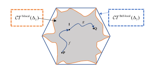
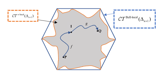
Corollary 2.1. (Path-connectedness)[31 , Appendix A] The set 𝒞 𝒯 bilocal ( Δ 3 ) 𝒞 superscript 𝒯 bilocal subscript Δ 3 \mathcal{CT}^{\textrm{bilocal}}(\Delta_{3}) is path-connected in the Hilbert space 𝒯 ( Δ 3 ) 𝒯 subscript Δ 3 \mathcal{T}(\Delta_{3}) 3
Figure 3: Path-connectness of the set 𝒞 𝒯 bilocal ( Δ 3 ) 𝒞 superscript 𝒯 bilocal subscript Δ 3 \mathcal{CT}^{\textrm{bilocal}}(\Delta_{3})
Proof. Let 𝐏 = P ( a b c | x y z ) 𝐏 𝑃 conditional 𝑎 𝑏 𝑐 𝑥 𝑦 𝑧 {\bf{P}}=\Lbrack P(abc|xyz)\Rbrack 𝐐 = Q ( a b c | x y z ) 𝐐 𝑄 conditional 𝑎 𝑏 𝑐 𝑥 𝑦 𝑧 {\bf{Q}}=\Lbrack Q(abc|xyz)\Rbrack 𝒞 𝒯 bilocal ( Δ 3 ) 𝒞 superscript 𝒯 bilocal subscript Δ 3 \mathcal{CT}^{\textrm{bilocal}}(\Delta_{3}) 𝐏 𝐏 {\bf{P}} 𝐐 𝐐 {\bf{Q}}
P ( a b c | x y z ) = ∑ λ 1 = 1 d 1 ∑ λ 2 = 1 d 2 p 1 ( λ 1 ) p 2 ( λ 2 ) P A ( a | x , λ 1 ) P B ( b | y , λ 1 λ 2 ) P C ( c | z , λ 2 ) 𝑃 conditional 𝑎 𝑏 𝑐 𝑥 𝑦 𝑧 superscript subscript subscript 𝜆 1 1 subscript 𝑑 1 superscript subscript subscript 𝜆 2 1 subscript 𝑑 2 subscript 𝑝 1 subscript 𝜆 1 subscript 𝑝 2 subscript 𝜆 2 subscript 𝑃 𝐴 conditional 𝑎 𝑥 subscript 𝜆 1
subscript 𝑃 𝐵 conditional 𝑏 𝑦 subscript 𝜆 1 subscript 𝜆 2
subscript 𝑃 𝐶 conditional 𝑐 𝑧 subscript 𝜆 2
P(abc|xyz)=\sum_{\lambda_{1}=1}^{d_{1}}\sum_{\lambda_{2}=1}^{d_{2}}p_{1}(\lambda_{1})p_{2}(\lambda_{2})P_{A}(a|x,\lambda_{1})P_{B}(b|y,\lambda_{1}\lambda_{2})P_{C}(c|z,\lambda_{2}) (2.20)
where
p i ( λ i ) , P A ( a | x , λ 1 ) , subscript 𝑝 𝑖 subscript 𝜆 𝑖 subscript 𝑃 𝐴 conditional 𝑎 𝑥 subscript 𝜆 1
p_{i}(\lambda_{i}),P_{A}(a|x,\lambda_{1}), P B ( b | y , λ 1 λ 2 ) , P C ( c | z , λ 2 ) subscript 𝑃 𝐵 conditional 𝑏 𝑦 subscript 𝜆 1 subscript 𝜆 2
subscript 𝑃 𝐶 conditional 𝑐 𝑧 subscript 𝜆 2
P_{B}(b|y,\lambda_{1}\lambda_{2}),P_{C}(c|z,\lambda_{2}) λ i , a , b , c , subscript 𝜆 𝑖 𝑎 𝑏 𝑐
\lambda_{i},a,b,c,
Q ( a b c | x y z ) = ∑ ξ 1 = 1 d 1 ′ ∑ ξ 2 = 1 d 2 ′ q 1 ( ξ 1 ) q 2 ( ξ 2 ) Q A ( a | x , ξ 1 ) Q B ( b | y , ξ 1 ξ 2 ) Q C ( c | z , ξ 2 ) 𝑄 conditional 𝑎 𝑏 𝑐 𝑥 𝑦 𝑧 superscript subscript subscript 𝜉 1 1 superscript subscript 𝑑 1 ′ superscript subscript subscript 𝜉 2 1 superscript subscript 𝑑 2 ′ subscript 𝑞 1 subscript 𝜉 1 subscript 𝑞 2 subscript 𝜉 2 subscript 𝑄 𝐴 conditional 𝑎 𝑥 subscript 𝜉 1
subscript 𝑄 𝐵 conditional 𝑏 𝑦 subscript 𝜉 1 subscript 𝜉 2
subscript 𝑄 𝐶 conditional 𝑐 𝑧 subscript 𝜉 2
Q(abc|xyz)=\sum_{\xi_{1}=1}^{d_{1}^{\prime}}\sum_{\xi_{2}=1}^{d_{2}^{\prime}}q_{1}(\xi_{1})q_{2}(\xi_{2})Q_{A}(a|x,\xi_{1})Q_{B}(b|y,\xi_{1}\xi_{2})Q_{C}(c|z,\xi_{2}) (2.21)
where q i ( ξ i ) , Q A ( a | x , ξ 1 ) , Q B ( b | y , ξ 1 ξ 2 ) , Q C ( c | z , ξ 2 ) subscript 𝑞 𝑖 subscript 𝜉 𝑖 subscript 𝑄 𝐴 conditional 𝑎 𝑥 subscript 𝜉 1
subscript 𝑄 𝐵 conditional 𝑏 𝑦 subscript 𝜉 1 subscript 𝜉 2
subscript 𝑄 𝐶 conditional 𝑐 𝑧 subscript 𝜉 2
q_{i}(\xi_{i}),Q_{A}(a|x,\xi_{1}),Q_{B}(b|y,\xi_{1}\xi_{2}),Q_{C}(c|z,\xi_{2}) ξ i , a , b , c , subscript 𝜉 𝑖 𝑎 𝑏 𝑐
\xi_{i},a,b,c,
Put I ( a b c | x y z ) ≡ 1 o A o B o C 𝐼 conditional 𝑎 𝑏 𝑐 𝑥 𝑦 𝑧 1 subscript 𝑜 𝐴 subscript 𝑜 𝐵 subscript 𝑜 𝐶 I(abc|xyz)\equiv\frac{1}{o_{A}o_{B}o_{C}} 𝐈 := I ( a b c | x y z ) ∈ 𝒞 𝒯 bilocal ( Δ 3 ) . assign 𝐈 𝐼 conditional 𝑎 𝑏 𝑐 𝑥 𝑦 𝑧 𝒞 superscript 𝒯 bilocal subscript Δ 3 {\bf{I}}:=\Lbrack I(abc|xyz)\Rbrack\in\mathcal{CT}^{\textrm{bilocal}}(\Delta_{3}). t ∈ [ 0 , 1 / 2 ] 𝑡 0 1 2 t\in[0,1/2]
P 1 t ( a | x , λ 1 ) = ( 1 − 2 t ) P 1 ( a | x , λ 1 ) + 2 t 1 o A ; subscript superscript 𝑃 𝑡 1 conditional 𝑎 𝑥 subscript 𝜆 1
1 2 𝑡 subscript 𝑃 1 conditional 𝑎 𝑥 subscript 𝜆 1
2 𝑡 1 subscript 𝑜 𝐴 P^{t}_{1}(a|x,\lambda_{1})=(1-2t)P_{1}(a|x,\lambda_{1})+2t\frac{1}{o_{A}};
P 2 t ( b | y , λ 1 λ 2 ) = ( 1 − 2 t ) P 2 ( b | y , λ 1 λ 2 ) + 2 t 1 o B ; subscript superscript 𝑃 𝑡 2 conditional 𝑏 𝑦 subscript 𝜆 1 subscript 𝜆 2
1 2 𝑡 subscript 𝑃 2 conditional 𝑏 𝑦 subscript 𝜆 1 subscript 𝜆 2
2 𝑡 1 subscript 𝑜 𝐵 P^{t}_{2}(b|y,\lambda_{1}\lambda_{2})=(1-2t)P_{2}(b|y,\lambda_{1}\lambda_{2})+2t\frac{1}{o_{B}};
P 3 t ( c | z , λ 2 ) = ( 1 − 2 t ) P 3 ( c | z , λ 2 ) + 2 t 1 o C , subscript superscript 𝑃 𝑡 3 conditional 𝑐 𝑧 subscript 𝜆 2
1 2 𝑡 subscript 𝑃 3 conditional 𝑐 𝑧 subscript 𝜆 2
2 𝑡 1 subscript 𝑜 𝐶 P^{t}_{3}(c|z,\lambda_{2})=(1-2t)P_{3}(c|z,\lambda_{2})+2t\frac{1}{o_{C}},
which are clearly PDs of a , b 𝑎 𝑏
a,b c 𝑐 c
P t ( a b c | x y z ) = ∑ λ 1 = 1 d 1 ∑ λ 2 = 1 d 2 p 1 ( λ 1 ) p 2 ( λ 2 ) P 1 t ( a | x , λ 1 ) P 2 t ( b | y , λ 1 λ 2 ) P 3 t ( c | z , λ 2 ) superscript 𝑃 𝑡 conditional 𝑎 𝑏 𝑐 𝑥 𝑦 𝑧 superscript subscript subscript 𝜆 1 1 subscript 𝑑 1 superscript subscript subscript 𝜆 2 1 subscript 𝑑 2 subscript 𝑝 1 subscript 𝜆 1 subscript 𝑝 2 subscript 𝜆 2 subscript superscript 𝑃 𝑡 1 conditional 𝑎 𝑥 subscript 𝜆 1
subscript superscript 𝑃 𝑡 2 conditional 𝑏 𝑦 subscript 𝜆 1 subscript 𝜆 2
subscript superscript 𝑃 𝑡 3 conditional 𝑐 𝑧 subscript 𝜆 2
\displaystyle P^{t}(abc|xyz)=\sum_{\lambda_{1}=1}^{d_{1}}\sum_{\lambda_{2}=1}^{d_{2}}p_{1}(\lambda_{1})p_{2}(\lambda_{2})P^{t}_{1}(a|x,\lambda_{1})P^{t}_{2}(b|y,\lambda_{1}\lambda_{2})P^{t}_{3}(c|z,\lambda_{2})
yields a bilocal CT
f ( t ) := P t ( a b c | x y z ) assign 𝑓 𝑡 superscript 𝑃 𝑡 conditional 𝑎 𝑏 𝑐 𝑥 𝑦 𝑧 {f}(t):=\Lbrack P^{t}(abc|xyz)\Rbrack Δ 3 subscript Δ 3 \Delta_{3} t ∈ [ 0 , 1 / 2 ] 𝑡 0 1 2 t\in[0,1/2] f ( 0 ) = 𝐏 𝑓 0 𝐏 {f}(0)={\bf{P}} f ( 1 / 2 ) = 𝐈 𝑓 1 2 𝐈 {f}(1/2)={\bf{I}} t ↦ f ( t ) maps-to 𝑡 𝑓 𝑡 t\mapsto{f}(t) [ 0 , 1 / 2 ] 0 1 2 [0,1/2] 𝒞 𝒯 bilocal ( Δ 3 ) 𝒞 superscript 𝒯 bilocal subscript Δ 3 \mathcal{CT}^{\textrm{bilocal}}(\Delta_{3})
Similarly, for every t ∈ [ 1 / 2 , 1 ] 𝑡 1 2 1 t\in[1/2,1]
Q 1 t ( a | x , ξ 1 ) = ( 2 t − 1 ) Q 1 ( a | x , ξ 1 ) + 2 ( 1 − t ) 1 o A ; subscript superscript 𝑄 𝑡 1 conditional 𝑎 𝑥 subscript 𝜉 1
2 𝑡 1 subscript 𝑄 1 conditional 𝑎 𝑥 subscript 𝜉 1
2 1 𝑡 1 subscript 𝑜 𝐴 Q^{t}_{1}(a|x,\xi_{1})=(2t-1)Q_{1}(a|x,\xi_{1})+2(1-t)\frac{1}{o_{A}};
Q 2 t ( b | y , ξ 1 ξ 2 ) = ( 2 t − 1 ) Q 2 ( b | y , ξ 1 ξ 2 ) + 2 ( 1 − t ) 1 o B ; subscript superscript 𝑄 𝑡 2 conditional 𝑏 𝑦 subscript 𝜉 1 subscript 𝜉 2
2 𝑡 1 subscript 𝑄 2 conditional 𝑏 𝑦 subscript 𝜉 1 subscript 𝜉 2
2 1 𝑡 1 subscript 𝑜 𝐵 Q^{t}_{2}(b|y,\xi_{1}\xi_{2})=(2t-1)Q_{2}(b|y,\xi_{1}\xi_{2})+2(1-t)\frac{1}{o_{B}};
Q 3 t ( c | z , ξ 2 ) = ( 2 t − 1 ) Q 3 ( c | z , ξ 2 ) + 2 ( 1 − t ) 1 o C , subscript superscript 𝑄 𝑡 3 conditional 𝑐 𝑧 subscript 𝜉 2
2 𝑡 1 subscript 𝑄 3 conditional 𝑐 𝑧 subscript 𝜉 2
2 1 𝑡 1 subscript 𝑜 𝐶 Q^{t}_{3}(c|z,\xi_{2})=(2t-1)Q_{3}(c|z,\xi_{2})+2(1-t)\frac{1}{o_{C}},
which are clearly PDs of a , b 𝑎 𝑏
a,b c 𝑐 c
Q t ( a b c | x y z ) = ∑ ξ 1 = 1 d 1 ′ ∑ ξ 2 = 1 d 2 ′ q 1 ( ξ 1 ) q 2 ( ξ 2 ) Q 1 t ( a | x , ξ 1 ) Q 2 t ( b | y , ξ 1 ξ 2 ) Q 3 t ( c | z , ξ 2 ) , superscript 𝑄 𝑡 conditional 𝑎 𝑏 𝑐 𝑥 𝑦 𝑧 superscript subscript subscript 𝜉 1 1 superscript subscript 𝑑 1 ′ superscript subscript subscript 𝜉 2 1 superscript subscript 𝑑 2 ′ subscript 𝑞 1 subscript 𝜉 1 subscript 𝑞 2 subscript 𝜉 2 subscript superscript 𝑄 𝑡 1 conditional 𝑎 𝑥 subscript 𝜉 1
subscript superscript 𝑄 𝑡 2 conditional 𝑏 𝑦 subscript 𝜉 1 subscript 𝜉 2
subscript superscript 𝑄 𝑡 3 conditional 𝑐 𝑧 subscript 𝜉 2
\displaystyle Q^{t}(abc|xyz)=\sum_{\xi_{1}=1}^{d_{1}^{\prime}}\sum_{\xi_{2}=1}^{d_{2}^{\prime}}q_{1}(\xi_{1})q_{2}(\xi_{2})Q^{t}_{1}(a|x,\xi_{1})Q^{t}_{2}(b|y,\xi_{1}\xi_{2})Q^{t}_{3}(c|z,\xi_{2}),
then
g ( t ) := Q t ( a b c | x y z ) assign 𝑔 𝑡 superscript 𝑄 𝑡 conditional 𝑎 𝑏 𝑐 𝑥 𝑦 𝑧 {g}(t):=\Lbrack Q^{t}(abc|xyz)\Rbrack Δ 3 subscript Δ 3 \Delta_{3} t ∈ [ 1 / 2 , 1 ] 𝑡 1 2 1 t\in[1/2,1] g ( 1 / 2 ) = 𝐈 𝑔 1 2 𝐈 {g}(1/2)={\bf{I}} g ( 1 ) = 𝐐 𝑔 1 𝐐 {g}(1)={\bf{Q}} t ↦ g ( t ) maps-to 𝑡 𝑔 𝑡 t\mapsto{g}(t) [ 1 / 2 , 1 ] 1 2 1 [1/2,1] 𝒞 𝒯 bilocal ( Δ 3 ) 𝒞 superscript 𝒯 bilocal subscript Δ 3 \mathcal{CT}^{\textrm{bilocal}}(\Delta_{3}) f : [ 0 , 1 ] → 𝒞 𝒯 bilocal ( Δ 3 ) : 𝑓 → 0 1 𝒞 superscript 𝒯 bilocal subscript Δ 3 f:[0,1]\rightarrow\mathcal{CT}^{\textrm{bilocal}}(\Delta_{3})
p ( t ) = { f ( t ) , t ∈ [ 0 , 1 / 2 ] ; g ( t ) , t ∈ ( 1 / 2 , 1 ] , 𝑝 𝑡 cases 𝑓 𝑡 𝑡 0 1 2 𝑔 𝑡 𝑡 1 2 1 p(t)=\left\{\begin{array}[]{cc}{f}(t),&t\in[0,1/2];\\
{g}(t),&t\in(1/2,1],\end{array}\right.
is continuous everywhere
and then induces a path p 𝑝 p 𝒞 𝒯 bilocal ( Δ 3 ) 𝒞 superscript 𝒯 bilocal subscript Δ 3 \mathcal{CT}^{\textrm{bilocal}}(\Delta_{3}) 𝐏 𝐏 {\bf{P}} 𝐐 𝐐 {\bf{Q}} 𝒞 𝒯 bilocal ( Δ 3 ) 𝒞 superscript 𝒯 bilocal subscript Δ 3 \mathcal{CT}^{\textrm{bilocal}}(\Delta_{3})
Next, let us discuss the star-convexity of the set of all bilocal CTs over Δ 3 subscript Δ 3 \Delta_{3} D 𝐷 D V 𝑉 V s 𝑠 s S 𝑆 S ( 1 − t ) s + t D ⊂ D 1 𝑡 𝑠 𝑡 𝐷 𝐷 (1-t)s+tD\subset D t ∈ [ 0 , 1 ] . 𝑡 0 1 t\in[0,1].
To do this, take a CT 𝐄 = E ( a | x ) 𝐄 𝐸 conditional 𝑎 𝑥 {\bf{E}}=\Lbrack E(a|x)\Rbrack [ o A ] × [ m A ] delimited-[] subscript 𝑜 𝐴 delimited-[] subscript 𝑚 𝐴 [o_{A}]\times[m_{A}]
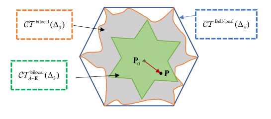
𝒞 𝒯 A − 𝐄 bilocal ( Δ 3 ) = { 𝐏 ∈ 𝒞 𝒯 bilocal ( Δ 3 ) : 𝐏 A = 𝐄 } . 𝒞 superscript subscript 𝒯 𝐴 𝐄 bilocal subscript Δ 3 conditional-set 𝐏 𝒞 superscript 𝒯 bilocal subscript Δ 3 subscript 𝐏 𝐴 𝐄 \mathcal{CT}_{A-{\bf{E}}}^{\textrm{bilocal}}(\Delta_{3})=\left\{{\bf{P}}\in\mathcal{CT}^{\textrm{bilocal}}(\Delta_{3}):\ {\bf{P}}_{A}={\bf{E}}\right\}.
The proof of the following corollary is suggested by an argument in [31 , Appendix A.2] .
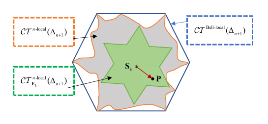
Corollary 2.2. (Star-convexity)[31 , Appendix A.2] The set 𝒞 𝒯 A − 𝐄 bilocal ( Δ 3 ) 𝒞 superscript subscript 𝒯 𝐴 𝐄 bilocal subscript Δ 3 \mathcal{CT}_{A-{\bf{E}}}^{\textrm{bilocal}}(\Delta_{3}) is star-convex the Hilbert space 𝒯 ( Δ 3 ) 𝒯 subscript Δ 3 \mathcal{T}(\Delta_{3}) 4
Figure 4: Star-convexity of the set 𝒞 𝒯 A − 𝐄 bilocal ( Δ 3 ) 𝒞 superscript subscript 𝒯 𝐴 𝐄 bilocal subscript Δ 3 \mathcal{CT}_{A-{\bf{E}}}^{\textrm{bilocal}}(\Delta_{3})
Proof. Put P 0 ( a b c | x y z ) = E ( a | x ) × 1 o B × 1 o C subscript 𝑃 0 conditional 𝑎 𝑏 𝑐 𝑥 𝑦 𝑧 𝐸 conditional 𝑎 𝑥 1 subscript 𝑜 𝐵 1 subscript 𝑜 𝐶 P_{0}(abc|xyz)=E(a|x)\times\frac{1}{o_{B}}\times\frac{1}{o_{C}} 𝐏 0 := P 0 ( a b c | x y z ) assign subscript 𝐏 0 subscript 𝑃 0 conditional 𝑎 𝑏 𝑐 𝑥 𝑦 𝑧 {\bf{P}}_{0}:=\Lbrack P_{0}(abc|xyz)\Rbrack Δ 3 subscript Δ 3 \Delta_{3} 𝐏 0 subscript 𝐏 0 {\bf{P}}_{0} 𝒞 𝒯 A − 𝐄 bilocal ( Δ 3 ) 𝒞 superscript subscript 𝒯 𝐴 𝐄 bilocal subscript Δ 3 \mathcal{CT}_{A-{\bf{E}}}^{\textrm{bilocal}}(\Delta_{3})
( 1 − t ) 𝐏 0 + t 𝒞 𝒯 A − 𝐄 bilocal ( Δ 3 ) ⊂ 𝒞 𝒯 A − 𝐄 bilocal ( Δ 3 ) , ∀ t ∈ [ 0 , 1 ] . formulae-sequence 1 𝑡 subscript 𝐏 0 𝑡 𝒞 superscript subscript 𝒯 𝐴 𝐄 bilocal subscript Δ 3 𝒞 superscript subscript 𝒯 𝐴 𝐄 bilocal subscript Δ 3 for-all 𝑡 0 1 (1-t){\bf{P}}_{0}+t\mathcal{CT}_{A-{\bf{E}}}^{\textrm{bilocal}}(\Delta_{3})\subset\mathcal{CT}_{A-{\bf{E}}}^{\textrm{bilocal}}(\Delta_{3}),\ \forall t\in[0,1]. (2.22)
Let
𝐏 = P ( a b c | x y z ) ∈ 𝒞 𝒯 A − 𝐄 bilocal ( Δ 3 ) 𝐏 𝑃 conditional 𝑎 𝑏 𝑐 𝑥 𝑦 𝑧 𝒞 superscript subscript 𝒯 𝐴 𝐄 bilocal subscript Δ 3 {\bf{P}}=\Lbrack P(abc|xyz)\Rbrack\in\mathcal{CT}_{A-{\bf{E}}}^{\textrm{bilocal}}(\Delta_{3}) 𝐏 𝐏 {\bf{P}}
P ( a b c | x y z ) = ∑ λ 1 = 1 d 1 ∑ λ 2 = 1 d 2 p 1 ( λ 1 ) p 2 ( λ 2 ) P A ( a | x , λ 1 ) P B ( b | y , λ 1 λ 2 ) P C ( c | z , λ 2 ) . 𝑃 conditional 𝑎 𝑏 𝑐 𝑥 𝑦 𝑧 superscript subscript subscript 𝜆 1 1 subscript 𝑑 1 superscript subscript subscript 𝜆 2 1 subscript 𝑑 2 subscript 𝑝 1 subscript 𝜆 1 subscript 𝑝 2 subscript 𝜆 2 subscript 𝑃 𝐴 conditional 𝑎 𝑥 subscript 𝜆 1
subscript 𝑃 𝐵 conditional 𝑏 𝑦 subscript 𝜆 1 subscript 𝜆 2
subscript 𝑃 𝐶 conditional 𝑐 𝑧 subscript 𝜆 2
P(abc|xyz)=\sum_{\lambda_{1}=1}^{d_{1}}\sum_{\lambda_{2}=1}^{d_{2}}p_{1}(\lambda_{1})p_{2}(\lambda_{2})P_{A}(a|x,\lambda_{1})P_{B}(b|y,\lambda_{1}\lambda_{2})P_{C}(c|z,\lambda_{2}). (2.23)
The condition P A ( a | x ) = E ( a | x ) subscript 𝑃 𝐴 conditional 𝑎 𝑥 𝐸 conditional 𝑎 𝑥 P_{A}(a|x)=E(a|x)
∑ λ 1 = 1 d 1 p 1 ( λ 1 ) P A ( a | x , λ 1 ) = E ( a | x ) , ∀ x ∈ [ m A ] , a ∈ [ o A ] . formulae-sequence superscript subscript subscript 𝜆 1 1 subscript 𝑑 1 subscript 𝑝 1 subscript 𝜆 1 subscript 𝑃 𝐴 conditional 𝑎 𝑥 subscript 𝜆 1
𝐸 conditional 𝑎 𝑥 formulae-sequence for-all 𝑥 delimited-[] subscript 𝑚 𝐴 𝑎 delimited-[] subscript 𝑜 𝐴 \sum_{\lambda_{1}=1}^{d_{1}}p_{1}(\lambda_{1})P_{A}(a|x,\lambda_{1})=E(a|x),\ \forall x\in[m_{A}],a\in[o_{A}]. (2.24)
For every t ∈ [ 0 , 1 ] 𝑡 0 1 t\in[0,1]
f ( λ 2 , s ) = { p 2 ( λ 2 ) ( 1 − t ) , s = 0 ; p 2 ( λ 2 ) t , s = 1 , 𝑓 subscript 𝜆 2 𝑠 cases subscript 𝑝 2 subscript 𝜆 2 1 𝑡 𝑠 0 subscript 𝑝 2 subscript 𝜆 2 𝑡 𝑠 1 f(\lambda_{2},s)=\left\{\begin{array}[]{cc}p_{2}(\lambda_{2})(1-t),&s=0;\\
p_{2}(\lambda_{2})t,&s=1,\end{array}\right.
P B ( b | y , λ 1 , ( λ 2 , s ) ) = { 1 o B , s = 0 ; P B ( b | y , λ 1 λ 2 ) , s = 1 , subscript 𝑃 𝐵 conditional 𝑏 𝑦 subscript 𝜆 1 subscript 𝜆 2 𝑠
cases 1 subscript 𝑜 𝐵 𝑠 0 subscript 𝑃 𝐵 conditional 𝑏 𝑦 subscript 𝜆 1 subscript 𝜆 2
𝑠 1 P_{B}(b|y,\lambda_{1},(\lambda_{2},s))=\left\{\begin{array}[]{cc}\frac{1}{o_{B}},&s=0;\\
P_{B}(b|y,\lambda_{1}\lambda_{2}),&s=1,\end{array}\right.
P C ( c | z , ( λ 2 , s ) ) = { 1 o C , s = 0 ; P C ( c | z , λ 2 ) , s = 1 , subscript 𝑃 𝐶 conditional 𝑐 𝑧 subscript 𝜆 2 𝑠
cases 1 subscript 𝑜 𝐶 𝑠 0 subscript 𝑃 𝐶 conditional 𝑐 𝑧 subscript 𝜆 2
𝑠 1 P_{C}(c|z,(\lambda_{2},s))=\left\{\begin{array}[]{cc}\frac{1}{o_{C}},&s=0;\\
P_{C}(c|z,\lambda_{2}),&s=1,\end{array}\right.
which are PDs of ( λ 2 , s ) , b subscript 𝜆 2 𝑠 𝑏
(\lambda_{2},s),b c 𝑐 c x , y , z , a , b , z 𝑥 𝑦 𝑧 𝑎 𝑏 𝑧
x,y,z,a,b,z 2.24
∑ λ 1 ∈ [ d 1 ] ∑ ( λ 2 , s ) ∈ [ d 2 ] × { 0 , 1 } p 1 ( λ 1 ) f ( λ 2 , s ) P A ( a | x , λ 1 ) subscript subscript 𝜆 1 delimited-[] subscript 𝑑 1 subscript subscript 𝜆 2 𝑠 delimited-[] subscript 𝑑 2 0 1 subscript 𝑝 1 subscript 𝜆 1 𝑓 subscript 𝜆 2 𝑠 subscript 𝑃 𝐴 conditional 𝑎 𝑥 subscript 𝜆 1
\displaystyle\sum_{\lambda_{1}\in[d_{1}]}\sum_{(\lambda_{2},s)\in[d_{2}]\times\{0,1\}}p_{1}(\lambda_{1})f(\lambda_{2},s)P_{A}(a|x,\lambda_{1})
× P B ( b | y , λ 1 ( λ 2 , s ) ) P C ( c | z , λ 2 ( λ 2 , s ) ) absent subscript 𝑃 𝐵 conditional 𝑏 𝑦 subscript 𝜆 1 subscript 𝜆 2 𝑠
subscript 𝑃 𝐶 conditional 𝑐 𝑧 subscript 𝜆 2 subscript 𝜆 2 𝑠
\displaystyle\times P_{B}(b|y,\lambda_{1}(\lambda_{2},s))P_{C}(c|z,\lambda_{2}(\lambda_{2},s))
= \displaystyle= ∑ λ 1 ∈ [ d 1 ] ∑ λ 2 ∈ [ d 2 ] p 1 ( λ 1 ) p 2 ( λ 2 ) ( 1 − t ) P A ( a | x , λ 1 ) 1 o B 1 o C subscript subscript 𝜆 1 delimited-[] subscript 𝑑 1 subscript subscript 𝜆 2 delimited-[] subscript 𝑑 2 subscript 𝑝 1 subscript 𝜆 1 subscript 𝑝 2 subscript 𝜆 2 1 𝑡 subscript 𝑃 𝐴 conditional 𝑎 𝑥 subscript 𝜆 1
1 subscript 𝑜 𝐵 1 subscript 𝑜 𝐶 \displaystyle\sum_{\lambda_{1}\in[d_{1}]}\sum_{\lambda_{2}\in[d_{2}]}p_{1}(\lambda_{1})p_{2}(\lambda_{2})(1-t)P_{A}(a|x,\lambda_{1})\frac{1}{o_{B}}\frac{1}{o_{C}}
+ ∑ λ 1 ∈ [ d 1 ] ∑ λ 2 ∈ [ d 2 ] p 1 ( λ 1 ) p 2 ( λ 2 ) t P A ( a | x , λ 1 ) P B ( b | y , λ 1 λ 2 ) P C ( c | z , λ 2 ) subscript subscript 𝜆 1 delimited-[] subscript 𝑑 1 subscript subscript 𝜆 2 delimited-[] subscript 𝑑 2 subscript 𝑝 1 subscript 𝜆 1 subscript 𝑝 2 subscript 𝜆 2 𝑡 subscript 𝑃 𝐴 conditional 𝑎 𝑥 subscript 𝜆 1
subscript 𝑃 𝐵 conditional 𝑏 𝑦 subscript 𝜆 1 subscript 𝜆 2
subscript 𝑃 𝐶 conditional 𝑐 𝑧 subscript 𝜆 2
\displaystyle+\sum_{\lambda_{1}\in[d_{1}]}\sum_{\lambda_{2}\in[d_{2}]}p_{1}(\lambda_{1})p_{2}(\lambda_{2})tP_{A}(a|x,\lambda_{1})P_{B}(b|y,\lambda_{1}\lambda_{2})P_{C}(c|z,\lambda_{2})
= \displaystyle= ( 1 − t ) P 0 ( a b c | x y z ) + t P ( a b c | x y z ) . 1 𝑡 subscript 𝑃 0 conditional 𝑎 𝑏 𝑐 𝑥 𝑦 𝑧 𝑡 𝑃 conditional 𝑎 𝑏 𝑐 𝑥 𝑦 𝑧 \displaystyle(1-t)P_{0}(abc|xyz)+tP(abc|xyz).
This shows that 𝐐 := ( 1 − t ) 𝐏 0 + t 𝐏 assign 𝐐 1 𝑡 subscript 𝐏 0 𝑡 𝐏 {\bf{Q}}:=(1-t){\bf{P}}_{0}+t{\bf{P}} 𝐐 A = 𝐄 subscript 𝐐 𝐴 𝐄 {\bf{Q}}_{A}={\bf{E}} 𝐏 ∈ 𝒞 𝒯 A − 𝐄 bilocal ( Δ 3 ) 𝐏 𝒞 superscript subscript 𝒯 𝐴 𝐄 bilocal subscript Δ 3 {\bf{P}}\in\mathcal{CT}_{A-{\bf{E}}}^{\textrm{bilocal}}(\Delta_{3}) 2.22 𝒞 𝒯 A − 𝐄 bilocal ( Δ 3 ) 𝒞 superscript subscript 𝒯 𝐴 𝐄 bilocal subscript Δ 3 \mathcal{CT}_{A-{\bf{E}}}^{\textrm{bilocal}}(\Delta_{3}) 𝐏 0 subscript 𝐏 0 {\bf{P}}_{0}
Similarly, for any fixed CT 𝐅 = F ( c | z ) 𝐅 𝐹 conditional 𝑐 𝑧 {\bf{F}}=\Lbrack F(c|z)\Rbrack [ o C ] × [ m C ] delimited-[] subscript 𝑜 𝐶 delimited-[] subscript 𝑚 𝐶 [o_{C}]\times[m_{C}]
𝒞 𝒯 C − 𝐅 bilocal ( Δ 3 ) = { 𝐏 ∈ 𝒞 𝒯 bilocal ( Δ 3 ) : 𝐏 C = 𝐅 } 𝒞 superscript subscript 𝒯 𝐶 𝐅 bilocal subscript Δ 3 conditional-set 𝐏 𝒞 superscript 𝒯 bilocal subscript Δ 3 subscript 𝐏 𝐶 𝐅 \mathcal{CT}_{C-{\bf{F}}}^{\textrm{bilocal}}(\Delta_{3})=\left\{{\bf{P}}\in\mathcal{CT}^{\textrm{bilocal}}(\Delta_{3}):\ {\bf{P}}_{C}={\bf{F}}\right\}
is also star-convex.
Another application of Theorem 2.1 is to prove the compactness of 𝒞 𝒯 bilocal ( Δ 3 ) 𝒞 superscript 𝒯 bilocal subscript Δ 3 \mathcal{CT}^{\textrm{bilocal}}(\Delta_{3})
Corollary 2.3. (Compactness) The set 𝒞 𝒯 bilocal ( Δ 3 ) 𝒞 superscript 𝒯 bilocal subscript Δ 3 \mathcal{CT}^{\textrm{bilocal}}(\Delta_{3}) is compact in the Hilbert space 𝒯 ( Δ 3 ) 𝒯 subscript Δ 3 \mathcal{T}(\Delta_{3})
Proof. Let P ∈ 𝒞 𝒯 ( Δ 3 ) P 𝒞 𝒯 subscript Δ 3 \textbf{P}\in\mathcal{CT}(\Delta_{3}) { 𝐏 n } n = 1 ∞ ⊂ 𝒞 𝒯 bilocal ( Δ 3 ) superscript subscript subscript 𝐏 𝑛 𝑛 1 𝒞 superscript 𝒯 bilocal subscript Δ 3 \{{\bf{P}}_{n}\}_{n=1}^{\infty}\subset\mathcal{CT}^{\textrm{bilocal}}(\Delta_{3}) P n → P → subscript P 𝑛 P \textbf{P}_{n}\rightarrow\textbf{P} n → ∞ → 𝑛 n\rightarrow\infty P n ( a b c | x y z ) → P ( a b c | x y z ) → subscript 𝑃 𝑛 conditional 𝑎 𝑏 𝑐 𝑥 𝑦 𝑧 𝑃 conditional 𝑎 𝑏 𝑐 𝑥 𝑦 𝑧 P_{n}(abc|xyz)\rightarrow P(abc|xyz) n → ∞ → 𝑛 n\rightarrow\infty ( a , b , c , x , y , z ) ∈ Δ 3 𝑎 𝑏 𝑐 𝑥 𝑦 𝑧 subscript Δ 3 (a,b,c,x,y,z)\in\Delta_{3}
P n ( a b c | x y z ) = ∑ i = 1 N A ∑ k = 1 N C π 1 ( n ) ( i ) π 2 ( n ) ( k ) δ a , J i ( x ) P B ( n ) ( b | y , i , k ) δ c , L k ( z ) subscript 𝑃 𝑛 conditional 𝑎 𝑏 𝑐 𝑥 𝑦 𝑧 superscript subscript 𝑖 1 subscript 𝑁 𝐴 superscript subscript 𝑘 1 subscript 𝑁 𝐶 subscript superscript 𝜋 𝑛 1 𝑖 subscript superscript 𝜋 𝑛 2 𝑘 subscript 𝛿 𝑎 subscript 𝐽 𝑖 𝑥
subscript superscript 𝑃 𝑛 𝐵 conditional 𝑏 𝑦 𝑖 𝑘
subscript 𝛿 𝑐 subscript 𝐿 𝑘 𝑧
P_{n}(abc|xyz)=\sum_{i=1}^{N_{A}}\sum_{k=1}^{N_{C}}\pi^{(n)}_{1}(i)\pi^{(n)}_{2}(k)\delta_{a,J_{i}(x)}P^{(n)}_{B}(b|y,i,k)\delta_{c,L_{k}(z)} (2.25)
for all x , a , y , b , z , c , 𝑥 𝑎 𝑦 𝑏 𝑧 𝑐
x,a,y,b,z,c, n = 1 , 2 , … , 𝑛 1 2 …
n=1,2,\ldots,
{ π 1 ( n ) ( i ) } i ∈ [ N A ] , { π 2 ( n ) ( k ) } k ∈ [ N C ] , and { P B ( n ) ( b | y , i , k ) } b ∈ [ o B ] ( ∀ y , i , k ) subscript subscript superscript 𝜋 𝑛 1 𝑖 𝑖 delimited-[] subscript 𝑁 𝐴 subscript subscript superscript 𝜋 𝑛 2 𝑘 𝑘 delimited-[] subscript 𝑁 𝐶 and subscript subscript superscript 𝑃 𝑛 𝐵 conditional 𝑏 𝑦 𝑖 𝑘
𝑏 delimited-[] subscript 𝑜 𝐵 for-all 𝑦 𝑖 𝑘
\{\pi^{(n)}_{1}(i)\}_{i\in[N_{A}]},\ \{\pi^{(n)}_{2}(k)\}_{k\in[N_{C}]},{\rm{\ and\ }}\{P^{(n)}_{B}(b|y,i,k)\}_{b\in[o_{B}]}(\forall y,i,k)
are PDs of i , k , b 𝑖 𝑘 𝑏
i,k,b
lim n → ∞ π 1 ( n ) ( i ) = π 1 ( i ) ( ∀ i ) , lim n → ∞ π 2 ( n ) ( k ) = π 2 ( k ) ( ∀ k ) , formulae-sequence subscript → 𝑛 subscript superscript 𝜋 𝑛 1 𝑖 subscript 𝜋 1 𝑖 for-all 𝑖 subscript → 𝑛 subscript superscript 𝜋 𝑛 2 𝑘 subscript 𝜋 2 𝑘 for-all 𝑘 \lim_{n\rightarrow\infty}\pi^{(n)}_{1}(i)=\pi_{1}(i)(\forall i),\ \lim_{n\rightarrow\infty}\pi^{(n)}_{2}(k)=\pi_{2}(k)(\forall k),
and
lim n → ∞ P B ( n ) ( b | y , i , k ) = P B ( b | y , i , k ) ( ∀ y , b , i , k ) . subscript → 𝑛 subscript superscript 𝑃 𝑛 𝐵 conditional 𝑏 𝑦 𝑖 𝑘
subscript 𝑃 𝐵 conditional 𝑏 𝑦 𝑖 𝑘
for-all 𝑦 𝑏 𝑖 𝑘 \lim_{n\rightarrow\infty}P^{(n)}_{B}(b|y,i,k)=P_{B}(b|y,i,k)(\forall y,b,i,k).
Obviously, { π 1 ( i ) } i ∈ [ N A ] subscript subscript 𝜋 1 𝑖 𝑖 delimited-[] subscript 𝑁 𝐴 \{\pi_{1}(i)\}_{i\in[N_{A}]} { π 2 ( k ) } k ∈ [ N C ] subscript subscript 𝜋 2 𝑘 𝑘 delimited-[] subscript 𝑁 𝐶 \{\pi_{2}(k)\}_{k\in[N_{C}]} { P B ( b | y , i , k ) } b ∈ [ o B ] ( ∀ y , i , k ) subscript subscript 𝑃 𝐵 conditional 𝑏 𝑦 𝑖 𝑘
𝑏 delimited-[] subscript 𝑜 𝐵 for-all 𝑦 𝑖 𝑘 \{P_{B}(b|y,i,k)\}_{b\in[o_{B}]}(\forall y,i,k) i , k , b 𝑖 𝑘 𝑏
i,k,b n → ∞ → 𝑛 n\rightarrow\infty 2.25
P ( a b c | x y z ) = ∑ i = 1 N A ∑ k = 1 N C π 1 ( i ) π 2 ( k ) δ a , J i ( x ) P B ( b | y , i , k ) δ c , L k ( z ) , ∀ x , a , y , b , z , c . 𝑃 conditional 𝑎 𝑏 𝑐 𝑥 𝑦 𝑧 superscript subscript 𝑖 1 subscript 𝑁 𝐴 superscript subscript 𝑘 1 subscript 𝑁 𝐶 subscript 𝜋 1 𝑖 subscript 𝜋 2 𝑘 subscript 𝛿 𝑎 subscript 𝐽 𝑖 𝑥
subscript 𝑃 𝐵 conditional 𝑏 𝑦 𝑖 𝑘
subscript 𝛿 𝑐 subscript 𝐿 𝑘 𝑧
for-all 𝑥 𝑎 𝑦 𝑏 𝑧 𝑐
P(abc|xyz)=\sum_{i=1}^{N_{A}}\sum_{k=1}^{N_{C}}\pi_{1}(i)\pi_{2}(k)\delta_{a,J_{i}(x)}P_{B}(b|y,i,k)\delta_{c,L_{k}(z)},\ \forall x,a,y,b,z,c.
Using Theorem 2.1 again implies that
𝐏 ∈ 𝒞 𝒯 bilocal ( Δ 3 ) 𝐏 𝒞 superscript 𝒯 bilocal subscript Δ 3 {\bf{P}}\in\mathcal{CT}^{\textrm{bilocal}}(\Delta_{3}) 𝒞 𝒯 bilocal ( Δ 3 ) 𝒞 superscript 𝒯 bilocal subscript Δ 3 \mathcal{CT}^{\textrm{bilocal}}(\Delta_{3})
Similar to Definition 2.1 we can introduce and discuss bilocality of a tripartite CT 𝐏 = P ( a b c | x y z ) 𝐏 𝑃 conditional 𝑎 𝑏 𝑐 𝑥 𝑦 𝑧 {\bf{P}}=\Lbrack P(abc|xyz)\Rbrack Δ 3 subscript Δ 3 \Delta_{3}
P ( a b c | x y z ) 𝑃 conditional 𝑎 𝑏 𝑐 𝑥 𝑦 𝑧 \displaystyle P(abc|xyz) = \displaystyle= ∬ Λ 1 × Λ 2 q 1 ( λ 1 ) q 2 ( λ 2 ) P A ( a | x , λ 1 λ 2 ) subscript double-integral subscript Λ 1 subscript Λ 2 subscript 𝑞 1 subscript 𝜆 1 subscript 𝑞 2 subscript 𝜆 2 subscript 𝑃 𝐴 conditional 𝑎 𝑥 subscript 𝜆 1 subscript 𝜆 2
\displaystyle\iint_{\Lambda_{1}\times\Lambda_{2}}q_{1}(\lambda_{1})q_{2}(\lambda_{2})P_{A}(a|x,\lambda_{1}\lambda_{2}) (2.26)
× P B ( b | y , λ 1 ) P C ( c | z , λ 2 ) d μ 1 ( λ 1 ) d μ 2 ( λ 2 ) absent subscript 𝑃 𝐵 conditional 𝑏 𝑦 subscript 𝜆 1
subscript 𝑃 𝐶 conditional 𝑐 𝑧 subscript 𝜆 2
d subscript 𝜇 1 subscript 𝜆 1 d subscript 𝜇 2 subscript 𝜆 2 \displaystyle\times P_{B}(b|y,\lambda_{1})P_{C}(c|z,\lambda_{2}){\rm{d}}\mu_{1}(\lambda_{1}){\rm{d}}\mu_{2}(\lambda_{2})
or
P ( a b c | x y z ) 𝑃 conditional 𝑎 𝑏 𝑐 𝑥 𝑦 𝑧 \displaystyle P(abc|xyz) = \displaystyle= ∬ Λ 1 × Λ 2 q 1 ( λ 1 ) q 2 ( λ 2 ) P A ( a | x , λ 1 ) subscript double-integral subscript Λ 1 subscript Λ 2 subscript 𝑞 1 subscript 𝜆 1 subscript 𝑞 2 subscript 𝜆 2 subscript 𝑃 𝐴 conditional 𝑎 𝑥 subscript 𝜆 1
\displaystyle\iint_{\Lambda_{1}\times\Lambda_{2}}q_{1}(\lambda_{1})q_{2}(\lambda_{2})P_{A}(a|x,\lambda_{1}) (2.27)
× P B ( b | y , λ 2 ) P C ( c | z , λ 1 λ 2 ) d μ 1 ( λ 1 ) d μ 2 ( λ 2 ) . absent subscript 𝑃 𝐵 conditional 𝑏 𝑦 subscript 𝜆 2
subscript 𝑃 𝐶 conditional 𝑐 𝑧 subscript 𝜆 1 subscript 𝜆 2
d subscript 𝜇 1 subscript 𝜆 1 d subscript 𝜇 2 subscript 𝜆 2 \displaystyle\times P_{B}(b|y,\lambda_{2})P_{C}(c|z,\lambda_{1}\lambda_{2}){\rm{d}}\mu_{1}(\lambda_{1}){\rm{d}}\mu_{2}(\lambda_{2}).
The last type here of bilocality is just the special case of n 𝑛 n n = 2 𝑛 2 n=2 2 2 2
3 Bilocality of probability tensors
The usual Bell nonlocality of a quantum state or a quantum network is the property that is exhibited by performing a set of non-compatible local POVM measurements. Renou et al. [43 ] pointed out that
quantum nonlocality in a quantum network can be demonstrated without the need of having various input settings, but only by considering the joint statistics of fixed local measurement outputs. For example, for a tripartite network, it suffices to consider the tripartite probability distribution { P ( a , b , c ) } 𝑃 𝑎 𝑏 𝑐 \{P(a,b,c)\} a , b , c 𝑎 𝑏 𝑐
a,b,c a ∈ [ o A ] , b ∈ [ o B ] formulae-sequence 𝑎 delimited-[] subscript 𝑜 𝐴 𝑏 delimited-[] subscript 𝑜 𝐵 a\in[o_{A}],b\in[o_{B}] c ∈ [ o C ] 𝑐 delimited-[] subscript 𝑜 𝐶 c\in[o_{C}] 𝐏 = P ( a , b , c ) 𝐏 𝑃 𝑎 𝑏 𝑐 {\bf{P}}=\Lbrack P(a,b,c)\Rbrack O 3 = [ o A ] × [ o B ] × [ o C ] subscript 𝑂 3 delimited-[] subscript 𝑜 𝐴 delimited-[] subscript 𝑜 𝐵 delimited-[] subscript 𝑜 𝐶 O_{3}=[o_{A}]\times[o_{B}]\times[o_{C}] probability tensor (PT)[45 ] . Note that every PT 𝐏 = P ( a , b , c ) 𝐏 𝑃 𝑎 𝑏 𝑐 {\bf{P}}=\Lbrack P(a,b,c)\Rbrack O 3 subscript 𝑂 3 O_{3}
P ( a , b , c ) = ∑ λ = ( λ 1 , λ 2 , λ 3 ) ∈ O 3 q ( λ ) P A ( a | λ ) P B ( b | λ ) P C ( c | λ ) ( ∀ a , b , c ) , 𝑃 𝑎 𝑏 𝑐 subscript 𝜆 subscript 𝜆 1 subscript 𝜆 2 subscript 𝜆 3 subscript 𝑂 3 𝑞 𝜆 subscript 𝑃 𝐴 conditional 𝑎 𝜆 subscript 𝑃 𝐵 conditional 𝑏 𝜆 subscript 𝑃 𝐶 conditional 𝑐 𝜆 for-all 𝑎 𝑏 𝑐 P(a,b,c)=\sum_{\lambda=(\lambda_{1},\lambda_{2},\lambda_{3})\in O_{3}}q(\lambda)P_{A}(a|\lambda)P_{B}(b|\lambda)P_{C}(c|\lambda)(\forall a,b,c),
where
q ( λ ) = P ( λ 1 , λ 2 , λ 3 ) , P A ( a | λ ) = δ a , λ 1 , P B ( b | λ ) = δ b , λ 2 , P C ( c | λ ) = δ c , λ 3 , formulae-sequence 𝑞 𝜆 𝑃 subscript 𝜆 1 subscript 𝜆 2 subscript 𝜆 3 formulae-sequence subscript 𝑃 𝐴 conditional 𝑎 𝜆 subscript 𝛿 𝑎 subscript 𝜆 1
formulae-sequence subscript 𝑃 𝐵 conditional 𝑏 𝜆 subscript 𝛿 𝑏 subscript 𝜆 2
subscript 𝑃 𝐶 conditional 𝑐 𝜆 subscript 𝛿 𝑐 subscript 𝜆 3
q(\lambda)=P(\lambda_{1},\lambda_{2},\lambda_{3}),P_{A}(a|\lambda)=\delta_{a,\lambda_{1}},P_{B}(b|\lambda)=\delta_{b,\lambda_{2}},P_{C}(c|\lambda)=\delta_{c,\lambda_{3}},
which a PDs of λ , a , b 𝜆 𝑎 𝑏
\lambda,a,b c 𝑐 c 𝐏 𝐏 {\bf{P}}
Definition 3.1. A PT 𝐏 = P ( a , b , c ) 𝐏 𝑃 𝑎 𝑏 𝑐 {\bf{P}}=\Lbrack P(a,b,c)\Rbrack O 3 subscript 𝑂 3 O_{3} bilocal if it admits a C-biLHVM:
P ( a , b , c ) = ∬ Λ 1 × Λ 2 q 1 ( λ 1 ) q 2 ( λ 2 ) P A ( a | λ 1 ) P B ( b | λ 1 λ 2 ) P C ( c | λ 2 ) d μ 1 ( λ 1 ) d μ 2 ( λ 2 ) 𝑃 𝑎 𝑏 𝑐 subscript double-integral subscript Λ 1 subscript Λ 2 subscript 𝑞 1 subscript 𝜆 1 subscript 𝑞 2 subscript 𝜆 2 subscript 𝑃 𝐴 conditional 𝑎 subscript 𝜆 1 subscript 𝑃 𝐵 conditional 𝑏 subscript 𝜆 1 subscript 𝜆 2 subscript 𝑃 𝐶 conditional 𝑐 subscript 𝜆 2 differential-d subscript 𝜇 1 subscript 𝜆 1 differential-d subscript 𝜇 2 subscript 𝜆 2 P(a,b,c)=\iint_{\Lambda_{1}\times\Lambda_{2}}q_{1}(\lambda_{1})q_{2}(\lambda_{2})P_{A}(a|\lambda_{1})P_{B}(b|\lambda_{1}\lambda_{2})P_{C}(c|\lambda_{2}){\rm{d}}\mu_{1}(\lambda_{1}){\rm{d}}\mu_{2}(\lambda_{2}) (3.1)
for a measure space ( Λ 1 × Λ 2 , Ω 1 × Ω 2 , μ 1 × μ 2 ) subscript Λ 1 subscript Λ 2 subscript Ω 1 subscript Ω 2 subscript 𝜇 1 subscript 𝜇 2 (\Lambda_{1}\times\Lambda_{2},\Omega_{1}\times\Omega_{2},\mu_{1}\times\mu_{2})
(a) q 1 ( λ 1 ) subscript 𝑞 1 subscript 𝜆 1 q_{1}(\lambda_{1}) P A ( a | λ 1 ) ( a ∈ [ o A ] ) subscript 𝑃 𝐴 conditional 𝑎 subscript 𝜆 1 𝑎 delimited-[] subscript 𝑜 𝐴 P_{A}(a|\lambda_{1})(a\in[o_{A}]) Λ 1 subscript Λ 1 \Lambda_{1} q 2 ( λ 2 ) subscript 𝑞 2 subscript 𝜆 2 q_{2}(\lambda_{2}) P C ( c | λ 2 ) ( c ∈ [ o C ] ) subscript 𝑃 𝐶 conditional 𝑐 subscript 𝜆 2 𝑐 delimited-[] subscript 𝑜 𝐶 P_{C}(c|\lambda_{2})(c\in[o_{C}]) Λ 2 subscript Λ 2 \Lambda_{2} P B ( b | λ 1 λ 2 ) ( b ∈ [ o B ] ) subscript 𝑃 𝐵 conditional 𝑏 subscript 𝜆 1 subscript 𝜆 2 𝑏 delimited-[] subscript 𝑜 𝐵 P_{B}(b|\lambda_{1}\lambda_{2})(b\in[o_{B}]) Λ 1 × Λ 2 subscript Λ 1 subscript Λ 2 \Lambda_{1}\times\Lambda_{2}
(b) q i ( λ i ) , P A ( a | λ 1 ) , P B ( b | λ 1 λ 2 ) subscript 𝑞 𝑖 subscript 𝜆 𝑖 subscript 𝑃 𝐴 conditional 𝑎 subscript 𝜆 1 subscript 𝑃 𝐵 conditional 𝑏 subscript 𝜆 1 subscript 𝜆 2
q_{i}(\lambda_{i}),P_{A}(a|\lambda_{1}),P_{B}(b|\lambda_{1}\lambda_{2}) P C ( c | λ 2 ) subscript 𝑃 𝐶 conditional 𝑐 subscript 𝜆 2 P_{C}(c|\lambda_{2}) λ i , a , b , c , subscript 𝜆 𝑖 𝑎 𝑏 𝑐
\lambda_{i},a,b,c,
We call Eq. (3.1 𝐏 𝐏 {\bf{P}} 𝒫 𝒯 bilocal ( O 3 ) 𝒫 superscript 𝒯 bilocal subscript 𝑂 3 \mathcal{PT}^{\textrm{bilocal}}(O_{3}) O 3 subscript 𝑂 3 O_{3}
For example, the PT 𝐩 = π ( i , j , k ) 𝐩 𝜋 𝑖 𝑗 𝑘 {\bf{p}}=\Lbrack\pi({i,j,k})\Rbrack 2.10
Remark 3.1. From Definition 3.1, we observe that when a PT 𝐏 = P ( a , b , c ) 𝐏 𝑃 𝑎 𝑏 𝑐 {\bf{P}}=\Lbrack P(a,b,c)\Rbrack O 3 subscript 𝑂 3 O_{3}
P A C ( a , c ) = P A ( a ) P C ( c ) , ∀ a , c . subscript 𝑃 𝐴 𝐶 𝑎 𝑐 subscript 𝑃 𝐴 𝑎 subscript 𝑃 𝐶 𝑐 for-all 𝑎 𝑐
P_{AC}(a,c)=P_{A}(a)P_{C}(c),\ \ \forall a,c. (3.2)
By using this property of a bilocal PT, we can find that not all PTs over O 3 subscript 𝑂 3 O_{3}
Example 3.1. Let o X = 2 ( X = A , B , C ) subscript 𝑜 𝑋 2 𝑋 𝐴 𝐵 𝐶
o_{X}=2(X=A,B,C) 𝐏 = P ( a , b , c ) 𝐏 𝑃 𝑎 𝑏 𝑐 {\bf{P}}=\Lbrack P(a,b,c)\Rbrack
P ( 1 , 1 , 1 ) = P ( 2 , 2 , 2 ) = 1 2 , P ( a , b , c ) = 0 if ( a , b , c ) ≠ ( 1 , 1 , 1 ) or ( a , b , c ) ≠ ( 2 , 2 , 2 ) . formulae-sequence 𝑃 1 1 1 𝑃 2 2 2 1 2 𝑃 𝑎 𝑏 𝑐 0 if 𝑎 𝑏 𝑐 1 1 1 or 𝑎 𝑏 𝑐 2 2 2 P(1,1,1)=P(2,2,2)=\frac{1}{2},P(a,b,c)=0{\rm{\ if\ }}(a,b,c)\neq(1,1,1){\rm{\ or\ }}(a,b,c)\neq(2,2,2).
Then
P A C ( 1 , 1 ) = P A C ( 2 , 2 ) = 1 / 2 , P A C ( a , c ) = 0 if ( a , c ) ≠ ( 1 , 1 ) or ( a , c ) ≠ ( 2 , 2 ) , formulae-sequence subscript 𝑃 𝐴 𝐶 1 1 subscript 𝑃 𝐴 𝐶 2 2 1 2 subscript 𝑃 𝐴 𝐶 𝑎 𝑐 0 if 𝑎 𝑐 1 1 or 𝑎 𝑐 2 2 P_{AC}(1,1)=P_{AC}(2,2)=1/2,P_{AC}(a,c)=0{\rm{\ if\ }}(a,c)\neq(1,1){\rm{\ or\ }}(a,c)\neq(2,2),
P A ( 1 ) = P A ( 2 ) = 1 / 2 , P C ( 1 ) = P C ( 2 ) = 1 / 2 , formulae-sequence subscript 𝑃 𝐴 1 subscript 𝑃 𝐴 2 1 2 subscript 𝑃 𝐶 1 subscript 𝑃 𝐶 2 1 2 P_{A}(1)=P_{A}(2)=1/2,P_{C}(1)=P_{C}(2)=1/2,
while
P A C ( 1 , 1 ) = 1 2 ≠ 1 4 = P A ( 1 ) P C ( 1 ) . subscript 𝑃 𝐴 𝐶 1 1 1 2 1 4 subscript 𝑃 𝐴 1 subscript 𝑃 𝐶 1 P_{AC}(1,1)=\frac{1}{2}\neq\frac{1}{4}=P_{A}(1)P_{C}(1).
Thus, 𝐏 ∉ 𝒫 𝒯 bilocal ( O 3 ) 𝐏 𝒫 superscript 𝒯 bilocal subscript 𝑂 3 {\bf{P}}\notin\mathcal{PT}^{\textrm{bilocal}}(O_{3})
Clearly, a PT 𝐏 = P ( a , b , c ) 𝐏 𝑃 𝑎 𝑏 𝑐 {\bf{P}}=\Lbrack P(a,b,c)\Rbrack O 3 subscript 𝑂 3 O_{3} 𝐏 1 := P ( a b c | 111 ) assign subscript 𝐏 1 𝑃 conditional 𝑎 𝑏 𝑐 111 {\bf{P}}_{1}:=\Lbrack P(abc|111)\Rbrack Δ 3 = [ o A ] × [ o B ] × [ o C ] × [ 1 ] × [ 1 ] × [ 1 ] subscript Δ 3 delimited-[] subscript 𝑜 𝐴 delimited-[] subscript 𝑜 𝐵 delimited-[] subscript 𝑜 𝐶 delimited-[] 1 delimited-[] 1 delimited-[] 1 \Delta_{3}=[o_{A}]\times[o_{B}]\times[o_{C}]\times[1]\times[1]\times[1] N A = o A , N B = o B , N C = o C formulae-sequence subscript 𝑁 𝐴 subscript 𝑜 𝐴 formulae-sequence subscript 𝑁 𝐵 subscript 𝑜 𝐵 subscript 𝑁 𝐶 subscript 𝑜 𝐶 N_{A}=o_{A},N_{B}=o_{B},N_{C}=o_{C}
Theorem 3.1. For a PT 𝐏 = P ( a , b , c ) 𝐏 𝑃 𝑎 𝑏 𝑐 {\bf{P}}=\Lbrack P(a,b,c)\Rbrack O 3 subscript 𝑂 3 O_{3} ( i ) 𝑖 (i) ( i v ) 𝑖 𝑣 (iv)
(i) 𝐏 𝐏 {\bf{P}} 3.1
(ii) 𝐏 𝐏 {\bf{P}}
P ( a , b , c ) = ∑ i = 1 o A ∑ k = 1 o C π 1 ( i ) π 2 ( k ) δ a , i P B ( b | i , k ) δ c , k , ∀ a , b , c , 𝑃 𝑎 𝑏 𝑐 superscript subscript 𝑖 1 subscript 𝑜 𝐴 superscript subscript 𝑘 1 subscript 𝑜 𝐶 subscript 𝜋 1 𝑖 subscript 𝜋 2 𝑘 subscript 𝛿 𝑎 𝑖
subscript 𝑃 𝐵 conditional 𝑏 𝑖 𝑘
subscript 𝛿 𝑐 𝑘
for-all 𝑎 𝑏 𝑐
P(a,b,c)=\sum_{i=1}^{o_{A}}\sum_{k=1}^{o_{C}}\pi_{1}(i)\pi_{2}(k)\delta_{a,i}P_{B}(b|i,k)\delta_{c,k},\ \forall a,b,c, (3.3)
where π 1 ( i ) subscript 𝜋 1 𝑖 \pi_{1}(i) π 2 ( k ) subscript 𝜋 2 𝑘 \pi_{2}(k) P B ( b | i , k ) subscript 𝑃 𝐵 conditional 𝑏 𝑖 𝑘
P_{B}(b|i,k) i , k , 𝑖 𝑘
i,k, b 𝑏 b
(iii) 𝐏 𝐏 {\bf{P}} M = { M a ⊗ N b ⊗ L c } ( a , b , c ) ∈ [ o A ] × [ o B ] × [ o C ] 𝑀 subscript tensor-product subscript 𝑀 𝑎 subscript 𝑁 𝑏 subscript 𝐿 𝑐 𝑎 𝑏 𝑐 delimited-[] subscript 𝑜 𝐴 delimited-[] subscript 𝑜 𝐵 delimited-[] subscript 𝑜 𝐶 M=\{M_{a}{\otimes}N_{b}{\otimes}L_{c}\}_{(a,b,c)\in[o_{A}]\times[o_{B}]\times[o_{C}]} ℋ A ⊗ ( ℋ B 1 ⊗ ℋ B 2 ) ⊗ ℋ C tensor-product subscript ℋ 𝐴 tensor-product subscript ℋ subscript 𝐵 1 subscript ℋ subscript 𝐵 2 subscript ℋ 𝐶 {\mathcal{H}}_{A}\otimes({\mathcal{H}}_{B_{1}}{\otimes}{\mathcal{H}}_{B_{2}}){\otimes}{\mathcal{H}}_{C} { ρ A B 1 , ρ B 2 C } subscript 𝜌 𝐴 subscript 𝐵 1 subscript 𝜌 subscript 𝐵 2 𝐶 \{\rho_{AB_{1}},\rho_{B_{2}C}\} ρ A B 1 subscript 𝜌 𝐴 subscript 𝐵 1 \rho_{AB_{1}} ρ B 2 C subscript 𝜌 subscript 𝐵 2 𝐶 \rho_{B_{2}C} ℋ A ⊗ ℋ B 1 tensor-product subscript ℋ 𝐴 subscript ℋ subscript 𝐵 1 {\mathcal{H}}_{A}\otimes{\mathcal{H}}_{B_{1}} ℋ B 2 ⊗ ℋ C tensor-product subscript ℋ subscript 𝐵 2 subscript ℋ 𝐶 {\mathcal{H}}_{B_{2}}{\otimes}{\mathcal{H}}_{C}
P ( a , b , c ) = tr [ ( M a ⊗ N b ⊗ L c ) ( ρ A B 1 ⊗ ρ B 2 C ) ] , ∀ a , b , c . 𝑃 𝑎 𝑏 𝑐 tr delimited-[] tensor-product subscript 𝑀 𝑎 subscript 𝑁 𝑏 subscript 𝐿 𝑐 tensor-product subscript 𝜌 𝐴 subscript 𝐵 1 subscript 𝜌 subscript 𝐵 2 𝐶 for-all 𝑎 𝑏 𝑐
P(a,b,c)={\rm{tr}}[(M_{a}{\otimes}N_{b}{\otimes}L_{c})(\rho_{AB_{1}}{\otimes}\rho_{B_{2}C})],\ \forall a,b,c. (3.4)
(iv) 𝐏 𝐏 {\bf{P}}
P ( a , b , c ) = ∑ λ 1 = 1 d 1 ∑ λ 2 = 1 d 2 q 1 ( λ 1 ) q 2 ( λ 2 ) P A ( a | λ 1 ) P B ( b | λ 1 λ 2 ) P C ( c | λ 2 ) 𝑃 𝑎 𝑏 𝑐 superscript subscript subscript 𝜆 1 1 subscript 𝑑 1 superscript subscript subscript 𝜆 2 1 subscript 𝑑 2 subscript 𝑞 1 subscript 𝜆 1 subscript 𝑞 2 subscript 𝜆 2 subscript 𝑃 𝐴 conditional 𝑎 subscript 𝜆 1 subscript 𝑃 𝐵 conditional 𝑏 subscript 𝜆 1 subscript 𝜆 2 subscript 𝑃 𝐶 conditional 𝑐 subscript 𝜆 2 P(a,b,c)=\sum_{\lambda_{1}=1}^{d_{1}}\sum_{\lambda_{2}=1}^{d_{2}}q_{1}(\lambda_{1})q_{2}(\lambda_{2})P_{A}(a|\lambda_{1})P_{B}(b|\lambda_{1}\lambda_{2})P_{C}(c|\lambda_{2}) (3.5)
where q i ( λ i ) , P A ( a | λ 1 ) subscript 𝑞 𝑖 subscript 𝜆 𝑖 subscript 𝑃 𝐴 conditional 𝑎 subscript 𝜆 1
q_{i}(\lambda_{i}),P_{A}(a|\lambda_{1}) P B ( b | λ 1 λ 2 ) subscript 𝑃 𝐵 conditional 𝑏 subscript 𝜆 1 subscript 𝜆 2 P_{B}(b|\lambda_{1}\lambda_{2}) P C ( c | λ 2 ) subscript 𝑃 𝐶 conditional 𝑐 subscript 𝜆 2 P_{C}(c|\lambda_{2}) λ i , a , b , subscript 𝜆 𝑖 𝑎 𝑏
\lambda_{i},a,b, c 𝑐 c
Motivated by [43 ] , we call a PT 𝐏 = P ( a , b , c ) 𝐏 𝑃 𝑎 𝑏 𝑐 {\bf{P}}=\Lbrack P(a,b,c)\Rbrack O 3 subscript 𝑂 3 O_{3} trilocal if it can be written as
P ( a , b , c ) = ∑ λ 1 = 1 n 1 ∑ λ 2 = 1 n 2 ∑ λ 3 = 1 n 3 q 1 ( λ 1 ) q 2 ( λ 2 ) q 3 ( λ 3 ) P A ( a | λ 3 λ 1 ) P B ( b | λ 1 λ 2 ) P C ( c | λ 2 λ 3 ) 𝑃 𝑎 𝑏 𝑐 superscript subscript subscript 𝜆 1 1 subscript 𝑛 1 superscript subscript subscript 𝜆 2 1 subscript 𝑛 2 superscript subscript subscript 𝜆 3 1 subscript 𝑛 3 subscript 𝑞 1 subscript 𝜆 1 subscript 𝑞 2 subscript 𝜆 2 subscript 𝑞 3 subscript 𝜆 3 subscript 𝑃 𝐴 conditional 𝑎 subscript 𝜆 3 subscript 𝜆 1 subscript 𝑃 𝐵 conditional 𝑏 subscript 𝜆 1 subscript 𝜆 2 subscript 𝑃 𝐶 conditional 𝑐 subscript 𝜆 2 subscript 𝜆 3 \displaystyle P(a,b,c)=\sum_{\lambda_{1}=1}^{n_{1}}\sum_{\lambda_{2}=1}^{n_{2}}\sum_{\lambda_{3}=1}^{n_{3}}q_{1}(\lambda_{1})q_{2}(\lambda_{2})q_{3}(\lambda_{3})P_{A}(a|\lambda_{3}\lambda_{1})P_{B}(b|\lambda_{1}\lambda_{2})P_{C}(c|\lambda_{2}\lambda_{3}) (3.6)
for all a ∈ [ o A ] , b ∈ [ o B ] , c ∈ [ o C ] formulae-sequence 𝑎 delimited-[] subscript 𝑜 𝐴 formulae-sequence 𝑏 delimited-[] subscript 𝑜 𝐵 𝑐 delimited-[] subscript 𝑜 𝐶 a\in[o_{A}],b\in[o_{B}],c\in[o_{C}]
{ q k ( λ k ) } λ k ∈ [ n k ] , { P A ( a | λ 3 λ 1 ) } a ∈ [ o A ] , { P B ( b | λ 1 λ 2 ) } b ∈ [ o B ] , { P C ( c | λ 2 λ 3 ) } c ∈ [ o C ] subscript subscript 𝑞 𝑘 subscript 𝜆 𝑘 subscript 𝜆 𝑘 delimited-[] subscript 𝑛 𝑘 subscript subscript 𝑃 𝐴 conditional 𝑎 subscript 𝜆 3 subscript 𝜆 1 𝑎 delimited-[] subscript 𝑜 𝐴 subscript subscript 𝑃 𝐵 conditional 𝑏 subscript 𝜆 1 subscript 𝜆 2 𝑏 delimited-[] subscript 𝑜 𝐵 subscript subscript 𝑃 𝐶 conditional 𝑐 subscript 𝜆 2 subscript 𝜆 3 𝑐 delimited-[] subscript 𝑜 𝐶
\{q_{k}(\lambda_{k})\}_{\lambda_{k}\in[n_{k}]},\{P_{A}(a|\lambda_{3}\lambda_{1})\}_{a\in[o_{A}]},\{P_{B}(b|\lambda_{1}\lambda_{2})\}_{b\in[o_{B}]},\{P_{C}(c|\lambda_{2}\lambda_{3})\}_{c\in[o_{C}]}
are PDs.
Such a PT P 𝑃 P classical in the C 3 subscript 𝐶 3 C_{3} , according to [45 , Definition 2.12] . Let 𝐏 = P ( a , b , c ) 𝐏 𝑃 𝑎 𝑏 𝑐 {\bf{P}}=\Lbrack P(a,b,c)\Rbrack O 3 subscript 𝑂 3 O_{3} 3.5 3.6
λ 3 = 1 , q 3 ( λ 3 ) = 1 , P A ( a | λ 3 λ 1 ) = P A ( a | λ 1 ) , P C ( c | λ 2 λ 3 ) = P C ( c | λ 2 ) . formulae-sequence subscript 𝜆 3 1 formulae-sequence subscript 𝑞 3 subscript 𝜆 3 1 formulae-sequence subscript 𝑃 𝐴 conditional 𝑎 subscript 𝜆 3 subscript 𝜆 1 subscript 𝑃 𝐴 conditional 𝑎 subscript 𝜆 1 subscript 𝑃 𝐶 conditional 𝑐 subscript 𝜆 2 subscript 𝜆 3 subscript 𝑃 𝐶 conditional 𝑐 subscript 𝜆 2 \lambda_{3}=1,q_{3}(\lambda_{3})=1,P_{A}(a|\lambda_{3}\lambda_{1})=P_{A}(a|\lambda_{1}),P_{C}(c|\lambda_{2}\lambda_{3})=P_{C}(c|\lambda_{2}).
Hence, it is trilocal. It was proved in [43 ] that there exists a quantum nontrilocal PT 𝐏 = P ( a , b , c ) 𝐏 𝑃 𝑎 𝑏 𝑐 {\bf{P}}=\Lbrack P(a,b,c)\Rbrack O 3 = [ 2 ] × [ 4 ] × [ 2 ] subscript 𝑂 3 delimited-[] 2 delimited-[] 4 delimited-[] 2 O_{3}=[2]\times[4]\times[2]
As special cases of Corollaries 2.1, 2.2 and 2.3, we have the following conclusions.
Corollary 3.1. The set 𝒫 𝒯 bilocal ( O 3 ) 𝒫 superscript 𝒯 bilocal subscript 𝑂 3 \mathcal{PT}^{\textrm{bilocal}}(O_{3}) O 3 subscript 𝑂 3 O_{3}
By taking PDs 𝐄 = { E ( a ) } a ∈ [ o A ] 𝐄 subscript 𝐸 𝑎 𝑎 delimited-[] subscript 𝑜 𝐴 {\bf{E}}=\{E(a)\}_{a\in[o_{A}]} 𝐅 = { F ( c ) } c ∈ [ o C ] 𝐅 subscript 𝐹 𝑐 𝑐 delimited-[] subscript 𝑜 𝐶 {\bf{F}}=\{F(c)\}_{c\in[o_{C}]}
𝒫 𝒯 A − 𝐄 bilocal ( O 3 ) = { 𝐏 ∈ 𝒫 𝒯 bilocal ( O 3 ) : 𝐏 A = 𝐄 } , 𝒫 superscript subscript 𝒯 𝐴 𝐄 bilocal subscript 𝑂 3 conditional-set 𝐏 𝒫 superscript 𝒯 bilocal subscript 𝑂 3 subscript 𝐏 𝐴 𝐄 \mathcal{PT}_{A-{\bf{E}}}^{\textrm{bilocal}}(O_{3})=\left\{{\bf{P}}\in\mathcal{PT}^{\textrm{bilocal}}(O_{3}):\ {\bf{P}}_{A}={\bf{E}}\right\},
𝒫 𝒯 C − 𝐅 bilocal ( O 3 ) = { 𝐏 ∈ 𝒫 𝒯 bilocal ( O 3 ) : 𝐏 C = 𝐅 } , 𝒫 superscript subscript 𝒯 𝐶 𝐅 bilocal subscript 𝑂 3 conditional-set 𝐏 𝒫 superscript 𝒯 bilocal subscript 𝑂 3 subscript 𝐏 𝐶 𝐅 \mathcal{PT}_{C-{\bf{F}}}^{\textrm{bilocal}}(O_{3})=\left\{{\bf{P}}\in\mathcal{PT}^{\textrm{bilocal}}(O_{3}):\ {\bf{P}}_{C}={\bf{F}}\right\},
we obtain have the following.
Corollary 3.2. The sets 𝒫 𝒯 A − 𝐄 bilocal ( O 3 ) 𝒫 superscript subscript 𝒯 𝐴 𝐄 bilocal subscript 𝑂 3 \mathcal{PT}_{A-{\bf{E}}}^{\textrm{bilocal}}(O_{3}) 𝒫 𝒯 C − 𝐅 bilocal ( O 3 ) 𝒫 superscript subscript 𝒯 𝐶 𝐅 bilocal subscript 𝑂 3 \mathcal{PT}_{C-{\bf{F}}}^{\textrm{bilocal}}(O_{3})
Corollary 3.3. The set 𝒫 𝒯 bilocal ( O 3 ) 𝒫 superscript 𝒯 bilocal subscript 𝑂 3 \mathcal{PT}^{\textrm{bilocal}}(O_{3}) 𝒫 𝒯 ( O 3 ) 𝒫 𝒯 subscript 𝑂 3 \mathcal{PT}(O_{3}) O 3 subscript 𝑂 3 O_{3} O 3 subscript 𝑂 3 O_{3}
Similar to Definition 3.1 we can introduce and discuss bilocality of a tripartite PT
𝐏 = P ( a , b , c ) 𝐏 𝑃 𝑎 𝑏 𝑐 {\bf{P}}=\Lbrack P(a,b,c)\Rbrack O 3 subscript 𝑂 3 O_{3}
P ( a , b , c ) = ∬ Λ 1 × Λ 2 q 1 ( λ 1 ) q 2 ( λ 2 ) P A ( a | λ 1 λ 2 ) P B ( b | λ 1 ) P C ( c | λ 2 ) d μ 1 ( λ 1 ) d μ 2 ( λ 2 ) , 𝑃 𝑎 𝑏 𝑐 subscript double-integral subscript Λ 1 subscript Λ 2 subscript 𝑞 1 subscript 𝜆 1 subscript 𝑞 2 subscript 𝜆 2 subscript 𝑃 𝐴 conditional 𝑎 subscript 𝜆 1 subscript 𝜆 2 subscript 𝑃 𝐵 conditional 𝑏 subscript 𝜆 1 subscript 𝑃 𝐶 conditional 𝑐 subscript 𝜆 2 differential-d subscript 𝜇 1 subscript 𝜆 1 differential-d subscript 𝜇 2 subscript 𝜆 2 P(a,b,c)=\iint_{\Lambda_{1}\times\Lambda_{2}}q_{1}(\lambda_{1})q_{2}(\lambda_{2})P_{A}(a|\lambda_{1}\lambda_{2})P_{B}(b|\lambda_{1})P_{C}(c|\lambda_{2}){\rm{d}}\mu_{1}(\lambda_{1}){\rm{d}}\mu_{2}(\lambda_{2}), (3.7)
or
P ( a , b , c ) = ∬ Λ 1 × Λ 2 q 1 ( λ 1 ) q 2 ( λ 2 ) P A ( a | λ 1 ) P B ( b | λ 2 ) P C ( c | λ 1 λ 2 ) d μ 1 ( λ 1 ) d μ 2 ( λ 2 ) . 𝑃 𝑎 𝑏 𝑐 subscript double-integral subscript Λ 1 subscript Λ 2 subscript 𝑞 1 subscript 𝜆 1 subscript 𝑞 2 subscript 𝜆 2 subscript 𝑃 𝐴 conditional 𝑎 subscript 𝜆 1 subscript 𝑃 𝐵 conditional 𝑏 subscript 𝜆 2 subscript 𝑃 𝐶 conditional 𝑐 subscript 𝜆 1 subscript 𝜆 2 differential-d subscript 𝜇 1 subscript 𝜆 1 differential-d subscript 𝜇 2 subscript 𝜆 2 P(a,b,c)=\iint_{\Lambda_{1}\times\Lambda_{2}}q_{1}(\lambda_{1})q_{2}(\lambda_{2})P_{A}(a|\lambda_{1})P_{B}(b|\lambda_{2})P_{C}(c|\lambda_{1}\lambda_{2}){\rm{d}}\mu_{1}(\lambda_{1}){\rm{d}}\mu_{2}(\lambda_{2}). (3.8)
4 n 𝑛 n n + 1 𝑛 1 n+1
Consider a star-network measurement scenario Fig. 5 i 𝑖 i A i subscript 𝐴 𝑖 A_{i} B 𝐵 B i 𝑖 i A i subscript 𝐴 𝑖 A_{i} y 𝑦 y x i subscript 𝑥 𝑖 x_{i} b 𝑏 b a i subscript 𝑎 𝑖 a_{i} n ≥ 2 𝑛 2 n\geq 2
Figure 5: Star-network measurement scenario under the n 𝑛 n n = 4 𝑛 4 n=4
The conditional probabilities P ( a 1 , … , a n , b | x 1 , … , x n , y ) 𝑃 subscript 𝑎 1 … subscript 𝑎 𝑛 conditional 𝑏 subscript 𝑥 1 … subscript 𝑥 𝑛 𝑦
P(a_{1},\ldots,a_{n},b|x_{1},\ldots,x_{n},y) a 1 , a 2 , … , a n , b subscript 𝑎 1 subscript 𝑎 2 … subscript 𝑎 𝑛 𝑏
a_{1},a_{2},\ldots,a_{n},b
P ( 𝐚 b | 𝐱 y ) ≥ 0 ( ∀ 𝐚 , b , 𝐱 , y ) , ∑ 𝐚 , b P ( 𝐚 b | 𝐱 y ) = 1 ( ∀ 𝐱 , y ) , formulae-sequence 𝑃 conditional 𝐚 𝑏 𝐱 𝑦 0 for-all 𝐚 𝑏 𝐱 𝑦 subscript 𝐚 𝑏
𝑃 conditional 𝐚 𝑏 𝐱 𝑦 1 for-all 𝐱 𝑦 P({\bf{a}}b|{\bf{x}}y)\geq 0(\forall{\bf{a}},b,{\bf{x}},y),\ \sum_{{\bf{a}},b}P({\bf{a}}b|{\bf{x}}y)=1(\forall{\bf{x}},y), (4.1)
where n ≥ 2 𝑛 2 n\geq 2
𝐚 = ( a 1 , … , a n ) ≡ a 1 … a n ∈ [ o 1 ] × … × [ o n ] , 𝐚 subscript 𝑎 1 … subscript 𝑎 𝑛 subscript 𝑎 1 … subscript 𝑎 𝑛 delimited-[] subscript 𝑜 1 … delimited-[] subscript 𝑜 𝑛 {\bf{a}}=(a_{1},\ldots,a_{n})\equiv a_{1}\ldots a_{n}\in[o_{1}]\times\ldots\times[o_{n}],
𝐱 = ( x 1 , … , x n ) ≡ x 1 … x n ∈ [ m 1 ] × … × [ m n ] , 𝐱 subscript 𝑥 1 … subscript 𝑥 𝑛 subscript 𝑥 1 … subscript 𝑥 𝑛 delimited-[] subscript 𝑚 1 … delimited-[] subscript 𝑚 𝑛 {\bf{x}}=(x_{1},\ldots,x_{n})\equiv x_{1}\ldots x_{n}\in[m_{1}]\times\ldots\times[m_{n}],
and then form an n + 1 𝑛 1 n+1 [46 ] :
𝐏 = P ( a 1 , … , a n , b | x 1 , … , x n , y ) := P ( 𝐚 b | 𝐱 y ) 𝐏 𝑃 subscript 𝑎 1 … subscript 𝑎 𝑛 conditional 𝑏 subscript 𝑥 1 … subscript 𝑥 𝑛 𝑦
assign 𝑃 conditional 𝐚 𝑏 𝐱 𝑦 {\bf{P}}=\Lbrack P(a_{1},\ldots,a_{n},b|x_{1},\ldots,x_{n},y)\Rbrack:=\Lbrack P({\bf{a}}b|{\bf{x}}y)\Rbrack (4.2)
over
Δ n + 1 = ( ∏ i = 1 n [ o i ] ) × [ o B ] × ( ∏ i = 1 n [ m i ] ) × [ m B ] . subscript Δ 𝑛 1 superscript subscript product 𝑖 1 𝑛 delimited-[] subscript 𝑜 𝑖 delimited-[] subscript 𝑜 𝐵 superscript subscript product 𝑖 1 𝑛 delimited-[] subscript 𝑚 𝑖 delimited-[] subscript 𝑚 𝐵 \Delta_{n+1}=\left(\prod_{i=1}^{n}[o_{i}]\right)\times[o_{B}]\times\left(\prod_{i=1}^{n}[m_{i}]\right)\times[m_{B}]. (4.3)
As a generalization of Section 2, this section is devoted to the discussion about n 𝑛 n 𝒞 𝒯 ( Δ n + 1 ) 𝒞 𝒯 subscript Δ 𝑛 1 \mathcal{CT}(\Delta_{n+1}) Δ n + 1 subscript Δ 𝑛 1 \Delta_{n+1} P 𝑃 P 4.1 N i = ( o i ) m i ( i = 1 , 2 , … , n ) , N B = ( o B ) m B formulae-sequence subscript 𝑁 𝑖 superscript subscript 𝑜 𝑖 subscript 𝑚 𝑖 𝑖 1 2 … 𝑛
subscript 𝑁 𝐵 superscript subscript 𝑜 𝐵 subscript 𝑚 𝐵 N_{i}=(o_{i})^{m_{i}}(i=1,2,\ldots,n),N_{B}=(o_{B})^{m_{B}} 𝒯 ( Δ n + 1 ) 𝒯 subscript Δ 𝑛 1 \mathcal{T}(\Delta_{n+1}) Δ n + 1 subscript Δ 𝑛 1 \Delta_{n+1} Δ n + 1 subscript Δ 𝑛 1 \Delta_{n+1} 𝐏 = P ( 𝐚 b | 𝐱 y ) 𝐏 𝑃 conditional 𝐚 𝑏 𝐱 𝑦 {\bf{P}}=\Lbrack P({\bf{a}}b|{\bf{x}}y)\Rbrack 𝐐 = Q ( 𝐚 b | 𝐱 y ) 𝐐 𝑄 conditional 𝐚 𝑏 𝐱 𝑦 {\bf{Q}}=\Lbrack Q({\bf{a}}b|{\bf{x}}y)\Rbrack 𝒯 ( Δ n + 1 ) 𝒯 subscript Δ 𝑛 1 \mathcal{T}(\Delta_{n+1})
s 𝐏 + t 𝐐 = s P ( 𝐚 b | 𝐱 y ) + t Q ( 𝐚 b | 𝐱 y ) , ∀ s , t ∈ ℝ , formulae-sequence 𝑠 𝐏 𝑡 𝐐 𝑠 𝑃 conditional 𝐚 𝑏 𝐱 𝑦 𝑡 𝑄 conditional 𝐚 𝑏 𝐱 𝑦 for-all 𝑠
𝑡 ℝ s{\bf{P}}+t{\bf{Q}}=\Lbrack sP({\bf{a}}b|{\bf{x}}y)+tQ({\bf{a}}b|{\bf{x}}y)\Rbrack,\ \ \forall s,t\in{\mathbb{R}},
⟨ 𝐏 | 𝐐 ⟩ = ∑ 𝐚 , b , 𝐱 , y P ( 𝐚 b | 𝐱 y ) Q ( 𝐚 b | 𝐱 y ) . inner-product 𝐏 𝐐 subscript 𝐚 𝑏 𝐱 𝑦
𝑃 conditional 𝐚 𝑏 𝐱 𝑦 𝑄 conditional 𝐚 𝑏 𝐱 𝑦 \langle{\bf{P}}|{\bf{Q}}\rangle=\sum_{{\bf{a}},b,{\bf{x}},y}P({\bf{a}}b|{\bf{x}}y)Q({\bf{a}}b|{\bf{x}}y).
Then 𝒯 ( Δ n + 1 ) 𝒯 subscript Δ 𝑛 1 \mathcal{T}(\Delta_{n+1}) 𝒯 ( Δ n + 1 ) 𝒯 subscript Δ 𝑛 1 \mathcal{T}(\Delta_{n+1}) [46 ] . Clearly, the norm-topology of 𝒯 ( Δ n + 1 ) 𝒯 subscript Δ 𝑛 1 \mathcal{T}(\Delta_{n+1}) Δ n + 1 subscript Δ 𝑛 1 \Delta_{n+1} 𝒞 𝒯 ( Δ n + 1 ) 𝒞 𝒯 subscript Δ 𝑛 1 \mathcal{CT}(\Delta_{n+1}) 𝒯 ( Δ n + 1 ) 𝒯 subscript Δ 𝑛 1 \mathcal{T}(\Delta_{n+1})
According to [33 , 34 , 36 ] , we fix the concept of n 𝑛 n Δ n + 1 subscript Δ 𝑛 1 \Delta_{n+1}
Definition 4.1. An n + 1 𝑛 1 n+1 𝐏 = P ( 𝐚 b | 𝐱 y ) 𝐏 𝑃 conditional 𝐚 𝑏 𝐱 𝑦 {\bf{P}}=\Lbrack P({\bf{a}}b|{\bf{x}}y)\Rbrack Δ n + 1 subscript Δ 𝑛 1 \Delta_{n+1} n 𝑛 n n 𝑛 n n 𝑛 n
P ( 𝐚 b | 𝐱 y ) = ∫ Λ ∏ i = 1 n q i ( λ i ) × ∏ i = 1 n P i ( a i | x i , λ i ) × P B ( b | y , λ ) d μ ( λ ) 𝑃 conditional 𝐚 𝑏 𝐱 𝑦 subscript Λ superscript subscript product 𝑖 1 𝑛 subscript 𝑞 𝑖 subscript 𝜆 𝑖 superscript subscript product 𝑖 1 𝑛 subscript 𝑃 𝑖 conditional subscript 𝑎 𝑖 subscript 𝑥 𝑖 subscript 𝜆 𝑖
subscript 𝑃 𝐵 conditional 𝑏 𝑦 𝜆
d 𝜇 𝜆 P({\bf{a}}b|{\bf{x}}y)=\int_{\Lambda}\prod_{i=1}^{n}q_{i}(\lambda_{i})\times\prod_{i=1}^{n}P_{i}(a_{i}|x_{i},\lambda_{i})\times P_{B}(b|y,\lambda){\rm{d}}\mu(\lambda) (4.4)
for some product measure space
( Λ , Ω , μ ) = ( Λ 1 × … × Λ n , Ω 1 × … × Ω n , μ 1 × … × μ n ) , Λ Ω 𝜇 subscript Λ 1 … subscript Λ 𝑛 subscript Ω 1 … subscript Ω 𝑛 subscript 𝜇 1 … subscript 𝜇 𝑛 (\Lambda,\Omega,\mu)=\left(\Lambda_{1}\times\ldots\times\Lambda_{n},\Omega_{1}\times\ldots\times\Omega_{n},\mu_{1}\times\ldots\times\mu_{n}\right),
where λ = ( λ 1 λ 2 , … , λ n ) ≡ λ 1 λ 2 … λ n ∈ Λ 1 × … × Λ n 𝜆 subscript 𝜆 1 subscript 𝜆 2 … subscript 𝜆 𝑛 subscript 𝜆 1 subscript 𝜆 2 … subscript 𝜆 𝑛 subscript Λ 1 … subscript Λ 𝑛 {\lambda}=(\lambda_{1}\lambda_{2},\ldots,\lambda_{n})\equiv\lambda_{1}\lambda_{2}\ldots\lambda_{n}\in\Lambda_{1}\times\ldots\times\Lambda_{n}
(a) q i ( λ i ) subscript 𝑞 𝑖 subscript 𝜆 𝑖 q_{i}(\lambda_{i}) P i ( a i | x i , λ i ) ( x i ∈ [ m i ] , a i ∈ [ o i ] ) subscript 𝑃 𝑖 conditional subscript 𝑎 𝑖 subscript 𝑥 𝑖 subscript 𝜆 𝑖
formulae-sequence subscript 𝑥 𝑖 delimited-[] subscript 𝑚 𝑖 subscript 𝑎 𝑖 delimited-[] subscript 𝑜 𝑖 P_{i}(a_{i}|x_{i},\lambda_{i})(x_{i}\in[m_{i}],a_{i}\in[o_{i}]) Ω i subscript Ω 𝑖 \Omega_{i} Λ i subscript Λ 𝑖 \Lambda_{i} P B ( b | y , λ ) ( y ∈ [ m B ] , b ∈ [ o B ] ) subscript 𝑃 𝐵 conditional 𝑏 𝑦 𝜆
formulae-sequence 𝑦 delimited-[] subscript 𝑚 𝐵 𝑏 delimited-[] subscript 𝑜 𝐵 P_{B}(b|y,\lambda)(y\in[m_{B}],b\in[o_{B}]) Ω Ω \Omega Λ Λ \Lambda
(b) q i ( λ i ) , P i ( a i | x i , λ i ) subscript 𝑞 𝑖 subscript 𝜆 𝑖 subscript 𝑃 𝑖 conditional subscript 𝑎 𝑖 subscript 𝑥 𝑖 subscript 𝜆 𝑖
q_{i}(\lambda_{i}),P_{i}(a_{i}|x_{i},\lambda_{i}) P B ( b | y , λ ) subscript 𝑃 𝐵 conditional 𝑏 𝑦 𝜆
P_{B}(b|y,\lambda) λ i , a i subscript 𝜆 𝑖 subscript 𝑎 𝑖
\lambda_{i},a_{i} b 𝑏 b i ∈ [ n ] 𝑖 delimited-[] 𝑛 i\in[n] x i ∈ [ m i ] , y ∈ [ m B ] formulae-sequence subscript 𝑥 𝑖 delimited-[] subscript 𝑚 𝑖 𝑦 delimited-[] subscript 𝑚 𝐵 x_{i}\in[m_{i}],y\in[m_{B}] λ ∈ Λ . 𝜆 Λ \lambda\in\Lambda.
Moreover, 𝐏 𝐏 {\bf{P}} n 𝑛 n n 𝑛 n
Remark 4.1. Mathematically, n 𝑛 n 𝐏 𝐏 {\bf{P}} P ( 𝐚 b | 𝐱 y ) 𝑃 conditional 𝐚 𝑏 𝐱 𝑦 P({\bf{a}}b|{\bf{x}}y) n 𝑛 n P i ( a i | x i , λ i ) subscript 𝑃 𝑖 conditional subscript 𝑎 𝑖 subscript 𝑥 𝑖 subscript 𝜆 𝑖
P_{i}(a_{i}|x_{i},\lambda_{i}) λ i ( i = 1 , 2 , … , n ) subscript 𝜆 𝑖 𝑖 1 2 … 𝑛
\lambda_{i}(i=1,2,\ldots,n) P B ( b | y , λ ) subscript 𝑃 𝐵 conditional 𝑏 𝑦 𝜆
P_{B}(b|y,\lambda) n 𝑛 n λ 1 , … , λ n subscript 𝜆 1 … subscript 𝜆 𝑛
\lambda_{1},\ldots,\lambda_{n} 𝐏 = P ( 𝐚 b | 𝐱 y ) 𝐏 𝑃 conditional 𝐚 𝑏 𝐱 𝑦 {\bf{P}}=\Lbrack P({\bf{a}}b|{\bf{x}}y)\Rbrack Δ n + 1 subscript Δ 𝑛 1 \Delta_{n+1}
P ( 𝐚 b | 𝐱 y ) = P 1 ( a 1 | x 1 ) … P n ( a n | x n ) P B ( b | y ) , 𝑃 conditional 𝐚 𝑏 𝐱 𝑦 subscript 𝑃 1 conditional subscript 𝑎 1 subscript 𝑥 1 … subscript 𝑃 𝑛 conditional subscript 𝑎 𝑛 subscript 𝑥 𝑛 subscript 𝑃 𝐵 conditional 𝑏 𝑦 P({\bf{a}}b|{\bf{x}}y)=P_{1}(a_{1}|x_{1})\ldots P_{n}(a_{n}|x_{n})P_{B}(b|y),
it can be written as the form of (4.4 μ i subscript 𝜇 𝑖 \mu_{i} Λ i = { 1 } subscript Λ 𝑖 1 \Lambda_{i}=\{1\}
q i ( λ i ) = 1 , P i ( a i | x i , λ i ) = P i ( a i | x i ) ( i = 1 , 2 , … , n ) , P B ( b | y , λ ) = P B ( b | y ) . formulae-sequence subscript 𝑞 𝑖 subscript 𝜆 𝑖 1 formulae-sequence subscript 𝑃 𝑖 conditional subscript 𝑎 𝑖 subscript 𝑥 𝑖 subscript 𝜆 𝑖
subscript 𝑃 𝑖 conditional subscript 𝑎 𝑖 subscript 𝑥 𝑖 𝑖 1 2 … 𝑛
subscript 𝑃 𝐵 conditional 𝑏 𝑦 𝜆
subscript 𝑃 𝐵 conditional 𝑏 𝑦 q_{i}(\lambda_{i})=1,P_{i}(a_{i}|x_{i},\lambda_{i})=P_{i}(a_{i}|x_{i})(i=1,2,\ldots,n),P_{B}(b|y,\lambda)=P_{B}(b|y).
Thus, every product CT over Δ n + 1 subscript Δ 𝑛 1 \Delta_{n+1} n 𝑛 n
Remark 4.2. If an n + 1 𝑛 1 n+1 𝐏 = P ( 𝐚 b | 𝐱 y ) 𝐏 𝑃 conditional 𝐚 𝑏 𝐱 𝑦 {\bf{P}}=\Lbrack P({\bf{a}}b|{\bf{x}}y)\Rbrack Δ n + 1 subscript Δ 𝑛 1 \Delta_{n+1} n 𝑛 n n 𝑛 n
P ( 𝐚 b | 𝐱 y ) = ∑ λ 1 = 1 d 1 ⋯ ∑ λ n = 1 d n ∏ i = 1 n q i ( λ i ) × ∏ i = 1 n P i ( a i | x i , λ i ) × P B ( b | y , λ ) 𝑃 conditional 𝐚 𝑏 𝐱 𝑦 superscript subscript subscript 𝜆 1 1 subscript 𝑑 1 ⋯ superscript subscript subscript 𝜆 𝑛 1 subscript 𝑑 𝑛 superscript subscript product 𝑖 1 𝑛 subscript 𝑞 𝑖 subscript 𝜆 𝑖 superscript subscript product 𝑖 1 𝑛 subscript 𝑃 𝑖 conditional subscript 𝑎 𝑖 subscript 𝑥 𝑖 subscript 𝜆 𝑖
subscript 𝑃 𝐵 conditional 𝑏 𝑦 𝜆
P({\bf{a}}b|{\bf{x}}y)=\sum_{\lambda_{1}=1}^{d_{1}}\cdots\sum_{\lambda_{n}=1}^{d_{n}}\prod_{i=1}^{n}q_{i}(\lambda_{i})\times\prod_{i=1}^{n}P_{i}(a_{i}|x_{i},\lambda_{i})\times P_{B}(b|y,\lambda) (4.5)
for all 𝐱 , 𝐚 , y , b , 𝐱 𝐚 𝑦 𝑏
{\bf{x}},{\bf{a}},y,b,
{ q i ( λ i ) } λ i = 1 n i , { P i ( a i | x i , λ i ) } a i = 1 o i and { P B ( b | y , λ ) } b = 1 o B superscript subscript subscript 𝑞 𝑖 subscript 𝜆 𝑖 subscript 𝜆 𝑖 1 subscript 𝑛 𝑖 superscript subscript subscript 𝑃 𝑖 conditional subscript 𝑎 𝑖 subscript 𝑥 𝑖 subscript 𝜆 𝑖
subscript 𝑎 𝑖 1 subscript 𝑜 𝑖 and superscript subscript subscript 𝑃 𝐵 conditional 𝑏 𝑦 𝜆
𝑏 1 subscript 𝑜 𝐵
\{q_{i}(\lambda_{i})\}_{\lambda_{i}=1}^{n_{i}},\{P_{i}(a_{i}|x_{i},\lambda_{i})\}_{a_{i}=1}^{o_{i}}{\rm{\ and\ }}\{P_{B}(b|y,\lambda)\}_{b=1}^{o_{B}}
are PDs, then Eq. (4.4 μ i subscript 𝜇 𝑖 \mu_{i} Λ i = [ d i ] ( i = 1 , 2 , … , n ) subscript Λ 𝑖 delimited-[] subscript 𝑑 𝑖 𝑖 1 2 … 𝑛
\Lambda_{i}=[d_{i}](i=1,2,\ldots,n) 𝐏 𝐏 {\bf{P}} n 𝑛 n 4.5 n 𝑛 n 4.4
Remark 4.3. Let 𝐏 = P ( 𝐚 b | 𝐱 y ) 𝐏 𝑃 conditional 𝐚 𝑏 𝐱 𝑦 {\bf{P}}=\Lbrack P({\bf{a}}b|{\bf{x}}y)\Rbrack n 𝑛 n n 𝑛 n 4.4 [46 ] with the marginal distribution on system A i A j B ( i < j ) subscript 𝐴 𝑖 subscript 𝐴 𝑗 𝐵 𝑖 𝑗 A_{i}A_{j}B(i<j)
P A i A j B ( a i a j b | x i x j y ) subscript 𝑃 subscript 𝐴 𝑖 subscript 𝐴 𝑗 𝐵 conditional subscript 𝑎 𝑖 subscript 𝑎 𝑗 𝑏 subscript 𝑥 𝑖 subscript 𝑥 𝑗 𝑦 \displaystyle P_{A_{i}A_{j}B}(a_{i}a_{j}b|x_{i}x_{j}y) = \displaystyle= ∬ Λ i × Λ j q i ( λ i ) q j ( λ j ) P i ( a i | x i , λ i ) subscript double-integral subscript Λ 𝑖 subscript Λ 𝑗 subscript 𝑞 𝑖 subscript 𝜆 𝑖 subscript 𝑞 𝑗 subscript 𝜆 𝑗 subscript 𝑃 𝑖 conditional subscript 𝑎 𝑖 subscript 𝑥 𝑖 subscript 𝜆 𝑖
\displaystyle\iint_{\Lambda_{i}\times\Lambda_{j}}q_{i}(\lambda_{i})q_{j}(\lambda_{j})P_{i}(a_{i}|x_{i},\lambda_{i})
× P j ( a j | x j , λ j ) P B ( b | y , λ i λ j ) d μ i ( λ i ) d μ j ( λ j ) . absent subscript 𝑃 𝑗 conditional subscript 𝑎 𝑗 subscript 𝑥 𝑗 subscript 𝜆 𝑗
subscript 𝑃 𝐵 conditional 𝑏 𝑦 subscript 𝜆 𝑖 subscript 𝜆 𝑗
d subscript 𝜇 𝑖 subscript 𝜆 𝑖 d subscript 𝜇 𝑗 subscript 𝜆 𝑗 \displaystyle\times P_{j}(a_{j}|x_{j},\lambda_{j})P_{B}(b|y,\lambda_{i}\lambda_{j}){\rm{d}}\mu_{i}(\lambda_{i}){\rm{d}}\mu_{j}(\lambda_{j}).
Thus, 𝐏 A i A j B = P A i A j B ( a i a j b | x i x j y ) subscript 𝐏 subscript 𝐴 𝑖 subscript 𝐴 𝑗 𝐵 subscript 𝑃 subscript 𝐴 𝑖 subscript 𝐴 𝑗 𝐵 conditional subscript 𝑎 𝑖 subscript 𝑎 𝑗 𝑏 subscript 𝑥 𝑖 subscript 𝑥 𝑗 𝑦 {\bf{P}}_{A_{i}A_{j}B}=\Lbrack P_{A_{i}A_{j}B}(a_{i}a_{j}b|x_{i}x_{j}y)\Rbrack 2.27 1 ≤ i < j ≤ n 1 𝑖 𝑗 𝑛 1\leq i<j\leq n ( i 0 , j 0 ) subscript 𝑖 0 subscript 𝑗 0 (i_{0},j_{0}) 1 ≤ i 0 < j 0 ≤ n 1 subscript 𝑖 0 subscript 𝑗 0 𝑛 1\leq i_{0}<j_{0}\leq n 𝐏 A i 0 A j 0 B subscript 𝐏 subscript 𝐴 subscript 𝑖 0 subscript 𝐴 subscript 𝑗 0 𝐵 {\bf{P}}_{A_{i_{0}}A_{j_{0}}B} 2.27 𝐏 𝐏 {\bf{P}} n 𝑛 n B 𝐵 B 𝐏 𝐏 {\bf{P}} A 1 ⋯ A n subscript 𝐴 1 ⋯ subscript 𝐴 𝑛 A_{1}\cdots A_{n}
P A 1 ⋯ A n ( 𝐚 | 𝐱 ) = P A 1 ( a 1 | x 1 ) ⋯ P A n ( a n | x n ) , ∀ 𝐚 , 𝐱 , subscript 𝑃 subscript 𝐴 1 ⋯ subscript 𝐴 𝑛 conditional 𝐚 𝐱 subscript 𝑃 subscript 𝐴 1 conditional subscript 𝑎 1 subscript 𝑥 1 ⋯ subscript 𝑃 subscript 𝐴 𝑛 conditional subscript 𝑎 𝑛 subscript 𝑥 𝑛 for-all 𝐚 𝐱
P_{A_{1}\cdots A_{n}}({\bf{a}}|{\bf{x}})=P_{A_{1}}(a_{1}|x_{1})\cdots P_{A_{n}}(a_{n}|x_{n}),\ \forall{\bf{a}},{\bf{x}},
that is, 𝐏 A 1 ⋯ A n = 𝐏 A 1 ⊗ ⋯ ⊗ 𝐏 A n , subscript 𝐏 subscript 𝐴 1 ⋯ subscript 𝐴 𝑛 tensor-product subscript 𝐏 subscript 𝐴 1 ⋯ subscript 𝐏 subscript 𝐴 𝑛 {\bf{P}}_{A_{1}\cdots A_{n}}={\bf{P}}_{A_{1}}{\otimes}\cdots{\otimes}{\bf{P}}_{A_{n}}, n 𝑛 n A 1 subscript 𝐴 1 A_{1}
Next, we use { J k i ( i ) : k i ∈ [ N i ] } conditional-set subscript superscript 𝐽 𝑖 subscript 𝑘 𝑖 subscript 𝑘 𝑖 delimited-[] subscript 𝑁 𝑖 \{J^{(i)}_{k_{i}}:k_{i}\in[N_{i}]\} [ m i ] delimited-[] subscript 𝑚 𝑖 [m_{i}] [ o i ] delimited-[] subscript 𝑜 𝑖 [o_{i}] i = 1 , 2 , … , n 𝑖 1 2 … 𝑛
i=1,2,\ldots,n { K j : j ∈ [ N B ] } conditional-set subscript 𝐾 𝑗 𝑗 delimited-[] subscript 𝑁 𝐵 \{K_{j}:j\in[N_{B}]\} [ m B ] delimited-[] subscript 𝑚 𝐵 [m_{B}] [ o B ] delimited-[] subscript 𝑜 𝐵 [o_{B}]
Theorem 4.1. For a CT 𝐏 = P ( 𝐚 b | 𝐱 y ) 𝐏 𝑃 conditional 𝐚 𝑏 𝐱 𝑦 {\bf{P}}=\Lbrack P({\bf{a}}b|{\bf{x}}y)\Rbrack Δ n + 1 subscript Δ 𝑛 1 \Delta_{n+1} ( i ) 𝑖 (i) ( v ) 𝑣 (v)
(i) 𝐏 𝐏 {\bf{P}} n 𝑛 n
(ii) 𝐏 𝐏 {\bf{P}}
P ( 𝐚 b | 𝐱 y ) = ∑ k 1 = 1 N 1 ⋯ ∑ k n = 1 N n ∑ j = 1 N B π ( k 1 , … , k n , j ) × ∏ i = 1 n δ a i , J k i ( i ) ( x i ) × δ b , K j ( y ) 𝑃 conditional 𝐚 𝑏 𝐱 𝑦 superscript subscript subscript 𝑘 1 1 subscript 𝑁 1 ⋯ superscript subscript subscript 𝑘 𝑛 1 subscript 𝑁 𝑛 superscript subscript 𝑗 1 subscript 𝑁 𝐵 𝜋 subscript 𝑘 1 … subscript 𝑘 𝑛 𝑗 superscript subscript product 𝑖 1 𝑛 subscript 𝛿 subscript 𝑎 𝑖 subscript superscript 𝐽 𝑖 subscript 𝑘 𝑖 subscript 𝑥 𝑖
subscript 𝛿 𝑏 subscript 𝐾 𝑗 𝑦
P({\bf{a}}b|{\bf{x}}y)=\sum_{k_{1}=1}^{N_{1}}\cdots\sum_{k_{n}=1}^{N_{n}}\sum_{j=1}^{N_{B}}\pi({k_{1},\ldots,k_{n},j})\times\prod_{i=1}^{n}\delta_{a_{i},J^{(i)}_{k_{i}}(x_{i})}\times\delta_{b,K_{j}(y)} (4.6)
for all 𝐱 , 𝐚 , y , b , 𝐱 𝐚 𝑦 𝑏
{\bf{x}},{\bf{a}},y,b,
π ( k 1 , … , k n , j ) = ∫ Λ ∏ i = 1 n q i ( λ i ) × ∏ i = 1 n α k i ( λ i ) × β j ( λ ) d μ ( λ ) , 𝜋 subscript 𝑘 1 … subscript 𝑘 𝑛 𝑗 subscript Λ superscript subscript product 𝑖 1 𝑛 subscript 𝑞 𝑖 subscript 𝜆 𝑖 superscript subscript product 𝑖 1 𝑛 subscript 𝛼 subscript 𝑘 𝑖 subscript 𝜆 𝑖 subscript 𝛽 𝑗 𝜆 d 𝜇 𝜆 \pi({k_{1},\ldots,k_{n},j})=\int_{\Lambda}\prod_{i=1}^{n}q_{i}(\lambda_{i})\times\prod_{i=1}^{n}\alpha_{k_{i}}(\lambda_{i})\times\beta_{j}(\lambda){\rm{d}}\mu(\lambda), (4.7)
q i ( λ i ) subscript 𝑞 𝑖 subscript 𝜆 𝑖 q_{i}(\lambda_{i}) is PD of λ i subscript 𝜆 𝑖 \lambda_{i} α k i ( λ i ) subscript 𝛼 subscript 𝑘 𝑖 subscript 𝜆 𝑖 \alpha_{k_{i}}(\lambda_{i}) β j ( λ ) subscript 𝛽 𝑗 𝜆 \beta_{j}(\lambda) k i subscript 𝑘 𝑖 k_{i} j 𝑗 j λ i subscript 𝜆 𝑖 \lambda_{i} λ 𝜆 \lambda
(iii) 𝐏 𝐏 {\bf{P}} n 𝑛 n
P ( 𝐚 b | 𝐱 y ) = ∑ k 1 = 1 N 1 ⋯ ∑ k n = 1 N n ∏ i = 1 n π i ( k i ) × ∏ i = 1 n δ a i , J k i ( i ) ( x i ) × P B ( b | y , k 1 , … , k n ) 𝑃 conditional 𝐚 𝑏 𝐱 𝑦 superscript subscript subscript 𝑘 1 1 subscript 𝑁 1 ⋯ superscript subscript subscript 𝑘 𝑛 1 subscript 𝑁 𝑛 superscript subscript product 𝑖 1 𝑛 subscript 𝜋 𝑖 subscript 𝑘 𝑖 superscript subscript product 𝑖 1 𝑛 subscript 𝛿 subscript 𝑎 𝑖 subscript superscript 𝐽 𝑖 subscript 𝑘 𝑖 subscript 𝑥 𝑖
subscript 𝑃 𝐵 conditional 𝑏 𝑦 subscript 𝑘 1 … subscript 𝑘 𝑛
P({\bf{a}}b|{\bf{x}}y)=\sum_{k_{1}=1}^{N_{1}}\cdots\sum_{k_{n}=1}^{N_{n}}\prod_{i=1}^{n}\pi_{i}(k_{i})\times\prod_{i=1}^{n}\delta_{a_{i},J^{(i)}_{k_{i}}(x_{i})}\times P_{B}(b|y,k_{1},\ldots,k_{n}) (4.8)
where π i ( k i ) subscript 𝜋 𝑖 subscript 𝑘 𝑖 \pi_{i}(k_{i}) P B ( b | y , k 1 , … , k n ) subscript 𝑃 𝐵 conditional 𝑏 𝑦 subscript 𝑘 1 … subscript 𝑘 𝑛
P_{B}(b|y,k_{1},\ldots,k_{n}) k i subscript 𝑘 𝑖 k_{i} b 𝑏 b
(iv) 𝐏 𝐏 {\bf{P}}
M x y = { M a 1 | x 1 ⊗ … ⊗ M a n | x n ⊗ N b | y } ( a 1 , … , a n , b ) ∈ [ o 1 ] × … × [ o n ] × [ o B ] superscript 𝑀 𝑥 𝑦 subscript tensor-product subscript 𝑀 conditional subscript 𝑎 1 subscript 𝑥 1 … subscript 𝑀 conditional subscript 𝑎 𝑛 subscript 𝑥 𝑛 subscript 𝑁 conditional 𝑏 𝑦 subscript 𝑎 1 … subscript 𝑎 𝑛 𝑏 delimited-[] subscript 𝑜 1 … delimited-[] subscript 𝑜 𝑛 delimited-[] subscript 𝑜 𝐵 M^{xy}=\{M_{a_{1}|x_{1}}{\otimes}\ldots{\otimes}M_{a_{n}|x_{n}}{\otimes}N_{b|y}\}_{(a_{1},\ldots,a_{n},b)\in[o_{1}]\times\ldots\times[o_{n}]\times[o_{B}]}
on a Hilbert space ( ⊗ i = 1 n ℋ A i ) ⊗ ℋ B \left({\otimes}_{i=1}^{n}{\mathcal{H}}_{A_{i}}\right)\otimes{\mathcal{H}}_{B} ℋ B = ⊗ i = 1 n ℋ B i {\mathcal{H}}_{B}={\otimes}_{i=1}^{n}{\mathcal{H}}_{B_{i}} n 𝑛 n ρ A i B i subscript 𝜌 subscript 𝐴 𝑖 subscript 𝐵 𝑖 \rho_{A_{i}B_{i}} ℋ A i ⊗ ℋ B i tensor-product subscript ℋ subscript 𝐴 𝑖 subscript ℋ subscript 𝐵 𝑖 {\mathcal{H}}_{A_{i}}\otimes{\mathcal{H}}_{B_{i}}
P ( 𝐚 b | 𝐱 y ) = tr [ ( ( ⊗ i = 1 n M a i | x i ) ⊗ N b | y ) ρ n ] P({\bf{a}}b|{\bf{x}}y)={\rm{tr}}[(({\otimes}_{i=1}^{n}M_{a_{i}|x_{i}}){\otimes}N_{b|y})\rho_{n}] (4.9)
for all 𝐱 , 𝐚 , y , b 𝐱 𝐚 𝑦 𝑏
{\bf{x}},{\bf{a}},y,b
ρ n = 𝒯 ( ρ A 1 B 1 ⊗ … ⊗ ρ A n B n ) 𝒯 † , subscript 𝜌 𝑛 𝒯 tensor-product subscript 𝜌 subscript 𝐴 1 subscript 𝐵 1 … subscript 𝜌 subscript 𝐴 𝑛 subscript 𝐵 𝑛 superscript 𝒯 † \rho_{n}=\mathcal{T}(\rho_{A_{1}B_{1}}{\otimes}\ldots{\otimes}\rho_{A_{n}B_{n}})\mathcal{T}^{\dagger}, (4.10)
and 𝒯 𝒯 \mathcal{T} ⊗ i = 1 n ( ℋ A i ⊗ ℋ B i ) superscript subscript tensor-product 𝑖 1 𝑛 absent tensor-product subscript ℋ subscript 𝐴 𝑖 subscript ℋ subscript 𝐵 𝑖 {\otimes}_{i=1}^{n}({\mathcal{H}}_{A_{i}}\otimes{\mathcal{H}}_{B_{i}}) ( ⊗ i = 1 n ℋ A i ) ⊗ ( ⊗ i = 1 n ℋ B i ) \left({\otimes}_{i=1}^{n}{\mathcal{H}}_{A_{i}}\right)\otimes\left({\otimes}_{i=1}^{n}{\mathcal{H}}_{B_{i}}\right) 2 n = 4 𝑛 4 n=4
(v) P admits a D-n 𝑛 n 4.5
Proof. ( i ) ⇒ ( i i ) : : ⇒ 𝑖 𝑖 𝑖 absent (i)\Rightarrow(ii): ( i ) 𝑖 (i) ( a ) 𝑎 (a) ( b ) 𝑏 (b)
M i ( λ i ) = [ P A ( a i | x i , λ i ) ] x i , a i ( i = 1 , 2 , … , n ) , M ( λ ) = [ P B ( b | y , λ ) ] y , b formulae-sequence subscript 𝑀 𝑖 subscript 𝜆 𝑖 subscript delimited-[] subscript 𝑃 𝐴 conditional subscript 𝑎 𝑖 subscript 𝑥 𝑖 subscript 𝜆 𝑖
subscript 𝑥 𝑖 subscript 𝑎 𝑖
𝑖 1 2 … 𝑛
𝑀 𝜆 subscript delimited-[] subscript 𝑃 𝐵 conditional 𝑏 𝑦 𝜆
𝑦 𝑏
M_{i}(\lambda_{i})=[P_{A}(a_{i}|x_{i},\lambda_{i})]_{x_{i},a_{i}}(i=1,2,\ldots,n),M(\lambda)=[P_{B}(b|y,\lambda)]_{y,b}
are measurable RS function matrices on Λ i subscript Λ 𝑖 \Lambda_{i} Λ Λ \Lambda
M i ( λ i ) = ∑ k i = 1 N i α k i ( λ i ) [ δ a i , J k i ( i ) ( x i ) ] , M ( λ ) = ∑ j = 1 N B β j ( λ ) [ δ b , K j ( y ) ] , formulae-sequence subscript 𝑀 𝑖 subscript 𝜆 𝑖 superscript subscript subscript 𝑘 𝑖 1 subscript 𝑁 𝑖 subscript 𝛼 subscript 𝑘 𝑖 subscript 𝜆 𝑖 delimited-[] subscript 𝛿 subscript 𝑎 𝑖 subscript superscript 𝐽 𝑖 subscript 𝑘 𝑖 subscript 𝑥 𝑖
𝑀 𝜆 superscript subscript 𝑗 1 subscript 𝑁 𝐵 subscript 𝛽 𝑗 𝜆 delimited-[] subscript 𝛿 𝑏 subscript 𝐾 𝑗 𝑦
\displaystyle M_{i}(\lambda_{i})=\sum_{k_{i}=1}^{N_{i}}\alpha_{k_{i}}(\lambda_{i})[\delta_{a_{i},J^{(i)}_{k_{i}}(x_{i})}],\ M(\lambda)=\sum_{j=1}^{N_{B}}\beta_{j}(\lambda)[\delta_{b,K_{j}(y)}], (4.11)
where α k i ( λ i ) subscript 𝛼 subscript 𝑘 𝑖 subscript 𝜆 𝑖 \alpha_{k_{i}}(\lambda_{i}) β j ( λ ) subscript 𝛽 𝑗 𝜆 \beta_{j}(\lambda) k i subscript 𝑘 𝑖 k_{i} j 𝑗 j λ i subscript 𝜆 𝑖 \lambda_{i} λ 𝜆 \lambda { R k i ( i ) } k i = 1 N i superscript subscript subscript superscript 𝑅 𝑖 subscript 𝑘 𝑖 subscript 𝑘 𝑖 1 subscript 𝑁 𝑖 \{R^{(i)}_{k_{i}}\}_{k_{i}=1}^{N_{i}} { Q j } j = 1 N B superscript subscript subscript 𝑄 𝑗 𝑗 1 subscript 𝑁 𝐵 \{Q_{j}\}_{j=1}^{N_{B}} { 0 , 1 } 0 1 \{0,1\} m i × o i subscript 𝑚 𝑖 subscript 𝑜 𝑖 m_{i}\times o_{i} m B × o B subscript 𝑚 𝐵 subscript 𝑜 𝐵 m_{B}\times o_{B}
P i ( a i | x i , λ i ) = ∑ k i = 1 N i α k i ( λ i ) δ a i , J k i ( i ) ( x i ) , P B ( b | y , λ ) = ∑ j = 1 N B β j ( λ ) δ b , K j ( y ) , formulae-sequence subscript 𝑃 𝑖 conditional subscript 𝑎 𝑖 subscript 𝑥 𝑖 subscript 𝜆 𝑖
superscript subscript subscript 𝑘 𝑖 1 subscript 𝑁 𝑖 subscript 𝛼 subscript 𝑘 𝑖 subscript 𝜆 𝑖 subscript 𝛿 subscript 𝑎 𝑖 subscript superscript 𝐽 𝑖 subscript 𝑘 𝑖 subscript 𝑥 𝑖
subscript 𝑃 𝐵 conditional 𝑏 𝑦 𝜆
superscript subscript 𝑗 1 subscript 𝑁 𝐵 subscript 𝛽 𝑗 𝜆 subscript 𝛿 𝑏 subscript 𝐾 𝑗 𝑦
P_{i}(a_{i}|x_{i},\lambda_{i})=\sum_{k_{i}=1}^{N_{i}}\alpha_{k_{i}}(\lambda_{i})\delta_{a_{i},J^{(i)}_{k_{i}}(x_{i})},P_{B}(b|y,\lambda)=\sum_{j=1}^{N_{B}}\beta_{j}(\lambda)\delta_{b,K_{j}(y)},
and Eqs. (4.6 4.7 4.4
( i i ) ⇒ ( i i i ) : : ⇒ 𝑖 𝑖 𝑖 𝑖 𝑖 absent (ii)\Rightarrow(iii): ( i i ) 𝑖 𝑖 (ii) ( i , k i ) ∈ [ n ] × [ N i ] 𝑖 subscript 𝑘 𝑖 delimited-[] 𝑛 delimited-[] subscript 𝑁 𝑖 (i,k_{i})\in[n]\times[N_{i}]
π i ( k i ) = ∫ Λ i q i ( λ i ) α k i ( λ i ) d μ i ( λ i ) , f ( b , y , λ ) = ∑ j = 1 N B δ b , K j ( y ) β j ( λ ) , formulae-sequence subscript 𝜋 𝑖 subscript 𝑘 𝑖 subscript subscript Λ 𝑖 subscript 𝑞 𝑖 subscript 𝜆 𝑖 subscript 𝛼 subscript 𝑘 𝑖 subscript 𝜆 𝑖 differential-d subscript 𝜇 𝑖 subscript 𝜆 𝑖 𝑓 𝑏 𝑦 𝜆 superscript subscript 𝑗 1 subscript 𝑁 𝐵 subscript 𝛿 𝑏 subscript 𝐾 𝑗 𝑦
subscript 𝛽 𝑗 𝜆 \pi_{i}(k_{i})=\int_{\Lambda_{i}}q_{i}(\lambda_{i})\alpha_{k_{i}}(\lambda_{i}){\rm{d}}\mu_{i}(\lambda_{i}),f(b,y,\lambda)=\sum_{j=1}^{N_{B}}\delta_{b,K_{j}(y)}\beta_{j}(\lambda),
P B ( b | y , k 1 , … , k n ) = 1 π 1 ( k 1 ) … π n ( k n ) ∫ Λ ∏ i = 1 n q i ( λ i ) × ∏ i = 1 n α k i ( λ i ) × f ( b , y , λ ) d μ ( λ ) subscript 𝑃 𝐵 conditional 𝑏 𝑦 subscript 𝑘 1 … subscript 𝑘 𝑛
1 subscript 𝜋 1 subscript 𝑘 1 … subscript 𝜋 𝑛 subscript 𝑘 𝑛 subscript Λ superscript subscript product 𝑖 1 𝑛 subscript 𝑞 𝑖 subscript 𝜆 𝑖 superscript subscript product 𝑖 1 𝑛 subscript 𝛼 subscript 𝑘 𝑖 subscript 𝜆 𝑖 𝑓 𝑏 𝑦 𝜆 d 𝜇 𝜆 P_{B}(b|y,k_{1},\ldots,k_{n})=\frac{1}{\pi_{1}({k_{1}})\ldots\pi_{n}(k_{n})}\int_{\Lambda}\prod_{i=1}^{n}q_{i}(\lambda_{i})\times\prod_{i=1}^{n}\alpha_{k_{i}}(\lambda_{i})\times f(b,y,\lambda){\rm{d}}\mu(\lambda)
for all y ∈ [ m B ] , b ∈ [ o B ] formulae-sequence 𝑦 delimited-[] subscript 𝑚 𝐵 𝑏 delimited-[] subscript 𝑜 𝐵 y\in[m_{B}],b\in[o_{B}] π 1 ( k 1 ) … π n ( k n ) > 0 subscript 𝜋 1 subscript 𝑘 1 … subscript 𝜋 𝑛 subscript 𝑘 𝑛 0 \pi_{1}({k_{1}})\ldots\pi_{n}(k_{n})>0
P B ( b | y , k 1 , … , k n ) = 1 o B , ∀ y ∈ [ m B ] , ∀ b ∈ [ o B ] . formulae-sequence subscript 𝑃 𝐵 conditional 𝑏 𝑦 subscript 𝑘 1 … subscript 𝑘 𝑛
1 subscript 𝑜 𝐵 formulae-sequence for-all 𝑦 delimited-[] subscript 𝑚 𝐵 for-all 𝑏 delimited-[] subscript 𝑜 𝐵 P_{B}(b|y,k_{1},\ldots,k_{n})=\frac{1}{o_{B}},\ \ \forall y\in[m_{B}],\forall b\in[o_{B}].
Then { π i ( k i ) } k i ∈ [ N A ] subscript subscript 𝜋 𝑖 subscript 𝑘 𝑖 subscript 𝑘 𝑖 delimited-[] subscript 𝑁 𝐴 \{\pi_{i}(k_{i})\}_{k_{i}\in[N_{A}]} { P B ( b | y , k 1 , … , k n ) } b ∈ [ o B ] subscript subscript 𝑃 𝐵 conditional 𝑏 𝑦 subscript 𝑘 1 … subscript 𝑘 𝑛
𝑏 delimited-[] subscript 𝑜 𝐵 \{P_{B}(b|y,k_{1},\ldots,k_{n})\}_{b\in[o_{B}]}
∫ Λ ∏ i = 1 n q i ( λ i ) × ∏ i = 1 n α k i ( λ i ) × f ( b , y , λ ) d μ ( λ ) = ∏ i = 1 n π i ( k i ) × P B ( b | y , k 1 , … , k n ) subscript Λ superscript subscript product 𝑖 1 𝑛 subscript 𝑞 𝑖 subscript 𝜆 𝑖 superscript subscript product 𝑖 1 𝑛 subscript 𝛼 subscript 𝑘 𝑖 subscript 𝜆 𝑖 𝑓 𝑏 𝑦 𝜆 d 𝜇 𝜆 superscript subscript product 𝑖 1 𝑛 subscript 𝜋 𝑖 subscript 𝑘 𝑖 subscript 𝑃 𝐵 conditional 𝑏 𝑦 subscript 𝑘 1 … subscript 𝑘 𝑛
\int_{\Lambda}\prod_{i=1}^{n}q_{i}(\lambda_{i})\times\prod_{i=1}^{n}\alpha_{k_{i}}(\lambda_{i})\times f(b,y,\lambda){\rm{d}}\mu(\lambda)=\prod_{i=1}^{n}\pi_{i}(k_{i})\times P_{B}(b|y,k_{1},\ldots,k_{n})
for all k i ∈ [ N i ] , y ∈ [ m B ] , b ∈ [ o B ] formulae-sequence subscript 𝑘 𝑖 delimited-[] subscript 𝑁 𝑖 formulae-sequence 𝑦 delimited-[] subscript 𝑚 𝐵 𝑏 delimited-[] subscript 𝑜 𝐵 k_{i}\in[N_{i}],y\in[m_{B}],b\in[o_{B}] 4.6 4.8 ( i i i ) 𝑖 𝑖 𝑖 (iii)
( i i i ) ⇒ ( i v ) : : ⇒ 𝑖 𝑖 𝑖 𝑖 𝑣 absent (iii)\Rightarrow(iv): ( i i i ) 𝑖 𝑖 𝑖 (iii)
ℋ A i = ℋ B i = ℂ N i , ℋ B = ℋ B 1 ⊗ ℋ B 2 ⊗ … ⊗ ℋ B n , formulae-sequence subscript ℋ subscript 𝐴 𝑖 subscript ℋ subscript 𝐵 𝑖 superscript ℂ subscript 𝑁 𝑖 subscript ℋ 𝐵 tensor-product subscript ℋ subscript 𝐵 1 subscript ℋ subscript 𝐵 2 … subscript ℋ subscript 𝐵 𝑛 {\mathcal{H}}_{A_{i}}={\mathcal{H}}_{B_{i}}=\mathbb{C}^{N_{i}},{\mathcal{H}}_{B}={\mathcal{H}}_{B_{1}}{\otimes}{\mathcal{H}}_{B_{2}}{\otimes}\ldots{\otimes}{\mathcal{H}}_{B_{n}},
taking orthonormal bases { | e k i ( i ) ⟩ } k i = 1 N i superscript subscript ket subscript superscript 𝑒 𝑖 subscript 𝑘 𝑖 subscript 𝑘 𝑖 1 subscript 𝑁 𝑖 \{|e^{(i)}_{k_{i}}\rangle\}_{k_{i}=1}^{N_{i}} ℋ A i = ℋ B i subscript ℋ subscript 𝐴 𝑖 subscript ℋ subscript 𝐵 𝑖 {\mathcal{H}}_{A_{i}}={\mathcal{H}}_{B_{i}}
M x y = { M a 1 | x 1 ⊗ … ⊗ M a n | x n ⊗ N b | y } ( a 1 , … , a n , b ) ∈ [ o 1 ] × … × [ o n ] × [ o B ] superscript 𝑀 𝑥 𝑦 subscript tensor-product subscript 𝑀 conditional subscript 𝑎 1 subscript 𝑥 1 … subscript 𝑀 conditional subscript 𝑎 𝑛 subscript 𝑥 𝑛 subscript 𝑁 conditional 𝑏 𝑦 subscript 𝑎 1 … subscript 𝑎 𝑛 𝑏 delimited-[] subscript 𝑜 1 … delimited-[] subscript 𝑜 𝑛 delimited-[] subscript 𝑜 𝐵 M^{xy}=\{M_{a_{1}|x_{1}}{\otimes}\ldots{\otimes}M_{a_{n}|x_{n}}{\otimes}N_{b|y}\}_{(a_{1},\ldots,a_{n},b)\in[o_{1}]\times\ldots\times[o_{n}]\times[o_{B}]}
on a Hilbert space ⊗ i = 1 n ℋ A i ⊗ ℋ B superscript subscript tensor-product 𝑖 1 𝑛 absent tensor-product subscript ℋ subscript 𝐴 𝑖 subscript ℋ 𝐵 {\otimes}_{i=1}^{n}{\mathcal{H}}_{A_{i}}\otimes{\mathcal{H}}_{B}
M a i | x i = ∑ k i = 1 N i δ a i , J k i ( i ) ( x i ) | e k i ( i ) ⟩ ⟨ e k i ( i ) | , subscript 𝑀 conditional subscript 𝑎 𝑖 subscript 𝑥 𝑖 superscript subscript subscript 𝑘 𝑖 1 subscript 𝑁 𝑖 subscript 𝛿 subscript 𝑎 𝑖 subscript superscript 𝐽 𝑖 subscript 𝑘 𝑖 subscript 𝑥 𝑖
ket subscript superscript 𝑒 𝑖 subscript 𝑘 𝑖 bra subscript superscript 𝑒 𝑖 subscript 𝑘 𝑖 M_{a_{i}|x_{i}}=\sum_{k_{i}=1}^{N_{i}}\delta_{a_{i},J^{(i)}_{k_{i}}(x_{i})}|e^{(i)}_{k_{i}}\rangle\langle e^{(i)}_{k_{i}}|,
N b | y = ∑ k 1 , … , k n P B ( b | y , k 1 , … , k n ) ⊗ i = 1 n | e k i ( i ) ⟩ ⟨ e k i ( i ) | , subscript 𝑁 conditional 𝑏 𝑦 subscript subscript 𝑘 1 … subscript 𝑘 𝑛
superscript subscript tensor-product 𝑖 1 𝑛 subscript 𝑃 𝐵 conditional 𝑏 𝑦 subscript 𝑘 1 … subscript 𝑘 𝑛
ket subscript superscript 𝑒 𝑖 subscript 𝑘 𝑖 bra subscript superscript 𝑒 𝑖 subscript 𝑘 𝑖 N_{b|y}=\sum_{k_{1},\ldots,k_{n}}P_{B}(b|y,k_{1},\ldots,k_{n}){\otimes}_{i=1}^{n}|e^{(i)}_{k_{i}}\rangle\langle e^{(i)}_{k_{i}}|,
and constructing separable states:
ρ A i B i = ∑ k i = 1 N i π i ( k i ) | e k i ( i ) ⟩ A i ⟨ e k i ( i ) | ⊗ | e k i ( i ) ⟩ B i ⟨ e k i ( i ) | , subscript 𝜌 subscript 𝐴 𝑖 subscript 𝐵 𝑖 superscript subscript subscript 𝑘 𝑖 1 subscript 𝑁 𝑖 tensor-product subscript 𝜋 𝑖 subscript 𝑘 𝑖 subscript ket subscript superscript 𝑒 𝑖 subscript 𝑘 𝑖 subscript 𝐴 𝑖 bra subscript superscript 𝑒 𝑖 subscript 𝑘 𝑖 subscript ket subscript superscript 𝑒 𝑖 subscript 𝑘 𝑖 subscript 𝐵 𝑖 bra subscript superscript 𝑒 𝑖 subscript 𝑘 𝑖 \rho_{A_{i}B_{i}}=\sum_{k_{i}=1}^{N_{i}}\pi_{i}(k_{i})|e^{(i)}_{k_{i}}\rangle_{A_{i}}\langle e^{(i)}_{k_{i}}|{\otimes}|e^{(i)}_{k_{i}}\rangle_{B_{i}}\langle e^{(i)}_{k_{i}}|, (4.12)
we obtain Eq. (4.9 4.8
( i v ) ⇒ ( v ) : : ⇒ 𝑖 𝑣 𝑣 absent (iv)\Rightarrow(v): ( i v ) 𝑖 𝑣 (iv) ρ A i B i subscript 𝜌 subscript 𝐴 𝑖 subscript 𝐵 𝑖 \rho_{A_{i}B_{i}} A i B i subscript 𝐴 𝑖 subscript 𝐵 𝑖 A_{i}B_{i}
ρ A i B i = ∑ λ i = 1 d i q i ( λ i ) | e λ i ( i ) ⟩ ⟨ e λ i ( i ) | ⊗ | f λ i ( i ) ⟩ ⟨ f λ i ( i ) | , subscript 𝜌 subscript 𝐴 𝑖 subscript 𝐵 𝑖 superscript subscript subscript 𝜆 𝑖 1 subscript 𝑑 𝑖 tensor-product subscript 𝑞 𝑖 subscript 𝜆 𝑖 ket subscript superscript 𝑒 𝑖 subscript 𝜆 𝑖 bra subscript superscript 𝑒 𝑖 subscript 𝜆 𝑖 ket subscript superscript 𝑓 𝑖 subscript 𝜆 𝑖 bra subscript superscript 𝑓 𝑖 subscript 𝜆 𝑖 \rho_{A_{i}B_{i}}=\sum_{\lambda_{i}=1}^{d_{i}}q_{i}(\lambda_{i})|e^{(i)}_{\lambda_{i}}\rangle\langle e^{(i)}_{\lambda_{i}}|{\otimes}|f^{(i)}_{\lambda_{i}}\rangle\langle f^{(i)}_{\lambda_{i}}|,
where { q i ( λ i ) } λ i ∈ [ d i ] ( i ∈ [ n ] ) subscript subscript 𝑞 𝑖 subscript 𝜆 𝑖 subscript 𝜆 𝑖 delimited-[] subscript 𝑑 𝑖 𝑖 delimited-[] 𝑛 \{q_{i}(\lambda_{i})\}_{\lambda_{i}\in[d_{i}]}(i\in[n]) { | e λ i ( i ) ⟩ } λ i = 1 d i superscript subscript ket subscript superscript 𝑒 𝑖 subscript 𝜆 𝑖 subscript 𝜆 𝑖 1 subscript 𝑑 𝑖 \{|e^{(i)}_{\lambda_{i}}\rangle\}_{\lambda_{i}=1}^{d_{i}} { | f λ i ( i ) ⟩ } λ i = 1 d i superscript subscript ket subscript superscript 𝑓 𝑖 subscript 𝜆 𝑖 subscript 𝜆 𝑖 1 subscript 𝑑 𝑖 \{|f^{(i)}_{\lambda_{i}}\rangle\}_{\lambda_{i}=1}^{d_{i}} ℋ A i subscript ℋ subscript 𝐴 𝑖 {\mathcal{H}}_{A_{i}} ℋ B i subscript ℋ subscript 𝐵 𝑖 {\mathcal{H}}_{B_{i}}
ρ n subscript 𝜌 𝑛 \displaystyle\rho_{n} := assign \displaystyle:= 𝒯 ( ρ A 1 B 1 ⊗ … ⊗ ρ A n B n ) 𝒯 † 𝒯 tensor-product subscript 𝜌 subscript 𝐴 1 subscript 𝐵 1 … subscript 𝜌 subscript 𝐴 𝑛 subscript 𝐵 𝑛 superscript 𝒯 † \displaystyle\mathcal{T}(\rho_{A_{1}B_{1}}{\otimes}\ldots{\otimes}\rho_{A_{n}B_{n}})\mathcal{T}^{\dagger}
= \displaystyle= ∑ λ 1 , … , λ n ∏ i = 1 n q i ( λ i ) ( ⊗ i = 1 n | e λ i ( i ) ⟩ ⟨ e λ i ( i ) | ) ⊗ ( ⊗ i = 1 n | f λ i ( i ) ⟩ ⟨ f λ i ( i ) | ) , \displaystyle\sum_{\lambda_{1},\ldots,\lambda_{n}}\prod_{i=1}^{n}q_{i}(\lambda_{i})\left({\otimes}_{i=1}^{n}|e^{(i)}_{\lambda_{i}}\rangle\langle e^{(i)}_{\lambda_{i}}|\right){\otimes}\left({\otimes}_{i=1}^{n}|f^{(i)}_{\lambda_{i}}\rangle\langle f^{(i)}_{\lambda_{i}}|\right),
and so
P ( 𝐚 b | 𝐱 y ) 𝑃 conditional 𝐚 𝑏 𝐱 𝑦 \displaystyle P({\bf{a}}b|{\bf{x}}y) = \displaystyle= tr [ ( ( ⊗ i = 1 n M a i | x i ) ⊗ N b | y ) ρ n ] \displaystyle{\rm{tr}}[(({\otimes}_{i=1}^{n}M_{a_{i}|x_{i}}){\otimes}N_{b|y})\rho_{n}]
= \displaystyle= ∑ λ 1 , … , λ n ∏ i = 1 n q i ( λ i ) × ∏ i = 1 n P i ( a i | x i , λ i ) × P B ( b | y , λ 1 , … , λ n ) subscript subscript 𝜆 1 … subscript 𝜆 𝑛
superscript subscript product 𝑖 1 𝑛 subscript 𝑞 𝑖 subscript 𝜆 𝑖 superscript subscript product 𝑖 1 𝑛 subscript 𝑃 𝑖 conditional subscript 𝑎 𝑖 subscript 𝑥 𝑖 subscript 𝜆 𝑖
subscript 𝑃 𝐵 conditional 𝑏 𝑦 subscript 𝜆 1 … subscript 𝜆 𝑛
\displaystyle\sum_{\lambda_{1},\ldots,\lambda_{n}}\prod_{i=1}^{n}q_{i}(\lambda_{i})\times\prod_{i=1}^{n}P_{i}(a_{i}|x_{i},\lambda_{i})\times P_{B}(b|y,\lambda_{1},\ldots,\lambda_{n})
for all 𝐱 , 𝐚 , y , b 𝐱 𝐚 𝑦 𝑏
{\bf{x}},{\bf{a}},y,b
P i ( a i | x i , λ i ) = ⟨ e λ i ( i ) | M a i | x i | e λ i ( i ) ⟩ , subscript 𝑃 𝑖 conditional subscript 𝑎 𝑖 subscript 𝑥 𝑖 subscript 𝜆 𝑖
quantum-operator-product subscript superscript 𝑒 𝑖 subscript 𝜆 𝑖 subscript 𝑀 conditional subscript 𝑎 𝑖 subscript 𝑥 𝑖 subscript superscript 𝑒 𝑖 subscript 𝜆 𝑖 P_{i}(a_{i}|x_{i},\lambda_{i})=\left\langle e^{(i)}_{\lambda_{i}}|M_{a_{i}|x_{i}}|e^{(i)}_{\lambda_{i}}\right\rangle,
P B ( b | y , λ 1 , … , λ n ) = ⟨ f λ 1 ( 1 ) … f λ n ( n ) | N b | y | f λ 1 ( 1 ) … f λ n ( n ) ⟩ . subscript 𝑃 𝐵 conditional 𝑏 𝑦 subscript 𝜆 1 … subscript 𝜆 𝑛
quantum-operator-product subscript superscript 𝑓 1 subscript 𝜆 1 … subscript superscript 𝑓 𝑛 subscript 𝜆 𝑛 subscript 𝑁 conditional 𝑏 𝑦 subscript superscript 𝑓 1 subscript 𝜆 1 … subscript superscript 𝑓 𝑛 subscript 𝜆 𝑛 P_{B}(b|y,\lambda_{1},\ldots,\lambda_{n})=\left\langle f^{(1)}_{\lambda_{1}}\ldots f^{(n)}_{\lambda_{n}}|N_{b|y}|f^{(1)}_{\lambda_{1}}\ldots f^{(n)}_{\lambda_{n}}\right\rangle.
This shows that 𝐏 𝐏 {\bf{P}} n 𝑛 n
( v ) ⇒ ( i ) : : ⇒ 𝑣 𝑖 absent (v)\Rightarrow(i):
As an application of Theorem 4.1, we obtain the following corollary.
Corollary 4.1. A CT 𝐏 = P ( 𝐚 b | 𝐱 y ) 𝐏 𝑃 conditional 𝐚 𝑏 𝐱 𝑦 {\bf{P}}=\Lbrack P({\bf{a}}b|{\bf{x}}y)\Rbrack Δ n + 1 subscript Δ 𝑛 1 \Delta_{n+1} n 𝑛 n 4.4 n 𝑛 n 4.5
P ( 𝐚 b | 𝐱 y ) = ∑ k 1 = 1 N 1 ⋯ ∑ k n = 1 N n ∑ j = 1 N B q ( k 1 , … , k n , j ) ∏ i = 1 n δ a i , J k i ( i ) ( x i ) × δ b , K j ( y ) 𝑃 conditional 𝐚 𝑏 𝐱 𝑦 superscript subscript subscript 𝑘 1 1 subscript 𝑁 1 ⋯ superscript subscript subscript 𝑘 𝑛 1 subscript 𝑁 𝑛 superscript subscript 𝑗 1 subscript 𝑁 𝐵 𝑞 subscript 𝑘 1 … subscript 𝑘 𝑛 𝑗 superscript subscript product 𝑖 1 𝑛 subscript 𝛿 subscript 𝑎 𝑖 subscript superscript 𝐽 𝑖 subscript 𝑘 𝑖 subscript 𝑥 𝑖
subscript 𝛿 𝑏 subscript 𝐾 𝑗 𝑦
P({\bf{a}}b|{\bf{x}}y)=\sum_{k_{1}=1}^{N_{1}}\cdots\sum_{k_{n}=1}^{N_{n}}\sum_{j=1}^{N_{B}}q(k_{1},\ldots,k_{n},j)\prod_{i=1}^{n}\delta_{a_{i},J^{(i)}_{k_{i}}(x_{i})}\times\delta_{b,K_{j}(y)} (4.13)
for all 𝐱 , 𝐚 , y , b , 𝐱 𝐚 𝑦 𝑏
{\bf{x}},{\bf{a}},y,b,
q ( k 1 , … , k n , j ) = π 1 ( k 1 ) … π n ( k n ) p ( j | k 1 , … , k n ) , 𝑞 subscript 𝑘 1 … subscript 𝑘 𝑛 𝑗 subscript 𝜋 1 subscript 𝑘 1 … subscript 𝜋 𝑛 subscript 𝑘 𝑛 𝑝 conditional 𝑗 subscript 𝑘 1 … subscript 𝑘 𝑛
q(k_{1},\ldots,k_{n},j)=\pi_{1}(k_{1})\ldots\pi_{n}(k_{n})p(j|k_{1},\ldots,k_{n}), (4.14)
π i ( k i ) subscript 𝜋 𝑖 subscript 𝑘 𝑖 \pi_{i}(k_{i}) and p ( j | k 1 , … , k n ) 𝑝 conditional 𝑗 subscript 𝑘 1 … subscript 𝑘 𝑛
p(j|k_{1},\ldots,k_{n}) k i subscript 𝑘 𝑖 k_{i} j 𝑗 j
From this corollary, we see that when a CT 𝐏 = P ( 𝐚 b | 𝐱 y ) 𝐏 𝑃 conditional 𝐚 𝑏 𝐱 𝑦 {\bf{P}}=\Lbrack P({\bf{a}}b|{\bf{x}}y)\Rbrack Δ n + 1 subscript Δ 𝑛 1 \Delta_{n+1} n 𝑛 n n 𝑛 n 4.5 A 1 subscript 𝐴 1 A_{1}
P ( a 2 … a n b | x 2 … x n y ) 𝑃 conditional subscript 𝑎 2 … subscript 𝑎 𝑛 𝑏 subscript 𝑥 2 … subscript 𝑥 𝑛 𝑦 \displaystyle P(a_{2}\ldots a_{n}b|x_{2}\ldots x_{n}y) = \displaystyle= ∑ λ 2 = 1 d 2 … ∑ λ n = 1 d n ∏ i = 2 n q i ( λ i ) superscript subscript subscript 𝜆 2 1 subscript 𝑑 2 … superscript subscript subscript 𝜆 𝑛 1 subscript 𝑑 𝑛 superscript subscript product 𝑖 2 𝑛 subscript 𝑞 𝑖 subscript 𝜆 𝑖 \displaystyle\sum_{\lambda_{2}=1}^{d_{2}}\ldots\sum_{\lambda_{n}=1}^{d_{n}}\prod_{i=2}^{n}q_{i}(\lambda_{i}) (4.15)
× ∏ i = 2 n P i ( a i | x i , λ i ) × P B ′ ( b | y , λ 2 … λ n ) \displaystyle\times\prod_{i=2}^{n}P_{i}(a_{i}|x_{i},\lambda_{i})\times P^{\prime}_{B}(b|y,\lambda_{2}\ldots\lambda_{n})
for all a 2 , … , a n , x 2 , … , x n , y , b , subscript 𝑎 2 … subscript 𝑎 𝑛 subscript 𝑥 2 … subscript 𝑥 𝑛 𝑦 𝑏
{a_{2},\ldots,a_{n}},{x_{2},\ldots,x_{n}},y,b,
P B ′ ( b | y , λ 2 ⋯ λ n ) = ∑ λ 1 = 1 d 1 q i ( λ i ) P B ( b | y , λ ) , subscript superscript 𝑃 ′ 𝐵 conditional 𝑏 𝑦 subscript 𝜆 2 ⋯ subscript 𝜆 𝑛
superscript subscript subscript 𝜆 1 1 subscript 𝑑 1 subscript 𝑞 𝑖 subscript 𝜆 𝑖 subscript 𝑃 𝐵 conditional 𝑏 𝑦 𝜆
P^{\prime}_{B}(b|y,\lambda_{2}\cdots\lambda_{n})=\sum_{\lambda_{1}=1}^{d_{1}}q_{i}(\lambda_{i})P_{B}(b|y,\lambda),
which is a PD of b 𝑏 b y , λ 2 ⋯ λ n 𝑦 subscript 𝜆 2 ⋯ subscript 𝜆 𝑛
y,\lambda_{2}\cdots\lambda_{n} 𝐏 A 2 ⋯ A n B subscript 𝐏 subscript 𝐴 2 ⋯ subscript 𝐴 𝑛 𝐵 {\bf{P}}_{A_{2}\cdots A_{n}B} n 𝑛 n 𝐏 𝐏 {\bf{P}} n − 1 𝑛 1 n-1
It was proved in [46 , Theorem 5.1] that an n + 1 𝑛 1 n+1 𝐏 = P ( 𝐚 b | 𝐱 y ) 𝐏 𝑃 conditional 𝐚 𝑏 𝐱 𝑦 {\bf{P}}=\Lbrack P({\bf{a}}b|{\bf{x}}y)\Rbrack Δ n + 1 subscript Δ 𝑛 1 \Delta_{n+1} 4.13 q ( k 1 , … , k n , j ) 𝑞 subscript 𝑘 1 … subscript 𝑘 𝑛 𝑗 q(k_{1},\ldots,k_{n},j) k 1 , … , k n , j subscript 𝑘 1 … subscript 𝑘 𝑛 𝑗
k_{1},\ldots,k_{n},j 4.14 𝒞 𝒯 Bell-local ( Δ n + 1 ) 𝒞 superscript 𝒯 Bell-local subscript Δ 𝑛 1 \mathcal{CT}^{\textrm{Bell-local}}(\Delta_{n+1}) n + 1 𝑛 1 n+1 Δ n + 1 subscript Δ 𝑛 1 \Delta_{n+1} n 𝑛 n 𝐏 = P ( 𝐚 b | 𝐱 y ) 𝐏 𝑃 conditional 𝐚 𝑏 𝐱 𝑦 {\bf{P}}=\Lbrack P({\bf{a}}b|{\bf{x}}y)\Rbrack Δ n + 1 subscript Δ 𝑛 1 \Delta_{n+1} n + 1 𝑛 1 n+1 𝒞 𝒯 Bell-local ( Δ n + 1 ) 𝒞 superscript 𝒯 Bell-local subscript Δ 𝑛 1 \mathcal{CT}^{\textrm{Bell-local}}(\Delta_{n+1}) 𝒞 𝒯 n -local ( Δ n + 1 ) 𝒞 superscript 𝒯 𝑛 -local subscript Δ 𝑛 1 \mathcal{CT}^{n\textrm{-local}}(\Delta_{n+1}) n 𝑛 n Δ n + 1 subscript Δ 𝑛 1 \Delta_{n+1}
𝒞 𝒯 Bell-local ( Δ n + 1 ) = conv ( 𝒞 𝒯 n -local ( Δ n + 1 ) ) . 𝒞 superscript 𝒯 Bell-local subscript Δ 𝑛 1 conv 𝒞 superscript 𝒯 𝑛 -local subscript Δ 𝑛 1 \mathcal{CT}^{\textrm{Bell-local}}(\Delta_{n+1})={\rm{conv}}(\mathcal{CT}^{n\textrm{-local}}(\Delta_{n+1})). (4.16)
The characterization (4.8 n 𝑛 n n 𝑛 n n 𝑛 n k 1 , k 2 , … , k n subscript 𝑘 1 subscript 𝑘 2 … subscript 𝑘 𝑛
k_{1},k_{2},\ldots,k_{n} N 1 , N 2 , … , N n subscript 𝑁 1 subscript 𝑁 2 … subscript 𝑁 𝑛
N_{1},N_{2},\ldots,N_{n} 𝒞 𝒯 n -local ( Δ n + 1 ) 𝒞 superscript 𝒯 𝑛 -local subscript Δ 𝑛 1 \mathcal{CT}^{n\textrm{-local}}(\Delta_{n+1})
Corollary 4.2. 𝒞 𝒯 n -local ( Δ n + 1 ) 𝒞 superscript 𝒯 𝑛 -local subscript Δ 𝑛 1 \mathcal{CT}^{n\textrm{-local}}(\Delta_{n+1}) is a compact set in the Hilbert space 𝒯 ( Δ n + 1 ) 𝒯 subscript Δ 𝑛 1 \mathcal{T}(\Delta_{n+1})
Proof. Let 𝐏 ( m ) = P ( m ) ( 𝐚 b | 𝐱 y ) ∈ 𝒞 𝒯 n -local ( Δ n + 1 ) superscript 𝐏 𝑚 superscript 𝑃 𝑚 conditional 𝐚 𝑏 𝐱 𝑦 𝒞 superscript 𝒯 𝑛 -local subscript Δ 𝑛 1 {\bf{P}}^{(m)}=\Lbrack P^{(m)}({\bf{a}}b|{\bf{x}}y)\Rbrack\in\mathcal{CT}^{n\textrm{-local}}(\Delta_{n+1}) m = 1 , 2 , … , 𝑚 1 2 …
m=1,2,\ldots, P ( m ) → P ∈ 𝒯 ( Δ n + 1 ) → superscript P 𝑚 P 𝒯 subscript Δ 𝑛 1 \textbf{P}^{(m)}\rightarrow\textbf{P}\in\mathcal{T}(\Delta_{n+1}) m → ∞ → 𝑚 m\rightarrow\infty P ( m ) ( 𝐚 b | 𝐱 y ) → P ( 𝐚 b | 𝐱 y ) → superscript 𝑃 𝑚 conditional 𝐚 𝑏 𝐱 𝑦 𝑃 conditional 𝐚 𝑏 𝐱 𝑦 P^{(m)}({\bf{a}}b|{\bf{x}}y)\rightarrow P({\bf{a}}b|{\bf{x}}y) m → ∞ → 𝑚 m\rightarrow\infty ( 𝐚 , b , 𝐱 , y ) 𝐚 𝑏 𝐱 𝑦 ({\bf{a}},b,{\bf{x}},y) P ∈ 𝒞 𝒯 ( Δ n + 1 ) P 𝒞 𝒯 subscript Δ 𝑛 1 \textbf{P}\in\mathcal{CT}(\Delta_{n+1}) P ( m ) superscript P 𝑚 \textbf{P}^{(m)}
P ( m ) ( 𝐚 b | 𝐱 y ) = ∑ k 1 = 1 N 1 ⋯ ∑ k n = 1 N n ∏ i = 1 n π i ( m ) ( k i ) × ∏ i = 1 n δ a i , J k i ( i ) ( x i ) × P B ( m ) ( b | y , k 1 … k n ) superscript 𝑃 𝑚 conditional 𝐚 𝑏 𝐱 𝑦 superscript subscript subscript 𝑘 1 1 subscript 𝑁 1 ⋯ superscript subscript subscript 𝑘 𝑛 1 subscript 𝑁 𝑛 superscript subscript product 𝑖 1 𝑛 subscript superscript 𝜋 𝑚 𝑖 subscript 𝑘 𝑖 superscript subscript product 𝑖 1 𝑛 subscript 𝛿 subscript 𝑎 𝑖 subscript superscript 𝐽 𝑖 subscript 𝑘 𝑖 subscript 𝑥 𝑖
subscript superscript 𝑃 𝑚 𝐵 conditional 𝑏 𝑦 subscript 𝑘 1 … subscript 𝑘 𝑛
P^{(m)}({\bf{a}}b|{\bf{x}}y)=\sum_{k_{1}=1}^{N_{1}}\cdots\sum_{k_{n}=1}^{N_{n}}\prod_{i=1}^{n}\pi^{(m)}_{i}(k_{i})\times\prod_{i=1}^{n}\delta_{a_{i},J^{(i)}_{k_{i}}(x_{i})}\times P^{(m)}_{B}(b|y,k_{1}\ldots k_{n}) (4.17)
for all m = 1 , 2 , … 𝑚 1 2 …
m=1,2,\ldots ( 𝐚 , b , 𝐱 , y ) 𝐚 𝑏 𝐱 𝑦 ({\bf{a}},b,{\bf{x}},y) { π i ( m ) ( k i ) } k i ∈ [ N i ] ( ∀ i ∈ [ n ] ) subscript subscript superscript 𝜋 𝑚 𝑖 subscript 𝑘 𝑖 subscript 𝑘 𝑖 delimited-[] subscript 𝑁 𝑖 for-all 𝑖 delimited-[] 𝑛 \{\pi^{(m)}_{i}(k_{i})\}_{k_{i}\in[N_{i}]}(\forall i\in[n]) { P B ( m ) ( b | y , k 1 … k n ) } b ∈ [ o B ] ( ∀ y ∈ [ m B ] , k i ∈ [ N i ] ) subscript subscript superscript 𝑃 𝑚 𝐵 conditional 𝑏 𝑦 subscript 𝑘 1 … subscript 𝑘 𝑛
𝑏 delimited-[] subscript 𝑜 𝐵 formulae-sequence for-all 𝑦 delimited-[] subscript 𝑚 𝐵 subscript 𝑘 𝑖 delimited-[] subscript 𝑁 𝑖 \{P^{(m)}_{B}(b|y,k_{1}\ldots k_{n})\}_{b\in[o_{B}]}(\forall y\in[m_{B}],k_{i}\in[N_{i}])
lim m → ∞ π i ( m ) ( k i ) = π i ( k i ) ( ∀ i ∈ [ n ] ) , subscript → 𝑚 subscript superscript 𝜋 𝑚 𝑖 subscript 𝑘 𝑖 subscript 𝜋 𝑖 subscript 𝑘 𝑖 for-all 𝑖 delimited-[] 𝑛 \lim_{m\rightarrow\infty}\pi^{(m)}_{i}(k_{i})=\pi_{i}(k_{i})(\forall i\in[n]),
lim m → ∞ P B ( m ) ( b | y , k 1 … k n ) = P B ( b | y , k 1 … k n ) ( ∀ y , b , k 1 , … , k n ) . subscript → 𝑚 subscript superscript 𝑃 𝑚 𝐵 conditional 𝑏 𝑦 subscript 𝑘 1 … subscript 𝑘 𝑛
subscript 𝑃 𝐵 conditional 𝑏 𝑦 subscript 𝑘 1 … subscript 𝑘 𝑛
for-all 𝑦 𝑏 subscript 𝑘 1 … subscript 𝑘 𝑛 \lim_{m\rightarrow\infty}P^{(m)}_{B}(b|y,k_{1}\ldots k_{n})=P_{B}(b|y,k_{1}\ldots k_{n})(\forall y,b,k_{1},\ldots,k_{n}).
Obviously, { π i ( k i ) } i ∈ [ N i ] subscript subscript 𝜋 𝑖 subscript 𝑘 𝑖 𝑖 delimited-[] subscript 𝑁 𝑖 \{\pi_{i}(k_{i})\}_{i\in[N_{i}]} { P B ( b | y , k 1 … k n ) } b ∈ [ o B ] ( ∀ y , k 1 , … , k n ) subscript subscript 𝑃 𝐵 conditional 𝑏 𝑦 subscript 𝑘 1 … subscript 𝑘 𝑛
𝑏 delimited-[] subscript 𝑜 𝐵 for-all 𝑦 subscript 𝑘 1 … subscript 𝑘 𝑛 \{P_{B}(b|y,k_{1}\ldots k_{n})\}_{b\in[o_{B}]}(\forall y,k_{1},\ldots,k_{n}) m → ∞ → 𝑚 m\rightarrow\infty 4.17
P ( 𝐚 b | 𝐱 y ) = ∑ k 1 = 1 N 1 ⋯ ∑ k n = 1 N n ∏ i = 1 n π i ( k i ) × ∏ i = 1 n δ a i , J k i ( i ) ( x i ) × P B ( b | y , k 1 … k n ) 𝑃 conditional 𝐚 𝑏 𝐱 𝑦 superscript subscript subscript 𝑘 1 1 subscript 𝑁 1 ⋯ superscript subscript subscript 𝑘 𝑛 1 subscript 𝑁 𝑛 superscript subscript product 𝑖 1 𝑛 subscript 𝜋 𝑖 subscript 𝑘 𝑖 superscript subscript product 𝑖 1 𝑛 subscript 𝛿 subscript 𝑎 𝑖 subscript superscript 𝐽 𝑖 subscript 𝑘 𝑖 subscript 𝑥 𝑖
subscript 𝑃 𝐵 conditional 𝑏 𝑦 subscript 𝑘 1 … subscript 𝑘 𝑛
P({\bf{a}}b|{\bf{x}}y)=\sum_{k_{1}=1}^{N_{1}}\cdots\sum_{k_{n}=1}^{N_{n}}\prod_{i=1}^{n}\pi_{i}(k_{i})\times\prod_{i=1}^{n}\delta_{a_{i},J^{(i)}_{k_{i}}(x_{i})}\times P_{B}(b|y,k_{1}\ldots k_{n})
for all possible 𝐱 , 𝐚 , y , b 𝐱 𝐚 𝑦 𝑏
{\bf{x}},{\bf{a}},y,b 𝐏 ∈ 𝒞 𝒯 n -local ( Δ n + 1 ) 𝐏 𝒞 superscript 𝒯 𝑛 -local subscript Δ 𝑛 1 {\bf{P}}\in\mathcal{CT}^{n\textrm{-local}}(\Delta_{n+1}) 𝒞 𝒯 n -local ( Δ n + 1 ) 𝒞 superscript 𝒯 𝑛 -local subscript Δ 𝑛 1 \mathcal{CT}^{n\textrm{-local}}(\Delta_{n+1}) 𝒯 ( Δ n + 1 ) 𝒯 subscript Δ 𝑛 1 \mathcal{T}(\Delta_{n+1})
From Definition 4.1, we observe that when
𝐏 ∈ 𝒞 𝒯 n -local ( Δ n + 1 ) 𝐏 𝒞 superscript 𝒯 𝑛 -local subscript Δ 𝑛 1 {\bf{P}}\in\mathcal{CT}^{n\textrm{-local}}(\Delta_{n+1}) 𝐏 A 1 … A n = 𝐏 A 1 ⊗ … ⊗ 𝐏 A n , subscript 𝐏 subscript 𝐴 1 … subscript 𝐴 𝑛 tensor-product subscript 𝐏 subscript 𝐴 1 … subscript 𝐏 subscript 𝐴 𝑛 {\bf{P}}_{A_{1}\ldots A_{n}}={\bf{P}}_{A_{1}}{\otimes}\ldots{\otimes}{\bf{P}}_{A_{n}},
P A 1 … A n ( a 1 … a n | x 1 … x n ) = P A 1 ( a 1 | x 1 ) … P A n ( a n | x n ) , ∀ a i , x i ; subscript 𝑃 subscript 𝐴 1 … subscript 𝐴 𝑛 conditional subscript 𝑎 1 … subscript 𝑎 𝑛 subscript 𝑥 1 … subscript 𝑥 𝑛 subscript 𝑃 subscript 𝐴 1 conditional subscript 𝑎 1 subscript 𝑥 1 … subscript 𝑃 subscript 𝐴 𝑛 conditional subscript 𝑎 𝑛 subscript 𝑥 𝑛 for-all subscript 𝑎 𝑖 subscript 𝑥 𝑖
{{P}}_{A_{1}\ldots A_{n}}(a_{1}\ldots a_{n}|x_{1}\ldots x_{n})={{P}}_{A_{1}}(a_{1}|x_{1})\ldots{{P}}_{A_{n}}(a_{n}|x_{n}),\ \forall a_{i},x_{i};
particularly,
𝐏 A 1 A 2 = 𝐏 A 1 ⊗ 𝐏 A 2 . subscript 𝐏 subscript 𝐴 1 subscript 𝐴 2 tensor-product subscript 𝐏 subscript 𝐴 1 subscript 𝐏 subscript 𝐴 2 {\bf{P}}_{A_{1}A_{2}}={\bf{P}}_{A_{1}}{\otimes}{\bf{P}}_{A_{2}}. (4.18)
It is easy to find a Bell local 𝐏 𝐏 {\bf{P}} 4.18 n 𝑛 n n 𝑛 n 4.18 𝒞 𝒯 n -local ( Δ n + 1 ) 𝒞 superscript 𝒯 𝑛 -local subscript Δ 𝑛 1 \mathcal{CT}^{n\textrm{-local}}(\Delta_{n+1})
Next, let us discuss the weak star-convexity of the set 𝒞 𝒯 n -local ( Δ n + 1 ) 𝒞 superscript 𝒯 𝑛 -local subscript Δ 𝑛 1 \mathcal{CT}^{n\textrm{-local}}(\Delta_{n+1}) 1 ≤ k ≤ n 1 𝑘 𝑛 1\leq k\leq n
A k ^ = A 1 … A k − 1 A k + 1 … A n , ^ subscript 𝐴 𝑘 subscript 𝐴 1 … subscript 𝐴 𝑘 1 subscript 𝐴 𝑘 1 … subscript 𝐴 𝑛 {\widehat{A_{k}}}=A_{1}\ldots A_{k-1}A_{k+1}\ldots A_{n},
𝐚 k = a 1 … a k − 1 a k + 1 … a n , 𝐱 k = x 1 … x k − 1 x k + 1 … x n , formulae-sequence subscript 𝐚 𝑘 subscript 𝑎 1 … subscript 𝑎 𝑘 1 subscript 𝑎 𝑘 1 … subscript 𝑎 𝑛 subscript 𝐱 𝑘 subscript 𝑥 1 … subscript 𝑥 𝑘 1 subscript 𝑥 𝑘 1 … subscript 𝑥 𝑛 {\bf{a}}_{k}=a_{1}\ldots a_{k-1}a_{k+1}\ldots a_{n},{\bf{x}}_{k}=x_{1}\ldots x_{k-1}x_{k+1}\ldots x_{n},
and take an n − 1 𝑛 1 n-1 𝐄 k = E k ( 𝐚 k | 𝐱 k ) subscript 𝐄 𝑘 subscript 𝐸 𝑘 conditional subscript 𝐚 𝑘 subscript 𝐱 𝑘 {\bf{E}}_{k}=\Lbrack E_{k}({\bf{a}}_{k}|{\bf{x}}_{k})\Rbrack ∏ i ≠ k [ o i ] × ∏ i ≠ k [ m i ] subscript product 𝑖 𝑘 delimited-[] subscript 𝑜 𝑖 subscript product 𝑖 𝑘 delimited-[] subscript 𝑚 𝑖 \prod_{i\neq k}[o_{i}]\times\prod_{i\neq k}[m_{i}]
E k ( 𝐚 k | 𝐱 k ) = ∏ i ≠ k Q i ( a i | x i ) , subscript 𝐸 𝑘 conditional subscript 𝐚 𝑘 subscript 𝐱 𝑘 subscript product 𝑖 𝑘 subscript 𝑄 𝑖 conditional subscript 𝑎 𝑖 subscript 𝑥 𝑖 E_{k}({\bf{a}}_{k}|{\bf{x}}_{k})=\prod_{i\neq k}Q_{i}(a_{i}|x_{i}),
and define a set
𝒞 𝒯 𝐄 k n -local ( Δ n + 1 ) = { 𝐏 ∈ 𝒞 𝒯 n -local ( Δ n + 1 ) : 𝐏 A k ^ = 𝐄 k } , 𝒞 superscript subscript 𝒯 subscript 𝐄 𝑘 𝑛 -local subscript Δ 𝑛 1 conditional-set 𝐏 𝒞 superscript 𝒯 𝑛 -local subscript Δ 𝑛 1 subscript 𝐏 ^ subscript 𝐴 𝑘 subscript 𝐄 𝑘 \mathcal{CT}_{{\bf{E}}_{k}}^{n\textrm{-local}}(\Delta_{n+1})=\left\{{\bf{P}}\in\mathcal{CT}^{n\textrm{-local}}(\Delta_{n+1}):{\bf{P}}_{\widehat{A_{k}}}={\bf{E}}_{k}\right\}, (4.19)
where 𝐏 A k ^ subscript 𝐏 ^ subscript 𝐴 𝑘 {\bf{P}}_{\widehat{A_{k}}} 𝐏 𝐏 {\bf{P}} A k ^ ^ subscript 𝐴 𝑘 \widehat{A_{k}}
P A k ^ ( 𝐚 k | 𝐱 k ) = ∑ a k , b P ( 𝐚 b | 𝐱 b ) , subscript 𝑃 ^ subscript 𝐴 𝑘 conditional subscript 𝐚 𝑘 subscript 𝐱 𝑘 subscript subscript 𝑎 𝑘 𝑏
𝑃 conditional 𝐚 𝑏 𝐱 𝑏 {{P}}_{\widehat{A_{k}}}({\bf{a}}_{k}|{\bf{x}}_{k})=\sum_{a_{k},b}P({\bf{a}}b|{\bf{x}}b),
which is independent of the choices of x k subscript 𝑥 𝑘 x_{k} y 𝑦 y 𝐏 𝐏 {\bf{P}} n 𝑛 n 𝐒 k = S k ( 𝐚 b | 𝐱 y ) subscript 𝐒 𝑘 subscript 𝑆 𝑘 conditional 𝐚 𝑏 𝐱 𝑦 {\bf{S}}_{k}=\Lbrack S_{k}({\bf{a}}b|{\bf{x}}y)\Rbrack S k ( 𝐚 b | 𝐱 y ) = ∏ i = 1 n Q i ( a i | x i ) × 1 o B , subscript 𝑆 𝑘 conditional 𝐚 𝑏 𝐱 𝑦 superscript subscript product 𝑖 1 𝑛 subscript 𝑄 𝑖 conditional subscript 𝑎 𝑖 subscript 𝑥 𝑖 1 subscript 𝑜 𝐵 S_{k}({\bf{a}}b|{\bf{x}}y)=\prod_{i=1}^{n}Q_{i}(a_{i}|x_{i})\times\frac{1}{o_{B}}, Q k ( a k | x k ) ≡ 1 o k , subscript 𝑄 𝑘 conditional subscript 𝑎 𝑘 subscript 𝑥 𝑘 1 subscript 𝑜 𝑘 Q_{k}(a_{k}|x_{k})\equiv\frac{1}{o_{k}}, 𝐒 k ∈ 𝒞 𝒯 𝐄 k n -local ( Δ n + 1 ) subscript 𝐒 𝑘 𝒞 superscript subscript 𝒯 subscript 𝐄 𝑘 𝑛 -local subscript Δ 𝑛 1 {\bf{S}}_{k}\in\mathcal{CT}_{{\bf{E}}_{k}}^{n\textrm{-local}}(\Delta_{n+1})
Corollary 3.3. For any k = 1 , 2 , … , n , 𝑘 1 2 … 𝑛
k=1,2,\ldots,n, 𝒞 𝒯 𝐄 k n -local ( Δ n + 1 ) 𝒞 superscript subscript 𝒯 subscript 𝐄 𝑘 𝑛 -local subscript Δ 𝑛 1 \mathcal{CT}_{{\bf{E}}_{k}}^{n\textrm{-local}}(\Delta_{n+1}) is star-convex with a sun 𝐒 k subscript 𝐒 𝑘 {\bf{S}}_{k}
( 1 − t ) 𝐒 k + t 𝒞 𝒯 𝐄 k n -local ( Δ n + 1 ) ⊂ 𝒞 𝒯 𝐄 k n -local ( Δ n + 1 ) , ∀ t ∈ [ 0 , 1 ] . formulae-sequence 1 𝑡 subscript 𝐒 𝑘 𝑡 𝒞 superscript subscript 𝒯 subscript 𝐄 𝑘 𝑛 -local subscript Δ 𝑛 1 𝒞 superscript subscript 𝒯 subscript 𝐄 𝑘 𝑛 -local subscript Δ 𝑛 1 for-all 𝑡 0 1 (1-t){\bf{S}}_{k}+t\mathcal{CT}_{{\bf{E}}_{k}}^{n\textrm{-local}}(\Delta_{n+1})\subset\mathcal{CT}_{{\bf{E}}_{k}}^{n\textrm{-local}}(\Delta_{n+1}),\ \forall t\in[0,1].
See Figure 6
Figure 6: Star-convexity of the set 𝒞 𝒯 𝐄 k n -local ( Δ n + 1 ) 𝒞 superscript subscript 𝒯 subscript 𝐄 𝑘 𝑛 -local subscript Δ 𝑛 1 \mathcal{CT}_{{\bf{E}}_{k}}^{n\textrm{-local}}(\Delta_{n+1})
Proof. Let 𝐏 = P ( 𝐚 b | 𝐱 y ) 𝐏 𝑃 conditional 𝐚 𝑏 𝐱 𝑦 {\bf{P}}=\Lbrack P({\bf{a}}b|{\bf{x}}y)\Rbrack 𝒞 𝒯 𝐄 k n -local ( Δ n + 1 ) 𝒞 superscript subscript 𝒯 subscript 𝐄 𝑘 𝑛 -local subscript Δ 𝑛 1 \mathcal{CT}_{{\bf{E}}_{k}}^{n\textrm{-local}}(\Delta_{n+1}) 𝐏 𝐏 {\bf{P}} n 𝑛 n
P ( 𝐚 b | 𝐱 y ) = ∑ λ 1 = 1 d 1 ⋯ ∑ λ n = 1 d n ∏ i = 1 n q i ( λ i ) × ∏ i = 1 n P i ( a i | x i , λ i ) × P B ( b | y , λ ) 𝑃 conditional 𝐚 𝑏 𝐱 𝑦 superscript subscript subscript 𝜆 1 1 subscript 𝑑 1 ⋯ superscript subscript subscript 𝜆 𝑛 1 subscript 𝑑 𝑛 superscript subscript product 𝑖 1 𝑛 subscript 𝑞 𝑖 subscript 𝜆 𝑖 superscript subscript product 𝑖 1 𝑛 subscript 𝑃 𝑖 conditional subscript 𝑎 𝑖 subscript 𝑥 𝑖 subscript 𝜆 𝑖
subscript 𝑃 𝐵 conditional 𝑏 𝑦 𝜆
P({\bf{a}}b|{\bf{x}}y)=\sum_{\lambda_{1}=1}^{d_{1}}\cdots\sum_{\lambda_{n}=1}^{d_{n}}\prod_{i=1}^{n}q_{i}(\lambda_{i})\times\prod_{i=1}^{n}P_{i}(a_{i}|x_{i},\lambda_{i})\times P_{B}(b|y,\lambda) (4.20)
for all 𝐱 , 𝐚 , y , b , 𝐱 𝐚 𝑦 𝑏
{\bf{x}},{\bf{a}},y,b,
{ q i ( λ i ) } λ i = 1 n i , { P i ( a i | x i , λ i ) } a i = 1 o i and { P B ( b | y , λ ) } b = 1 o B superscript subscript subscript 𝑞 𝑖 subscript 𝜆 𝑖 subscript 𝜆 𝑖 1 subscript 𝑛 𝑖 superscript subscript subscript 𝑃 𝑖 conditional subscript 𝑎 𝑖 subscript 𝑥 𝑖 subscript 𝜆 𝑖
subscript 𝑎 𝑖 1 subscript 𝑜 𝑖 and superscript subscript subscript 𝑃 𝐵 conditional 𝑏 𝑦 𝜆
𝑏 1 subscript 𝑜 𝐵
\{q_{i}(\lambda_{i})\}_{\lambda_{i}=1}^{n_{i}},\{P_{i}(a_{i}|x_{i},\lambda_{i})\}_{a_{i}=1}^{o_{i}}{\rm{\ and\ }}\{P_{B}(b|y,\lambda)\}_{b=1}^{o_{B}}
are PDs. For every t ∈ [ 0 , 1 ] 𝑡 0 1 t\in[0,1]
f k ( λ k , s ) = { q k ( λ k ) ( 1 − t ) , s = 0 ; q k ( λ k ) t , s = 1 , subscript 𝑓 𝑘 subscript 𝜆 𝑘 𝑠 cases subscript 𝑞 𝑘 subscript 𝜆 𝑘 1 𝑡 𝑠 0 subscript 𝑞 𝑘 subscript 𝜆 𝑘 𝑡 𝑠 1 f_{k}(\lambda_{k},s)=\left\{\begin{array}[]{cc}q_{k}(\lambda_{k})(1-t),&s=0;\\
q_{k}(\lambda_{k})t,&s=1,\end{array}\right. (4.21)
P B ( b | y , λ 1 … λ k − 1 ( λ k , s ) λ k + 1 … λ n ) = { 1 o B , s = 0 ; P B ( b | y , λ 1 … λ n ) , s = 1 , subscript 𝑃 𝐵 conditional 𝑏 𝑦 subscript 𝜆 1 … subscript 𝜆 𝑘 1 subscript 𝜆 𝑘 𝑠 subscript 𝜆 𝑘 1 … subscript 𝜆 𝑛
cases 1 subscript 𝑜 𝐵 𝑠 0 subscript 𝑃 𝐵 conditional 𝑏 𝑦 subscript 𝜆 1 … subscript 𝜆 𝑛
𝑠 1 P_{B}(b|y,\lambda_{1}\ldots\lambda_{k-1}(\lambda_{k},s)\lambda_{k+1}\ldots\lambda_{n})=\left\{\begin{array}[]{cc}\frac{1}{o_{B}},&s=0;\\
P_{B}(b|y,\lambda_{1}\ldots\lambda_{n}),&s=1,\end{array}\right. (4.22)
P k ( a k | x k , ( λ k , s ) ) = { 1 o k , s = 0 ; P k ( a k | x k , λ k ) , s = 1 , subscript 𝑃 𝑘 conditional subscript 𝑎 𝑘 subscript 𝑥 𝑘 subscript 𝜆 𝑘 𝑠
cases 1 subscript 𝑜 𝑘 𝑠 0 subscript 𝑃 𝑘 conditional subscript 𝑎 𝑘 subscript 𝑥 𝑘 subscript 𝜆 𝑘
𝑠 1 P_{k}(a_{k}|x_{k},(\lambda_{k},s))=\left\{\begin{array}[]{cc}\frac{1}{o_{k}},&s=0;\\
P_{k}(a_{k}|x_{k},\lambda_{k}),&s=1,\end{array}\right. (4.23)
which are PDs of ( λ k , s ) , b subscript 𝜆 𝑘 𝑠 𝑏
(\lambda_{k},s),b a k subscript 𝑎 𝑘 a_{k}
Q k t ( 𝐚 b | 𝐱 y ) subscript superscript 𝑄 𝑡 𝑘 conditional 𝐚 𝑏 𝐱 𝑦 \displaystyle Q^{t}_{k}({\bf{a}}b|{\bf{x}}y) = \displaystyle= ∑ λ i ( i ≠ k ) ∏ i ≠ k q i ( λ i ) × ∑ λ k , s f k ( λ k , s ) × ∏ i ≠ k P i ( a i | x i , λ i ) subscript subscript 𝜆 𝑖 𝑖 𝑘 subscript product 𝑖 𝑘 subscript 𝑞 𝑖 subscript 𝜆 𝑖 subscript subscript 𝜆 𝑘 𝑠
subscript 𝑓 𝑘 subscript 𝜆 𝑘 𝑠 subscript product 𝑖 𝑘 subscript 𝑃 𝑖 conditional subscript 𝑎 𝑖 subscript 𝑥 𝑖 subscript 𝜆 𝑖
\displaystyle\sum_{\lambda_{i}(i\neq k)}\prod_{i\neq k}q_{i}(\lambda_{i})\times\sum_{\lambda_{k},s}f_{k}(\lambda_{k},s)\times\prod_{i\neq k}P_{i}(a_{i}|x_{i},\lambda_{i})
× P k ( a k | x k , ( λ k , s ) ) P B ( b | y , λ 1 … λ k − 1 ( λ k , s ) λ k + 1 … λ n ) , absent subscript 𝑃 𝑘 conditional subscript 𝑎 𝑘 subscript 𝑥 𝑘 subscript 𝜆 𝑘 𝑠
subscript 𝑃 𝐵 conditional 𝑏 𝑦 subscript 𝜆 1 … subscript 𝜆 𝑘 1 subscript 𝜆 𝑘 𝑠 subscript 𝜆 𝑘 1 … subscript 𝜆 𝑛
\displaystyle\times P_{k}(a_{k}|x_{k},(\lambda_{k},s))P_{B}(b|y,\lambda_{1}\ldots\lambda_{k-1}(\lambda_{k},s)\lambda_{k+1}\ldots\lambda_{n}),
then Theorem 4.1 implies that 𝐐 k t = Q k t ( 𝐚 b | 𝐱 y ) ∈ 𝒞 𝒯 n -local ( Δ n + 1 ) subscript superscript 𝐐 𝑡 𝑘 subscript superscript 𝑄 𝑡 𝑘 conditional 𝐚 𝑏 𝐱 𝑦 𝒞 superscript 𝒯 𝑛 -local subscript Δ 𝑛 1 {\bf{Q}}^{t}_{k}=\Lbrack Q^{t}_{k}({\bf{a}}b|{\bf{x}}y)\Rbrack\in\mathcal{CT}^{n\textrm{-local}}(\Delta_{n+1}) 𝐱 , 𝐚 , y , b , 𝐱 𝐚 𝑦 𝑏
{\bf{x}},{\bf{a}},y,b,
Q k t ( 𝐚 b | 𝐱 y ) subscript superscript 𝑄 𝑡 𝑘 conditional 𝐚 𝑏 𝐱 𝑦 \displaystyle Q^{t}_{k}({\bf{a}}b|{\bf{x}}y)
= \displaystyle= ∑ λ i ( i ≠ k ) ∏ i ≠ k q i ( λ i ) × ∑ λ k f k ( λ k , 0 ) × ∏ i ≠ k P i ( a i | x i , λ i ) subscript subscript 𝜆 𝑖 𝑖 𝑘 subscript product 𝑖 𝑘 subscript 𝑞 𝑖 subscript 𝜆 𝑖 subscript subscript 𝜆 𝑘 subscript 𝑓 𝑘 subscript 𝜆 𝑘 0 subscript product 𝑖 𝑘 subscript 𝑃 𝑖 conditional subscript 𝑎 𝑖 subscript 𝑥 𝑖 subscript 𝜆 𝑖
\displaystyle\sum_{\lambda_{i}(i\neq k)}\prod_{i\neq k}q_{i}(\lambda_{i})\times\sum_{\lambda_{k}}f_{k}(\lambda_{k},0)\times\prod_{i\neq k}P_{i}(a_{i}|x_{i},\lambda_{i})
× P k ( a k | x k , ( λ k , 0 ) ) P B ( b | , y λ 1 … λ k − 1 ( λ k , 0 ) λ k + 1 … λ n ) \displaystyle\times P_{k}(a_{k}|x_{k},(\lambda_{k},0))P_{B}(b|,y\lambda_{1}\ldots\lambda_{k-1}(\lambda_{k},0)\lambda_{k+1}\ldots\lambda_{n})
+ ∑ λ i ( i ≠ k ) ∏ i ≠ k q i ( λ i ) ∑ λ k f k ( λ k , 1 ) × ∏ i ≠ k P i ( a i | x i , λ i ) subscript subscript 𝜆 𝑖 𝑖 𝑘 subscript product 𝑖 𝑘 subscript 𝑞 𝑖 subscript 𝜆 𝑖 subscript subscript 𝜆 𝑘 subscript 𝑓 𝑘 subscript 𝜆 𝑘 1 subscript product 𝑖 𝑘 subscript 𝑃 𝑖 conditional subscript 𝑎 𝑖 subscript 𝑥 𝑖 subscript 𝜆 𝑖
\displaystyle+\sum_{\lambda_{i}(i\neq k)}\prod_{i\neq k}q_{i}(\lambda_{i})\sum_{\lambda_{k}}f_{k}(\lambda_{k},1)\times\prod_{i\neq k}P_{i}(a_{i}|x_{i},\lambda_{i})
× P k ( a k | x k , ( λ k , 1 ) ) P B ( b | , y λ 1 … λ k − 1 ( λ k , 1 ) λ k + 1 … λ n ) \displaystyle\times P_{k}(a_{k}|x_{k},(\lambda_{k},1))P_{B}(b|,y\lambda_{1}\ldots\lambda_{k-1}(\lambda_{k},1)\lambda_{k+1}\ldots\lambda_{n})
= \displaystyle= ( 1 − t ) P A k ^ ( 𝐚 k | 𝐱 k ) × 1 o k × 1 o B + t P ( 𝐚 b | 𝐱 y ) 1 𝑡 subscript 𝑃 ^ subscript 𝐴 𝑘 conditional subscript 𝐚 𝑘 subscript 𝐱 𝑘 1 subscript 𝑜 𝑘 1 subscript 𝑜 𝐵 𝑡 𝑃 conditional 𝐚 𝑏 𝐱 𝑦 \displaystyle(1-t)P_{\widehat{A_{k}}}({\bf{a}}_{k}|{\bf{x}}_{k})\times\frac{1}{o_{k}}\times\frac{1}{o_{B}}+tP({\bf{a}}b|{\bf{x}}y)
= \displaystyle= ( 1 − t ) S k ( 𝐚 b | 𝐱 y ) + t P ( 𝐚 b | 𝐱 y ) . 1 𝑡 subscript 𝑆 𝑘 conditional 𝐚 𝑏 𝐱 𝑦 𝑡 𝑃 conditional 𝐚 𝑏 𝐱 𝑦 \displaystyle(1-t)S_{k}({\bf{a}}b|{\bf{x}}y)+tP({\bf{a}}b|{\bf{x}}y).
This shows that ( 1 − t ) 𝐒 k + t 𝐏 = 𝐐 k t 1 𝑡 subscript 𝐒 𝑘 𝑡 𝐏 subscript superscript 𝐐 𝑡 𝑘 (1-t){\bf{S}}_{k}+t{\bf{P}}={\bf{Q}}^{t}_{k} n 𝑛 n Δ n + 1 subscript Δ 𝑛 1 \Delta_{n+1}
( 𝐐 k t ) A k ^ = ( 1 − t ) ( 𝐒 k ) A k ^ + t 𝐏 A k ^ = 𝐄 k subscript subscript superscript 𝐐 𝑡 𝑘 ^ subscript 𝐴 𝑘 1 𝑡 subscript subscript 𝐒 𝑘 ^ subscript 𝐴 𝑘 𝑡 subscript 𝐏 ^ subscript 𝐴 𝑘 subscript 𝐄 𝑘 ({\bf{Q}}^{t}_{k})_{\widehat{A_{k}}}=(1-t)({\bf{S}}_{k})_{\widehat{A_{k}}}+t{\bf{P}}_{\widehat{A_{k}}}={\bf{E}}_{k}
and so
𝐐 k t subscript superscript 𝐐 𝑡 𝑘 {\bf{Q}}^{t}_{k} ( 1 − t ) 𝐒 k + t 𝐏 1 𝑡 subscript 𝐒 𝑘 𝑡 𝐏 (1-t){\bf{S}}_{k}+t{\bf{P}} 𝒞 𝒯 𝐄 k n -local ( Δ n + 1 ) . 𝒞 superscript subscript 𝒯 subscript 𝐄 𝑘 𝑛 -local subscript Δ 𝑛 1 \mathcal{CT}_{{\bf{E}}_{k}}^{n\textrm{-local}}(\Delta_{n+1}).
( 1 − t ) 𝐒 k + t 𝒞 𝒯 𝐄 k n -local ( Δ n + 1 ) ⊂ 𝒞 𝒯 𝐄 k n -local ( Δ n + 1 ) , ∀ t ∈ [ 0 , 1 ] , formulae-sequence 1 𝑡 subscript 𝐒 𝑘 𝑡 𝒞 superscript subscript 𝒯 subscript 𝐄 𝑘 𝑛 -local subscript Δ 𝑛 1 𝒞 superscript subscript 𝒯 subscript 𝐄 𝑘 𝑛 -local subscript Δ 𝑛 1 for-all 𝑡 0 1 (1-t){\bf{S}}_{k}+t\mathcal{CT}_{{\bf{E}}_{k}}^{n\textrm{-local}}(\Delta_{n+1})\subset\mathcal{CT}_{{\bf{E}}_{k}}^{n\textrm{-local}}(\Delta_{n+1}),\ \ \forall t\in[0,1],
and so 𝒞 𝒯 𝐄 k n -local ( Δ n + 1 ) 𝒞 superscript subscript 𝒯 subscript 𝐄 𝑘 𝑛 -local subscript Δ 𝑛 1 \mathcal{CT}_{{\bf{E}}_{k}}^{n\textrm{-local}}(\Delta_{n+1}) 𝐒 k subscript 𝐒 𝑘 {\bf{S}}_{k}
Corollary 4.4. The set 𝒞 𝒯 n -local ( Δ n + 1 ) 𝒞 superscript 𝒯 𝑛 -local subscript Δ 𝑛 1 \mathcal{CT}^{n\textrm{-local}}(\Delta_{n+1}) is path-connected. See Figure 7
Figure 7: Path-connectedness of the set 𝒞 𝒯 n -local ( Δ n + 1 ) 𝒞 superscript 𝒯 𝑛 -local subscript Δ 𝑛 1 \mathcal{CT}^{n\textrm{-local}}(\Delta_{n+1})
Proof. Put I ( 𝐚 b | 𝐱 y ) ≡ 1 o 1 o 2 … o n o B 𝐼 conditional 𝐚 𝑏 𝐱 𝑦 1 subscript 𝑜 1 subscript 𝑜 2 … subscript 𝑜 𝑛 subscript 𝑜 𝐵 I({\bf{a}}b|{\bf{x}}y)\equiv\frac{1}{o_{1}o_{2}\ldots o_{n}o_{B}} 𝐈 := I ( 𝐚 b | 𝐱 y ) assign 𝐈 𝐼 conditional 𝐚 𝑏 𝐱 𝑦 {\bf{I}}:=\Lbrack I({\bf{a}}b|{\bf{x}}y)\Rbrack 𝒞 𝒯 n -local ( Δ n + 1 ) 𝒞 superscript 𝒯 𝑛 -local subscript Δ 𝑛 1 \mathcal{CT}^{n\textrm{-local}}(\Delta_{n+1}) 𝐏 = P ( 𝐚 b | 𝐱 y ) 𝐏 𝑃 conditional 𝐚 𝑏 𝐱 𝑦 {\bf{P}}=\Lbrack P({\bf{a}}b|{\bf{x}}y)\Rbrack 𝐐 = Q ( 𝐚 b | 𝐱 y ) 𝐐 𝑄 conditional 𝐚 𝑏 𝐱 𝑦 {\bf{Q}}=\Lbrack Q({\bf{a}}b|{\bf{x}}y)\Rbrack 𝒞 𝒯 n -local ( Δ n + 1 ) 𝒞 superscript 𝒯 𝑛 -local subscript Δ 𝑛 1 \mathcal{CT}^{n\textrm{-local}}(\Delta_{n+1}) 𝐏 𝐏 {\bf{P}} 𝐐 𝐐 {\bf{Q}} n 𝑛 n
P ( 𝐚 b | 𝐱 y ) = ∑ λ 1 = 1 d 1 ⋯ ∑ λ n = 1 d n ∏ i = 1 n p i ( λ i ) × ∏ i = 1 n P i ( a i | x i , λ i ) × P B ( b | y , λ ) , 𝑃 conditional 𝐚 𝑏 𝐱 𝑦 superscript subscript subscript 𝜆 1 1 subscript 𝑑 1 ⋯ superscript subscript subscript 𝜆 𝑛 1 subscript 𝑑 𝑛 superscript subscript product 𝑖 1 𝑛 subscript 𝑝 𝑖 subscript 𝜆 𝑖 superscript subscript product 𝑖 1 𝑛 subscript 𝑃 𝑖 conditional subscript 𝑎 𝑖 subscript 𝑥 𝑖 subscript 𝜆 𝑖
subscript 𝑃 𝐵 conditional 𝑏 𝑦 𝜆
P({\bf{a}}b|{\bf{x}}y)=\sum_{\lambda_{1}=1}^{d_{1}}\cdots\sum_{\lambda_{n}=1}^{d_{n}}\prod_{i=1}^{n}p_{i}(\lambda_{i})\times\prod_{i=1}^{n}P_{i}(a_{i}|x_{i},\lambda_{i})\times P_{B}(b|y,\lambda), (4.24)
Q ( 𝐚 b | 𝐱 y ) = ∑ ξ 1 = 1 r 1 ⋯ ∑ ξ n = 1 r n ∏ i = 1 n q i ( ξ i ) × ∏ i = 1 n P i ( a i | x i , ξ i ) × P B ( b | y , ξ ) 𝑄 conditional 𝐚 𝑏 𝐱 𝑦 superscript subscript subscript 𝜉 1 1 subscript 𝑟 1 ⋯ superscript subscript subscript 𝜉 𝑛 1 subscript 𝑟 𝑛 superscript subscript product 𝑖 1 𝑛 subscript 𝑞 𝑖 subscript 𝜉 𝑖 superscript subscript product 𝑖 1 𝑛 subscript 𝑃 𝑖 conditional subscript 𝑎 𝑖 subscript 𝑥 𝑖 subscript 𝜉 𝑖
subscript 𝑃 𝐵 conditional 𝑏 𝑦 𝜉
Q({\bf{a}}b|{\bf{x}}y)=\sum_{\xi_{1}=1}^{r_{1}}\cdots\sum_{\xi_{n}=1}^{r_{n}}\prod_{i=1}^{n}q_{i}(\xi_{i})\times\prod_{i=1}^{n}P_{i}(a_{i}|x_{i},\xi_{i})\times P_{B}(b|y,\xi) (4.25)
where ξ = ξ 1 ξ 2 … ξ n 𝜉 subscript 𝜉 1 subscript 𝜉 2 … subscript 𝜉 𝑛 \xi=\xi_{1}\xi_{2}\ldots\xi_{n} t ∈ [ 0 , 1 / 2 ] 𝑡 0 1 2 t\in[0,1/2]
P i t ( a i | x i , λ i ) = ( 1 − 2 t ) P i ( a i | x i , λ i ) + 2 t 1 o i ( i = 1 , 2 , … , n ) ; subscript superscript 𝑃 𝑡 𝑖 conditional subscript 𝑎 𝑖 subscript 𝑥 𝑖 subscript 𝜆 𝑖
1 2 𝑡 subscript 𝑃 𝑖 conditional subscript 𝑎 𝑖 subscript 𝑥 𝑖 subscript 𝜆 𝑖
2 𝑡 1 subscript 𝑜 𝑖 𝑖 1 2 … 𝑛
P^{t}_{i}(a_{i}|x_{i},\lambda_{i})=(1-2t)P_{i}(a_{i}|x_{i},\lambda_{i})+2t\frac{1}{o_{i}}(i=1,2,\ldots,n);
P B t ( b | y , λ ) = ( 1 − 2 t ) P B ( b | y , λ ) + 2 t 1 o B , subscript superscript 𝑃 𝑡 𝐵 conditional 𝑏 𝑦 𝜆
1 2 𝑡 subscript 𝑃 𝐵 conditional 𝑏 𝑦 𝜆
2 𝑡 1 subscript 𝑜 𝐵 P^{t}_{B}(b|y,\lambda)=(1-2t)P_{B}(b|y,\lambda)+2t\frac{1}{o_{B}},
which are clearly PDs of a i subscript 𝑎 𝑖 a_{i} b 𝑏 b
P t ( 𝐚 b | 𝐱 y ) = ∑ λ 1 = 1 d 1 ⋯ ∑ λ n = 1 d n ∏ i = 1 n p i ( λ i ) × ∏ i = 1 n P i t ( a i | x i , λ i ) × P B t ( b | y , λ ) , superscript 𝑃 𝑡 conditional 𝐚 𝑏 𝐱 𝑦 superscript subscript subscript 𝜆 1 1 subscript 𝑑 1 ⋯ superscript subscript subscript 𝜆 𝑛 1 subscript 𝑑 𝑛 superscript subscript product 𝑖 1 𝑛 subscript 𝑝 𝑖 subscript 𝜆 𝑖 superscript subscript product 𝑖 1 𝑛 subscript superscript 𝑃 𝑡 𝑖 conditional subscript 𝑎 𝑖 subscript 𝑥 𝑖 subscript 𝜆 𝑖
subscript superscript 𝑃 𝑡 𝐵 conditional 𝑏 𝑦 𝜆
\displaystyle P^{t}({\bf{a}}b|{\bf{x}}y)=\sum_{\lambda_{1}=1}^{d_{1}}\cdots\sum_{\lambda_{n}=1}^{d_{n}}\prod_{i=1}^{n}p_{i}(\lambda_{i})\times\prod_{i=1}^{n}P^{t}_{i}(a_{i}|x_{i},\lambda_{i})\times P^{t}_{B}(b|y,\lambda),
then
f ( t ) := P t ( 𝐚 b | 𝐱 y ) assign 𝑓 𝑡 superscript 𝑃 𝑡 conditional 𝐚 𝑏 𝐱 𝑦 {f}(t):=\Lbrack P^{t}({\bf{a}}b|{\bf{x}}y)\Rbrack n 𝑛 n Δ n + 1 subscript Δ 𝑛 1 \Delta_{n+1} t ∈ [ 0 , 1 / 2 ] 𝑡 0 1 2 t\in[0,1/2] f ( 0 ) = 𝐏 𝑓 0 𝐏 {f}(0)={\bf{P}} f ( 1 / 2 ) = 𝐈 𝑓 1 2 𝐈 {f}(1/2)={\bf{I}} t ↦ f ( t ) maps-to 𝑡 𝑓 𝑡 t\mapsto{f}(t) [ 0 , 1 / 2 ] 0 1 2 [0,1/2] 𝒞 𝒯 n -local ( Δ n + 1 ) 𝒞 superscript 𝒯 𝑛 -local subscript Δ 𝑛 1 \mathcal{CT}^{n\textrm{-local}}(\Delta_{n+1})
Similarly, for every t ∈ [ 1 / 2 , 1 ] 𝑡 1 2 1 t\in[1/2,1]
Q i t ( a i | x i , ξ i ) = ( 2 t − 1 ) Q i ( a i | x i , ξ i ) + 2 ( 1 − t ) 1 o i ( i = 1 , 2 , … , n ) , subscript superscript 𝑄 𝑡 𝑖 conditional subscript 𝑎 𝑖 subscript 𝑥 𝑖 subscript 𝜉 𝑖
2 𝑡 1 subscript 𝑄 𝑖 conditional subscript 𝑎 𝑖 subscript 𝑥 𝑖 subscript 𝜉 𝑖
2 1 𝑡 1 subscript 𝑜 𝑖 𝑖 1 2 … 𝑛
Q^{t}_{i}(a_{i}|x_{i},\xi_{i})=(2t-1)Q_{i}(a_{i}|x_{i},\xi_{i})+2(1-t)\frac{1}{o_{i}}(i=1,2,\ldots,n),
Q B t ( b | y , ξ ) = ( 2 t − 1 ) Q B ( b | y , ξ ) + 2 ( 1 − t ) 1 o B , subscript superscript 𝑄 𝑡 𝐵 conditional 𝑏 𝑦 𝜉
2 𝑡 1 subscript 𝑄 𝐵 conditional 𝑏 𝑦 𝜉
2 1 𝑡 1 subscript 𝑜 𝐵 Q^{t}_{B}(b|y,\xi)=(2t-1)Q_{B}(b|y,\xi)+2(1-t)\frac{1}{o_{B}},
which are clearly PDs of a i subscript 𝑎 𝑖 a_{i} b 𝑏 b
Q t ( 𝐚 b | 𝐱 y ) = ∑ ξ 1 = 1 r 1 ⋯ ∑ ξ n = 1 r n ∏ i = 1 n q i ( ξ i ) × ∏ i = 1 n Q i t ( a i | x i , ξ i ) × P B t ( b | y , ξ ) , superscript 𝑄 𝑡 conditional 𝐚 𝑏 𝐱 𝑦 superscript subscript subscript 𝜉 1 1 subscript 𝑟 1 ⋯ superscript subscript subscript 𝜉 𝑛 1 subscript 𝑟 𝑛 superscript subscript product 𝑖 1 𝑛 subscript 𝑞 𝑖 subscript 𝜉 𝑖 superscript subscript product 𝑖 1 𝑛 subscript superscript 𝑄 𝑡 𝑖 conditional subscript 𝑎 𝑖 subscript 𝑥 𝑖 subscript 𝜉 𝑖
subscript superscript 𝑃 𝑡 𝐵 conditional 𝑏 𝑦 𝜉
\displaystyle Q^{t}({\bf{a}}b|{\bf{x}}y)=\sum_{\xi_{1}=1}^{r_{1}}\cdots\sum_{\xi_{n}=1}^{r_{n}}\prod_{i=1}^{n}q_{i}(\xi_{i})\times\prod_{i=1}^{n}Q^{t}_{i}(a_{i}|x_{i},\xi_{i})\times P^{t}_{B}(b|y,\xi),
then
g ( t ) := Q t ( 𝐚 b | 𝐱 y ) assign 𝑔 𝑡 superscript 𝑄 𝑡 conditional 𝐚 𝑏 𝐱 𝑦 {g}(t):=\Lbrack Q^{t}({\bf{a}}b|{\bf{x}}y)\Rbrack n 𝑛 n Δ n + 1 subscript Δ 𝑛 1 \Delta_{n+1} t ∈ [ 1 / 2 , 1 ] 𝑡 1 2 1 t\in[1/2,1] g ( 1 / 2 ) = 𝐈 𝑔 1 2 𝐈 {g}(1/2)={\bf{I}} g ( 1 ) = 𝐐 𝑔 1 𝐐 {g}(1)={\bf{Q}} t ↦ g ( t ) maps-to 𝑡 𝑔 𝑡 t\mapsto{g}(t) [ 1 / 2 , 1 ] 1 2 1 [1/2,1] 𝒞 𝒯 n -local ( Δ n + 1 ) 𝒞 superscript 𝒯 𝑛 -local subscript Δ 𝑛 1 \mathcal{CT}^{n\textrm{-local}}(\Delta_{n+1}) p : [ 0 , 1 ] → 𝒞 𝒯 n -local ( Δ n + 1 ) : 𝑝 → 0 1 𝒞 superscript 𝒯 𝑛 -local subscript Δ 𝑛 1 p:[0,1]\rightarrow\mathcal{CT}^{n\textrm{-local}}(\Delta_{n+1})
p ( t ) = { f ( t ) , t ∈ [ 0 , 1 / 2 ] ; g ( t ) , t ∈ ( 1 / 2 , 1 ] , 𝑝 𝑡 cases 𝑓 𝑡 𝑡 0 1 2 𝑔 𝑡 𝑡 1 2 1 p(t)=\left\{\begin{array}[]{cc}{f}(t),&t\in[0,1/2];\\
{g}(t),&t\in(1/2,1],\end{array}\right.
is continuous everywhere
and then induces a path p 𝑝 p 𝒞 𝒯 n -local ( Δ n + 1 ) 𝒞 superscript 𝒯 𝑛 -local subscript Δ 𝑛 1 \mathcal{CT}^{n\textrm{-local}}(\Delta_{n+1}) p ( 0 ) = 𝐏 𝑝 0 𝐏 p(0)={\bf{P}} p ( 1 ) = 𝐐 𝑝 1 𝐐 p(1)={\bf{Q}} 𝒞 𝒯 n -local ( Δ n + 1 ) 𝒞 superscript 𝒯 𝑛 -local subscript Δ 𝑛 1 \mathcal{CT}^{n\textrm{-local}}(\Delta_{n+1})
5 n 𝑛 n n + 1 𝑛 1 n+1
In this section, we introduce and discuss n + 1 𝑛 1 n+1 𝐏 = P ( a 1 , … , a n , b ) := P ( 𝐚 , b ) ≡ P ( 𝐚 b ) 𝐏 𝑃 subscript 𝑎 1 … subscript 𝑎 𝑛 𝑏 assign 𝑃 𝐚 𝑏 𝑃 𝐚 𝑏 {\bf{P}}=\Lbrack P(a_{1},\ldots,a_{n},b):=\Lbrack P({\bf{a}},b)\Rbrack\equiv\Lbrack P({\bf{a}}b)\Rbrack O n + 1 = ∏ i = 1 n [ o i ] × [ o B ] subscript 𝑂 𝑛 1 superscript subscript product 𝑖 1 𝑛 delimited-[] subscript 𝑜 𝑖 delimited-[] subscript 𝑜 𝐵 O_{n+1}=\prod_{i=1}^{n}[o_{i}]\times[o_{B}]
𝐚 = ( a 1 , … , a n ) ≡ a 1 … a n ∈ [ o 1 ] × … × [ o n ] . 𝐚 subscript 𝑎 1 … subscript 𝑎 𝑛 subscript 𝑎 1 … subscript 𝑎 𝑛 delimited-[] subscript 𝑜 1 … delimited-[] subscript 𝑜 𝑛 {\bf{a}}=(a_{1},\ldots,a_{n})\equiv a_{1}\ldots a_{n}\in[o_{1}]\times\ldots\times[o_{n}].
It
is defined as a tensor with index set O n + 1 subscript 𝑂 𝑛 1 O_{n+1} P : O n + 1 → ℝ : 𝑃 → subscript 𝑂 𝑛 1 ℝ P:O_{n+1}\rightarrow{\mathbb{R}}
P ( 𝐚 , b ) ≥ 0 ( ∀ 𝐚 , b ) , ∑ 𝐚 , b P ( 𝐚 , b ) = 1 . formulae-sequence 𝑃 𝐚 𝑏 0 for-all 𝐚 𝑏 subscript 𝐚 𝑏
𝑃 𝐚 𝑏 1 P({\bf{a}},b)\geq 0(\forall{\bf{a}},b),\ \sum_{{\bf{a}},b}P({\bf{a}},b)=1. (5.1)
We use 𝒫 𝒯 ( O n + 1 ) 𝒫 𝒯 subscript 𝑂 𝑛 1 \mathcal{PT}(O_{n+1}) O n + 1 subscript 𝑂 𝑛 1 O_{n+1} P 𝑃 P 5.1
To consider operations of PTs, we use 𝒯 ( O n + 1 ) 𝒯 subscript 𝑂 𝑛 1 \mathcal{T}(O_{n+1}) O n + 1 subscript 𝑂 𝑛 1 O_{n+1} 𝐏 = P ( 𝐚 , b ) 𝐏 𝑃 𝐚 𝑏 {\bf{P}}=\Lbrack P({\bf{a}},b)\Rbrack 𝐐 = Q ( 𝐚 , b ) 𝐐 𝑄 𝐚 𝑏 {\bf{Q}}=\Lbrack Q({\bf{a}},b)\Rbrack 𝒯 ( O n + 1 ) 𝒯 subscript 𝑂 𝑛 1 \mathcal{T}(O_{n+1})
s 𝐏 + t 𝐐 = s P ( 𝐚 , b ) + t Q ( 𝐚 , b ) , ⟨ 𝐏 | 𝐐 ⟩ = ∑ 𝐚 , b P ( 𝐚 , b ) Q ( 𝐚 , b ) . formulae-sequence 𝑠 𝐏 𝑡 𝐐 𝑠 𝑃 𝐚 𝑏 𝑡 𝑄 𝐚 𝑏 inner-product 𝐏 𝐐 subscript 𝐚 𝑏
𝑃 𝐚 𝑏 𝑄 𝐚 𝑏 s{\bf{P}}+t{\bf{Q}}=\Lbrack sP({\bf{a}},b)+tQ({\bf{a}},b)\Rbrack,\ \langle{\bf{P}}|{\bf{Q}}\rangle=\sum_{{\bf{a}},b}P({\bf{a}},b)Q({\bf{a}},b).
Then 𝒯 ( O n + 1 ) 𝒯 subscript 𝑂 𝑛 1 \mathcal{T}(O_{n+1}) 𝒯 ( O n + 1 ) 𝒯 subscript 𝑂 𝑛 1 \mathcal{T}(O_{n+1}) O n + 1 subscript 𝑂 𝑛 1 O_{n+1} 𝒫 𝒯 ( O n + 1 ) 𝒫 𝒯 subscript 𝑂 𝑛 1 \mathcal{PT}(O_{n+1}) 𝒯 ( O n + 1 ) 𝒯 subscript 𝑂 𝑛 1 \mathcal{T}(O_{n+1})
Definition 5.1. An n + 1 𝑛 1 n+1 𝐏 = P ( 𝐚 , b ) 𝐏 𝑃 𝐚 𝑏 {\bf{P}}=\Lbrack P({\bf{a}},b)\Rbrack Δ n + 1 subscript Δ 𝑛 1 \Delta_{n+1} n 𝑛 n n 𝑛 n n 𝑛 n
P ( 𝐚 , b ) = ∫ Λ ∏ i = 1 n q i ( λ i ) × ∏ i = 1 n P i ( a i | λ i ) × P B ( b | λ ) d μ ( λ ) 𝑃 𝐚 𝑏 subscript Λ superscript subscript product 𝑖 1 𝑛 subscript 𝑞 𝑖 subscript 𝜆 𝑖 superscript subscript product 𝑖 1 𝑛 subscript 𝑃 𝑖 conditional subscript 𝑎 𝑖 subscript 𝜆 𝑖 subscript 𝑃 𝐵 conditional 𝑏 𝜆 d 𝜇 𝜆 P({\bf{a}},b)=\int_{\Lambda}\prod_{i=1}^{n}q_{i}(\lambda_{i})\times\prod_{i=1}^{n}P_{i}(a_{i}|\lambda_{i})\times P_{B}(b|\lambda){\rm{d}}\mu(\lambda) (5.2)
for some product measure space
( Λ , Ω , μ ) = ( Λ 1 × … × Λ n , Ω 1 × … × Ω n , μ 1 × … × μ n ) , Λ Ω 𝜇 subscript Λ 1 … subscript Λ 𝑛 subscript Ω 1 … subscript Ω 𝑛 subscript 𝜇 1 … subscript 𝜇 𝑛 (\Lambda,\Omega,\mu)=\left(\Lambda_{1}\times\ldots\times\Lambda_{n},\Omega_{1}\times\ldots\times\Omega_{n},\mu_{1}\times\ldots\times\mu_{n}\right),
where
λ = ( λ 1 λ 2 , … , λ n ) ≡ λ 1 λ 2 … λ n ∈ Λ 1 × … × Λ n , 𝜆 subscript 𝜆 1 subscript 𝜆 2 … subscript 𝜆 𝑛 subscript 𝜆 1 subscript 𝜆 2 … subscript 𝜆 𝑛 subscript Λ 1 … subscript Λ 𝑛 {\lambda}=(\lambda_{1}\lambda_{2},\ldots,\lambda_{n})\equiv\lambda_{1}\lambda_{2}\ldots\lambda_{n}\in\Lambda_{1}\times\ldots\times\Lambda_{n},
(a) q i ( λ i ) subscript 𝑞 𝑖 subscript 𝜆 𝑖 q_{i}(\lambda_{i}) P i ( a i | λ i ) ( a i ∈ [ o i ] ) subscript 𝑃 𝑖 conditional subscript 𝑎 𝑖 subscript 𝜆 𝑖 subscript 𝑎 𝑖 delimited-[] subscript 𝑜 𝑖 P_{i}(a_{i}|\lambda_{i})(a_{i}\in[o_{i}]) Ω i subscript Ω 𝑖 \Omega_{i} Λ i subscript Λ 𝑖 \Lambda_{i} P B ( b | λ ) ( b ∈ [ o B ] ) subscript 𝑃 𝐵 conditional 𝑏 𝜆 𝑏 delimited-[] subscript 𝑜 𝐵 P_{B}(b|\lambda)(b\in[o_{B}]) Ω Ω \Omega Λ Λ \Lambda
(b) q i ( λ i ) , P i ( a i | λ i ) subscript 𝑞 𝑖 subscript 𝜆 𝑖 subscript 𝑃 𝑖 conditional subscript 𝑎 𝑖 subscript 𝜆 𝑖
q_{i}(\lambda_{i}),P_{i}(a_{i}|\lambda_{i}) P B ( b | λ ) subscript 𝑃 𝐵 conditional 𝑏 𝜆 P_{B}(b|\lambda) λ i , a i subscript 𝜆 𝑖 subscript 𝑎 𝑖
\lambda_{i},a_{i} b 𝑏 b i ∈ [ n ] 𝑖 delimited-[] 𝑛 i\in[n] λ ∈ Λ 𝜆 Λ \lambda\in\Lambda
Remark 5.1. If an n + 1 𝑛 1 n+1 𝐏 = P ( 𝐚 , b ) 𝐏 𝑃 𝐚 𝑏 {\bf{P}}=\Lbrack P({\bf{a}},b)\Rbrack O n + 1 subscript 𝑂 𝑛 1 O_{n+1} P ( 𝐚 b | 𝐱 y ) 𝑃 conditional 𝐚 𝑏 𝐱 𝑦 P({\bf{a}}b|{\bf{x}}y) n + 1 𝑛 1 n+1 P 1 ( a 1 ) , … , P n ( a n ) subscript 𝑃 1 subscript 𝑎 1 … subscript 𝑃 𝑛 subscript 𝑎 𝑛
P_{1}(a_{1}),\ldots,P_{n}(a_{n}) P B ( b ) subscript 𝑃 𝐵 𝑏 P_{B}(b) 4.4 μ i subscript 𝜇 𝑖 \mu_{i} Λ i = { 1 } subscript Λ 𝑖 1 \Lambda_{i}=\{1\}
q i ( λ i ) = 1 , P 1 ( a i | λ i ) = P i ( a i ) ( i = 1 , 2 , … , n ) , P B ( b | λ ) = P B ( b ) . formulae-sequence subscript 𝑞 𝑖 subscript 𝜆 𝑖 1 formulae-sequence subscript 𝑃 1 conditional subscript 𝑎 𝑖 subscript 𝜆 𝑖 subscript 𝑃 𝑖 subscript 𝑎 𝑖 𝑖 1 2 … 𝑛
subscript 𝑃 𝐵 conditional 𝑏 𝜆 subscript 𝑃 𝐵 𝑏 q_{i}(\lambda_{i})=1,P_{1}(a_{i}|\lambda_{i})=P_{i}(a_{i})(i=1,2,\ldots,n),P_{B}(b|\lambda)=P_{B}(b).
Thus, every product PT over O n + 1 subscript 𝑂 𝑛 1 O_{n+1} n 𝑛 n
Remark 5.2. If an n + 1 𝑛 1 n+1 𝐏 = P ( 𝐚 , b ) 𝐏 𝑃 𝐚 𝑏 {\bf{P}}=\Lbrack P({\bf{a}},b)\Rbrack O n + 1 subscript 𝑂 𝑛 1 O_{n+1} n 𝑛 n n 𝑛 n
P ( 𝐚 , b ) = ∑ λ 1 = 1 d 1 ⋯ ∑ λ n = 1 d n ∏ i = 1 n q i ( λ i ) × ∏ i = 1 n P i ( a i | λ i ) × P B ( b | λ ) 𝑃 𝐚 𝑏 superscript subscript subscript 𝜆 1 1 subscript 𝑑 1 ⋯ superscript subscript subscript 𝜆 𝑛 1 subscript 𝑑 𝑛 superscript subscript product 𝑖 1 𝑛 subscript 𝑞 𝑖 subscript 𝜆 𝑖 superscript subscript product 𝑖 1 𝑛 subscript 𝑃 𝑖 conditional subscript 𝑎 𝑖 subscript 𝜆 𝑖 subscript 𝑃 𝐵 conditional 𝑏 𝜆 P({\bf{a}},b)=\sum_{\lambda_{1}=1}^{d_{1}}\cdots\sum_{\lambda_{n}=1}^{d_{n}}\prod_{i=1}^{n}q_{i}(\lambda_{i})\times\prod_{i=1}^{n}P_{i}(a_{i}|\lambda_{i})\times P_{B}(b|\lambda) (5.3)
for all 𝐚 , b , 𝐚 𝑏
{\bf{a}},b, q i ( λ i ) , P i ( a i | λ i ) subscript 𝑞 𝑖 subscript 𝜆 𝑖 subscript 𝑃 𝑖 conditional subscript 𝑎 𝑖 subscript 𝜆 𝑖
q_{i}(\lambda_{i}),P_{i}(a_{i}|\lambda_{i}) P B ( b | λ ) subscript 𝑃 𝐵 conditional 𝑏 𝜆 P_{B}(b|\lambda) λ i , a i subscript 𝜆 𝑖 subscript 𝑎 𝑖
\lambda_{i},a_{i} b 𝑏 b i ∈ [ n ] 𝑖 delimited-[] 𝑛 i\in[n] λ ∈ Λ 𝜆 Λ \lambda\in\Lambda 5.2 μ i subscript 𝜇 𝑖 \mu_{i} Λ i = [ d i ] ( i = 1 , 2 , … , n ) subscript Λ 𝑖 delimited-[] subscript 𝑑 𝑖 𝑖 1 2 … 𝑛
\Lambda_{i}=[d_{i}](i=1,2,\ldots,n) 𝐏 𝐏 {\bf{P}} n 𝑛 n 5.3 n 𝑛 n 5.2 m i = 1 subscript 𝑚 𝑖 1 m_{i}=1 N i = o i subscript 𝑁 𝑖 subscript 𝑜 𝑖 N_{i}=o_{i} i = 1 , 2 , … , n 𝑖 1 2 … 𝑛
i=1,2,\ldots,n
Theorem 5.1. For a PT 𝐏 = P ( 𝐚 , b ) 𝐏 𝑃 𝐚 𝑏 {\bf{P}}=\Lbrack P({\bf{a}},b)\Rbrack O n + 1 subscript 𝑂 𝑛 1 O_{n+1} ( i ) 𝑖 (i) ( i v ) 𝑖 𝑣 (iv)
(i) 𝐏 𝐏 {\bf{P}} n 𝑛 n 5.2
(ii) 𝐏 𝐏 {\bf{P}} n 𝑛 n
P ( 𝐚 , b ) = ∑ k 1 = 1 N 1 ⋯ ∑ k n = 1 N n ∏ i = 1 n π i ( k i ) × ∏ i = 1 n δ a i , k i × P B ( b | k 1 , … , k n ) 𝑃 𝐚 𝑏 superscript subscript subscript 𝑘 1 1 subscript 𝑁 1 ⋯ superscript subscript subscript 𝑘 𝑛 1 subscript 𝑁 𝑛 superscript subscript product 𝑖 1 𝑛 subscript 𝜋 𝑖 subscript 𝑘 𝑖 superscript subscript product 𝑖 1 𝑛 subscript 𝛿 subscript 𝑎 𝑖 subscript 𝑘 𝑖
subscript 𝑃 𝐵 conditional 𝑏 subscript 𝑘 1 … subscript 𝑘 𝑛
P({\bf{a}},b)=\sum_{k_{1}=1}^{N_{1}}\cdots\sum_{k_{n}=1}^{N_{n}}\prod_{i=1}^{n}\pi_{i}(k_{i})\times\prod_{i=1}^{n}\delta_{a_{i},{k_{i}}}\times P_{B}(b|k_{1},\ldots,k_{n}) (5.4)
where { π i ( k i ) } k i ∈ [ N i ] ( ∀ i ∈ [ n ] ) subscript subscript 𝜋 𝑖 subscript 𝑘 𝑖 subscript 𝑘 𝑖 delimited-[] subscript 𝑁 𝑖 for-all 𝑖 delimited-[] 𝑛 \{\pi_{i}(k_{i})\}_{k_{i}\in[N_{i}]}(\forall i\in[n]) { P B ( b | k 1 , … , k n ) } b ∈ [ o B ] ( ∀ k i ∈ [ N i ] ) subscript subscript 𝑃 𝐵 conditional 𝑏 subscript 𝑘 1 … subscript 𝑘 𝑛
𝑏 delimited-[] subscript 𝑜 𝐵 for-all subscript 𝑘 𝑖 delimited-[] subscript 𝑁 𝑖 \{P_{B}(b|k_{1},\ldots,k_{n})\}_{b\in[o_{B}]}(\forall k_{i}\in[N_{i}])
(iii) 𝐏 𝐏 {\bf{P}}
M = { M a 1 ⊗ … ⊗ M a n ⊗ N b } ( a 1 , … , a n , b ) ∈ [ o 1 ] × … × [ o n ] × [ o B ] 𝑀 subscript tensor-product subscript 𝑀 subscript 𝑎 1 … subscript 𝑀 subscript 𝑎 𝑛 subscript 𝑁 𝑏 subscript 𝑎 1 … subscript 𝑎 𝑛 𝑏 delimited-[] subscript 𝑜 1 … delimited-[] subscript 𝑜 𝑛 delimited-[] subscript 𝑜 𝐵 M=\{M_{a_{1}}{\otimes}\ldots{\otimes}M_{a_{n}}{\otimes}N_{b}\}_{(a_{1},\ldots,a_{n},b)\in[o_{1}]\times\ldots\times[o_{n}]\times[o_{B}]}
on a Hilbert space ( ⊗ i = 1 n ℋ A i ) ⊗ ℋ B \left({\otimes}_{i=1}^{n}{\mathcal{H}}_{A_{i}}\right)\otimes{\mathcal{H}}_{B} ℋ B = ⊗ i = 1 n ℋ B i {\mathcal{H}}_{B}={\otimes}_{i=1}^{n}{\mathcal{H}}_{B_{i}} n 𝑛 n ρ A i B i subscript 𝜌 subscript 𝐴 𝑖 subscript 𝐵 𝑖 \rho_{A_{i}B_{i}} ℋ A i ⊗ ℋ B i tensor-product subscript ℋ subscript 𝐴 𝑖 subscript ℋ subscript 𝐵 𝑖 {\mathcal{H}}_{A_{i}}\otimes{\mathcal{H}}_{B_{i}}
P ( 𝐚 , b ) = tr [ ( ( ⊗ i = 1 n M a i ) ⊗ N b ) ρ n ] , ∀ 𝐚 , b , P({\bf{a}},b)={\rm{tr}}[(({\otimes}_{i=1}^{n}M_{a_{i}}){\otimes}N_{b})\rho_{n}],\ \ \forall{\bf{a}},b, (5.5)
where
ρ n = 𝒯 ( ρ A 1 B 1 ⊗ … ⊗ ρ A n B n ) 𝒯 † , subscript 𝜌 𝑛 𝒯 tensor-product subscript 𝜌 subscript 𝐴 1 subscript 𝐵 1 … subscript 𝜌 subscript 𝐴 𝑛 subscript 𝐵 𝑛 superscript 𝒯 † \rho_{n}=\mathcal{T}(\rho_{A_{1}B_{1}}{\otimes}\ldots{\otimes}\rho_{A_{n}B_{n}})\mathcal{T}^{\dagger}, (5.6)
and 𝒯 𝒯 \mathcal{T} ⊗ i = 1 n ( ℋ A i ⊗ ℋ B i ) superscript subscript tensor-product 𝑖 1 𝑛 absent tensor-product subscript ℋ subscript 𝐴 𝑖 subscript ℋ subscript 𝐵 𝑖 {\otimes}_{i=1}^{n}({\mathcal{H}}_{A_{i}}\otimes{\mathcal{H}}_{B_{i}}) ( ⊗ i = 1 n ℋ A i ) ⊗ ( ⊗ i = 1 n ℋ B i ) \left({\otimes}_{i=1}^{n}{\mathcal{H}}_{A_{i}}\right)\otimes\left({\otimes}_{i=1}^{n}{\mathcal{H}}_{B_{i}}\right)
(iv) P admits a D-n 𝑛 n
P ( 𝐚 , b ) = ∑ λ 1 = 1 d 1 ⋯ ∑ λ n = 1 d n ∏ i = 1 n q i ( λ i ) × ∏ i = 1 n P i ( a i | λ i ) × P B ( b | λ ) , ∀ 𝐚 , b , 𝑃 𝐚 𝑏 superscript subscript subscript 𝜆 1 1 subscript 𝑑 1 ⋯ superscript subscript subscript 𝜆 𝑛 1 subscript 𝑑 𝑛 superscript subscript product 𝑖 1 𝑛 subscript 𝑞 𝑖 subscript 𝜆 𝑖 superscript subscript product 𝑖 1 𝑛 subscript 𝑃 𝑖 conditional subscript 𝑎 𝑖 subscript 𝜆 𝑖 subscript 𝑃 𝐵 conditional 𝑏 𝜆 for-all 𝐚 𝑏
P({\bf{a}},b)=\sum_{\lambda_{1}=1}^{d_{1}}\cdots\sum_{\lambda_{n}=1}^{d_{n}}\prod_{i=1}^{n}q_{i}(\lambda_{i})\times\prod_{i=1}^{n}P_{i}(a_{i}|\lambda_{i})\times P_{B}(b|\lambda),\ \ \forall{\bf{a}},b, (5.7)
where { q i ( λ i ) } λ i = 1 n i , { P i ( a i | λ i ) } a i = 1 o i and { P B ( b | λ ) } b = 1 o B superscript subscript subscript 𝑞 𝑖 subscript 𝜆 𝑖 subscript 𝜆 𝑖 1 subscript 𝑛 𝑖 superscript subscript subscript 𝑃 𝑖 conditional subscript 𝑎 𝑖 subscript 𝜆 𝑖 subscript 𝑎 𝑖 1 subscript 𝑜 𝑖 and superscript subscript subscript 𝑃 𝐵 conditional 𝑏 𝜆 𝑏 1 subscript 𝑜 𝐵
\{q_{i}(\lambda_{i})\}_{\lambda_{i}=1}^{n_{i}},\{P_{i}(a_{i}|\lambda_{i})\}_{a_{i}=1}^{o_{i}}{\rm{\ and\ }}\{P_{B}(b|\lambda)\}_{b=1}^{o_{B}}
As special cases of corresponding conclusions in Section 4, we obtain the following corollaries.
Corollary 5.1. A PT over O n + 1 subscript 𝑂 𝑛 1 O_{n+1} n 𝑛 n 5.2 n 𝑛 n 5.3
An n 𝑛 n 𝐏 = P ( 𝐚 , b ) 𝐏 𝑃 𝐚 𝑏 {\bf{P}}=\Lbrack P({\bf{a}},b)\Rbrack O n + 1 subscript 𝑂 𝑛 1 O_{n+1} P ( 𝐚 , b | 𝐱 , y ) := P ( 𝐚 , b ) assign 𝑃 𝐚 conditional 𝑏 𝐱 𝑦
𝑃 𝐚 𝑏 \Lbrack P({\bf{a}},b|{\bf{x}},y)\Rbrack:=\Lbrack P({\bf{a}},b)\Rbrack Δ n + 1 subscript Δ 𝑛 1 \Delta_{n+1} m i = m B = 1 ( i = 1 , 2 , … , n ) subscript 𝑚 𝑖 subscript 𝑚 𝐵 1 𝑖 1 2 … 𝑛
m_{i}=m_{B}=1(i=1,2,\ldots,n)
P ( 𝐚 , b ) = ∑ λ ∈ O n + 1 q ( λ ) ∏ i = 1 n P i ( a i | λ ) × P B ( b | λ ) , 𝑃 𝐚 𝑏 subscript 𝜆 subscript 𝑂 𝑛 1 𝑞 𝜆 superscript subscript product 𝑖 1 𝑛 subscript 𝑃 𝑖 conditional subscript 𝑎 𝑖 𝜆 subscript 𝑃 𝐵 conditional 𝑏 𝜆 P({\bf{a}},b)=\sum_{\lambda\in O_{n+1}}q(\lambda)\prod_{i=1}^{n}P_{i}(a_{i}|\lambda)\times P_{B}(b|\lambda), (5.8)
where q ( λ ) , P i ( a i | λ ) , P B ( b | λ ) 𝑞 𝜆 subscript 𝑃 𝑖 conditional subscript 𝑎 𝑖 𝜆 subscript 𝑃 𝐵 conditional 𝑏 𝜆
q(\lambda),P_{i}(a_{i}|\lambda),P_{B}(b|\lambda) λ , a i 𝜆 subscript 𝑎 𝑖
\lambda,a_{i} b 𝑏 b 𝐏 = P ( 𝐚 , b ) 𝐏 𝑃 𝐚 𝑏 {\bf{P}}=\Lbrack P({\bf{a}},b)\Rbrack O n + 1 subscript 𝑂 𝑛 1 O_{n+1} 5.8 P i ( a i | λ ) = δ a i | λ i , P B ( b | λ ) = δ b , λ n + 1 formulae-sequence subscript 𝑃 𝑖 conditional subscript 𝑎 𝑖 𝜆 subscript 𝛿 conditional subscript 𝑎 𝑖 subscript 𝜆 𝑖 subscript 𝑃 𝐵 conditional 𝑏 𝜆 subscript 𝛿 𝑏 subscript 𝜆 𝑛 1
P_{i}(a_{i}|\lambda)=\delta_{a_{i}|\lambda_{i}},P_{B}(b|\lambda)=\delta_{b,\lambda_{n+1}}
λ = ( λ 1 , … , λ n , λ n + 1 ) , q ( λ ) = P ( λ 1 , … , λ n , λ n + 1 ) . formulae-sequence 𝜆 subscript 𝜆 1 … subscript 𝜆 𝑛 subscript 𝜆 𝑛 1 𝑞 𝜆 𝑃 subscript 𝜆 1 … subscript 𝜆 𝑛 subscript 𝜆 𝑛 1 \lambda=(\lambda_{1},\ldots,\lambda_{n},\lambda_{n+1}),q(\lambda)=P(\lambda_{1},\ldots,\lambda_{n},\lambda_{n+1}).
Using (4.16
𝒫 𝒯 ( O n + 1 ) = 𝒫 𝒯 Bell-local ( O n + 1 ) = conv ( 𝒫 𝒯 n -local ( O n + 1 ) ) . 𝒫 𝒯 subscript 𝑂 𝑛 1 𝒫 superscript 𝒯 Bell-local subscript 𝑂 𝑛 1 conv 𝒫 superscript 𝒯 𝑛 -local subscript 𝑂 𝑛 1 \mathcal{PT}(O_{n+1})=\mathcal{PT}^{\textrm{Bell-local}}(O_{n+1})={\rm{conv}}(\mathcal{PT}^{n\textrm{-local}}(O_{n+1})). (5.9)
Corollary 5.2. The set 𝒫 𝒯 n -local ( O n + 1 ) 𝒫 superscript 𝒯 𝑛 -local subscript 𝑂 𝑛 1 \mathcal{PT}^{n\textrm{-local}}(O_{n+1}) is compact in the Hilbert space 𝒯 ( O n + 1 ) 𝒯 subscript 𝑂 𝑛 1 \mathcal{T}(O_{n+1})
From Definition 5.1, we observe that when
𝐏 ∈ 𝒫 𝒯 n -local ( O n + 1 ) 𝐏 𝒫 superscript 𝒯 𝑛 -local subscript 𝑂 𝑛 1 {\bf{P}}\in\mathcal{PT}^{n\textrm{-local}}(O_{n+1}) 𝐏 A 1 … A n = 𝐏 A 1 ⊗ … ⊗ 𝐏 A n , subscript 𝐏 subscript 𝐴 1 … subscript 𝐴 𝑛 tensor-product subscript 𝐏 subscript 𝐴 1 … subscript 𝐏 subscript 𝐴 𝑛 {\bf{P}}_{A_{1}\ldots A_{n}}={\bf{P}}_{A_{1}}{\otimes}\ldots{\otimes}{\bf{P}}_{A_{n}},
P A 1 … A n ( a 1 , … , a n ) = P A 1 ( a 1 ) … P A n ( a n ) , ∀ a i ∈ [ o i ] ; formulae-sequence subscript 𝑃 subscript 𝐴 1 … subscript 𝐴 𝑛 subscript 𝑎 1 … subscript 𝑎 𝑛 subscript 𝑃 subscript 𝐴 1 subscript 𝑎 1 … subscript 𝑃 subscript 𝐴 𝑛 subscript 𝑎 𝑛 for-all subscript 𝑎 𝑖 delimited-[] subscript 𝑜 𝑖 {{P}}_{A_{1}\ldots A_{n}}(a_{1},\ldots,a_{n})={{P}}_{A_{1}}(a_{1})\ldots{{P}}_{A_{n}}(a_{n}),\ \forall a_{i}\in[o_{i}];
especially,
𝐏 A 1 A 2 = 𝐏 A 1 ⊗ 𝐏 A 2 . subscript 𝐏 subscript 𝐴 1 subscript 𝐴 2 tensor-product subscript 𝐏 subscript 𝐴 1 subscript 𝐏 subscript 𝐴 2 {\bf{P}}_{A_{1}A_{2}}={\bf{P}}_{A_{1}}{\otimes}{\bf{P}}_{A_{2}}. (5.10)
It is easy to construct a PT 𝐏 𝐏 {\bf{P}} 5.10 n 𝑛 n n 𝑛 n 5.10 𝒫 𝒯 n -local ( O n + 1 ) 𝒫 superscript 𝒯 𝑛 -local subscript 𝑂 𝑛 1 \mathcal{PT}^{n\textrm{-local}}(O_{n+1})
Next, let us discuss the weak star-convexity of the set 𝒫 𝒯 n -local ( O n + 1 ) 𝒫 superscript 𝒯 𝑛 -local subscript 𝑂 𝑛 1 \mathcal{PT}^{n\textrm{-local}}(O_{n+1}) 1 ≤ k ≤ n 1 𝑘 𝑛 1\leq k\leq n
A k ^ = A 1 … A k − 1 A k + 1 … A n , 𝐚 k = a 1 … a k − 1 a k + 1 … a n , formulae-sequence ^ subscript 𝐴 𝑘 subscript 𝐴 1 … subscript 𝐴 𝑘 1 subscript 𝐴 𝑘 1 … subscript 𝐴 𝑛 subscript 𝐚 𝑘 subscript 𝑎 1 … subscript 𝑎 𝑘 1 subscript 𝑎 𝑘 1 … subscript 𝑎 𝑛 {\widehat{A_{k}}}=A_{1}\ldots A_{k-1}A_{k+1}\ldots A_{n},{\bf{a}}_{k}=a_{1}\ldots a_{k-1}a_{k+1}\ldots a_{n},
and take an n − 1 𝑛 1 n-1 𝐄 k = E k ( 𝐚 k ) subscript 𝐄 𝑘 subscript 𝐸 𝑘 subscript 𝐚 𝑘 {\bf{E}}_{k}=\Lbrack E_{k}({\bf{a}}_{k})\Rbrack ∏ i ≠ k [ o i ] subscript product 𝑖 𝑘 delimited-[] subscript 𝑜 𝑖 \prod_{i\neq k}[o_{i}] E k ( 𝐚 k ) = ∏ i ≠ k Q i ( a i ) , subscript 𝐸 𝑘 subscript 𝐚 𝑘 subscript product 𝑖 𝑘 subscript 𝑄 𝑖 subscript 𝑎 𝑖 E_{k}({\bf{a}}_{k})=\prod_{i\neq k}Q_{i}(a_{i}),
𝒞 𝒯 𝐄 k n -local ( O n + 1 ) = { 𝐏 ∈ 𝒫 𝒯 n -local ( O n + 1 ) : 𝐏 A k ^ = 𝐄 k } , 𝒞 superscript subscript 𝒯 subscript 𝐄 𝑘 𝑛 -local subscript 𝑂 𝑛 1 conditional-set 𝐏 𝒫 superscript 𝒯 𝑛 -local subscript 𝑂 𝑛 1 subscript 𝐏 ^ subscript 𝐴 𝑘 subscript 𝐄 𝑘 \mathcal{CT}_{{\bf{E}}_{k}}^{n\textrm{-local}}(O_{n+1})=\left\{{\bf{P}}\in\mathcal{PT}^{n\textrm{-local}}(O_{n+1}):{\bf{P}}_{\widehat{A_{k}}}={\bf{E}}_{k}\right\}, (5.11)
where 𝐏 A k ^ subscript 𝐏 ^ subscript 𝐴 𝑘 {\bf{P}}_{\widehat{A_{k}}} 𝐏 𝐏 {\bf{P}} A k ^ ^ subscript 𝐴 𝑘 \widehat{A_{k}} P A k ^ ( 𝐚 k ) = ∑ a k , b P ( 𝐚 , b ) . subscript 𝑃 ^ subscript 𝐴 𝑘 subscript 𝐚 𝑘 subscript subscript 𝑎 𝑘 𝑏
𝑃 𝐚 𝑏 {{P}}_{\widehat{A_{k}}}({\bf{a}}_{k})=\sum_{a_{k},b}P({\bf{a}},b). Q k ( a k ) ≡ 1 o k subscript 𝑄 𝑘 subscript 𝑎 𝑘 1 subscript 𝑜 𝑘 Q_{k}(a_{k})\equiv\frac{1}{o_{k}} 𝐒 k = S k ( 𝐚 , b ) subscript 𝐒 𝑘 subscript 𝑆 𝑘 𝐚 𝑏 {\bf{S}}_{k}=\Lbrack S_{k}({\bf{a}},b)\Rbrack S k ( 𝐚 , b ) = ∏ i = 1 n Q i ( a i ) × 1 o B , subscript 𝑆 𝑘 𝐚 𝑏 superscript subscript product 𝑖 1 𝑛 subscript 𝑄 𝑖 subscript 𝑎 𝑖 1 subscript 𝑜 𝐵 S_{k}({\bf{a}},b)=\prod_{i=1}^{n}Q_{i}(a_{i})\times\frac{1}{o_{B}}, 𝐒 k ∈ 𝒫 𝒯 𝐄 k n -local ( O n + 1 ) subscript 𝐒 𝑘 𝒫 superscript subscript 𝒯 subscript 𝐄 𝑘 𝑛 -local subscript 𝑂 𝑛 1 {\bf{S}}_{k}\in\mathcal{PT}_{{\bf{E}}_{k}}^{n\textrm{-local}}(O_{n+1})
Corollary 5.3. For any k = 1 , 2 , … , n , 𝑘 1 2 … 𝑛
k=1,2,\ldots,n, 𝒫 𝒯 𝐄 k n -local ( O n + 1 ) 𝒫 superscript subscript 𝒯 subscript 𝐄 𝑘 𝑛 -local subscript 𝑂 𝑛 1 \mathcal{PT}_{{\bf{E}}_{k}}^{n\textrm{-local}}(O_{n+1}) is star-convex with a sun 𝐒 k subscript 𝐒 𝑘 {\bf{S}}_{k}
( 1 − t ) 𝐒 k + t 𝒫 𝒯 𝐄 k n -local ( O n + 1 ) ⊂ 𝒫 𝒯 𝐄 k n -local ( O n + 1 ) , ∀ t ∈ [ 0 , 1 ] . formulae-sequence 1 𝑡 subscript 𝐒 𝑘 𝑡 𝒫 superscript subscript 𝒯 subscript 𝐄 𝑘 𝑛 -local subscript 𝑂 𝑛 1 𝒫 superscript subscript 𝒯 subscript 𝐄 𝑘 𝑛 -local subscript 𝑂 𝑛 1 for-all 𝑡 0 1 (1-t){\bf{S}}_{k}+t\mathcal{PT}_{{\bf{E}}_{k}}^{n\textrm{-local}}(O_{n+1})\subset\mathcal{PT}_{{\bf{E}}_{k}}^{n\textrm{-local}}(O_{n+1}),\ \forall t\in[0,1].
Corollary 5.4. The set 𝒫 𝒯 n -local ( O n + 1 ) 𝒫 superscript 𝒯 𝑛 -local subscript 𝑂 𝑛 1 \mathcal{PT}^{n\textrm{-local}}(O_{n+1}) is path-connected.