The Role of Coverage in Online Reinforcement Learning

Abstract

Coverage conditions—which assert that the data logging distribution adequately covers the state space—play a fundamental role in determining the sample complexity of offline reinforcement learning. While such conditions might seem irrelevant to online reinforcement learning at first glance, we establish a new connection by showing—somewhat surprisingly—that the mere existence of a data distribution with good coverage can enable sample-efficient online RL. Concretely, we show that coverability—that is, existence of a data distribution that satisfies a ubiquitous coverage condition called concentrability—can be viewed as a structural property of the underlying MDP, and can be exploited by standard algorithms for sample-efficient exploration, even when the agent does not know said distribution. We complement this result by proving that several weaker notions of coverage, despite being sufficient for offline RL, are insufficient for online RL. We also show that existing complexity measures for online RL, including Bellman rank and Bellman-Eluder dimension, fail to optimally capture coverability, and propose a new complexity measure, the sequential extrapolation coefficient, to provide a unification.

1 Introduction

The last decade has seen development of reinforcement learning algorithms with strong empirical performance in domains including robotics (Kober et al., 2013; Lillicrap et al., 2015), dialogue systems (Li et al., 2016), and personalization (Agarwal et al., 2016; Tewari and Murphy, 2017). While there is great interest in applying these techniques to real-world decision making applications, the number of samples (steps of interaction) required to do so is often prohibitive, with state-of-the-art algorithms requiring millions of samples to reach human-level performance in challenging domains. Developing algorithms with improved sample efficiency, which entails efficiently generalizing across high-dimensional states and actions while taking advantage of problem structure as modeled practitioners, remains a major challenge.

Investigation into design and analysis of algorithms for sample-efficient reinforcement learning has largely focused on two distinct problem formulations:

• Online reinforcement learning, where the learner can repeatedly interact with the environment by executing a policy and observing the resulting trajectory.

• Offline reinforcement learning, where the learner has access to logged transitions ands reward gathered from a fixed behavioral policy (e.g., historical data or expert demonstrations), but cannot directly interact with the underlying environment.

While these formulations share a common goal (learning a near-optimal policy), the algorithms used to achieve this goal and conditions under which it can be achieved are seemingly quite different. Focusing on value function approximation, sample-efficient algorithms for online reinforcement learning require both (a) representation conditions, which assert that the function approximator is flexible enough to represent value functions for the underlying MDP (optimal or otherwise), and (b) exploration conditions (or, structural conditions) which limit the amount of exploration required to learn a near-optimal policy—typically by enabling extrapolation across states or limiting the number of effective state distributions (Russo and Van Roy, 2013; Jiang et al., 2017; Sun et al., 2019; Wang et al., 2020c; Du et al., 2021; Jin et al., 2021a; Foster et al., 2021). Algorithms for offline reinforcement learning typically require similar representation conditions. However, since data is collected passively from a fixed logging policy/distribution rather than actively, the exploration conditions used in online RL are replaced with coverage conditions, which assert that the data collection distribution provides sufficient coverage over the state space (Antos et al., 2008; Chen and Jiang, 2019; Xie and Jiang, 2020, 2021; Jin et al., 2021b; Rashidinejad et al., 2021; Foster et al., 2022; Zhan et al., 2022). The aim for both lines of research (online and offline) is to identify the weakest possible conditions under which learning is possible, and design algorithms that take advantage of these conditions. The two lines have largely evolved in parallel, and it is natural to wonder whether there are deeper connections. Since the conditions for sample-efficient online RL and offline RL mainly differ via exploration versus coverage, this leads us to ask:

If an MDP admits a data distribution with favorable coverage for offline RL, what does this imply about our ability to perform online RL efficiently?

Beyond intrinsic theoretical value, this question is motivated by the observation that many real-world applications lie on a spectrum between offline and offline. It is common for the learner to have access to logged/offline data, yet also have the ability to actively interact with the underlying environment, possibly subject to limitations such as an exploration budget (Kalashnikov et al., 2018). Building a theory of real-world RL that can lead to algorithm design insights for such settings requires understanding the interplay between online and offline RL.

1.1 Our Results

We investigate connections between coverage conditions in offline reinforcement learning and exploration in online reinforcement learning by focusing on the concentrability coefficient, the most ubiquitous notion of coverage in offline RL. Concentrability quantifies the extent to which the data collection distribution uniformly covers the state-action distribution induced by any policy. We introduce a new structural property, coverability, which reflects the best concentrability coefficient that can achieved by any data distribution, possibly designed by an oracle with knowledge of the underlying MDP.

1. We show (Section 3) that coverability (that is, mere existence of a distribution with good concentrability) is sufficient for sample-efficient online exploration, even when the learner has no prior knowledge of this distribution. This result requires no additional assumptions on the underlying MDP beyond standard Bellman completeness, and—perhaps surprisingly—is achieved using standard algorithms (Jin et al., 2021a), albeit with analysis ideas that go beyond existing techniques.

2. We show (Section 4) that several weaker notions of coverage in offline RL, including single-policy concentrability (Jin et al., 2021b; Rashidinejad et al., 2021) and conditions based on Bellman residuals (Chen and Jiang, 2019; Xie et al., 2021a; Cheng et al., 2022), are insufficient for sample-efficient online exploration. This shows that in general, coverage in offline reinforcement learning and exploration in online RL not compatible, and highlights the need for additional investigation going forward.

Our results serve as a starting point for systematic study of connections between online and offline learnability in RL. To this end, we provide several secondary results:

1. We show (Section 5) that existing complexity measures for online RL, including Bellman rank and Bellman-Eluder dimension, do not optimally capture coverability, and provide a new complexity measure, the sequential extrapolation coefficient, which unifies these notions.

2. We establish (Section 3.3) connections between coverability and reinforcement learning with exogenous noise, with applications to learning in exogenous block MDPs (Efroni et al., 2021, 2022a).

3. We give algorithms for reward-free exploration (Jin et al., 2020a; Chen et al., 2022) under coverability (Appendix D).

While our results primarily concern analysis of existing algorithms rather than algorithm design, they highlight a number of exciting directions for future research, and we are optimistic that the notion of coverability can guide the design of practical algorithms going forward.

Notation

For an integer $n\in\mathbb{N}$, we let $[n]$ denote the set $\{1,\dots,n\}$. For a set $\mathcal{X}$, we let $\Delta(\mathcal{X})$ denote the set of all probability distributions over $\mathcal{X}$. We adopt non-asymptotic big-oh notation: For functions $f,g:\mathcal{X}\to\mathbb{R}_{+}$, we write $f=O(g)$ (resp. $f=\Omega(g)$) if there exists a constant $C>0$ such that $f(x)\leq{}Cg(x)$ (resp. $f(x)\geq{}Cg(x)$) for all $x\in\mathcal{X}$. We write $f=\widetilde{O}(g)$ if $f=O(g\cdot\mathrm{polylog}(T))$, $f=\widetilde{\Omega}(g)$ if $f=\Omega(g/\mathrm{polylog}(T))$, and $f=\widetilde{\Theta}(g)$ if $f=\widetilde{O}(g)$ and $f=\widetilde{\Omega}(g)$. We write $f\propto g$ if $f=\widetilde{\Theta}(g)$.

2 Background: Reinforcement Learning, Coverage, and Coverability

We begin by formally introducing the online and offline reinforcement learning problems, then review the concept of coverage in offline reinforcement learning, focusing on concentrability. Based on this notion, we introduce coverability as a structural property.

Markov decision processes

We consider an episodic reinforcement learning setting. Formally, a Markov decision process $M=(\mathcal{X},\mathcal{A},P,R,H,x_{1})$ consists of a (potentially large) state space $\mathcal{X}$, action space $\mathcal{A}$, horizon $H$, probability transition function $P=\{P_{h}\}_{h=1}^{H}$, where $P_{h}:\mathcal{X}\times\mathcal{A}\to\Delta(\mathcal{X})$, reward function $R=\{R_{h}\}_{h=1}^{H}$, where $R_{h}:\mathcal{X}\times{}\mathcal{A}\to\left[0,1\right]$, and deterministic initial state $x_{1}\in\mathcal{X}$. A (randomized) policy is a sequence of per-timestep functions $\pi=\left\{\pi_{h}:\mathcal{X}\to\Delta(\mathcal{A})\right\}_{h=1}^{H}$. The policy induces a distribution over trajectories $(x_{1},a_{1},r_{1}),\ldots,(x_{H},a_{H},r_{H})$ via the following process. For $h=1,\ldots,H$: $a_{h}\sim\pi(\cdot\mid x_{h})$, $r_{h}=R_{h}(x_{h},a_{h})$, and $x_{h+1}\sim{}P_{h}(\cdot\mid x_{h},a_{h})$. For notational convenience, we use $x_{H+1}$ to denote a deterministic terminal state with zero reward. We let $\operatorname{\mathbb{E}}^{{\scriptscriptstyle\pi}}\left[\cdot\right]$ and $\mathbb{P}^{{\scriptscriptstyle\pi}}[\cdot]$ denote expectation and probability under this process, respectively.

The expected reward for policy $\pi$ is given $J(\pi)\coloneqq\operatorname{\mathbb{E}}^{\pi}\big{[}\sum_{h=1}^{H}r_{h}\big{]}$, and the value function and $Q$-function for $\pi$ are given by

$$\textstyle V_{h}^{\pi}(x)\coloneqq\operatorname{\mathbb{E}}^{\pi}\left[\sum_{h^{\prime}=h}^{H}r_{h^{\prime}}\mid{}x_{h}=x\right],\quad\text{and}\quad Q_{h}^{\pi}(x,a)\coloneqq\operatorname{\mathbb{E}}^{\pi}\left[\sum_{h^{\prime}=h}^{H}r_{h^{\prime}}\mid{}x_{h}=x,a_{h}=a\right].$$

We let $\pi^{\star}=\left\{\pi^{\star}_{h}\right\}_{h=1}^{H}$ denote the optimal (deterministic) policy, which satisfies the Bellman equation and maximizes $Q^{\pi}_{h}(x,a)$ for all $(x,a)\in\mathcal{X}\times\mathcal{A}$ simultaneously; we define $V^{\star}_{h}=V^{\pi^{\star}}_{h}$ and $Q^{\star}_{h}=Q^{\pi^{\star}}_{h}$. We define the occupancy measure for policy $\pi$ via $d^{\pi}_{h}(x,a)\vcentcolon=\mathbb{P}^{\pi}[x_{h}=x,a_{h}=a]$ and $d^{\pi}_{h}(x)\vcentcolon=\mathbb{P}^{\pi}[x_{h}=x]$. We let $\mathcal{T}_{h}$ denote the Bellman operator for layer $h$, defined via $[\mathcal{T}_{h}f](x,a)=R_{h}(x,a)+\operatorname{\mathbb{E}}_{x^{\prime}\sim{}P_{h}(x,a)}[\max_{a^{\prime}}f(x^{\prime},a^{\prime})]$ for $f:\mathcal{X}\times\mathcal{A}\to\mathbb{R}$.

Assumptions

We assume that rewards are normalized such that $\sum_{h=1}^{H}r_{h}\in\left[0,1\right]$ (Jiang and Agarwal, 2018; Wang et al., 2020a; Zhang et al., 2021; Jin et al., 2021a). To simplify technical presentation, we assume that $\mathcal{X}$ and $\mathcal{A}$ are countable; we anticipate that this assumption can be removed.

2.1 Online Reinforcement Learning

Our main results concern online reinforcement learning in an episodic framework, where the learner repeatedly interacts with an unknown MDP by executing a policy and observing the resulting trajectory, with the goal of maximizing total reward.

Formally, the protocol proceeds in $T$ rounds, where at each round $t=1,\ldots,T$, the learner:

• Selects a policy $\pi^{{\scriptscriptstyle(t)}}=\left\{\pi^{{\scriptscriptstyle(t)}}_{h}\right\}_{h=1}^{H}$ to execute in the (unknown) underlying MDP $M^{\star}$.

• Observe the resulting trajectory $(x_{1}^{{\scriptscriptstyle(t)}},a_{1}^{{\scriptscriptstyle(t)}},r_{1}^{{\scriptscriptstyle(t)}}),\ldots,(x_{H}^{{\scriptscriptstyle(t)}},a_{H}^{{\scriptscriptstyle(t)}},r_{H}^{{\scriptscriptstyle(t)}})$.

The learner’s goal is to minimize their cumulative regret, defined via

$${\sf Reg}\vcentcolon=\sum_{t=1}^{T}J(\pi^{\star})-J(\pi^{{\scriptscriptstyle(t)}}).$$

To achieve sample-efficient online reinforcement learning guarantees that do not depend on the size of the state space, one typically appeals to value function approximation methods that take advantage of a function class $\mathcal{F}\subset(\mathcal{X}\times\mathcal{A}\to\mathbb{R})$ that attempts to model the value functions for the underlying MDP $M^{\star}$ (optimal or otherwise). An active line of research provides structural conditions under which such approaches succeed (Russo and Van Roy, 2013; Jiang et al., 2017; Sun et al., 2019; Wang et al., 2020c; Du et al., 2021; Jin et al., 2021a; Foster et al., 2021), based on assumptions that control the interplay between the function approximator $\mathcal{F}$ and the dynamics of the MDP $M^{\star}$. These results require (i) representation conditions, which require that $\mathcal{F}$ is flexible enough to model value functions of interest (e.g., $Q^{\star}\in\mathcal{F}$ or $\mathcal{T}_{h}\mathcal{F}_{h+1}\subseteq\mathcal{F}_{h}$) and (ii) exploration conditions, which either explicitly or implicitly limit the amount of exploration required for a deliberate algorithm to learn a near-optimal policy. This is typically accomplished by either enabling extrapolation from states already visited, or by limiting the number of effective state distributions that can be encountered.

2.2 Offline Reinforcement Learning and Coverage Conditions

Our aim is to investigate parallels between online and offline reinforcement learning. In offline reinforcement learning, the learner cannot actively execute policies in the underlying MDP $M^{\star}$. Instead, for each layer $h$, they receive a dataset $D_{h}$ of $n$ tuples $(x_{h},a_{h},r_{h},x_{h+1})$ with $r_{h}=R_{h}(x_{h},a_{h})$, $x_{h+1}\sim{}P_{h}(\cdot\mid x_{h},a_{h})$, and $(x_{h},a_{h})\sim\mu_{h}$ i.i.d., where $\mu_{h}\in\Delta(\mathcal{X}\times\mathcal{A})$ is the data collection distribution; we define $\mu=\{\mu_{h}\}_{h=1}^{H}$. The goal of the learner is to use this data to learn an $\varepsilon$-optimal policy $\widehat{\pi}$, that is:

$$J(\pi^{\star})-J(\widehat{\pi})\leq\varepsilon.$$

Algorithms for offline reinforcement learning require representation conditions similar to those required for online RL. However, since it is not possible to actively explore the underlying MDP, one dispenses with exploration conditions and instead considers coverage conditions, which require that each data distribution $\mu_{h}$ sufficiently covers the state space.

As an example, consider Fitted Q-Iteration (FQI), one of the most well-studied offline reinforcement learning algorithms (Munos, 2007; Munos and Szepesvári, 2008; Chen and Jiang, 2019). The algorithm, which uses least-squares to approximate Bellman backups, is known to succeed under (i) a representation condition known as Bellman completeness (or “completeness”), which requires that $\mathcal{T}_{h}f\in\mathcal{F}_{h}$ for all $f\in\mathcal{F}_{h+1}$, and (ii) a coverage condition called concentrability.

Definition 1 (Concentrability).

The concentrability coefficient for a data distribution $\mu=\left\{\mu_{h}\right\}_{h=1}^{H}$ and policy class $\Pi$ is given by

$$C_{\mathsf{conc}}(\mu)\vcentcolon=\sup_{\pi\in\Pi,h\in[H]}\,\left\|\frac{d_{h}^{\pi}}{\mu_{h}}\right\|_{\infty}.$$

Concentrability requires that the data distribution uniformly covers all possible induced state distributions. With concentrability and completeness, FQI can learn an $\varepsilon$-optimal policy using $\mathrm{poly}(C_{\mathsf{conc}}(\mu),\log\lvert\mathcal{F}\rvert,H,\varepsilon^{-1})$ samples. Importantly, this result scales only with the concentrability coefficient $C_{\mathsf{conc}}(\mu)$ and the capacity $\log\lvert\mathcal{F}\rvert$ for the function class, and has no explicit dependence on the size of the state space. There is a vast literature which provides algorithms with similar, often more refined guarantees (Chen and Jiang, 2019; Xie and Jiang, 2020, 2021; Jin et al., 2021b; Rashidinejad et al., 2021; Foster et al., 2022; Zhan et al., 2022).

2.3 The Coverability Coefficient

Having seen that access to a data distribution $\mu$ with low concentrability $C_{\mathrm{conc}}(\mu)$ is sufficient for sample-efficient offline RL, we now ask what existence of such a distribution implies about our ability to perform online RL. To this end, we introduce a new structural parameter, the coverability coefficient, whose value reflects the best concentrability coefficient that can be achieved with oracle knowledge of the underlying MDP $M^{\star}$.

Definition 2 (Coverability).

The coverability coefficient $C_{\mathsf{cov}}>0$ for a policy class $\Pi$ is given by

$$C_{\mathsf{cov}}\vcentcolon=\inf_{\mu_{1},\ldots,\mu_{H}\in\Delta(\mathcal{X}\times\mathcal{A})}\sup_{\pi\in\Pi,h\in[H]}\,\left\|\frac{d_{h}^{\pi}}{\mu_{h}}\right\|_{\infty}.$$

Coverability is an intrinsic structural property of the MDP $M^{\star}$ which implicitly restricts the complexity of the set of possible state distributions. While it is always the case that $C_{\mathsf{cov}}\leq\lvert\mathcal{X}\rvert\cdot\lvert\mathcal{A}\rvert$, the coefficient can be significantly smaller (in particular, independent of $\lvert\mathcal{X}\rvert$) for benign MDPs such as block MDPs and MDPs with low-rank structure (Chen and Jiang, 2019, Prop 5). For example in block MDPs, the state space $\mathcal{X}$ is potentially very large (e.g., raw pixels for an Atari game), but can be mapped down to a small number of unobserved latent states (e.g., the game’s underlying state machine) which determine the dynamics. In this case, the coverability coefficient scales only with the number of latent states, not with the size of $\mathcal{X}$; see Section 3.3 for further discussion and examples.

With this definition in mind, we ask: If the MDP $M^{\star}$ satisfies low coverability, is sample-efficient online reinforcement learning possible? Note that if the learner were given access to data from the distribution $\mu$ that achieves the value of $C_{\mathsf{cov}}$, it would be possible to simply appeal to offline RL methods such as FQI, but since the learner has no prior knowledge of $\mu$, this question is non-trivial, and requires deliberate exploration.

3 Coverability Implies Sample-Efficient Online Exploration

We now present our main result, which shows that low coverability is sufficient for sample-efficient online exploration. We first give the algorithm and regret bound (Section 3.1), then prove the result and give intuition (Section 3.2). We conclude (Section 3.3) by highlighting additional structural properties of coverability and, as an application, use these properties along with the main result to give regret bounds for learning in exogenous block MDPs (Efroni et al., 2021).

3.1 Main Result

We work with a value function class $\mathcal{F}=\mathcal{F}_{1}\times\cdots\times\mathcal{F}_{H}$, where $\mathcal{F}_{h}\subset(\mathcal{X}\times\mathcal{A}\to[0,1])$, with the goal of modeling value functions for the underlying MDP. We adopt the convention that $f_{H+1}=0$, and for each $f\in\mathcal{F}$, we let $\pi_{f}$ denote the greedy policy with $\pi_{f,h}(x)\vcentcolon=\mathop{\mathrm{argmax}}_{a\in\mathcal{A}}f_{h}(x,a)$, and we use $f_{h}(x,\pi_{h})\coloneqq{\mathbb{E}}_{a\sim\pi_{h}(\cdot|x)}[f_{h}(x,a)]$ for any $\pi_{h}$. We take our policy class to be the induced class $\Pi\vcentcolon={}\left\{\pi_{f}\mid{}f\in\mathcal{F}\right\}$ for the remainder of the paper unless otherwise stated. We make the following standard completeness assumption, which requires that the value function class is closed under Bellman backups (Wang et al., 2020c; Jin et al., 2020b; Wang et al., 2021b; Jin et al., 2021a).

Assumption 1 (Completeness).

For all $h\in[H]$, we have $\mathcal{T}_{h}f_{h+1}\in\mathcal{F}_{h}$ for all $f_{h+1}\in\mathcal{F}_{h+1}$.

Completeness implies that $\mathcal{F}$ is realizable (that is, $Q^{\star}\in\mathcal{F}$), but is a stronger assumption in general.

We assume for simplicity that $\lvert\mathcal{F}\rvert<\infty$, and our results scale with $\log\lvert\mathcal{F}\rvert$; this can be extended to infinite classes via covering numbers using a standard analysis.

Algorithm

Our result is based on a new analysis of the Golf algorithm of Jin et al. (2021a), which is presented in Algorithm 1 . Golf is based on the principle of optimism in the face of uncertainty. At each round, the algorithm restricts to a confidence set $\mathcal{F}^{{\scriptscriptstyle(t)}}\subseteq\mathcal{F}$ with the property that $Q^{\star}\in\mathcal{F}^{{\scriptscriptstyle(t)}}$, and chooses $\pi^{{\scriptscriptstyle(t)}}=\pi_{f^{{\scriptscriptstyle(t)}}}$ based on the value function $f^{{\scriptscriptstyle(t)}}\in\mathcal{F}^{{\scriptscriptstyle(t)}}$ with the most optimistic estimate $f_{1}(x_{1},\pi_{f,1}(x_{1}))$ for the total reward. The confidence sets $\mathcal{F}^{{\scriptscriptstyle(t)}}$ are based on an empirical proxy to squared Bellman error, and are constructed in a global fashion that entails optimizing over $f_{h}$ for all layers $h\in[H]$ simultaneously (Zanette et al., 2020a).

Note that while Golf was originally introduced to provide regret bounds based on the notion of Bellman-Eluder dimension, we show (Section 5) that coverability cannot be (optimally) captured by this complexity measure, necessitating a new analysis.

Algorithm 1 Golf (Jin et al., 2021a)

input: Function class $\mathcal{F}$, confidence width $\beta>0$.
initialize: $\mathcal{F}^{\scriptscriptstyle(0)}\leftarrow\mathcal{F}$, $\mathcal{D}_{h}^{\scriptscriptstyle(0)}\leftarrow\varnothing\;\;\forall h\in[H]$.

1:for episode $t=1,2,\dotsc,T$ do

2:     Select policy $\pi^{\scriptscriptstyle(t)}\leftarrow\pi_{f^{\scriptscriptstyle(t)}}$, where $f^{\scriptscriptstyle(t)}\vcentcolon={}\mathop{\mathrm{argmax}}_{f\in\mathcal{F}^{\scriptscriptstyle(t-1)}}f(x_{1},\pi_{f,1}(x_{1}))$.

3:     Execute $\pi^{\scriptscriptstyle(t)}$ for one episode and obtain trajectory $(x_{1}^{\scriptscriptstyle(t)},a_{1}^{\scriptscriptstyle(t)},r_{1}^{\scriptscriptstyle(t)}),\ldots,(x_{H}^{\scriptscriptstyle(t)},a_{H}^{\scriptscriptstyle(t)},r_{H}^{\scriptscriptstyle(t)})$.

4:     Update dataset: $\mathcal{D}_{h}^{\scriptscriptstyle(t)}\leftarrow\mathcal{D}_{h}^{\scriptscriptstyle(t-1)}\cup\big{\{}\big{(}x_{h}^{\scriptscriptstyle(t)},a_{h}^{\scriptscriptstyle(t)},x_{h+1}^{\scriptscriptstyle(t)}\big{)}\big{\}}\;\;\forall h\in[H]$.

5:     Compute confidence set:

$$\mathcal{F}^{\scriptscriptstyle(t)}\leftarrow\bigg{\{}f\in\mathcal{F}:\mathcal{L}_{h}^{\scriptscriptstyle(t)}(f_{h},f_{h+1})-\min_{f^{\prime}_{h}\in\mathcal{F}_{h}}\mathcal{L}_{h}^{\scriptscriptstyle(t)}(f^{\prime}_{h},f_{h+1})\leq\beta\;\;\forall h\in[H]\bigg{\}},$$

$$\text{where \quad}\mathcal{L}_{h}^{\scriptscriptstyle(t)}(f,f^{\prime})\coloneqq\sum_{(x,a,r,x^{\prime})\in\mathcal{D}_{h}^{\scriptscriptstyle(t)}}\Big{(}f(x,a)-r-\max_{a^{\prime}\in\mathcal{A}}f^{\prime}(x^{\prime},a^{\prime})\Big{)}^{2},~{}\forall f,f^{\prime}\in\mathcal{F}.$$

6:Output $\bar{\pi}={\sf unif}(\pi^{\scriptscriptstyle(1:T)})$. // For PAC guarantee only.

Main result

Our main result, Theorem 1, shows that Golf attains low regret for online reinforcement learning whenever the coverability coefficient is small.

Theorem 1 (Coverability implies sample-efficient online RL).

Under Assumption 1, there exists an absolute constant $c$ such that for any $\delta\in(0,1]$ and $T\in\mathbb{N}_{+}$, if we choose $\beta=c\cdot\log(\nicefrac{{TH|\mathcal{F}|}}{{\delta}})$ in Algorithm 1, then with probability at least $1-\delta$, we have

$${\sf Reg}\leq O\left(H\sqrt{C_{\mathsf{cov}}T\log(\nicefrac{{TH|\mathcal{F}|}}{{\delta}})\log(T)}\right),$$

where $C_{\sf cov}$ is the coverability coefficient (Definition 2).

Beyond the coverability parameter $C_{\mathsf{cov}}$, the regret bound in Theorem 1 depends only on standard problem parameters (the horizon $H$ and function class capacity $\log\lvert\mathcal{F}\rvert$). Hence, this result shows that coverability, along with completeness, is sufficient for sample-efficient online RL.

Additional features of Theorem 1 are as follows.

• While coverability implies that there exists a distribution $\mu$ for which the concentrability coefficient $C_{\mathsf{conc}}$ is bounded, Algorithm 1 has no prior knowledge of this distribution. We find the fact that the Golf algorithm—which does not involve explicitly searching such a distribution—succeeds under this condition to be somewhat surprising (recall that given sample access to $\mu$, one can simply run FQI). Our proof shows that despite the fact that Golf does not explicitly reason about $\mu$, coverability implicitly restricts the set of possible state distributions, and limits the extent to which the algorithm can be “surprised” by substantially new distributions. We anticipate that this analysis will find broader use.

• Ignoring factors logarithmic in $T$, $H$, and $\delta^{-1}$, the regret bound in Theorem 1 scales as $H\sqrt{C_{\mathsf{cov}}{}T\log\lvert\mathcal{F}\rvert}$, which is optimal for contextual bandits (where $C_{\mathsf{cov}}=\lvert\mathcal{A}\rvert$ and $H=2$), and hence cannot be improved in general (Agarwal et al., 2012). The dependence on $H$ matches the regret bound for Golf based on Bellman-Eluder dimension (Jin et al., 2021a).

• Golf uses confidence sets based on squared Bellman error, but there are similar algorithms which instead work with average Bellman error (Jiang et al., 2017; Du et al., 2021) and, as a result, require only realizability rather than completeness (Assumption 1). While existing complexity measures such as Bellman rank and Bellman-Eluder dimension can be used to analyze both types of algorithm, and our results critically use the non-negativity of squared Bellman error, which facilitates certain “change-of-measure” arguments. Consequently, it is unclear whether the completeness assumption can be removed (i.e., whether coverability and realizability alone suffice for sample-efficient online RL).

On the algorithmic side, our results give guarantees for PAC RL via online-to-batch conversion, which we state here for completeness. We also provide an extension to reward-free exploration in Appendix D.

Corollary 2.

Under Assumption 1, there exists an absolute constant $c$ such that for any $\delta\in(0,1]$ and $T\in\mathbb{N}_{+}$, if we choose $\beta=c\cdot\log(\nicefrac{{TH|\mathcal{F}|}}{{\delta}})$ in Algorithm 1, then with probability at least $1-\delta$, the policy $\bar{\pi}$ output by Algorithm 1 has

$$J(\pi^{\star})-J(\bar{\pi})\leq O\left(H\sqrt{\frac{C_{\sf cov}\log(\nicefrac{{TH|\mathcal{F}|}}{{\delta}})\log(T)}{T}}\right).$$

3.2 Proof of thm:golf_guarantee_basic: Why is Coverability Sufficient?

We now prove Theorem 1, highlighting the role of coverability in limiting the complexity of exploration.

Equivalence to cumulative reachability

A key idea underlying the proof of Theorem 1 is the equivalence between coverability and a quantity we term cumulative reachability. Define the reachability for a tuple $(x,a,h)\in\mathcal{X}\times\mathcal{A}\times[H]$ by $\sup_{\pi\in\Pi}d_{h}^{\pi}(x,a)$, which captures the greatest probability of reaching $(x,a)$ at layer $h$ that can be achieved with any policy. We define cumulative reachability by

$$\sum_{(x,a)\in\mathcal{X}\times\mathcal{A}}\sup_{\pi\in\Pi}d_{h}^{\pi}(x,a).$$

Cumulative reachability reflects the variation in visitation probabilities for policies in the class $\Pi$. In particular, cumulative reachability is low when the state-action pairs visited by policies in $\Pi$ have large overlap, and vice versa; see Fig. 1 for an illustration.

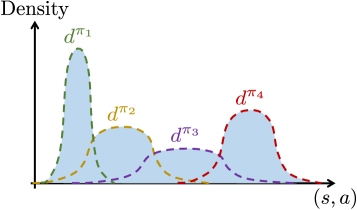
Figure 1: An example illustrating the equivalence of coverability and cumulative reachability. Here, $\Pi=\{\pi_{1},\pi_{2},\pi_{3},\pi_{4}\}$, and dashed curves plots $d^{\pi}$ for each $\pi\in\Pi$. The coverability coefficient, via Lemma 3, is equal to the total area of the shaded region (without double-counting overlapping regions).

The following lemma shows that cumulative reachability and coverability coincide; we defer the proof to Appendix A.

Lemma 3 (Equivalence of coverability and cumulative reachability).

The following definition is equivalent to Definition 2:

$$C_{\mathsf{cov}}\vcentcolon={}\max_{h\in[H]}\sum_{(x,a)\in\mathcal{X}\times\mathcal{A}}\sup_{\pi\in\Pi}d_{h}^{\pi}(x,a).$$

Equipped with Lemma 3, we proceed with the proof of Theorem 1.

Preliminaries

For each $t$, we define $\delta^{\scriptscriptstyle(t)}_{h}(\cdot,\cdot)\coloneqq f_{h}^{\scriptscriptstyle(t)}(\cdot,\cdot)-(\mathcal{T}_{h}f_{h+1}^{\scriptscriptstyle(t)})(\cdot,\cdot)$, which may be viewed as a “test function” at level $h$ induced by $f^{{\scriptscriptstyle(t)}}\in\mathcal{F}$. We adopt the shorthand $d_{h}^{\scriptscriptstyle(t)}\equiv{}d_{h}^{\pi^{\scriptscriptstyle(t)}}$, and we define

$$\widetilde{d}_{h}^{\scriptscriptstyle(t)}(x,a)\coloneqq~{}\sum_{i=1}^{t-1}d_{h}^{\scriptscriptstyle(i)}(x,a),\quad\text{and}\quad\mu^{\star}_{h}\coloneqq~{}\mathop{\mathrm{argmin}}_{\mu_{h}\in\Delta(\mathcal{X}\times\mathcal{A})}\sup_{\pi\in\Pi}\,\left\|\frac{d_{h}^{\pi}}{\mu_{h}}\right\|_{\infty}.$$ (1)

That is, $\widetilde{d}_{h}^{\scriptscriptstyle(t)}$ unnormalized average of all state visitations encountered prior to step $t$, and $\mu^{\star}_{h}$ is the distribution that attains the value of $C_{\mathsf{cov}}$ for layer $h$. Throughout the proof, we perform a slight abuse of notation and write ${\mathbb{E}}_{\widetilde{d}_{h}^{\scriptscriptstyle(t)}}[f]\coloneqq\sum_{i=1}^{t-1}{\mathbb{E}}_{d_{h}^{\scriptscriptstyle(i)}}[f]$ for any function $f:\mathcal{X}\times\mathcal{A}\to\mathbb{R}$.

Regret decomposition

As a consequence of completeness (Assumption 1) and the construction of $\mathcal{F}^{{\scriptscriptstyle(t)}}$, a standard concentration argument (Lemma 15 in Appendix A) guarantees that with probability at least $1-\delta$, for all $t\in[T]$:

$$\mathrm{(i)}\;\;Q^{\star}\in\mathcal{F}^{{\scriptscriptstyle(t)}},\quad\text{and}\quad\mathrm{(ii)}\;\;\sum_{x,a}\widetilde{d}_{h}^{\scriptscriptstyle(t)}(x,a)\left(\delta_{h}^{\scriptscriptstyle(t)}(x,a)\right)^{2}\leq O(\beta).$$ (2)

We condition on this event going forward. Since $Q^{\star}\in\mathcal{F}^{{\scriptscriptstyle(t)}}$, we are guaranteed that $f^{{\scriptscriptstyle(t)}}$ is optimistic (i.e., $f_{1}^{{\scriptscriptstyle(t)}}(x_{1},\pi_{f^{{\scriptscriptstyle(t)}},1}(x_{1}))\geq{}Q^{\star}_{1}(x_{1},\pi_{f^{\star},1}(x_{1}))$), and a regret decomposition for optimistic algorithms (Lemma 16 in Appendix A) allows us to relate regret to the average Bellman error under the learner’s sequence of policies:

$${\sf Reg}\leq{}\sum_{t=1}^{T}\left(f_{1}^{\scriptscriptstyle(t)}(x_{1},\pi_{f^{{\scriptscriptstyle(t)}}_{1},1}(x_{1}))-J(\pi^{{\scriptscriptstyle(t)}})\right)=\sum_{t=1}^{T}\sum_{h=1}^{H}{\mathbb{E}}_{(x,a)\sim{}d_{h}^{\scriptscriptstyle(t)}}\big{[}\underbrace{f_{h}^{{\scriptscriptstyle(t)}}(x,a)-(\mathcal{T}_{h}f_{h+1}^{{\scriptscriptstyle(t)}})(x,a)}_{=\vcentcolon\delta_{h}^{\scriptscriptstyle(t)}(x,a)}\big{]}.$$

To proceed, we use a change of measure argument to relate the on-policy average Bellman error ${\mathbb{E}}_{(x,a)\sim{}d_{h}^{\scriptscriptstyle(t)}}[\delta_{h}^{\scriptscriptstyle(t)}(x,a)]$ appearing above to the in-sample squared Bellman error ${\mathbb{E}}_{(x,a)\sim{}\widetilde{d}_{h}^{\scriptscriptstyle(t)}}[\delta_{h}^{\scriptscriptstyle(t)}(x,a)^{2}]$; the latter is small as a consequence of Eq. 2. Unfortunately, naive attempts at applying change-of-measure fail because during the initial rounds of exploration, the on-policy and in-sample visitation probabilities can be very different, making it impossible to relate the two quantities (i.e., any natural notion of extrapolation error will be arbitrarily large).

To address this issue, we introduce the notion of a “burn-in” phase for each state-action pair $(x,a)\in\mathcal{X}\times\mathcal{A}$ by defining

$$\tau_{h}(x,a)=\min\left\{t\mid\widetilde{d}_{h}^{\scriptscriptstyle(t)}(x,a)\geq C_{\mathsf{cov}}\cdot\mu^{\star}_{h}(x,a)\right\},$$

which captures the earliest time at which $(x,a)$ has been explored sufficiently; we refer to $t<\tau_{h}(x,a)$ as the burn-in phase for $(x,a)$.

Going forward, let $h\in[H]$ be fixed. We decompose regret into contributions from the burn-in phase for each state-action pair, and contributions from pairs which have been explored sufficiently and reached a stable phase “stable phase”.

$$\underbrace{\sum_{t=1}^{T}{\mathbb{E}}_{(x,a)\sim{}d_{h}^{\scriptscriptstyle(t)}}\left[\delta_{h}^{\scriptscriptstyle(t)}(x,a)\right]}_{\text{on-policy average Bellman error}}=\underbrace{\sum_{t=1}^{T}{\mathbb{E}}_{(x,a)\sim{}d_{h}^{\scriptscriptstyle(t)}}\left[\delta_{h}^{\scriptscriptstyle(t)}(x,a)\mathds{1}[t<\tau_{h}(x,a)]\right]}_{\text{burn-in phase}}+\underbrace{\sum_{t=1}^{T}{\mathbb{E}}_{(x,a)\sim{}d_{h}^{\scriptscriptstyle(t)}}\left[\delta_{h}^{\scriptscriptstyle(t)}(x,a)\mathds{1}[t\geq\tau_{h}(x,a)]\right]}_{\text{stable phase}}.$$

We will not show that every state-action pair leaves the burn-in phase. Instead, we use coverability to argue that the contribution from pairs that have not left this phase is small on average. In particular, we use that $\lvert\delta_{h}^{{\scriptscriptstyle(t)}}\rvert\leq{}1$ to bound

$$\sum_{t=1}^{T}{\mathbb{E}}_{(x,a)\sim{}d_{h}^{\scriptscriptstyle(t)}}\left[\delta_{h}^{\scriptscriptstyle(t)}(x,a)\mathds{1}[t<\tau_{h}(x,a)]\right]\leq\sum_{x,a}\sum_{t<\tau_{h}(x,a)}d_{h}^{\scriptscriptstyle(t)}(x,a)=\sum_{x,a}\widetilde{d}_{h}^{{\scriptscriptstyle(\tau_{h}(x,a))}}(x,a)\leq{}2C_{\mathsf{cov}}\sum_{x,a}\mu^{\star}_{h}(x,a)=2C_{\mathsf{cov}},$$

where the last inequality holds because

$$\widetilde{d}^{{\scriptscriptstyle(\tau_{h}(x,a))}}_{h}(x,a)=\widetilde{d}_{h}^{\scriptscriptstyle(\tau_{h}(x,a)-1)}(x,a)+d_{h}^{\scriptscriptstyle(\tau_{h}(x,a)-1)}(x,a)\leq 2C_{\sf cov}\cdot\mu_{h}^{\star}(x,a),$$

which follows from Eq. 1 and the definition of $\tau_{h}$.

For the stable phase, we apply change-of-measure as follows:

$$~{}\sum_{t=1}^{T}{\mathbb{E}}_{(x,a)\sim{}d_{h}^{\scriptscriptstyle(t)}}\left[\delta_{h}^{\scriptscriptstyle(t)}(x,a)\mathds{1}[t\geq\tau_{h}(x,a)]\right]$$

$$=~{}\sum_{t=1}^{T}\sum_{x,a}d_{h}^{\scriptscriptstyle(t)}(x,a)\left(\frac{\widetilde{d}_{h}^{\scriptscriptstyle(t)}(x,a)}{\widetilde{d}_{h}^{\scriptscriptstyle(t)}(x,a)}\right)^{\nicefrac{{1}}{{2}}}\delta_{h}^{\scriptscriptstyle(t)}(x,a)\mathds{1}[t\geq\tau_{h}(x,a)]$$

$$\leq~{}\underbrace{\sqrt{\sum_{t=1}^{T}\sum_{x,a}\frac{\left(\mathds{1}[t\geq\tau_{h}(x,a)]d_{h}^{\scriptscriptstyle(t)}(x,a)\right)^{2}}{\widetilde{d}_{h}^{\scriptscriptstyle(t)}(x,a)}}}_{\text{{\tt(I)}: extrapolation error}}\cdot\underbrace{\sqrt{\sum_{t=1}^{T}\sum_{x,a}\widetilde{d}_{h}^{\scriptscriptstyle(t)}(x,a)\left(\delta_{h}^{\scriptscriptstyle(t)}(x,a)\right)^{2}}}_{\text{{\tt(II)}: in-sample \emph{squared} Bellman error}},$$ (3)

where the last inequality is an application of Cauchy-Schwarz. Using part (II) of Eq. 2, we bound the in-sample error above by

$$\texttt{(II)}\leq O\big{(}\sqrt{\beta T}\big{)}.$$ (4)

Bounding the extrapolation error using coverability

To proceed, we show that the extrapolation error (I) is controlled by coverability. We begin with a scalar variant of the standard elliptic potential lemma (Lattimore and Szepesvári, 2020); this result is proven in Appendix A for completeness.

Lemma 4 (Per-state-action elliptic potential lemma).

Let $d^{\scriptscriptstyle(1)},d^{\scriptscriptstyle(2)},\dotsc,d^{\scriptscriptstyle(T)}$ be an arbitrary sequence of distributions over a set $\mathcal{Z}$ (e.g., $\mathcal{Z}=\mathcal{X}\times\mathcal{A}$), and let $\mu\in\Delta(\mathcal{Z})$ be a distribution such that $d^{\scriptscriptstyle(t)}(z)/\mu(z)\leq C$ for all $(z,t)\in\mathcal{Z}\times[T]$. Then for all $z\in\mathcal{Z}$, we have

$$\sum_{t=1}^{T}\frac{d^{\scriptscriptstyle(t)}(z)}{\sum_{i<t}d^{\scriptscriptstyle(i)}(z)+C\cdot\mu(z)}\leq O\left(\log\left(T\right)\right).$$

We bound the extrapolation error (I) by applying Lemma 4 on a per-state basis, then using coverability (and the equivalence to cumulative reachability) to argue that the potentials from different state-action pairs average out. Observe that by the definition of $\tau_{h}$, we have that for all $t\geq\tau_{h}(s,a)$, $\widetilde{d}_{h}^{\scriptscriptstyle(t)}(x,a)\geq C_{\sf cov}\mu_{h}^{\star}(x,a)\Rightarrow\widetilde{d}_{h}^{\scriptscriptstyle(t)}(x,a)\geq\frac{1}{2}(\widetilde{d}_{h}^{\scriptscriptstyle(t)}(x,a)+C_{\sf cov}\mu_{h}^{\star}(x,a))$, which allows us to bound term (I) of extrapolation error by

$$\sum_{t=1}^{T}\sum_{x,a}\frac{\left(\mathds{1}[t\geq\tau_{h}(x,a)]d_{h}^{\scriptscriptstyle(t)}(x,a)\right)^{2}}{\widetilde{d}_{h}^{\scriptscriptstyle(t)}(x,a)}\leq ~{}2\sum_{t=1}^{T}\sum_{x,a}\frac{d_{h}^{\scriptscriptstyle(t)}(x,a)\cdot d_{h}^{\scriptscriptstyle(t)}(x,a)}{\widetilde{d}_{h}^{\scriptscriptstyle(t)}(x,a)+C_{\sf cov}\cdot\mu_{h}^{\star}(x,a)}$$

$$\leq ~{}2\sum_{t=1}^{T}\sum_{x,a}\max_{t^{\prime}\in[T]}d_{h}^{{\scriptscriptstyle(t^{\prime})}}(x,a)\cdot\frac{d_{h}^{\scriptscriptstyle(t)}(x,a)}{\widetilde{d}_{h}^{\scriptscriptstyle(t)}(x,a)+C_{\sf cov}\cdot\mu_{h}^{\star}(x,a)}$$

$$\leq ~{}2\underbrace{\left(\max_{(s,a)\in\mathcal{S}\times\mathcal{A}}\sum_{t=1}^{T}\frac{d_{h}^{\scriptscriptstyle(t)}(x,a)}{\widetilde{d}_{h}^{\scriptscriptstyle(t)}(x,a)+C_{\sf cov}\cdot\mu_{h}^{\star}(x,a)}\right)}_{\leq O(\log(T))\text{ by \lx@cref{creftype~refnum}{lem:per_sa_ep}}}\cdot\underbrace{\left(\sum_{x,a}\max_{t\in[T]}d^{{\scriptscriptstyle(t)}}_{h}(x,a)\right)}_{\leq C_{\sf cov}\text{ by \lx@cref{creftype~refnum}{lem:concen_eq_area}}}$$

$$\leq ~{}O\left(C_{\sf cov}\log\left(T\right)\right).$$ (5)

To conclude, we substitute Eqs. 4 and 5 into Eq. 3, which gives

$${\sf Reg}\leq\sum_{h=1}^{H}{\mathbb{E}}_{(x,a)\sim{}d_{h}^{\scriptscriptstyle(t)}}\left[\delta_{h}^{\scriptscriptstyle(t)}(x,a)\right]\leq O\left(H\sqrt{C_{\mathsf{cov}}\cdot\beta T\log(T)}\right).$$

∎

To obtain the expression in Eq. 3 (term (I)), our proof critically uses that the confidence set construction provides a bound on the squared Bellman error ${\mathbb{E}}_{(x,a)\sim{}\widetilde{d}_{h}^{\scriptscriptstyle(t)}}[\delta_{h}^{\scriptscriptstyle(t)}(x,a)^{2}]$ in the change of measure argument. This contrasts with existing works on online RL with general function approximation (e.g., Jiang et al., 2017; Jin et al., 2021a; Du et al., 2021), which typically move from average Bellman error to squared Bellman error as a lossy step, and only work with squared Bellman error because it permits simpler construction of confidence sets. For the argument in Eq. 3, confidence sets based on average Bellman error will lead to a larger notion of extrapolation error which cannot be controlled using coverability (cf. Section 5).

3.3 Rich Observations and Exogenous Noise: Application to Block MDPs

As an application of Theorem 1, we consider the problem of reinforcement learning in Exogenous Block MDPs (Ex-BMDPs), a problem which has received extensive recent interest (Efroni et al., 2021, 2022a, 2022b; Lamb et al., 2022). Recall that the block MDP (Jiang et al., 2017; Du et al., 2019; Misra et al., 2020) is a model in which the (“observed”) state space $\mathcal{X}$ is large/high-dimensional, but the dynamics are governed by a (small) latent state space. Exogenous block MDPs generalize this model further by factorizing the latent state space into small controllable (“endogenous”) component and a large irrelevant (“exogenous”) component, which may be temporally correlated.

Following Efroni et al. (2021), an Ex-BMDP $M=(\mathcal{X},\mathcal{A},P,R,H,x_{1})$ is defined by an (unobserved) latent state space, which consists of an endogenous state $s_{h}\in\mathcal{S}$ and exogenous state $\xi_{h}\in\Xi$, and an observation process which generates the observed state $x_{h}$. We first describe the dynamics for the latent space. Given initial endogenous and exogenous states $s_{1}\in\mathcal{S}$ and $\xi_{1}\in\Xi$, the latent states evolve via

$$s_{h+1}\sim{}P^{\mathrm{endo}}_{h}(s_{h},a_{h}),\quad\text{and}\quad\xi_{h+1}\sim P^{\mathrm{exo}}_{h}(\xi_{h});$$

that is while both states evolve in a temporally correlated fashion, only the endogenous state $s_{h}$ evolves as a function of the agent’s action. The latent state $(s_{h},\xi_{h})$ is not observed. Instead, we observe

$$x_{h}\sim{}q_{h}(s_{h},\xi_{h}),$$

where $q_{h}:\mathcal{S}\times\Xi\to\Delta(\mathcal{X})$ is an emission distribution with the property that $\mathrm{supp}(q_{h}(s,\xi))\cap\mathrm{supp}(q_{h}(s^{\prime},\xi^{\prime}))=\varnothing$ if $(s,\xi)\neq(s^{\prime},\xi^{\prime})$. This property (decodability) ensures that there exists a unique mapping $\phi^{\star}_{h}:\mathcal{X}\to\mathcal{S}$ that maps the observed state $x_{h}$ to the corresponding endogenous latent state $s_{h}$. We assume that $R_{h}(x,a)=R_{h}(\phi^{\star}_{h}(x),a)$, which implies that optimal policy $\pi^{\star}$ depends only on the endogenous latent state, i.e. $\pi^{\star}_{h}(x)=\pi^{\star}_{h}(\phi^{\star}_{h}(x))$.

The main challenge of learning in block MDPs is that the decoder $\phi^{\star}$ is not known to the learner in advance. Indeed, given access to the decoder, one can obtain regret $\mathrm{poly}(H,\lvert\mathcal{S}\rvert,\lvert\mathcal{A}\rvert)\cdot\sqrt{T}$ by applying tabular reinforcement learning algorithms to the latent state space. In light of this, the aim of the Ex-BMDP setting is to obtain sample complexity guarantees that are independent of the size of the observed state space $\lvert\mathcal{X}\rvert$ and exogenous state space $\lvert\Xi\rvert$, and scale as $\mathrm{poly}(\lvert\mathcal{S}\rvert,\lvert\mathcal{A}\rvert,H,\log\lvert\mathcal{F}\rvert)$, where $\mathcal{F}$ is an appropriate class of function approximators (typically either a value function class $\mathcal{F}$ or a class of decoders $\Phi$ that attempts to model $\phi^{\star}$ directly).

Ex-BMDPs present substantial additional difficulties compared to classical block MDPs because we aim to avoid dependence on the size $\lvert\Xi\rvert$ of the exogenous latent state space. Here, the main challenge is that executing policies $\pi$ whose actions depend on $\xi_{h}$ can lead to spurious correlations between endogenous exogenous states. In spite of this apparent difficulty, we show that the coverability coefficient for this setting is always bounded by the number of endogenous states.

Proposition 5.

For any Ex-BMDP, $C_{\mathsf{cov}}\leq\lvert\mathcal{S}\rvert\cdot\lvert\mathcal{A}\rvert$.

This bound is a consequence of a structural result from Efroni et al. (2021), which shows that for any $(s,a)\in\mathcal{S}\times\mathcal{A}$, all $x\in\mathcal{X}$ with $\phi^{\star}(x)=s$ admit a common policy that maximizes $d_{h}^{\pi}(x,a)$, and this policy is endogenous, i.e., only depends on the endogenous state $s_{h}=\phi^{\star}_{h}(x_{h})$. As a corollary, we obtain the following regret bound.

Corollary 6.

For the Ex-BMDP setting, under Assumption 1, Algorithm 1 ensures that with probability at least $1-\delta$,

$${\sf Reg}\leq O\big{(}H\sqrt{\lvert\mathcal{S}\rvert\lvert\mathcal{A}\rvert T\log(\nicefrac{{TH|\mathcal{F}|}}{{\delta}})\log(T)}\big{)}.$$

Critically, this result scales only with the cardinality $\lvert\mathcal{S}\rvert$ for the endogenous latent state space, and with the capacity $\log\lvert\mathcal{F}\rvert$ for the value function class.

Corollary 6 is the first result for this setting that allows for stochastic latent dynamics and emission process, albeit with the extra assumption of completeness. Existing algorithms either require that the endogenous latent dynamics $P^{\mathrm{endo}}$ are deterministic (Efroni et al., 2021) or allow for stochastic dynamics but heavily restrict the observation process (Efroni et al., 2022a); complexity measures such as Bellman Rank and Bellman-Eluder dimension can be arbitrarily large (see discussion in Section 5). Our result is best thought of as a “luckiness” guarantee, in the sense that it is unclear how to construct a value function class that is complete for every problem instance, but the algorithm will succeed whenever $\mathcal{F}$ does happen to be complete for a given instance. Understanding whether general Ex-BMDPs are learnable without completeness is an interesting question for future work, and we are hopeful that the perspective of coverability will lead to further insights for this setting.

Invariance of coverability

Proposition 5 is a consequence of two general invariance properties of coverability, which show that $C_{\mathsf{cov}}$ is unaffected by the following augmentations to the underlying MDP: (i) addition of rich observations, and (ii) addition of exogenous noise.

The first property shows that for a given MDP $M$, creating a new block MDP $M^{\prime}$ by equipping $M$ with a decodable emission process (so that $M$ acts as a latent MDP), does not increase coverability.

Proposition 7 (Invariance to rich observations).

Let an MDP $M=(\mathcal{S},\mathcal{A},P,R,H,s_{1})$. Let $M^{\prime}=(\mathcal{X},\mathcal{A},P^{\prime},R^{\prime},H,x_{1})$ be the MDP defined implicitly by the following process. For each $h\in\left[H\right]$:

• $s_{h+1}\sim{}P_{h}(s_{h},a_{h})$ and $r_{h}=R_{h}(s_{h},a_{h})$. Here, $s_{h}$ is unobserved, and may be thought of as a latent state.

• $x_{h}\sim{}q_{h}(s_{h})$, where $q_{h}:\mathcal{S}\to\Delta(\mathcal{X})$ is an emission distribution with the property that $\mathrm{supp}(q_{h}(s))\cap\mathrm{supp}(q_{h}(s^{\prime}))=\varnothing$ for $s\neq{}s^{\prime}$.

Then, writing $C_{\mathsf{cov}}(M)$ to make the dependence on $M$ explicit, we have

$$C_{\mathsf{cov}}(M^{\prime})\leq C_{\mathsf{cov}}(M).$$

The second result shows that coverability is also preserved if we expand the state space to include temporally correlated exogenous state whose evolution does not depend on the agent’s actions.

Proposition 8 (Invariance to exogenous noise).

Let an MDP $M=(\mathcal{S},\mathcal{A},P,R,H,s_{1})$, conditional distribution $P^{\mathrm{exo}}:\Xi\to\Delta(\Xi)$, and $\xi_{1}\in\Xi$ be given, where $\Xi$ is an abstract set. Let $\mathcal{X}\vcentcolon={}\mathcal{S}\times\Xi$, and let $M^{\prime}=(\mathcal{X},\mathcal{A},P^{\prime},R^{\prime},H,x_{1})$ be the MDP with state $x_{h}=(s_{h},\xi_{h})$ defined implicitly by the following process. For each $h\in[H]$:

• $s_{h+1}\sim{}P_{h}(s_{h},a_{h})$, $r_{h}=R_{h}(s_{h},a_{h})$.

• $\xi_{h+1}\sim{}P^{\mathrm{exo}}_{h}(\xi_{h})$.

Then we have

$$C_{\mathsf{cov}}(M^{\prime})\leq C_{\mathsf{cov}}(M).$$

This result is non-trivial because policies that act based on the endogenous state $s_{h}$ and $\xi_{h}$ can cause these processes to become coupled (Efroni et al., 2021), but holds nonetheless.

Proposition 5 can be deduced by combining Propositions 7 and 8 with the observation that any tabular (finite-state/action) MDP with $S$ states and $A$ actions has $C_{\mathsf{cov}}\leq{}SA$. However, Propositions 7 and 8 yield more general results, since they imply that starting with any (potentially non-tabular) class of MDPs $\mathcal{M}$ with low coverability and augmenting it with rich observations and exogenous noise preserves coverability.

4 Are Weaker Notions of Coverage Sufficient?

In Section 3, we showed that existence of a distribution with good concentrability (coverability) is sufficient for sample-efficient online RL. However, while concentrability is the most ubiquitous coverage condition in offline RL, there are several weaker notions of coverage which also lead to sample-efficient offline RL algorithms. In this section, we show that analogues of coverability based on these conditions, single-policy concentrability and generalized concentrability for Bellman residuals, do not suffice for sample-efficient online RL. This indicates that in general, the interplay between offline coverage and online exploration is nuanced.

Single-policy concentrability

Single-policy concentrability is a widely used coverage assumption in offline RL which weakens concentrability by requiring only that the state distribution induced by $\pi^{\star}$ is covered by the offline data distribution $\mu$, as opposed to requiring coverage for all policies (Jin et al., 2021b; Rashidinejad et al., 2021).

Definition 3 (Single-policy concentrability).

The single-policy concentrability coefficient for a data distribution $\mu=\left\{\mu_{h}\right\}_{h=1}^{H}$ is given by

$$C_{\mathsf{conc}}^{\star}(\mu)\vcentcolon={}\left\|\frac{d_{h}^{\pi^{\star}}}{\mu_{h}}\right\|_{\infty}.$$

For offline RL, algorithms based on pessimism provide sample guarantee complexity guarantees that scale with $C_{\mathsf{conc}}^{\star}(\mu)$ (Jin et al., 2021b; Rashidinejad et al., 2021). However, for the online setting, it is trivial to show that an analogous notion of “single-policy coverability” (i.e., existence of a distribution with good single-policy coverability) is not sufficient for sample-efficient learning, since for any MDP, one can take $\mu=d^{\pi^{\star}}$ to attain $C_{\mathsf{conc}}^{\star}(\mu)=1$. This suggests that any notion of coverage that suffices for online RL must be more uniform in nature.

Generalized concentrability for Bellman residuals

Another approach to weaker coverage in offline RL is to relaxed concentrability by only requiring coverage with respect to the Bellman residuals for value functions in $\mathcal{F}$ (Chen and Jiang, 2019; Xie et al., 2021a; Cheng et al., 2022); the following definition adapts this notion to the finite-horizon setting.

Definition 4 (Generalized concentrability).

We define the generalized concentrability coefficient $\mathfrak{C}_{\mathsf{conc}}(\mu,\mathcal{F})$ for a policy class $\Pi$ and value function class $\mathcal{F}$ as the least constant $C>0$ such that the offline data distribution $\mu=\left\{\mu_{h}\right\}_{h=1}^{H}$ satisfies that for all $f\in\mathcal{F}$ and $\pi\in\Pi$,

$$\sum_{h=1}^{H}{\mathbb{E}}_{d_{h}^{\pi}}\left[\left(f_{h}(s_{h},a_{h})-(\mathcal{T}_{h}f_{h+1})(s_{h},a_{h})\right)^{2}\right]\leq C\cdot\sum_{h=1}^{H}{\mathbb{E}}_{\mu_{h}}\left[\left(f_{h}(s_{h},a_{h})-(\mathcal{T}_{h}f_{h+1})(s_{h},a_{h})\right)^{2}\right].$$

Note that $\mathfrak{C}_{\sf conc}(\mu,\mathcal{F})\leq C_{\mathsf{conc}}(\mu)$ (in particular, they coincide if one chooses $\mathcal{F}$ to be the set of all functions over $\mathcal{X}\times\mathcal{A}$) but in general $\mathfrak{C}_{\sf conc}(\mu,\mathcal{F})$ can be much smaller. For example, in the linear Bellman-complete setting, it is possible to bound $\mathfrak{C}_{\sf conc}(\mu,\mathcal{F})$ in terms of feature coverage conditions (Wang et al., 2021a; Zanette et al., 2021). Using offline data from $\mu$, sample complexity guarantees that scale with $\mathfrak{C}_{\sf conc}(\mu,\mathcal{F})$ can be obtained under Assumption 1 via MSBO (see, e.g., Xie and Jiang, 2020, Section 5) or by running a “one-step” variant of Golf (Algorithm 1); we provide this result (Proposition 17) in Appendix B for completeness. Given that this notion leads to positive results for offline RL, it is natural to consider a generalized notion of coverability based upon it.

Definition 5 (Generalized coverability).

We define the generalized coverability coefficient for a policy class $\Pi$ value function class $\mathcal{F}$ and as

$$\mathfrak{C}_{\mathsf{cov}}(\mathcal{F})=\inf_{\mu_{1},\ldots,\mu_{H}\in\Delta(\mathcal{X}\times\mathcal{A})}\{\mathfrak{C}_{\mathsf{conc}}(\mu,\mathcal{F})\}.$$

Unfortunately, we show that this condition does not suffice for sample-efficient online RL, even when the number of actions is constant and Assumption 1 is satisfied.

Theorem 9.

For any $X,H,C\in\mathbb{N}$, there exists a family of MDPs with $\lvert\mathcal{X}\rvert=X$, $|\mathcal{A}|=2$ and horizon $H$ and a function class $\mathcal{F}$ with $\log\lvert\mathcal{F}\rvert\leq{}H\log(2\lvert\mathcal{X}\rvert)$ such that: i) Assumption 1 (completeness) is satisfied for $\mathcal{F}$ and we have $\mathfrak{C}_{\sf cov}(\mathcal{F})\leq{}C$ and ii) Any online RL algorithm that returns a $0.1$-optimal policy with probability $0.9$ requires at least

$$\Omega\left(\min\left\{X,2^{\Omega(H)},2^{\Omega(C)}\right\}\right)$$

trajectories.

Theorem 9 highlights that in general, notions of coverage that suffice for offline RL—even those that are uniform in nature—can fail to lead to useful structural conditions for online RL. Briefly, the issue is that bounding regret for online RL entails controlling the extent to which a deliberate algorithm that has observed state distributions $d_{h}^{\pi^{{\scriptscriptstyle(1)}}},\ldots,d_{h}^{\pi^{{\scriptscriptstyle(t-1)}}}$ can be “surprised” by a substantially new state distribution $d_{h}^{\pi^{{\scriptscriptstyle(t)}}}$; here, surprise is typically measure in terms of Bellman residual. The proof of Theorem 9 shows that existence of a distribution with good coverage with respect to Bellman residuals does suffice to provide meaningful control of distribution shift. We caution, however, that the lower bound construction makes use of the fact that Definition 5 requires coverage only on average across layers, and it is unclear whether a similar lower bound holds under uniform coverage across layers. Developing a more unified and fine-grained understanding of what coverage conditions lead to efficient exploration is an important question for future research.

5 A New Structural Condition for Sample-Efficient Online RL

Having shown that coverability serves a structural condition that facilitates sample-efficient online reinforcement learning, an immediate question is whether this structural condition is related to existing complexity measures such as Bellman-Eluder dimension (Jin et al., 2021a) and Bellman/Bilinear rank (Jiang et al., 2017; Du et al., 2021), which attempt to unify existing approaches to sample-efficient RL. We now show that these complexity measures are insufficient to capture coverability, then provide a new complexity measure, the Sequential Extrapolation Coefficient, which bridges the gap.

5.1 Insufficiency of Existing Complexity Measures

Bellman-Eluder dimension (Jin et al., 2021a) and Bellman/Bilinear rank (Jiang et al., 2017; Du et al., 2021) can fail to capture coverability for two reasons: (i) insufficiency of average Bellman error (as opposed to squared Bellman error), and (ii) incorrect dependence on scale. To highlight these issues, we focus on $Q$-type Bellman-Eluder dimension (Jin et al., 2021a), which subsumes Bellman rank. See Appendix C for discussion of other complexity measures, including Bilinear rank.

Let $\mathfrak{D}_{h}^{\Pi}\coloneqq\{d^{\pi}_{h}:\pi\in\Pi\}$ and $\mathcal{F}_{h}-\mathcal{T}_{h}\mathcal{F}_{h+1}\coloneqq\{f_{h}-\mathcal{T}_{h}f_{h+1}:f\in\mathcal{F}\}$. Following Jin et al. (2021a), we define the ($Q$-type) Bellman-Eluder dimension as follows.

Definition 6 (Bellman-Eluder dimension).

The Bellman-Eluder dimension $\mathsf{dim}_{\mathsf{BE}}(\mathcal{F},\Pi,\varepsilon,h)$ for the layer $h$ is the largest $d\in\mathbb{N}$, such that there exist sequences $\{d_{h}^{\scriptscriptstyle(1)},d_{h}^{\scriptscriptstyle(2)},\dotsc,d_{h}^{\scriptscriptstyle(d)}\}\subseteq\mathfrak{D}^{\Pi}_{h}$ and $\{\delta_{h}^{{\scriptscriptstyle(1)}},\ldots,\delta_{h}^{\scriptscriptstyle(d)}\}\subseteq\mathcal{F}_{h}-\mathcal{T}_{h}\mathcal{F}_{h+1}$ such that for all $t\in[d]$,,

$$\lvert{\mathbb{E}}_{d_{h}^{\scriptscriptstyle(t)}}[\delta_{h}^{\scriptscriptstyle(t)}]\rvert>\varepsilon^{\scriptscriptstyle(t)},\quad\text{and}\quad\sqrt{\sum_{i=1}^{t-1}\big{(}{\mathbb{E}}_{d_{h}^{\scriptscriptstyle(i)}}[\delta_{h}^{\scriptscriptstyle(t)}]\big{)}^{2}}\leq\varepsilon^{\scriptscriptstyle(t)},$$ (6)

for $\varepsilon^{{\scriptscriptstyle(1)}},\ldots,\varepsilon^{{\scriptscriptstyle(d)}}\geq\varepsilon$. We define $\mathsf{dim}_{\mathsf{BE}}(\mathcal{F},\Pi,\varepsilon)=\max_{h\in[H]}\mathsf{dim}_{\mathsf{BE}}(\mathcal{F},\Pi,\varepsilon,h)$.

Issue #1: Insufficiency of average (vs. squared) Bellman error

The Bellman-Eluder dimension reflects the length of the longest consecutive sequence of value function pairs for which we can be “surprised” by a large Bellman residual for a new policy if the value function has low Bellman residual on all preceding policies. Note that via Eq. 6, the Bellman-Eluder dimension measures the size of the surprise and the error on preceding points via average Bellman error (e.g., ${\mathbb{E}}_{d_{h}^{\scriptscriptstyle(i)}}[\delta_{h}^{\scriptscriptstyle(t)}]$). On the other hand, the proof of Theorem 1 critically uses squared Bellman error ${\mathbb{E}}_{d_{h}^{\scriptscriptstyle(i)}}[(\delta_{h}^{\scriptscriptstyle(t)})^{2}]$ bound regret by coverability; this is because the (point-wise) nonnegativity of squared Bellman error facilitates change-of-measure in a similar fashion to offline reinforcement learning. The following result shows that this issue is fundamental, and Bellman-Eluder dimension can be exponential large relative to the regret bound in Theorem 1.

Proposition 10.

For any $d\in\mathbb{N}$, there exists an MDP $M$ with $H=2$ and $\lvert\mathcal{A}\rvert=2$, policy class $\Pi$ with $\lvert\Pi\rvert=d$, and value function class $\mathcal{F}$ with $\lvert\mathcal{F}\rvert=d$ satisfying completeness, such that $C_{\sf cov}=O(1)$, but the Bellman-Eluder dimension has $\mathsf{dim}_{\mathsf{BE}}(\mathcal{F},\Pi,\varepsilon)=\Omega(\min\{|\mathcal{F}|,|\Pi|\})=\Omega(d)$ for any $\varepsilon\leq 1/2$.

The lower bound in Proposition 10 is realized by an exogenous block MDP (Section 3.3), with $d$ representing the number of exogenous states. The result gives an exponential separation between what can be achieved using Bellman-Eluder dimension and coverability, because Golf attains ${\sf Reg}\leq\widetilde{O}\big{(}\sqrt{T\log(d)}\big{)}$ (cf. Corollary 6), yet we have $\mathsf{dim}_{\mathsf{BE}}(\mathcal{F},\Pi,1/2)=\Omega(d)$. This exponential separation can also be shown to apply to algorithms based on average Bellman error: Proposition 18 (Appendix C) shows that Olive (Jiang et al., 2017) requires $\Omega(d)$ trajectories to obtain a near-optimal policy. The construction, which is based on Efroni et al. (2022b, Section B.1), critically leverages cancellations in the average Bellman error; these cancellations are ruled out by squared Bellman error, which is why Theorem 1 gives a regret bound that scales only logarithmically in $d$. Bilinear rank (Du et al., 2021) and $V$-type Bellman rank suffer from similar drawbacks; see Appendix C for further discussion.

Issue #2: Incorrect dependence on scale

In light of the previous example, a seemingly reasonable fix is to adapt the Bellman-Eluder dimension to consider squared Bellman error rather than average Bellman error. Consider the following variant.

Definition 7 (Squared Bellman-Eluder dimension).

We define the Squared Bellman-Eluder dimension $\mathsf{dim}_{\mathsf{BE}}^{\mathsf{sq}}(\mathcal{F},\Pi,\varepsilon,h)$ for layer $h$ is the largest $d\in\mathbb{N}$ such that there exist sequences $\{d_{h}^{\scriptscriptstyle(1)},d_{h}^{\scriptscriptstyle(2)},\dotsc,d_{h}^{\scriptscriptstyle(d)}\}\subseteq\mathfrak{D}^{\Pi}_{h}$ and $\{\delta_{h}^{{\scriptscriptstyle(1)}},\ldots,\delta_{h}^{\scriptscriptstyle(d)}\}\subseteq\mathcal{F}_{h}-\mathcal{T}_{h}\mathcal{F}_{h+1}$ such that for all $t\in[d]$,

$$\lvert{\mathbb{E}}_{d_{h}^{\scriptscriptstyle(t)}}[\delta_{h}^{\scriptscriptstyle(t)}]\rvert>\varepsilon^{\scriptscriptstyle(t)},\quad\text{and}\quad\sqrt{\sum_{i=1}^{t-1}{\mathbb{E}}_{d_{h}^{\scriptscriptstyle(i)}}[(\delta_{h}^{\scriptscriptstyle(t)})^{2}]}\leq\varepsilon^{\scriptscriptstyle(t)},$$ (7)

for $\varepsilon^{{\scriptscriptstyle(1)}},\ldots,\varepsilon^{{\scriptscriptstyle(d)}}\geq\varepsilon$. We define $\mathsf{dim}_{\mathsf{BE}}^{\mathsf{sq}}(\mathcal{F},\Pi,\varepsilon)=\max_{h\in[H]}\mathsf{dim}_{\mathsf{BE}}^{\mathsf{sq}}(\mathcal{F},\Pi,\varepsilon,h)$.

This definition is identical to Definition 6, except that the constraint $\sqrt{\sum_{i=1}^{t-1}({\mathbb{E}}_{d_{h}^{\scriptscriptstyle(i)}}[\delta_{h}^{\scriptscriptstyle(t)}])^{2}}\leq\varepsilon^{\scriptscriptstyle(t)}$ in Eq. 6 has been replaced by the constraint $\sqrt{\sum_{i=1}^{t-1}{\mathbb{E}}_{d_{h}^{\scriptscriptstyle(i)}}[(\delta_{h}^{\scriptscriptstyle(t)})^{2}]}\leq\varepsilon^{\scriptscriptstyle(t)}$, which uses squared Bellman error instead of average Bellman error. By adapting the analysis of Jin et al. (2021a) it is possible to show that this definition yields ${\sf Reg}\leq\widetilde{O}\big{(}H\sqrt{\inf_{\varepsilon>0}\{\varepsilon^{2}T+\mathsf{dim}_{\mathsf{BE}}^{\mathsf{sq}}(\mathcal{F},\Pi,\varepsilon)\}\cdot{}T\log\lvert\mathcal{F}\rvert}\big{)}$. If one could show that $\mathsf{dim}_{\mathsf{BE}}^{\mathsf{sq}}(\mathcal{F},\Pi,\varepsilon)\lesssim{}C_{\mathsf{cov}}\cdot\mathrm{polylog}(\varepsilon^{-1})$, this would recover Theorem 1. Unfortunately, it turns out that in general, one can have $\mathsf{dim}_{\mathsf{BE}}^{\mathsf{sq}}(\mathcal{F},\Pi,\varepsilon)=\Omega(C_{\mathsf{cov}}/\varepsilon)$, which leads to suboptimal $T^{2/3}$-type regret using the result above. The following result shows that this guarantee cannot be improved without changing the complexity measure under consideration.

Proposition 11.

Fix $T\in\mathbb{N}$, and let $\varepsilon_{T}\vcentcolon={}T^{-1/3}$. There exist MDP class/policy class/value function class tuples $(\mathcal{M}_{1},\Pi_{1},\mathcal{F}_{1})$ and $(\mathcal{M}_{2},\Pi_{2},\mathcal{F}_{2})$ with the following properties.

1. All MDPs in $\mathcal{M}_{1}$ (resp. $\mathcal{M}_{2}$) satisfy Assumption 1 with respect to $\mathcal{F}_{1}$ (resp. $\mathcal{F}_{2}$). In addition, $\log\lvert\mathcal{F}_{1}\rvert=\log\lvert\mathcal{F}_{2}\rvert=\widetilde{O}(1)$.

2. For all MDPs in $\mathcal{M}_{1}$, we have $\mathsf{dim}_{\mathsf{BE}}^{\mathsf{sq}}(\mathcal{F}_{1},\Pi_{1},\varepsilon_{T})\propto{}1/\varepsilon_{T}$, and any algorithm must have $\operatorname{\mathbb{E}}\left[{\sf Reg}\right]\geq{}\Omega(T^{2/3})$ for some MDP in the class

3. For all MDPs in $\mathcal{M}_{2}$, we also have $\mathsf{dim}_{\mathsf{BE}}^{\mathsf{sq}}(\mathcal{F}_{2},\Pi_{2},\varepsilon_{T})\propto{}1/\varepsilon_{T}$, yet $C_{\mathsf{cov}}=O(1)$ and Golf attains $\operatorname{\mathbb{E}}\left[{\sf Reg}\right]\leq\widetilde{O}(\sqrt{T})$.

This result shows that there are two classes for which the optimal rate differs polynomially ($\Omega(T^{2/3})$ vs. $\widetilde{O}(\sqrt{T})$), yet the Bellman-Eluder dimension has the same size, and implies that the Bellman-Eluder dimension cannot provide rates better than $\Omega(T^{2/3})$ for classes with low coverability in general. Informally, the reason why Bellman-Eluder dimension fails capture the optimal rates for the problem instances in Proposition 11 is that the definition in Eq. 7 only checks whether the average Bellman error violates the threshold $\varepsilon$, and does not consider how far the error violates the threshold ($\lvert{\mathbb{E}}_{d_{h}^{\scriptscriptstyle(t)}}[\delta_{h}^{\scriptscriptstyle(t)}]\rvert>\varepsilon$ and $\lvert{\mathbb{E}}_{d_{h}^{\scriptscriptstyle(t)}}[\delta_{h}^{\scriptscriptstyle(t)}]\rvert>1$ are counted the same).

5.2 The Sequential Extrapolation Coefficient

To address the issues above, we introduce a new complexity measure, the Sequential Extrapolation Coefficient ($\mathsf{SEC}$), which i) leads to regret bounds via Golf and ii) subsumes both coverability and the Bellman-Eluder dimension. Conceptually, the Sequential Extrapolation Coefficient should be thought of as a minimal abstraction of the main ingredient in regret bounds based on Golf and other optimistic algorithms: extrapolation from in-sample error to on-policy error. We begin by stating a variant of the Sequential Extrapolation Coefficient for abstract function classes, then specialize it to reinforcement learning.

Definition 8 (Sequential Extrapolation Coefficient).

Let $\mathcal{Z}$ be an abstract set. Given a test function class $\Psi\subset(\mathcal{Z}\to\mathbb{R})$ and distribution class $\mathfrak{D}\subset\Delta(\mathcal{Z})$, the sequential extrapolation coefficient for length $T$ is given by

$$\mathsf{SEC}(\Psi,\mathfrak{D},T)\vcentcolon={}\sup_{\{\psi^{{\scriptscriptstyle(1)}},\ldots,\psi^{{\scriptscriptstyle(T)}}\}\subseteq\Psi}\sup_{\{d^{{\scriptscriptstyle(1)}},\ldots,d^{{\scriptscriptstyle(T)}}\}\subseteq\mathfrak{D}}\left\{\sum_{t=1}^{T}\frac{{\mathbb{E}}_{d^{{\scriptscriptstyle(t)}}}[\psi^{{\scriptscriptstyle(t)}}]^{2}}{1\vee\sum_{i=1}^{t-1}{\mathbb{E}}_{d^{{\scriptscriptstyle(i)}}}[(\psi^{{\scriptscriptstyle(t)}})^{2}]}\right\}.$$

To apply the Sequential Extrapolation Coefficient to RL, we use Bellman residuals for $\mathcal{F}$ as test functions and consider state-action distributions induced by policies in $\Pi$.

Definition 9 ($\mathsf{SEC}$ for RL).

We define

For each $h\in[H]$, let $\mathfrak{D}_{h}^{\Pi}\coloneqq\{d^{\pi}_{h}:\pi\in\Pi\}$ and $\mathcal{F}_{h}-\mathcal{T}_{h}\mathcal{F}_{h+1}\coloneqq\{f_{h}-\mathcal{T}_{h}f_{h+1}:f\in\mathcal{F}\}$. We define

$$\mathsf{SEC}_{\mathsf{RL}}(\mathcal{F},\Pi,T)\coloneqq\max_{h\in[H]}\mathsf{SEC}(\mathcal{F}_{h}-\mathcal{T}_{h}\mathcal{F}_{h+1},\mathfrak{D}_{h}^{\Pi},T).$$

The following result, which is a near-immediate consequence of the definition, shows that the Sequential Extrapolation Coefficient leads to regret bounds via Golf; recall that $\Pi=\{\pi_{f}\mid{}f\in\mathcal{F}\}$ is the set of greedy policies induced by $\mathcal{F}$.

Theorem 12.

Under Assumption 1, there exists an absolute constant $c$ such that for any $\delta\in(0,1]$ and $T\in\mathbb{N}_{+}$, if we choose $\beta=c\cdot\log(\nicefrac{{TH|\mathcal{F}|}}{{\delta}})$ in Algorithm 1, then with probability at least $1-\delta$, we have

$${\sf Reg} \leq O\left(H\sqrt{\mathsf{SEC}_{\mathsf{RL}}(\mathcal{F},\Pi,T)\cdot{}T\cdot\log(\nicefrac{{TH|\mathcal{F}|}}{{\delta}})}\right).$$

We defer the proof of Theorem 12 to Appendix C, and conclude by showing that the Sequential Extrapolation Coefficient subsumes coverability and Bellman-Eluder dimension.

Proposition 13 (Coverability $\Longrightarrow$ $\mathsf{SEC}$).

Let $C_{\sf cov}$ be the coverability coefficient (Definition 2) for policy class $\Pi$. Then for any value function class $\mathcal{F}$, $\mathsf{SEC}_{\mathsf{RL}}(\mathcal{F},\Pi,T)\leq O\left(C_{\sf cov}\cdot\log(T)\right)$.

Proposition 14 (Bellman-Eluder dimension $\Longrightarrow$ $\mathsf{SEC}$).

Suppose $\mathsf{dim}_{\mathsf{BE}\text{-}\mathsf{v}}(\mathcal{F},\Pi,\varepsilon)$ be Bellman-Eluder dimension (Definition 6) with function class $\mathcal{F}$ and policy $\Pi$, then

$$\mathsf{SEC}_{\mathsf{RL}}(\mathcal{F},\Pi,T)\leq O\left(\inf_{\varepsilon>0}\left\{\varepsilon^{2}T+\mathsf{dim}_{\mathsf{BE}}(\mathcal{F},\Pi,\varepsilon)\right\}\cdot\log(T)\right).$$

Note that since Bellman rank upper bounds the Bellman-Eluder dimension, this shows that $\mathsf{SEC}_{\mathsf{RL}}(\mathcal{F},\Pi,T)\leq\widetilde{O}(d)$ whenever the $Q$-type Bellman rank is $d$.

The Sequential Extrapolation Coefficient can likely be generalized in many directions (e.g., by allowing for different test functions in the vein of Du et al. (2021)). This is beyond the scope of the present paper, but further unifying these notions is an interesting question for future research; see Sections C.2 and C.3 for further discussion.

6 Discussion

Our results initiate the systematic study of connections between online and offline learnability for RL, and highlight deep connections between coverage in offline RL and exploration in online RL. In what follows we discuss additional related work, and close with some future directions.

6.1 Related Work

Let us briefly highlight some relevant related work not already covered.

Online RL with access to offline data

A separate line of work develops algorithms for online reinforcement learning that assume additional access to offline data gathered with a known data distribution $\mu$ or known exploratory policy (Abbasi-Yadkori et al., 2019; Xie et al., 2021b). These results are complementary to our own, since we assume only that a good exploratory distribution exists, but do not assume that such a distribution is known to the learner.

Further structural conditions for online RL

While we have already discussed connections to Bellman Rank, Bilinear Classes, and Bellman-Eluder Dimension, another more general complexity measure is the Decision-Estimation Coefficient (Foster et al., 2021). One can show that the Decision-Estimation Coefficient is bounded by coverability, but to apply the algorithm in Foster et al. (2021), one must assume access to a realizable model class $\mathcal{M}$, which leads to regret bounds that scale with $\log\lvert\mathcal{M}\rvert$ rather than $\log\lvert\mathcal{F}\rvert$.

Instance-dependent algorithms

Wagenmaker et al. (2022) provide instance-dependent guarantees for tabular PAC-RL which scale with a quantity called gap-visitation complexity. It is possible to bound the gap-visitation complexity in terms of coverability, but the lower-order sample complexity terms in this result have explicit dependence on the number of states, which our results avoid. For future work, it would be interesting to understand deeper connections between coverability and instance-dependent complexity measures (Wagenmaker et al., 2022; Wagenmaker and Jamieson, 2022; Dong and Ma, 2022). See also Wagenmaker and Jamieson (2022), which provides similar guarantees for linear MDPs.

6.2 Future Directions

Toward building a general theory that bridges offline and online RL, let us highlight some exciting questions for future research.

• Weaker notions of coverage. Our results in Section 4 show that the generalized coverability condition (Definition 4), which exploits the structure of the value function class $\mathcal{F}$, is not sufficient for online exploration. For the special case of linear functions ($\mathcal{F}=\left\{(x,a)\mapsto\left\langle\phi(x,a),\theta\right\rangle\mid\theta\in\Theta\subset\mathbb{R}^{d}\right\}$) a natural strengthening of this condition (Wang et al., 2021a; Zanette et al., 2021) is to assert the existence of a data distribution $\mu=\left\{\mu_{h}\right\}_{h=1}^{H}$ such that $\operatorname{\mathbb{E}}_{d_{h}^{\pi}}\left[\phi(x_{h},a_{h})\phi(x_{h},a_{h})^{\top}\right]\preceq{}C\cdot\operatorname{\mathbb{E}}_{\mu_{h}}\left[\phi(x_{h},a_{h})\phi(x_{h},a_{h})^{\top}\right]$ for some coverage parameter $C$. Is this condition (or a variant) sufficient for sample-efficient online exploration? More broadly, are there other natural ways to strengthen Definition 4 that lead to positive results?

• Further conditions from offline RL. There are many conditions used to provide sample-efficient learning guarantees in offline RL beyond those considered in this paper, including (i) pushforward concentrability (Munos, 2003; Xie and Jiang, 2021), (ii) $L_{p}$ variants of concentrability (Farahmand et al., 2010; Xie and Jiang, 2020), and (iii) weight function/density ratio realizability (Xie and Jiang, 2020; Jiang and Huang, 2020; Zhan et al., 2022). Which of these conditions can be adapted for online exploration, and to what extent?

Beyond these questions, it will be interesting to explore whether the notion of coverability can guide the design of practical algorithms.

Acknowledgements

Nan Jiang acknowledges funding support from ARL Cooperative Agreement W911NF-17-2-0196, NSF IIS-2112471, NSF CAREER award, and Adobe Data Science Research Award. Sham Kakade acknowledges funding from the Office of Naval Research under award N00014-22-1-2377 and the National Science Foundation Grant under award #CCF-1703574.

Appendix

Appendix A Proofs from sec:basic_cover

Lemma 15 (Jin et al. (2021a, Lemmas 39 and 40)).

Suppose Assumption 1 holds. Then if $\beta>0$ is selected as in Theorem 1, then with probability at least $1-\delta$, for all $t\in[T]$, Algorithm 1 satisfies

1. $Q^{\star}\in\mathcal{F}^{{\scriptscriptstyle(t)}}$.

2. $\sum_{i<t}\operatorname{\mathbb{E}}_{(x,a)\sim{}d_{h}^{{\scriptscriptstyle(i)}}}\big{[}\left(f_{h}(x,a)-[\mathcal{T}_{h}f_{h+1}](x,a)\right)^{2}\big{]}\leq O(\beta)$ for all $f\in\mathcal{F}^{{\scriptscriptstyle(t)}}$.

Lemma 16 (Jiang et al. (2017, Lemma 1)).

For any value function $f=(f_{1},\ldots,f_{H})$,

$$f_{1}(x_{1},\pi_{f_{1},1}(x_{1}))-J(\pi_{f})=\sum_{h=1}^{H}{\mathbb{E}}_{(x,a)\sim{}d^{{\pi_{f}}}_{h}}\left[f_{h}(x,a)-(\mathcal{T}_{h}f_{h+1})(x,a)\right].$$

Proof of Lemma 3.  We relate coverability and cumulative reachability for each choice for $h\in[H]$.

Coverability bounds cumulative reachability. It follows immediately from the definition of coverability that if $\mu_{h}\in\Delta(\mathcal{X}\times\mathcal{A})$ realizes the value of $C_{\mathsf{cov}}$, then

$$\sum_{(x,a)\in\mathcal{X}\times\mathcal{A}}\max_{\pi\in\Pi}d_{h}^{\pi}(x,a)= ~{}\sum_{(x,a)\in\mathcal{X}\times\mathcal{A}}\frac{\max_{\pi\in\Pi}d_{h}^{\pi}(x,a)}{\mu_{h}(x,a)}\mu_{h}(x,a)$$

$$\leq ~{}\sum_{(x,a)\in\mathcal{X}\times\mathcal{A}}C_{\sf cov}\cdot\mu_{h}(x,a)$$ (by Definition 2)

$$= ~{}C_{\sf cov}.$$

Cumulative reachability bounds coverability. Define $\mu_{h}(x,a)\propto\max_{\pi\in\Pi}d_{h}^{\pi}(x,a)$. Then for any $\pi\in\Pi$ and any $(x,a)\in\mathcal{X}\times\mathcal{A}$, we have

$$\frac{d_{h}^{\pi}(x,a)}{\mu_{h}(x,a)}= ~{}\frac{d_{h}^{\pi}(x,a)}{\nicefrac{{\max_{\pi^{\prime\prime}\in\Pi}d_{h}^{\pi^{\prime\prime}}(x,a)}}{{\sum_{(x^{\prime},a^{\prime})\in\mathcal{X}\times\mathcal{A}}\max_{\pi^{\prime}\in\Pi}d_{h}^{\pi^{\prime}}(x^{\prime},a^{\prime})}}}$$

$$\leq ~{}\sum_{(x^{\prime},a^{\prime})\in\mathcal{X}\times\mathcal{A}}\max_{\pi^{\prime}\in\Pi}d_{h}^{\pi^{\prime}}(x^{\prime},a^{\prime}).$$

This completes the proof. ∎

Proof of Lemma 4.  Using the fact for any $u\in[0,1]$, $u\leq 2\log(1+u)$, we have

$$\sum_{t=1}^{T}\frac{d^{\scriptscriptstyle(t)}(z)}{\sum_{i<t}d^{\scriptscriptstyle(i)}(z)+C\cdot\mu(x,a)}\leq ~{}2\sum_{t=1}^{T}\log\left(1+\frac{d^{\scriptscriptstyle(t)}(x,a)}{\sum_{i<t}d^{\scriptscriptstyle(i)}(z)+C\cdot\mu(x,a)}\right) d^{\scriptscriptstyle(t)}(x,a)/\mu(x,a)\leq C\;\;\forall t\in[T]$$ (since )

$$= ~{}2\sum_{t=1}^{T}\log\left(\frac{\sum_{i<t+1}d^{\scriptscriptstyle(i)}(z)+C\cdot\mu(x,a)}{\sum_{i<t}d^{\scriptscriptstyle(i)}(z)+C\cdot\mu(x,a)}\right)$$

$$= ~{}2\log\left(\prod_{t=1}^{T}\frac{\sum_{i<t+1}d^{\scriptscriptstyle(i)}(z)+C\cdot\mu(x,a)}{\sum_{i<t}d^{\scriptscriptstyle(i)}(z)+C\cdot\mu(x,a)}\right)$$

$$= ~{}2\log\left(\frac{\sum_{i=1}^{T}d^{\scriptscriptstyle(i)}(z)+C\cdot\mu(x,a)}{C\cdot\mu(x,a)}\right)$$

$$\leq ~{}2\log(T+1). d{\scriptscriptstyle(t)}(x,a)/\mu(x,a)\leq C\;\;\forall t\in[T]$$ (since )

This completes the proof. ∎

Proof of Proposition 5.  Let $h\in[H]$ be fixed. Let $z_{h}\vcentcolon={}(s_{h},\xi_{h})$. For each $z=(s,\xi)\in\mathcal{S}\times\Xi$, let $d^{\pi}_{h}(z)\vcentcolon={}\mathbb{P}^{\pi}(z_{h}=z)$. Proposition 4 of Efroni et al. (2021) shows that for all $z=(s,\xi)$, if we define $\pi_{s}=\mathop{\mathrm{argmax}}_{\pi\in\Pi}\mathbb{P}^{\pi}(s_{h}=s)$, then

$$\max_{\pi\in\Pi}d^{\pi}_{h}(z)=d_{h}^{\pi_{s}}(z).$$ (8)

That is, $\pi_{s}$ maximizes $\mathbb{P}^{\pi}(z_{h}=(s,\xi))$ for all $\xi\in\Xi$ simultaneously. With this in mind, let us define

$$\mu_{h}(x,a)=\frac{1}{\lvert\mathcal{S}\rvert\lvert\mathcal{A}\rvert}\sum_{s\in\mathcal{S}}d_{h}^{\pi_{s}}(x).$$

We proceed to bound the concentrability coefficient for $\mu$. Fix $\pi\in\Pi$ and $x\in\mathcal{X}$, and let $z=(s,\xi)\in\mathcal{S}\times\Xi$ be the unique latent state such that $x\in\mathrm{supp}(q_{h}(s,\xi))$. We first observe that

$$\frac{d^{\pi}_{h}(x,a)}{\mu_{h}(x,a)}\leq{}\lvert\mathcal{S}\rvert\lvert\mathcal{A}\rvert\cdot{}\frac{d^{\pi}_{h}(x)}{d^{\pi_{s}}_{h}(x)}.$$

Next, since $x_{h}\sim{}q_{h}(z_{h})$, we have

$$\frac{d^{\pi}_{h}(x)}{d^{\pi_{s}}_{h}(x)}=\frac{q_{h}(x\mid{}z)d^{\pi}_{h}(z)}{q_{h}(x\mid{}z)d^{\pi_{s}}_{h}(z)}=\frac{d^{\pi}_{h}(z)}{d^{\pi_{s}}_{h}(z)}.$$

Finally, by Eq. 8, we have

$$\frac{d^{\pi}_{h}(z)}{d^{\pi_{s}}_{h}(z)}\leq{}\frac{\max_{\pi}d^{\pi}_{h}(z)}{d^{\pi_{s}}_{h}(z)}=\frac{d^{\pi_{s}}_{h}(z)}{d^{\pi_{s}}_{h}(z)}=1.$$

Since this holds for all $x\in\mathcal{X}$ simultaneously, this choice for $\mu_{h}$ certifies that that $C_{\mathsf{cov}}\leq{}\lvert\mathcal{S}\rvert\lvert\mathcal{A}\rvert$. ∎

Proof of Proposition 7.  Let $\Pi$ denote the space of all randomized policies acting on the latent state space $\mathcal{S}$, and let $\Pi^{\prime}$ denote the space of all randomized policies acting on the observed state space $\mathcal{X}$. Let $\mathbb{P}^{\pi}$ denote distribution over trajectories in $M$ induced by $\pi\in\Pi$, and let $\mathbb{Q}^{\pi^{\prime}}$ denote the distribution over trajectories in $M$ induced by $\pi^{\prime}\in\Pi^{\prime}$.

Fix $h\in[H]$, and let $\mu_{h}\in\Delta(\mathcal{S}\times\mathcal{A})$ witness the coverability coefficient for $M$. Define

$$\mu^{\prime}_{h}(x,a)=q_{h}(x\mid{}\phi^{\star}(x))\mu_{h}(\phi^{\star}(x),a),$$

where $\phi^{\star}_{h}:\mathcal{X}\to\mathcal{S}$ is the decoder that maps $x\in\mathcal{X}$ to the unique state $s\in\mathcal{S}$ such that $x\in\mathrm{supp}(q_{h}(s))$. For any $\pi^{\prime}\in\Pi^{\prime}$ and $(x,a)\in\mathcal{X}\times\mathcal{A}$, letting $s=\phi^{\star}_{h}(x)$, we have

$$\frac{d^{\pi^{\prime}}_{h}(x,a)}{\mu^{\prime}_{h}(x,a)}=\frac{q_{h}(x\mid{}s)\mathbb{Q}^{\pi^{\prime}}(s_{h}=s,a_{h}=a)}{q_{h}(x\mid{}s)\mu_{h}(s,a)}=\frac{\mathbb{Q}^{\pi^{\prime}}(s_{h}=s,a_{h}=a)}{\mu_{h}(s,a)}\leq{}\frac{\max_{\pi^{\prime}\in\Pi^{\prime}}\mathbb{Q}^{\pi^{\prime}}(s_{h}=s,a_{h}=a)}{\mu_{h}(s,a)}.$$

Finally, because the observation process is decodable, any Markov policy acting on $x_{h}$ can be viewed as a randomized Markov policy acting on $s_{h}$. As a result, we have $\max_{\pi^{\prime}\in\Pi^{\prime}}\mathbb{Q}^{\pi^{\prime}}(s_{h}=s,a_{h}=a)=\max_{\pi\in\Pi}\mathbb{P}^{\pi}(s_{h}=s,a_{h}=a)$, and

$$\frac{\max_{\pi\in\Pi}\mathbb{P}^{\pi}(s_{h}=s,a_{h}=a)}{\mu_{h}(s,a)}\leq{}C_{\mathsf{cov}}(M).$$

∎

Proof of Proposition 8.  Let $\Pi$ denote the space of all randomized policies acting on the latent state space $\mathcal{S}$, and let $\Pi^{\prime}$ denote the space of all randomized policies acting on the observed state space $\mathcal{X}$. Let $\mathbb{P}^{\pi}$ denote distribution over trajectories in $M$ induced by $\pi\in\Pi$, and let $\mathbb{Q}^{\pi^{\prime}}$ denote the distribution over trajectories in $M$ induced by $\pi^{\prime}\in\Pi^{\prime}$.

Fix $h\in[H]$, and let $\mu_{h}\in\Delta(\mathcal{S}\times\mathcal{A})$ witness the coverability coefficient for $M$. For $x=(s,\xi)\in\mathcal{S}\times\Xi$, let

$$\mu^{\prime}_{h}(x,a)=\mathbb{Q}(\xi_{h}=\xi)\mu_{h}(s,a),$$

where $\mathbb{Q}(\xi_{h}=\xi)$ is the marginal probability of the event that $\xi_{h}=\xi$ in $M^{\prime}$, which does not depend on the policy under consideration.

For any $\pi^{\prime}\in\Pi^{\prime}$ and $(s,\xi,a)\in\mathcal{S}\times\Xi\times\mathcal{A}$, we have

$$\frac{d^{\pi^{\prime}}_{h}(x,a)}{\mu^{\prime}_{h}(x,a)}=\frac{\mathbb{Q}^{\pi^{\prime}}(s_{h}=s,\xi_{h}=\xi,a_{h}=a)}{\mathbb{Q}(\xi_{h}=\xi)\mu_{h}(s,a)}\leq\frac{\max_{\pi^{\prime}\in\Pi^{\prime}}\mathbb{Q}^{\pi^{\prime}}(s_{h}=s,\xi_{h}=\xi,a_{h}=a)}{\mathbb{Q}(\xi_{h}=\xi)\mu_{h}(s,a)}.$$

From Propositions 3 and 4 of Efroni et al. (2021), we have $\max_{\pi^{\prime}\in\Pi^{\prime}}\mathbb{Q}^{\pi^{\prime}}(s_{h}=s,\xi_{h}=\xi,a_{h}=a)=\mathbb{Q}(\xi_{h}=\xi)\cdot\max_{\pi^{\prime}\in\Pi^{\prime}}\mathbb{Q}^{\pi^{\prime}}(s_{h}=s,a_{h}=a)=\mathbb{Q}(\xi_{h}=\xi)\cdot\max_{\pi\in\Pi}\mathbb{P}^{\pi}(s_{h}=s,a_{h}=a)$, so that

$$\frac{\max_{\pi^{\prime}\in\Pi^{\prime}}\mathbb{Q}^{\pi^{\prime}}(s_{h}=s,\xi_{h}=\xi,a_{h}=a)}{\mathbb{Q}(\xi_{h}=\xi)\mu_{h}(s,a)} =\frac{\mathbb{Q}(\xi_{h}=\xi)\max_{\pi\in\Pi}\mathbb{P}^{\pi}(s_{h}=s,a_{h}=a)}{\mathbb{Q}(\xi_{h}=\xi)\mu_{h}(s,a)}$$

$$=\frac{\max_{\pi\in\Pi}\mathbb{P}^{\pi}(s_{h}=s,a_{h}=a)}{\mu_{h}(s,a)}\leq C_{\mathsf{cov}}(M).$$

∎

Appendix B Proofs and Additional Details from sec:C_gen

B.1 Additional Details: Offline RL

Proposition 17 (Generalized concentrability is sufficient for offline RL).

Given access to an offline data distribution $\mu$ satisfying generalized concentrability (Definition 4), if $\mathcal{F}$ satisfies Assumption 1, one can find an $\varepsilon$-optimal policy using $\mathrm{poly}(\mathfrak{C}_{\sf conc}(\mu,\mathcal{F}),H,\log\lvert\mathcal{F}\rvert,\varepsilon^{-1})$ samples.

Proof of Proposition 17.  Given an offline dataset $\mathcal{D}=\{\mathcal{D}_{h}\}_{h=1}^{H}$ with $n$ samples for each layer $h\in[H]$ under the distribution $\mu_{h}$, the MSBO algorithm (e.g., Xie and Jiang, 2020) produces a value function $\widehat{f}\in\mathcal{F}$ of the form

$$\widehat{f}\leftarrow\mathop{\mathrm{argmin}}_{f\in\mathcal{F}}\sum_{h=1}^{H}\left(\mathcal{L}_{h}(f_{h},f_{h+1})-\min_{f^{\prime}_{h}\in\mathcal{F}_{h}}\mathcal{L}_{h}(f^{\prime}_{h},f_{h+1})\right),$$

$$\text{where \quad}\mathcal{L}_{h}(f,f^{\prime})\coloneqq\sum_{(x,a,r,x^{\prime})\in\mathcal{D}_{h}}\Big{(}f(x,a)-r-\max_{a^{\prime}\in\mathcal{A}}f^{\prime}(x^{\prime},a^{\prime})\Big{)}^{2},~{}\forall f,f^{\prime}\in\mathcal{F}.$$

By adapting the proof of Theorem 5 of Xie and Jiang (2020) (or Lemma 15), one can show that under Assumption 1, with probability at least $1-\delta$, $\widehat{f}$ satisfies

$$\sum_{h=1}^{H}{\mathbb{E}}_{(x,a)\sim\mu_{h}}\left[\left((\widehat{f}_{h}(x,a)-\mathcal{T}_{h}\widehat{f}_{h+1})(x,a)\right)^{2}\right]\leq H\cdot\frac{\log(\nicefrac{{\lvert\mathcal{F}\rvert}}{{\delta}})}{n}.$$

The result now follows by applying an adaptation of Xie and Jiang (2020, Corollary 4), which shows that for any $f\in\mathcal{F}$,

$$J(\pi^{\star})-J(\pi_{f})\leq ~{}2\max_{\pi\in\Pi}\sum_{h=1}^{H}{\mathbb{E}}_{(x,a)\sim d^{\pi}_{h}}\left[\left|f_{h}(x,a)-(\mathcal{T}_{h}f_{h+1})(x,a)\right|\right]$$

$$\leq ~{}2\sqrt{H\max_{\pi\in\Pi}\sum_{h=1}^{H}{\mathbb{E}}_{(x,a)\sim\mu_{h}}\left[(f_{h}(x,a)-(\mathcal{T}_{h}f_{h+1})(x,a))^{2}\right]}$$

$$\leq ~{}2\sqrt{H\mathfrak{C}_{\sf conc}(\mu,\mathcal{F})\sum_{h=1}^{H}{\mathbb{E}}_{(x,a)\sim\mu_{h}}\left[(f_{h}(x,a)-(\mathcal{T}_{h}f_{h+1})(x,a))^{2}\right]}$$ (by Definition 4)

$$\leq ~{}2H\sqrt{\frac{\mathfrak{C}_{\sf conc}(\mu,\mathcal{F})\log(\nicefrac{{\lvert\mathcal{F}\rvert}}{{\delta}})}{n}}.$$

∎

B.2 Proofs from sec:C_gen

Proof of Theorem 9.  Assume without loss of generality that $H\leq\min\{\log_{2}(X),C\}$; if this does not hold, the result is obtained by applying the argument that follows with $H^{\prime}=\min\{H,\lfloor\log_{2}(X)\rfloor,C\}$.

We consider a family of deterministic MDPs with horizon $H$. We use a layered state space $\mathcal{X}=\mathcal{X}_{1}\cup\cdots\cup\mathcal{X}_{H}$, where only states in $\mathcal{X}_{h}$ are reachable at layer $h$. The state space is a binary tree of depth $H-1$, which has $\sum_{h=0}^{\log_{2}(X)-1}2^{h}=X-1$ states. The are two actions, $\mathsf{left}$ and $\mathsf{right}$, which determine whether the next state is the left or right successor in the tree.

For each MDP in the family, we allow a single action at a single leaf at $h=H$ to have reward $r_{H}=1$, give reward $0$ to all actions in all other states. For each such MDP, we use $(x_{H}^{\star},a_{H}^{\star})$ to denote the single state-action pair with $r=1$. We also use $(x_{h}^{\star},a_{h}^{\star})$ for $h\in[H]$ to denote the unique path from $x_{1}$ to $(x_{H}^{\star},a_{H}^{\star})$. Note that the optimal policy is to follow this path, i.e.

$$d^{\pi^{\star}}_{h}(x,a)=\mathds{1}[(x,a)=(x_{h}^{\star},a_{h}^{\star})].$$

We choose $\mathcal{F}_{h}$ to be the set of all possible indicator functions for a single state-action pair:

$$\mathcal{F}_{h}\coloneqq\left\{f_{h}(x^{\prime},a^{\prime})=\mathds{1}(x^{\prime}=x,a^{\prime}=a)\mid\;\forall(x,a)\in\mathcal{X}_{h}\times\mathcal{A}\right\}.$$

We define $\mathcal{F}=\mathcal{F}_{1}\times\cdots\times\mathcal{F}_{H}$. Note that for each $h\in[H]$,

$$Q_{h}^{\star}(x_{h},a_{h})=\mathds{1}(x_{h}=x_{h}^{\star},a_{h}=a_{h}^{\star})\in\mathcal{F}_{h}.$$

In addition, we have $\log\lvert\mathcal{F}\rvert\leq{}H\log(2X)$.

Completeness

We first verify that the construction satisfies completeness. Fix $f_{h}\in\mathcal{F}_{h}$, and let $f_{h}(x,a)=\mathds{1}(x=x_{f,h},a=a_{f,h})$ for some $(x_{f,h},a_{f,h})\in\mathcal{X}_{h}\times\mathcal{A}$. Then for any $(x_{h-1},a_{h-1})\in\mathcal{X}_{h-1}\times\mathcal{A}$, we consider two cases. First, if $x_{f,h}$ is not the unique successor of $(x_{h-1},a_{h-1})$, then $(\mathcal{T}_{h-1}f_{h})(x_{h-1},a_{h-1})=0$. Otherwise,

$$(\mathcal{T}_{h-1}f_{h})(x_{h-1},a_{h-1})= ~{}\sum_{x_{h}}\mathbb{P}(x_{h}|x_{h-1},a_{h-1})\,\max_{a_{h}}f(x_{h},a_{h})$$

$$= ~{}\mathbb{P}(x_{f,h}|x_{h-1},a_{h-1}). \max_{a_{h}}f(x_{h},a_{h})=\mathds{1}(x_{h}=x_{f,h})$$ (as )

$$= ~{}1.$$

This means $\mathcal{T}_{h-1}f_{h}\in\mathcal{F}_{h-1}$, because there exists a single $(x_{h-1},a_{h-1})$ pair in $\mathcal{X}_{h-1}\times\mathcal{A}$ such that $(\mathcal{T}_{h-1}f_{h})(x_{h-1},a_{h-1})\neq{}0$.

Generalized coverability

We now show that the construction satisfies generalized coverability. Fix an MDP in the family with optimal path $\left\{(x^{\star}_{h},a^{\star}_{h})\right\}_{h=1}^{H}$. We will show that for all $f=f_{1:H}\in\mathcal{F}$, if $f_{1:H}\neq Q^{\star}_{1:H}$, then there exists $h^{\prime}\in[H]$, such that

$${\mathbb{E}}_{d^{\pi^{\star}}_{h^{\prime}}}\left[\left(f_{h}(x_{h^{\prime}},a_{h^{\prime}})-(\mathcal{T}_{h^{\prime}}f_{h^{\prime}+1})(x_{h^{\prime}},a_{h^{\prime}})\right)^{2}\right]=\left(f_{h^{\prime}}(x_{h^{\prime}}^{\star},a_{h^{\prime}}^{\star})-(\mathcal{T}_{h^{\prime}}f_{h^{\prime}+1})(x_{h^{\prime}}^{\star},a_{h^{\prime}}^{\star})\right)^{2}=1.$$ (9)

From here, the result will follow by choosing $\mu_{h}=d^{\pi^{\star}}_{h}\;\forall{}h\in[H]$. Indeed, using the boundedness of $f_{1:H}\in\mathcal{F}$, we have

$$\sum_{h=1}^{H}{\mathbb{E}}_{d_{h}^{\pi}}\left[\left(f_{h}(x_{h},a_{h})-(\mathcal{T}_{h}f_{h+1})(x_{h},a_{h})\right)^{2}\right]\leq H,$$

for all $\pi\in\Pi$, meaning that Eq. 9 implies that $\mathfrak{C}_{\sf cov}(\mu,\mathcal{F})\leq H\leq{}C$ in this problem instance.

We proceed to prove Eq. 9. Based on the definition of $\mathcal{F}$, we know that $\left(f_{h}(x_{h}^{\star},a_{h}^{\star})-(\mathcal{T}_{h}f_{h+1})(x_{h}^{\star},a_{h}^{\star})\right)^{2}\in\{0,1\}$ for all $h\in[H]$. Therefore, if we assume by contradiction that $f_{1:H}\neq Q^{\star}_{1:H}$ and there does not exist an $h^{\prime}\in[H]$ that satisfies Eq. 9, we must have

$$f_{h}(x_{h}^{\star},a_{h}^{\star})=(\mathcal{T}_{h}f_{h+1})(x_{h}^{\star},a_{h}^{\star}),\quad\forall h\in[H].$$ (10)

By the condition Eq. 10, we have $(\mathcal{T}_{H}f_{H+1})(x_{h}^{\star},a_{H}^{\star})=R_{H}(x_{H}^{\star},a_{H}^{\star})=1$, which implies that $f_{h}(x_{h}^{\star},a_{h}^{\star})=1$ for all $h\in[H]$. From the construction of $\mathcal{F}$, we know $Q^{\star}_{1:H}$ is the only function with $Q^{\star}_{h}(x_{h}^{\star},a_{h}^{\star})=1$ for all $h\in[H]$, which gives the desired contraction, and proves that such $h^{\prime}\in[H]$ must exist, establishing Eq. 9.

Lower bound on sample complexity

A lower bound of $2^{\Omega(H)}$ samples to learn a $0.1$-optimal with probability $0.9$ follows from standard lower bounds for binary tree-structured MDPs (Krishnamurthy et al., 2016; Jiang et al., 2017) (recall that since there are $2^{H/2}$ leaves at layer $H$, and only one has non-zero reward, finding a policy with non-trivial regret is no easier than solving a multi-armed bandit problem with $2^{H/2}$ actions and binary rewards). ∎

Appendix C Proofs and Additional Results from sec:gen_bedim

C.1 Proofs from sec:gen_bedim

Proof of Proposition 10.  We present a counterexample for both $Q$-type and $V$-type Bellman-Eluder dimension. We recall that the $V$-type Bellman-Eluder dimension is defined by replacing $\mathcal{F}_{h}-\mathcal{T}_{h}\mathcal{F}_{h+1}$ with $V_{\mathcal{F}_{h}-\mathcal{T}_{h}\mathcal{F}_{h+1}}$ and $\mathfrak{D}_{h}^{\Pi}$ with $\mathfrak{D}_{h,x}^{\Pi}$ in Definition 6, where $V_{\mathcal{F}_{h}-\mathcal{T}_{h}\mathcal{F}_{h+1}}\coloneqq\{(f_{h}-\mathcal{T}_{h}f_{h+1})(\cdot,\pi_{f,h}):f\in\mathcal{F}\}\subset(\mathcal{X}\to\mathbb{R})$ and $\mathfrak{D}_{h,x}^{\Pi}\coloneqq\{d^{\pi}_{h}(\cdot):\pi\in\Pi\}\subset\Delta(\mathcal{X})$; see Section C.2 or Jin et al. (2021a) for more background on $V$-type Bellman-Eluder dimension.

$V$-type Bellman-Eluder dimension

The hard instance for $V$-type Bellman-Eluder dimension is based on the construction of Efroni et al. (2022a, Proposition B.1), which shows that for any $d=2^{i}$ ($i\in\mathbb{N}$), there exists an exogenous MDP (ExoMDP) with $|\mathcal{S}|=3$ endogenous states, $|\mathcal{A}|=2$, $H=2$, and $d$ exogenous factors, with the following properties:

1. There exists a function class $\mathcal{F}$ such that $Q^{\star}\in\mathcal{F}$ and $|\mathcal{F}|=d$. In addition for all $f\in\mathcal{F}$ with $f\neq Q^{\star}$, $\pi_{f}$ is $1/8$-suboptimal.

2. For all $f,f^{\prime}\in\mathcal{F}\setminus Q^{\star}$, we have (note that $H=2$)

   $${\mathbb{E}}_{x\sim d_{2}^{\pi_{f^{\prime}}},a\sim\pi_{f,2}}\left[f_{2}(x,a)-R_{2}(x,a)\right]=\frac{1}{2}\mathds{1}\{f=f^{\prime}\}.$$ (11)

3. $C_{\mathsf{cov}}\leq{}6$; this is a consequence of Proposition 5 and the fact that the ExoMDP model in Efroni et al. (2022a) is a special case of the Ex-BMDP model in Section 3.3.

This means that if we take $\{f^{\scriptscriptstyle(1)},f^{\scriptscriptstyle(2)},\dotsc,f^{\scriptscriptstyle(d-1)}\}$ to be any ordering of the set of functions in $\mathcal{F}\setminus\{Q^{\star}\}$, then set $\delta_{h}^{\scriptscriptstyle(i)}\coloneqq f_{h}^{\scriptscriptstyle(i)}-\mathcal{T}_{h}f_{h+1}^{\scriptscriptstyle(i)}$ and $d_{h}^{{\scriptscriptstyle(t)}}\vcentcolon=d_{h}^{\pi_{f^{{\scriptscriptstyle(t)}}}}$, we have that for all $t\in[d-1]$,

$$\left|{\mathbb{E}}_{x\sim d_{2}^{\scriptscriptstyle(t)},a\sim\pi_{f^{\scriptscriptstyle(t)},2}}[\delta_{2}^{\scriptscriptstyle(t)}]\right|=\frac{1}{2},\quad\text{and}\quad\sqrt{\sum_{i=1}^{t-1}\big{(}{\mathbb{E}}_{x\sim d_{2}^{\scriptscriptstyle(i)},a\sim\pi_{f^{\scriptscriptstyle(t)},2}}[\delta_{2}^{\scriptscriptstyle(t)}]\big{)}^{2}}=0.$$

This implies that the $V$-type Bellman-Eluder dimension $\mathsf{dim}_{\mathsf{BE}\text{-}\mathsf{v}}(\mathcal{F},\Pi_{\mathcal{F}},\varepsilon)$ is at least $d-1$ for all $\varepsilon\leq\nicefrac{{1}}{{2}}$. It is straightforward to verify that this construction in Efroni et al. (2022a) satisfies Assumption 1 (completeness), because functions in the class have $f_{1}=\mathcal{T}_{2}f_{2}$ (that is, zero Bellman error at $h=1$). As a result, since $H=2$, completeness for this construction is implied by $Q^{\star}\in\mathcal{F}$.

$Q$-type Bellman-Eluder dimension

The construction above immediately extends to $Q$-type. This is because in the construction, the value of $R_{2}(x,\cdot)$ and $f_{2}(x,\cdot)$ depends only on $x$ (i.e., is independent of the action) for all $f\in\mathcal{F}$ (cf. Efroni et al., 2022a, Proposition B.1). Therefore, for any $f,g\in\mathcal{F}$, we have,

$${\mathbb{E}}_{x\sim d_{2}^{\pi_{f}},a\sim\pi_{g,2}}[g_{2}(x,a)-R_{2}(x,a)]={\mathbb{E}}_{(x,a)\sim d_{2}^{\pi_{f}}}[g_{2}(x,a)-R_{2}(x,a)].$$ (12)

This implies that the $Q$-type Bellman residual matrix

$$\left\{{\mathbb{E}}_{(x,a)\sim d_{2}^{\pi_{f^{\prime}}}}[f_{2}(x,a)-R_{2}(x,a)]\right\}_{f,f^{\prime}\in\mathcal{F}\setminus\{Q^{\star}\}}$$

embeds the scaled identity matrix and, via the same argument as for $V$-type above, immediately implies that $\mathsf{dim}_{\mathsf{BE}}(\mathcal{F},\Pi,\varepsilon)\geq{}d-1$ for all $\varepsilon\leq\nicefrac{{1}}{{2}}$. As before, we have $C_{\mathsf{cov}}\leq{}6$, and $\mathcal{F}$ is complete. ∎

Proposition 18.

For any $d\in\mathbb{N}$, there exists an MDP $M$ with $H=2$ and $\lvert\mathcal{A}\rvert=2$, a policy class $\Pi$ with $\lvert\Pi\rvert=d$, and a value function class $\mathcal{F}$ with $\lvert\mathcal{F}\rvert=d$ satisfying completeness, such that $C_{\sf cov}=O(1)$, yet Olive (Jiang et al., 2017) requires at least $\Omega(d)$ trajectories to return a $0.1$-optimal policy.

Proof of Proposition 18.  We now show that that Olive, a canonical average-Bellman-error-based hypothesis elimination algorithm, also suffers from the lower bound in the construction from Proposition 10. By Eq. 11 (V-type Olive) and Eq. 12 (Q-type Olive), we know that any sub-optimal hypothesis $f\in\mathcal{F}\setminus Q^{\star}$ cannot be eliminated until $\pi_{f}$ is executed. On the other hand, the construction ensures ${\mathbb{E}}[\max_{a}f(s_{1},a)]=\nicefrac{{7}}{{8}}$ whereas $J(\pi^{\star})=\nicefrac{{3}}{{4}}$. This means Olive will enumerate over $\mathcal{F}\setminus Q^{\star}$ before finding a $0.1$-optimal policy for this instance, and hence suffers from complexity of $\Omega(d)$ ($|\mathcal{F}|=d$). ∎

Proof of Proposition 11.  Let the time horizon $T\in\mathbb{N}$ be fixed. We first construct the class $\mathcal{M}_{1}$ and verify that it satisfies the properties in the statement of Proposition 11, then do the same for $\mathcal{M}_{2}$.

Class $\mathcal{M}_{1}$

We choose $\mathcal{M}_{1}$ to be a class of bandit problems with $H=1$. Let a parameter $\varepsilon_{1}\in[0,1/2]$ be fixed, and let $A\vcentcolon={}\varepsilon_{1}^{-1}$. We define $\mathcal{M}_{1}=\{M^{{\scriptscriptstyle(1)}},\ldots,M^{{\scriptscriptstyle(A)}}\}$, where for each $M^{{\scriptscriptstyle(i)}}$:

• The action space is $\mathcal{A}=\{1,\ldots,A\}$.

• The reward distribution for action $a\in\mathcal{A}$ in state $x_{1}$ is $\mathrm{Ber}(\nicefrac{{1}}{{2}}+\varepsilon_{1}\mathds{1}\{a=i\})$.

For each $i\in\mathcal{M}^{{\scriptscriptstyle(i)}}$, the mean reward function is $f_{1}^{{\scriptscriptstyle(i)}}(x_{1},\pi)=\nicefrac{{1}}{{2}}+\varepsilon_{1}\mathds{1}\{a=i\}$. We define $\mathcal{F}=\left\{f^{{\scriptscriptstyle(i)}}\right\}_{i=1}^{A}$ and $\Pi=\{\pi_{f}\mid{}f\in\mathcal{F}\}$. Note that since $H=1$, completeness of $\mathcal{F}$ is immediate.

Lower bounding the Bellman-Eluder dimension.  Let $M^{{\scriptscriptstyle(A)}}$ be the underlying instance. We will lower bound the Bellman-Eluder dimension for layer $h=1$. Consider the sequence $d_{1}^{{\scriptscriptstyle(1)}},\ldots,d_{1}^{{\scriptscriptstyle(A-1)}}$, where $d_{1}^{{\scriptscriptstyle(t)}}\vcentcolon={}d_{1}^{\pi_{f^{{\scriptscriptstyle(t)}}}}$ and $\delta_{1}^{{\scriptscriptstyle(1)}},\ldots,\delta_{1}^{{\scriptscriptstyle(A-1)}}$, where $\delta_{1}^{{\scriptscriptstyle(t)}}\vcentcolon={}f_{1}^{{\scriptscriptstyle(t)}}-\mathcal{T}_{1}f_{2}^{{\scriptscriptstyle(t)}}=f_{1}^{{\scriptscriptstyle(t)}}-f_{1}^{{\scriptscriptstyle(A)}}$ (recall that we adopt the convention $f_{H+1}=0$). Observe that for each $t\in[A-1]$, we have

$$\lvert\operatorname{\mathbb{E}}_{d_{1}^{{\scriptscriptstyle(t)}}}[\delta_{1}^{{\scriptscriptstyle(t)}}](x_{1},a_{1})\rvert=\lvert f_{1}^{{\scriptscriptstyle(t)}}(x_{1},t)-f_{1}^{{\scriptscriptstyle(A)}}(x_{1},t)\rvert=\varepsilon_{1},$$

yet

$$\sum_{i<t}\operatorname{\mathbb{E}}_{d_{1}^{{\scriptscriptstyle(i)}}}\left[(\delta_{1}^{{\scriptscriptstyle(t)}}(x_{1},a_{1}))^{2}\right]=\varepsilon_{1}\sum_{i<t}(f_{1}^{{\scriptscriptstyle(t)}}(x_{1},i)-f_{1}^{{\scriptscriptstyle(A)}}(x_{1},i))^{2}=0.$$

This certifies that $\mathsf{dim}_{\mathsf{BE}}^{\mathsf{sq}}(\mathcal{F},\Pi,\varepsilon)\geq{}A-1\geq\varepsilon_{1}^{-1}/2$ for all $\varepsilon<\varepsilon_{1}$.

Lower bounding regret. A standard result (e.g., Lattimore and Szepesvári (2020)) is that for any family of multi-armed bandit instances of the form $\{M^{{\scriptscriptstyle(1)}},\ldots,M^{{\scriptscriptstyle(A)}}\}$, where $M^{{\scriptscriptstyle(i)}}$ has Bernoulli rewards with mean $\nicefrac{{1}}{{2}}+\Delta\mathds{1}\{a=i\}$ for $\Delta\leq{}1/4$, any algorithm must have regret

$$\operatorname{\mathbb{E}}[{\sf Reg}]\geq\Omega(1)\cdot\min\left\{\Delta{}T,\frac{A}{\Delta}\right\}$$

for some instance. We apply this result with the class $\mathcal{M}_{1}$, which has $\Delta=\varepsilon_{1}$ and $A=\varepsilon_{1}^{-1}$, which gives

$$\operatorname{\mathbb{E}}[{\sf Reg}]\geq\Omega(1)\cdot\min\left\{\varepsilon_{1}T,\frac{1}{\varepsilon_{1}^{2}}\right\}.$$

Choosing $\varepsilon_{1}=\varepsilon_{T}=T^{-1/3}$ yields $\operatorname{\mathbb{E}}[{\sf Reg}]\geq{}\Omega(T^{2/3})$ whenever $T$ is greater than an absolute constant.

Class $\mathcal{M}_{2}$

Let a parameter $\varepsilon_{2}\in[0,1/2]$ be fixed, and let $A\vcentcolon={}\varepsilon_{2}^{-1}$ (we assume without loss of generality that $\varepsilon_{2}^{-1}\in\mathbb{N}$). We define $\mathcal{M}_{2}=\{M^{{\scriptscriptstyle(1)}},\ldots,M^{{\scriptscriptstyle(A)}}\}$, where each MDP $M^{{\scriptscriptstyle(i)}}$ is as defined follows:

• We have $H=2$, and there is a layered state space $\mathcal{X}=\mathcal{X}_{1}\times\mathcal{X}_{2}$, where $\mathcal{X}_{1}=\{x_{1}\}$ and $\mathcal{X}_{2}=\{y,z\}$.

• The action space is $\mathcal{A}=\{1,\ldots,A\}$.

• $x_{1}$ is the deterministic initial state. Regardless of the action, we transition to $z$ with probability $1-\varepsilon_{2}$ and $y$ with probability $\varepsilon_{2}$.

• For each MDP $M^{{\scriptscriptstyle(i)}}$ all actions have zero reward in states $x_{1}$ and $z$. For state $y$, action $i$ has reward $1$ and all other actions have reward $0$.

We let $f^{{\scriptscriptstyle(i)}}$ denote the optimal $Q$-function for $M^{{\scriptscriptstyle(i)}}$, which has:

• $f^{{\scriptscriptstyle(i)}}_{1}(x_{1},\cdot)=\varepsilon_{2}$ and $f^{{\scriptscriptstyle(i)}}_{2}(z,\cdot)=0$.

• $f^{{\scriptscriptstyle(i)}}_{2}(y,a)=\mathds{1}\{a=i\}$.

We define $\mathcal{F}=\left\{f^{{\scriptscriptstyle(i)}}\right\}_{i\in[A]}$; it is clear that this class satisfies completeness. We define $\Pi=\{\pi_{f}\mid{}f\in\mathcal{F}\}$; for states where there are multiple optimal actions (i.e., $f_{h}(x,a)=f_{h}(x,a^{\prime})$), we take $\pi_{f,h}(x)$ to be the optimal with the least index, which implies that $\pi_{f,1}(x_{1})=\pi_{f,2}(z)=1$ for all $f\in\mathcal{F}$.

Verifying coverability.   We choose $\mu_{1}(x,a)=\mathds{1}\{x=x_{1},a=1\}$. We choose $\mu_{2}(z,1)=\frac{1}{2}$ and $\mu_{2}(y,a)=\frac{1}{2A}$ for all $a\in\mathcal{A}$. It is immediate that coverability is satisfied with constant $1$ for $h=1$. For $h=2$, we have that for all $\pi\in\Pi$,

$$\frac{d^{\pi}_{2}(z,1)}{\mu_{2}(z,1)}=\frac{1-\varepsilon_{2}}{\nicefrac{{1}}{{2}}}\leq 2$$

and

$$\frac{d^{\pi}_{2}(y,a)}{\mu_{2}(y,a)}\leq\frac{\varepsilon_{2}}{\mu_{2}(y,a)}\leq{}2A\varepsilon_{2}\leq{}2.$$

Hence, we have $C_{\mathsf{cov}}\leq{}2$; note that this holds for any choice of $\varepsilon_{2}$.

Lower bounding the Bellman-Eluder dimension.  Let $M^{{\scriptscriptstyle(A)}}$ be the underlying MDP. We will lower bound the Bellman-Eluder dimension for layer $h=2$. Consider the sequence $d_{2}^{{\scriptscriptstyle(1)}},\ldots,d_{2}^{{\scriptscriptstyle(A-1)}}$, where $d_{2}^{{\scriptscriptstyle(t)}}\vcentcolon={}d_{2}^{\pi_{f^{{\scriptscriptstyle(t)}}}}$ and $\delta_{2}^{{\scriptscriptstyle(1)}},\ldots,\delta_{2}^{{\scriptscriptstyle(A-1)}}$, where $\delta_{2}^{{\scriptscriptstyle(t)}}\vcentcolon={}f_{2}^{{\scriptscriptstyle(t)}}-\mathcal{T}_{2}f_{3}^{{\scriptscriptstyle(t)}}=f_{2}^{{\scriptscriptstyle(t)}}-f_{2}^{{\scriptscriptstyle(A)}}$ (recall that we adopt the convention $f_{H+1}=0$). Observe that for each $t\in[A-1]$, we have

$$\lvert\operatorname{\mathbb{E}}_{d_{2}^{{\scriptscriptstyle(t)}}}[\delta_{2}^{{\scriptscriptstyle(t)}}](x_{2},a_{2})\rvert=\varepsilon_{2}\lvert f_{2}^{{\scriptscriptstyle(t)}}(y,t)-f_{2}^{{\scriptscriptstyle(A)}}(y,t)\rvert=\varepsilon_{2},$$

yet

$$\sum_{i<t}\operatorname{\mathbb{E}}_{d_{2}^{{\scriptscriptstyle(i)}}}\left[(\delta_{2}^{{\scriptscriptstyle(t)}}(x_{2},a_{2}))^{2}\right]=\varepsilon_{2}\sum_{i<t}(f_{2}^{{\scriptscriptstyle(t)}}(y,i)-f_{2}^{{\scriptscriptstyle(A)}}(y,i))^{2}=0.$$

This certifies that $\mathsf{dim}_{\mathsf{BE}}^{\mathsf{sq}}(\mathcal{F},\Pi,\varepsilon,2)\geq{}A-1\geq\varepsilon_{2}^{-1}/2$ for all $\varepsilon<\varepsilon_{2}$.

Upper bound on regret.  To conclude, we set $\varepsilon_{2}=\varepsilon_{T}=1/T^{-1/3}$. With this choice, we have $\mathsf{dim}_{\mathsf{BE}}^{\mathsf{sq}}(\mathcal{F}_{2},\Pi_{2},\varepsilon_{T})\geq{}\Omega(\varepsilon_{T}^{-1})$. Since the construction satisfies completeness (Assumption 1) and has $C_{\mathsf{cov}}\leq{}2$ and $H=2$, Theorem 1 yields

$${\sf Reg}\leq O(\sqrt{T\log(\lvert\mathcal{F}\rvert T/\delta)})=O(\sqrt{T\log(T/(\varepsilon_{2}\delta))})=\widetilde{O}(\sqrt{T\log(1/\delta)}).$$

∎

Proof of Theorem 12.  As in Theorem 1, as a consequence of completeness (Assumption 1), the construction of $\mathcal{F}^{{\scriptscriptstyle(t)}}$, and Lemma 15, we have that with probability at least $1-\delta$, for all $t\in[T]$:

$$\mathrm{(i)}\;\;Q^{\star}\in\mathcal{F}^{{\scriptscriptstyle(t)}},\quad\text{and}\quad\mathrm{(ii)}\;\;\sum_{x,a}\widetilde{d}_{h}^{\scriptscriptstyle(t)}(x,a)\left(\delta_{h}^{\scriptscriptstyle(t)}(x,a)\right)^{2}\leq O(\beta),$$

and whenever this event holds,

$${\sf Reg}\leq{}\sum_{t=1}^{T}\left(f_{1}^{\scriptscriptstyle(t)}(x_{1},\pi_{f^{{\scriptscriptstyle(t)}}_{1},1}(x_{1}))-J(\pi^{{\scriptscriptstyle(t)}})\right)=\sum_{t=1}^{T}\sum_{h=1}^{H}{\mathbb{E}}_{(x,a)\sim{}d_{h}^{\scriptscriptstyle(t)}}\big{[}\underbrace{f_{h}^{{\scriptscriptstyle(t)}}(x,a)-(\mathcal{T}_{h}f_{h+1}^{{\scriptscriptstyle(t)}})(x,a)}_{=\vcentcolon\delta_{h}^{\scriptscriptstyle(t)}(x,a)}\big{]}.$$

To proceed, we have that for all $h\in[H]$,

$$\sum_{t=1}^{T}{\mathbb{E}}_{d_{h}^{\scriptscriptstyle(t)}}\left[\delta_{h}^{\scriptscriptstyle(t)}\right]= ~{}\sum_{t=1}^{T}\left({\mathbb{E}}_{d_{h}^{\scriptscriptstyle(t)}}\left[\delta_{h}^{\scriptscriptstyle(t)}\right]\right)\left(\frac{1\vee\sum_{i=1}^{t-1}{\mathbb{E}}_{d_{h}^{\scriptscriptstyle(i)}}\big{[}(\delta_{h}^{\scriptscriptstyle(t)})^{2}\big{]}}{1\vee\sum_{i=1}^{t-1}{\mathbb{E}}_{d_{h}^{\scriptscriptstyle(i)}}\left[(\delta_{h}^{\scriptscriptstyle(t)})^{2}\right]}\right)^{\nicefrac{{1}}{{2}}}$$

$$\leq ~{}\sqrt{\sum_{t=1}^{T}\frac{{\mathbb{E}}_{d_{h}^{\scriptscriptstyle(t)}}\left[\delta_{h}^{\scriptscriptstyle(t)}\right]^{2}}{1\vee\sum_{i=1}^{t-1}{\mathbb{E}}_{d_{h}^{\scriptscriptstyle(i)}}\left[(\delta_{h}^{\scriptscriptstyle(t)})^{2}\right]}}\sqrt{\sum_{t=1}^{T}\left(1\vee\sum_{i=1}^{t-1}{\mathbb{E}}_{d_{h}^{\scriptscriptstyle(i)}}\left[(\delta_{h}^{\scriptscriptstyle(t)})^{2}\right]\right)}$$ (by Cauchy-Schwarz inequality)

$$\leq ~{}\sqrt{\sum_{t=1}^{T}\frac{{\mathbb{E}}_{d_{h}^{\scriptscriptstyle(t)}}\left[\delta_{h}^{\scriptscriptstyle(t)}\right]^{2}}{1\vee\sum_{i=1}^{t-1}{\mathbb{E}}_{d_{h}^{\scriptscriptstyle(i)}}\left[(\delta_{h}^{\scriptscriptstyle(t)})^{2}\right]}}\sqrt{\beta{}T}$$

$$\leq ~{}\sqrt{\mathsf{SEC}_{\mathsf{RL}}(\mathcal{F},\Pi,T)\cdot{}\beta{}T}.$$ (by Definition 13)

Therefore, we obtain

$${\sf Reg}\leq H\sqrt{\mathsf{SEC}_{\mathsf{RL}}(\mathcal{F},\Pi,T)\cdot\beta{}T}.$$

Plugging in the choice for $\beta$ completes the proof. ∎

Proof of Proposition 13.  We prove a more general result. Consider a set of distributions $\mathfrak{D}\subset\Delta(\mathcal{Z})$, and a set of test functions $\Psi\subset(\mathcal{Z}\to[0,1])$. We define a generalized form of coverability with respect to $\mathfrak{D}$ by

$$C_{\mathsf{cov}}(\mathfrak{D})\vcentcolon=\inf_{\mu\in\Delta(\mathcal{Z})}\sup_{d\in\mathfrak{D}}\,\left\|\frac{d}{\mu}\right\|_{\infty}.$$

We will show that, for any $T>0$,

$$\mathsf{SEC}(\Psi,\mathcal{D},T)\lesssim C_{\sf cov}(\mathfrak{D})\log(T),$$

which is implies Proposition 13.

Going forward, we fix an arbitrary sequence $\{d^{\scriptscriptstyle(1)},d^{\scriptscriptstyle(2)},\dotsc,d^{\scriptscriptstyle(T)}\}\subset\mathfrak{D}$ as well as an arbitrary sequence of $\{\psi^{\scriptscriptstyle(1)},\psi^{\scriptscriptstyle(2)},\dotsc,\psi^{\scriptscriptstyle(T)}\}\subset\Psi$. Following Eq. 1, we define

$$\mu^{\star}\coloneqq~{}\mathop{\mathrm{argmin}}_{\mu\in\Delta(\mathcal{Z})}\sup_{d\in\mathfrak{D}}\,\left\|\frac{d}{\mu}\right\|_{\infty}.$$ (13)

In addition, define $\widetilde{d}^{{\scriptscriptstyle(t)}}=\sum_{i<t}d^{{\scriptscriptstyle(t)}}$.

For each $z\in\mathcal{Z}$, let

$$\tau(z)\vcentcolon=\min\left\{t~{}\middle|~{}\sum_{i=1}^{t-1}d^{\scriptscriptstyle(i)}(z)\geq C_{\mathsf{cov}}\mu^{\star}(z)\right\}.$$ (14)

We decompose ${\mathbb{E}}_{d^{\scriptscriptstyle(t)}}[\psi^{{\scriptscriptstyle(t)}}]$ as

$${\mathbb{E}}_{d^{\scriptscriptstyle(t)}}\big{[}\psi^{\scriptscriptstyle(t)}\big{]}={\mathbb{E}}_{d^{\scriptscriptstyle(t)}}\big{[}\psi^{\scriptscriptstyle(t)}(z)\mathds{1}[t<\tau(z)]\big{]}+{\mathbb{E}}_{d^{\scriptscriptstyle(t)}}\big{[}\psi^{\scriptscriptstyle(t)}(z)\mathds{1}[t\geq\tau(z)]\big{]}.$$

Then,

$$~{}\sum_{t=1}^{T}\frac{{\mathbb{E}}_{d^{\scriptscriptstyle(t)}}\big{[}\psi^{\scriptscriptstyle(t)}\big{]}^{2}}{1\vee\sum_{i=1}^{t-1}{\mathbb{E}}_{d^{\scriptscriptstyle(i)}}\big{[}(\psi^{\scriptscriptstyle(t)})^{2}\big{]}}$$ (15)

$$\lesssim ~{}\underbrace{\sum_{t=1}^{T}\frac{{\mathbb{E}}_{d^{\scriptscriptstyle(t)}}\big{[}\psi^{\scriptscriptstyle(t)}(z)\mathds{1}[t<\tau(z)]\big{]}^{2}}{1\vee\sum_{i=1}^{t-1}{\mathbb{E}}_{d^{\scriptscriptstyle(i)}}\big{[}(\psi^{\scriptscriptstyle(t)})^{2}\big{]}}}_{\text{(I)}}+\underbrace{\sum_{t=1}^{T}\frac{{\mathbb{E}}_{d^{\scriptscriptstyle(t)}}\big{[}\psi^{\scriptscriptstyle(t)}(z)\mathds{1}[t\geq\tau(z)]\big{]}^{2}}{1\vee\sum_{i=1}^{t-1}{\mathbb{E}}_{d^{\scriptscriptstyle(i)}}\big{[}(\psi^{\scriptscriptstyle(t)})^{2}\big{]}}}_{\text{(II)}},$$

where we use $a\lesssim b$ as shorthand for $a\leq O(b)$.

We first bound the term (I),

$$\text{(I)}\leq ~{}\sum_{t=1}^{T}{\mathbb{E}}_{d^{\scriptscriptstyle(t)}}\big{[}\psi^{\scriptscriptstyle(t)}(z)\mathds{1}[t<\tau(z)]\big{]}^{2}$$

$$\leq ~{}\sum_{t=1}^{T}{\mathbb{E}}_{d^{\scriptscriptstyle(t)}}\big{[}\mathds{1}[t<\tau(z)]\big{]}^{2} \psi(\cdot)\in[0,1] \forall\psi\in\Psi$$ (by , )

$$\leq ~{}\sum_{t=1}^{T}{\mathbb{E}}_{d^{\scriptscriptstyle(t)}}\big{[}\mathds{1}[t<\tau(z)]\big{]} {\mathbb{E}}_{d^{\scriptscriptstyle(t)}}\big{[}\mathds{1}[t<\tau(z)]\big{]}\leq 1$$ (by )

$$= ~{}\sum_{z\in\mathcal{Z}}\sum_{t=1}^{T}d_{h}^{\scriptscriptstyle(t)}(z)\mathds{1}[t<\tau(z)]$$

$$= ~{}\sum_{z\in\mathcal{Z}}\left(\widetilde{d}^{\scriptscriptstyle(\tau(z)-1)}(z)+d^{\scriptscriptstyle(\tau(z)-1)}(z)\right)$$

$$\overset{\text{(a)}}{\leq} ~{}\sum_{z\in\mathcal{Z}}2C_{\mathsf{cov}}(\mathfrak{D})\mu^{\star}(z)$$

$$\leq ~{}C_{\mathsf{cov}}(\mathfrak{D}),$$ (16)

where (a) follows because $\widetilde{d}^{\scriptscriptstyle(\tau(z)-1)}(z),d^{\scriptscriptstyle(\tau(z)-1)}(z)\leq C_{\mathsf{cov}}(\mathfrak{D})\mu^{\star}(z)$, for all $z\in\mathcal{Z}$, as a consequence of Eqs. 14 and 13.

We now turn to the term (II). First, observe that

$$~{}\sum_{z\in\mathcal{Z}}\mathds{1}[t\geq\tau(z)]d^{\scriptscriptstyle(t)}(z)\psi^{\scriptscriptstyle(t)}(z)$$

$$= ~{}\sum_{z\in\mathcal{Z}}\mathds{1}[t\geq\tau(z)]d^{\scriptscriptstyle(t)}(z)\left(\frac{\sum_{i=1}^{t-1}d^{\scriptscriptstyle(i)}(z)}{\sum_{i=1}^{t-1}d^{\scriptscriptstyle(i)}(z)}\right)^{\nicefrac{{1}}{{2}}}\psi^{\scriptscriptstyle(t)}(z)$$

$$\leq ~{}\sqrt{\sum_{z\in\mathcal{Z}}\frac{\mathds{1}[t\geq\tau(z)]\left(d^{\scriptscriptstyle(t)}(z)\right)^{2}}{\sum_{i=1}^{t-1}d^{\scriptscriptstyle(i)}(z)}}\sqrt{\sum_{i=1}^{t-1}{\mathbb{E}}_{d^{\scriptscriptstyle(i)}}\big{[}(\psi^{\scriptscriptstyle(t)})^{2}\big{]}}.$$ (by Cauchy-Schwarz inequality)

By rearranging this inequality, we have

$$\text{(II)}\leq ~{}\sum_{t=1}^{T}\sum_{z\in\mathcal{Z}}\frac{\mathds{1}[t\geq\tau(z)]\left(d_{h}^{\scriptscriptstyle(t)}(z)\right)^{2}}{\sum_{i=1}^{t-1}d^{\scriptscriptstyle(i)}(z)} 0/0=0$$ (defining )

$$\leq ~{}2\sum_{t=1}^{T}\sum_{z\in\mathcal{Z}}\frac{\mathds{1}[t\geq\tau(z)]\left(d^{\scriptscriptstyle(t)}(z)\right)^{2}}{C_{\sf cov}\cdot\mu(z)+\sum_{i=1}^{t-1}d^{\scriptscriptstyle(i)}(z)}$$ (by Eq. 14)

$$\lesssim ~{}\sum_{t=1}^{T}\sum_{z\in\mathcal{Z}}\frac{\left(d^{\scriptscriptstyle(t)}(z)\right)^{2}}{C_{\sf cov}\cdot\mu(z)+\sum_{i=1}^{t-1}d^{\scriptscriptstyle(i)}(z)}$$

$$\leq ~{}\sum_{t=1}^{T}\sum_{z\in\mathcal{Z}}\left(\max_{i\leq T}d^{\scriptscriptstyle(i)}(z)\right)\frac{d^{\scriptscriptstyle(t)}(z)}{\sum_{i=1}^{t-1}d^{\scriptscriptstyle(i)}(z)+C_{\sf cov}\cdot\mu^{\star}(z)}$$ (by Definition 2)

$$\leq ~{}C_{\sf cov}(\mathfrak{D}_{h})\sum_{z\in\mathcal{Z}}\mu^{\star}(z)\sum_{t=1}^{T}\frac{d^{\scriptscriptstyle(t)}(z)}{\sum_{i<t}d^{\scriptscriptstyle(i)}(z)+C_{\sf cov}\cdot\mu^{\star}(z)}$$ (by Lemma 3)

$$\lesssim ~{}C_{\sf cov}(\mathfrak{D})\sum_{z\in\mathcal{Z}}\mu^{\star}(z)\log(T)$$ (by Lemma 4)

$$= ~{}C_{\sf cov}(\mathfrak{D})\log(T).$$ (17)

Substituting Eqs. 16 and 17 into Eq. 15, we obtain

$$\mathsf{SEC}(\Psi,\mathcal{D},T)\lesssim C_{\sf cov}(\mathfrak{D})\log(T).$$

∎

Proof of Proposition 14.  This proof provides a slightly more general result. Consider a set of distributions $\mathfrak{D}\subset\Delta(\mathcal{Z})$ and a set of test functions $\Psi\subset(\mathcal{Z}\to[0,1])$ be given. We consider an abstract version of the Bellman-Eluder dimension with respect to $\mathfrak{D}$ and $\Psi$. We define $\mathsf{dim}_{\mathsf{BE}}(\Psi,\mathfrak{D},\varepsilon)$ is the largest $d\in\mathbb{N}$ such that there exist sequences $\{d^{\scriptscriptstyle(1)},d^{\scriptscriptstyle(2)},\dotsc,d^{\scriptscriptstyle(d)}\}\subset\mathfrak{D}$ and $\{\psi^{{\scriptscriptstyle(1)}},\psi^{{\scriptscriptstyle(2)}},\ldots,\psi^{\scriptscriptstyle(d)}\}\subset\Psi$ such that for all $t\in[d]$,

$$\lvert{\mathbb{E}}_{d^{\scriptscriptstyle(t)}}[\psi^{\scriptscriptstyle(t)}]\rvert>\varepsilon^{\scriptscriptstyle(t)},\quad\text{and}\quad\sqrt{\sum_{i=1}^{t-1}\big{(}{\mathbb{E}}_{d^{\scriptscriptstyle(i)}}[\psi^{\scriptscriptstyle(t)}]\big{)}^{2}}\leq\varepsilon^{\scriptscriptstyle(t)},$$ (18)

for $\varepsilon^{{\scriptscriptstyle(1)}},\ldots,\varepsilon^{{\scriptscriptstyle(d)}}\geq\varepsilon$. We will show that, for any all $T\in\mathbb{N}$,

$$\mathsf{SEC}(\Psi,\mathcal{D},T)\lesssim ~{}\inf_{\varepsilon>0}\left\{\varepsilon^{2}T+\mathsf{dim}_{\mathsf{BE}}\left(\Psi,\mathfrak{D},\varepsilon\right)\right\}\cdot\log(T),$$

which immediately implies Proposition 14.

A generalized definition of $\varepsilon$-dependent sequence

In what follows, we rely on a slightly different notion of an $\varepsilon$-(in)dependent sequence from the one given in Jin et al. (2021a, Definition 6) and Russo and Van Roy (2013). We provide background on both definitions below.

$\varepsilon$-(in)dependent sequence (e.g., Jin et al., 2021a, Definition 6). A distribution $\nu\in\mathfrak{D}$ is $\varepsilon$-dependent on a sequence $\{\nu^{\scriptscriptstyle(1)},\dotsc,\nu^{\scriptscriptstyle(k)}\}\subseteq\mathfrak{D}$ if: When $|{\mathbb{E}}_{\nu}[\psi]|>\varepsilon$ for some $\psi\in\Psi$, we also have $\sum_{i=1}^{k}({\mathbb{E}}_{\nu^{\scriptscriptstyle(i)}}[\psi])^{2}>\varepsilon^{2}$. Otherwise, $\nu$ is $\varepsilon$-independent if this does not hold.

Generalized $\varepsilon$-(in)dependent sequence. A distribution $\nu\in\mathfrak{D}$ is (generalized) $\varepsilon$-dependent on a sequence $\{\nu^{\scriptscriptstyle(1)},\dotsc,\nu^{\scriptscriptstyle(k)}\}\subseteq\mathfrak{D}$ if: for all $\varepsilon^{\prime}\geq\varepsilon$, if $|{\mathbb{E}}_{\nu}[\psi]|>\varepsilon^{\prime}$ for some $\psi\in\Psi$, we also have $\sum_{i=1}^{k}({\mathbb{E}}_{\nu^{\scriptscriptstyle(i)}}[\psi])^{2}>\varepsilon^{\prime 2}$. We say that $\nu$ is (generalized) $\varepsilon$-independent if this does not hold, i.e., for some $\varepsilon^{\prime}\geq\varepsilon$, it has $|{\mathbb{E}}_{\nu}[\psi]|>\varepsilon^{\prime}$ but $\sum_{i=1}^{k}({\mathbb{E}}_{\nu^{\scriptscriptstyle(i)}}[\psi])^{2}\leq\varepsilon^{\prime 2}$.

The generalized definition above naturally induces a new implication (which the original definition may not have): If $\varepsilon^{\prime}\geq\varepsilon$, then $\varepsilon$-dependent sequence $\Rightarrow$ $\varepsilon^{\prime}$-dependent sequence, or in other words, $\varepsilon^{\prime}$-independent sequence $\Rightarrow$ $\varepsilon$-independent sequence.

The definition of the distributional Eluder dimension (see Eq. 18) can be written in two equivalent ways using original and generalized definition for a $\varepsilon$-independent sequence: $\mathsf{dim}_{\mathsf{BE}}(\Psi,\mathfrak{D},\varepsilon)$ is the largest $d\in\mathbb{N}$ such that there exists a sequence $\{d^{\scriptscriptstyle(1)},d^{\scriptscriptstyle(2)},\dotsc,d^{\scriptscriptstyle(d)}\}\subset\mathfrak{D}$ such that for all $t\in[d]$:

1. $d^{\scriptscriptstyle(t)}$ is $\varepsilon^{\prime}$-independent of $\{d^{\scriptscriptstyle(1)},d^{\scriptscriptstyle(2)},\dotsc,d^{\scriptscriptstyle(t-1)}\}$ for some $\varepsilon^{\prime}\geq\varepsilon$.

2. $d^{\scriptscriptstyle(t)}$ is (generalized) $\varepsilon$-independent of $\{d^{\scriptscriptstyle(1)},d^{\scriptscriptstyle(2)},\dotsc,d^{\scriptscriptstyle(t-1)}\}$ $\Longleftarrow$[by the implication above]$\Longrightarrow$ $d^{\scriptscriptstyle(t)}$ is (generalized) $\varepsilon^{\prime}$-independent of $\{d^{\scriptscriptstyle(1)},d^{\scriptscriptstyle(2)},\dotsc,d^{\scriptscriptstyle(t-1)}\}$ for some $\varepsilon^{\prime}\geq\varepsilon$.

This indicates that the distributional Eluder dimension can be equivalently written in terms of generalized independent sequences. Going forward, we only use the generalized $\varepsilon$-(in)dependent definition, and omit the word generalized.

Setup

Let us use $\mathsf{dim}_{\mathsf{BE}}(\varepsilon)$ as shorthand for $\mathsf{dim}_{\mathsf{BE}}(\Psi,\mathfrak{D},\varepsilon)$. By Eq. 18, we know $\mathsf{dim}_{\mathsf{BE}}(\varepsilon)$ also upper bounds the length of sequences $\{d^{\scriptscriptstyle(1)},d^{\scriptscriptstyle(2)},\dotsc,d^{\scriptscriptstyle(d)}\}\subset\mathfrak{D}$ and $\{\psi^{{\scriptscriptstyle(1)}},\psi^{{\scriptscriptstyle(2)}},\ldots,\psi^{\scriptscriptstyle(d)}\}\subset\Psi$ such that for all $t\in[d]$,

$$\lvert{\mathbb{E}}_{d^{\scriptscriptstyle(t)}}[\delta^{\scriptscriptstyle(t)}]\rvert>\varepsilon^{\scriptscriptstyle(t)},\quad\text{and}\quad\sqrt{\sum_{i=1}^{t-1}{\mathbb{E}}_{d^{\scriptscriptstyle(i)}}\left[(\psi^{\scriptscriptstyle(t)})^{2}\right]}\leq\varepsilon^{\scriptscriptstyle(t)},$$

for $\varepsilon^{{\scriptscriptstyle(1)}},\ldots,\varepsilon^{{\scriptscriptstyle(d)}}\geq\varepsilon$ (note that the square is inside the expectation which is different from Eq. 18).

Now, for any $\{d^{\scriptscriptstyle(1)},d^{\scriptscriptstyle(2)},\dotsc,d^{\scriptscriptstyle(T)}\}\subset\mathfrak{D}$ and $\{\psi^{{\scriptscriptstyle(1)}},\psi^{{\scriptscriptstyle(2)}},\ldots,\psi^{\scriptscriptstyle(T)}\}\subset\Psi$, we define $\beta^{\scriptscriptstyle(t)}\coloneqq\sum_{i=1}^{t-1}{\mathbb{E}}_{d^{\scriptscriptstyle(i)}}[(\psi^{\scriptscriptstyle(t)})^{2}]$. We will study the sequence

$$\left\{\frac{{\mathbb{E}}_{d^{\scriptscriptstyle(1)}}[\psi^{\scriptscriptstyle(1)}]^{2}}{1\vee\beta^{\scriptscriptstyle(1)}},\frac{{\mathbb{E}}_{d^{\scriptscriptstyle(2)}}[\psi^{\scriptscriptstyle(2)}]^{2}}{1\vee\beta^{\scriptscriptstyle(3)}},\dotsc,\frac{{\mathbb{E}}_{d^{\scriptscriptstyle(T)}}[\psi^{\scriptscriptstyle(T)}]^{2}}{1\vee\beta^{\scriptscriptstyle(T)}}\right\}.$$ (19)

Fix a parameter $\alpha>0$, whose value will be specified later. For the remainder of the proof, we use $L^{\scriptscriptstyle(t)}$ to denote the number of disjoint $\alpha\sqrt{1\vee\beta_{h}^{\scriptscriptstyle(t)}}$-dependent subsequences of $d^{\scriptscriptstyle(t)}$ in $\{d^{\scriptscriptstyle(1)},d^{\scriptscriptstyle(2)},\dotsc,d^{\scriptscriptstyle(t-1)}\}$, for each $t\in[T]$.

Step 1

Suppose the $t$-th term of Eq. 19 is greater than $\alpha^{2}$, so that $|{\mathbb{E}}_{d^{\scriptscriptstyle(t)}}[\psi^{\scriptscriptstyle(t)}]|>\alpha\sqrt{1\vee\beta^{\scriptscriptstyle(t)}}$. From the definition of $L^{\scriptscriptstyle(t)}$, we know there have at least $L^{\scriptscriptstyle(t)}$ disjoint subsequences of $\{d^{\scriptscriptstyle(1)},\dotsc,d^{\scriptscriptstyle(t-1)}\}$ (denoted by $\mathfrak{S}^{\scriptscriptstyle(1)},\dotsc,\mathfrak{S}^{\scriptscriptstyle(L^{\scriptscriptstyle(t)})}$), such that

$$\sum_{i=1}^{L^{\scriptscriptstyle(t)}}\sum_{\nu\in\mathfrak{S}^{\scriptscriptstyle(i)}}({\mathbb{E}}_{\nu}[\psi^{\scriptscriptstyle(t)}])^{2}\geq(1\vee\beta^{\scriptscriptstyle(t)})\alpha^{2}.$$ (20)

On the other hand, by the definition of $\beta_{h}^{\scriptscriptstyle(t)}$, we have

$$\sum_{i=1}^{L^{\scriptscriptstyle(t)}}\sum_{\nu\in\mathfrak{S}^{\scriptscriptstyle(i)}}({\mathbb{E}}_{\nu}[\psi^{\scriptscriptstyle(t)}])^{2}\leq\sum_{i=1}^{t-1}{\mathbb{E}}_{d^{\scriptscriptstyle(i)}}[(\psi^{\scriptscriptstyle(t)})^{2}]\leq\beta^{\scriptscriptstyle(t)}.$$ (21)

Therefore, combining Eqs. 20 and 21 we obtain that, if $|{\mathbb{E}}_{d^{\scriptscriptstyle(t)}}[\psi^{\scriptscriptstyle(t)}]|>\alpha\sqrt{1\vee\beta^{\scriptscriptstyle(t)}}$ for some $t\in[T]$,

$$\beta^{\scriptscriptstyle(t)}\geq L^{\scriptscriptstyle(t)}(1\vee\beta^{\scriptscriptstyle(t)})\alpha^{2}\Longrightarrow L^{\scriptscriptstyle(t)}\leq\frac{1}{\alpha^{2}}.$$ (22)

Step 2

On the other hand, let $\{i_{1},i_{2},\dotsc,i_{\kappa}\}$ be the longest subsequence of $[T]$, where

$$\frac{{\mathbb{E}}_{d^{\scriptscriptstyle(i_{j})}}[\delta^{\scriptscriptstyle(i_{j})}]^{2}}{1\vee\beta^{\scriptscriptstyle(i_{j})}}>\alpha^{2},~{}\forall j\in[\kappa].$$

For compactness, we use $\{\nu^{\scriptscriptstyle(1)},\nu^{\scriptscriptstyle(2)},\dotsc,\nu^{\scriptscriptstyle(\kappa)}\}$ abbreviate $\{d^{\scriptscriptstyle(i_{1})},d^{\scriptscriptstyle(i_{2})},\dotsc,d^{\scriptscriptstyle(i_{\kappa})}\}$. We now argue that there exists $j^{\star}\in[\kappa]$, such that for $\nu^{\scriptscriptstyle(j^{\star})}$, there must exist at least

$$\underline{L}^{\star}\geq\left\lfloor\frac{\kappa}{\mathsf{dim}_{\mathsf{BE}}\left(\alpha\right)+1}\right\rfloor\geq\frac{\kappa}{\mathsf{dim}_{\mathsf{BE}}\left(\alpha\right)+1}-1$$ (23)

$\alpha$-dependent disjoint subsequences in $\{\nu^{\scriptscriptstyle(1)},\nu^{\scriptscriptstyle(2)},\dotsc,\nu^{\scriptscriptstyle(j^{\star}-1)}\}$ (the actual number of disjoint subsequences is denoted by $\underline{L}^{\star}$). This is because we can construct such disjoint subsequences by the following procedure:

1. For $j\in[\underline{L}^{\star}]$, $\mathfrak{S}^{\scriptscriptstyle(j)}\leftarrow\{\nu^{\scriptscriptstyle(j)}\}$. Then, set $j\leftarrow\underline{L}^{\star}+1$.

2. If $\nu^{\scriptscriptstyle(j)}$ is $\alpha$-dependent on $\mathfrak{S}^{\scriptscriptstyle(1)},\ldots,\mathfrak{S}^{\scriptscriptstyle(\underline{L}^{\star})}$, terminate the procedure (goal achieved).

3. Otherwise, we know $\nu^{\scriptscriptstyle(j)}$ is $\alpha$-independent on at least one of $\mathfrak{S}^{\scriptscriptstyle(1)},\ldots,\mathfrak{S}^{\scriptscriptstyle(\underline{L}^{\star})}$ (denoted by $\mathfrak{S}^{\star}$). Update $\mathfrak{S}^{\star}\leftarrow\mathfrak{S}^{\star}\bigcup\{\nu^{\scriptscriptstyle(j)}\}$, $j\leftarrow j+1$, and go to $\langle$2$\rangle$.

From the definition of $\mathsf{dim}_{\mathsf{BE}}\left(\alpha\right)$, we know if $|\mathfrak{S}^{\scriptscriptstyle(i)}|\geq\mathsf{dim}_{\mathsf{BE}}\left(\alpha\right)+1$, any $\nu\in\mathfrak{D}_{h}$ must be $\alpha$-dependent on $\mathfrak{S}^{\scriptscriptstyle(i)}$ (for each $i\in[\underline{L}^{\star}]$). Therefore, such a procedure must terminate before or on $j^{\scriptscriptstyle(\max)}=\underline{L}^{\star}\mathsf{dim}_{\mathsf{BE}}\left(\alpha\right)+\underline{L}^{\star}$. Thus, if $j^{\scriptscriptstyle(\max)}\leq\kappa$, termination in $\langle$2$\rangle$ must happen. This only requires $\underline{L}^{\star}$ to satisfy

$$\underline{L}^{\star}\mathsf{dim}_{\mathsf{BE}}\left(\alpha\right)+\underline{L}^{\star}\leq\kappa\quad\Longrightarrow\quad\underline{L}^{\star}\leq\frac{\kappa}{\mathsf{dim}_{\mathsf{BE}}\left(\alpha\right)+1}.$$

That is, as long as $\underline{L}^{\star}\leq\left\lfloor\frac{\kappa}{\mathsf{dim}_{\mathsf{BE}}\left(\alpha\right)+1}\right\rfloor$, the termination in $\langle$2$\rangle$ must happen for some $j^{\star}\leq\kappa$.

Step 3

As we discussed at the beginning, $\alpha$-dependence implies $\alpha^{\prime}$-dependence for all $\alpha^{\prime}\geq\alpha$. This means the $\underline{L}^{\star}$ in Step 2 lower bounds $\max_{t\in[T]}L^{\scriptscriptstyle(t)}$ in Step 1, because $\{d^{\scriptscriptstyle(i_{1})},d^{\scriptscriptstyle(i_{2})},\dotsc,d^{\scriptscriptstyle(i_{\kappa})}\}$ is a subset of $\{d^{\scriptscriptstyle(1)},d^{\scriptscriptstyle(2)},\dotsc,d^{\scriptscriptstyle(i_{\kappa})}\}$. Thus, combining Eqs. 22 and 23, we can obtain that,

$$\frac{1}{\alpha^{2}}\geq\max_{t\in[T]}L^{\scriptscriptstyle(t)}\geq\underline{L}^{\star}\geq\frac{\kappa}{\mathsf{dim}_{\mathsf{BE}}\left(\alpha\right)+1}-1.$$

This implies that

$$\kappa\leq\left(1+\frac{1}{\alpha^{2}}\right)(\mathsf{dim}_{\mathsf{BE}}\left(\alpha\right)+1)\leq\frac{3\mathsf{dim}_{\mathsf{BE}}\left(\alpha\right)}{\alpha^{2}}+1. \alpha\leq 1$$ (suppose )

As a consequence, for any $\varepsilon\in(0,1]$, by setting $\alpha=\sqrt{\varepsilon}$,

$$\sum_{t=1}^{T}\mathds{1}\left(\frac{{\mathbb{E}}_{d^{\scriptscriptstyle(t)}}[\psi^{\scriptscriptstyle(t)}]^{2}}{1\vee\beta^{\scriptscriptstyle(t)}}>\varepsilon\right)\leq\frac{3\mathsf{dim}_{\mathsf{BE}}(\sqrt{\varepsilon})}{\varepsilon}+1.$$ (24)

Step 4

Let $e^{\scriptscriptstyle(1)}\geq e^{\scriptscriptstyle(2)}\geq\cdots\geq e^{\scriptscriptstyle(T)}$ denote the sequence in Eq. 19 reordered in a decreasing fashion. For any parameter $w\in(0,1]$ to be specified later, we have

$$\sum_{t=1}^{T}\frac{{\mathbb{E}}_{d^{\scriptscriptstyle(t)}}[\psi^{\scriptscriptstyle(t)}]^{2}}{1\vee\sum_{i=1}^{t-1}{\mathbb{E}}_{d^{\scriptscriptstyle(i)}}\left[(\psi^{\scriptscriptstyle(t)})^{2}\right]}=\sum_{t=1}^{T}e^{\scriptscriptstyle(t)}$$

$$\leq Tw+\sum_{t=1}^{T}e^{\scriptscriptstyle(t)}\mathds{1}(e^{\scriptscriptstyle(t)}>w).$$

Observe that for any $t\in[T]$ such that $e^{\scriptscriptstyle(t)}>w$, if $2\eta\geq e^{\scriptscriptstyle(t)}>\eta\geq w$, we have

$$t\leq ~{}\sum_{i=1}^{T}\mathds{1}(e_{i}>\eta)$$

$$\leq ~{}\frac{3}{\eta}\mathsf{dim}_{\mathsf{BE}}\left(\sqrt{\eta}\right)+1$$ (by Eq. 24)

$$\leq ~{}\frac{3}{\eta}\mathsf{dim}_{\mathsf{BE}}\left(\sqrt{w}\right)+1$$

$$\Longrightarrow\eta\leq ~{}\frac{3d}{t-1} d\coloneqq\mathsf{dim}_{\mathsf{BE}}\left(\sqrt{w}\right)$$ (define )

$$\Longrightarrow e^{\scriptscriptstyle(t)}\leq ~{}\min\left(\frac{6d}{t-1},1\right). 2\eta\geq e^{\scriptscriptstyle(t)}>\eta$$ ()

Therefore,

$$\sum_{t=1}^{T}e^{\scriptscriptstyle(t)}\mathds{1}(e^{\scriptscriptstyle(t)}>w)\leq ~{}d+\sum_{t=d+1}^{T}\frac{6d}{t-1}$$

$$\leq ~{}d+6d\log(T).$$

$$\Longrightarrow\sum_{t=1}^{T}e^{\scriptscriptstyle(t)}\leq ~{}Tw+\mathsf{dim}_{\mathsf{BE}}\left(\sqrt{w}\right)+6\mathsf{dim}_{\mathsf{BE}}\left(\sqrt{w}\right)\log(T).$$

Selecting $w=\varepsilon^{2}$ implies

$$\mathsf{SEC}(T)\lesssim ~{}\inf_{\varepsilon>0}\left\{\varepsilon^{2}T+\mathsf{dim}_{\mathsf{BE}}\left(\varepsilon\right)\right\}\cdot\log(T).$$

This completes the proof. ∎

C.2 Sequential Extrapolation Coefficient: $Q$-type versus $V$-type

The Sequential Extrapolation Coefficient, as defined in Definition 9), can be thought of as a generalization of $Q$-type Bellman-Eluder dimension (Jin et al., 2021a). In this section we sketch how one can adapt Sequential Extrapolation Coefficient so as to generalize $V$-type Bellman-Eluder dimension instead. Note that $V$-type Bellman-Eluder dimension subsumes the original notion of Bellman rank from Jiang et al. (2017).

We define the $V$-type Sequential Extrapolation Coefficient for RL as follows.

Definition 10 (Sequential Extrapolation Coefficient for RL, $V$-type).

For each $h\in[H]$, let $\mathfrak{D}_{h,x}^{\Pi}\coloneqq\{d^{\pi}_{h}(\cdot):\pi\in\Pi\}\subset\Delta(\mathcal{X})$ and $V_{\mathcal{F}_{h}-\mathcal{T}_{h}\mathcal{F}_{h+1}}\coloneqq\{(f_{h}-\mathcal{T}_{h}f_{h+1})(\cdot,\pi_{f,h}):f\in\mathcal{F}\}\subset(\mathcal{X}\to\mathbb{R})$. Then we define,

$$\qquad\mathsf{SEC}_{\mathsf{RL}\text{-}\mathsf{v}}(\mathcal{F},\Pi,T)\coloneqq\max_{h\in[H]}\mathsf{SEC}(V_{\mathcal{F}_{h}-\mathcal{T}_{h}\mathcal{F}_{h+1}},\mathfrak{D}_{h,x}^{\Pi},T).$$

We recall that the $V$-type Bellman-Eluder dimension $\mathsf{dim}_{\mathsf{BE}\text{-}\mathsf{v}}(\mathcal{F},\Pi,\varepsilon)$ is defined analogously, by replacing $\mathcal{F}_{h}-\mathcal{T}_{h}\mathcal{F}_{h+1}\to V_{\mathcal{F}_{h}-\mathcal{T}_{h}\mathcal{F}_{h+1}}$ and $\mathfrak{D}_{h}^{\Pi}\to\mathfrak{D}_{h,x}^{\Pi}$ in Definition 6.

Lastly, we give a $V$-type generalization of Definition 2 (i.e., coverability w.r.t. state only), for a policy class $\Pi$ as follows:

$$C_{{\sf cov}\text{-}\mathsf{v}}\vcentcolon=\inf_{\mu_{1},\ldots,\mu_{H}\in\Delta(\mathcal{X})}\sup_{\pi\in\Pi,h\in[H]}\,\left\|\frac{d_{h}^{\pi}}{\mu_{h}}\right\|_{\infty}.$$ (25)

As a simple implication, we have $C_{{\sf cov}\text{-}\mathsf{v}}\leq C_{\sf cov}\leq C_{{\sf cov}\text{-}\mathsf{v}}\cdot|\mathcal{A}|$.

Note that the $V$-type variants of sequential extrapolation coefficient, Bellman-Eluder dimension, and coverability differ from their $Q$-type counterparts only in the choices for the distribution and test function sets. Since our proofs for Propositions 13 and 14 hold for arbitrary distributions and test function sets, we immediately obtain the following $V$-type extensions of Propositions 13 and 14.

Proposition 19 (Coverability $\Longrightarrow$ $\mathsf{SEC}$, $V$-type).

Let $C_{{\sf cov}\text{-}\mathsf{v}}$ be the $V$-type coverability coefficient (Eq. 25) with policy class $\Pi$. Then for any value function class $\mathcal{F}$, $\mathsf{SEC}_{\mathsf{RL}\text{-}\mathsf{v}}(\mathcal{F},\Pi,T)\leq O\left(C_{{\sf cov}\text{-}\mathsf{v}}\cdot\log(T)\right)$.

Proposition 20 (Bellman-Eluder dimension $\Longrightarrow$ $\mathsf{SEC}$, $V$-type).

Suppose $\mathsf{dim}_{\mathsf{BE}\text{-}\mathsf{v}}(\mathcal{F},\Pi,\varepsilon)$ be the $V$-type Bellman-Eluder dimension with function class $\mathcal{F}$ and policy $\Pi$, then

$$\mathsf{SEC}_{\mathsf{RL}\text{-}\mathsf{v}}(\mathcal{F},\Pi,T)\leq O\left(\inf_{\varepsilon>0}\left\{\varepsilon^{2}T+\mathsf{dim}_{\mathsf{BE}\text{-}\mathsf{v}}(\mathcal{F},\Pi,\varepsilon)\right\}\cdot\log(T)\right).$$

As shown in Jin et al. (2021a), Golf (Algorithm 1) can be extended to $V$-type by simply replacing 3 in Algorithm 1 with sampling $(s_{h},a_{h},r_{h},s_{h+1})\sim d_{h}^{\scriptscriptstyle(t)}\times\pi_{{\sf unif}}$ ($s_{h}\sim d_{h}^{\scriptscriptstyle(t)}$ and $a_{h}\sim{\sf unif}(\mathcal{A})$) each $h\in[H]$. By slightly modifying the proof of Theorem 12 one can obtain similar sample complexity guarantees based on the $V$-type Sequential Extrapolation Coefficient. We omit the details here, since the only differences are 1) a $V$-type analog of Lemma 15 (provided by Jin et al., 2021a, Lemma 44); and 2) trivially upper bounding the quantity ${\mathbb{E}}_{d_{h}^{\scriptscriptstyle(i)}\times\pi_{h}^{\scriptscriptstyle(t)}}[(\delta_{h}^{\scriptscriptstyle(t)})^{2}]$ (used in $\mathsf{SEC}_{\mathsf{RL}\text{-}\mathsf{v}}$) by $|\mathcal{A}|\cdot{\mathbb{E}}_{d_{h}^{\scriptscriptstyle(i)}\times\pi_{\sf unif}}[(\delta_{h}^{\scriptscriptstyle(t)})^{2}]$ (controlled by in-sample error). Note, however, that due to the uniform exploration, this algorithm leads to a sample complexity guarantee of the form

$$J(\pi^{\star})-J(\bar{\pi})\leq O\left(H\sqrt{\frac{\mathsf{SEC}_{\mathsf{RL}\text{-}\mathsf{v}}(\mathcal{F},\Pi,T)|\mathcal{A}|\log(\nicefrac{{TH|\mathcal{F}|}}{{\delta}})}{T}}\right),$$

but not a regret bound.

C.3 Connection to Bilinear Classes

The Bilinear class framework (Du et al., 2021) generalizes the notion of Bellman rank (Jiang et al., 2017), which captures various more structural conditions via an additional class of discrepancy functions. In this section we sketch how one can generalize the sequential extrapolation coefficient ($\mathsf{SEC}$) further by allowing for the use of general discrepancy functions to form confidence sets and estimate Bellman residuals, in the vein of Bilinear classes.

Definition 11 (Gen-$\mathsf{SEC}$).

Let $\mathcal{Z}$ be an abstract set. Let $\Psi\subset(\mathcal{Z}\to\mathbb{R})$ be a function class, and let $\mathfrak{D}_{\Psi}(\coloneqq\{d_{\psi}:\psi\in\Psi\}),\mathfrak{P}_{\Psi}(\coloneqq\{p_{\psi}:\psi\in\Psi\})\subset\Delta(\mathcal{Z})$ be two corresponding distribution classes, and $\mathfrak{L}_{\Psi}(\coloneqq\{\ell_{\psi}:\psi\in\Psi\})\subset(\mathcal{Z}\to\mathbb{R})$ be a corresponding discrepancy function class. The Gen-$\mathsf{SEC}$ for length $T$ is given by

$$\mathsf{SEC}^{\mathsf{gen}}(\Psi,\mathfrak{D}_{\Psi},\mathfrak{P}_{\Psi},\mathfrak{L}_{\Psi},T)\vcentcolon={}\sup_{\psi^{\scriptscriptstyle(1)},\ldots,\psi^{\scriptscriptstyle(T)}\in\Psi}\left\{\sum_{t=1}^{T}\frac{{\mathbb{E}}_{d_{\psi^{\scriptscriptstyle(t)}}}[\psi^{\scriptscriptstyle(t)}]^{2}}{1\vee\sum_{i=1}^{t-1}{\mathbb{E}}_{p_{\psi^{\scriptscriptstyle(i)}}}[\ell_{\psi^{\scriptscriptstyle(t)}}^{2}]}\right\}.$$ (26)

To apply the generalized $\mathsf{SEC}$ to reinforcement learning, one can set (for each level $h$) $\Psi=\mathcal{F}_{h}-\mathcal{T}_{h}\mathcal{F}_{h+1}$, $\mathfrak{D}_{\Psi}=\{d^{\pi}_{h}(\cdot,\cdot):\pi\in\Pi_{\mathcal{F}}\}$, and $\mathfrak{P}_{\Psi}=\{(d^{\pi}_{h}\times\pi_{{\sf est},\psi_{h}})(\cdot,\cdot):\pi\in\Pi_{\mathcal{F}}\}$, where $(d\times\pi)(x,a)\coloneqq d(x)\pi(a|x)$ (for any $d\in\Delta(\mathcal{X})$, $\pi\in(\mathcal{X}\to\Delta(\mathcal{A}))$ and $(x,a)\in\mathcal{X}\times\mathcal{A}$), and $\pi_{{\sf est},\psi_{h}}$ denotes the estimation policy depending on $\psi_{h}$ (e.g., greedy policy w.r.t. $\psi_{h}$ or uniformly random policy over $\mathcal{A}$). The discrepancy function class $\mathfrak{L}_{\Psi}$ can be selected according to the original Bilinear rank for covering various structural conditions, and setting $\mathfrak{L}_{\Psi}=\Psi$ recovers the original $\mathsf{SEC}$.

By combining Golf and Theorem 12 with the approach from Du et al. (2021), one can provide sample complexity guarantees that scale with the Gen-$\mathsf{SEC}$. We omit the details, but the basic idea is to form the confidence set using the discrepancy function class $\mathfrak{L}_{\Psi}$ rather than working with squared Bellman error.

Bounding the generalized $\mathsf{SEC}$ by bilinear rank

In what follows, we show that the abstract version of the Generalized $\mathsf{SEC}$ in Eq. 26 can be bounded by an abstract generalization of the notion of Bilinear rank from Du et al. (2021).

Definition 12 (Bilinear rank, finite dimension (Du et al., 2021)).

Let $\mathcal{Z}$ be an abstract set. Let $\Psi\subset(\mathcal{Z}\to\mathbb{R})$ be a function class, and let $\mathfrak{D}_{\Psi}(\coloneqq\{d_{\psi}:\psi\in\Psi\}),\mathfrak{P}_{\Psi}(\coloneqq\{p_{\psi}:\psi\in\Psi\})\subset\Delta(\mathcal{Z})$ be two corresponding distribution classes, and $\mathfrak{L}_{\Psi}(\coloneqq\{\ell_{\psi}:\psi\in\Psi\})\subset(\mathcal{Z}\to\mathbb{R})$ be a corresponding discrepancy function class. The class $\Psi$ is said to have Bilinear rank $d$ if there exists $\psi^{\star}\in\Psi$ and functions $X,W\subset(\Psi\to\mathbb{R}^{d})$ such that 1) $\sum_{\psi\in\Psi}\|X(\psi)\|_{2}\leq 1$ and $\sum_{\psi\in\Psi}\|W(\psi)\|_{2}\leq B_{W}$, and 2)

$${\mathbb{E}}_{d_{\psi}}[\psi]\leq ~{}\left|\left\langle W(\psi)-W(\psi^{\star}),X(\psi)\right\rangle\right|\quad\forall\psi\in\Psi,$$

$${\mathbb{E}}_{p_{\psi}}[\ell_{\psi^{\prime}}]= ~{}\left|\left\langle W(\psi^{\prime})-W(\psi^{\star}),X(\psi)\right\rangle\right|\quad\forall\psi,\psi^{\prime}\in\Psi.$$

We define $\mathsf{dim}_{\mathsf{bi}}(\Psi,\mathfrak{D}_{\Psi},\mathfrak{P}_{\Psi},\mathfrak{L}_{\Psi})$ as the least dimension $d$ for which this property holds.

Proposition 21 (Bilinear rank $\Longrightarrow$ Gen-$\mathsf{SEC}$).

Suppose $\mathsf{SEC}^{\mathsf{gen}}(\Psi,\mathfrak{D}_{\Psi},\mathfrak{P}_{\Psi},\mathfrak{L}_{\Psi},T)$ and $\mathsf{dim}_{\mathsf{bi}}(\Psi,\mathfrak{D}_{\Psi},\mathfrak{P}_{\Psi},\mathfrak{L}_{\Psi})$ be the gen-$\mathsf{SEC}$ and Bilinear rank defined in Definitions 11 and 12 with respect to function class $\Psi$, distribution classes $\mathfrak{D}_{\Psi}$ and $\mathfrak{D}_{\Psi}$, and discrepancy function class $\mathfrak{L}_{\Psi}$. Then we have,

$$\mathsf{SEC}^{\mathsf{gen}}(\Psi,\mathfrak{D}_{\Psi},\mathfrak{P}_{\Psi},\mathfrak{L}_{\Psi},T)\lesssim\mathsf{dim}_{\mathsf{bi}}(\Psi,\mathfrak{D}_{\Psi},\mathfrak{P}_{\Psi},\mathfrak{L}_{\Psi})\log\left(1+\frac{4B_{W}^{2}T}{d}\right).$$

Proof of Proposition 21.  Throughout the proof, we use $d^{\scriptscriptstyle(t)}$, $p^{\scriptscriptstyle(t)}$ and $\ell^{\scriptscriptstyle(t)}$ as the shorthands of $d_{\psi^{\scriptscriptstyle(t)}}$, $p_{\psi^{\scriptscriptstyle(t)}}$ and $\ell_{\psi^{\scriptscriptstyle(t)}}$. We study the quantity,

$$\sum_{t=1}^{T}\frac{{\mathbb{E}}_{d^{\scriptscriptstyle(t)}}[\psi^{\scriptscriptstyle(t)}]^{2}}{1\vee\sum_{i=1}^{t-1}{\mathbb{E}}_{p^{\scriptscriptstyle(i)}}[(\ell^{\scriptscriptstyle(t)})^{2}]}\leq 2\sum_{t=1}^{T}\frac{{\mathbb{E}}_{d^{\scriptscriptstyle(t)}}[\psi^{\scriptscriptstyle(t)}]^{2}}{1+\sum_{i=1}^{t-1}{\mathbb{E}}_{p^{\scriptscriptstyle(i)}}[\ell^{\scriptscriptstyle(t)}]^{2}}.$$

By Definition 12, we have

$${\mathbb{E}}_{d^{\scriptscriptstyle(t)}}[\psi^{\scriptscriptstyle(t)}]^{2}\leq ~{}\left|\left\langle W(\psi^{\scriptscriptstyle(t)})-W(\psi^{\star}),X(\psi^{\scriptscriptstyle(t)})\right\rangle\right|^{2},$$

and

$$1+\sum_{i=1}^{t-1}{\mathbb{E}}_{p^{\scriptscriptstyle(i)}}[\ell^{\scriptscriptstyle(t)}]^{2}= ~{}1+\sum_{i=1}^{t-1}\left|\left\langle W(\psi^{\scriptscriptstyle(t)})-W(\psi^{\star}),X(\psi^{\scriptscriptstyle(i)})\right\rangle\right|^{2}$$

$$\geq ~{}\left(W(\psi^{\scriptscriptstyle(t)})-W(\psi^{\star})\right)^{\top}\Sigma_{t}\left(W(\psi^{\scriptscriptstyle(t)})-W(\psi^{\star})\right)$$

$$= ~{}\left\|W(\psi^{\scriptscriptstyle(t)})-W(\psi^{\star})\right\|_{\Sigma_{t}}^{2},$$

where $\Sigma_{t}\vcentcolon=\frac{1}{4B_{W}^{2}}{\bf I}+\sum_{i=1}^{t-1}X(\psi^{\scriptscriptstyle(i)})X(\psi^{\scriptscriptstyle(i)})^{\top}$.

We bound

$${\mathbb{E}}_{d^{\scriptscriptstyle(t)}}[\psi^{\scriptscriptstyle(t)}]^{2}\leq ~{}\left|\left\langle W(\psi^{\scriptscriptstyle(t)})-W(\psi^{\star}),X(\psi^{\scriptscriptstyle(t)})\right\rangle\right|^{2}$$

$$\leq ~{}\left\|W(\psi^{\scriptscriptstyle(t)})-W(\psi^{\star})\right\|_{\Sigma_{t}}^{2}\cdot\left\|X(\psi^{\scriptscriptstyle(t)})\right\|_{\Sigma_{t}^{-1}}^{2},$$

which implies

$$\sum_{t=1}^{T}\frac{{\mathbb{E}}_{d^{\scriptscriptstyle(t)}}[\psi^{\scriptscriptstyle(t)}]^{2}}{1+\sum_{i=1}^{t-1}{\mathbb{E}}_{p^{\scriptscriptstyle(i)}}[\ell^{\scriptscriptstyle(t)}]^{2}}\leq ~{}\sum_{t=1}^{T}1\wedge\left\|X(\psi^{\scriptscriptstyle(t)})\right\|_{\Sigma_{t}^{-1}}^{2}$$

$$\leq ~{}2\log\left(\frac{\det(\Sigma_{T})}{\det(\Sigma_{1})}\right)$$

$$\leq ~{}2\mathsf{dim}_{\mathsf{bi}}(\Psi,\mathfrak{D}_{\Psi},\mathfrak{P}_{\Psi},\mathfrak{L}_{\Psi})\log\left(1+\frac{4B_{W}^{2}T}{d}\right),$$

where the last two inequalities follow from the elliptical potential lemma (Lattimore and Szepesvári, 2020, Lemma 19.4). Putting everything together, we obtain

$$\mathsf{SEC}^{\mathsf{gen}}(\Psi,\mathfrak{D}_{\Psi},\mathfrak{P}_{\Psi},\mathfrak{L}_{\Psi},T)\leq 4\mathsf{dim}_{\mathsf{bi}}(\Psi,\mathfrak{D}_{\Psi},\mathfrak{P}_{\Psi},\mathfrak{L}_{\Psi})\log\left(1+\frac{4B_{W}^{2}T}{d}\right).$$

∎

C.4 Further Connections to Bellman-Eluder Dimension

In spite of this counterexample, it is possible to show that the Bellman-Eluder dimension with squared Bellman error is always bounded by the Sequential Extrapolation Coefficient up to a $\mathrm{poly}(\varepsilon^{-1})$ factor, and hence can always be bounded by coverability, albeit suboptimally.

Proposition 22.

$\min\{\mathsf{dim}_{\mathsf{BE}}^{\mathsf{sq}}(\mathcal{F},\Pi,\varepsilon),T\}\leq\frac{\mathsf{SEC}_{\mathsf{RL}}(\mathcal{F},\Pi,T)}{\varepsilon^{2}}$.

Proof of Proposition 22.  Fix an arbitrary $h\in[H]$, suppose $\{d_{h}^{\scriptscriptstyle(1)},d_{h}^{\scriptscriptstyle(2)},\dotsc,d_{h}^{\scriptscriptstyle(n)}\}$ and $\{\delta_{h}^{\scriptscriptstyle(1)},\delta_{h}^{\scriptscriptstyle(2)},\dotsc,\delta_{h}^{\scriptscriptstyle(n)}\}$ is the sequence suggested by the definition of $\mathsf{dim}_{\mathsf{BE}}(\mathcal{F},\Pi,\varepsilon,h)$. Then

$$\mathsf{dim}_{\mathsf{BE}}^{\mathsf{sq}}(\mathcal{F},\Pi,\varepsilon,h)\leq ~{}\sum_{t=1}^{n}\frac{{\mathbb{E}}_{d_{h}^{\scriptscriptstyle(t)}}\left[\delta_{h}^{\scriptscriptstyle(t)}\right]^{2}}{\left(\varepsilon^{\scriptscriptstyle(t)}\right)^{2}}$$

$$\leq ~{}\sum_{t=1}^{n}\left(1+\left(\varepsilon^{\scriptscriptstyle(t)}\right)^{2}\right)\cdot\frac{{\mathbb{E}}_{d_{h}^{\scriptscriptstyle(t)}}\left[\delta_{h}^{\scriptscriptstyle(t)}\right]^{2}}{\left(\varepsilon^{\scriptscriptstyle(t)}\right)^{2}\left(1+\sum_{i=1}^{t-1}{\mathbb{E}}_{d_{h}^{\scriptscriptstyle(i)}}[\delta_{h}^{\scriptscriptstyle(t)}]^{2}\right)} \sum_{i=1}^{t-1}{\mathbb{E}}_{d_{h}^{\scriptscriptstyle(i)}}[\delta_{h}^{\scriptscriptstyle(t)}]^{2}\leq(\varepsilon^{\scriptscriptstyle(t)})^{2}$$ (by )

$$\leq ~{}\sum_{t=1}^{n}\frac{1+\left(\varepsilon^{\scriptscriptstyle(t)}\right)^{2}}{\left(\varepsilon^{\scriptscriptstyle(t)}\right)^{2}}\frac{{\mathbb{E}}_{d_{h}^{\scriptscriptstyle(t)}}\left[\delta_{h}^{\scriptscriptstyle(t)}\right]^{2}}{1+\sum_{i=1}^{t-1}{\mathbb{E}}_{d_{h}^{\scriptscriptstyle(i)}}[\delta_{h}^{\scriptscriptstyle(t)}]^{2}}$$

$$\leq ~{}\sum_{t=1}^{n}\frac{2}{\left(\varepsilon^{\scriptscriptstyle(t)}\right)^{2}}\frac{{\mathbb{E}}_{d_{h}^{\scriptscriptstyle(t)}}\left[\delta_{h}^{\scriptscriptstyle(t)}\right]^{2}}{1+\sum_{i=1}^{t-1}{\mathbb{E}}_{d_{h}^{\scriptscriptstyle(i)}}[\delta_{h}^{\scriptscriptstyle(t)}]^{2}} \varepsilon^{\scriptscriptstyle(t)}<|{\mathbb{E}}_{d_{h}^{\scriptscriptstyle(t)}}[\delta_{h}^{\scriptscriptstyle(t)}]|\leq 1$$ (by )

$$\leq ~{}\frac{1}{\varepsilon^{2}}\sum_{t=1}^{n}\frac{{\mathbb{E}}_{d_{h}^{\scriptscriptstyle(t)}}\left[\delta_{h}^{\scriptscriptstyle(t)}\right]^{2}}{1\vee\sum_{i=1}^{t-1}{\mathbb{E}}_{d_{h}^{\scriptscriptstyle(i)}}[\delta_{h}^{\scriptscriptstyle(t)}]^{2}} \varepsilon^{\scriptscriptstyle(t)}\geq\varepsilon$$ (by )

$$\leq ~{}\frac{\mathsf{SEC}_{\mathsf{RL}}(\mathcal{F},\Pi,n)}{\varepsilon^{2}}.$$

This implies for any $T>0$,

$$\min\{\mathsf{dim}_{\mathsf{BE}}^{\mathsf{sq}}(\mathcal{F},\Pi,\varepsilon),T\}\leq\frac{\mathsf{SEC}_{\mathsf{RL}}(\mathcal{F},\Pi,T)}{\varepsilon^{2}}.$$

∎

Appendix D Extension: Reward-Free Exploration

Reward-free exploration investigates is a problem where 1) the learning agent interacts with an environment without rewards, aiming to gather information so that 2) in a subsequent offline phase, the information collected can be used to learn near-optimal policies for a wide range of possible reward functions (Jin et al., 2020a; Zhang et al., 2020; Wang et al., 2020b; Zanette et al., 2020b; Chen et al., 2022). This section provides a reward-free extension of our main results, and gives sample complexity bounds based on coverability for a reward-free extension of Golf.

Function approximation

We assume access to a value function class $\mathcal{F}$, which is used for the offline optimization, and a function class, $\mathcal{G}$, which is used for the reward-free exploration phase. Following the normalized reward assumption, we assume $g_{h}\in\mathcal{X}\times\mathcal{A}\to[0,1]$, $\forall(g,h)\in\mathcal{G}\times[H]$.

We define $\mathcal{P}_{h}$ as be the “zero-reward” Bellman operator for horizon $h\in[H]$. That is, for any $g_{h}\in\mathcal{G}_{h}$ and any $h\in[H]$,

$$(\mathcal{P}_{h}g_{h+1})(x_{h},a_{h})\coloneqq\sum_{x^{\prime}}\mathbb{P}_{h}(x_{h+1}|x_{h},a_{h})\max_{a_{h+1}\in\mathcal{A}}g_{h+1}(x_{h+1},a_{h+1}).$$

We let $R$ denote the target reward function used in the offline phase, which is not known to the algorithm in the offline exploration phase. We make the following assumption.

Assumption 2 (Reward-free completeness).

Let $\mathcal{T}_{1:H}$ be the Bellman operator with the target reward function $R$, and $\mathcal{F}$ be the function class used to optimize the target reward function. Then for all $h\in[H]$

1. $\mathcal{P}_{h}\mathcal{G}_{h+1}\in\mathcal{G}_{h}$ for all $g_{h+1}\in\mathcal{G}_{h+1}$

2. $\mathcal{F}_{h}-\mathcal{T}_{h}\mathcal{F}_{h+1}\subseteq\mathcal{G}_{h}-\mathcal{P}_{h}\mathcal{G}_{h+1}$.

Analogous to Assumption 1, Assumption 2(a) is used to control the squared Bellman error with zero reward. Assumption 2(b) guarantees that the class of test functions of interest for the reward-free exploration phase ($\mathcal{G}_{h}-\mathcal{P}_{h}\mathcal{G}_{h+1}$ for layer $h\in[H]$, see Algorithm 2) is sufficiently rich relative to the relevant class of test functions for the offline phase ($\mathcal{F}_{h}-\mathcal{T}_{h}\mathcal{F}_{h+1}$ for layer $h\in[H]$, see Algorithm 3). Without loss of generality, we assume that $|\mathcal{G}|=\max\{|\mathcal{F}|,|\mathcal{G}|\}$.

Reward-free Sequential Extrapolation Coefficient

The main guarantees for this section are stated in terms of a reward-free variant of the sequential extrapolation coefficient, which we define as follows.

Definition 13 (Sequential Extrapolation Coefficient for Reward-Free RL).

For each $h\in[H]$, let $\mathfrak{D}_{h}^{\Pi_{\mathcal{G}}}\coloneqq\{d^{\pi}_{h}:\pi\in\Pi_{\mathcal{G}}\}$ and $\mathcal{G}_{h}-\mathcal{P}_{h}\mathcal{G}_{h+1}\coloneqq\{g_{h}-\mathcal{P}_{h}g_{h+1}:g\in\mathcal{G}\}$. Then we define,

$$\mathsf{SEC}_{\mathsf{RL},\mathsf{rf}}(\mathcal{G},\Pi_{\mathcal{G}},T)\coloneqq\max_{h\in[H]}\mathsf{SEC}(\mathcal{G}_{h}-\mathcal{P}_{h}\mathcal{G}_{h+1},\mathfrak{D}_{h}^{\Pi_{\mathcal{G}}},T).$$

Using the same arguments (and same proofs) as Section 5.2, the reward-free variant of sequential extrapolation coefficient can be shown to subsume coverability (as well as reward-free counterpart of the Bellman-Eluder dimension, which we omit).

D.1 Algorithm and Theoretical Analysis

Algorithm 2 Reward-Free Exploration with Golf

input: Function class for reward-free exploration $\mathcal{G}$.
initialize: $\mathcal{D}_{h,{\sf rf}}^{\scriptscriptstyle(0)}\leftarrow\varnothing$, $\forall h\in[H]$. $\mathcal{G}^{\scriptscriptstyle(0)}\leftarrow\mathcal{G}$.

1:for episode $t=1,2,\dotsc,T$ do

2:     Select policy $\pi^{\scriptscriptstyle(t)}\leftarrow\pi_{g^{\scriptscriptstyle(t)}}$, where $g^{\scriptscriptstyle(t)}=\mathop{\mathrm{argmax}}_{g\in\mathcal{G}^{\scriptscriptstyle(t-1)}}g(x_{1},\pi_{g,1})$.

3:     Execute $\pi^{\scriptscriptstyle(t)}$ for one episode and obtain $\left\{x_{1}^{\scriptscriptstyle(t)},a_{1}^{\scriptscriptstyle(t)},x_{2}^{\scriptscriptstyle(t)},\dotsc,x_{H}^{\scriptscriptstyle(t)},a_{H}^{\scriptscriptstyle(t)},x_{H+1}^{\scriptscriptstyle(t)}\right\}$.

4:     Update historical data $\mathcal{D}_{h,{\sf rf}}^{\scriptscriptstyle(t)}\leftarrow\mathcal{D}_{h,{\sf rf}}^{\scriptscriptstyle(t-1)}\bigcup\left\{\left(x_{h}^{\scriptscriptstyle(t)},a_{h}^{\scriptscriptstyle(t)},x_{h+1}^{\scriptscriptstyle(t)}\right)\right\}$, $\forall h\in[H]$.

5:     Compute confidence set:

$$\mathcal{G}^{\scriptscriptstyle(t)}\leftarrow\left\{g\in\mathcal{G}:\mathcal{L}_{h,{\sf rf}}^{\scriptscriptstyle(t)}(g_{h},g_{h+1})-\min_{g^{\prime}_{h}\in\mathcal{G}_{h}}\mathcal{L}_{h,{\sf rf}}^{\scriptscriptstyle(t)}(g^{\prime}_{h},g_{h+1})\leq\beta_{\sf rf},~{}\forall h\in[H]\right\},$$ (27)

$$\text{where \quad}\mathcal{L}_{h,{\sf rf}}^{\scriptscriptstyle(t)}(g,g^{\prime})\coloneqq\sum_{(x,a,x^{\prime})\in\mathcal{D}_{h,{\sf rf}}^{\scriptscriptstyle(t)}}\left[\left(g(x,a)-\max_{a^{\prime}\in\mathcal{A}}g^{\prime}(x^{\prime},a^{\prime})\right)^{2}\right],~{}\forall g,g^{\prime}\in\mathcal{G}.$$

6:Select $t_{\star}\leftarrow\mathop{\mathrm{argmin}}_{t\in[T]}g_{1}^{\scriptscriptstyle(t)}(x_{1},\pi_{1}^{\scriptscriptstyle(t)})$.

7:Return data $\mathcal{D}_{h,{\sf rf}}^{\scriptscriptstyle(t_{\star}-1)}$, $\forall h\in[H]$.

Algorithm 3 Offline Golf with Exploration Data and Target Reward

input:

• Target reward function, $R$.

• Function class $\mathcal{F}$ for offline RL.

• Exploration data from Algorithm 2, denoted by $\mathcal{D}_{h,{\sf rf}}$, $\forall h\in[H]$.

1:Compute confidence set:

$$\mathcal{F}^{\scriptscriptstyle({\sf off})}\leftarrow\left\{f\in\mathcal{F}:\mathcal{L}_{h}^{\scriptscriptstyle({\sf off})}(f_{h},f_{h+1})-\min_{f^{\prime}_{h}\in\mathcal{F}_{h}}\mathcal{L}_{h}^{\scriptscriptstyle({\sf off})}(f^{\prime}_{h},f_{h+1})\leq\beta_{\sf off},~{}\forall h\in[H]\right\},$$ (28)

$$\text{where \quad}\mathcal{L}_{h}^{\scriptscriptstyle({\sf off})}(f,f^{\prime})\coloneqq\sum_{(x,a,x^{\prime})\in\mathcal{D}_{h,{\sf rf}}}\left[\left(f(x,a)-R(x,a)-\max_{a^{\prime}\in\mathcal{A}}f^{\prime}(x^{\prime},a^{\prime})\right)^{2}\right],~{}\forall f,f^{\prime}\in\mathcal{F}.$$

2:Return $\widehat{\pi}\leftarrow\pi_{\widehat{f}}$, where $\widehat{f}=\mathop{\mathrm{argmax}}_{f\in\mathcal{F}^{\scriptscriptstyle({\sf off})}}f(x_{1},\pi_{f,1})$.

Recall that the key ideas in Golf are: 1) using optimism to relate regret to on-policy average Bellman error; 2) using squared Bellman error to construct a confidence set, which ensures optimism. In the reward-free setting, one can apply these ideas by running Golf (Algorithm 2) with rewards set to zero. Intuitively, this strategy ensures exploration because the algorithm must explore to rule out test functions in $\mathcal{G}$. However, a-priori it is unclear whether running some standard offline RL algorithms on the exploration data produced by this strategy should lead to a near-optimal policy, especially given that the PAC guarantee of Golf relies on outputting a uniform mixture of all historical policies (see, e.g., Corollary 2).

To address such issues, one can imagine that, if we know which is the best over all historical policies (say, $\pi^{\scriptscriptstyle(t_{\star})}$ for some $t_{\star}$), could running one-step Golf on the exploration data at $t_{\star}$ (Algorithm 3) guarantee to find a good policy? Note that, for the original Golf algorithm (in the known-reward case), running so directly reproduces $\pi^{\scriptscriptstyle(t_{\star})}$. Although knowing which is the best over all historical policies seems impossible in the known-reward case, thanks to the reward-free nature, we will show that the value of $g(x_{1},\pi_{g,1})$ directly captures “how bad is $g$” (akin to the regret in the known-reward case), which allow us to find the best step over the reward-free exploration phase.

The following result provides a sample complexity guarantee for this strategy.

Theorem 23.

Under Assumptions 1 and 2, there exists an absolute constants $c_{1}$ and $c_{2}$ such that for any $\delta\in(0,1]$ and $T\in\mathbb{N}_{+}$, if we choose $\beta_{\sf off}=c_{1}\cdot\log(\nicefrac{{TH|\mathcal{G}|}}{{\delta}})$ and $\beta_{\sf rf}=(c_{1}+c_{2})\cdot\log(\nicefrac{{TH|\mathcal{G}|}}{{\delta}})$ in Algorithms 2 and 3, then with probability at least $1-\delta$, the policy $\widehat{\pi}$ output by Algorithm 3 has

$$J(\pi^{\star})-J(\widehat{\pi})\leq O\left(H\sqrt{\frac{\mathsf{SEC}_{\mathsf{RL},\mathsf{rf}}(\mathcal{G},\Pi_{\mathcal{G}},T)\log(\nicefrac{{TH|\mathcal{G}|}}{{\delta}})}{T}}\right).$$

We defer the proof to Section D.2. We also introduce the following two lemmas, which are key to adapting the known-reward results to the reward-free case.

Lemma 24 (Reward-free exploration overestimates regret).

For any $f\in\mathcal{F}$, let $g$ be defined as $g_{h}=f_{h}-\mathcal{T}_{h}f_{h+1}+\mathcal{P}_{h}g_{h+1}$, $\forall h\in[H]$. Then for any $(x,a,h)\in\mathcal{X}\times\mathcal{A}\times[H]$, we have $g_{h}(x,a)\geq f_{h}(x,a)-Q_{h}^{\pi_{f}}(x,a)$.

Since the Q-function for all policies in the zero-reward case are zero, Lemma 24 guarantees that, regret in the reward-free exploration phase—($g_{1}(x_{1},\pi_{g,1})-0$) always upper bounds its counterpart of the offline phase—($f_{1}(x_{1},\pi_{f,1})-Q_{h}^{\pi_{f}}(x,\pi_{f,1})$). Equipped with the optimism argument, we can show that if $g_{1}(x_{1},\pi_{g,1})$ is small, its corresponding $\pi_{f}$ (the $f$ with $f_{h}-\mathcal{T}_{h}f_{h+1}=g_{h}-\mathcal{P}_{h}g_{h+1}$, $\forall h\in[H]$) also has small regret.

Lemma 25 (Reward-free exploration has larger confidence set).

Suppose Assumption 2 holds and under the same conditions as Theorem 23. For any $f\in\mathcal{F}^{\scriptscriptstyle({\sf off})}$ (defined in Eq. 28), there must exist $g\in\mathcal{G}^{\scriptscriptstyle(t_{\star}-1)}$ (defined in Eq. 27), such that $f_{h}-\mathcal{T}_{h}f_{h+1}=g_{h}-\mathcal{P}_{h}g_{h+1}$, $\forall h\in[H]$.

Lemma 25 ensures that the reward-free version space $\mathcal{G}^{\scriptscriptstyle(t_{\star}-1)}$ subsumes the offline version space $\mathcal{F}^{\scriptscriptstyle({\sf off})}$. Thus, we can use the metrics during reward-free exploration to upper bound that of the offline phase.

D.1.1 Related Work

Our approach adapts techniques for reward-free exploration in nonlinear RL introduced in Chen et al. (2022). In what follows, we discuss the connection to this work in greater detail. We focus on the $Q$-type results of Chen et al. (2022), but similar arguments are likely apply to the $V$-type.

Briefly, Chen et al. (2022) extends the Olive algorithm to the reward-free setting by using the idea of online exploration with zero rewards. The most important difference here is that, as discussed in Section 5, since Olive only considers average Bellman residuals, it cannot capture coverability. Beyond this difference, let us compare the completeness assumptions in Assumption 2 to those made in Chen et al. (2022). We will show that the completeness assumption used by Chen et al. (2022, Assumption 2) is a sufficient condition for ours (Assumptions 1 and 2). In our notation, Chen et al. (2022), use $\mathcal{F}\coloneqq\Psi+R\coloneqq\{\psi_{1:H}(\cdot,\cdot)+R_{1:H}(\cdot,\cdot):\psi\in\Psi\}$ for some function class $\Psi$ during offline phase, and select $\mathcal{G}\coloneqq\Psi-\Psi\coloneqq\{\psi_{1:H}(\cdot,\cdot)-\psi^{\prime}_{1:H}(\cdot,\cdot):\psi,\psi^{\prime}\in\Psi\}$ for the reward-free exploration phase. Thus for any $h\in[H]$, we have: For Assumption 1 and Assumption 2(a):

$$\mathcal{T}_{h}\mathcal{F}_{h+1}= ~{}R_{h}+\mathcal{P}_{h}(\Psi_{h+1}+R_{h+1})$$

$$\subseteq ~{}R_{h}+\Psi_{h}=\mathcal{F}_{h}.$$ (by Chen et al. (2022, Assumption 2))

$$\mathcal{P}_{h}\mathcal{G}_{h+1}= ~{}\mathcal{P}_{h}(\Psi_{h+1}-\Psi_{h+1})$$

$$\subseteq ~{}\Psi_{h+1}-\Psi_{h+1}=\mathcal{G}_{h}.$$ (by Chen et al. (2022, Assumption 2))

For Assumption 2(b):

$$\mathcal{F}_{h}-\mathcal{T}_{h}\mathcal{F}_{h+1}= ~{}\Psi_{h}+R_{h}-R_{h}-\mathcal{P}_{h}(\Psi_{h+1}+R_{h+1})$$

$$= ~{}\Psi_{h}-\mathcal{P}_{h}(\Psi_{h+1}+R_{h+1})$$

$$\subseteq ~{}\Psi_{h}-\Psi_{h}.$$ (by Chen et al. (2022, Assumption 2))

$$\mathcal{G}_{h}-\mathcal{P}_{h}\mathcal{G}_{h+1}= ~{}\Psi_{h}-\Psi_{h}-\mathcal{P}_{h}(\Psi_{h+1}-\Psi_{h+1})$$

$$\supseteq ~{}\Psi_{h}-\Psi_{h}. 0\in\Psi_{h+1}-\Psi_{h+1}$$ ()

$$\Longrightarrow\mathcal{F}_{h}-\mathcal{T}_{h}\mathcal{F}_{h+1}\subseteq ~{}\mathcal{G}_{h}-\mathcal{P}_{h}\mathcal{G}_{h+1}.$$

D.2 Proofs

We first present the following form of Freedman’s inequality for martingales (e.g., Agarwal et al., 2014).

Lemma 26 (Freedman’s Inequality).

Let $\{X^{\scriptscriptstyle(1)},X^{\scriptscriptstyle(2)},\dotsc,X^{\scriptscriptstyle(T)}\}$ be a real-valued martingale difference sequence adapted to a filtration $\{\mathscr{F}^{\scriptscriptstyle(1)},\mathscr{F}^{\scriptscriptstyle(2)},\dotsc,\mathscr{F}^{\scriptscriptstyle(T)}\}$ (i.e., ${\mathbb{E}}[X^{\scriptscriptstyle(t)}\mid\mathscr{F}^{\scriptscriptstyle(t-1)}]=0$, $\forall t\in[T]$). If $|X^{\scriptscriptstyle(t)}|\leq R$ almost surely for all $t\in[T]$, then for any $\eta\in(0,\nicefrac{{1}}{{R}})$, with probability at least $1-\delta$,

$$\sum_{t=1}^{T}X^{\scriptscriptstyle(t)}\leq\eta\sum_{t=1}^{T}{\mathbb{E}}\left[(X^{\scriptscriptstyle(t)})^{2}~{}\middle|~{}\mathscr{F}^{\scriptscriptstyle(t-1)}\right]+\frac{\log(\nicefrac{{1}}{{\delta}})}{\eta}.$$

We now provide proofs from Section D.1.

Proof of Theorem 23.  Over this section, the test function class is selected as

$$\delta_{h,{\sf rf}}^{\scriptscriptstyle(t)}(x_{h},a_{h})\coloneqq g_{h}^{\scriptscriptstyle(t)}(x_{h},a_{h})-(\mathcal{P}_{h}g_{h+1}^{\scriptscriptstyle(t)})(x_{h},a_{h}),~{}\forall(h,t)\in[H]\times[T].$$

By Theorem 12 (setting reward to be zero and replacing everything regarding $\mathcal{F}$ to $\mathcal{G}$), we have

$$\sum_{t=1}^{T}\sum_{h=1}^{H}{\mathbb{E}}_{d_{h}^{\scriptscriptstyle(t)}}\left[\delta_{h,{\sf rf}}^{\scriptscriptstyle(t)}\right]\leq H\sqrt{T\mathsf{SEC}_{\mathsf{RL},\mathsf{rf}}(\mathcal{G},\Pi_{\mathcal{G}},T)\beta_{\sf rf}}.$$ (29)

For any $(h,t)\in[H]\times[T]$, we have,

$${\mathbb{E}}_{d_{h}^{\scriptscriptstyle(t)}}\left[(\mathcal{P}_{h}g_{h+1}^{\scriptscriptstyle(t)})(x_{h},a_{h})\right]= ~{}{\mathbb{E}}_{d_{h}^{\scriptscriptstyle(t)}}\left[\sum_{x^{\prime}}\mathbb{P}_{h}(x_{h+1}|x_{h},a_{h})\max_{a_{h+1}\in\mathcal{A}}g_{h+1}^{\scriptscriptstyle(t)}(x_{h+1},a_{h+1})\right]$$

$$= ~{}{\mathbb{E}}_{d_{h}^{\scriptscriptstyle(t)}}\left[\sum_{x^{\prime}}\mathbb{P}_{h}(x_{h+1}|x_{h},a_{h})g_{h+1}^{\scriptscriptstyle(t)}(x_{h+1},\pi_{h}^{\scriptscriptstyle(t)})\right] \pi^{\scriptscriptstyle(t)} g^{\scriptscriptstyle(t)}$$ ( is the greedy policy of )

$$= ~{}{\mathbb{E}}_{d_{h+1}^{\scriptscriptstyle(t)}}\left[g_{h+1}^{\scriptscriptstyle(t)}(x_{h+1},a_{h+1})\right].$$ (30)

Therefore, we know

$$\sum_{h=1}^{H}{\mathbb{E}}_{d_{h}^{\scriptscriptstyle(t)}}\left[\delta_{h,{\sf rf}}^{\scriptscriptstyle(t)}\right]= ~{}\sum_{h=1}^{H}{\mathbb{E}}_{d_{h}^{\scriptscriptstyle(t)}}\left[g_{h}^{\scriptscriptstyle(t)}-\mathcal{P}_{h}g_{h}^{\scriptscriptstyle(t)}\right]$$

$$= ~{}\sum_{h=1}^{H}\left({\mathbb{E}}_{d_{h}^{\scriptscriptstyle(t)}}\left[g_{h}^{\scriptscriptstyle(t)}\right]-{\mathbb{E}}_{d_{h+1}^{\scriptscriptstyle(t)}}\left[g_{h+1}^{\scriptscriptstyle(t)}\right]\right)$$ (by Eq. 30)

$$= ~{}{\mathbb{E}}_{d_{1}^{\scriptscriptstyle(t)}}\left[g_{1}^{\scriptscriptstyle(t)}\right]$$

$$= ~{}g_{1}^{\scriptscriptstyle(t)}(x_{1},\pi_{1}^{\scriptscriptstyle(t)}).$$ (31)

Now, since

$$t_{\star}\coloneqq\mathop{\mathrm{argmin}}_{t\in[T]}g_{1}^{\scriptscriptstyle(t)}(x_{1},\pi_{1}^{\scriptscriptstyle(t)}),$$

then,

$$g_{1}^{\scriptscriptstyle(t_{\star})}(x_{1},\pi^{\scriptscriptstyle(t_{\star})})= ~{}\frac{1}{T}\sum_{t=1}^{T}g_{1}^{\scriptscriptstyle(t)}(x_{1},\pi_{1}^{\scriptscriptstyle(t)})$$

$$= ~{}\frac{1}{T}\sum_{t=1}^{T}\sum_{h=1}^{H}{\mathbb{E}}_{d_{h}^{\scriptscriptstyle(t)}}\left[\delta_{h,{\sf rf}}^{\scriptscriptstyle(t)}\right]$$ (by Eq. 31)

$$\leq ~{}H\sqrt{\frac{\mathsf{SEC}_{\mathsf{RL},\mathsf{rf}}(\mathcal{G},\Pi_{\mathcal{G}},T)\beta_{\sf rf}}{T}},$$ (32)

where the last inequality follows from Eq. 29.

By Lemma 25, we know there exists a $\widehat{g}\in\mathcal{G}^{\scriptscriptstyle(t_{\star}-1)}$, such that $\widehat{f}_{h}-\mathcal{T}_{h}\widehat{f}_{h+1}=\widehat{g}_{h}-\mathcal{P}_{h}\widehat{g}_{h+1}$, $\forall h\in[H]$. In addition, we can obtain

$$J(\pi^{\star})-J(\pi_{\widehat{f}})\leq ~{}\widehat{f}(x_{1},\pi_{\widehat{f},1})-J(\pi_{\widehat{f}})$$ (by Lemma 15)

$$\leq ~{}\widehat{g}(x_{1},\pi_{\widehat{g},1}).$$ (by Lemma 24)

Therefore, we have

$$J(\pi^{\star})-J(\pi_{\widehat{f}})\leq ~{}\widehat{g}(x_{1},\pi_{\widehat{g},1})$$

$$\leq ~{}g_{1}^{\scriptscriptstyle(t_{\star})}(x_{1},\pi_{1}^{\scriptscriptstyle(t_{\star})})$$

$$\leq ~{}H\sqrt{\frac{\mathsf{SEC}_{\mathsf{RL},\mathsf{rf}}(\mathcal{G},\Pi_{\mathcal{G}},T)\beta_{\sf rf}}{T}}.$$ (by Eq. 32)

Plugging back the selection of $\beta_{\sf rf}$ completes the proof. ∎

Proof of Lemma 24.  We establish the proof by induction. For $h=H$, the the inductive hypothesis holds because $g_{H}=f_{H}-R_{H}=f_{H}-Q_{H}^{\pi_{f}}$.

Suppose the inductive hypothesis holds at $h+1$, we have for any $x\in\mathcal{X}$,

$$g_{h+1}(x,a)\geq ~{}f_{h+1}(x,a)-Q_{h+1}^{\pi_{f}}(x,a),~{}\forall a\in\mathcal{A}.$$

$$\Longrightarrow g_{h+1}(x,\pi_{f,h+1})\geq ~{}f_{h+1}(x,\pi_{f,h+1})-Q_{h+1}^{\pi_{f}}(x,\pi_{f,h+1}).$$

$$\Longrightarrow\max_{a\in\mathcal{A}}g_{h+1}(x,a)\geq ~{}f_{h+1}(x,\pi_{f,h+1})-Q_{h+1}^{\pi_{f}}(x,\pi_{f,h+1}).$$

$$\Longrightarrow g_{h+1}(x,\pi_{g,h+1})\geq ~{}f_{h+1}(x,\pi_{f,h+1})-V_{h+1}^{\pi_{f}}(x).$$ (33)

Then, as $g_{h}=f_{h}-\mathcal{T}_{h}f_{h+1}+\mathcal{P}_{h}g_{h+1}$, we have for any $(x,a)\in\mathcal{X}\times\mathcal{A}$,

$$g_{h}(x,a)= ~{}f_{h}(x,a)-R_{h}(x,a)-{\mathbb{E}}_{x^{\prime}|x,a}\left[\max_{a^{\prime}\in\mathcal{A}}f_{h+1}(x^{\prime},a^{\prime})\right]+{\mathbb{E}}_{x^{\prime}|x,a}\left[\max_{a^{\prime}\in\mathcal{A}}g_{h+1}(x^{\prime},a^{\prime})\right]$$

$$= ~{}f_{h}(x,a)-R_{h}(x,a)+{\mathbb{E}}_{x^{\prime}|x,a}\left[\max_{a^{\prime}\in\mathcal{A}}g_{h+1}(x^{\prime},a^{\prime})-\max_{a^{\prime}\in\mathcal{A}}f_{h+1}(x^{\prime},a^{\prime})\right]$$

$$= ~{}f_{h}(x,a)-R_{h}(x,a)+{\mathbb{E}}_{x^{\prime}|x,a}\left[g_{h+1}(x^{\prime},\pi_{g,h+1})-f_{h+1}(x^{\prime},\pi_{f,h+1})\right]$$

$$\geq ~{}f_{h}(x,a)-R_{h}(x,a)+{\mathbb{E}}_{x^{\prime}|x,a}\left[-V_{h+1}^{\pi_{f}}(x^{\prime})\right]$$ (by Eq. 33)

$$= ~{}f_{h}(x,a)-\left(R_{h}(x,a)+{\mathbb{E}}_{x^{\prime}|x,a}\left[V_{h+1}^{\pi_{f}}(x^{\prime})\right]\right)$$

$$= ~{}f_{h}(x,a)-Q_{h}^{\pi_{f}}(x,a).$$

Therefore, we prove that the inductive hypothesis also holds at $h$ using the inductive hypothesis at $h+1$. This completes the proof. ∎

Proof of Lemma 25.  Over this proof, we use $d_{h}^{\scriptscriptstyle(t)}$ as the shorthand of $d_{h}^{\pi^{\scriptscriptstyle(t)}}$. The proof of this lemma consists of two parts.

1. There exists a radius $\beta_{1}$, such that for any $g\in\mathcal{G}$, if such $g$ satisfies

   $$\sum_{t=1}^{t_{\star}-1}{\mathbb{E}}_{d_{h}^{\scriptscriptstyle(t)}}\left[\left(g_{h}-\mathcal{P}_{h}g_{h+1}\right)^{2}\right]\leq\beta_{1},~{}~{}\forall h\in[H]$$

   then $g\in\mathcal{G}^{\scriptscriptstyle(t_{\star}-1)}$.

2. There exists another radius $\beta_{2}$, where $\beta_{2}\leq\beta_{1}$. For any $f\in\mathcal{F}^{\sf off}$, we have

   $$\sum_{t=1}^{t_{\star}-1}{\mathbb{E}}_{d_{h}^{\scriptscriptstyle(t)}}\left[\left(f_{h}-\mathcal{T}_{h}f_{h+1}\right)^{2}\right]\leq\beta_{2},~{}~{}\forall h\in[H].$$

Proof of part (i)

For any $(t,h,g)\in[T]\times[H]\times\mathcal{G}$, let $Y_{h}^{\scriptscriptstyle(t)}(g)$ be defined as

$$Y_{h}^{\scriptscriptstyle(t)}(g)\coloneqq\left(g_{h}(x_{h}^{\scriptscriptstyle(t)},a_{h}^{\scriptscriptstyle(t)})-g_{h+1}(x_{h+1}^{\scriptscriptstyle(t)},\pi_{g,1})\right)^{2}-\left((\mathcal{P}_{h}g_{h+1})(x_{h}^{\scriptscriptstyle(t)},a_{h}^{\scriptscriptstyle(t)})-g_{h+1}(x_{h+1}^{\scriptscriptstyle(t)},\pi_{g,1})\right)^{2}.$$

Also, let $\mathscr{F}_{h}^{\scriptscriptstyle(t)}$ be the filtration induced by $\{x_{1}^{\scriptscriptstyle(i)},a_{1}^{\scriptscriptstyle(i)},x_{2}^{\scriptscriptstyle(i)},a_{2}^{\scriptscriptstyle(i)},\dotsc,x_{H}^{\scriptscriptstyle(i)}\}_{i=1}^{t}$, and we then have

$${\mathbb{E}}\left[Y_{h}^{\scriptscriptstyle(t)}(g)~{}\middle|~{}\mathscr{F}_{h}^{\scriptscriptstyle(t-1)}\right]={\mathbb{E}}_{d_{h}^{\scriptscriptstyle(t)}}\left[\left(g_{h}-\mathcal{P}_{h}g_{h+1}\right)^{2}\right]$$ (34)

and

$${\mathbb{V}}\left[Y_{h}^{\scriptscriptstyle(t)}(g)~{}\middle|~{}\mathscr{F}_{h}^{\scriptscriptstyle(t-1)}\right]\leq{\mathbb{E}}\left[\left(Y_{h}^{\scriptscriptstyle(t)}(g)\right)^{2}~{}\middle|~{}\mathscr{F}_{h}^{\scriptscriptstyle(t-1)}\right]\leq 2{\mathbb{E}}\left[Y_{h}^{\scriptscriptstyle(t)}(g)~{}\middle|~{}\mathscr{F}_{h}^{\scriptscriptstyle(t-1)}\right]=2{\mathbb{E}}_{d_{h}^{\scriptscriptstyle(t)}}\left[\left(g_{h}-\mathcal{P}_{h}g_{h+1}\right)^{2}\right].$$

Now, let $\bar{Y}_{h}^{\scriptscriptstyle(t)}(g)\coloneqq Y_{h}^{\scriptscriptstyle(t)}(g)-{\mathbb{E}}\left[Y_{h}^{\scriptscriptstyle(t)}(g)~{}\middle|~{}\mathscr{F}_{h}^{\scriptscriptstyle(t-1)}\right]$, so that $\left\{\bar{Y}_{h}^{\scriptscriptstyle(t)}(g)\right\}_{t=1}^{T}$ is a martingale difference sequence adapts to the filtration $\left\{\mathscr{F}_{h}^{\scriptscriptstyle(t)}\right\}_{t=1}^{T}$, and $|\bar{Y}_{h}^{\scriptscriptstyle(t)}(g)|\leq 2$ almost surely. Then, by applying Lemma 26 with a union bound, we have for any $(h,g)\in[H]\times\mathcal{G}$ and any $\eta\in(0,\nicefrac{{1}}{{2}})$, with probability at least $1-\delta$,

$$\sum_{t=1}^{t_{\star}-1}\bar{Y}_{h}^{\scriptscriptstyle(t)}(g)\leq ~{}\eta\sum_{t=1}^{t_{\star}-1}{\mathbb{E}}\left[\left(\bar{Y}_{h}^{\scriptscriptstyle(t)}(g)\right)^{2}~{}\middle|~{}\mathscr{F}_{h}^{\scriptscriptstyle(t-1)}\right]+\frac{\log(\nicefrac{{H|\mathcal{G}|}}{{\delta}})}{\eta}$$

$$\leq ~{}\eta\sum_{t=1}^{t_{\star}-1}{\mathbb{E}}\left[\left(Y_{h}^{\scriptscriptstyle(t)}(g)\right)^{2}~{}\middle|~{}\mathscr{F}_{h}^{\scriptscriptstyle(t-1)}\right]+\frac{\log(\nicefrac{{H|\mathcal{G}|}}{{\delta}})}{\eta}$$ (variance is bounded by the second moment)

$$\leq ~{}\eta\sum_{t=1}^{t_{\star}-1}{\mathbb{E}}\left[Y_{h}^{\scriptscriptstyle(t)}(g)~{}\middle|~{}\mathscr{F}_{h}^{\scriptscriptstyle(t-1)}\right]+\frac{\log(\nicefrac{{H|\mathcal{G}|}}{{\delta}})}{\eta}. |Y_{h}^{\scriptscriptstyle(t)}(g)|\leq 1$$ ( by its definition)

$$\Longrightarrow\sum_{t=1}^{t_{\star}-1}Y_{h}^{\scriptscriptstyle(t)}(g)\leq ~{}\eta\sum_{t=1}^{t_{\star}-1}{\mathbb{E}}\left[Y_{h}^{\scriptscriptstyle(t)}(g)~{}\middle|~{}\mathscr{F}_{h}^{\scriptscriptstyle(t-1)}\right]+\frac{\log(\nicefrac{{H|\mathcal{G}|}}{{\delta}})}{\eta}+\sum_{t=1}^{t_{\star}-1}{\mathbb{E}}\left[Y_{h}^{\scriptscriptstyle(t)}(g)~{}\middle|~{}\mathscr{F}_{h}^{\scriptscriptstyle(t-1)}\right] \bar{Y}_{h}^{\scriptscriptstyle(t)}(g)$$ (by the definition of )

$$= ~{}(1+\eta)\sum_{t=1}^{t_{\star}-1}{\mathbb{E}}\left[Y_{h}^{\scriptscriptstyle(t)}(g)~{}\middle|~{}\mathscr{F}_{h}^{\scriptscriptstyle(t-1)}\right]+\frac{\log(\nicefrac{{H|\mathcal{G}|}}{{\delta}})}{\eta}.$$ (35)

If some $g\in\mathcal{G}$ satisfies

$$\underbrace{\sum_{t=1}^{t_{\star}-1}{\mathbb{E}}_{d_{h}^{\scriptscriptstyle(t)}}\left[\left(g_{h}-\mathcal{P}_{h}g_{h+1}\right)^{2}\right]}_{=\sum_{t=1}^{t_{\star}-1}{\mathbb{E}}\left[Y_{h}^{\scriptscriptstyle(t)}(g)~{}\middle|~{}\mathscr{F}_{h}^{\scriptscriptstyle(t-1)}\right]\text{~{}by~{}\lx@cref{creftype~refnum}{eq:Yht_exp}}}\leq\beta_{1},~{}~{}\forall h\in[H],$$

then by Eq. 35, we have for any $h\in[H]$

$$\sum_{t=1}^{t_{\star}-1}Y_{h}^{\scriptscriptstyle(t)}(g)\leq ~{}(1+\eta)\beta_{1}+\frac{\log(\nicefrac{{H|\mathcal{G}|}}{{\delta}})}{\eta}$$

$$\leq ~{}3(\beta_{1}+\log(\nicefrac{{H|\mathcal{G}|}}{{\delta}})). \eta=\nicefrac{{1}}{{3}}$$ (e.g., by picking )

So we only need to guarantee

$$3\cdot\left(\beta_{1}+\log(\nicefrac{{H|\mathcal{G}|}}{{\delta}})\right)\leq ~{}\beta_{\sf rf}$$

$$\Longrightarrow\beta_{1}\leq ~{}\frac{\beta_{\sf rf}}{3}-\log(\nicefrac{{H|\mathcal{G}|}}{{\delta}}).$$ (36)

Proof of part (ii)

Similar to (i), for any $(t,h,f)\in[T]\times[H]\times\mathcal{F}$, let $X_{h}^{\scriptscriptstyle(t)}(f)$ be defined as

$$X_{h}^{\scriptscriptstyle(t)}(f)\coloneqq ~{}\left(f_{h}(x_{h}^{\scriptscriptstyle(t)},a_{h}^{\scriptscriptstyle(t)})-R(x_{h}^{\scriptscriptstyle(t)},a_{h}^{\scriptscriptstyle(t)})-f_{h+1}(x_{h+1}^{\scriptscriptstyle(t)},\Pi_{\mathcal{G}})\right)^{2}$$

$$~{}-\left((\mathcal{T}_{h}f_{h+1})(x_{h}^{\scriptscriptstyle(t)},a_{h}^{\scriptscriptstyle(t)})-R(x_{h}^{\scriptscriptstyle(t)},a_{h}^{\scriptscriptstyle(t)})-f_{h+1}(x_{h+1}^{\scriptscriptstyle(t)},\pi_{f,h+1})\right)^{2}.$$

Also let $\bar{X}_{h}^{\scriptscriptstyle(t)}(f)\coloneqq{\mathbb{E}}\left[X_{h}^{\scriptscriptstyle(t)}(f)~{}\middle|~{}\mathscr{F}_{h}^{\scriptscriptstyle(t-1)}\right]-X_{h}^{\scriptscriptstyle(t)}(f)$, so that $\left\{\bar{X}_{h}^{\scriptscriptstyle(t)}(f)\right\}_{t=1}^{T}$ is a martingale difference sequence adapts to the filtration $\left\{\mathscr{F}_{h}^{\scriptscriptstyle(t)}\right\}_{t=1}^{T}$, and $|\bar{X}_{h}^{\scriptscriptstyle(t)}(f)|\leq 2$ almost surely.

Thus, by same arguments as Eqs. 34 and 35 (as well as applying Lemma 26), we have

$${\mathbb{E}}\left[X_{h}^{\scriptscriptstyle(t)}(f)~{}\middle|~{}\mathscr{F}_{h}^{\scriptscriptstyle(t)}\right]={\mathbb{E}}_{d_{h}^{\scriptscriptstyle(t)}}\left[\left(f_{h}-\mathcal{T}_{h}f_{h+1}\right)^{2}\right]$$ (37)

and for any $(h,f)\in[H]\times\mathcal{F}$ and any $\eta\in(0,\nicefrac{{1}}{{2}})$, with probability at least $1-\delta$,

$$\sum_{t=1}^{t_{\star}-1}{\mathbb{E}}\left[X_{h}^{\scriptscriptstyle(t)}(f)~{}\middle|~{}\mathscr{F}_{h}^{\scriptscriptstyle(t-1)}\right]\leq\eta\sum_{t=1}^{t_{\star}-1}{\mathbb{E}}\left[X_{h}^{\scriptscriptstyle(t)}(f)~{}\middle|~{}\mathscr{F}_{h}^{\scriptscriptstyle(t-1)}\right]+\frac{\log(\nicefrac{{H|\mathcal{F}|}}{{\delta}})}{\eta}+\sum_{t=1}^{t_{\star}-1}X_{h}^{\scriptscriptstyle(t)}(f)$$

$$\Longrightarrow(1-\eta)\sum_{t=1}^{t_{\star}-1}{\mathbb{E}}\left[X_{h}^{\scriptscriptstyle(t)}(f)~{}\middle|~{}\mathscr{F}_{h}^{\scriptscriptstyle(t-1)}\right]\leq\frac{\log(\nicefrac{{H|\mathcal{F}|}}{{\delta}})}{\eta}+\sum_{t=1}^{t_{\star}-1}X_{h}^{\scriptscriptstyle(t)}(f).$$ (38)

Therefore, if $f\in\mathcal{F}^{\scriptscriptstyle({\sf off})}$, we have

$$\sum_{t=1}^{t_{\star}-1}X_{h}^{\scriptscriptstyle(t)}(f)= ~{}\sum_{t=1}^{t_{\star}-1}\left(f_{h}(x_{h}^{\scriptscriptstyle(t)},a_{h}^{\scriptscriptstyle(t)})-f_{h+1}(x_{h+1}^{\scriptscriptstyle(t)},\pi_{f,h+1})\right)^{2}-\sum_{t=1}^{t_{\star}-1}\left((\mathcal{T}_{h}f_{h+1})(x_{h}^{\scriptscriptstyle(t)},a_{h}^{\scriptscriptstyle(t)})-f_{h+1}(x_{h+1}^{\scriptscriptstyle(t)},\pi_{f,h+1})\right)^{2}$$

$$\leq ~{}\sum_{t=1}^{t_{\star}-1}\left(f_{h}(x_{h}^{\scriptscriptstyle(t)},a_{h}^{\scriptscriptstyle(t)})-f_{h+1}(x_{h+1}^{\scriptscriptstyle(t)},\pi_{f,h+1})\right)^{2}-\min_{f_{h}^{\prime}\in\mathcal{F}_{h}}\sum_{t=1}^{t_{\star}-1}\left(f_{h}^{\prime}(x_{h}^{\scriptscriptstyle(t)},a_{h}^{\scriptscriptstyle(t)})-f_{h+1}(x_{h+1}^{\scriptscriptstyle(t)},\pi_{f,h+1})\right)^{2}$$

$$\leq ~{}\mathcal{L}_{h}^{\scriptscriptstyle({\sf off})}(f_{h},f_{h+1}^{\scriptscriptstyle(t_{\star})})-\min_{f^{\prime}_{h}\in\mathcal{F}_{h}}\mathcal{L}_{h}^{\scriptscriptstyle({\sf off})}(f^{\prime}_{h},f_{h+1}^{\scriptscriptstyle(t_{\star})})$$

$$\leq ~{}\beta_{\sf off}.$$ (39)

We then combine Eqs. 37, 38 and 39 and obtain

$$\sum_{t=1}^{t_{\star}-1}{\mathbb{E}}_{d_{h}^{\scriptscriptstyle(t)}}\left[\left(f_{h}-\mathcal{T}_{h}f_{h+1}\right)^{2}\right]= ~{}\sum_{t=1}^{t_{\star}-1}{\mathbb{E}}\left[X_{h}^{\scriptscriptstyle(t)}(f)~{}\middle|~{}\mathscr{F}_{h}^{\scriptscriptstyle(t-1)}\right]$$ (by Eq. 37)

$$\leq ~{}\frac{\log(\nicefrac{{H|\mathcal{F}|}}{{\delta}})}{(1-\eta)\eta}+\frac{1}{1-\eta}\sum_{t=1}^{t_{\star}-1}X_{h}^{\scriptscriptstyle(t)}(f)$$ (by Eq. 38)

$$\leq ~{}\frac{\log(\nicefrac{{H|\mathcal{F}|}}{{\delta}})}{(1-\eta)\eta}+\frac{1}{1-\eta}\beta_{\sf off}$$ (by Eq. 39)

$$\leq ~{}\underbrace{5\log(\nicefrac{{H|\mathcal{F}|}}{{\delta}})+2\beta_{\sf off}}_{\eqqcolon\beta_{2}}. \eta=\nicefrac{{1}}{{3}}$$ (by e.g., setting )

So we only need to guarantee

$$5\log(\nicefrac{{H|\mathcal{F}|}}{{\delta}})+2\beta_{\sf off}=\beta_{2}\leq\beta_{1}.$$ (40)

Putting everything together

By Eqs. 36 and 40, we know we only need the following inequality to hold:

$$5\log(\nicefrac{{H|\mathcal{F}|}}{{\delta}})+2\beta_{\sf off}\leq ~{}\frac{\beta_{\sf rf}}{3}-\log(\nicefrac{{H|\mathcal{G}|}}{{\delta}}).$$

$$\Longrightarrow\beta_{\sf rf}\geq ~{}6\beta_{\sf off}+18\log(\nicefrac{{H|\mathcal{G}|}}{{\delta}}).$$

This is satisfied via the condition of Theorem 23.

Combining (i) and (ii), we can simply obtain for any $h\in[H]$,

$$\left\{f_{h}-\mathcal{T}_{h}f_{h+1}:f\in\mathcal{F}^{\sf off}\right\}\subseteq ~{}\left\{f_{h}-\mathcal{T}_{h}f_{h+1}:\sum_{t=1}^{t_{\star}-1}{\mathbb{E}}_{d_{h}^{\scriptscriptstyle(t)}}\left[\left(f_{h}-\mathcal{T}_{h}f_{h+1}\right)^{2}\right]\leq\beta_{2},\forall h\in[H],f\in\mathcal{F}\right\}$$ (by (ii))

$$\subseteq ~{}\left\{g_{h}-\mathcal{P}_{h}f_{h+1}:\sum_{t=1}^{t_{\star}-1}{\mathbb{E}}_{d_{h}^{\scriptscriptstyle(t)}}\left[\left(g_{h}-\mathcal{P}_{h}f_{h+1}\right)^{2}\right]\leq\beta_{1},\forall h\in[H],g\in\mathcal{G}\right\} \beta_{2}\leq\beta_{1}$$ (by Assumption 2 and )

$$\subseteq ~{}\left\{g_{h}-\mathcal{P}_{h}g_{h+1}:g\in\mathcal{G}^{\scriptscriptstyle(t_{\star}-1)}\right\}.$$ (by (i))

This completes the proof. ∎

References

- Abbasi-Yadkori et al. (2019) Yasin Abbasi-Yadkori, Nevena Lazic, Csaba Szepesvari, and Gellert Weisz. Exploration-enhanced politex. arXiv preprint arXiv:1908.10479, 2019.
- Agarwal et al. (2012) Alekh Agarwal, Miroslav Dudík, Satyen Kale, John Langford, and Robert E Schapire. Contextual bandit learning with predictable rewards. In Artificial Intelligence and Statistics, 2012.
- Agarwal et al. (2014) Alekh Agarwal, Daniel Hsu, Satyen Kale, John Langford, Lihong Li, and Robert Schapire. Taming the monster: A fast and simple algorithm for contextual bandits. In International Conference on Machine Learning, pages 1638–1646, 2014.
- Agarwal et al. (2016) Alekh Agarwal, Sarah Bird, Markus Cozowicz, Luong Hoang, John Langford, Stephen Lee, Jiaji Li, Dan Melamed, Gal Oshri, Oswaldo Ribas, Siddhartha Sen, and Aleksandrs Slivkins. Making contextual decisions with low technical debt. arXiv:1606.03966, 2016.
- Antos et al. (2008) András Antos, Csaba Szepesvári, and Rémi Munos. Learning near-optimal policies with bellman-residual minimization based fitted policy iteration and a single sample path. Machine Learning, 71(1):89–129, 2008.
- Chen and Jiang (2019) Jinglin Chen and Nan Jiang. Information-theoretic considerations in batch reinforcement learning. In International Conference on Machine Learning, pages 1042–1051. PMLR, 2019.
- Chen et al. (2022) Jinglin Chen, Aditya Modi, Akshay Krishnamurthy, Nan Jiang, and Alekh Agarwal. On the statistical efficiency of reward-free exploration in non-linear rl. arXiv preprint arXiv:2206.10770, 2022.
- Cheng et al. (2022) Ching-An Cheng, Tengyang Xie, Nan Jiang, and Alekh Agarwal. Adversarially trained actor critic for offline reinforcement learning. In International Conference on Machine Learning (ICML), pages 3852–3878. PMLR, 2022.
- Dong and Ma (2022) Kefan Dong and Tengyu Ma. Asymptotic instance-optimal algorithms for interactive decision making. arXiv preprint arXiv:2206.02326, 2022.
- Du et al. (2019) Simon Du, Akshay Krishnamurthy, Nan Jiang, Alekh Agarwal, Miroslav Dudik, and John Langford. Provably efficient RL with rich observations via latent state decoding. In International Conference on Machine Learning, pages 1665–1674. PMLR, 2019.
- Du et al. (2021) Simon S Du, Sham M Kakade, Jason D Lee, Shachar Lovett, Gaurav Mahajan, Wen Sun, and Ruosong Wang. Bilinear classes: A structural framework for provable generalization in RL. International Conference on Machine Learning, 2021.
- Efroni et al. (2021) Yonathan Efroni, Dipendra Misra, Akshay Krishnamurthy, Alekh Agarwal, and John Langford. Provably filtering exogenous distractors using multistep inverse dynamics. In International Conference on Learning Representations, 2021.
- Efroni et al. (2022a) Yonathan Efroni, Dylan J Foster, Dipendra Misra, Akshay Krishnamurthy, and John Langford. Sample-efficient reinforcement learning in the presence of exogenous information. Conference on Learning Theory (COLT), 2022a.
- Efroni et al. (2022b) Yonathan Efroni, Sham Kakade, Akshay Krishnamurthy, and Cyril Zhang. Sparsity in partially controllable linear systems. In International Conference on Machine Learning, pages 5851–5860. PMLR, 2022b.
- Farahmand et al. (2010) Amir-massoud Farahmand, Csaba Szepesvári, and Rémi Munos. Error propagation for approximate policy and value iteration. Advances in Neural Information Processing Systems, 23, 2010.
- Foster et al. (2021) Dylan J Foster, Sham M Kakade, Jian Qian, and Alexander Rakhlin. The statistical complexity of interactive decision making. arXiv preprint arXiv:2112.13487, 2021.
- Foster et al. (2022) Dylan J Foster, Akshay Krishnamurthy, David Simchi-Levi, and Yunzong Xu. Offline reinforcement learning: Fundamental barriers for value function approximation. Conference on Learning Theory (COLT), 2022.
- Jiang and Agarwal (2018) Nan Jiang and Alekh Agarwal. Open problem: The dependence of sample complexity lower bounds on planning horizon. In Conference On Learning Theory, pages 3395–3398. PMLR, 2018.
- Jiang and Huang (2020) Nan Jiang and Jiawei Huang. Minimax value interval for off-policy evaluation and policy optimization. Advances in Neural Information Processing Systems, 33:2747–2758, 2020.
- Jiang et al. (2017) Nan Jiang, Akshay Krishnamurthy, Alekh Agarwal, John Langford, and Robert E Schapire. Contextual decision processes with low Bellman rank are PAC-learnable. In International Conference on Machine Learning, pages 1704–1713, 2017.
- Jin et al. (2020a) Chi Jin, Akshay Krishnamurthy, Max Simchowitz, and Tiancheng Yu. Reward-free exploration for reinforcement learning. In International Conference on Machine Learning, pages 4870–4879. PMLR, 2020a.
- Jin et al. (2020b) Chi Jin, Zhuoran Yang, Zhaoran Wang, and Michael I Jordan. Provably efficient reinforcement learning with linear function approximation. In Conference on Learning Theory, pages 2137–2143, 2020b.
- Jin et al. (2021a) Chi Jin, Qinghua Liu, and Sobhan Miryoosefi. Bellman eluder dimension: New rich classes of rl problems, and sample-efficient algorithms. Advances in neural information processing systems, 34:13406–13418, 2021a.
- Jin et al. (2021b) Ying Jin, Zhuoran Yang, and Zhaoran Wang. Is pessimism provably efficient for offline RL? In International Conference on Machine Learning, pages 5084–5096. PMLR, 2021b.
- Kalashnikov et al. (2018) Dmitry Kalashnikov, Alex Irpan, Peter Pastor, Julian Ibarz, Alexander Herzog, Eric Jang, Deirdre Quillen, Ethan Holly, Mrinal Kalakrishnan, Vincent Vanhoucke, et al. Scalable deep reinforcement learning for vision-based robotic manipulation. In Conference on Robot Learning, pages 651–673. PMLR, 2018.
- Kober et al. (2013) Jens Kober, J Andrew Bagnell, and Jan Peters. Reinforcement learning in robotics: A survey. The International Journal of Robotics Research, 32(11):1238–1274, 2013.
- Krishnamurthy et al. (2016) Akshay Krishnamurthy, Alekh Agarwal, and John Langford. PAC reinforcement learning with rich observations. In Advances in Neural Information Processing Systems, pages 1840–1848, 2016.
- Lamb et al. (2022) Alex Lamb, Riashat Islam, Yonathan Efroni, Aniket Didolkar, Dipendra Misra, Dylan Foster, Lekan Molu, Rajan Chari, Akshay Krishnamurthy, and John Langford. Guaranteed discovery of controllable latent states with multi-step inverse models. arXiv preprint arXiv:2207.08229, 2022.
- Lattimore and Szepesvári (2020) Tor Lattimore and Csaba Szepesvári. Bandit algorithms. Cambridge University Press, 2020.
- Li et al. (2016) Jiwei Li, Will Monroe, Alan Ritter, Dan Jurafsky, Michel Galley, and Jianfeng Gao. Deep reinforcement learning for dialogue generation. In EMNLP, 2016.
- Lillicrap et al. (2015) Timothy P Lillicrap, Jonathan J Hunt, Alexander Pritzel, Nicolas Heess, Tom Erez, Yuval Tassa, David Silver, and Daan Wierstra. Continuous control with deep reinforcement learning. arXiv preprint arXiv:1509.02971, 2015.
- Misra et al. (2020) Dipendra Misra, Mikael Henaff, Akshay Krishnamurthy, and John Langford. Kinematic state abstraction and provably efficient rich-observation reinforcement learning. In International conference on machine learning, pages 6961–6971. PMLR, 2020.
- Munos (2003) Rémi Munos. Error bounds for approximate policy iteration. In International Conference on Machine Learning, 2003.
- Munos (2007) Rémi Munos. Performance bounds in -norm for approximate value iteration. SIAM Journal on Control and Optimization, 2007.
- Munos and Szepesvári (2008) Rémi Munos and Csaba Szepesvári. Finite-time bounds for fitted value iteration. Journal of Machine Learning Research, 2008.
- Rashidinejad et al. (2021) Paria Rashidinejad, Banghua Zhu, Cong Ma, Jiantao Jiao, and Stuart Russell. Bridging offline reinforcement learning and imitation learning: A tale of pessimism. Advances in Neural Information Processing Systems, 34:11702–11716, 2021.
- Russo and Van Roy (2013) Daniel Russo and Benjamin Van Roy. Eluder dimension and the sample complexity of optimistic exploration. In Advances in Neural Information Processing Systems, pages 2256–2264, 2013.
- Sun et al. (2019) Wen Sun, Nan Jiang, Akshay Krishnamurthy, Alekh Agarwal, and John Langford. Model-based RL in contextual decision processes: PAC bounds and exponential improvements over model-free approaches. In Conference on learning theory, pages 2898–2933. PMLR, 2019.
- Tewari and Murphy (2017) Ambuj Tewari and Susan A. Murphy. From ads to interventions: Contextual bandits in mobile health. In Mobile Health, 2017.
- Wagenmaker and Jamieson (2022) Andrew Wagenmaker and Kevin Jamieson. Instance-dependent near-optimal policy identification in linear MDPs via online experiment design. arXiv preprint arXiv:2207.02575, 2022.
- Wagenmaker et al. (2022) Andrew J Wagenmaker, Max Simchowitz, and Kevin Jamieson. Beyond no regret: Instance-dependent PAC reinforcement learning. In Conference on Learning Theory, pages 358–418. PMLR, 2022.
- Wang et al. (2020a) Ruosong Wang, Simon S Du, Lin Yang, and Sham Kakade. Is long horizon rl more difficult than short horizon rl? Advances in Neural Information Processing Systems, 33:9075–9085, 2020a.
- Wang et al. (2020b) Ruosong Wang, Simon S Du, Lin Yang, and Russ R Salakhutdinov. On reward-free reinforcement learning with linear function approximation. Advances in neural information processing systems, 33:17816–17826, 2020b.
- Wang et al. (2020c) Ruosong Wang, Russ R Salakhutdinov, and Lin Yang. Reinforcement learning with general value function approximation: Provably efficient approach via bounded eluder dimension. Advances in Neural Information Processing Systems, 33:6123–6135, 2020c.
- Wang et al. (2021a) Ruosong Wang, Dean P. Foster, and Sham M. Kakade. What are the statistical limits of offline RL with linear function approximation? In International Conference on Learning Representations (ICLR), 2021a.
- Wang et al. (2021b) Yining Wang, Ruosong Wang, Simon Shaolei Du, and Akshay Krishnamurthy. Optimism in reinforcement learning with generalized linear function approximation. In International Conference on Learning Representations, 2021b.
- Xie and Jiang (2020) Tengyang Xie and Nan Jiang. Q* approximation schemes for batch reinforcement learning: A theoretical comparison. In Conference on Uncertainty in Artificial Intelligence, pages 550–559. PMLR, 2020.
- Xie and Jiang (2021) Tengyang Xie and Nan Jiang. Batch value-function approximation with only realizability. In International Conference on Machine Learning, pages 11404–11413. PMLR, 2021.
- Xie et al. (2021a) Tengyang Xie, Ching-An Cheng, Nan Jiang, Paul Mineiro, and Alekh Agarwal. Bellman-consistent pessimism for offline reinforcement learning. Advances in neural information processing systems, 34:6683–6694, 2021a.
- Xie et al. (2021b) Tengyang Xie, Nan Jiang, Huan Wang, Caiming Xiong, and Yu Bai. Policy finetuning: Bridging sample-efficient offline and online reinforcement learning. Advances in neural information processing systems, 34:27395–27407, 2021b.
- Zanette et al. (2020a) Andrea Zanette, Alessandro Lazaric, Mykel Kochenderfer, and Emma Brunskill. Learning near optimal policies with low inherent bellman error. In International Conference on Machine Learning, pages 10978–10989. PMLR, 2020a.
- Zanette et al. (2020b) Andrea Zanette, Alessandro Lazaric, Mykel J Kochenderfer, and Emma Brunskill. Provably efficient reward-agnostic navigation with linear value iteration. Advances in Neural Information Processing Systems, 33:11756–11766, 2020b.
- Zanette et al. (2021) Andrea Zanette, Martin J Wainwright, and Emma Brunskill. Provable benefits of actor-critic methods for offline reinforcement learning. Advances in neural information processing systems, 34:13626–13640, 2021.
- Zhan et al. (2022) Wenhao Zhan, Baihe Huang, Audrey Huang, Nan Jiang, and Jason Lee. Offline reinforcement learning with realizability and single-policy concentrability. In Conference on Learning Theory, pages 2730–2775. PMLR, 2022.
- Zhang et al. (2020) Xuezhou Zhang, Yuzhe Ma, and Adish Singla. Task-agnostic exploration in reinforcement learning. Advances in Neural Information Processing Systems, 33:11734–11743, 2020.
- Zhang et al. (2021) Zihan Zhang, Xiangyang Ji, and Simon Du. Is reinforcement learning more difficult than bandits? a near-optimal algorithm escaping the curse of horizon. In Conference on Learning Theory, pages 4528–4531. PMLR, 2021.