Inference in parametric models with many L-Moments

Abstract.

L-moments are expected values of linear combinations of order statistics that provide robust alternatives to traditional moments. The estimation of parametric models by matching sample L-moments – a procedure known as “method of L-moments” – has been shown to outperform maximum likelihood estimation (MLE) in small samples from popular distributions. The choice of the number of L-moments to be used in estimation remains ad-hoc, though: researchers typically set the number of L-moments equal to the number of parameters, as to achieve an order condition for identification. This approach is generally inefficient in larger sample sizes. In this paper, we show that, by properly choosing the number of L-moments and weighting these accordingly, we are able to construct an estimator that outperforms MLE in finite samples, and yet does not suffer from efficiency losses asymptotically. We do so by considering a “generalised” method of L-moments estimator and deriving its asymptotic properties in a framework where the number of L-moments varies with sample size. We then propose methods to automatically select the number of L-moments in a given sample. Monte Carlo evidence shows our proposed approach is able to outperform (in a mean-squared error sense) MLE in smaller samples, whilst working as well as it in larger samples.

1. Introduction

L-moments, expected values of linear combinations of order statistics, were introduced by Hosking (1990) and have been successfully applied in areas as diverse as computer science (Hosking, 2007; Yang et al., 2021), hydrology (Wang, 1997; Sankarasubramanian and Srinivasan, 1999; Das, 2021; Boulange et al., 2021), meteorology (Wang and Hutson, 2013; Šimková, 2017; Li et al., 2021) and finance (Gourieroux and Jasiak, 2008; Kerstens et al., 2011). By appropriately combining order statistics, L-moments offer robust alternatives to traditional measures of dispersion, skewness and kurtosis. Models fit by matching sample L-moments (a procedure labeled “method of L-moments” by Hosking (1990)) have been shown to outperfom maximum likelihood estimators in small samples from flexible distributions such as generalised extreme value (Hosking et al., 1985; Hosking, 1990), generalised Pareto (Hosking and Wallis, 1987; Broniatowski and Decurninge, 2016), generalised exponential (Gupta and Kundu, 2001) and Kumaraswamy (Dey et al., 2018).

Statistical analyses of L-moment-based parameter estimators rely on a framework where the number of moments is fixed (Hosking, 1990; Broniatowski and Decurninge, 2016). Practitioners often choose the number of L-moments equal to the number of parameters in the model, so as to achieve the order condition for identification. This approach is generally inefficient. It also raises the question of whether overidentifying restrictions, together with the optimal weighting of L-moment conditions, could improve the efficiency of “method of L-moments” estimators, as in the framework of generalised-method-of-moment (GMM) estimation (Hansen, 1982). Another natural question would be how to choose the number of L-moments in finite samples, as it is well-known from GMM theory that increasing the number of moments with a fixed sample size can lead to substantial biases (Koenker and Machado, 1999; Newey and Smith, 2004). In the end, one can only ask if, by correctly choosing the number of L-moments and under an appropriate weighting scheme, it may not be possible to construct an estimator that outperforms maximum likelihood estimation in small samples and yet achieves the Cramér-Rao bound assymptotically. Intuitively, the answer appears to be positive, especially if one takes into account that Hosking (1990) shows L-moments characterise distributions with finite first moments.

The goal of this paper lies in answering the questions outlined in the previous paragraph. Specifically, we propose to study L-moment-based estimation in a context where: (i) the number of L-moments varies with sample size; and (ii) weighting is used in order to optimally account for overidentifying conditions. In this framework, we introduce a “generalised” method of L-moments estimator and analyse its properties. We provide sufficient conditions under which our estimator is consistent and asymptotically normal; we also derive the optimal choice of weights and introduce a test of overidentifying restrictions. We then show that, under independent and identically distributed (iid) data and the optimal weighting scheme, the proposed generalised L-moment estimator achieves the Cramér-Rao lower bound. We provide simulation evidence that our L-moment approach outperforms (in a mean-squared error sense) MLE in smaller samples; and works as well as it in larger samples. We then construct methods to automatically select the number of L-moments used in estimation. For that, we rely on higher order expansions of the method-of-L-moment estimator, similarly to the procedure of Donald and Newey (2001) and Donald et al. (2009) in the context of GMM. We use these expansions to find a rule for choosing the number of L-moments so as to minimise the estimated (higher-order) mean-squared error. We also consider an approach based on $\ell_{1}$-regularisation (Luo et al., 2015). With these tools, we aim to introduce a fully automated procedure for estimating parametric density models that improves upon maximum likelihood in small samples, and yet does not underperform in larger datasets.

The remainder of this paper is organised as follows. In the next section, we briefly review L-moments and parameter estimation based on these quantities. Section 3 works out the asymptotic properties of our proposed estimator. In Section 4 we conduct a small Monte Carlo exercise which showcases the gains associated with our approach. Section 5 proposes methods to select the number of L-moments and assesses their properties in the context of the Monte Carlo exercise of Section 4. Section 6 concludes.

2. L-moments: definition and estimation

Consider a scalar random variable $Y$ with distribution function $F$ and finite first moment. For $r\in\mathbb{N}$, Hosking (1990) defines the $r$-th L-moment as:

$$\lambda_{r}\coloneqq\int_{0}^{1}Q_{Y}(u)P^{*}_{r-1}(u)du\,,$$ (1)

where $Q_{Y}(u)\coloneqq\inf\{y\in\mathbb{R}:F(y)\geq u\}$ is the quantile function of $Y$, and the $P^{*}_{r}(u)=\sum_{k=0}^{r}(-1)^{r-k}\binom{r}{k}\binom{r+k}{k}u^{k}$, $r\in\{0\}\cup\mathbb{N}$, are shifted Legendre polynomials. Expanding the polynomials and using the quantile representation of a random variable (Billingsley, 2012, Theorem 14.1), we arrive at the equivalent expression:

$$\lambda_{r}=r^{-1}\sum_{k=0}^{r-1}(-1)^{k}\binom{r-1}{k}\mathbb{E}[\tilde{Y}_{(r-k):r}]\,,$$ (2)

where, $\tilde{Y}_{j:l}$ is the $j$-th order statistic of a random sample from $F$ with $l$ observations. Equation (2) motivates our description of L-moments as the expected value of linear combinations of order statistics. Notice that the first L-moment corresponds to the expected value of $Y$.

To see how L-moments may offer “robust” alternatives to conventional moments, it is instructive to consider, as in Hosking (1990), the second L-moment. In this case, we have:

$$\lambda_{2}=\frac{1}{2}\mathbb{E}[\tilde{Y}_{2:2}-\tilde{Y}_{1:2}]=\frac{1}{2}\int\int\left(\max\{y_{1},y_{2}\}-\min\{y_{1},y_{2}\}\right)F(dy_{1})F(dy_{2})=\frac{1}{2}\mathbb{E}|\tilde{Y}_{1}-\tilde{Y}_{2}|\,,$$

where $\tilde{Y}_{1}$ and $\tilde{Y}_{2}$ are independent copies of $Y$. This is a measure of dispersion. Indeed, comparing it with the variance, we have:

$$\mathbb{V}[Y]=\mathbb{E}[(Y-\mathbb{E}[Y])^{2}]=\mathbb{E}[Y^{2}]-\mathbb{E}[Y]^{2}=\frac{1}{2}\mathbb{E}[(\tilde{Y}_{1}-\tilde{Y}_{2})^{2}]\,,$$

from which we note that the variance puts more weight to larger differences.

Next, we discuss sample estimators of L-moments. Let $Y_{1},Y_{2}\ldots Y_{T}$ be an identically distributed sample of $T$ observations, where each $Y_{t}$, $t=1,\ldots,T$, is distributed according to $F$. A natural estimator of the $r$-th L-moment is the sample analog of (1), i.e.

$$\hat{\lambda}_{r}=\int_{0}^{1}\hat{Q}_{Y}(u)P_{r-1}^{*}(u)du\,,$$ (3)

where $\hat{Q}_{Y}$ is the empirical quantile process:

$$\hat{Q}_{Y}(u)=Y_{i:T},\quad\text{if}\ \ \ \frac{i-1}{T}<u\leq\frac{i}{T}\,,$$ (4)

with $Y_{i:T}$ being the $i$-th sample order statistic. The estimator given by (3) is generally biased (Hosking, 1990; Broniatowski and Decurninge, 2016). When observations $Y_{1},Y_{2},\ldots Y_{T}$ may be assumed to be independent, researchers thus often resort to an unbiased estimator of $\lambda_{r}$, which is given by an empirical analog of (2):

$$\tilde{\lambda}_{r}=r^{-1}\sum_{k=0}^{r-1}(-1)^{k}\binom{r-1}{k}\binom{T}{r}^{-1}\sum_{1\leq i_{1},i_{2}\leq\ldots\leq i_{r}\leq T}Y_{i_{r-k}:T}\,.$$ (5)

In practice, it is not necessary to iterate over all size $r$ subsamples of $Y_{1},\ldots Y_{T}$ to compute the sample $r$-th L-moment through (5). Hosking (1990) provides a direct formula that avoids such computation.

We are now ready to discuss the estimation of parametric models based on matching L-moments. Suppose that $F$ belongs to a parametric family of distribution functions $\{F_{\theta}:\theta\in\Theta\}$, where $\Theta\subseteq\mathbb{R}^{d}$ and $F=F_{\theta_{0}}$ for some $\theta_{0}\in\Theta$. Let $l_{r}(\theta)\coloneqq\int_{0}^{1}P^{*}_{r-1}(u)Q(u|\theta)du$ denote the theoretical $r$-th L-moment, where $Q(\cdot|\theta)$ is the quantile function associated with $F_{\theta}$. Let $H^{R}(\theta)\coloneqq(\lambda_{1}(\theta),\lambda_{2}(\theta),\ldots,\lambda_{R}(\theta))^{\prime}$, and $\hat{H}^{R}$ be the vector stacking estimators for the first $R$ L-moments (e.g. (3) or (5)). Researchers then usually estimate $\theta_{0}$ by solving:

$$H^{d}(\theta)-\hat{H}^{d}=0\,.$$

As discussed in Section 1, this procedure has been shown to lead to efficiency gains over maximum likelihood estimation in small samples from several distributions. Nonetheless, the choice of L-moments $R=d$ appears rather ad-hoc, as it is based on an order condition for identification. One may then wonder whether increasing the number of L-moments used in estimation – and weighting these properly –, might lead to a more efficient estimator in finite samples. Moreover, if one correctly varies the number of L-moments with sample size, it may be possible to construct an estimator that does not undeperform MLE even asymptotically. The latter appears especially plausible if one considers the result in Hosking (1990), who shows that L-moments characterise a distribution with finite first moment.

In light of the preceding discussion, we propose to analyse the behaviour of the “generalised” method of L-moments estimator:

$$\hat{\theta}\in\text{arg inf}_{\theta\in\Theta}(H^{R}(\theta)-\hat{H}^{R})^{\prime}W^{R}(H^{R}(\theta)-\hat{H}^{R})\,,$$ (6)

where $R$ may vary with sample size; and $W^{R}$ is a (possibly estimated) weighting matrix. In Section 3, we work out the asymptotic properties of this estimator in a framework where $T,R\to\infty$. We derive sufficient conditions for an asymptotic linear representation of the estimator to hold. We also show that the estimator is asymptotically efficient, in the sense that, under iid data and when optimal weights are used, its asymptotic variance coincides with the inverse of the Fisher information matrix. In Section 4, we conduct a small Monte Carlo exercise which showcases the gains associated with our approach. Specifically, we show that our L-moment approach entails mean-squared error gains over MLE in smaller samples, and performs as well as it in larger samples. In light of these results, in Section 5 we propose to construct a semiautomatic method of selection of the number of L-moments by working with higher-order expansions of the mean-squared error of the estimator – in a similar fashion to what has already been done in the GMM literature (Donald and Newey, 2001; Donald et al., 2009; Okui, 2009; Abadie et al., 2023). We also consider an approach based on $\ell_{1}$-regularisation borrowed from the GMM literature (Luo et al., 2015). We then return to the Monte Carlo setting of Section 4 in order to assess the properties of the proposed selection methods.

In the next section, we will focus on the case where estimated L-moments are given by (3). As shown in Hosking (1990), under random sampling and finite second moments, for each $r\in\mathbb{N}$, $\hat{\lambda}_{r}-\tilde{\lambda}_{r}=O_{p}(T^{-1})$, which implies that the estimator in (6) using either (3) or (5) as $\hat{H}^{R}$ are asymptotically equivalent when $R$ is fixed. In our framework, where $R$ varies with $T$, we need a stronger, joint result. In particular, to obtain first order equivalence between both approaches, it would suffice that, as $T,R\to\infty$, $\left(\sum_{r=1}^{R}(2r-1)|\hat{\lambda}_{r}-\tilde{\lambda}_{r}|^{2}\right)^{\frac{1}{2}}=o_{p}(T^{-1/2})$. We provide sufficient conditions for this to hold in the lemma below. Importantly, our result does not require random sampling nor finite second moments, implying that, under the conditions of Lemma 1, the L-moment estimator $\tilde{\lambda}_{r}$ may be used with dependent data or heavy-tailed distributions, provided $R$ grows sufficiently slowly and some law of large numbers holds for the sample mean of $|Z_{t}|$.

Lemma 1.

Suppose that $\frac{1}{T}\sum_{t=1}^{T}|Z_{t}|=O_{P}(1)$. If $R^{10}/T\to 0$, we have that $\Big{(}\sum_{r=1}^{R}(2r-1)|\hat{\lambda}_{r}-\tilde{\lambda}_{r}|^{2}\Big{)}^{\frac{1}{2}}=o_{P}(T^{-1/2})$.

Proof.

See Supplemental Appendix LABEL:proof_lemma_moment_equivalence. ∎

If we assume the conditions in the previous lemma, then the results in Section 3 remain valid if the L-moment estimator (3) is replaced with (5). These results concern the first order asymptotic behaviour of the estimator. The higher-order behaviour will be clearly different, as, for instance, (5) is unbiased under random sampling whereas (3) is generally not.

We could also consider alternative L-moment estimators where we replace the càglàd quantile estimator in (5) by an alternative function. For example, we could use a linear interpolation of the order statistics as the estimator of $Q_{Y}$. In this case, first-order equivalence between methods follows from known results on the estimation of the quantile process (Neocleous and Portnoy, 2008).

3. Asymptotic properties of the generalised method of L-moments estimator with many moments

3.1. Setup

As in the previous section, we consider a setting where we have a sample with $T$ identically distributed observations, $Y_{1},Y_{2}\ldots Y_{T}$, $Y_{t}\sim F$ for $t=1,2\ldots T$, where $F$ belongs to a parametric family $\{F_{\theta}:\theta\in\Theta\}$, $\Theta\subseteq\mathbb{R}^{d}$; and $F=F_{\theta_{0}}$ for some $\theta_{0}\in\Theta$. We will analyse the behaviour of the estimator:

$$\hat{\theta}\in\underset{\theta\in\Theta}{\text{arg inf}}\,\,\sum_{k=1}^{R}\sum_{l=1}^{R}\left(\int_{\underline{p}}^{\bar{p}}\left[\hat{Q}_{Y}(u)-Q_{Y}(u|\theta)\right]P_{k}(u)du\right)w_{k,l}^{R}\left(\int_{\underline{p}}^{\bar{p}}\left[\hat{Q}_{Y}(u)-Q_{Y}(u|\theta)\right]P_{l}(u)du\right)\,,$$ (7)

where $\hat{Q}_{Y}(\cdot)$ is the empirical quantile process given by (4); $Q_{Y}(\cdot|\theta)$ is the quantile function associated with $F_{\theta}$; $\{w_{k,l}^{R}\}_{1\leq k,l\leq R}$ are a set of (possibly estimated) weights; $\{P_{k}\}_{1\leq k\leq R}$ are a set of quantile “weighting” functions; and $0\leq\underline{p}<\bar{p}\leq 1$. This setting encompasses the generalised-method-of-L-moment estimatior discussed in the previous section. Indeed, by choosing $P_{k}(u)=\sqrt{2k-1}\cdot P^{*}_{k-1}(u)$, where $P^{*}_{k}(u)$ are the shifted Legendre polynomials on $[0,1]$, and $0=\underline{p}<\bar{p}=1$, we have the generalised L-moment-based estimator in (6) using (3) as an estimator for the L-moments. We leave $\underline{p}<\bar{p}$ fixed throughout. All limits are taken jointly with respect to $T$ and $R$.

To facilitate analysis, we let $\mathbf{P}^{R}(u)\coloneqq(P_{1}(u),P_{2}(u)\ldots P_{R}(u))^{\prime}$; and write $W^{R}$ for the $R\times R$ matrix with entry $W_{i,j}^{R}=w_{i,j}^{R}$. We may then rewrite our estimator in matrix form as:

$$\hat{\theta}\in\text{arg inf}_{\theta\in\Theta}\left[\int_{\underline{p}}^{\bar{p}}\left(\hat{Q}_{Y}(u)-Q_{Y}(u|\theta)\right)\mathbf{P}^{R}(u)^{\prime}du\right]W^{R}\left[\int_{\underline{p}}^{\bar{p}}\left(\hat{Q}_{Y}(u)-Q_{Y}(u|\theta)\right)\mathbf{P}^{R}(u)du\right]\,.$$

3.2. Consistency

In this section, we present conditions under which our estimator is consistent.

We impose the following assumptions on our environment. In what follows, we write $Q_{Y}(\cdot)=Q_{Y}(\cdot|\theta_{0})$.

Assumption 1 (Consistency of empirical quantile process).

The empirical quantile process is uniformly consistent on $(\underline{p},\bar{p})$, i.e.

$$\sup_{u\in(\underline{p},\bar{p})}\lvert\hat{Q}_{Y}(u)-Q_{Y}(u)\rvert\overset{P}{\to}0\,.$$ (8)

1 is satisfied in a variety of settings. For example, if $Y_{1}$, $Y_{2}$ …$Y_{T}$ are iid and the family $\{F_{\theta}:\theta\in\Theta\}$ is continuous with a (common) compact support; then (8) follows with $\underline{p}=0$ and $\overline{p}=1$ (Ahidar-Coutrix and Berthet, 2016, Proposition 2.1.). Yoshihara (1995) and Portnoy (1991) provide sufficient conditions for uniform consistency (8) to hold when observations are dependent. We also note that, for the result in this section, it would have been sufficient to assume weak convergence in the $L^{2}(\underline{p},\bar{p})$ norm (see Mason (1984), Barrio et al. (2005) and references therein). We only state results in the $\sup$-norm because convergence statements regarding the empirical quantile process available in the literature are usually proved in $L^{\infty}(\underline{p},\bar{p})$.

Assumption 2 (Quantile weighting functions).

The functions $\{P_{l}:l\in\mathbb{N}\}$ constitute an orthonormal sequence on $L^{2}[0,1]$.

2 is satisfied by (rescaled) shifted Legendre polynomials, shifted Jacobi polynomials and other weighting functions.

Next, we impose restrictions on the estimated weights. In what follows, we write, for a $c\times d$ matrix $A$, $\lVert A\rVert_{2}=\sqrt{\lambda_{\max}(A^{\prime}A)}$.

Assumption 3 (Estimated weights).

There exists a sequence of nonstochastic symmetric positive semidefinite matrices $\Omega^{R}$ such that, as $T,R\to\infty$, $\lVert W^{R}-\Omega^{R}\rVert_{2}=o_{P^{*}}(1)$; $\lVert\Omega^{R}\rVert_{2}=O(1)$.

3 restricts the range of admissible weight matrices. Notice that $W^{R}=\Omega^{R}=\mathbb{I}_{R}$ trivially satisfies these assumptions. By the triangle inequality, 3 implies that $\lVert W^{R}\rVert_{2}=O_{P^{*}}(1)$.

Finally, we introduce our identifiability assumption. For some $X\in L^{2}[0,1]$, let $\lVert X\rVert_{L^{2}[0,1]}=\left(\int_{0}^{1}X(u)^{2}du\right)^{\frac{1}{2}}$:

Assumption 4 (Strong identifiability and suprema of $L^{2}$ norm of parametric quantiles).

For each $\epsilon>0$:

$$\liminf_{R\to\infty}\inf_{\theta\in\Theta:\lVert\theta-\theta_{0}\rVert_{2}\geq\epsilon}\left[\int_{\underline{p}}^{\bar{p}}\left(Q_{Y}(u|\theta)-Q_{Y}(u|\theta_{0})\right)\mathbf{P}^{R}(u)^{\prime}du\right]\Omega^{R}\left[\int_{\underline{p}}^{\bar{p}}\left(Q_{Y}(u|\theta)-Q_{Y}(u|\theta_{0})\right)\mathbf{P}^{R}(u)du\right]>0\,.$$

Moreover, we require that $\sup_{\theta\in\Theta}\lVert Q_{Y}(\cdot|\theta)\mathbbm{1}_{[\underline{p},\bar{p}]}\rVert_{L^{2}[0,1]}<\infty$.

The first part of this assumption is closely related to the usual notion of identifiability in parametric distribution models. Indeed, if $\Theta$ is compact, $\theta\mapsto\lVert Q(\cdot|\theta)\rVert_{L^{2}[0,1]}$ is continuous, $\underline{p}=0$, $\bar{p}=1$, the $\{P_{l}\}_{l}$ constitute an orthonormal basis in $L^{2}[0,1]$ (this is the case for shifted Legendre polynomials), and $W^{R}=\mathbb{I}_{R}$, then part 1 is equivalent to identifiability of the parametric family $\{F_{\theta}\}_{\theta}$.

As for the second part of the assumption, we note that boundedness of the $L^{2}$ norm of parametric quantiles uniformly in $\theta$ is satisfied in several settings. If the parametric family $\{F_{\theta}:\theta\in\Theta\}$ has common compact support, then the assumption is trivially satisfied. More generally, if we assume $\Theta$ is compact and $Q_{Y}(u|\theta)$ is jointly continuous and bounded on $[\underline{p},\bar{p}]\times\Theta$, then the condition follows immediately from Weierstrass’ theorem, as in this case: $\sup_{\theta\in\Theta}\lVert Q_{Y}(\cdot|\theta)\mathbbm{1}_{[\underline{p},\bar{p}]}\rVert_{L^{2}[0,1]}\leq\sqrt{\bar{p}-\underline{p}}\cdot\sup_{(\theta,u)\in\Theta\times[\underline{p},\bar{p}]}|Q_{Y}(u|\theta)|<\infty$.

Under the previous assumptions, the estimator is consistent.

Proposition 1.

Suppose Assumptions 1 to 4 hold. Then $\hat{\theta}\overset{P^{*}}{\to}\theta_{0}$ as $R,T\to\infty$.

Proof.

See Supplemental Appendix LABEL:proof_consistency. ∎

3.3. Asymptotic linear representation

In this section, we provide conditions under which the estimator admits an asymptotic linear representation. In what, follows, define $h^{R}(\theta):=\int_{\underline{p}}^{\bar{p}}\left(\hat{Q}_{Y}(u)-Q_{Y}(u|\theta)\right)\mathbf{P}^{R}(u)du$; and write $\nabla_{\theta^{\prime}}h^{R}(\tilde{\theta})$ for the Jacobian of $h^{R}$ with respect to $\theta$, evaluated at $\tilde{\theta}$. We assume that:

Assumption 5.

There exists an open ball $\mathcal{O}$ in $\mathbb{R}^{d}$ containing $\theta_{0}$ such that $\mathcal{O}\subseteq\Theta$ and $Q_{Y}(u|\theta)$ is differentiable on $\mathcal{O}$, uniformly in $u\in[\underline{p},\bar{p}]$. Moreover, $\theta\mapsto Q_{Y}(u|\theta)$ is continuously differentiable on $\mathcal{O}$ for each $u$; and, for each $\theta\in\mathcal{O}$, $\nabla_{\theta^{\prime}}Q_{Y}(\cdot|\theta)$ is square integrable on $[\underline{p},\bar{p}]$.

Assumption 6.

$\sqrt{T}(\hat{Q}_{Y}(\cdot)-Q_{Y}(\cdot))$ converges weakly in $L^{\infty}(\underline{p},\bar{p})$ to a zero-mean Gaussian process $B$ with continuous sample paths and covariance kernel $\Gamma$.

Assumption 7.

$Q_{Y}(u|\theta)$ is twice continuously differentiable on $\mathcal{O}$, for each $u\in[\underline{p},\overline{p}]$. Moreover, $\sup_{\theta\in\mathcal{O}}\sup_{u\in[\underline{p},\bar{p}]}\lVert\nabla_{\theta\theta^{\prime}}Q_{Y}(u|\theta)\rVert_{2}<\infty$;

Assumption 8.

The smallest eigenvalue of $\nabla_{\theta^{\prime}}h^{R}(\theta_{0})^{\prime}\Omega^{R}\nabla_{\theta^{\prime}}h^{R}(\theta_{0})$ is bounded away from $0$, uniformly in $R$.

Assumption 5 requires $\theta_{0}$ to be an interior point of $\Theta$. It also implies the objective function is countinuously differentiable on a neighborhood of $\theta_{0}$, which enables us to linearise the first order condition satisfied with high probability by $\hat{\theta}$.

Weak convergence of the empirical quantile process (6) has been derived in a variety of settings, ranging from iid data (Vaart, 1998, Corollary 21.5) to nonstationary and weakly dependent observations (Portnoy, 1991). In the iid setting, if the family $\{F_{\theta}:\theta\in\Theta\}$ is continuously differentiable with strictly positive density $f_{\theta}$ over a (common) compact support; then weak-convergence holds with $\underline{p}=0$ and $\overline{p}=1$. In this case, the covariance kernel is $\Gamma(i,j)=\frac{(i\land j-ij)}{f_{Y}(Q_{Y}(i))f_{Y}(Q_{Y}(j))}$. Similarly to the discussion of Assumption 1, Assumption 6 is stronger than necessary: it would have been sufficient to assume $\lVert\sqrt{T}(Q_{Y}(\cdot)-\hat{Q}_{Y}(\cdot))\mathbbm{1}_{[\underline{p},\bar{p}]}\rVert_{L^{2}[0,1]}^{2}=O_{P^{*}}(1)$, which is implied by weak convergence in $L^{2}$.

7 is a technical condition which enables us to provide an upper bound to the linearisation error of the first order condition satisfied by $\hat{\theta}$.

8 is similar to the rank condition used in the proof of asymptotic normality of M-estimators (Newey and McFadden, 1994), which is known to be equivalent to a local identification condition under rank-regularity assumptions (Rothenberg, 1971). In our setting, where $R$ varies with sample size, we show in Supplemental LABEL:app_relation that a stronger version of 4 implies 8.

Under Assumptions 1-8, we have that:

Proposition 2.

Suppose Assumptions 1-8 hold. Then, as $T,R\to\infty$, the estimator admits the asymptotic linear representation:

$$\sqrt{T}(\hat{\theta}-\theta_{0})=-(\nabla_{\theta^{\prime}}h^{R}(\theta_{0})^{\prime}\Omega^{R}\nabla_{\theta^{\prime}}h^{R}(\theta_{0}))^{-1}\nabla_{\theta^{\prime}}h^{R}(\theta_{0})^{\prime}\Omega^{R}(\sqrt{T}h^{R}(\theta_{0}))+o_{P^{*}}(1)\,.$$ (9)

Proof.

See Supplemental Appendix LABEL:proof_asymptotic_linear. ∎

In the next subsection, we work out an asymptotic approximation to the distribution of the leading term in (9).

3.4. Asymptotic distribution

Finally, to work out the asymptotic distribution of the proposed estimator, we rely on a strong approximation concept. The idea is to construct, in the same underlying probability space, a sequence of Brownian bridges that approximates, in the supremum norm, the empirical quantile process. This can then be used to conduct inference based on a Gaussian distribution. In Supplemental Appendix LABEL:app_inferece_bahadur, we alternatively show how a Bahadur-Kiefer representation of the quantile process can be used to conduct inference in the iid case. In this alternative, one approximates the distribution of the leading term of (9) by a transformation of independent Bernoulli random variables.

We first consider a strong approximation to a Gaussian process in the iid setting. We state below a classical result, due to Csorgo and Revesz (1978):

Theorem 1 (Csorgo and Revesz (1978)).

Let $Y_{1},Y_{2}\ldots Y_{T}$ be an iid sequence of random variables with a continuous distribution function $F$ which is also twice differentiable on $(a,b)$, where $-\infty\leq a=\sup\{z:F(z)=0\}$ and $b=\inf\{z:F(z)=1\}\leq\infty$. Suppose that $F^{\prime}(z)=f(z)>0$ for $z\in(a,b)$. Assume that, for $\gamma>0$:

$$\sup_{a<x<b}F(x)(1-F(x))\left|\frac{f^{\prime}(x)}{f^{2}(x)}\right|\leq\gamma\,,$$

where $f$ denotes the density of $F$. Moreover, assume that $f$ is nondecreasing (nonincreasing) on an interval to the right of $a$ (to the left of $b$). Then, if the underlying probability space is rich enough, one can define, for each $t\in\mathbb{N}$, a Brownian bridge $\{B_{t}(u):u\in[0,1]\}$ such that, if $\gamma<2$:

$$\sup_{0<u<1}|\sqrt{T}f(Q_{Y}(u))(\hat{Q}_{Y}(u)-Q_{Y}(u))-B_{T}(u)|\overset{a.s.}{=}O(T^{-1/2}\log(T))\,,$$ (10)

and, if $\gamma\geq 2$

$$\sup_{0<u<1}|\sqrt{T}f(Q_{Y}(u))(\hat{Q}_{Y}(u)-Q_{Y}(u))-B_{T}(u)|\overset{a.s.}{=}O(T^{-1/2}(\log\log T)^{\gamma}(\log T)^{\frac{(1+\epsilon)}{(\gamma-1)}})\,,$$ (11)

for arbitrary $\epsilon>0$.

The above theorem is much stronger than the weak convergence of 6. Indeed, Theorem 1 requires variables to be defined in the same probability space and yields explicit bounds in the sup norm; whereas weak convergence is solely a statement on the convergence of integrals (Vaart and Wellner, 1996). Suppose the approximation (10)/(11) holds in our context. Let $B_{T}$ be as in the statement of the theorem, and assume in addition that $\int_{\underline{p}}^{\overline{p}}\frac{1}{f_{Y}(Q_{Y}(u))^{2}}du<\infty$. A simple application of Bessel’s inequality then shows that:

$$\sqrt{T}(\hat{\theta}-\theta_{0})=-(\nabla_{\theta^{\prime}}h^{R}(\theta_{0})^{\prime}\Omega^{R}\nabla_{\theta^{\prime}}h^{R}(\theta_{0}))^{-1}\nabla_{\theta^{\prime}}h^{R}(\theta_{0})^{\prime}\Omega^{R}\left[\int_{\underline{p}}^{\bar{p}}\frac{B_{T}(u)}{f_{Y}(Q_{Y}(u))}\mathbf{P}^{R}(u)du\right]+o_{P^{*}}(1)\,.$$ (12)

Note that the distribution of the leading term in the right-hand side is known (by Riemann integration, it is Gaussian) up to $\theta_{0}$. This representation could thus be used as a basis for inference. The validity of such approach can be justified by verifying that the Kolmogorov distance between the distribution of $\sqrt{T}(\hat{\theta}-\theta_{0})$ and that of the leading term of the representation goes to zero as $T$ and $R$ increase. We show that this indeed is true later on, where convergence in the Kolmogorov distance is obtained as a byproduct of weak convergence.

Next, we reproduce a strong approximation result in the context of dependent observations. The result is due to Fotopoulos and Ahn (1994) and Yu (1996).

Theorem 2 (Fotopoulos and Ahn (1994); Yu (1996)).

Let $Y_{1},Y_{2}\ldots Y_{T}$ be a strictly stationary, $\alpha$-mixing sequence of random variables, with mixing coefficient satisfying $\alpha(t)=O(t^{-8})$. Let $F$ denote the distribution function of $Y_{1}$. Suppose the following Csorgo and Revesz conditions hold:

1. $F$ is twice differentiable on $(a,b)$, where $-\infty\leq a=\sup\{z:F(z)=0\}$ and $b=\inf\{z:F(z)=1\}\leq\infty$;

2. $\sup_{0<s<1}|f^{\prime}(Q_{Y}(s))|<\infty$;

as well as the condition:

• $\inf_{0<s<1}f(Q_{Y}(s))>0$

Let $\Gamma(s,t)\coloneqq\mathbb{E}[g_{1}(s)g_{1}(t)]+\sum_{n=2}^{\infty}\{\mathbb{E}[g_{1}(s)g_{n}(t)]+\mathbb{E}[g_{1}(t)g_{n}(s)]\}$, where $g_{n}(u)\coloneqq\mathbbm{1}\{U_{n}\leq u\}-u$ and $U_{n}\coloneqq F(Y_{n})$. Then, if the probability space is rich enough, there exists a sequence of Brownian bridges $\{\tilde{B}_{n}:n\in\mathbb{N}\}$ with covariance kernel $\Gamma$ and a positive constant $\lambda>0$ such that:

$$\sup_{0<u<1}|\sqrt{T}(\hat{Q}_{Y}(u)-Q_{Y}(u))-f(Q_{Y}(u))^{-1}\tilde{B}_{T}(u)|\overset{a.s.}{=}O((\log T)^{-\lambda})\,.$$ (13)

A similar argument as the previous one then shows that, under the conditions of the theorem above:

$$\sqrt{T}(\hat{\theta}-\theta_{0})=-(\nabla_{\theta^{\prime}}h^{R}(\theta_{0})^{\prime}\Omega^{R}\nabla_{\theta^{\prime}}h^{R}(\theta_{0}))^{-1}\nabla_{\theta^{\prime}}h^{R}(\theta_{0})^{\prime}\Omega^{R}\left[\int_{\underline{p}}^{\bar{p}}\frac{\tilde{B}_{T}(u)}{f_{Y}(Q_{Y}(u))}\mathbf{P}^{R}(u)du\right]+o_{P^{*}}(1)\,.$$ (14)

Differently from the iid case, the distribution of the leading term on the right-hand side is now known up to $\theta_{0}$ and the covariance kernel $\Gamma$. The latter could be estimated with a Newey and West (1987) style estimator.

To conclude the discussion, we note that the strong representation (12) (resp. (14)) allows us to establish asymptotic normality of our estimator. Indeed, let $L_{T}$ be the leading term of the representation on the right-hand side of (12) (resp. (14)), and $V_{T,R}$ be its variance. Observe that ${V}_{T,R}^{-1/2}R_{T}$ is distributed according to a multivariate standard normal. It then follows by Slutsky’s theorem that $V_{T,R}^{-1/2}\sqrt{T}(\hat{\theta}-\theta_{0})\overset{d}{\to}N(0,\mathbb{I}_{d})$. Since pointwise convergence of cdfs to a continuous cdf implies uniform convergence (Parzen, 1960, page 438), and given that $V_{T,R}^{-1/2}$ is positive definite, we obtain that:

$$\lim_{T\to\infty}\sup_{c\in\mathbbm{R}^{d}}|P[\sqrt{T}(\hat{\theta}-\theta_{0})\leq c]-P[L_{T}\leq c]|=0\,,$$ (15)

which justifies our approach to inference based on the distribution of the leading term on the right-hand side of (12) (resp. (14)).

We collect the main results in this subsection under the corollary below.

Corollary 1.

Suppose Assumptions 1-8 hold. Moreover, suppose a strong approximation condition such as (10)/(11) or (13) is valid; and, in addition, that $\int_{\underline{p}}^{\overline{p}}\frac{1}{f_{Y}(Q_{Y}(u))^{2}}du<\infty$. Then the approximation (12) (resp. (14)) holds. Moreover, we have that $V_{T,R}^{-1/2}\sqrt{T}(\hat{\theta}-\theta_{0})\overset{d}{\to}N(0,\mathbb{I}_{d})$ and that (15) holds.

Remark 1 (Optimal choice of weighting matrix under Gaussian approximation).

Under (12), the optimal choice of weights that minimises the variance of the leading term is:

$$\Omega_{R}^{*}=\mathbb{E}\left[\left(\int_{\underline{p}}^{\bar{p}}\frac{B_{T}(u)}{f_{Y}(Q_{y}(u))}\mathbf{P}^{R}(u)du\right)\left(\int_{\underline{p}}^{\bar{p}}\frac{B_{T}(u)}{f_{Y}(Q_{y}(U))}\mathbf{P}^{R}(u)du\right)^{\prime}\right]^{-}\,,$$ (16)

where $A^{-}$ denotes the generalised inverse of a matrix $A$. This weight can be estimated using a preliminary estimator for $\theta_{0}$. A similar result holds under (14), though in this case one also needs an estimator for the covariance kernel $\Gamma$. In Supplemental Appendix LABEL:app_computations, we provide an estimator for $\Omega_{R}$ in the iid case when the $\{P_{l}\}$ are shifted Legendre Polynomials.

Remark 2 (A test statistic for overidentifying restrictions).

The strong approximation discussed in this subsection motivates a test statistic for overidentifying restrictions. Suppose $R>d$. Denoting by $M(\cdot)$ the objective function of (7), we consider the test-statistic:

$$J\coloneqq T\cdot M(\hat{\theta}_{T})\,.$$

An analogous statistic exists in the overidentified GMM setting (Newey and McFadden, 1994; Wooldridge, 2010). Under the null that the model is correctly specified (i.e. that there exists $\theta\in\Theta$ such that $Q_{Y}(\cdot)=Q_{Y}(\cdot|\theta)$), we can use the results in this section to compute the distribution of this test statistic. Importantly, however, when using this test statistic, we have to control the growth rate of $R$ as a function of $T$ so the approximation yields valid critical values. This is related to the phenomenon of anticoncentration in high-dimensional settings (Chernozhukov et al., 2015). See Supplemental Appendix LABEL:app_test for details.

Remark 3 (Sample-size-dependent trimming).

It is possible to adapt our assumptions and results to the case where the trimming constants $\underline{p}$, $\overline{p}$ are functions of the sample size and, as $T,R\to\infty$, $\underline{p}\to 0$ and $\overline{p}\to 1$. In particular, Theorem 6 of Csorgo and Revesz (1978) provides uniform strong approximation results for sample quantiles ranging from $[1-\delta_{T},\delta_{T}]$, where $\delta_{T}=25T^{-1}\log\log T$. This could be used as the basis for an inferential theory on a variable-trimming L-moment estimator under weaker assumptions than those in this section. For a given $R$, a data-driven method for selecting $\underline{p}$ and $\overline{p}$ could then be obtained by choosing these constants so as to minimise an estimate of the variance of the leading term in (9). See Athey et al. (2021) for a discussion of this approach in estimating the mean of a symmetric distribution; and Crump et al. (2009) for a related approach when choosing trimming constants for the estimated propensity score in observational studies.

Remark 4 (Inference based on the weighted bootstrap).

In Supplemental LABEL:app_bootstrap, we show how one can leverage the strong approximations discussed in this section to conduct inference on the model parameters using the weighted bootstrap.

3.5. Asymptotic efficiency

Supplemental Appendix LABEL:app_efficiency discusses efficiency of our proposed L-moment estimator. Specifically, we show that, when no trimming is adopted ($0=\underline{p}<\overline{p}=1$), the optimal weighting scheme (16) is used, the $\{P_{l}\}_{l}$ constitue an orthonormal basis in $L^{2}[0,1]$ (recall this is satisfied by shifted Legendre polynomials), and the data is iid, the generalised method of L-moments estimator is assymptotically efficient, in the sense that its asymptotic variance coincides with the inverse of the Fisher information matrix of the parametric model. We leave details to the Appendix, though we briefly outline the argument here. The idea is to consider the alternative estimator:

$$\tilde{\theta}_{T}\in\operatorname{argmin}_{\theta\in\Theta}\sum_{i\in\mathcal{G}_{T}}\sum_{j\in\mathcal{G}_{T}}(\hat{Q}_{Y}(i)-Q_{Y}(i|\theta))\kappa_{i,j}(\hat{Q}_{Y}(j)-Q_{Y}(j|\theta))\,,$$ (17)

for a grid of $G_{T}$ points $\mathcal{G}_{T}=\{g_{1},g_{2},\ldots,g_{G_{T}}\}\subseteq(0,1)$ and weights $\kappa_{i,j}$, $i,j\in\mathcal{G}_{T}$. This is a weighted version of a “percentile-based estimator”, which is used in contexts where it is difficult to maximise the likelihood (Gupta and Kundu, 2001). It amounts to choosing $\theta$ so as to match a weighted combination of the order statistics in the sample. In the Appendix, we show that, under a suitable sequence of gridpoints and optimal weights, this estimator is asympotically efficient. We then show, by using the fact that the $\{P_{l}\}_{l}$ form an orthonormal basis, that estimator (17) can be seen as a generalised L-moment estimator that uses infinitely many L-moments. The final step of the argument then consists in showing that a generalised L-moment estimator that uses a finite but increasing number of L-moments is asymptotically equivalent to estimator (17), which implies that a generalised L-moment estimator under optimal weights is no less efficient than the (efficient) percentile estimator.

4. Monte Carlo exercise

In our experiments, we draw random samples $Y_{1},Y_{2},\ldots,Y_{T}$ from a distribution function $F=F_{\theta_{0}}$ belonging to a parametric family $\{F_{\theta}:\theta\in\Theta\}$. Following Hosking (1990), we consider the goal of the researcher to be estimating quantiles $Q_{Y}(\tau)$ of the distribution $F_{\theta_{0}}$ by using a plug-in approach: first, the researcher estimates $\theta_{0}$; then she estimates $Q_{Y}(\tau)$ by setting $\widehat{Q_{Y}(\tau)}=Q_{Y}(\tau|\hat{\theta})$. As in Hosking (1990), we consider $\tau\in\{0.9,0.99,0.999\}$. In order to compare the behaviour of alternative procedures in estimating more central quantiles, we also consider the median $\tau=0.5$. We analyse sample sizes $T\in\{50,100,500\}$. The number of Monte Carlo draws is set to $2,000$.

We compare the root mean squared error of four types of generalised method of L-moment estimators under varying choices of $R$ with the root mean squared error obtained were $\theta_{0}$ to be estimated via MLE. We consider the following estimators: (i) the generalised method of L-moments estimator that uses the càglàd L-moment estimates (3) and identity weights (Càglàd FS); (ii) a two step-estimator which first estimates (i) and then uses this preliminary estimator to estimate the optimal weighting matrix (16), which is then used to reestimate $\theta_{0}$ (Càglàd TS); (iii) the generalised method of L-moments estimator that uses the unbiased L-moment estimates (5) and identity weights (Unbiased FS); and (iv) the two-step estimator that uses the unbiased L-moment estimator in the first and second steps (Unbiased TS). The estimator of the optimal-weighting matrix we use is given in Supplemental LABEL:app_computations. Replication code for our exercises are available at https://github.com/luisfantozzialvarez/lmoments_redux.

4.1. Generalised Extreme value distribution (GEV)

Following Hosking et al. (1985) and Hosking (1990), we consider the family of distributions

$$F_{\theta}(z)=\begin{cases}\exp\{-[1-\theta_{2}(x-\theta_{1})/\theta_{3}]^{1/\theta_{3}}\},&\theta_{3}\neq 0\\ \exp\{-\exp(-(x-\theta_{1})/\theta_{2})\},&\theta_{3}=0\end{cases},$$

and $\theta_{0}=(0,1,-0.2)^{\prime}$.

Table 1 reports the RMSE of each procedure, divided by the RMSE of the MLE, under the choice of $R$ that achieves the smallest RMSE. Values above 1 indicate the MLE outperforms the estimator in consideration; and values below 1 indicate the estimator outperforms MLE. The value of $R$ that minimises the RMSE is presented under parentheses. Some patterns are worth highlighting. Firstly, the L-moment estimator, under a proper choice of $R$ and (estimated) optimal weights (two-step estimators) is able to outperform MLE in most settings, especially at the tail of the distribution function. Reductions in these settings can be as large as $34\%$. At the median, two-step L-moment estimators behave similarly to the MLE. The performance of two-step càglàd and unbiased estimators is also quite similar. Secondly, the power of overidentifying restrictions is evident: except in four out of twenty-four cases, two-step L-moment estimators never achieve a minimum RMSE at $R=3$, the number of parameters. These exceptions are found at the smallest sample size ($T=50$), where the benefit of overidentifying restrictions may be outweighed by noisy estimation of the weighting matrix. Thirdly, the relation between $T$ and $R$ in the two-step Càglàd estimator is monotonic, as expected from our theoretical discussion. Finally, the role of optimal weights is clear: first-step estimators tend to underperform the MLE as the sample size increases. In larger samples, and when optimal weights are not used, the best choice tends to be setting $R$ close to or equal to $3$, which reinforces the importance of weighting when overidentifying restrictions are included.

To better understand the patterns in the table, we report in Figure 1, the relative RMSE curve for different sample sizes and choices of $R$. The role of optimal weights is especially striking: first-step estimators usually exhibit an increasing RMSE, as a function of $R$. In contrast, two-step estimators are able to better control the RMSE across $R$. It is also interesting to note that the two-step unbiased L-moment estimator behaves poorly when $R$ is close to $T$. This is related to the result in Lemma 1, which shows that the unbiased L-moment estimator is first-order equivalent to the càglàd estimator when $R$ is small relative to $T$. When $R$ is large, such equivalence is not guaranteed, and the optimal weighting scheme given by (16) need not be the best choice for the unbiased estimator.

4.2. Generalised Pareto distribution (GPD)

Following Hosking and Wallis (1987), we consider the family of distributions:

$$F_{\theta}(z)=\begin{cases}1-(1-\theta_{2}x/\theta_{1})^{-1/\theta_{2}},&\theta_{2}\neq 0\\ 1-\exp(-x/\theta_{1}),&\theta_{2}=0\end{cases},$$

and $\theta_{0}=(1,-0.2)^{\prime}$.

Table 2 and Figure 2 summarise the results of our simulation. Overall patterns are similar to the ones obtained in the GEV simulations. Importantly, though, estimation of the optimal weighting matrix impacts two-step estimators quite negatively in this setup. As a consequence, we verify that the choice of $R=2$ (i.e. a just-identified estimator that effectively does not rely on the weights) is optimal for TS estimators at eight out of the sixteen cases in sample sizes smaller than $500$. This behaviour also leads to FS estimators, which do not use estimated weights, outperforming TS estimators at the $0.99$ and $0.999$ quantiles when $T=50$, and only slightly underperforming TS estimators at some quantiles in larger sample sizes. The latter phenomenon is also partly explained by the just-identified choice $R=2$ improving upon the MLE even in the largest sample size. In all settings, L-moment estimators compare favourably to the MLE.

Table 1. GEV : relative RMSE under MSE-minimising choice of $R$

	$T=50$				$T=100$				$T=500$
	$\tau=0.5$	$\tau=0.9$	$\tau=0.99$	$\tau=0.999$	$\tau=0.5$	$\tau=0.9$	$\tau=0.99$	$\tau=0.999$	$\tau=0.5$	$\tau=0.9$	$\tau=0.99$	$\tau=0.999$
Càglàd FS	1.020	0.957	0.787	0.649	1.033	0.981	0.949	0.963	1.031	1.000	1.076	1.114
	(3)	(3)	(3)	(50)	(3)	(4)	(3)	(3)	(3)	(8)	(3)	(3)
Càglàd TS	1.001	0.955	0.789	0.665	1.006	0.979	0.912	0.855	1.004	0.998	0.996	0.988
	(12)	(3)	(3)	(3)	(12)	(4)	(5)	(5)	(88)	(5)	(91)	(91)
Unbiased FS	1.012	0.947	0.819	0.728	1.027	0.974	0.969	1.012	1.031	0.998	1.079	1.125
	(3)	(3)	(3)	(3)	(3)	(6)	(3)	(3)	(3)	(9)	(3)	(3)
Unbiased TS	0.994	0.946	0.809	0.661	1.001	0.971	0.903	0.847	1.003	0.995	0.989	0.980
	(21)	(3)	(5)	(6)	(17)	(4)	(5)	(27)	(52)	(7)	(20)	(20)

Table 2. GPD : relative RMSE under MSE-minimising choice of $R$

	$T=50$				$T=100$				$T=500$
	$\tau=0.5$	$\tau=0.9$	$\tau=0.99$	$\tau=0.999$	$\tau=0.5$	$\tau=0.9$	$\tau=0.99$	$\tau=0.999$	$\tau=0.5$	$\tau=0.9$	$\tau=0.99$	$\tau=0.999$
Càglàd FS	0.978	0.974	0.771	0.543	0.987	0.989	0.912	0.883	0.996	0.998	0.983	0.977
	(5)	(2)	(50)	(50)	(4)	(4)	(7)	(5)	(4)	(21)	(2)	(2)
Càglàd TS	0.957	0.974	0.800	0.610	0.980	0.990	0.912	0.859	0.995	0.998	0.979	0.969
	(3)	(2)	(2)	(2)	(3)	(2)	(3)	(3)	(10)	(5)	(3)	(100)
Unbiased FS	0.949	0.960	0.806	0.668	0.968	0.981	0.929	0.937	0.995	0.996	0.986	0.989
	(5)	(2)	(15)	(6)	(4)	(10)	(5)	(4)	(4)	(24)	(2)	(2)
Unbiased TS	0.932	0.960	0.821	0.679	0.958	0.982	0.923	0.903	0.990	0.995	0.976	0.975
	(5)	(2)	(2)	(2)	(13)	(2)	(4)	(4)	(99)	(10)	(27)	(27)

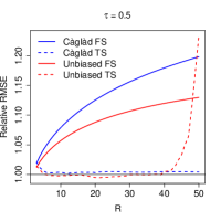
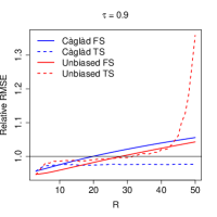
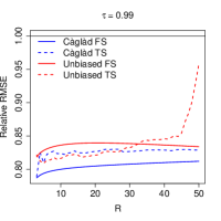
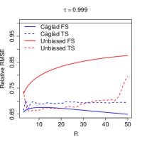
(a) $T=50$

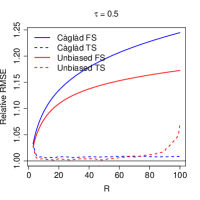
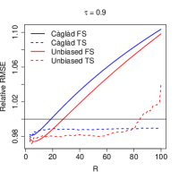
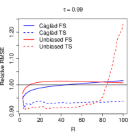
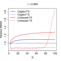
(b) $T=100$

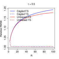
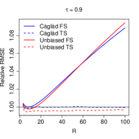
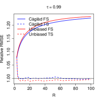
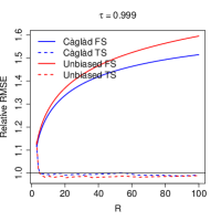
(c) $T=500$

Figure 1. GEV: relative RMSE for different choices of $R$.

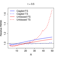
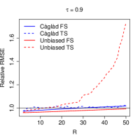
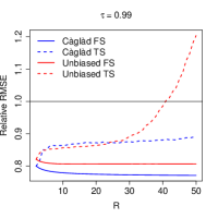
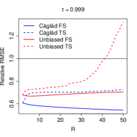
(a) $T=50$

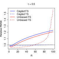
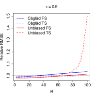
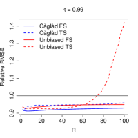
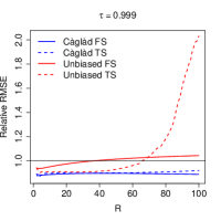
(b) $T=100$

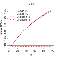
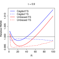
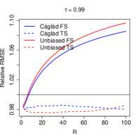
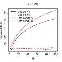
(c) $T=500$

Figure 2. GPD: relative RMSE for different choices of $R$.

5. Choosing the number of L-moments in estimation

The simulation exercise in the previous section evidences that the number of L-moments $R$ plays a crucial role in determining the relative behaviour of the generalised L-moment estimator. In light of this, in this section we introduce (semi)automatic methods to select $R$. We briefly outline two approaches, with the details being left to Supplemental Appendix LABEL:app_selection. We then contrast these approaches in the context of the Monte Carlo exercise of Section 4.

In Supplemental LABEL:higher_order_selector, we derive a higher-order expansion of the “generalised” L-moment estimator (7). We then propose to choose $R$ by minimising the resulting higher-order mean-squared error of a suitable linear combination of the parameters. Similar approaches were considered in the GMM literature by Donald and Newey (2001) – where the goal is to choose the number of instruments in linear instrumental variable models –, and Donald et al. (2009) – where one wishes to choose moment conditions in models defined by conditional moment restrictions (in which case infinitely many restrictions are available). Relatedly, Okui (2009) considers the choice of moments in dynamic panel data models; and, more recently, Abadie et al. (2023) use higher order expansions to develop a method of choosing subsamples in linear instrumental variables models with first-stage heterogeneity. Importantly, our higher-order expansions can be used to provide higher-order mean-squared error estimates of target estimands $g_{T}(\theta_{0})$, where $g_{T}$ is a function indexed by sample size. This can be useful when the parameter $\theta_{0}$ is not of direct interest. So, for example, if our goal is quantile estimation, we can choose $R$ so as to minimise the higher-order mean-squared error of estimating the target quantile.

In Supplemental LABEL:lasso_selector, we consider an alternative approach to selecting L-moments by employing $\ell_{1}$-regularisation. Following Luo et al. (2015), we note that the first order condition of the estimator (7) may be written as:

$$A_{R}h^{R}(\hat{\theta})=0\,,$$

for a $d\times R$ matrix $A_{R}$ which combines the L-moments linearly into $d$ restrictions. The idea is to estimate $A_{R}$ using a Lasso penalty. This approach implicitly performs moment selection, as the method yields exact zeros for several entries of $A_{R}$. In a GMM context, Luo et al. (2015) introduces an easy-to-implement quadratic program for estimating $A_{R}$ with the Lasso regularization. In the Appendix, we show how this algorithm may be extended to our L-moment setting and provide conditions for its validity.

To conclude, we return to the Monte Carlo exercise of Section 4. We contrast the RMSE (relatively to the MLE) of the original L-moment estimator due to Hosking (1990) that sets $R=d$ (FS) with a two-step L-moment estimator where $R$ is chosen so as to minimise a higher-order MSE of the target quantile (TS RMSE), and a “post-lasso” estimator that estimates $\theta_{0}$ using only those L-moments selected by regularised estimation of $A_{R}$ (TS Post-Lasso). For conciseness, we only consider estimators based on the “càglàd” L-moment estimator (3). Additional details on the implementation of each method can be found in Supplemental Appendix LABEL:monte_carlo_select.

Tables 3 and 4 present the results of the different methods in the GEV and GPD exercises. We report in parentheses the average number of L-moments used by each estimator. Overall, the TS RMSE estimator compares favourably to both Hosking’s original estimator and the MLE. In the GEV exercise, the TS RMSE estimator improves upon both the FS estimator and the MLE when $T<500$; and works as well as the MLE and better than FS in the largest sample size. As for the GPD exercise, recall that this is a setting where estimation of the optimal weighting matrix impacts two-step estimators more negatively and where the choice $R=2$ improves upon MLE even in the largest sample size. Consequently, TS RMSE underperforms the FS estimator at most quantiles in sample sizes $T=50$ and $T=100$, and only slightly outperforms it at $T=500$. Note, however, that differences in the GPD setting are mostly small: the average gain of FS over TS RMSE in the GPD exercise is 0.7 (relative) percentage points (pp) and the largest outperformance is 3.9 pp; whereas, in the GEV exercise, the average gain of TS RMSE over FS is 3.3 pp and the largest is 10.8 pp. More importantly, in both settings, our TS RMSE approach is able to simultaneously generate gains over MLE in smaller samples and mitigate inefficiencies of Hosking’s original method in larger sample sizes. This phenomenon is especially pronounced at the tails of the distributions.

With regards to the Post-Lasso method, we note that it behaves similarly to TS RMSE in larger sample sizes, though it can perform unfavourably vis-à-vis the other L-moment alternatives in the smallest sample size (the method still improves upon MLE at tail quantiles in this scenario). As we discuss in Supplemental Appendix LABEL:monte_carlo_select, this issue can be partly attributed to a “harsh” regularisation penalty being used in the selection step. There is room for improving this step by relying on an iterative procedure to select a less harsh penalty (see Belloni et al. (2012) and Luo et al. (2015) for examples). We also discuss in the Appendix that it could be possible to improve the TS RMSE procedure by including additional higher-order terms in the estimated approximate RMSE. We leave exploration of these improvements as future topics of research.

Table 3. GEV : relative RMSE under different selection procedures

	$T=50$				$T=100$				$T=500$
	$\tau=0.5$	$\tau=0.9$	$\tau=0.99$	$\tau=0.999$	$\tau=0.5$	$\tau=0.9$	$\tau=0.99$	$\tau=0.999$	$\tau=0.5$	$\tau=0.9$	$\tau=0.99$	$\tau=0.999$
FS	1.020	0.957	0.787	0.657	1.033	0.982	0.949	0.963	1.031	1.004	1.076	1.114
	(3)	(3)	(3)	(3)	(3)	(3)	(3)	(3)	(3)	(3)	(3)	(3)
TS RMSE	1.003	0.964	0.775	0.635	1.008	0.985	0.921	0.875	1.004	1.000	1.007	1.006
	(16.64)	(3.67)	(3.34)	(3.48)	(32.79)	(3.93)	(3.99)	(4.35)	(20.16)	(35.38)	(41.63)	(44.58)
TS Post-Lasso	1.012	0.975	0.837	0.708	1.016	0.989	0.928	0.877	1.008	1.000	1.009	1.007
	(7.95)	(7.95)	(7.95)	(7.95)	(9.25)	(9.25)	(9.25)	(9.25)	(9.94)	(9.94)	(9.94)	(9.94)

Table 4. GPD : relative RMSE under different selection procedures

	$T=50$				$T=100$				$T=500$
	$\tau=0.5$	$\tau=0.9$	$\tau=0.99$	$\tau=0.999$	$\tau=0.5$	$\tau=0.9$	$\tau=0.99$	$\tau=0.999$	$\tau=0.5$	$\tau=0.9$	$\tau=0.99$	$\tau=0.999$
FS	0.990	0.974	0.800	0.609	0.994	0.990	0.920	0.889	1.004	1.003	0.983	0.977
	(2)	(2)	(2)	(2)	(2)	(2)	(2)	(2)	(2)	(2)	(2)	(2)
TS RMSE	0.964	0.997	0.807	0.631	1.001	0.994	0.959	0.919	0.997	0.998	0.980	0.969
	(2.85)	(4.34)	(2.62)	(2.94)	(73.38)	(5.96)	(99.2)	(99.32)	(99.03)	(98.63)	(99.54)	(99.54)
TS Post-Lasso	0.996	0.995	0.864	0.689	1.000	1.002	0.966	0.956	0.997	1.000	0.987	0.982
	(3.61)	(3.61)	(3.61)	(3.61)	(3.86)	(3.86)	(3.86)	(3.86)	(4.22)	(4.22)	(4.22)	(4.22)

6. Concluding remarks

This paper considered the estimation of parametric models using a “generalised” method of L-moments procedure, which extends the approach introduced in Hosking (1990) whereby a $d$-dimensional parametric model for a distribution function is fit by matching the first $d$ L-moments. We have shown that, by appropriately choosing the number of L-moments and under an appropriate weighting scheme, we are able to construct an estimator that is able to outperform maximum likelihood estimation in small samples from popular distributions, and yet does not suffer from efficiency losses in larger samples. We have developed tools to automatically select the number of L-moments used in estimation, and have shown the usefulness of such approach in Monte Carlo simulations.

The extension of the generalised L-moment approach to semi- and nonparametric settings appears to be an interesting venue of future research. The L-moment approach appears especially well-suited to problems where semi- and nonparametric maximum likelihood estimation is computationally complicated. Alvarez (2022) shows that a semiparametric extension of the generalised L-moment approach is able to produce a computationally attractive and statistically efficient estimator of the semiparametric model proposed by Athey et al. (2021). The study of such extensions in more generality is a topic for future research.

See pages 1- of supplemental.pdf

References

- Abadie et al. (2023) Abadie, A., J. Gu, and S. Shen (2023): “Instrumental variable estimation with first-stage heterogeneity,” Journal of Econometrics.
- Ahidar-Coutrix and Berthet (2016) Ahidar-Coutrix, A. and P. Berthet (2016): “Convergence of Multivariate Quantile Surfaces,” arXiv:1607.02604.
- Alvarez (2022) Alvarez, L. (2022): “Inference in parametric models with many L-moments,” Ph.D. thesis, University of São Paulo.
- Athey et al. (2021) Athey, S., P. J. Bickel, A. Chen, G. W. Imbens, and M. Pollmann (2021): “Semiparametric Estimation of Treatment Effects in Randomized Experiments,” arXiv:2109.02603.
- Barrio et al. (2005) Barrio, E. D., E. Giné, and F. Utzet (2005): “Asymptotics for L2 functionals of the empirical quantile process, with applications to tests of fit based on weighted Wasserstein distances,” Bernoulli, 11, 131 – 189.
- Belloni et al. (2012) Belloni, A., D. Chen, V. Chernozhukov, and C. Hansen (2012): “Sparse Models and Methods for Optimal Instruments With an Application to Eminent Domain,” Econometrica, 80, 2369–2429.
- Billingsley (2012) Billingsley, P. (2012): Probability and Measure, Wiley.
- Boulange et al. (2021) Boulange, J., N. Hanasaki, D. Yamazaki, and Y. Pokhrel (2021): “Role of dams in reducing global flood exposure under climate change,” Nature communications, 12, 1–7.
- Broniatowski and Decurninge (2016) Broniatowski, M. and A. Decurninge (2016): “Estimation for models defined by conditions on their L-moments,” IEEE Transactions on Information Theory, 62, 5181–5198.
- Carrasco and Florens (2014) Carrasco, M. and J.-P. Florens (2014): “On the Asymptotic Efficiency of GMM,” Econometric Theory, 30, 372–406.
- Chernozhukov et al. (2015) Chernozhukov, V., D. Chetverikov, and K. Kato (2015): “Comparison and anti-concentration bounds for maxima of Gaussian random vectors,” Probability Theory and Related Fields, 162, 47–70.
- Crump et al. (2009) Crump, R. K., V. J. Hotz, G. W. Imbens, and O. A. Mitnik (2009): “Dealing with limited overlap in estimation of average treatment effects,” Biometrika, 96, 187–199.
- Csorgo and Revesz (1978) Csorgo, M. and P. Revesz (1978): “Strong Approximations of the Quantile Process,” Annals of Statistics, 6, 882–894.
- Das (2021) Das, S. (2021): “Extreme rainfall estimation at ungauged locations: information that needs to be included in low-lying monsoon climate regions like Bangladesh,” Journal of Hydrology, 601, 126616.
- Dey et al. (2018) Dey, S., J. Mazucheli, and S. Nadarajah (2018): “Kumaraswamy distribution: different methods of estimation,” Computational and Applied Mathematics, 37, 2094–2111.
- Donald et al. (2009) Donald, S. G., G. W. Imbens, and W. K. Newey (2009): “Choosing instrumental variables in conditional moment restriction models,” Journal of Econometrics, 152, 28–36.
- Donald and Newey (2001) Donald, S. G. and W. K. Newey (2001): “Choosing the Number of Instruments,” Econometrica, 69, 1161–1191.
- Fotopoulos and Ahn (1994) Fotopoulos, S. and S. Ahn (1994): “Strong approximation of the quantile processes and its applications under strong mixing properties,” Journal of Multivariate Analysis, 51, 17–45.
- Gourieroux and Jasiak (2008) Gourieroux, C. and J. Jasiak (2008): “Dynamic quantile models,” Journal of Econometrics, 147, 198–205.
- Gupta and Kundu (2001) Gupta, R. D. and D. Kundu (2001): “Generalized exponential distribution: Different method of estimations,” Journal of Statistical Computation and Simulation, 69, 315–337.
- Hansen (1982) Hansen, L. P. (1982): “Large Sample Properties of Generalized Method of Moments Estimators,” Econometrica, 50, 1029–1054.
- Hosking (2007) Hosking, J. R. (2007): “Some theory and practical uses of trimmed L-moments,” Journal of Statistical Planning and Inference, 137, 3024–3039.
- Hosking (1990) Hosking, J. R. M. (1990): “L-Moments: Analysis and Estimation of Distributions Using Linear Combinations of Order Statistics,” Journal of the Royal Statistical Society: Series B (Methodological), 52, 105–124.
- Hosking and Wallis (1987) Hosking, J. R. M. and J. R. Wallis (1987): “Parameter and Quantile Estimation for the Generalized Pareto Distribution,” Technometrics, 29, 339–349.
- Hosking et al. (1985) Hosking, J. R. M., J. R. Wallis, and E. F. Wood (1985): “Estimation of the Generalized Extreme-Value Distribution by the Method of Probability-Weighted Moments,” Technometrics, 27, 251–261.
- Kerstens et al. (2011) Kerstens, K., A. Mounir, and I. V. De Woestyne (2011): “Non-parametric frontier estimates of mutual fund performance using C- and L-moments: Some specification tests,” Journal of Banking and Finance, 35, 1190–1201.
- Koenker and Machado (1999) Koenker, R. and J. A. Machado (1999): “GMM inference when the number of moment conditions is large,” Journal of Econometrics, 93, 327–344.
- Komunjer and Vuong (2010) Komunjer, I. and Q. Vuong (2010): “Semiparametric efficiency bound in time-series models for conditional quantiles,” Econometric Theory, 26, 383–405.
- Kreyszig (1989) Kreyszig, E. (1989): Introductory Functional Analysis with Applications, Wiley.
- Landwehr et al. (1979) Landwehr, J. M., N. C. Matalas, and J. R. Wallis (1979): “Probability weighted moments compared with some traditional techniques in estimating Gumbel Parameters and quantiles,” Water Resources Research, 15, 1055–1064.
- Li et al. (2021) Li, C., F. Zwiers, X. Zhang, G. Li, Y. Sun, and M. Wehner (2021): “Changes in annual extremes of daily temperature and precipitation in CMIP6 models,” Journal of Climate, 34, 3441–3460.
- Luo et al. (2015) Luo, Y. et al. (2015): “High-dimensional econometrics and model selection,” Ph.D. thesis, Massachusetts Institute of Technology.
- Mason (1984) Mason, D. M. (1984): “Weak Convergence of the Weighted Empirical Quantile Process in ,” Annals of Probability, 12, 243–255.
- Neocleous and Portnoy (2008) Neocleous, T. and S. Portnoy (2008): “On monotonicity of regression quantile functions,” Statistics & Probability Letters, 78, 1226–1229.
- Newey (1990) Newey, W. K. (1990): “Semiparametric efficiency bounds,” Journal of Applied Econometrics, 5, 99–135.
- Newey and McFadden (1994) Newey, W. K. and D. McFadden (1994): “Chapter 36 Large sample estimation and hypothesis testing,” in Handbook of Econometrics, Elsevier, vol. 4, 2111 – 2245.
- Newey and Smith (2004) Newey, W. K. and R. J. Smith (2004): “Higher Order Properties of GMM and Generalized Empirical Likelihood Estimators,” Econometrica, 72, 219–255.
- Newey and West (1987) Newey, W. K. and K. D. West (1987): “A Simple, Positive Semi-Definite, Heteroskedasticity and Autocorrelation Consistent Covariance Matrix,” Econometrica, 55, 703–708.
- Okui (2009) Okui, R. (2009): “The optimal choice of moments in dynamic panel data models,” Journal of Econometrics, 151, 1–16.
- Parzen (1960) Parzen, E. (1960): Modern probability theory and its applications, Wiley.
- Portnoy (1991) Portnoy, S. (1991): “Asymptotic behavior of regression quantiles in non-stationary, dependent cases,” Journal of Multivariate Analysis, 38, 100 – 113.
- Rothenberg (1971) Rothenberg, T. J. (1971): “Identification in Parametric Models,” Econometrica, 39, 577–91.
- Sankarasubramanian and Srinivasan (1999) Sankarasubramanian, A. and K. Srinivasan (1999): “Investigation and comparison of sampling properties of L-moments and conventional moments,” Journal of Hydrology, 218, 13–34.
- Šimková (2017) Šimková, T. (2017): “Statistical inference based on L-moments,” Statistika, 97, 44–58.
- Vaart (1998) Vaart, A. W. v. d. (1998): Asymptotic Statistics, Cambridge Series in Statistical and Probabilistic Mathematics, Cambridge University Press.
- Vaart and Wellner (1996) Vaart, A. W. V. d. and J. A. Wellner (1996): Weak convergence and empirical processes, Springer.
- Wang and Hutson (2013) Wang, D. and A. D. Hutson (2013): “Joint confidence region estimation of L-moment ratios with an extension to right censored data,” Journal of Applied Statistics, 40, 368–379.
- Wang (1997) Wang, Q. J. (1997): “LH moments for statistical analysis of extreme events,” Water Resources Research, 33, 2841–2848.
- Wooldridge (2010) Wooldridge, J. (2010): Econometric analysis of cross section and panel data, Cambridge, Mass: MIT Press.
- Yang et al. (2021) Yang, J., Z. Bian, J. Liu, B. Jiang, W. Lu, X. Gao, and H. Song (2021): “No-Reference Quality Assessment for Screen Content Images Using Visual Edge Model and AdaBoosting Neural Network,” IEEE Transactions on Image Processing, 30, 6801–6814.
- Yoshihara (1995) Yoshihara, K. (1995): “The Bahadur representation of sample quantiles for sequences of strongly mixing random variables,” Statistics & Probability Letters, 24, 299 – 304.
- Yu (1996) Yu, H. (1996): “A note on strong approximation for quantile processes of strong mixing sequences,” Statistics & Probability Letters, 30, 1 – 7.
- Zwet (1980) Zwet, W. R. V. (1980): “A Strong Law for Linear Functions of Order Statistics,” Annals of Probability, 8, 986 – 990.