Bayesian Repulsive Mixture Modeling with Matérn Point Processes

Abstract

Mixture models are a standard tool in statistical analysis, widely used for density modeling and model-based clustering. Current approaches typically model the parameters of the mixture components as independent variables. This can result in overlapping or poorly separated clusters when either the number of clusters or the form of the mixture components is misspecified. Such model misspecification can undermine the interpretability and simplicity of these mixture models. To address this problem, we propose a Bayesian mixture model with repulsion between mixture components. The repulsion is induced by a generalized Matérn type-III repulsive point process model, obtained through a dependent sequential thinning scheme on a primary Poisson point process. We derive a novel and efficient Gibbs sampler for posterior inference, and demonstrate the utility of the proposed method on a number of synthetic and real-world problems.

Keywords Poisson process  $\cdot$ Thinning  $\cdot$ Data Augmentation  $\cdot$ Parsimony

1 Introduction

As statistics and machine learning methods find wide application in real world problems, practitioners are increasingly seeking to balance statistical fidelity and predictive accuracy with interpretability, parsimony and fairness. Popular instances of these trade-offs include introducing smoothness, sparsity or low-dimensional structure into statistical models. In this paper, we focus on interpretability and diversity, through the use of repulsive priors in mixture modeling applications. Mixture models are a powerful and flexible class of models, capable of approximating increasingly complex distributions as the number of mixture components increases. Such models are useful both in density modeling applications as well as in clustering applications (McLachlan and Basford, 1988; Banfield and Raftery, 1993; Bensmail et al., 1997), with goals for the latter typically including data exploration, visualization and summarization. Problems where they have been applied include topic modeling (Blei et al., 2003), genetics (Pagel and Meade, 2004; McLachlan et al., 2002) and computer vision (Friedman and Russell, 1997), among many others. However, the flexibility of mixture models often comes at the cost of interpretability and parsimony. For computational tractability, the parameters of the mixture components are typically modeled as independent and identically distributed draws from some ‘base distribution’. This can result in overlapping clusters: unless the clusters are very widely separated, the posterior will typically assign probability to multiple clusters in some neighborhood. The nearly identical locations of these clusters leads to redundancy, and lack of interpretability. Since mixture models are typically composed of simple parametric components, even if the data exhibits clear clustered structure, a slight deviation of individual clusters from the parametric form will again result in overlapping components.

One approach towards addressing this problem is to control the number of mixture components through an appropriate prior. However, trying to induce interpretability in this indirect fashion can make model specification quite challenging, especially in nonparametric applications where the number of components depends on the dataset size. Further, this approach is still sensitive to any misspecification of the form of the individual components. Another approach is to use more flexible (e.g. nonparametric) densities for each component of a mixture model (Gassiat, 2017), though once again this raises problems with model specification, identifiability and computation. A more modern approach is to directly address the problem of overlapping clusters, enforcing diversity through repulsive priors. Here, rather than being sampled independently from the base measure, component locations are jointly sampled from a prior distribution that penalizes realizations where components are situated too close to each other. Such priors typically draw from the point process literature, examples including Gibbs point processes (Stoyan et al., 1987) and determinantal point processes (Hough et al., 2006; Lavancier et al., 2015). Mixture models built on such priors have been shown to provide simpler, clearer and more interpretable results, often without too much loss of predictive performance (Petralia et al., 2012; Xu et al., 2016; Bianchini et al., 2018). Nevertheless, they present computational challenges, since the repulsive models often involve normalization constants that are intractable to evaluate.

In this work, we propose a new class of repulsive priors based on the Matérn type-III point process. Matérn point processes are a class of repulsive point processes first studied in Matérn (1960, 2013). More recently, Rao et al. (2017) developed a simple and efficient Markov chain Monte Carlo (MCMC) sampling algorithm for a generalized Matérn type-III process (see section 2). In this paper, we bring this process to the setting of mixture models, using them as a repulsive prior over the number of components and their locations. Treating the Matérn realization as a latent, rather than a fully observed point process, raises computational challenges that the algorithm from Rao et al. (2017) does not handle. We develop an efficient MCMC sampler for our model and demonstrate the practicality and flexibility of our proposed repulsive mixture model on a variety of datasets. Our proposed algorithm is also useful in Matérn point process applications with missing observations, as well as for mixture models without repulsion, as an alternative to often hard-to-tune reversible jump MCMC methods (Richardson and Green, 1997) to sample the unknown number of components.

We organize this paper as follows. Section 2 reviews the generalized Matérn type-III point process, while section 3 and section 4 outline our proposed Matérn Repulsive Mixture Model (MRMM) and our novel MCMC algorithm. Section 5 discussed related work on repulsive mixture models, and we apply our model to a number of datasets in section 6.

2 Matérn repulsive point processes

The Poisson process (Kingman, 1992) is a completely random point process, where events in disjoint sets are independent of each other. To incorporate repulsion between events, Matérn (1960, 2013) introduced three spatial point process models that build on the Poisson process. The three models, called the Matérn hardcore point process of type I, II and III, only allow point process realizations with pairs of events separated by at least some fixed distance $\eta$, where $\eta$ is a parameter of the model. The three models are constructed by applying different dependent thinning schemes on a primary homogeneous Poisson point process. Despite being theoretically more challenging than the other two processes, the type-III process has the most natural thinning mechanism, and supports higher densities of points.  Rao et al. (2017) showed how this can easily be generalized to include probabilistic thinning and spatial inhomogeneity. Furthermore, Rao et al. (2017) showed that posterior inference for a completely observed type-III process can be carried out in a relatively straightforward manner. These advantages make the generalized Matérn type-III process superior to the other two as a prior for mixture models. For simplicity, we will refer to this process as the Matérn process in the rest of this paper.

Formally, the Matérn process is a finite point process defined on a space ${\Theta}$, parameterized by a thinning kernel ${\mathcal{K}}_{\eta}:{\Theta}\times{\Theta}\to[0,1]$ and a nonnegative intensity function ${\lambda}_{\Theta}:{\Theta}\to[0,\infty)$. We will find it convenient to decompose the function ${\lambda}_{\Theta}(\theta)$ as ${\lambda}_{\Theta}(\theta)={\bar{\lambda}}\cdot p_{\Theta}(\theta)$, for a finite normalizing constant ${\bar{\lambda}}>0$ and some probability density $p_{\Theta}(\theta)$ on $\Theta$. Simulating this process proceeds in four steps: (1) Simulate the primary process ${{F}_{\Theta}}=\left\{{\theta}_{1},\dotsc,{\theta}_{|{{F}_{\Theta}}|}\right\}$ from a Poisson process with intensity ${\lambda}_{\Theta}(\cdot)$ on ${\Theta}$. (2) Assign each event ${\theta}_{j}$ in ${{F}_{\Theta}}$ an independent random birth-time uniformly on the interval ${\mathcal{T}}=[0,1]$. (3) Sequentially visit events in the primary process according to their birth-times (from the oldest to the youngest) and attempt to thin (delete) them. Specifically, at step $j$, the $j$th oldest event $(\theta,t)$ is thinned by each surviving older primary event $(\theta^{\prime},t^{\prime}),t^{\prime}<t$ with probability ${\mathcal{K}}_{\eta}(\theta,\theta^{\prime})$. (4) Write ${{G}_{\Theta}}$ and ${{\tilde{G}}_{\Theta}}$ for the elements of ${{F}_{\Theta}}$ that survive and are thinned from the previous step, respectively. The set ${{G}_{\Theta}}$ forms the Matérn process realization.

For a hardcore Matérn process (figure 1), the thinning kernel satisfies ${\mathcal{K}}_{\eta}\left({\theta},{\theta}_{j}\right)=\mathds{1}_{\|{\theta}-{\theta}_{j}\|<{\eta}}$, where ${\eta}$ is the thinning radius, so that thinning is deterministic: newer events within distance ${\eta}$ of a previously survived event are thinned with probability 1. Other approaches are probabilistic thinning (Rao et al., 2017), where ${\mathcal{K}}_{\eta}\left({\theta},{\theta}_{j}\right)={\eta}_{p}\mathds{1}_{\|{\theta}-{\theta}_{j}\|<{\eta}_{R}}$ (with ${\eta}_{p}\in[0,1]$), or the smoother squared-exponential thinning, where ${\mathcal{K}}_{\eta}\left({\theta},{\theta}_{j}\right)=\exp(-\frac{\|{\theta}-{\theta}_{j}\|^{2}}{2{\eta}})$.  Huber and Wolpert (2009) propose soft-core thinning, where each event ${\theta}_{j}$ has its own thinning radius ${\eta}_{j}$ drawn from some distribution, and ${\mathcal{K}}_{\eta}\left({\theta},{\theta}_{j}\right)=\mathds{1}_{\|{\theta}-{\theta}_{j}\|<{\eta}_{j}}$.

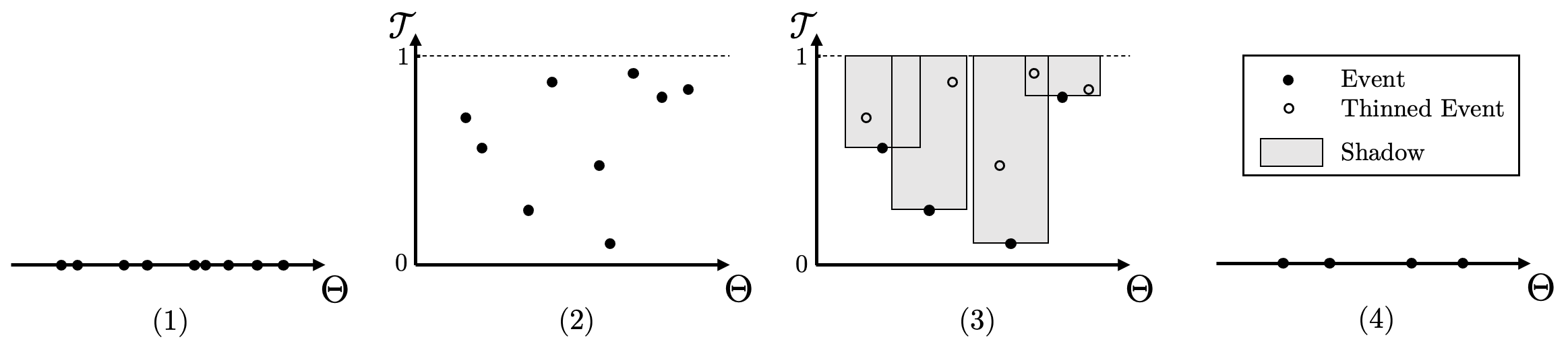
Figure 1: The generative process of a one-dimensional Matérn process with a hardcore thinning kernel ${\mathcal{K}}_{\eta}$. (1) A primary Poisson point process ${{F}_{\Theta}}$ with intensity $\lambda_{\Theta}(\theta)$ is simulated on ${\Theta}$, (2) Events in ${{F}_{\Theta}}$ are assigned random birth times uniformly from ${\mathcal{T}}=[0,1]$, (3) Events in the shadow (i.e. within horizontal distance $\eta$) of earlier surviving events are thinned, (4) Surviving events are projected onto ${\Theta}$ to form the Matérn realization ${{G}_{\Theta}}$.

Observe that since each event ${\theta}_{j}$ has an independently and uniformly distributed birth-time $t_{j}$ associated with it, the set of pairs $\left\{({\theta}_{1},t_{1}),\dotsc,({\theta}_{|{{F}_{\Theta}}|},t_{|{{F}_{\Theta}}|})\right\}$ is itself distributed as a Poisson process on ${\Theta}\times{\mathcal{T}}$, with intensity ${\lambda({\theta},t)}={\lambda}_{\Theta}({\theta})\mathds{1}_{[0,1]}(t)$. We write this extended primary process as ${F}$. Consistent with our use of ${{F}_{\Theta}}$ to represent the set of locations of each point in ${F}$, we will use ${{F}_{\mathcal{T}}}$ to represent the set of birth-times. Similarly, we will use ${G}$ for the extended Matérn events, and ${{G}_{\mathcal{T}}}$ for the associated birth-times (and ${\tilde{G}}$ and ${{\tilde{G}}_{\mathcal{T}}}$ for their thinned counterparts).

Following Rao et al. (2017), we will specify the thinning process through a shadow function $\mathcal{H}_{\eta}:{\Theta}\times{\mathcal{T}}\to[0,1]$ parameterized by a possibly vector-valued ${\eta}$. This gives the probability that an event $({\theta}^{*},{t}^{*})\in{\Theta}\times{\mathcal{T}}$ is thinned by a collection of events ${G}$ as

$${\mathcal{H}_{\eta}\left(({\theta}^{*},{t}^{*}){\,;\,}G\right)} =1-\prod_{{g}\in{G}}\left[1-{\mathcal{H}_{\eta}\left(({\theta}^{*},{t}^{*}){\,;\,}{g}\right)}\right],$$ (1)

where for a single event ${g}=({\theta},{t})$, ${\mathcal{H}_{\eta}\left(({\theta}^{*},{t}^{*}){\,;\,}({\theta},{t})\right)}=\mathds{1}_{[{t},1]}({t}^{*}){\mathcal{K}}_{\eta}\left({\theta}^{*},{\theta}\right)$. Note that the $\mathds{1}_{[t,1]}(t^{*})$ formalizes the fact that an event $({\theta}^{*},{t}^{*})$ can only be thinned by earlier events. We will write $\mathrm{Mat\acute{e}rnThin}_{\mathcal{K}}\left({F},{\eta}\right)$ for the sequential thinning process that assigns elements of ${F}$ to one of ${G}$ or ${\tilde{G}}$ according to thinning kernel ${\mathcal{K}}_{\eta}$ (algorithm 1 in the appendix), and $\text{Proj}_{\mathcal{A}}(\cdot)$ for the operator that projects elements of a set on to some subspace $\mathcal{A}$. The generative process of ${{G}_{\Theta}}\sim\mathrm{Mat\acute{e}rnProcess}_{\mathcal{K}}\left({\lambda},{\eta}\right)$ can be written as

$$\left.{F}\,\middle|\,{\lambda}\right. \sim \mathrm{PoissonProcess}\left({\lambda(\cdot,\cdot)}\right),$$

$$\left.{G},{\tilde{G}}\,\middle|\,{F},{\mathcal{K}}_{\eta}\right. \sim \mathrm{Mat\acute{e}rnThin}_{\mathcal{K}}\left({F},{\eta}\right),\quad{{G}_{\Theta}}=\text{Proj}_{\Theta}({G}).$$

With a Matérn model of point pattern data, one seeks to infer the intensity function ${\lambda}_{\Theta}({\theta})$ and the thinning parameters ${\eta}$ from a realization ${{G}_{\Theta}}$. Observe that for the Matérn type-III process, an event can only be thinned by a surviving event, so that the probability of thinning at any location depends only on the set ${G}$. Rao et al. (2017) showed that in fact, conditioned on ${G}$, the events in ${\tilde{G}}$ are distributed as an inhomogeneous Poisson process with intensity $\lambda_{\Theta}({\theta}){\mathcal{H}_{\eta}\left(({\theta},{t}){\,;\,}G\right)}$. This allowed them to develop an efficient Gibbs sampler when Matérn events ${{G}_{\Theta}}$ are fully observed. This proceeds by sequentially updating the thinned events ${\tilde{G}}$, the Matérn birth times ${{G}_{\mathcal{T}}}$, the Poisson intensity $\lambda_{\Theta}$ and thinning kernel parameter ${\eta}$, each conditioned on the rest. The fact that the thinned events ${\tilde{G}}$ can be jointly sampled avoids the need for any birth-death steps in the MCMC algorithm, both simplifying the algorithm and improving its efficiency. We adapt this sampler for our MCMC algorithm, where the fact that the Matérn events are hidden or partially observed will create new challenges. In the next section, we first describe our model that uses the Matérn process to impose repulsion between components of a finite mixture model.

3 Matérn repulsive mixture model (MRMM)

We start with a primary Poisson process $F$ that includes mixture weights, defining it on an extended space ${\Theta}\times{\mathcal{W}}\times{\mathcal{T}}$ with ${\mathcal{T}}=[0,1],{\mathcal{W}}=[0,\infty)$. Write its intensity function as

$${\lambda({\theta},{w},{t})}={\bar{\lambda}}\cdot{p_{\Theta}\left({\theta}\right)}\cdot{p_{\mathcal{W}}\left({w}\right)}\cdot\mathds{1}_{[0,1]}(t).$$ (2)

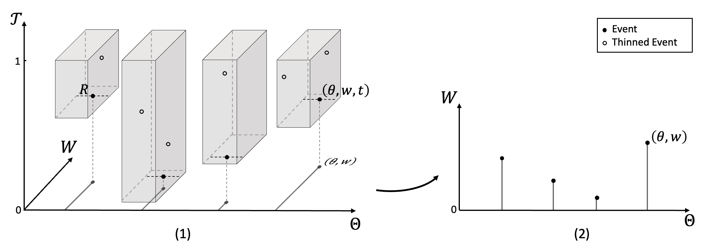
Figure S1: Illustration of the Matérn prior for mixture models. (1) Primary Poisson events ${F}=\left\{({\theta}_{1},{w}_{1},{t}_{1}),\dotsc,({\theta}_{|{F}|},{w}_{|{F}|},{t}_{|{F}|})\right\}$ thinned by a hardcore thinning kernel with thinning radius $R$. The surviving events are projected to the parameter space of the mixture model ${\Theta}\times{\mathcal{W}}$. (2) The resulting mixture model, consisting of a collection of mixture component parameters ${\theta}\in{\Theta}$ and their corresponding unnormalized mixture weights ${w}\in{\mathcal{W}}$.

We will set ${p_{\mathcal{W}}\left({w}\right)}=\mathrm{Gamma}({w}{\,;\,}{\alpha},1)$, while ${p_{\Theta}\left({\theta}\right)}$ will be a problem-specific prior over component parameters. Unlike the Matérn process, we model ${F}$ as a Poisson process conditioned to have at least one event. Given $F$, we will produce a Matérn realization ${G}=\left\{({\theta}_{1},{w}_{1},{t}_{1}),\dotsc,({\theta}_{|G|},{w}_{|G|},{t}_{|G|})\right\}$ by applying $\mathrm{Mat\acute{e}rnThin}_{\mathcal{K}}\left(F,{\eta}\right)$ for some kernel ${\mathcal{K}}$ on $\Theta$ with parameter ${\eta}$. Each element $({\theta},{w},{t})\in G$ will form a component of a mixture model, with ${\theta}$ and ${w}$ representing the parameter and unnormalized weight of that component; see also figure S1 in the appendix. Our model thus serves as a prior over both the number of components in a mixture model, as well as the component weights and locations. Since events in $F$ can only be thinned by surviving events, our modified Matérn prior on $F$ ensures the mixture model has at least one component.

For a set $A$, write $\sum A$ for the sum of its elements. Consistent with the notation of ${{G}_{\Theta}}$ and ${{G}_{\mathcal{T}}}$, we write ${{G}_{\mathcal{W}}}$ for $\text{Proj}_{{\mathcal{W}}}(G)$. Then, given $G$, the observed data ${\bm{X}}=\left\{x_{i},i=1,\dots,n\right\}$ is modeled as follows:

$$\left.x_{i}\,\middle|\,{G}\right.\sim\sum_{({\theta},{w},{t})\in G}\frac{{w}}{\sum{G_{{\mathcal{W}}}}}{p_{\mathcal{X}}\left(\cdot{\,;\,}{\theta}\right)},\quad\quad i=1,\dotsc,n.$$ (3)

Here, ${p_{\mathcal{X}}\left(\cdot{\,;\,}{\theta}\right)}$ represents some family of probability densities parameterized by ${\theta}\in{\Theta}$. As an example, if the observations lie on a Euclidean space, ${p_{\mathcal{X}}\left(\cdot{\,;\,}{\theta}\right)}$ could be a normal distribution, with ${\theta}$ representing the location and variance of a component in a Gaussian mixture model. In this case, the density ${p_{\Theta}\left({\theta}\right)}$ might be a Normal-Inverse-Wishart distribution.

Note that when the $w$’s are independent $\mathrm{Gamma}(\alpha,1)$ variables, the vector of normalized weights $\left({{w}_{1}}\big{/}{\sum{G}_{\mathcal{W}}},\dotsc,{{w}_{|G|}}\big{/}{\sum{G}_{\mathcal{W}}}\right)$ follows a symmetric Dirichlet distribution with concentration parameter $\alpha$ (Devroye, 1986). Thus, conditioned on the number of components, we assume a symmetric Dirichlet prior on the weights. If the thinning kernel ${\mathcal{K}}_{\eta}$ equals $0$, our model then reduces to a standard mixture model, with i.i.d. component parameters, Dirichlet-distributed component weights, and a conditional Poisson distribution on the number of component. Different settings of ${\mathcal{K}}_{\eta}$ (hardcore, probabilistic or squared-exponential thinning) allow different kinds of repulsion between the component parameters. Observe that repulsion is only between the component parameters $\theta$ (and not the component weights $w$). Further, in many settings we allow ${\mathcal{K}}_{\eta}$ to only depend on a subset of the components of $\theta$. For instance, writing ${\theta}=({\theta}^{\mu},{\theta}^{\sigma})$ where ${\theta}^{\mu}$ is the component location and ${\theta}^{\sigma}$ is the component variance, a common requirement is to enforce repulsion only between the component locations, but not their variances. This can easily be achieved by setting ${\mathcal{K}}_{\eta}$ to depend only on ${\theta}^{\mu}$.

All that is left to complete a Bayesian model is to specify hyperpriors on the hyperparameters ${\bar{\lambda}}$ and ${\eta}$, as well as any hyperparameters of the density $p_{\Theta}({\theta})$. The last is problem specific, and is no different from models without repulsion. A natural prior for ${\bar{\lambda}}$ is the Gamma distribution, while the choice of the hyperprior on ${\eta}$ will depend on the type of thinning kernel. In general, we recommend at least a mildly informative prior on the thinning parameter, as otherwise, the posterior can settle on a model without any repulsion. For the hardcore process, where ${\eta}$ is the thinning radius, or for the squared-exponential thinning kernel, where ${\eta}$ is the lengthscale parameter, we can use a Gamma hyperprior. For probabilistic thinning, where ${\eta}=(R,p)$, we can use a Beta prior on the thinning probability $p$, and a Gamma prior on the thinning radius $R$. For this last model, we observe competitive performance even by simply fixing $p=0.95$ and $R$ to a value slightly larger than the desired repulsive distance. We include further discussion of the choice of hyperpriors in section 6 and the appendix.

Write ${\bm{{z}}}=\left({z}_{1},\dotsc,{z}_{n}\right)$ for the collection of latent cluster assignments of the data in equation 3, with ${z}_{i}\in\left\{1,\dots,|G|\right\}$. Following notation in section 2, with hyperpriors omitted for simplicity, the generative process of MRMM is

$$\left.{F}\,\middle|\,{\lambda}\right. \sim\mathrm{PoissonProcess}\left({\lambda(\cdot)}\right)\big{|}{|F|>0},\ \ \quad\qquad\left.{G},{\tilde{G}}\,\middle|\,{F},{\mathcal{K}}_{\eta}\right.\sim\mathrm{Mat\acute{e}rnThin}_{\mathcal{K}}\left({F},{\eta}\right),$$ (4)

$$\left.{z}_{i}\,\middle|\,G\right. \sim\mathrm{Multinomial}\left(\frac{{w}_{1}}{\sum{G}_{\mathcal{W}}},\dotsc,\frac{{w}_{|G|}}{\sum{G}_{\mathcal{W}}}\right),\quad\left.x_{i}\,\middle|\,{z}_{i},G\right.\sim{p_{\mathcal{X}}\left(\cdot{\,;\,}{\theta}_{{z}_{i}}\right)},\qquad i=1,\dotsc,n.$$

Note that for convenience, in the last line above we have imposed an arbitrary ordering on the elements of $G$, and thus the component identities, though the cluster indicators $z_{i}$ really take values in some categorical space. The proposition below gives the joint density of all variables, and will be useful for deriving our posterior sampling algorithm.

Proposition 3.1.

Write $\mathscr{P}_{\lambda}$ for the measure of a rate-$\lambda(\cdot)$ Poisson process on ${{\Theta}\times{\mathcal{W}}\times{\mathcal{T}}}$. Then the measure of the tuple ${\bm{X}}$, ${G}$, ${\tilde{G}}$ has density with respect to $\mathscr{P}_{\lambda}\times{d}x^{n}$ given by

$$p\left({\bm{X}},{G},{\tilde{G}}\,\middle|\,{\lambda},{\eta}\right) =\frac{\mathds{1}(|{G}\cup{\tilde{G}}|>0)}{1-e^{\int_{{{\Theta}\times{\mathcal{W}}\times{\mathcal{T}}}}-\lambda({\theta},{w},{t})\,\mathrm{d}{\theta}\,\mathrm{d}{w}\,\mathrm{d}{t}}}$$

$$\prod_{{g}\in{G}}\left[1-{\mathcal{H}_{\eta}\left({g}{\,;\,}{G}\right)}\right]\prod_{{\tilde{g}}\in{\tilde{G}}}{\mathcal{H}_{\eta}\left({\tilde{g}}{\,;\,}{G}\right)}\prod_{i=1}^{n}\sum_{({\theta},{w},{t})\in{G}}{\frac{{w}}{\sum{G}_{\mathcal{W}}}{p_{\mathcal{X}}\left(x_{i}{\,;\,}{\theta}\right)}}.$$ (5)

4 Posterior inference for MRMM

Given a dataset ${\bm{X}}=\{x_{1},\dotsc,x_{n}\}$ from MRMM, we are interested in the posterior distribution $p\left(G,{\bm{{z}}},{\bar{\lambda}},{\eta}\,\middle|\,{\bm{X}}\right)$, summarizing information about the component weights and locations (through $G$), and the cluster assignments (through ${\bm{{z}}}$). We construct a Markov chain Monte Carlo (MCMC) sampler to simulate from it. Our sampler is an auxiliary variable Gibbs sampler, that for computational reasons, also imputes the thinned events ${\tilde{G}}$. The sampler proceeds by sequentially updating the latent variables ${\bar{\lambda}},{\eta},{G},{\tilde{G}}$ and ${\bm{{z}}}$ according to their conditional posterior distributions. Among these, the most challenging steps are updating ${G}$ and ${\tilde{G}}$: both of these are variable-dimension objects, where not just the values but also the cardinality of the sets must be sampled. Given Matérn events ${G}$, sampling ${\tilde{G}}$ resembles the sampling problem from Rao et al. (2017), where the Matérn realization was completely observed. However, our modified prior on $F$ (where $|F|$ must be greater than $0$) requires some care, and we provide a different and cleaner derivation of this update step using Campbell’s theorem (Kingman, 1992). Updating ${G}$ given the rest is more challenging, and we further augment our MCMC state space with an independent Poisson process ${\tilde{F}}$, and then update the triplet $({G},{\tilde{G}},{\tilde{F}})$ to $({G}^{*},{\tilde{G}}^{*},{\tilde{F}}^{*})$ using a ‘relabeling’ process that keeps the union unchanged. This approach is simpler than reversible-jump or birth-death approaches, with the augmented Poisson intensity trading-off mixing and computation, and forming the only new parameter. Below, we present full details of the Gibbs steps.

1) Updating thinned events ${\tilde{G}}$: Given ${G}$, the thinned events ${\tilde{G}}$ are independent of the observations: $p({\tilde{G}}{\,|\,}{\bar{\lambda}},{\eta},{G},{\bm{{z}}},{\bm{X}})=p({\tilde{G}}{\,|\,}{\bar{\lambda}},{\eta},{G})$. Furthermore, events in ${\tilde{G}}$ can only be thinned by events in ${G}$, suggesting that conditioned on ${G},{\bar{\lambda}},{\eta}$, the events within ${\tilde{G}}$ do not interact with each other, and form a Poisson process. The result below formalizes this:

Proposition 4.1.

Given all other variables, the conditional distribution of the thinned events ${\tilde{G}}$ is a Poisson process with intensity ${{\lambda(\cdot)}{\mathcal{H}_{\eta}\left(\cdot{\,;\,}G\right)}}$.

This result resembles that of Rao et al. (2017), though our derivation in the appendix exploits 3.1 and works with densities with respect to the rate-$\lambda$ Poisson measure, and is simpler and cleaner. Simulating such a Poisson process is straightforward: simulate a Poisson process with intensity ${\lambda}(\cdot)$ on the whole space ${{\Theta}\times{\mathcal{W}}\times{\mathcal{T}}}$, and then keep each event ${\tilde{g}}$ in it with probability ${\mathcal{H}_{\eta}\left({\tilde{g}}{\,;\,}{G}\right)}$ (Lewis and Shedler, 1979). This makes jointly updating the entire set ${\tilde{G}}$ easy and efficient, without any tuning parameters.

2) Updating the Matérn events $G$: This step is significantly more challenging, since unlike the thinned events, the Matérn events interact with each other, and with the clustering structure of the data. Consequently, we cannot simply discard $G$ and sample a new realization. Instead, we produce a dependent update of $G$, through a Markov kernel that targets this conditional distribution.

We first discard the cluster assignments ${\bm{{z}}}$; note these can easily be resampled (see step 3 below). A naive approach is then to make a pass through the elements of ${G}\cup{\tilde{G}}$, reassigning each to either ${G}$ or ${\tilde{G}}$ based on the appropriate conditional. This forms a standard sequence of Gibbs updates, and does not involve any reversible jump or stochastic process simulation. At the end of this pass, we have an updated pair $({G}^{*},{\tilde{G}}^{*})$, with ${G}^{*}$ possibly having different number of elements from ${G}$. While this keeps the union $G\cup{\tilde{G}}$ unchanged, our ability to efficiently update ${\tilde{G}}$ might suggest fast mixing.

In our experiments however, we observed poor mixing, especially with hardcore thinning. The latter setting forbids elements of ${G}^{*}$ from lying within each others’ shadow, and also requires ${\tilde{G}}^{*}$ to lie in the shadow of ${G}^{*}$, making it hard to switch an event from the Matérn set to thinned set, or vice versa. To address this, we begin this step by augmenting our MCMC state-space with an independent rate-${\gamma}{\lambda(\cdot)}$ Poisson process ${\tilde{F}}\subset{{\Theta}\times{\mathcal{W}}\times{\mathcal{T}}}$:

$$\left.{\tilde{F}}\,\middle|\,{\gamma},{\lambda}\right.\sim\mathrm{PoissonProcess}\left({\gamma}{\lambda(\cdot)}\right).$$ (6)

We call ${\gamma}>0$ the augmentation factor, which forms a parameter of our MCMC algorithm. Since ${\tilde{F}}$ is simulated independently of all other variables, the joint distribution of $({G},{\tilde{G}},{\tilde{F}})$ conditioned on all other variables has the conditional distribution of $({G},{\tilde{G}})$ as its marginal. Having simulated ${\tilde{F}}$, we cycle through the elements of ${G}\cup{\tilde{G}}\cup{\tilde{F}}$, sequentially relabeling each event as “survived”, “thinned” or “augmented” to produce a new triplet ${G}^{*}\cup{\tilde{G}}^{*}\cup{\tilde{F}}^{*}$. This relabeling is carried to preserve the joint conditional of ${G}^{*},{\tilde{G}}^{*},{\tilde{F}}^{*}$, so that after discarding ${\tilde{F}}^{*}$, we have updated $({G},{\tilde{G}})$ while maintaining their conditional distribution.

The augmented Poisson process ${\tilde{F}}$ more easily allows events to be introduced into, and removed from ${G}$, especially in the hardcore setting. Each relabeling step is straightforward, and requires computing a 3-component probability. For each $e\in{G}\cup{\tilde{G}}\cup{\tilde{F}}$, write ${{G}^{\backslash e}},{{\tilde{G}}^{\backslash e}}$ and ${{\tilde{F}}^{\backslash e}}$ for the sets resulting from removing $e$ (only one of these will change). Write ${S^{\backslash e}}$ for the sum of the unnormalized mixture weights after removing $e$: ${S^{\backslash e}}=\sum{\text{Proj}_{{\mathcal{W}}}({{G}^{\backslash e}})}$. For an observation $x_{i}\in{\bm{X}}$ and event $g=(\theta,w,t)\in G$, write $l^{g}_{i}={w}{p_{\mathcal{X}}\left(x_{i}{\,;\,}{\theta}\right)}$. Write $L^{\backslash e}_{i}=\sum_{g\in{{G}^{\backslash e}}}l^{g}_{i}$, this is the unnormalized likelihood of observation $i$ with event $e$ taken out, and with its cluster assignment marginalized out. Then, following 3.1, and with $e_{\mathcal{W}}=\text{Proj}_{{\mathcal{W}}}(e)$, the probabilities of “survived”, “thinned” or “augmented” are

$$P(e\in G|-) \propto\prod_{i=1}^{n}\frac{l^{e}_{i}{+L^{\backslash e}_{i}}}{{S^{\backslash e}}{+e_{\mathcal{W}}}}\prod_{{g}\in{{G}^{\backslash e}}{\cup\{e\}}}\left[1-{\mathcal{H}_{\eta}({g}{\,;\,}{{G}^{\backslash e}}{\cup\{e\}})}\right]\prod_{{\tilde{g}}\in{\tilde{G}}}{\mathcal{H}_{\eta}({\tilde{g}}{\,;\,}{{G}^{\backslash e}}{\cup\{e\}})},$$

$$P(e\in{\tilde{G}}|-) \propto\prod_{i=1}^{n}\frac{L^{\backslash e}_{i}}{{S^{\backslash e}}}\prod_{{g}\in{{G}^{\backslash e}}}\left[1-{\mathcal{H}_{\eta}({g}{\,;\,}{{G}^{\backslash e}})}\right]\prod_{{\tilde{g}}\in{{\tilde{G}}^{\backslash e}}{\cup\{e\}}}{\mathcal{H}_{\eta}({\tilde{g}}{\,;\,}{{G}^{\backslash e}})},$$ (7)

$$P(e\in{\tilde{F}}|-) \propto{{\gamma}}\prod_{i=1}^{n}\frac{L^{\backslash e}_{i}}{{S^{\backslash e}}}\prod_{{g}\in{{G}^{\backslash e}}}\left[1-{\mathcal{H}_{\eta}({g}{\,;\,}{{G}^{\backslash e}})}\right]\prod_{{\tilde{g}}\in{{\tilde{G}}^{\backslash e}}}{\mathcal{H}_{\eta}({\tilde{g}}{\,;\,}{{G}^{\backslash e}})}.$$

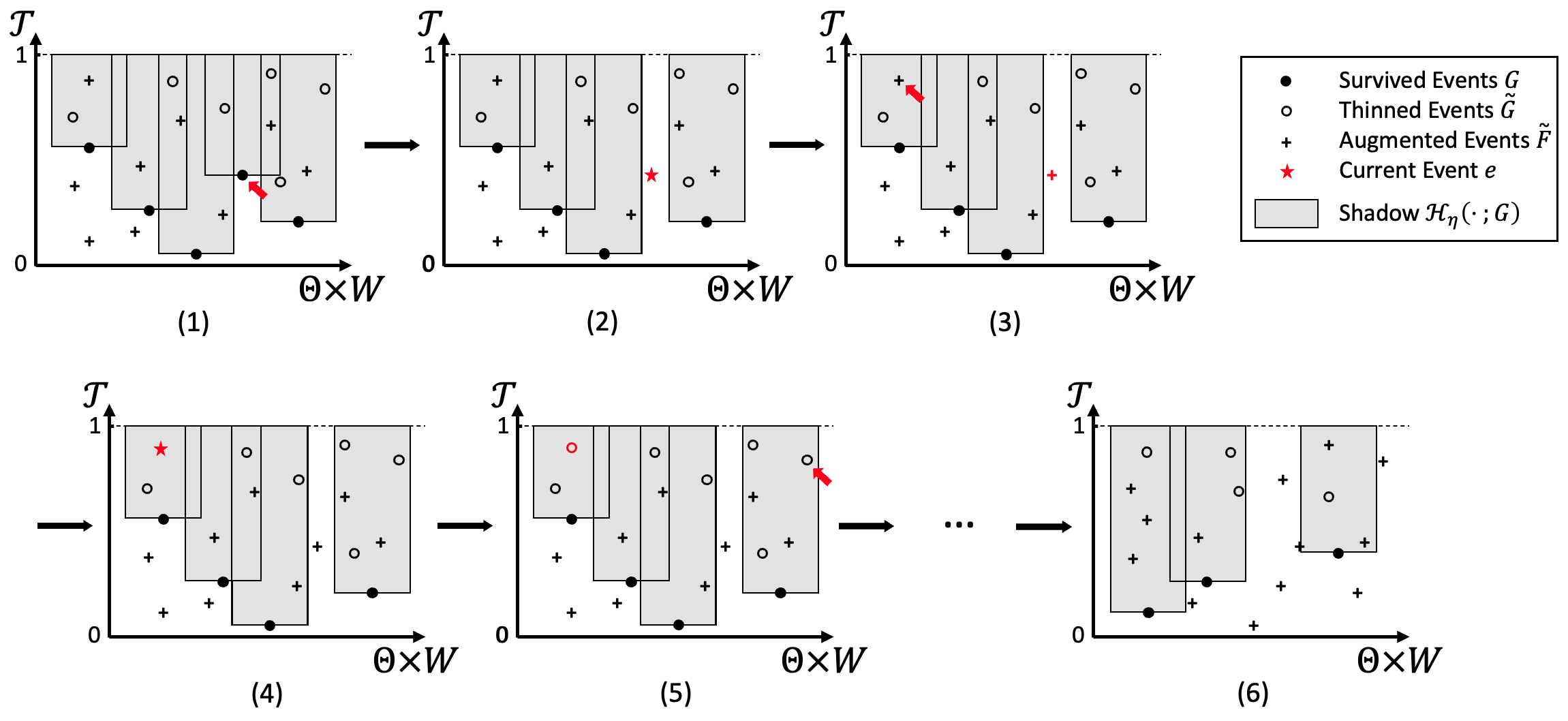
Figure S2: Illustration of the relabeling step. (1) Before relabeling, the state of the surviving events ${G}$, thinned events ${\tilde{G}}$ and auxiliary events ${\tilde{F}}$, and the shadow cast by ${G}$, ${\mathcal{H}_{\eta}\left(\cdot{\,;\,}{G}\right)}$. (2-3) The first event (After random shuffling of all events in ${G}\cup{\tilde{G}}\cup{\tilde{F}}$) is relabeled as “auxiliary”. The event is first removed from its original set ${G}$ (and the shadow is affected accordingly) in (2). Then, in (3), it is relabeled as “auxiliary” according to the posterior conditional probabilities in section 4. Notice that with the hardcore thinning kernel, it is impossible for the event to be relabeled to “thinned”, as it is not under the shadow of a previously surviving event. (4-5) The second event is relabeled as “thinned”. Similarly, the event is removed from the collection of augmented events ${F}$ in (4) and then relabeled as “thinned” in (5). Notice that it is under the shadow of a surviving event, and hence, with the hardcore thinning kernel, it can only be labeled as “thinned” or “auxiliary”. (6) The final state for ${G}$, ${\tilde{G}}$, ${\tilde{F}}$, after all events are relabeled.

Having cycled through all elements of ${G}\cup{\tilde{G}}\cup{\tilde{F}}$, we have a new partition $({G}^{*},{\tilde{G}}^{*},{\tilde{F}}^{*})$, after which the augmented Poisson events ${\tilde{F}}^{*}$ are discarded; see also algorithm 2 and figure S2 in the appendix. The augmented factor ${\gamma}$ in this procedure governs the cardinality of augmented events ${\tilde{F}}$. A larger ${\gamma}$ results in faster mixing, but higher computational cost. Our experiments suggests that a moderate augmentation factor (somewhere between 5 to 10) adequately balances mixing and computation.

3) Updating cluster assignments $z$ and component weights ${{G}_{\mathcal{W}}}$: Given ${\bm{X}}$ and mixture parameters ${{G}_{\Theta}}$ and ${{G}_{\mathcal{W}}}$, we can easily resample the assignments ${\bm{{z}}}$ that were discarded at the start of the previous step. This is no different from standard mixture models; for observation $i$: $p(z_{i}=g|-)\propto l^{g}_{i},\ \forall g\in G.$ Clusters assignments for all observations are conditionally independent, so that these assignments can be carried out in parallel.

In light of the first two update steps, updating the component weights ${{G}_{\mathcal{W}}}$ is not strictly necessary, nevertheless it is very straightforward and improves mixing significantly. Given cluster assignments ${\bm{{z}}}$ and the number of mixture components $|{G}|$, the mixture weights ${{G}_{\mathcal{W}}}=\left\{{w}_{j},j=1,\dots,|{G}|\right\}$ are independent of the other variables. A priori, the ${w}_{j}$’s are independent $\mathrm{Gamma}({\alpha},1)$ random variables, or equivalently, are obtained by multiplying a sample from a $\mathrm{Dirichlet}(\alpha,\dotsc,\alpha)$ distribution (the normalized weights) with an independent sample from a $\mathrm{Gamma}(|G|\alpha,1)$ distribution (the sum of the weights) (Devroye, 1986). We work with the latter representation, and seek to simulate from the posterior distribution of the normalized weights and the sum of the weights. It is easy to see that these continue to be independent under the posterior. The sum of the weights plays no role in the likelihood, and continues to follow a $\mathrm{Gamma}(|G|\alpha,1)$ distribution, while the Dirichlet-multinomial conjugacy implies that the normalized weights follow a $\mathrm{Dirichlet}({\alpha}+n_{1},\dots,{\alpha}+n_{{|{G}|}})$, with $n_{j}$ the number of observations in component $j$.

4) Updating component locations ${{G}_{\Theta}}$ and Matérn birth-times ${{G}_{\mathcal{T}}}$: Again, updating the component locations ${{G}_{\Theta}}$ and birth-times ${{G}_{\mathcal{T}}}$ is not strictly necessary, nevertheless, we find doing it improves mixing. With the number of Matérn events ${G}$ and thinned Matérn events ${G}$ determined, updating these is straightforward, if a little tedious. Unlike standard mixture models, because of repulsion, component locations are not conditionally independent. Write ${\theta}_{j}$ for the location of $j$-th component, and write ${\bm{X}}_{j}$ for the observations assigned to this component. Then, the conditional distribution of ${\theta}_{j}$ is

$$p\left({\theta}_{j}\,\middle|\,{{G}_{\Theta}^{-j}},{{G}_{\mathcal{T}}},{\tilde{G}},{\lambda},{\eta},{\bm{X}}_{j}\right) \propto p\left({G},{\tilde{G}}\,\middle|\,{\lambda},{\eta}\right){p_{\Theta}\left({\theta}_{j}\right)}\prod_{x\in{\bm{X}}_{j}}{p_{\mathcal{X}}\left(x{\,;\,}{\theta}_{j}\right)}.$$ (8)

The term $p({{G},{\tilde{G}}}{\,|\,}{{\lambda},{\eta}})$ accounts for how changing the $j$th event’s location changes the shadow, and therefore the probability of the current Matérn and thinned events. The other two terms are the prior and likelihood of ${\theta}_{j}$ under a mixture model without repulsion. A simple way to simulate from this is with a Metropolis-Hastings step, and when the prior $p_{\theta}$ is conjugate to the likelihood $p(x{\,|\,}{\theta})$, a natural choice for the proposal distribution is the posterior distribution if there were no repulsion: $q_{j}\left({\theta}_{j}\right)\propto{p_{\Theta}\left({\theta}_{j}\right)}\prod_{x\in{\bm{X}}_{j}}{p_{\mathcal{X}}\left(x{\,;\,}{\theta}_{j}\right)}$.

Like the component locations, the birth-times ${{G}_{\mathcal{T}}}$ of the Matérn events can also be updated one at a time. Given the component locations, ${{G}_{\mathcal{T}}}$ is independent of the observations or their cluster assignments, and one only needs to consider their impact on the shadow (3.1). Specifically, if $t_{j}$ is the birth time of the $j$-the event, then

$$p\left({t}_{j}\,\middle|\,-\right)\propto p\big{(}{{G},{\tilde{G}}}\,\big{|}\,{{\lambda},{\eta}}\big{)}\propto\prod_{{g}\in{G}}\big{[}1-{\mathcal{H}_{\eta}\left({g}{\,;\,}{G}\right)}\big{]}\prod_{{\tilde{g}}\in{\tilde{G}}}{\mathcal{H}_{\eta}\left({\tilde{g}}{\,;\,}{G}\right)}.$$

Since $t_{j}\in[0,1]$, simulating from this is straightforward, though it is possible to simplify this further. When the thinning kernel is symmetric, the probability of one event thinning event $j$, were the former the older one, is the same as event $j$ thinning the first if event $j$ were older. Thus, changing $t_{j}$ will only change which could thin which, and not affect the thinning probability. As a result, the first product term does not depend on $t_{j}$, and can be dropped. Next, the birth-times of the thinned events ${\tilde{g}}_{j}=({\tilde{\theta}}_{j},{\tilde{w}}_{j},{\tilde{t}}_{j})\in{\tilde{G}}$ can be used to partition the interval ${\mathcal{T}}=[0,1]$ into segments $[{\tilde{t}}_{j},{\tilde{t}}_{j+1})$, $j=1,\dotsc,{|{\tilde{G}}|}-1$. If the thinning probability is a function only of separation in space (as is the case with all kernels we have considered), then the probability of $t_{j}$ within each segment is constant, depending only on the number of thinned events born before and after the interval $[{\tilde{t}}_{j},{\tilde{t}}_{j+1})$. Specifically, for any time $t$, define ${\tilde{G}}^{\leq t}$ as the subset of events in ${\tilde{G}}$ that were born before or at $t$, and define ${\tilde{G}}^{>t}$ similarly. Then

$$p\left({t}_{j}\in[{\tilde{t}}_{j},{\tilde{t}}_{j+1})\,\middle|\,-\right) \propto\prod_{{\tilde{g}}\in{\tilde{G}}^{\leq t_{j}}}{\mathcal{H}_{\eta}\left({\tilde{g}}{\,;\,}{G^{-j}}\right)}\prod_{{\tilde{g}}\in{\tilde{G}}^{>t_{j}}}{\mathcal{H}_{\eta}\left({\tilde{g}}{\,;\,}{G}\right)}.$$ (9)

Having picked a segment, the exact value of $t_{j}$ is drawn uniformly within the segment.

5) Updating hyperparameters: Hyperparameters include the primary Poisson process intensity, and those in the thinning kernel. The mean intensity ${\bar{\lambda}}$ controls the cardinality of the primary process $F$, and it is easy to show that with a $\mathrm{Gamma}(a,b)$ prior, and with the constraint $|{F}|>0$, the conditional posterior is $p\left({\bar{\lambda}}\,\middle|\,-\right)\propto\frac{1}{1-e^{-{\bar{\lambda}}}}\mathrm{Gamma}({\bar{\lambda}}{\,;\,}a+{|{F}|},b+1)$.

Next, write $\nu$ for any parameters of the normalized Poisson intensity $p_{\Theta}(\theta{\,|\,}\nu)=\lambda_{\Theta}(\theta)/{\bar{\lambda}}$. For a prior $p_{\nu}(\nu)$, the conditional distribution simplifies as $p(\nu{\,|\,}-)\propto p_{\nu}(\nu)\prod_{\theta\in F_{\Theta}}p_{\Theta}(\theta{\,|\,}\nu)$. Finally, writing ${p_{\eta}}$ for the prior for the thinning parameter ${\eta}$, the posterior is $p\left({\eta}\,\middle|\,-\right)\propto{p_{\eta}}({\eta})\prod_{{g}\in{G}}\left[1-{\mathcal{H}_{\eta}\left({g}{\,;\,}{G}\right)}\right]\prod_{{\tilde{g}}\in{\tilde{G}}}{\mathcal{H}_{\eta}\left({\tilde{g}}{\,;\,}{G}\right)}.$ All three distributions above can be updated using any standard MCMC kernel.

5 Related Work

Work on repulsive mixture models dates back to at least Dasgupta (1999). While that work did not propose a new model for repulsion, it demonstrated the importance of separated components for learning mixture models. An early Bayesian mixture model with repulsion was proposed in Petralia et al. (2012). Here, repulsion was induced through a Gibbs point process mechanism: specifically, the prior probability of any configuration of component locations was proportional to the product of individual component probabilities multiplied by a term that penalizes nearby components. The authors there considered two types of penalties, one corresponding to a product of penalty terms for each pair of components, and one depending on the minimum separation between components, before deriving an MCMC sampler, and proving posterior consistency. Xie and Xu (2019) and Quinlan et al. (2018) generalized this model slightly, and also derived posterior rates of convergence. Fúquene et al. (2019) considered a similar approach to Petralia et al. (2012), though they framed their work in the more general setting of non-local priors. Here, given a collection of nested models, parameter configurations in a more complex model that result in an identical density to some configuration in a simpler model are given zero probability. All these works however face computational challenges: the Gibbs interaction term results in intractable normalization constants. This is especially severe when trying to infer parameters of the repulsive penalty, or switch between models with different numbers of components. Our work replaces the Gibbs point process with the Matérn type-III process, though one can use other underdispersed point processes. In Bianchini et al. (2018), the authors use a determinantal point processes (DPP) (Hough et al., 2006; Scardicchio et al., 2009; Lavancier et al., 2015). While mathematically and computationally elegant, DPPs are not as mechanistic as Gibbs-type models, or our thinning mechanism. In our experiments, we compare with the models of Xie and Xu (2019) and Bianchini et al. (2018). Finally, in Beraha et al. (2022), the authors propose an exact MCMC sampler that like ours work side-steps the need for reversible jump MCMC. This auxiliary variable method focuses on a different class of repulsive models, and relies on a perfect simulation algorithm.

We end by nothing that another line of work takes a post-processing approach, deliberately using over-fitted mixtures with a large number of components, and then discarding unoccupied clusters (Frühwirth-Schnatter and Malsiner-Walli, 2019; Saraiva et al., 2020), and merging nearby clusters together (Malsiner-Walli et al., 2016). Unlike model-based approaches like ours, these are a bit ad hoc, making it difficult to coherently calibrate uncertainty, especially in more complicated hierarchical models. We refer the reader to Frühwirth-Schnatter and Malsiner-Walli (2019) for a comprehensive overview of these and related issues.

6 Experiments

In this section we evaluate different settings of our MRMM model and MCMC algorithm, and compare with two other repulsive models: the DPP-based method of Bianchini et al. (2018) and the repulsive Gaussian mixture model of Xie and Xu (2019). We implemented our method as a Python3 package mrmm. An R implementation of the method of Bianchini et al. (2018) was acquired directly from the authors, while a MATLAB implementation of the method of Xie and Xu (2019) was obtained from their supplementary material.

For our model, for all experiments, we placed a $\mathrm{Gamma}(1,1)$ prior on the unnormalized mixture weights ${w}_{j}$, resulting in a flat Dirichlet prior on the mixing proportions. Unless otherwise specified, we placed a $\mathrm{Gamma}(1,0.1)$ prior on the mean intensity of the primary Poisson process, ${\bar{\lambda}}$. We considered three Matérn thinning kernels, the hardcore, probabilistic and squared-exponential kernel (see table S1 in the supplementary material for details). Recall that with zero repulsion, MRMM reduces to an independent mixture model with a prior on the number of components. As stated earlier, it is important to have a relatively informative hyperprior on the parameters of the repulsive kernel, otherwise the model can revert to no repulsion to maximize the data likelihood. Factors influencing this hyperprior can include the strength/range of repulsion, as well as prior belief about the true number of components. While a closed-form expression for the latter is very hard to obtain (Matérn, 2013), prior simulation affords a practical way to calibrate the choice of hyperprior. For the probabilistic thinning kernel, we found it sufficient to fix both the thinning radius and thinning probability based on such knowledge, since its probabilistic nature allows some robustness to excessive repulsion. We can allow a little more flexibility by fixing the thinning probability to a value like $0.95$, while placing a prior on the thinning radius: for most of our experiments, we used a $\mathrm{Gamma}(4,2)$ prior, which had mean 2 and variance 1. We used the same prior on the thinning radius of the hardcore kernel, and on the length-scale in the squared-exponential kernel.

We evaluated model and sampler performance along three dimensions: computational efficiency, goodness-of-fit and parsimony. For computational efficiency, we first computed the effective sample size (ESS) of a number of posterior statistics (for simplicity, we reported only one of them, the number of components, though others like the parameter $\eta$ perform similarly). ESS estimates the number of uncorrelated samples that a sequence of dependent MCMC samples corresponds to, and to compute this, we used the effectiveSize function from the R package coda (Plummer et al., 2006). Dividing this by the total run CPU runtime of the MCMC sampler, we get the ESS per second (ESS/s), an estimate of the cost of producing one independent sample. We use this as our measure of sampler efficiency. We emphasize that since all our models were implemented in different programming languages, this metric should be viewed not as an exact measure of performance, but rather to identify if performances differ by orders of magnitude, and how they scale. To evaluate the goodness-of-fit and predictive accuracy, we reported the predictive likelihood $\ln p\left({\bm{X}}_{\text{test}}\,\middle|\,{\bm{X}}\right)$ of a held-out test dataset ${\bm{X}}_{test}$, as well as the log pseudo-marginal likelihood $\text{LPML}=\sum_{i}\log p\left(x_{i}\,\middle|\,{\bm{X}}^{-i}\right)$ where ${\bm{X}}^{-i}$ denotes the dataset without the $i$-th observation (see Bianchini et al., 2018). To assess the parsimony and interpretability of inferred model, we reported the posterior mean and variance of the number of components ($\mathbb{E}\left[\,{C}\,\middle|\,{\bm{X}}\,\right]$ and $\mathrm{Var}\left({C}\,\middle|\,{\bm{X}}\right)$), as well as a central estimate of the posterior clustering structure (a ‘median’ posterior clustering). The latter was obtained by minimizing the posterior expectation of Binder’s loss function under equal misclassification costs (Bianchini et al., 2018; Lau and Green, 2007). We denote the number of components in this estimate as $\hat{{C}}_{\text{B}}$.

6.1 Effect of augmentation factor ${\gamma}$ on MCMC efficiency

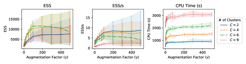
Figure 2: The impact of augmentation factor on (left) MCMC mixing (ESS out of 20,000 iterations), (middle) MCMC mixing rate (ESS/s) and (right) computational cost (CPU time). A tiny perturbation is added to ${\gamma}$’s to ensure visibility.

We focus here on MRMM with hardcore thinning, the most challenging setting for MCMC mixing. We applied MRMM to synthetic data generated from two-dimensional Gaussian mixture models, with minimum component separation of $4.0$ and with varying number of components (see the supplementary material for more details). For each model, we simulated 50 training datasets, each consisting of 20 observations per component. The number of components ${C}$ thus quantifies both model complexity and dataset size. We modeled each dataset as a hardcore MRMM with the thinning radius fixed to 2. The covariance of each component was set to the $2\times 2$ identity matrix $I_{2}$, and the normalized intensity $p_{\Theta}({\theta})$ was set to $N(\mathbf{0},10I_{2})$. For each dataset, we ran our MCMC sampler for 20,000 iterations, with ${\gamma}$ ranging from $1$ to $500$.

Figure 2 plots the raw ESS (left), ESS/s (center) and CPU run-time (right) against the augmentation factor $\gamma$, with each curve representing a different generative model. The right panel shows that, as expected, increasing $\gamma$ results in an increase in CPU time, as the number of events in the augmentation Poisson process increases. At the same time, the leftmost panel shows that this added computational cost comes with the benefit of faster mixing, as more augmented Poisson events more easily allows events to be switched into and out of the Matérn events $G$. For small values for $\gamma$, this improvement is significant, before plateauing out as $\gamma$ crosses $50$. The middle panel shows that this improvement easily compensates for the added computational burden. We see similar results for other thinning kernels, but do not include them. In practice, based on these results, we recommend setting $\gamma$ somewhere in the range of $5$ to $10$. In the rest of our experiments, we fix it to $5$.

6.2 Study of thinning kernels and thinning strengths

Having established that our MCMC sampler mixes well, we now proceed to study the effect of different thinning kernels and thinning strengths on MRMM inferences. Table 1 lists all thinning kernels and corresponding parameters used in this study.

Thinning Kernel	Thinning Parameter		Expression
Hardcore	${\eta}=R$	Radius $R>0$	${{\mathcal{K}}_{R}\left({\theta},{\theta}^{\prime}\right)}=\mathds{1}_{\|{\theta}-{\theta}^{\prime}\|<R}$
Probabilistic	${\eta}=(R,p)$	Radius $R>0$	${{\mathcal{K}}_{(R,p)}\left({\theta},{\theta}^{\prime}\right)}=p\mathds{1}_{\|{\theta}-{\theta}^{\prime}\|<R}$
		Probability $p\in[0,1]$
Squared-exponential	${\eta}=l$	Lengthscale $l>0$	${{\mathcal{K}}_{l}\left({\theta},{\theta}^{\prime}\right)}=\exp\left\{-\frac{\|{\theta}-{\theta}_{j}\|^{2}}{2l}\right\}$

Table 1: Thinning kernels used in experiments

We consider a series of two-dimensional Gaussian mixture models (see figure S5 in the supplementary material). Each model consists of four equally weighted, unit-variance Gaussian components, located at $(-d/2,3d/2)$, $(d/2,d)$, $(d,-d)$, $(-3d/2,-3d/2)$, where $d=1,2,3,4$ quantifies the separation level. A training dataset of size 200 and a test data with 100 observations were simulated independently for each model. We set the prior $p_{\Theta}({\theta})$ to a Gaussian with mean zero and covariance $10I_{2}$, and placed an inverse-Wishart prior with 2 degrees of freedom and a scale matrix $I_{2}$ on the covariances. When learning the thinning strength (thinning radius $R$ for both hardcore and probabilistic MRMM, or the lengthscale $l$ for the squared-exponential MRMM), we placed a $\mathrm{Gamma}(4,2)$ prior with mean 2.0 and variance 1.0. All results were obtained from 2,000 iterations of MRMM after discarding the first 1,000 samples as burn-in.

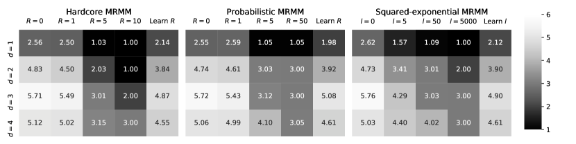
Figure 3: Posterior mean of the number of clusters $\mathbb{E}\left[\,{C}\,\middle|\,{\bm{X}}\,\right]$.

Figure 4: The difference between posterior testing likelihood and the testing likelihood under the ground truth model $M_{0}$, i.e. $\ln p\left({\bm{X}}_{\text{test}}\,\middle|\,{\bm{X}}\right)-\ln p\left({\bm{X}}_{\text{test}}\,\middle|\,M_{0}\right)$.

While the supplementary material discusses the results in detail, we focus here on the heatmaps in figure 4 and figure 4, which, respectively evaluate the parsimony and the goodness-of-fit. As expected, increasing repulsion strength results in greater parsimony, with the posterior mean of the number of clusters dropping. Interestingly, moderate values of repulsion do not significantly harm the model fit. However, a strong repulsion strength does result in a drop in predictive power, especially for the hardcore MRMM. This is a pattern we will continue to see with the real data. In the setting where we learn $R$, we observe good predictive performance, and reasonable parsimony, though a few settings suggest that a stronger prior might be needed.

6.3 Chicago 2019 homocide data

We next consider a dataset of homicide recordings, collected in Chicago, Illinois in the year 2019. This consists 501 entries, and we randomly split these into 416 (85%) training data points and 85 (15%) testing data points. Figure 5 shows the training data, consisting of the latitude and longitude of each homicide, superimposed on a map of Chicago.

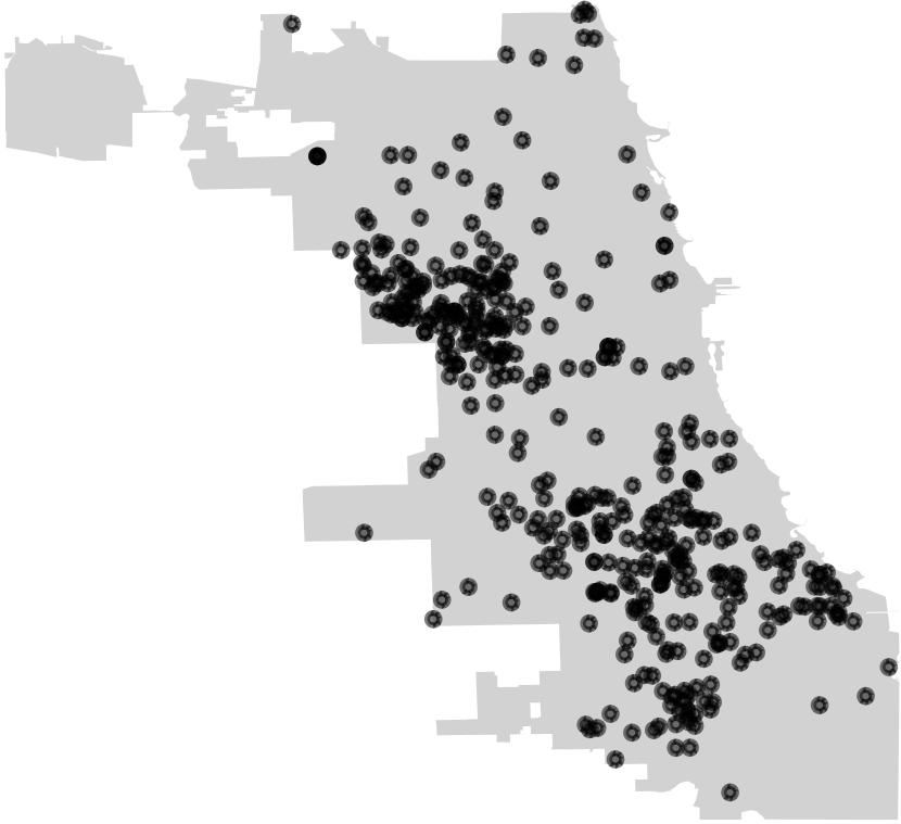
Figure 5: Chicago homicide data.

These range from $(-87.8066,-87.5293)$ to $(41.6572,42.0208)$, and we modeled these with MRMM, specifically, a two-dimensional Gaussian mixture model with hardcore repulsion between component locations. We set $p_{\Theta}({\theta})$ to a Gaussian density, with mean $(-87.6727,41.8180)$ (centered in Chicago), and with variance set to $7\times 10^{-3}I_{2}$ (to cover the entire city). We placed an inverse-Wishart prior with 2 degrees of freedom and scale matrix $3.5\times 10^{-3}I_{2}$ on the covariance of each Gaussian mixture component. In settings where we wished to learn the thinning radius $R$, we placed a $\mathrm{Gamma}(40,200)$ prior on $R$, corresponding to a prior mean of $0.2$ and variance of $0.001$. For all simulations, we ran 5,000 iterations of our MCMC sampler, and discarded the first 2,500 samples as burn-in.

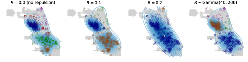
Figure 6: Contours and component assignments of Chicago crime data with hardcore MRMM.

Figure 6 and table 2 show the results from the hardcore MRMM with different thinning radii. Across all posterior samples, there were 3 dominant components, with the remaining components accounting for a small portion of observations. The leftmost panel in figure 6 shows the median clustering without any repulsion: here the observations to the south of Chicago are assigned to three components. Increasing the repulsion radius to $.1$ simplifies these three components into a single large component, even though the observations here deviate slightly from the Gaussian assumption. This is a clear illustration of MRMM being robust to model misspecification. Table 2 shows that this simpler model does not come at the cost of a serious loss in predictive power. Increasing the thinning radius to $.2$ on the other hand causes a steep drop in predictive performance, with a majority of the data points now being assigned to a single component (with a few observations to the north-east assigned to their own component). Inferring the thinning radius results in a posterior mean and variance $\mathbb{E}\left[\,R\,\middle|\,{\bm{X}}\,\right]=0.08$, $\mathrm{Var}\left(R\,\middle|\,{\bm{X}}\right)=0.0001$, and achieves a good trade-off between parsimony and goodness-of-fit. Here again, south Chicago is covered by a single component instead of multiple components as in the no-repulsion case.

Similar results were obtained using probabilistic thinning, we include them in the supplementary material. One takeaway of this and subsequent experiments is that the more complicated probabilistic and softcore thinning mechanisms discussed in Rao et al. (2017) are not necessary in mixture modeling applications. This is largely due to the fact that the number of mixture components is orders of magnitude smaller than the number of observations or events in a point processes. Consequently, the simple hardcore thinning mechanism will typically suffice.

Repulsion strength	$\mathbb{E}\left[\,{C}\,\middle|\,{\bm{X}}\,\right]$	$\mathrm{Var}\left({C}\,\middle|\,{\bm{X}}\right)$	$\hat{{C}}_{\text{B}}$	$\ln p\left({\bm{X}}_{\text{test}}\,\middle|\,{\bm{X}}\right)$	LPML
$R=0.0$ (no repulsion)	5.20	0.4028	5	252.54	1349.08
$R=0.1$	3.51	0.2859	3	248.72	1312.30
$R=0.2$	2.00	0.0000	2	232.95	1223.68
$R\sim\mathrm{Gamma}(40,200)$	3.68	0.2416	4	248.51	1318.73

Table 2: Posterior summaries of hardcore MRMM on Chicago crime dataset.

6.4 Protein structure data

Our next experiment deals with the Malate dehydrogenase protein dataset, publicly available as 7mdh in the protein data bank (Berman et al., 2002). This consists of 500 pairs of torsion angles, each pair $x=(\phi,\psi)\in[-\pi,\pi)\times[-\pi,\pi)$ forming a point on a torus. Figure 7 plots this data, with the right panel showing a planar representation of the data known as the Ramachandran plot (Ramachandran et al., 1963). While the latter shows the underlying clustering structure more clearly, it ignores the fact that the edges wrap back to each other. Consequently, modeling this data with common distributions on two-dimensional Euclidean spaces (e.g. mixture of normals or Betas) is not appropriate. Instead, we model this data as a mixture of uncorrelated bivariate von Mises distributions (Mardia, 1975).

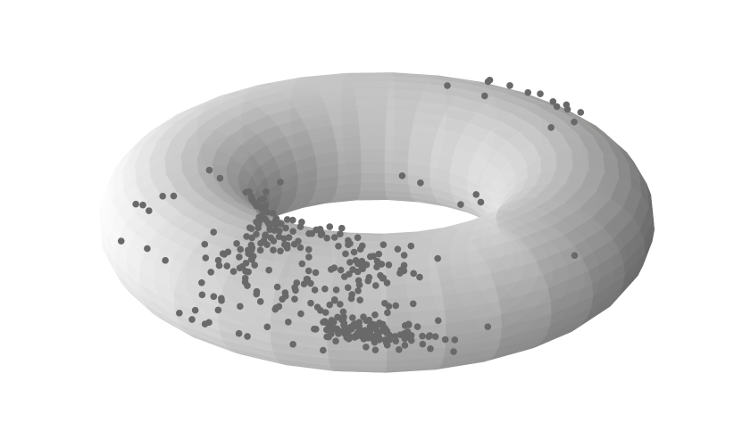
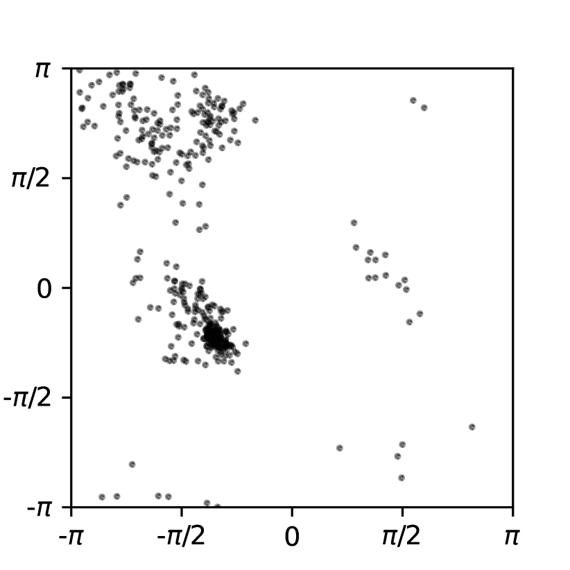
Figure 7: The Malate dehydrogenase protein data, plotted (Left) on a torus. (Right) as a Ramachandran plot, where the torus is flattened to 2-d.

The univariate von Mises distribution is widely used to model one-dimensional angular variables. For $\phi\in[-\pi,\pi)$, its density is $p\left(\phi\,\middle|\,\mu,\kappa\right)=\frac{1}{2\pi I_{0}(\kappa)}\exp\left\{\kappa\cos(\phi-\mu)\right\},$ where $\mu$ is the center of the distribution (mean and mode), $\kappa>0$ measures concentration around this, and the normalization constant $I_{m}(\cdot)$ is the modified Bessel function of the first kind of order $m$. This distribution is analogous to the univariate Gaussian distribution in the Euclidean space, though it captures the periodicity of the angular variables. It converges to the uniform distribution on $[-\pi,\pi)$ when $\kappa\rightarrow 0$. Writing each observation as $x=(\phi,\psi)$, we model these using a Matérn repsulsive mixture model, where under each mixture component, the angles $\phi$ and $\psi$ are independent von Mises variables. Write the parameters of each mixture component as ${\theta}=(\mu_{1},\mu_{2})$ and $\kappa=(\kappa_{1},\kappa_{2})$, then observations from that component have density ${p_{\mathcal{X}}\left(x=(\phi,\psi){\,;\,}{\theta},\kappa\right)}\propto\exp\left\{\kappa_{1}\cos(\phi-\mu_{1})+\kappa_{2}\cos(\psi-\mu_{2})\right\}.$ We set $p_{\Theta}({\theta})$ to the bivariate uniform distribution on $[-\pi.\pi]\times[-\pi,\pi]$, and placed a $\mathrm{Gamma}(10,1)$ prior on the concentration parameter $\kappa$. To induce Matérn thinning, we computed distances on the torus as $d_{2}((\phi,\psi),(\phi^{\prime},\psi^{\prime}))=\sqrt{d_{1}(\phi,\phi^{\prime})^{2}+d_{1}(\psi,\psi^{\prime})^{2}},$ where $d_{1}(\phi,\phi^{\prime})=\min\left\{|\phi-\phi^{\prime}|,\pi-|\phi-\phi^{\prime}|\right\}$. This distance was used in a standard harcore or probabilistic thinning kernel. We note that we can easily extend our model to more sophisticated geodesic distances, or model each component as a bivariate von Mises distribution with correlations (see  Mardia (1975); Mardia et al. (2007)).

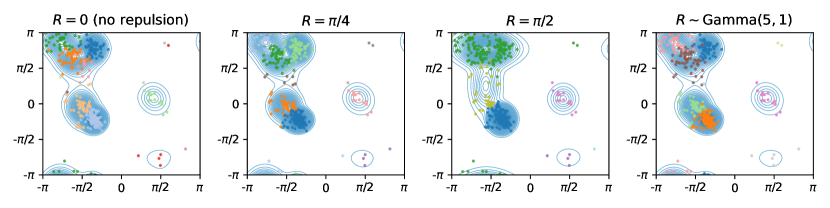
Figure 8: Contours and cluster assignments of the protein data from hardcore MRMM.

Repulsion strength	$\mathbb{E}\left[\,{C}\,\middle|\,{\bm{X}}\,\right]$	$\mathrm{Var}\left({C}\,\middle|\,{\bm{X}}\right)$	$\hat{{C}}_{\text{B}}$	$\ln p\left({\bm{X}}_{\text{test}}\,\middle|\,{\bm{X}}\right)$	LPML
$R=0$ (no repulsion)	12.29	4.1242	14	-177.43	-644.23
$R=\pi/4$	10.22	1.6658	12	-177.52	-646.58
$R=\pi/2$	5.55	0.3999	6	-199.78	-703.62
$R\sim\mathrm{Gamma}(5,1)$	11.13	2.5746	9	-177.76	-647.00

Table 3: Posterior summaries of hardcore MRMM on the Malate protein dataset.

We ran 5,000 MCMC iterations on the hardcore MRMM model and discarded the first half as burn-in. Figure 8 and table 3 show the results with different levels of repulsion. Observe from figure 7 that the data consists three large components of observations, with a couple of smaller components. Our model without repulsion returns about 12 components on average under the posterior distribution, with the leftmost panel of figure 8 showing the median clustering. As with the Euclidean setting, increasing repulsion strength results in fewer components, simpler posterior distributions (indicated by smaller posterior variance) and more interpretable results. A strong repulsion ($R=\pi/2$) produced around 5 components, agreeing with the findings in Mardia et al. (2007), though resulting in a drop in model fit and predictive power. Placing a $\mathrm{Gamma}(5,1)$ prior (mean 5, variance 5) on the thinning radius infers weaker repulsion (a posterior mean and variance for $R$ equal to $0.19\pi$ and $0.017\pi^{2})$, and thus more components ($11$ on average). These results are partly because of our choice of component likelihoods, where the two angles are independent under each component. The component near the origin on the other hand exhibits strong correlation between the angles, and our MRMM model has to split this into two (figure 8, right). As stated earlier, extending our model to allow correlated components is conceptually straightforward using the bivariate von Mises distribution. This however introduces normalization constants for each component that can be quite challenging to compute, requiring techniques from Rao et al. (2016); Lin et al. (2017). To avoid unnecessary complications, we have not followed this path. We emphasize though that modeling repulsion on non-Euclidean spaces using existing models is a less straightforward proposition.

6.5 Comparison with Xie and Xu (2019) on the Old Faithful dataset

The Old Faithful geyser eruption dataset (Silverman, 1986) is a well-known dataset, recording eruption lengths of the Old Faithful geyser in the Yellowstone National Park. In Xie and Xu (2019), the authors evaluated their model on this dataset, and in this section, we use it to compare our model with theirs. Following Xie and Xu (2019), we paired each observed eruption duration time with the time length of the next eruption, resulting in 271 bivariate observations. We split this into training and test sets, with size $219$ and $52$ respectively.

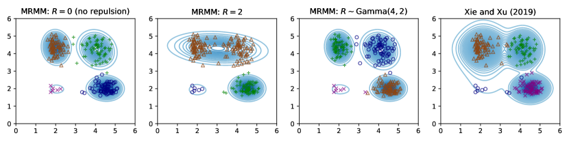
Figure 9: Contours and cluster assignments of Old Faithful dataset with hardcore MRMM.

Consistent with the setup of Xie and Xu (2019), we used a Gaussian distribution for $p_{\Theta}({\theta})$, centered at $(0,0)$, and with covariance $10I_{2}$. For the covariance matrix of each mixture component, Xie and Xu (2019) assumed independence between the two dimensions and placed truncated inverse $\mathrm{Gamma}(1,1)$ priors on the diagonal elements. For MRMM, we used the more natural inverse-Wishart prior with 2 degrees of freedom and scale matrix $I_{2}$ on the covariance matrices. We set the repulsive parameter of Xie and Xu (2019) to its default setting of their code (also the setting in their experiments) below. For different settings of the thinning radius of hardcore MRMM, we ran 5,000 MCMC iterations. Because of issues with MCMC mixing, we had to run the model of Xie and Xu (2019) for 10,000 iterations. For both models, we discarded the first half of the samples as burn-in, and report posterior summaries of both approaches in table 4 and Figure 9.

Model	$\mathbb{E}\left[\,{C}\,\middle|\,{\bm{X}}\,\right]$	$\mathrm{Var}\left({C}\,\middle|\,{\bm{X}}\right)$	$\hat{{C}}_{\text{B}}$	$\ln p\left({\bm{X}}_{\text{test}}\,\middle|\,{\bm{X}}\right)$	LPML	Runtime (s)	ESS/s
Xie and Xu (2019)	3.71	0.2116	4	-104.32	-464.22	225.6	0.01
MRMM:
$\ R=0$	4.02	0.0177	4	-95.80	-421.17	266.5	0.67
$\ R=2$	3.00	0.0000	3	-114.84	-489.83	251.1	5.54
$\ R\sim\mathrm{Gamma}(4,2)$	4.01	0.0119	4	-95.77	-420.54	279.4	0.07

Table 4: Posterior summaries of hardcore MRMM on the Old Faithful geyser eruption data.

First, observe that this dataset consists of four clearly separated components, and for all models, the posterior mean of the number of components was around this value. MRMM returns slightly higher estimates of this quantity compared to Xie and Xu (2019), but with a much smaller sample variance, suggesting that the posterior is simpler and more concentrated. So long as the thinning radius is not forced to too large a value, MRMM also returns much better fits, both in terms of predictive likelihood and LPML. Observe that both the model of Xie and Xu (2019) and MRMM with $R=2$ merge the two top components into a large component, whereas other settings of MRMM keep them clearly separated. In these settings, instead of compromising model fit, MRMM tends to simplify the posterior by concentrating around this solution, and avoiding additional extraneous components. This is also the case with a $\mathrm{Gamma}(4,2)$ prior on $R$, here the thinning radius has posterior mean $\mathbb{E}\left[\,R\,\middle|\,{\bm{X}}\,\right]=1.40$ and variance $\mathrm{Var}\left(R\,\middle|\,{\bm{X}}\right)=0.1864$, with an average of $4$ components.

We also reported the CPU run time to produce 5000 samples in table 4, with both requiring roughly the same time per iteration (note though that Xie and Xu (2019) implemented their approach in Matlab and MRMM was written in Python). As we noted earlier, mixing in their case was poorer, and we had to run their algorithm for twice the number of iterations as ours to get stable results. This can also be seen in the reported ESS/s numbers, where our sampler shows larger (often much larger) values. Results for probabilistic MRMM can be found in the supplementary material.

6.6 Comparison with Bianchini et al. (2018) on the Galaxy dataset

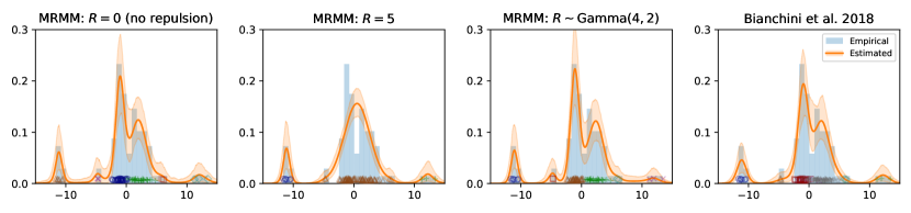
Figure 10: Contour plot and cluster assignments of the Galaxy data for hardcore MRMM.

The Galaxy dataset (Roeder, 1990) is publicly available as part of the DPpackage in R, and contains 82 measured velocities of different galaxies from six well-separated conic sections of space. In Bianchini et al. (2018), the authors evaluated their model on this well-known dataset, using LPML as their goodness-of-fit criteria. We use the same in this section. Following the same preprocessing steps described in Bianchini et al. (2018), we centered the data and rescaled it by a factor of $10^{-3}$, which resulted in a dataset ranged from $-11.65$ to $13.45$. Like Bianchini et al. (2018), we set $p_{\Theta}({\theta})$ to place a mean 0 and standard deviation 10 Gaussian prior on the component locations, and an inverse-$\mathrm{Gamma}(3,3)$ prior on the variance of each mixture component. We ran both samplers for 10,000 iterations, and discarded the first 5,000 iterations as burn-in. Figure 10 and table 5 present the results of MRMM with hardcore thinning, along those of with Bianchini et al. (2018).

Model	$\mathbb{E}\left[\,{C}\,\middle|\,{\bm{X}}\,\right]$	$\mathrm{Var}\left({C}\,\middle|\,{\bm{X}}\right)$	$\hat{{C}}_{\text{B}}$	LPML	Runtime (s)	ESS/s
Bianchini et al. (2018)	6.00	1.2180	7	-207.94	600.4	0.02
MRMM:
$\ R=0$ (no repulsion)	7.69	4.0819	6	-210.13	772.9	0.83
$\ R=5$	3.37	0.3046	3	-212.05	448.2	4.50
$\ R\sim\mathrm{Gamma}(4,2)$	5.51	0.9339	6	-208.83	501.2	0.03

Table 5: Posterior summaries for the Galaxy dataset inferred with hardcore MRMM.

The left-most panel in figure 10 dispays the mean posterior density for the model without any repulsion. For this model, the posterior mean number of components is around 8, with a relatively large variance of 4. The two rightmost panels show the corresponding densities for MRMM (with a Gamma prior on the thinning radius), and the model of Bianchini et al. (2018). Both models have about 6 components, though the posterior density or the predictive performance is not significantly different from the model without repulsion. By forcing the thinning radius to $5$, the components around the origin merge into a single component. Whether this is an appropriate amount of repulsion must be determined by the practitioner, though we note that even here, the drop in performance, while noticeable, is not very large. With a $\mathrm{Gamma}(4,2)$ prior on $R$, we get a posterior mean $\mathbb{E}\left[\,R\,\middle|\,{\bm{X}}\,\right]=1.54$ and variance $\mathrm{Var}\left(R\,\middle|\,{\bm{X}}\right)=0.5305$, with the posterior mean of the number of components about $5.5$. With the caveat that Bianchini et al. (2018) was written in R, and our model in Python, we report the CPU run times and ESS/s of both methods in table 5. These are comparable.

7 Discussion

In this paper, we have described a novel approach to repulsive mixture modeling through the Matérn type-III repulsive point process. We have derived a novel, simple and efficient MCMC sampling algorithm and evaluated the algorithm and model on a number of synthetic and real datasets. There are a number of open avenues for future investigation. Firstly, it is of interest to apply our model to new applications and settings. While we only considered repulsion between component locations, it is also of interest to consider settings when repulsion between variances is of interest. This is relevant when we expect clusters to overlap but still seek to enforce parsimony. Another extension is to introduce Matérn repulsive mechanisms into more general latent variable models such as latent feature models and time series models such as self-avoiding Markov models. Even restricting ourselves to mixture models, problems arise when working with high-dimensional parameter spaces. In general high-dimensional spaces present unique challenges to repulsive mixture models, since with high probability, every event is ‘far away’ from every other. Nevertheless, our Matérn approach offers unique possibilities to deal with these. Possible approaches include projecting down to a lower-dimensional space before carrying out Matérn thinning. From a theoretical viewpoint, to better understand the effect of the Matérn kernel parameters on the number of components, as well as on the repulsive behavior they produce. Theoretically characterising repulsive behavior in this fashion will provide practitioners with an additional tool to guide model selection. It is also of interest to investigate asymptotic consistency of this class of repulsive mixture models, and also quantify rates of posterior convergence. This will follow much along the lines of Xie and Xu (2019), though the specifics of the Matérn repulsion will require some care. It is also of interest to quantify the rate of MCMC mixing, and conditions under which it exhibits desirable properties like geometric ergodicity. Finally, it is of interest to apply these models to new applications and problems.

Acknowledgements: The authors gratefully acknowledge the National Science Foundation for support under grants IIS-1816499 and DMS-1812197.

Supplementary material for
“Bayesian Repulsive Mixture Modeling with
Matérn Point Processes”

These supplementary materials include the detailed proofs, algorithms and additional experiment results.

A Proofs

Proposition (3.1).

Write $\mathscr{P}_{\lambda}$ for the measure of a Poisson process on ${{\Theta}\times{\mathcal{W}}\times{\mathcal{T}}}$ with intensity $\lambda({\theta},{w},{t})$. Then the tuple ${\bm{X}}$, ${G}$, ${\tilde{G}}$ has joint density with respect to $\mathscr{P}_{\lambda}\times{\,\mathrm{d}}x^{n}$ given by

$$p\left({\bm{X}},{G},{\tilde{G}}\,\middle|\,{\lambda},{\eta}\right) =\left(\frac{\mathds{1}(|{G}\cup{\tilde{G}}|>0)}{1-e^{\int_{{{\Theta}\times{\mathcal{W}}\times{\mathcal{T}}}}-\lambda({\theta},{w},{t})\,\,\mathrm{d}{\theta}\,\mathrm{d}{w}\,\mathrm{d}{t}}}\right)$$

$$\left(\prod_{{g}\in{G}}\left[1-{\mathcal{H}_{\eta}\left({g}{\,;\,}{G}\right)}\right]\prod_{{\tilde{g}}\in{\tilde{G}}}{\mathcal{H}_{\eta}\left({\tilde{g}}{\,;\,}{G}\right)}\right)\left(\prod_{i=1}^{n}\sum_{({\theta},{w},{t})\in{G}}{\frac{{w}}{\sum{G}_{\mathcal{W}}}{p_{\mathcal{X}}\left(x_{i}{\,;\,}{\theta}\right)}}\right).$$

Proof.

First note that the set ${F}={G}\cup{\tilde{G}}$ follows a Poisson process with rate $\lambda({\theta},{w},{t})$, conditioned to have at least 1 event. The probability that such a Poisson process produces $1$ or more events is $1-\exp(-\int\lambda(\theta,{w},{t})d\theta d{w}d{t})$. It follows that conditioning on this event, ${F}$ has density with respect to $\mathscr{P}_{\lambda}$ given by the ratio in the first parentheses. Each element $f$ of $F$ is assigned to either ${G}$ or ${\tilde{G}}$, with probability ${1-{\mathcal{H}_{\eta}\left({f}{\,;\,}{G}\right)}}$ or ${\mathcal{H}_{\eta}\left({f}{\,;\,}{G}\right)}$ respectively. This gives the terms in the second parentheses. Finally, the $i$th observation is assigned to cluster $({\theta},{w},{t})\in G$ with probability ${w}/{G}_{\mathcal{W}}$, with its value having density ${p_{\mathcal{X}}\left(x_{i}{\,;\,}{\theta}\right)}$ with respect to $dx$. Marginalizing over cluster assignments, and considering all $n$ observations, we get the final terms. The result then follows easily from Lemma A.1. ∎

To prove 4.1, we start with the following useful (and not new) result:

Lemma A.1.

Consider two Poisson processes on some space $\mathcal{Y}$, with intensities $\lambda(y)$ and $\mu(y)$. Then the former has density with respect to the latter given by

$$\frac{d\mathscr{P}_{\lambda}}{d\mathscr{P}_{\mu}}(M):=p_{\mu}(M|\lambda)=e^{\int_{\mathcal{Y}}\mu(y)-\lambda(y)\,\mathrm{d}y}\prod_{m\in M}\frac{\lambda(m)}{\mu(m)}$$ (10)

Proof.

Consider a function $h:\mathcal{Y}\rightarrow\Re$. For a point process $M$ on $\mathcal{Y}$, we overload notation, and define the linear functional $h(M)=\sum_{m\in M}h(m)$. Write $\mathbb{E}_{\mathscr{M}}[h(M)]$ for the expectation of $h(M)$ when $M$ is distributed as a point process with measure $\mathscr{M}$. Recall that $\mathscr{P}_{\lambda}$ corresponds to a rate-$\lambda(\cdot)$ Poisson process on $\mathcal{Y}$, and $\mathscr{P}_{\mu}$, to a rate-$\mu(\cdot)$ Poisson process.We first note that from Campbell’s theorem [Kingman, 1992], for a rate-$\mu(\cdot)$ Poisson process, we have

$$\mathbb{E}_{\mathscr{P}_{\mu}}[\exp(h(M))]=\mathbb{E}_{\mathscr{P}_{\mu}}\left[\exp\bigg{(}\sum_{m\in M}h(m)\bigg{)}\right]=\exp\left(\int(e^{h(y)}-1)\mu(y)\,\mathrm{d}y\right).$$ (11)

Now write $\mathscr{M}^{\lambda}_{\mu}$ for the probability measure of a point process with density $p_{\mu}(M|\lambda)$ with respect to a rate-$\mu(\cdot)$ Poisson process. Then

$$\mathbb{E}_{\mathscr{M}^{\lambda}_{\mu}}[\exp(h(M))] =\mathbb{E}_{\mathscr{P}_{\mu}}\left[p_{\mu}(M|\lambda)\exp(h(M))\right]$$

$$=\mathbb{E}_{\mathscr{P}_{\mu}}\left[e^{\int_{\mathcal{Y}}\left(\mu(y)-\lambda(y)\right)\,\mathrm{d}y}\left(\prod_{m\in M}\frac{\lambda(m)}{\mu(m)}\right)\exp(h(M))\right]$$

$$=e^{\int_{\mathcal{Y}}\left(\mu(y)-\lambda(y)\right)\,\mathrm{d}y}\ \mathbb{E}_{\mathscr{P}_{\mu}}\left[\exp\sum_{m\in M}\left(h(m)+\log{\lambda(m)}-\log{\mu(m)}\right)\right]$$

$$=\exp\left(\int_{\mathcal{Y}}(e^{h(y)}-1)\lambda(y)\,\mathrm{d}y\right)\quad\text{\ (from~{}\lx@cref{creftype~refnum}{eq:laplace})}$$

$$=\mathbb{E}_{\mathscr{P}_{\lambda}}[\exp(h(M))].$$ (12)

This confirms that $\mathscr{M}^{\lambda}_{\mu}$ equals $\mathscr{P}_{\lambda}$ a.e., proving our result. ∎

Proposition (4.1).

Given all other variables, the conditional distribution of the thinned events ${\tilde{G}}$ is a Poisson process with intensity ${{\lambda(\cdot)}{\mathcal{H}_{\eta}\left(\cdot{\,;\,}G\right)}}$.

Proof.

With respect to a rate-$\lambda(\cdot)$ Poisson process,

$$p({\tilde{G}}|-) \propto p\left({G},{\tilde{G}},{\bm{X}}\,\middle|\,{\lambda},{\eta}\right)$$

$$=\left(\frac{\mathds{1}(|{G}\cup{\tilde{G}}|>0)}{1-e^{\int_{{{\Theta}\times{\mathcal{W}}\times{\mathcal{T}}}}-\lambda({\theta},{w},{t})\,\mathrm{d}{\theta}\,\mathrm{d}{w}\,\mathrm{d}{t}}}\right)\prod_{{g}\in{G}}\left[1-{\mathcal{H}_{\eta}\left({g}{\,;\,}{G}\right)}\right]\prod_{{\tilde{g}}\in{\tilde{G}}}{\mathcal{H}_{\eta}\left({\tilde{g}}{\,;\,}{G}\right)}$$

$$\propto\prod_{{\tilde{g}}\in{\tilde{G}}}{\mathcal{H}_{\eta}\left({\tilde{g}}{\,;\,}{G}\right)}.$$

In the last equation, we dropped all terms that do not depend on ${\tilde{G}}$, and used the fact that since $|G|>0$, $\mathds{1}(|{G}\cup{\tilde{G}}|>0)$. The result now follows from Lemma A.1. ∎

B Additional Figures

C Algorithms

1

2

Function $\mathrm{Mat\acute{e}rnThin}_{\mathcal{K}}\left({F},{\eta}\right)$:

       Input : Extended primary Poisson process ${F}$ and thinning kernel ${\mathcal{K}}_{\eta}$

       Output : Extended Matérn events ${G}$ and thinned events ${\tilde{G}}$

3      

4      Write $\overrightarrow{{F}}=\left({f}_{1},\dotsc,{f}_{|{F}|}\right)$ for ${F}$ sorted in ascending order of birth times (so that $\text{Proj}_{{\mathcal{T}}}({f}_{j})<\text{Proj}_{{\mathcal{T}}}({f}_{j^{\prime}})$ if $j<j^{\prime}$).

5      for $j\leftarrow 1$ to ${|{F}|}$ do

6             Set $({\theta},{t})\leftarrow\left(\text{Proj}_{{\Theta}}({f}_{j}),\text{Proj}_{{\mathcal{T}}}({f}_{j})\right)$

7             Draw $u\sim$ Unif$[0,1]$

8             if $u<{\mathcal{H}_{\eta}\left(({\theta},{t})\;{G}\right)}$ then // Assign ${f}_{j}$ to ${G}$ w.p. ${\mathcal{H}_{\eta}\left(({\theta},{t})\;{G}\right)}$

9                   ${G}\leftarrow{G}\cup{f}_{j}$

10            else

11                   ${\tilde{G}}\leftarrow{\tilde{G}}\cup{f}_{j}$

12            

13      

return ${G}$, ${\tilde{G}}$

Algorithm 1 Details of the function $\mathrm{Mat\acute{e}rnThin}_{\mathcal{K}}\left({F},{\eta}\right)$

1

2

Function Relabel(${\lambda}$, ${\gamma}$, ${G}$, ${\tilde{G}}$, ${\bm{X}}$):

       Input : Primary Poisson intensity ${\lambda}$, augmentation factor ${\gamma}$, current state of the surviving events ${G}$ and the thinned events ${\tilde{G}}$, the data ${\bm{X}}$.

       Output : Updated Matérn events ${G}$ and thinned events ${\tilde{G}}$.

3      

4      Sample augmented ${\tilde{F}}\sim\mathrm{PoissonProcess}\left({\gamma}{\lambda}(\cdot)\right)$

5       Impute non-locational parameters of ${\tilde{G}}$ from the prior (if presents in the model)

6       Obtain shuffled indices $J$ = RandomShuffle($\{1,\dots,|{G}\cup{\tilde{G}}\cup{\tilde{F}}|\}$)

7       Compute likelihood related objects: $n\times|J|$ matrix $L=\left({w}_{j}{p_{\mathcal{X}}\left(x_{i}\;{\theta}_{j}\right)}:i,j\right)$ and $n$-dim vector $\bm{l}=\big{(}\sum_{{g}\in{G}}l_{1}^{g},\dots,\sum_{{g}\in{G}}l_{n}^{g}\big{)}$

8       Compute the normalizing constant ${S}=\sum{G}_{\mathcal{W}}$

9       foreach $j$ in $J$ do

10             if event $j$ in ${G}$ then

11                   if ${|{G}|}=1$ then // $G$ contains only event $j$

12                         next

13                  else

14                         ${S}\leftarrow{S}-{w}_{j}$

15                         $\bm{l}\leftarrow\bm{l}-L_{\cdot j}$

16                  

17            Remove event $j$ from its original event set

18             Assign event $j$ to ${G}$, ${\tilde{G}}$ or ${\tilde{F}}$ with probability $P(e\in{G}|-)$, $P(e\in{\tilde{G}}|-)$ and $P(e\in{\tilde{F}}|-)$ in section 4, respectively,

19            

20      return ${G}$, ${\tilde{G}}$

Algorithm 2 The relabeling step to update Matérn events ${G}$

1

2

Input : Data ${\bm{X}}=\left\{x_{1},\dots,x_{n}\right\}$, number of MCMC iterations $M$, model of cluster components ${p_{\mathcal{X}}\left(\cdot\;{\theta}\right)}$, augmentation factor ${\gamma}$, prior on cluster locations $p_{\theta}$, shape parameter of the Gamma prior on weights ${\alpha}$, shape and rate parameter of the Gamma prior on mean intensity $(a,b)$, and prior on thinning kernel parameter ${p_{\eta}}$.

Output : Posterior samples of mean intensity ${\bar{\lambda}}$, thinning parameter ${\eta}$, Matérn events ${G}_{\Theta}$, ${G}_{\mathcal{T}}$, ${G}_{\mathcal{W}}$, thinned events ${\tilde{G}}$, and cluster assignments ${\bm{{z}}}$.

3

4Initialize ${\bar{\lambda}}\sim\mathrm{Gamma}(a,b)$, ${\eta}\sim{p_{\eta}}$

5 Initialize ${G},{\tilde{G}}\sim\mathrm{Mat\acute{e}rnProcess}_{\mathcal{K}}\left({\lambda},{\mathcal{K}}_{\eta}\right)$

6 Initialize ${\bm{{z}}}$ from $\left.{\bm{{z}}}\,\middle|\,{\bm{X}},{G}\right.$: ${z}_{i}\sim\mathrm{Multinomial}\left({w}_{j}\cdot{p_{\mathcal{X}}\left(X_{i}\;{\theta}_{j}\right)},~{}j=1,\dots,{|{G}|}\right)$

7 for $m\leftarrow 1$ to $M$ do

8       Update ${\bar{\lambda}}$ according to $\frac{1}{1-e^{-{\bar{\lambda}}}}\mathrm{Gamma}(a+{|{F}|},b+1)$ using Metropolis-Hastings

9      Update ${\eta}$ according to $p({{\eta}}{\,|\,}{{G},{\tilde{G}}})$

10       Update ${\tilde{G}}$: (Poisson thinning) simulate from $\mathrm{PoissonProcess}\left({\lambda}\right)$ and discard event ${\tilde{g}}$ with probability $1-{\mathcal{H}_{\eta}\left({\tilde{g}}\;{G}\right)}$

11       Update ${{G}_{\mathcal{T}}}$ one at a time according to equation 9

12       Update ${{G}_{\mathcal{W}}}\leftarrow{S}\cdot{\overline{{G}_{\mathcal{W}}}}$ where ${S}\sim\mathrm{Gamma}({|{G}|}{\alpha},1)$ and ${\overline{{G}_{\mathcal{W}}}}\sim\mathrm{Dirichlet}\left({\alpha}+n_{1},\dots,{\alpha}+n_{|{G}|}\right)$ ($n_{j}=\sum_{i=1}^{n}\mathds{1}({z}_{i}=j))$

13       Update ${{G}_{\Theta}}$ one at a time according to equation 8 using Metropolis-Hastings

14       ${G},{\tilde{G}}\leftarrow$Relabel(${\lambda}$, ${\gamma}$, ${G}$, ${\tilde{G}}$, ${\bm{X}}$)

15       Update ${\bm{{z}}}$ one at a time: ${z}_{i}\sim\mathrm{Multinomial}\left({w}_{j}\cdot{p_{\mathcal{X}}\left(X_{i}\;{\theta}_{j}\right)},j=1,\dotsc,{|{G}|}\right)$

16      

return Posterior MCMC samples of ${\bar{\lambda}}$, ${\eta}$, ${G}$, ${\tilde{G}}$ and ${\bm{{z}}}$

Algorithm 3 Bayesian inference of MRMM

D Additional Experimental Results

Thinning Kernel	Thinning Parameter		Expression
Hardcore	${\eta}=R$	Radius $R>0$	${{\mathcal{K}}_{R}\left({\theta},{\theta}^{\prime}\right)}=\mathds{1}_{\|{\theta}-{\theta}^{\prime}\|<R}$
Probabilistic	${\eta}=(R,p)$	Radius $R>0$	${{\mathcal{K}}_{(R,p)}\left({\theta},{\theta}^{\prime}\right)}=p\mathds{1}_{\|{\theta}-{\theta}^{\prime}\|<R}$
		Probability $p\in[0,1]$
Squared-exponential	${\eta}=l$	Lengthscale $l>0$	${{\mathcal{K}}_{l}\left({\theta},{\theta}^{\prime}\right)}=\exp\left\{-\frac{\|{\theta}-{\theta}_{j}\|^{2}}{2l}\right\}$

Table S1: Thinning kernels used in experiments

D.1 Synthetic experiments

In this section, we evaluate MRMM and the associated MCMC sampling algorithm on a number of synthetic tasks. Section D.1.1 provides more details and additional results on the study of augmentation factor ${\gamma}$ in section 6.1, while section D.1.2 compares different thinning kernels and thinning strengths on the same synthetic datasets.

D.1.1 Additional results for section 6.1

The models to generate the datasets are illustrated in figure S3. Figure S4 visualizes assessments for the mixing of one run.

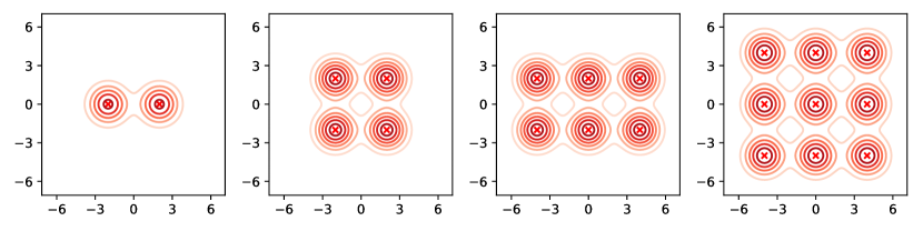
Figure S3: Mixtures of equally weighted Gaussian distributions for the study of augmentation factor ${\gamma}$ in section 6.1. From left to right, number of clusters ${C}=2,4,6,9$, respectively. Each cluster is a standard bivariate Gaussian with covariance being the $2\times 2$ identity matrix $I_{2}$. The minimum distances between cluster centers is 4.

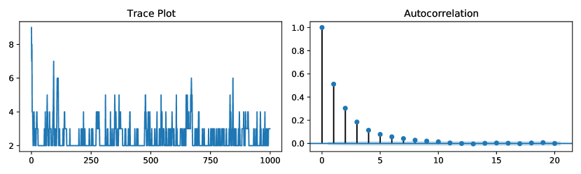
Figure S4: Visualization for assessing mixing of posterior number of clusters ${|{G}|}$ in one run with augmentation factor ${\gamma}=5$ on the dataset with two clusters. In this run, ESS = 5624; ESS/s = 6.97; CPU Time (s) = 806.80. (Left) The trace plot of the first 1,000 updates of ${|{G}|}$. (Right) The autocorrelation function of posterior samples of ${|{G}|}$.

D.1.2 Study of thinning kernels and thinning strengths

Having established that our MCMC sampler mixes well, we now proceed to study the effect of different thinning kernels and thinning strengths on MRMM inferences. Table S1 lists all thinning kernels are corresponding parameters used in this study, specifically, for the probabilistic thinning kernel, the thinning probability $p=0.95$.

We consider a series of two-dimensional Gaussian mixture models shown in figure S5. Each model consists of four equally weighted, unit-variance Gaussian components, located at $(-d/2,3d/2)$, $(d/2,d)$, $(d,-d)$, $(-3d/2,-3d/2)$, where $d=1,2,3,4$ quantifies the separation level. A training dataset of size 200 and a test data with 100 observations were simulated independently for each model.

For MRMM, we set the prior $p_{\Theta}({\theta})$ to a Gaussian with mean zero and covariance $10I_{2}$. We placed an inverse-Wishart prior with 2 degrees of freedom and a scale matrix $I_{2}$ on the covariances. When learning the thinning strength (thinning radius $R$ for both hardcore and probabilistic MRMM, or the lengthscale $l$ for the squared-exponential MRMM), we placed a $\mathrm{Gamma}(4,2)$ prior with mean 2.0 and variance 1.0. All results were obtained from 2,000 iterations of MRMM after discarding the first 1,000 samples as burn-in.

Figure S6, S7 and S8 are the inferred posterior contours and the ‘median’ clustering results obtained with the three kernels. Heatmaps in figures S9, S10, S11, S12 and S13 compare the parsimony and the goodness-of-fit of different thinning kernels with a variety of thinning strengths. As expected, increasing repulsion strength results in greater parsimony, with both the posterior mean and variance of the number of clusters dropping. Interestingly, moderate values of repulsion do not significantly harm the model fit. However, a strong repulsion strength does result in a drop in predictive power, especially for the hardcore MRMM.

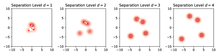
Figure S5: The ground truth model $M_{0}$ with different separation levels.

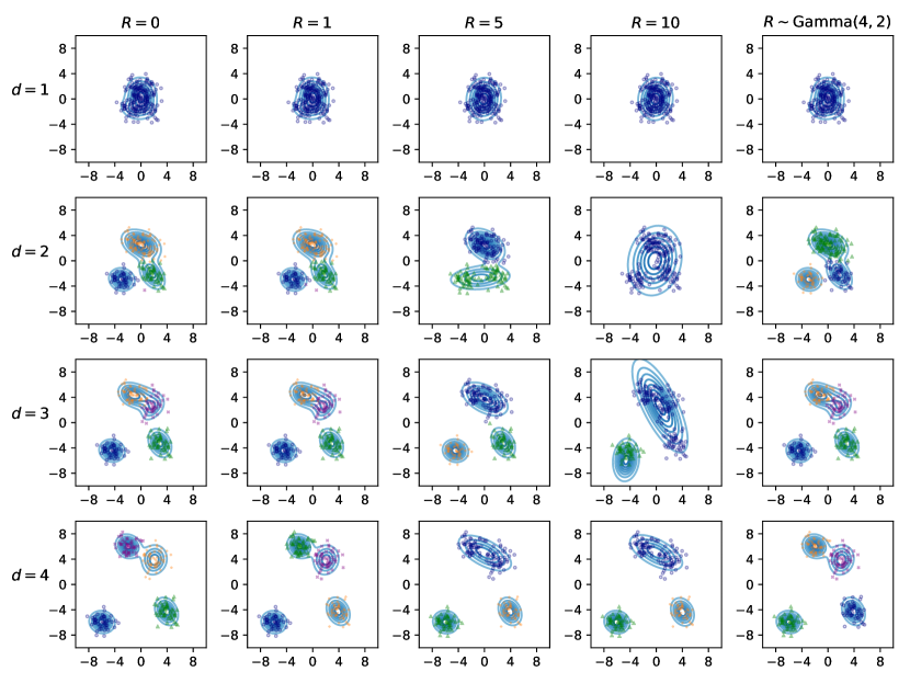
Figure S6: Hardcore MRMM

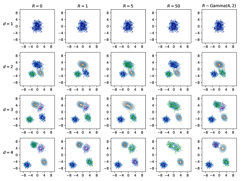
Figure S7: Probabilistic MRMM

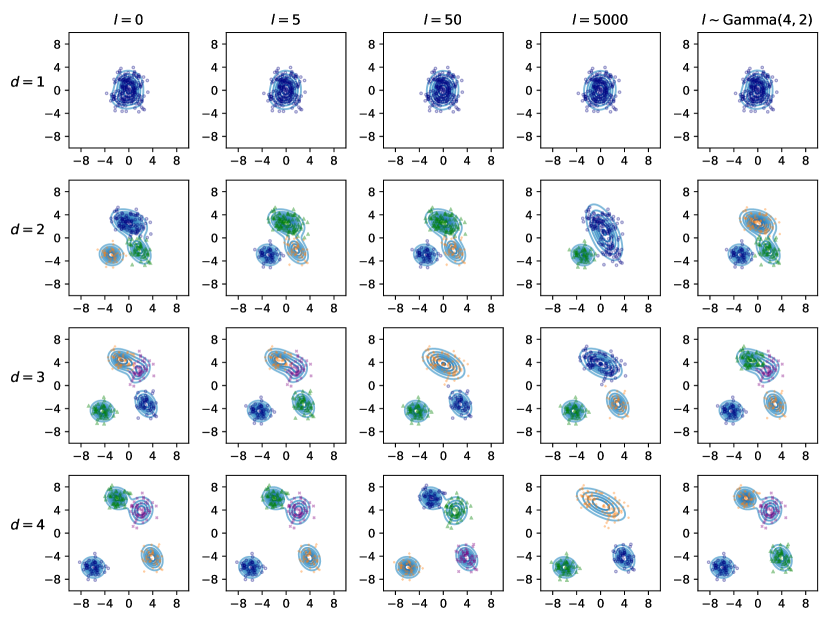
Figure S8: Squared-exponential MRMM

Figure S9: Posterior mean of the number of clusters $\mathbb{E}\left[\,{C}\,\middle|\,{\bm{X}}\,\right]$.

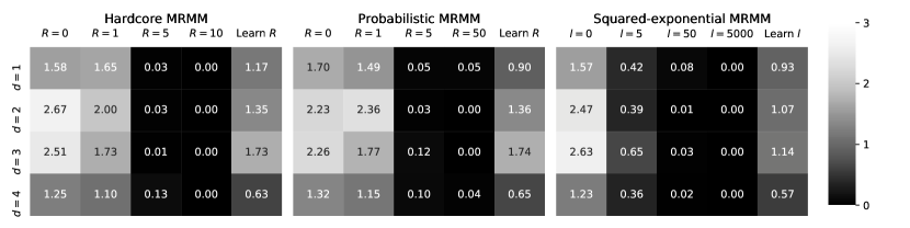
Figure S10: Posterior variance of the number of clusters $\mathrm{Var}\left({C}\,\middle|\,{\bm{X}}\right)$.

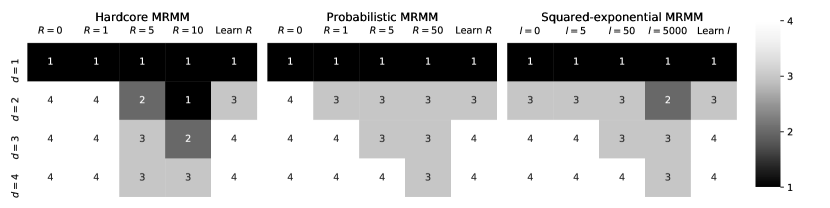
Figure S11: The number of clusters estimated from minimizing the posterior expectation of Binder’s loss function under equal misclassification costs, $\hat{{C}}_{\text{B}}$.

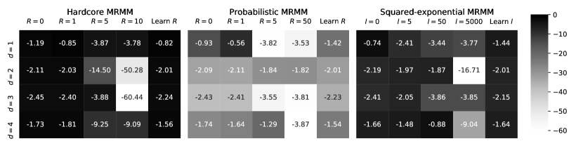
Figure S12: The difference between posterior testing likelihood and the testing likelihood under the ground truth model $M_{0}$, i.e. $\ln p\left({\bm{X}}_{\text{test}}\,\middle|\,{\bm{X}}\right)-\ln p\left({\bm{X}}_{\text{test}}\,\middle|\,M_{0}\right)$.

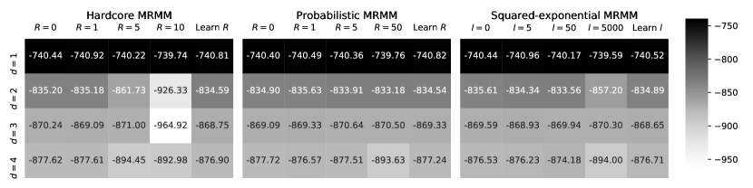
Figure S13: The estimated log pseudo-marginal likelihood (LPML).

D.2 Probabilistic MRMM on real datasets

In this section, we report probabilistic MRMM results on real datasets. The model and parameter settings are the same with the hardcore MRMM reported in the paper, except for the thinning probability, which is fixed to 0.95 in all experiments below.

Chicago 2019 homicide data

Results are shown in figure S14 and table S2.

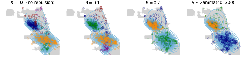
Figure S14: Contour plot and clustering of Chicago crime data from probabilistic MRMM.

Repulsion strength	$\mathbb{E}\left[\,{C}\,\middle|\,{\bm{X}}\,\right]$	$\mathrm{Var}\left({C}\,\middle|\,{\bm{X}}\right)$	$\hat{{C}}_{\text{B}}$	$\ln p\left({\bm{X}}_{\text{test}}\,\middle|\,{\bm{X}}\right)$	LPML
$R=0.0$ (no repulsion)	5.26	0.3914	6	252.20	1351.28
$R=0.1$	4.39	0.2703	5	251.21	1341.60
$R=0.2$	3.00	0.0000	3	247.43	1321.11
$R\sim\mathrm{Gamma}(40,200)$	3.00	0.0040	3	246.73	1324.53

Table S2: Posterior summaries of probabilistic MRMM on Chicago crime dataset. Inferring the thinning radius yields the posterior mean and variance $\mathbb{E}\left[\,R\,\middle|\,{\bm{X}}\,\right]=0.15$, $\mathrm{Var}\left(R\,\middle|\,{\bm{X}}\right)=0.0001$.

Protein structural data

Results are shown in figure S15 and table S3.

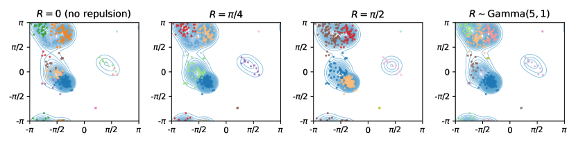
Figure S15: Contour plot and clustering of the protein data from probabilistic MRMM.

Repulsion strength	$\mathbb{E}\left[\,{C}\,\middle|\,{\bm{X}}\,\right]$	$\mathrm{Var}\left({C}\,\middle|\,{\bm{X}}\right)$	$\hat{{C}}_{\text{B}}$	$\ln p\left({\bm{X}}_{\text{test}}\,\middle|\,{\bm{X}}\right)$	LPML
$R=0$ (no repulsion)	12.15	3.5369	13	-142.15	-610.94
$R=\pi/4$	10.14	1.5298	9	-142.36	-618.13
$R=\pi/2$	7.37	0.4056	7	-145.14	-625.13
$R\sim\mathrm{Gamma}(5,1)$	10.85	1.9969	11	-143.64	-622.55

Table S3: Posterior summaries of probabilistic MRMM on the protein dataset. Inferring the thinning radius yields the posterior mean and variance $\mathbb{E}\left[\,R\,\middle|\,{\bm{X}}\,\right]=0.18\pi$, $\mathrm{Var}\left(R\,\middle|\,{\bm{X}}\right)=0.0017\pi^{2}$.

Comparison with Xie and Xu [2019] on the Old Faithful dataset

Results are shown in figure S16 and table S4.

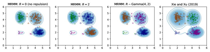
Figure S16: Contour plot and clustering of the Old Faithful geyser eruption data from probabilistic MRMM.

Model	$\mathbb{E}\left[\,{C}\,\middle|\,{\bm{X}}\,\right]$	$\mathrm{Var}\left({C}\,\middle|\,{\bm{X}}\right)$	$\hat{{C}}_{\text{B}}$	$\ln p\left({\bm{X}}_{\text{test}}\,\middle|\,{\bm{X}}\right)$	LPML	Runtime(s)	ESS/s
Xie and Xu [2019]	3.71	0.2116	4	-104.32	-464.22	225.6	0.01
MRMM
$R=0$ (no repulsion)	4.02	0.0157	4	-95.83	-420.53	257.8	14.31
$R=2$	4.00	0.0000	4	-95.93	-419.85	297.6	0.38
$R\sim\mathrm{Gamma}(4,2)$	4.01	0.0138	4	-95.96	-420.94	287.0	2.66

Table S4: Posterior summaries of probabilistic MRMM on the Old Faithful geyser eruption data. Inferring the thinning radius yields the posterior mean and variance $\mathbb{E}\left[\,R\,\middle|\,{\bm{X}}\,\right]=1.39$, $\mathrm{Var}\left(R\,\middle|\,{\bm{X}}\right)=0.1540$.

Comparison with Bianchini et al. [2018] on the Galaxy dataset

Results are shown in figure S17 and table S5.

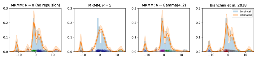
Figure S17: Contour plot and clustering of the Galaxy data from probabilistic MRMM.

Model	$\mathbb{E}\left[\,{C}\,\middle|\,{\bm{X}}\,\right]$	$\mathrm{Var}\left({C}\,\middle|\,{\bm{X}}\right)$	$\hat{{C}}_{\text{B}}$	LPML	Runtime (s)	ESS/s
Bianchini et al. [2018]	6.00	1.2180	7	-207.94	600.4	0.02
MRMM:
$R=0$ (no repulsion)	7.53	4.2370	6	-209.66	734.4	46.9
$R=5$	3.47	0.3772	3	-212.36	410.4	172.4
$R\sim\mathrm{Gamma}(4,2)$	6.23	1.8120	6	-209.43	498.2	13.0

Table S5: Posterior summaries of probabilistic MRMM on the Old Faithful geyser eruption data. Inferring the thinning radius yields the posterior mean and variance $\mathbb{E}\left[\,R\,\middle|\,{\bm{X}}\,\right]=1.87$, $\mathrm{Var}\left(R\,\middle|\,{\bm{X}}\right)=0.3228$.

References

- McLachlan and Basford [1988] Geoffrey J McLachlan and Kaye E Basford. Mixture Models: Inference and Applications to Clustering, volume 38. M. Dekker New York, 1988.
- Banfield and Raftery [1993] Jeffrey D. Banfield and Adrian E. Raftery. Model-based Gaussian and non-Gaussian clustering. Biometrics, pages 803–821, 1993.
- Bensmail et al. [1997] Halima Bensmail, Gilles Celeux, Adrian E Raftery, and Christian P Robert. Inference in model-based cluster analysis. Statistics and Computing, 7(1):1–10, 1997.
- Blei et al. [2003] David M Blei, Andrew Y Ng, and Michael I Jordan. Latent Dirichlet allocation. Journal of Machine Learning Research, 3(Jan):993–1022, 2003.
- Pagel and Meade [2004] Mark Pagel and Andrew Meade. A phylogenetic mixture model for detecting pattern-heterogeneity in gene sequence or character-state data. Systematic Biology, 53(4):571–581, 2004.
- McLachlan et al. [2002] Geoffrey J. McLachlan, Richard W Bean, and David Peel. A mixture model-based approach to the clustering of microarray expression data. Bioinformatics, 18(3):413–422, 2002.
- Friedman and Russell [1997] Nir Friedman and Stuart Russell. Image segmentation in video sequences: a probabilistic approach. In Proceedings of the Thirteenth Conference on Uncertainty in Artificial Intelligence, UAI’97, page 175–181, 1997. ISBN 1558604855.
- Gassiat [2017] Elisabeth Gassiat. Mixtures of nonparametric components and hidden Markov models. Handbook of Mixture Analysis, pages 343–360, 2017.
- Stoyan et al. [1987] Dietrich Stoyan, Wilfrid S Kendall, and Joseph Mecke. Stochastic Geometry and its Applications. John Wiley & Sons, 1987.
- Hough et al. [2006] J Ben Hough, Manjunath Krishnapur, Yuval Peres, Bálint Virág, et al. Determinantal processes and independence. Probability surveys, 3:206–229, 2006.
- Lavancier et al. [2015] Frédéric Lavancier, Jesper Møller, and Ege Rubak. Determinantal point process models and statistical inference. Journal of the Royal Statistical Society - Series B, pages 853–877, 2015.
- Petralia et al. [2012] Francesca Petralia, Vinayak Rao, and David B Dunson. Repulsive mixtures. In Advances in Neural Information Processing Systems, pages 1889–1897, 2012.
- Xu et al. [2016] Yanxun Xu, Peter Müller, and Donatello Telesca. Bayesian inference for latent biologic structure with determinantal point processes (dpp). Biometrics, 72(3):955–964, 2016.
- Bianchini et al. [2018] Ilaria Bianchini, Alessandra Guglielmi, Fernando A Quintana, et al. Determinantal point process mixtures via spectral density approach. Bayesian Analysis, 2018.
- Matérn [1960] Bertil Matérn. Spatial variation: stochastic models and their application to some problems in forest surveys and other sampling investigations. Meddelanden fran statens Skogsforskningsinstitut, 49:144, 1960.
- Matérn [2013] Bertil Matérn. Spatial variation, volume 36. Springer Science & Business Media, 2013.
- Rao et al. [2017] Vinayak Rao, Ryan P Adams, and David D Dunson. Bayesian inference for Matérn repulsive processes. Journal of the Royal Statistical Society - Series B, 79(3):877–897, 2017.
- Richardson and Green [1997] Sylvia Richardson and Peter J Green. On Bayesian analysis of mixtures with an unknown number of components (with discussion). Journal of the Royal Statistical Society - Series B, 59(4):731–792, 1997.
- Kingman [1992] J.F.C. Kingman. Poisson Processes. Oxford Studies in Probability. Clarendon Press, 1992. ISBN 9780191591242.
- Huber and Wolpert [2009] Mark L Huber and Robert L Wolpert. Likelihood-based inference for Matérn type-III repulsive point processes. Advances in Applied Probability, 41(4):958–977, 2009.
- Devroye [1986] Luc Devroye. Non-uniform random variate generation, 1986.
- Lewis and Shedler [1979] PA W Lewis and Gerald S Shedler. Simulation of nonhomogeneous Poisson processes by thinning. Naval Research Logistics Quarterly, 26(3):403–413, 1979.
- Dasgupta [1999] Sanjoy Dasgupta. Learning mixtures of Gaussians. In 40th Annual Symposium on Foundations of Computer Science (Cat. No. 99CB37039), pages 634–644. IEEE, 1999.
- Xie and Xu [2019] Fangzheng Xie and Yanxun Xu. Bayesian repulsive Gaussian mixture model. Journal of the American Statistical Association, pages 1–29, 2019.
- Quinlan et al. [2018] José J Quinlan, Garritt L Page, and Fernando A Quintana. Density regression using repulsive distributions. Journal of Statistical Computation and Simulation, 88(15):2931–2947, 2018.
- Fúquene et al. [2019] Jairo Fúquene, Mark Steel, and David Rossell. On choosing mixture components via non-local priors. Journal of the Royal Statistical Society: Series B (Statistical Methodology), 81(5):809–837, 2019.
- Scardicchio et al. [2009] Antonello Scardicchio, Chase E Zachary, and Salvatore Torquato. Statistical properties of determinantal point processes in high-dimensional Euclidean spaces. Physical Review E, 79(4):041108, 2009.
- Beraha et al. [2022] Mario Beraha, Raffaele Argiento, Jesper Møller, and Alessandra Guglielmi. Mcmc computations for bayesian mixture models using repulsive point processes. Journal of Computational and Graphical Statistics, pages 1–14, 2022.
- Frühwirth-Schnatter and Malsiner-Walli [2019] Sylvia Frühwirth-Schnatter and Gertraud Malsiner-Walli. From here to infinity: sparse finite versus Dirichlet process mixtures in model-based clustering. Advances in Data Analysis and Classification, 13(1):33–64, 2019.
- Saraiva et al. [2020] Erlandson F Saraiva, Adriano K Suzuki, Luís A Milan, et al. A Bayesian sparse finite mixture model for clustering data from a heterogeneous population. Brazilian Journal of Probability and Statistics, 34(2):323–344, 2020.
- Malsiner-Walli et al. [2016] Gertraud Malsiner-Walli, Sylvia Frühwirth-Schnatter, and Bettina Grün. Model-based clustering based on sparse finite Gaussian mixtures. Statistics and computing, 26(1-2):303–324, 2016.
- Plummer et al. [2006] Martyn Plummer, Nicky Best, Kate Cowles, and Karen Vines. CODA: convergence diagnosis and output analysis for MCMC. R News, 6(1):7–11, 2006.
- Lau and Green [2007] John W Lau and Peter J Green. Bayesian model-based clustering procedures. Journal of Computational and Graphical Statistics, 16(3):526–558, 2007.
- Berman et al. [2002] Helen M Berman, Tammy Battistuz, Talapady N Bhat, Wolfgang F Bluhm, Philip E Bourne, Kyle Burkhardt, Zukang Feng, Gary L Gilliland, Lisa Iype, Shri Jain, et al. The protein data bank. Acta Crystallographica Section D: Biological Crystallography, 58(6):899–907, 2002.
- Ramachandran et al. [1963] G. N. Ramachandran, C. Ramakrishnan, and V. Sasisekharan. Stereochemistry of polypeptide chain configurations. J. mol. Biol, 7:95–99, 1963.
- Mardia [1975] K. V. Mardia. Statistical of directional data (with discussion). Journal of the Royal Statistical Society, 37(3):390, 1975.
- Mardia et al. [2007] Kanti V Mardia, Charles C Taylor, and Ganesh K Subramaniam. Protein bioinformatics and mixtures of bivariate von Mises distributions for angular data. Biometrics, 63(2):505–512, 2007.
- Rao et al. [2016] Vinayak Rao, Lizhen Lin, and David B Dunson. Data augmentation for models based on rejection sampling. Biometrika, 103(2):319–335, 2016.
- Lin et al. [2017] Lizhen Lin, Vinayak Rao, and David B Dunson. Bayesian nonparametric inference on the Stiefel manifold. Statistica Sinica, 27(2):535–553, 2017. ISSN 10170405, 19968507.
- Silverman [1986] Bernard W Silverman. Density Estimation for Statistics and Data Analysis, volume 26. CRC press, 1986.
- Roeder [1990] Kathryn Roeder. Density estimation with confidence sets exemplified by superclusters and voids in the galaxies. Journal of the American Statistical Association, 85(411):617–624, 1990.