DIMES: A Differentiable Meta Solver for Combinatorial Optimization Problems

Abstract

Recently, deep reinforcement learning (DRL) models have shown promising results in solving NP-hard Combinatorial Optimization (CO) problems. However, most DRL solvers can only scale to a few hundreds of nodes for combinatorial optimization problems on graphs, such as the Traveling Salesman Problem (TSP). This paper addresses the scalability challenge in large-scale combinatorial optimization by proposing a novel approach, namely, DIMES. Unlike previous DRL methods which suffer from costly autoregressive decoding or iterative refinements of discrete solutions, DIMES introduces a compact continuous space for parameterizing the underlying distribution of candidate solutions. Such a continuous space allows stable REINFORCE-based training and fine-tuning via massively parallel sampling. We further propose a meta-learning framework to enable effective initialization of model parameters in the fine-tuning stage. Extensive experiments show that DIMES outperforms recent DRL-based methods on large benchmark datasets for Traveling Salesman Problems and Maximal Independent Set problems.

1 Introduction

Combinatorial Optimization (CO) is a fundamental problem in computer science. It has important real-world applications such as shipment planning, transportation, robots routing, biology, circuit design, and more [67]. However, due to NP-hardness, a significant portion of the CO problems suffer from an exponential computational cost when using traditional algorithms. As a well-known example, the Traveling Salesman Problem (TSP) has been intensively studied [35, 60] for finding the most cost-effective tour over an input graph where each node is visited exactly once before finally returning to the start node. Over the past decades, significant effort has been made for designing more efficient heuristic solvers [5, 20] to approximate near-optimal solutions in a reduced search space.

Recent development in deep reinforcement learning (DRL) has shown promises in solving CO problems without manual injection of domain-specific expert knowledge [7, 42, 45]. The appeal of neural methods is because they can learn useful patterns (such as graph motifs) from data, which might be difficult to discover by hand. A typical category of DRL solvers, namely construction heuristics learners, [7, 42] uses a Markov decision process (MDP) to grow partial solutions by adding one new node per step, with a trained strategy which assigns higher probabilities to better solutions. Another category of DRL-based solvers, namely improvement heuristics learners [10, 72], iteratively refines a feasible solution with neural network-guided local Operations Research (OR) operations [64]. A major limitation of these DRL solvers lies in their scalability on large instances. For example, current DRL solvers for TSP can only scale to graphs with up to hundreds of nodes.

The bad scalability of these DRL methods lies in the fact that they suffer from costly decoding of CO solutions, which is typically linear in the number of nodes in the input graph. Since the reward of reinforcement learning is determined after decoding a complete solution (with either a chain rule factorization or iterative refinements), either construction or improvement heuristic learners would encounter the sparse reward problem when dealing with large graphs [42, 33, 37]. While such an overhead can be partially alleviated by constructing several parts of the solution in parallel [1] for locally decomposable CO problems, such as for maximum independent set (MIS) problems [54], how to scale up neural solvers for CO problems in general, including the locally non-decomposable ones (such as TSP) is still an open challenge.

In this paper, we address the scalability challenge by proposing a novel framework, namely DIMES (DIfferentiable MEta Solver), for solving combinatorial optimization problems. Unlike previous DRL-based CO solvers that rely on construction or improvement heuristics, we introduce a compact continuous space to parameterize the underlying distribution of candidate solutions, which allows massively parallel on-policy sampling without the costly decoding process, and effectively reduces the variance of the gradients by the REINFORCE algorithm [71] during both training and fine-tuning phases. We further propose a meta-learning framework for CO over problem instances to enable effective initialization of model parameters in the fine-tuning stage. To our knowledge, we are the first to apply meta-learning over a collection of CO problem instances, where each instance graph is treated as one of a collection tasks in a unified framework.

We need to point out that the idea of designing a continuous space for combinatorial optimization problems has been tried by the heatmaps approaches in the literature [48, 31, 19, 14, 44]. However, there are major distinctions between the existing methods and our DIMES. For instance, Fu et al. [19] learn to generate heatmaps via supervised learning (i.e., each training instance is paired with its best solution) [4, 21], which is very costly to obtain on large graphs. DIMES is directly optimized with gradients estimated by the REINFORCE algorithm without any supervision, so it can be trained on large graphs directly. As a result, DIMES can scale to large graphs with up to tens of thousands of nodes, and predict (nearly) optimal solutions without the need for costly generation of supervised training data or human specification of problem-specific heuristics.

In our experiments, we show that DIMES outperforms strong baselines among DRL-based solvers on TSP benchmark datasets, and can successfully scale up to graphs with tens of thousands of nodes. As a sanity check, we also evaluate our framework with locally decomposable combinatorial optimization problems, including Maximal Independent Set (MIS) problem for synthetic graphs and graphs reduced from satisfiability (SAT) problems. Our experimental results show that DIMES achieve competitive performance compared to neural solvers specially designed for locally decomposable CO problems.

2 Related Work

2.1 DRL-Based Construction Heuristics Learners

Construction heuristics methods create a solution of CO problem instance in one shot without further modifications. Bello et al. [7] are the first to tackle combinatorial optimization problems using neural networks and reinforcement learning. They used a Pointer Network (PtrNet) [68] as the policy network and used the actor-critic algorithm [41] for training on TSP and KnapSack instances. Further improved models have been developed afterwards [13, 42, 63, 14, 46], such as attention models [66], better DRL algorithms [36, 52, 43, 45, 59, 73, 69], for an extended scope of CO problems such as Capacitated Vehicle Routing Problem (CVRP) [57], Job Shop Scheduling Problem (JSSP) [76], Maximal Independent Set (MIS) problem [36, 1], and boolean satisfiability problem (SAT) [75].

Our proposed method in this paper belongs to the category of construction heuristics learners in the sense of producing a one-shot solution per problem instance. However, there are major distinctions between previous methods and ours. One distinction is how to construct solutions. Unlike previous methods which generate the solutions via a constructive Markov decision process (MDP) with rather costly decoding steps (adding one un-visited node per step to a partial solution), we introduce a compact continuous space to parameterize the underlying distribution of discrete candidate solutions, and to allow efficient sampling from that distribution without costly neural network-involved decoding. Another distinction is about the training framework. For instance, Drori et al. [14] proposes a similar solution decoding scheme but employs a DRL framework to train the model. Instead, we propose a much more effective meta-learning framework to train our model, enabling DIMES to be trained on large graphs directly.

2.2 DRL-Based Improvement Heuristics Learners

In contrast to construction heuristics, DRL-based improvement heuristics methods train a neural network to iteratively improve the quality of the current solution until computational budget runs out. Such DRL-based improvement heuristics methods are usually inspired by classical local search algorithms such as 2-opt [11] and the large neighborhood search (LNS) [65], and have been demonstrated with outstanding results by many previous work [72, 51, 70, 12, 10, 26, 74, 53, 29, 37]. Improvement heuristics methods generally show better performance than construction heuristics methods but are slower in computation in return.

2.3 Supervised Learners for CO Problems

Vinyals et al. [68] trained a Pointer Network to predict a TSP solution based on supervision signals from the Held–Karp algorithm [6] or approximate algorithms. Li et al. [48] and Joshi et al. [31] trained a graph convolutional network to predict the possibility of each node or edge to be included in the optimal solutions of MIS and TSP problems, respectively. Recently, Joshi et al. [32] showed that unsupervised reinforcement learning leads to better emergent generalization over various sized graphs than supervised learning. Our work in this paper provides further evidence for the benefits of the unsupervised training, or more specifically, unsupervised generation of heatmaps [48, 31, 19, 44], for combinatorial optimization problems.

3 Proposed Method

3.1 Formal Definitions

Following a conventional notation [61] we define $\mathcal{F}_{s}$ as the set of discrete feasible solutions for a CO problem instance $s$, and $c_{s}:\mathcal{F}_{s}\rightarrow\mathbb{R}$ as the cost function for feasible solutions $f\in\mathcal{F}_{s}$. The objective is to find the optimal solution for a given instance $s$:

$$f^{*}_{s}=\operatorname*{argmin}_{f\in\mathcal{F}_{s}}c_{s}(f).$$ (1)

For the Traveling Salesman Problem (TSP), $\mathcal{F}_{s}$ is the set of all the tours that visit each node exactly once and returns to the starting node at the end, and $c_{s}$ calculates the cost for each tour $f\in\mathcal{F}_{s}$ by summing up the edge weights in the tour. The size of $\mathcal{F}_{s}$ for TSP is $n!$ for a graph with $n$ nodes. For the Maximal Independent Set (MIS) problem, $\mathcal{F}_{s}$ is a subset of the power set $\mathcal{S}_{s}=\{0,1\}^{n}$ and consists of all the independent subsets where each node of a subset has no connection to any other node in the same subset, and $c_{s}$ calculates the negation of the size of each independent subset.

We parameterize the solution space with a continuous and differentiable vector $\boldsymbol{\theta}\in\mathbb{R}^{|\mathcal{V}_{s}|}$, where $\mathcal{V}_{s}$ denotes the variables in the problem instance $s$ (e.g., edges in TSP and nodes in MIS), and estimates the probability of each feasible solution $f$ as:

$$p_{\boldsymbol{\theta}}(f\mid s)\propto\exp\bigg{(}\sum_{i=1}^{|\mathcal{V}_{s}|}f_{i}\cdot\theta_{i}\bigg{)}\text{\quad subject to\quad}f\in\mathcal{F}_{s}.$$ (2)

where $p_{\boldsymbol{\theta}}$ is an energy function over the discrete feasible solution space, $f$ is a $|\mathcal{V}_{s}|$-dimensional vector with element $f_{i}\in\{0,1\}$ indicating whether the $i^{\text{th}}$ variable is included in feasible solution $f$, and the higher value of $\theta_{i}$ means a higher probability for the $i^{\text{th}}$ variable produced by $p_{\boldsymbol{\theta}}(f\mid s)$.

3.2 Gradient-Based Optimization

When the combinatorial problem is locally decomposable, such a MIS, a penalty loss [34, 2] can be added to suppress the unfeasible solutions, e.g.:

$$\ell_{\text{Erd\H{o}s}}(\boldsymbol{\theta}\mid s)=\sum_{f\in\mathcal{S}_{s}}\left[p_{\boldsymbol{\theta}}(f\mid s)\cdot(c_{s}(f)+\beta\cdot\mathbbm{1}(f\not\in\mathcal{F}_{s}))\right].$$ (3)

where $\beta>\max_{f\in\mathcal{F}_{s}}c_{s}(f)$. The objective function $\ell_{\text{Erd\H{o}s}}$ can thus be calculated analytically and enable end-to-end training. However, this is not always possible for general structured combinatorial problems such as TSP. Therefore, we propose to directly optimize the expected cost over the underlying population of feasible solutions, which is defined as:

$$\ell_{p}(\boldsymbol{\theta}\mid s)=\mathbb{E}_{f\sim p_{\boldsymbol{\theta}}}\left[c_{s}(f)\right].$$ (4)

Optimizing this objective requires efficient sampling, with which REINFORCE-based [71] gradient estimation can be calculate. Nevertheless, a common practice to sample from the energy $p_{\boldsymbol{\theta}}$ functions requires MCMC [47], which is not efficient enough. Hence we propose to design an auxiliary distribution $q_{\boldsymbol{\theta}}$ over the feasible solutions $\mathcal{F}_{s}$, such that the following conditions hold: 1) sampling from $q_{\boldsymbol{\theta}}$ is efficient, and 2) $q_{\boldsymbol{\theta}}$ and $p_{\boldsymbol{\theta}}$ should convergence to the same optimal $\boldsymbol{\theta}^{*}$. Then, we can replace $p_{\boldsymbol{\theta}}$ by $q_{\boldsymbol{\theta}}$ in our objective function as:

$$\ell_{q}(\boldsymbol{\theta}\mid s)=\mathbb{E}_{f\sim q_{\boldsymbol{\theta}}}\left[c_{s}(f)\right],$$ (5)

and get the REINFORCE-based update rule as:

$$\nabla_{\boldsymbol{\theta}}\mathbb{E}_{f\sim q_{\boldsymbol{\theta}}}\left[c_{s}(f)\right]=\mathbb{E}_{f\sim q_{\boldsymbol{\theta}}}[(c_{s}(f)-b(s))\nabla_{\boldsymbol{\theta}}\log q_{\boldsymbol{\theta}}(f)],$$ (6)

where $b(s)$ denotes a baseline function that does not depend on $f$ and estimates the expected cost to reduce the variance of the gradients. In this paper, we use a sampling-based baseline function proposed by Kool et al. [43].

Next, we specify the auxiliary distributions for TSP and MIS, respectively. For brevity, we omit the conditional notations of $s$ for all probability formulas in the rest of the paper.

3.2.1 Auxiliary Distribution for TSP

For TSP on an $n$-node graph, each feasible solution $f$ consists of $n$ edges forming a tour, which can be specified as a permutation $\pi_{f}$ of $n$ nodes, where $\pi_{f}(0)=\pi_{f}(n)$ is the start/end node, and $\pi_{f}(i)\neq\pi_{f}(j)$ for any $i,j$ with $0\leq i,j<n$ and $i\neq j$. Note that for a single solution $f$, $n$ different choices of the start node $\pi_{f}(0)$ correspond to $n$ different permutations $\pi_{f}$. In this paper, we choose the start node $\pi_{f}(0)$ randomly with a uniform distribution:

$$q_{\text{TSP}}(\pi_{f}(0)=j):=\frac{1}{n}\quad\text{for any node }j;$$ (7)

$$q^{\text{TSP}}_{\boldsymbol{\theta}}(f):=\sum_{j=0}^{n-1}\frac{1}{n}\cdot q_{\text{TSP}}(\pi_{f}\mid\pi_{f}(0)=j).$$ (8)

Given the start node $\pi_{f}(0)$, we factorize the probability via chain rule in the visiting order:

$$q_{\text{TSP}}(\pi_{f}\mid\pi_{f}(0)):=\prod_{i=1}^{n-1}q_{\text{TSP}}(\pi_{f}(i)\mid\pi_{f}(<i)).$$ (9)

Since the variables in TSP are edges, we let $\theta_{i,j}$ denote the $\theta$ value of edge from node $i$ to node $j$ for notational simplicity, i.e., we use a matrix $\boldsymbol{\theta}\in\mathbb{R}^{n\times n}$ to parameterize the probabilistic distribution of $n!$ discrete feasible solutions. We define:

$$q_{\text{TSP}}(\pi_{f}(i)\mid\pi_{f}(<i)):=\frac{\exp(\theta_{\pi_{f}(i-1),\pi_{f}(i)})}{\sum_{j=i}^{n}\exp(\theta_{\pi_{f}(i-1),\pi_{f}(j)})}.$$ (10)

Here a higher valued $\theta_{i,j}$ corresponds to a higher probability for the edge from node $i$ to node $j$ to be sampled. The compact, continuous and differentiable space of $\boldsymbol{\theta}$ allows us to leverage gradient-based optimization without costly MDP-based construction of feasible solutions, which has been a bottleneck for scaling up in representative DRL solvers so far. In other words, we also no longer need costly MCMC-based sampling for optimizing our model due to the chain-rule decomposition. Instead, we use autoregressive factorization for sampling from the auxiliary distribution, which is faster than sampling with MCMC from the distribution defined by the energy function.

3.2.2 Auxiliary Distribution for MIS

For the Maximal Independent Set (MIS) problem, the feasible solution is a set of independent nodes, which means that none of the node has any link to any other node in the same set. To ease the analysis, we further impose a constraint to the MIS solutions such that each set is not a proper subset of any other independent set in the feasible domain.

To enable the chain-rule decomposition in probability estimation, we introduce $\boldsymbol{a}$ as an ordering of the independent nodes in solution $f$, and $\{\boldsymbol{a}\}_{f}$ as the set of all possible orderings of the nodes in $f$. The chain rule applied to $\boldsymbol{a}$ can thus be defined as:

$$q_{\boldsymbol{\theta}}^{\text{MIS}}(f) =\sum_{\boldsymbol{a}\in\{\boldsymbol{a}\}_{f}}q_{\text{MIS}}(\boldsymbol{a}),$$ (11)

$$q_{\text{MIS}}(\boldsymbol{a}) =\prod_{i=1}^{|\boldsymbol{a}|}q_{\text{MIS}}(a_{i}\ |\ \boldsymbol{a}_{<i})=\prod_{i=1}^{|\boldsymbol{a}|}\frac{\exp(\theta_{a_{i}})}{\sum_{j\in\mathcal{G}(\boldsymbol{a}_{<i})}\exp(\theta_{j})}.$$

where $\mathcal{G}(\boldsymbol{a}_{<i})$ denotes the set of available nodes for growing partial solution $(a_{1},\dots,a_{i-1})$, i.e., the nodes that have no edge to any nodes in $\{a_{1},\dots,a_{i-1}\}$. Notice again that the parameterization space for MIS $\boldsymbol{\theta}\in\mathbb{R}^{n}$ (where $n$ denotes the number of nodes in the graph) is compact, continuous and differentiable, which allows efficient gradient-driven optimization.

Due to the space limit, we leave the proof of the convergence between $p_{\boldsymbol{\theta}}$ and $q_{\boldsymbol{\theta}}$ (i.e., $q^{\text{TSP}}_{\boldsymbol{\theta}}$ and $q^{\text{MIS}}_{\boldsymbol{\theta}}$) to the appendix.

3.3 Meta-Learning Framework

Model-Agnostic Meta-Learning (MAML) [18] is originally proposed for few-shot learning. In the MAML framework, a model is first trained on a collection of tasks simultaneously, and then adapts its model parameters to each task. The standard MAML uses second-order derivatives in training, which are costly to compute. To reduce computation burden, the authors also propose first-order approximation that does not require second-order derivatives.

Inspired by MAML, we train a graph neural network (GNN) over a collection of problem instances in a way that the it can capture the common nature across all the instances, and adapt its distribution parameters effectively to each instance based on the features/structure of each input graph. Let $F_{\boldsymbol{\varPhi}}$ be the graph neural network with parameter $\boldsymbol{\varPhi}$, and denote by $\boldsymbol{\kappa}_{s}$ the input features of an instance graph $s$ in collection $\mathcal{C}$, by $\boldsymbol{A}_{s}$ the adjacency matrix of the input graph, and by $\boldsymbol{\theta}_{s}:=F_{\boldsymbol{\varPhi}}(\boldsymbol{\kappa}_{s},\boldsymbol{A}_{s})$ the instance-specific initialization of distribution parameters. The vanilla loss function is defined as the expected cost of the solution for any graph in the collection as:

$$\begin{split}\mathcal{L}(\boldsymbol{\varPhi}\mid\mathcal{C})&=\mathbb{E}_{s\in\mathcal{C}}\ell_{q}(\boldsymbol{\theta}_{s})=\mathbb{E}_{s\in\mathcal{C}}\ell_{q}(F_{\boldsymbol{\varPhi}}(\boldsymbol{\kappa}_{s},\boldsymbol{A}_{s})).\end{split}$$ (12)

The gradient-based updates can thus be written as:

$$\begin{split}\nabla_{\boldsymbol{\varPhi}}\mathcal{L}(\boldsymbol{\varPhi}\mid\mathcal{C})&=\mathbb{E}_{s\in\mathcal{C}}\left[\nabla_{\boldsymbol{\varPhi}}{\boldsymbol{\theta}_{s}}\cdot\nabla_{\boldsymbol{\theta}_{s}}\ell_{q}(\boldsymbol{\theta}_{s})\right]\\ &=\mathbb{E}_{s\in\mathcal{C}}\left[\nabla_{\boldsymbol{\varPhi}}{F_{\boldsymbol{\varPhi}}(\boldsymbol{\kappa}_{s},\boldsymbol{A}_{s})}\cdot\nabla_{\boldsymbol{\theta}_{s}}\ell_{q}(\boldsymbol{\theta}_{s})\right].\end{split}$$ (13)

where $\nabla_{\boldsymbol{\theta}_{s}}\ell_{q}(\boldsymbol{\theta}_{s})$ is estimated using the REINFORCE algorithm (Equation 6). Since $\ell_{q}$ does not depend on the ground-truth labels, we can further fine-tune neural network parameters on each single test instance with REINFORCE-based updates, which is referred to as active search [7, 28].

Specifically, the fine-tuned parameters $\boldsymbol{\varPhi}_{s}^{(T)}$ is computed using one or more gradient updates for each graph instance $s$. For example, when adapting to a problem instance $s$ using $T$ gradient updates with learning rate $\alpha$, we have:

$$\boldsymbol{\varPhi}_{s}^{(0)}=\boldsymbol{\varPhi},\quad\quad\boldsymbol{\varPhi}_{s}^{(t)}=\boldsymbol{\varPhi}_{s}^{(t-1)}-\alpha\nabla_{\boldsymbol{\varPhi}_{s}^{(t-1)}}\mathcal{L}(\boldsymbol{\varPhi}_{s}^{(t-1)}\mid\{s\})\text{\quad for\quad}1\leq t\leq T,$$ (14)

$$\boldsymbol{\theta}_{s}^{(T)}=F_{{\boldsymbol{\varPhi}}^{(T)}_{s}}(\boldsymbol{\kappa}_{s},\boldsymbol{A}_{s}).$$ (15)

Here we use AdamW [50] in our experiments. Next, we optimize the performance of the graph neural network with updated parameters (i.e., $\boldsymbol{\varPhi}^{(T)}_{s}$) with respect to $\boldsymbol{\varPhi}$, with a meta-objective:

$$\begin{split}\mathcal{L}_{\text{meta}}(\boldsymbol{\varPhi}\mid\mathcal{C})&=\mathbb{E}_{s\in\mathcal{C}}\ell_{q}(\boldsymbol{\theta}_{s}^{(T)}\mid s),\end{split}$$ (16)

and calculate the meta-updates as:

$$\begin{split}\nabla_{\boldsymbol{\varPhi}}\mathcal{L}_{\text{meta}}(\boldsymbol{\varPhi}\mid\mathcal{C})&=\mathbb{E}_{s\in\mathcal{C}}\left[\nabla_{\boldsymbol{\varPhi}}{\boldsymbol{\theta}^{(T)}_{s}}\cdot\nabla_{\boldsymbol{\theta}^{(T)}_{s}}\ell_{q}(\boldsymbol{\theta}^{(T)}_{s})\right]\\ &\approx\mathbb{E}_{s\in\mathcal{C}}\left[\nabla_{\boldsymbol{\varPhi}^{(T)}_{s}}{F_{\boldsymbol{\varPhi}^{(T)}_{s}}(\boldsymbol{\kappa}_{s},\boldsymbol{A}_{s})}\cdot\nabla_{\boldsymbol{\theta}^{(T)}_{s}}\ell_{q}(\boldsymbol{\theta}^{(T)}_{s})\right].\end{split}$$ (17)

Notice that we adopt the first-order approximation to optimize this objective, which ignores the update via the gradient term of $\nabla_{\boldsymbol{\varPhi}}\mathcal{L}(\boldsymbol{\varPhi}\mid\{s\})$. We defer the derivation of the approximation formula to the appendix. Algorithm 1 illustrates the full training process of our meta-learning framework.

Algorithm 1 MAML in DIMES

0:  $p(\mathcal{C})$: distribution over CO problem instances

0:  $\alpha$: step size hyperparameters

1:  randomly initialize $\boldsymbol{\varPhi}$

2:  while not done do

3:     Sample batch of graph instances $c_{i}\sim p(\mathcal{C})$

4:     for all $c_{i}$ do

5:        Sample $K$ solutions $\mathcal{D}_{i}=\{f_{1},f_{2},\dots,f_{K}\}$ using $q_{F_{\boldsymbol{\varPhi}}(\boldsymbol{\kappa}_{s},\boldsymbol{A}_{s})}$ for $c_{i}$

6:        Evaluate $\nabla_{\boldsymbol{\varPhi}}\ell_{q}(F_{\boldsymbol{\varPhi}}(\boldsymbol{\kappa}_{s},\boldsymbol{A}_{s}))$ using $\mathcal{D}$ in Equation 13

7:        Compute adapted parameters with Equation 14: $\boldsymbol{\varPhi}^{(T)}_{i}=\mathrm{GradDescent}^{(T)}(\boldsymbol{\varPhi})$

8:        Sample $K$ solutions $\mathcal{D}^{\prime}_{i}=\{f^{\prime}_{1},f^{\prime}_{2},\dots,f^{\prime}_{K}\}$ using $q_{F_{\boldsymbol{\varPhi}^{(T)}_{s}}(\boldsymbol{\kappa}_{s},\boldsymbol{A}_{s})}$ for $c_{i}$

9:     end for

10:     Update $\boldsymbol{\varPhi}=\boldsymbol{\varPhi}-\mathrm{AdamW}\big{(}\sum_{c_{i}\in p(\mathcal{C})}\nabla_{\boldsymbol{\varPhi}}\ell_{q}(F_{\boldsymbol{\varPhi}^{(T)}_{s}}(\boldsymbol{\kappa}_{s},\boldsymbol{A}_{s}))\big{)}$ using each $\mathcal{D}_{i}^{\prime}$ in Equation (17)

11:  end while

3.4 Per-Instance Search

Given a fine-tuned (i.e., after active search) continuous parameterization of the solution space $\boldsymbol{\theta}_{s}^{(T)}$, the per-instance search decoding aims to search for a feasible solution that minimizes the cost function $c$. In this paper, we adotp three decoding strategies, i.e., greedy decoding, sampling, and Monte Carlo tree search. Due to the space limit, the detailed description of three decoding strategies can be found in the appendix.

3.5 Graph Neural Networks

Based on the shape of the differentiable variable $\boldsymbol{\theta}$ required by each problem (i.e., $\mathbb{R}^{n\times n}$ for TSP and $\mathbb{R}^{n}$ for MIS), we use Anisotropic Graph Neural Networks [9] and Graph Convolutional Networks [40] as the backbone network for TSP and MIS tasks, respectively. Due to the space limit, the detailed neural architecture design can be found in the appendix.

4 Experiments

4.1 Experiments for Traveling Salesman Problem

4.1.1 Experimental Settings

Data Sets

The training instances are generated on the fly. We closely follow the data generation procedure of previous works, e.g., [42]. We generate 2-D Euclidean TSP instances by sampling each node independently from a uniform distribution over the unit square. The TSP problems of different scales are named TSP-500/1000/10000, respectively, where TSP-$n$ indicates the TSP instance on $n$ nodes. For testing, we use the test instances generated by Fu et al. [19]. There are 128 test instances in each of TSP-500/1000, and 16 test instances in TSP-10000.

Evaluation Metrics

For model comparison, we report the average length (Length), average performance drop (Drop) and averaged inference latency time (Time), respectively, where Length (the shorter, the better) is the average length of the system-predicted tour for each test-set graph, Drop (the smaller, the better) is the average of relative performance drop in terms of the solution length compared to a baseline method, and Time (the smaller, the better) is the total clock time for generating solutions for all test instance, in seconds (s), minutes (m), or hours (h).

Training and Hardware

Due to the space limit, please refer to the appendix.

Table 1: Results of TSP. See Section 4.1.2 for detailed descriptions. * indicates the baseline for computing the performance drop. Results of baselines (except those of EAS and the running time of LKH-3, POMO, and Att-GCN) are taken from Fu et al. [19].

Method	Type	TSP-500			TSP-1000			TSP-10000
		Length $\downarrow$	Drop $\downarrow$	Time $\downarrow$	Length $\downarrow$	Drop $\downarrow$	Time $\downarrow$	Length $\downarrow$	Drop $\downarrow$	Time $\downarrow$
Concorde	OR (exact)	16.55∗	—	37.66m	23.12∗	—	6.65h	N/A	N/A	N/A
Gurobi	OR (exact)	16.55	0.00%	45.63h	N/A	N/A	N/A	N/A	N/A	N/A
LKH-3 (default)	OR	16.55	0.00%	46.28m	23.12	0.00%	2.57h	71.77∗	—	8.8h
LKH-3 (less trails)	OR	16.55	0.00%	3.03m	23.12	0.00%	7.73m	71.79	—	51.27m
Nearest Insertion	OR	20.62	24.59%	0s	28.96	25.26%	0s	90.51	26.11%	6s
Random Insertion	OR	18.57	12.21%	0s	26.12	12.98%	0s	81.85	14.04%	4s
Farthest Insertion	OR	18.30	10.57%	0s	25.72	11.25%	0s	80.59	12.29%	6s
EAN	RL+S	28.63	73.03%	20.18m	50.30	117.59%	37.07m	N/A	N/A	N/A
EAN	RL+S+2-OPT	23.75	43.57%	57.76m	47.73	106.46%	5.39h	N/A	N/A	N/A
AM	RL+S	22.64	36.84%	15.64m	42.80	85.15%	63.97m	431.58	501.27%	12.63m
AM	RL+G	20.02	20.99%	1.51m	31.15	34.75%	3.18m	141.68	97.39%	5.99m
AM	RL+BS	19.53	18.03%	21.99m	29.90	29.23%	1.64h	129.40	80.28%	1.81h
GCN	SL+G	29.72	79.61%	6.67m	48.62	110.29%	28.52m	N/A	N/A	N/A
GCN	SL+BS	30.37	83.55%	38.02m	51.26	121.73%	51.67m	N/A	N/A	N/A
POMO+EAS-Emb	RL+AS	19.24	16.25%	12.80h	N/A	N/A	N/A	N/A	N/A	N/A
POMO+EAS-Lay	RL+AS	19.35	16.92%	16.19h	N/A	N/A	N/A	N/A	N/A	N/A
POMO+EAS-Tab	RL+AS	24.54	48.22%	11.61h	49.56	114.36%	63.45h	N/A	N/A	N/A
Att-GCN	SL+MCTS	16.97	2.54%	2.20m	23.86	3.22%	4.10m	74.93	4.39%	21.49m
DIMES (ours)	RL+G	18.93	14.38%	0.97m	26.58	14.97%	2.08m	86.44	20.44%	4.65m
	RL+AS+G	17.81	7.61%	2.10h	24.91	7.74%	4.49h	80.45	12.09%	3.07h
	RL+S	18.84	13.84%	1.06m	26.36	14.01%	2.38m	85.75	19.48%	4.80m
	RL+AS+S	17.80	7.55%	2.11h	24.89	7.70%	4.53h	80.42	12.05%	3.12h
	RL+MCTS	16.87	1.93%	2.92m	23.73	2.64%	6.87m	74.63	3.98%	29.83m
	RL+AS+MCTS	16.84	1.76%	2.15h	23.69	2.46%	4.62h	74.06	3.19%	3.57h

Table 2: Ablation study on TSP-1000.

(a) On meta-learning ($T=10$).

Inner updates	Fine-tuning	Length $\downarrow$
		27.11
✓		26.58
	✓	25.68
✓	✓	24.91

(b) On fine-tuning parts ($T=5$).

Part	Length $\downarrow$
Cont. Param.	27.73
MLP	26.75
GNNOut+MLP	26.49
GNN+MLP	26.81

(c) On inner update steps $T$.

$T$	0	4	8	10	12	14
Length $\downarrow$	25.79	25.28	25.08	25.08	24.97	24.91

(d) On heatmaps for MCTS.

Heatmap	Length $\downarrow$
$\operatorname{Unif}(0,1)$	25.52
$1/(r_{i}+1)$	24.14
Att-GCN	23.86
DIMES (ours)	23.69

4.1.2 Main Results

Our main results are summarized in Table 1, with $T=15$ for TSP-500, $T=14$ for TSP-1000, and $T=12$ for TSP-10000. We use a GNN followed by an MLP as the backbone, whose detailed architecture is defered to the appendix. Note that we fine-tune the GNN output and the MLP only. For the evaluation of DIMES, we fine-tune the DIMES on each instance for 100 steps (TSP-500 & TSP-1000) or for 50 steps (TSP-10000). For the sampling in DIMES, we use the temperature parameter $\tau=0.01$ for DIMES+S and $\tau=1$ for DIMES+AS+S. We compare DIMES with 14 other TSP solvers on the same test sets. We divide those 14 methods into two categories: 6 traditional OR methods and 8 learning-based methods.

• Traditional operations research methods include two exact solvers, i.e., Concorde [4] and Gurobi [21], and a strong heuristic solver named LKH-3 [23]. For LKH-3, we consider two settings: (i) default: following previous work [42], we perform 1 runs with a maximum of 10000 trials (the default configuration of LKH-3); (ii) less trials: we perform 1 run with a maximum of 500 trials for TSP-500/1000 and 250 trials for TSP-10000, so that the running times of LKH-3 match those of DIMES+MCTS. Besides, we also compare DIMES against simple heuristics, including Nearest, Random, and Farthest Insertion.

• Learning-based methods include 8 variants of the 4 methods with the strongest results in recent benchmark evaluations, namely EAN [13], AM [42], GCN [31], POMO+EAS [28], and Att-GCN [19], respectively. Those methods can be further divided into the reinforcement learning (RL) sub-category and the supervised learning (SL) sub-category. Some reinforcement learning methods can further adopt an Active Search (AS) stage to fine-tune on each instance. The results of the baselines except the running time of Att-GCN are taken from Fu et al. [19]. Note that baselines are trained on small graphs and evaluated on large graphs, while DIMES can be trained directly on large graphs. We re-run the publicly available code of Att-GCN on our hardware to ensure fair comparison of time.

The decoding schemes in each method (if applicable) are further specified as Greedy decoding (G), Sampling (S), Beam Search (BS), and Monte Carlo Tree Search (MCTS). The 2-OPT improvements [11] can be optionally used to further improve the neural network-generated solution via heuristic local search. See Section 3.4 for a more detailed descriptions of the various decoding techniques.

As is shown in the table, DIMES significantly outperforms many previous learning-based methods. Notably, although DIMES is trained without any ground truth solutions, it is able to outperform the supervised method. DIMES also consistently outperforms simple traditional heuristics. The best performance is achieved by RL+AS+MCTS, which requires considerably more time. RL+AS+G/S are faster than RL+AS+MCTS and are competitive to the simple heuristics. Removing AS in DIMES shortens the running time and leads to only a slight, acceptable performance drop. Moreover, they are still better than many previous learning-based methods in terms of solution quality and inference time.

Table 3: Results of various methods on MIS problems. Notice that we disable graph reduction and $2$-opt local search in all models for a fair comparison, since it is pointed out by [8] that all models would perform similarly with a local search post-processing. See Section 4.2.2 for detailed descriptions. * indicates the baseline for computing the performance drop.

Method	Type	SATLIB			ER-[700-800]			ER-[9000-11000]
		Size $\uparrow$	Drop $\downarrow$	Time $\downarrow$	Size $\uparrow$	Drop $\downarrow$	Time $\downarrow$	Size $\uparrow$	Drop $\downarrow$	Time $\downarrow$
KaMIS	OR	425.96∗	—	37.58m	44.87∗	—	52.13m	381.31∗	—	7.6h
Gurobi	OR	425.95	0.00%	26.00m	41.38	7.78%	50.00m	N/A	N/A	N/A
Intel	SL+TS	N/A	N/A	N/A	38.80	13.43%	20.00m	N/A	N/A	N/A
Intel	SL+G	420.66	1.48%	23.05m	34.86	22.31%	6.06m	284.63	25.35%	5.02m
DGL	SL+TS	N/A	N/A	N/A	37.26	16.96%	22.71m	N/A	N/A	N/A
LwD	RL+S	422.22	0.88%	18.83m	41.17	8.25%	6.33m	345.88	9.29%	7.56m
DIMES (ours)	RL+G	421.24	1.11%	24.17m	38.24	14.78%	6.12m	320.50	15.95%	5.21m
DIMES (ours)	RL+S	423.28	0.63%	20.26m	42.06	6.26%	12.01m	332.80	12.72%	12.51m

4.1.3 Ablation Study

On Meta-Learning

To study the efficacy of meta-learning, we consider two dimensions of ablations: (i) with or without inner gradient updates: whether to use $f_{\boldsymbol{\varPhi}}(\boldsymbol{\kappa}_{s},\boldsymbol{A}_{s})$ or $\boldsymbol{\theta}_{s}^{(T)}$ in the objective function; (ii) with or without fine-tuning in the inference phase. The results on TSP-1000 with training phase $T=10$ and greedy decoding are summarized in Table 2(a). Both inner updates and fine-tuning are crucial to the performance of our method. That is because meta-learning helps the model generalize across problem instances, and fine-tuning helps the trained model adapt to each specific problem instance.

On Fine-Tuning Parts

We study the effect of fine-tuning parts during both training and testing. In general, the neural architecture we used is a GNN appended with an MLP, whose output is the continuous parameterization $\boldsymbol{\theta}$. We consider the following fine-tuning parts: (i) the continuous parameterization (Cont. Param.); (ii) the parameter of MLP; (iii) the output of GNN and the parameters of MLP; (iv) the parameters of GNN and MLP. Table 2(b) summarizes the results with various fine-tuning parts for TSP-1000 with training phase $T=5$ and greedy decoding. The result demonstrates that (iii) works best. We conjecture that (iii) makes a nice trade-off between universality and variance reduction.

On Inner Gradient Update Steps

We also study the effect of the number $T$ of inner gradient update steps during training. Table 2(c) shows the test performance on TSP-1000 by greedy decoding with various $T$’s. As the number of inner gradient updates increases, the test performance improves accordingly. Meanwhile, more inner gradient update steps consumes more training time. Hence, there is a trade-off between performance and training time in practice.

On Heatmaps for MCTS

To study where continuous parameterization of DIMES is essential to good performance in MCTS, we replace it with the following heatmaps: (i) each value is independently sampled from $\operatorname{Unif}(0,1)$; (ii) $1/(r_{i}+1)$, where $r_{i}\geq 1$ denotes the rank of the length of the $i$-th edge among those edges that share the source node with it. This can be regarded as an approximation to the nearest neighbor heuristics. We also compare with the Att-GCN heatmap [19]. Comparison of continuous parameterizations for TSP-1000 by MCTS is shown in Table 2(d). The result confirms that the DIMES continuous parameterization does not simply learn nearest neighbor heuristics, but can identify non-trivial good candidate edges.

4.2 Experiments For Maximal Independent Set

4.2.1 Experimental Settings

Data Sets

We mainly focus on two types of graphs that recent work [48, 1, 8] shows struggles against, i.e., Erdős-Rényi (ER) graphs [16] and SATLIB [25], where the latter is a set of graphs reduced from SAT instances in CNF. The ER graphs of different scales are named ER-[700-800] and ER-[9000-11000], where ER-[$n$-$N$] indicates the graph contains $n$ to $N$ nodes. The pairwise connection probability $p$ is set to $0.15$ and $0.02$ for ER-[700-800] and ER-[9000-11000], respectively. The 4,096 training and 5,00 test ER graphs are randomly generated. For SATLIB, which consists of 40,000 instances, of which we train on 39,500 and test on 500. Each SAT instance has between 403 to 449 clauses. Since we cannot find the standard train-test splits for both SAT and ER graphs datasets, we randomly split the datasets and re-run all the baseline methods.

Evaluation Metrics

To compare the solving ability of various methods, we report the average size of the independent set (Size), average performance drop (Drop) and latency time (Time), respectively, where Size (the larger, the better) is the average size of the system-predicted maximal independent set for each test-set graph, Drop and Time are defined similarly as in Section 4.1.1.

Training and Hardware

Due to the space limit, please refer to the appendix.

4.2.2 Main Results

Our main results are summarized in Table 3, where our method (last line) is compared 6 other MIS solvers on the same test sets, including two traditional OR methods (i.e., Gurobi and KaMIS) and four learning-based methods. The active search is not used for MIS evaluation since our preliminary experiments only show insignificant improvements. For Gurobi, we formulate the MIS problem as a integer linear program. For KaMIS, we use the code unmodified from the official repository. The four learning-based methods can be divided into the reinforcement learning (RL) category, i.e., S2V-DQN [36] and LwD [1]) and the supervised learning (SL) category, i.e., Intel [48] and DGL [8].

We produced the results for all the learning-based methods by running an integrated implementation provided by Böther et al. [8]. Notice that as pointed out by Böther et al. [8], the graph reduction and local $2$-opt search [3] can find near-optimal solutions even starting from a randomly generated solution, so we disable the local search or graph reduction techniques during the evaluation for all learning based methods to reveal their real CO-solving ability. The methods that cannot produce results in the $10\times$ time limit of DIMES are labeled as N/A.

As is shown in Table 3, our DIMES model outperforms previous baseline methods on the medium-scale SATLIB and ER-[700-800] datasets, and significantly outperforms the supervised baseline (i.e., Intel) on the large-scale ER-[9000-11000] setting. This shows that supervised neural CO solvers cannot well solve large-scale CO problem due to the expensive annotation problem and generalization problem. In contrast, reinforcement-learning methods are a better choice for large-scale CO problems. We also find that LwD outperforms DIMES on the large-scale ER-[9000-11000] setting. We believe this is because LwD is specially designed for locally decomposable CO problems such as MIS and thus can use parallel prediction, but DIMES are designed for general CO problems and only uses autoregressive factorization. How to better utilize the fact of local decomposability of MIS-like problems is one of our future work.

5 Conclusion & Discussion

Scalability without significantly scarifying the approximation accuracy is a critical challenge in combinatorial optimization. In this work we proposed DIMES, a differentiable meta solver that is able to solve large-scale combinatorial optimization problems effectively and efficiently, including TSP and MIS. The novel parts of DIMES include the compact continuous parameterization and the meta-learning strategy. Notably, although our method is trained without any ground truth solutions, it is able to outperform several supervised methods. In comparison with other strong DRL solvers on TSP and MIS problems, DIMES can scale up to graphs with ten thousand nodes while the others either fail to scale up, or can only produce significantly worse solutions instead in most cases.

Our unified framework is not limited to TSP and MIS. Its generality is based on the assumption that each feasible solution of the CO problem on hand can be represented with 0/1 valued variables (typically corresponding the selection of a subset of nodes or edges), which is fairly mild and generally applicable to many CO problems beyond TSP and MIS (see Karp’s 21 NP-complete problems [35]) with few modifications. The design principle of auxiliary distributions is to design an autoregressive model that can sequentially grow a valid partial solution toward a valid complete solution. This design principle is also proven to be general enough for many problems in neural learning, including CO solvers. There do exist problems beyond this assumption, e.g., Mixed Integer Programming (MIP), where variables can take multiple integer values instead of binary values. Nevertheless, Nair et al. [56] showed that this issue can be addressed by reducing each integer value within range $[U]$ to a sequence of $\lceil\log_{2}U\rceil$ bits and by predicting the bits from the most to the least significant bits. In this way, a multi-valued MIP problem can be reduced to a binary-valued MIP problem with more variables.

One limitation of DIMES is that the continuous parameterization $\boldsymbol{\theta}$ is generated in one-shot without intermediate steps, which could potentially limit the reasoning power of our method, as is shown in the MIS task. Another limitation is that applying DIMES to a broader ranges of NP-complete problems that variables can take multiple values, such as Mixed Integer Programming (MIP), is non-trivial and needs further understanding of the nature of the problems.

Appendix A Additional Related Work

A.1 Per-Instance Search

Once the neural network is trained over a collection of problem instances, per-instance fine-tuning can be used to improve the quality of solutions via local search. For DRL solvers, Bello et al. [7] fine-tuned the policy network on each test graph, which is referred as active search. Hottung et al. [28] proposed three active search strategies for efficient updating of parameter subsets during search. Zheng et al. [77] tried a combination of traditional reinforcement learning with Lin-Kernighan-Helsgaun (LKH) Algorithm [49, 24]. Hottung et al. [27] performed per-instance search in a differentiable continuous space encoded by a conditional variational auto-encoder [39]. With a heatmap indicating the promising parts of the search space, discrete solutions can be found via beam search [31], sampling [42], guided tree-search [48], dynamic programming [44], and Monte Carlo Tree Search (MCTS) [19]. In this paper, we mainly adopt greedy, sampling, and MCTS as the per-instance search techniques.

Appendix B Per-instance Search

In this section, we describe the decoding strategies used in our paper. Given a fine-tuned (i.e., after active search) continuous parameterization $\boldsymbol{\theta}_{s}^{(T)}$ of the solution space, the per-instance search decoding aims to search for a feasible solution that minimizes the cost function $c_{s}$.

Greedy Decoding

generates the solution through a sequential decoding process similar to the auxiliary distribution designed for each combinatorial optimization problem, where at each step, the variable $k$ with the highest score $\theta_{k}$ is chosen to extend the partial solution. For TSP, the first node in the permutation is picked at random.

Sampling

Inspired by Kool et al. [42], we propose to parallelly sample multiple solutions according to the auxiliary distribution and report the best one. The continuous parameterization is divided by a temperature parameter $\tau$. The parallel sampling of solutions in DIMES is very efficient due to the fact that it only relies on the final parameterization $\boldsymbol{\theta}_{s}^{(T)}/\tau$ but not on neural networks.

Monte Carlo Tree Search

Inspired by [19], for the TSP task, we also leverage a more advanced reinforcement learning-based searching approach, i.e., Monte Carlo tree search (MCTS), to find high-quality solutions. In MCTS, $k$-opt transformation actions are sampled guided by the continuous parameterization $\boldsymbol{\theta}_{s}^{(T)}$ to improve the current solutions. The MCTS iterates over the simulation, selection, and back-propagation steps, until no improving actions exists among the sampling pool. For more details, please refer to [19].

Appendix C Implementation Details

C.1 Neural Architecture for TSP

Anisotropic Graph Neural Networks

We follow Joshi et al. [33] on the choice of neural architectures. The backbone of the graph neural network is an anisotropic GNN with an edge gating mechanism [9]. Let $\boldsymbol{h}_{i}^{\ell}$ and $\boldsymbol{e}_{ij}^{\ell}$ denote the node and edge features at layer $\ell$ associated with node $i$ and edge $ij$, respectively. The features at the next layer is propagated with an anisotropic message passing scheme:

$$\boldsymbol{h}_{i}^{\ell+1} =\boldsymbol{h}_{i}^{\ell}+\alpha(\mathrm{BN}(\boldsymbol{U}^{\ell}\boldsymbol{h}_{i}^{\ell}+\mathcal{A}_{j\in\mathcal{N}_{i}}(\sigma(\boldsymbol{e}_{ij}^{\ell})\odot\boldsymbol{V}^{\ell}\boldsymbol{h}^{\ell}_{j}))),$$ (18)

$$\boldsymbol{e}_{ij}^{\ell+1} =\boldsymbol{e}_{ij}^{\ell}+\alpha(\mathrm{BN}(\boldsymbol{P}^{\ell}\boldsymbol{e}^{\ell}_{ij}+\boldsymbol{Q}^{\ell}\boldsymbol{h}^{\ell}_{i}+\boldsymbol{R}^{\ell}\boldsymbol{h}^{\ell}_{j})).$$ (19)

where $\boldsymbol{U}^{\ell},\boldsymbol{V}^{\ell},\boldsymbol{P}^{\ell},\boldsymbol{Q}^{\ell},\boldsymbol{R}^{\ell}\in\mathbb{R}^{d\times d}$ are the learnable parameters of layer $\ell$, $\alpha$ denotes the activation function (we use $\mathrm{SiLU}$ [15] in this paper), $\mathrm{BN}$ denotes the Batch Normalization operator [30], $\mathcal{A}$ denotes the aggregation function (we use mean pooling in this paper), $\sigma$ is the sigmoid function, $\odot$ is the Hadamard product, and $\mathcal{N}_{i}$ denotes the outlinks (neighborhood) of node $i$. We use a 12-layer GNN with width 32.

The node and edge features at the first layer $\boldsymbol{h}_{i}^{0}$ and $\boldsymbol{e}_{ij}^{0}$ are initialized with the absolute position of the nodes and absolute length of the edges, respectively. After the anisotropic GNN backbone, a Multi-Layer Perceptron (MLP) is appended and generates the final continuous parameterization $\boldsymbol{\theta}$ for all the edges. We use a 3-layer MLP with width 32.

Graph Sparsification

As described, we focus on developing a neural TSP solver for graphs with tens of thousands of nodes. Because the number of edges in the graph grows quadratically to the number of nodes, a densely connected graph is intractable for an anisotropic GNN when it is applied to large graphs. Therefore, we use a simple heuristic to sparsify the original graph. Specifically, we prune the outlinks of each node such that it is only connected to $k$ nearest neighbors. The continuous parameterization $\boldsymbol{\theta}$ is also pruned accordingly. As a result, the computation complexity of our method is reduced from $O(n^{2})$ to $O(nk)$, where $n$ is the number of nodes in the graph.

C.2 Neural Architecture for MIS

Graph Convolutional Networks

We follow Li et al. [48] on the choice of neural architecture, i.e., using Graph Convectional Network (GCN) [40], since $\boldsymbol{\theta}$ is merely scores for each node. Specifically, the GCN backbone consists of multiple layers $\{\mathbf{h}^{l}\}$ where $\mathbf{h}^{l}\in\mathbb{R}^{N\times C^{l}}$ is the feature layer in the $l$-th layer and $C^{l}$ is the number of feature channels in the $l$-th layer. We initialize the input layer $\mathbf{h}^{0}$ with all ones and $\mathbf{h}^{l+1}$ is computed from the previous layer $\mathbf{h}^{l}$ with layer-wise convolutions:

$$\mathbf{h}^{l+1}=\sigma(\mathbf{h}^{l}\mathbf{U}_{0}^{l}+\mathbf{D}^{-\frac{1}{2}}\mathbf{A}\mathbf{D}^{-\frac{1}{2}}\mathbf{h}^{l}\mathbf{U}_{1}^{l}),$$ (20)

where $\mathbf{U}_{0}^{l}\in\mathbb{R}^{C^{l}\times C^{l+1}}$ and $\mathbf{U}_{1}^{l}\in\mathbb{R}^{C^{l}\times C^{l+1}}$ are trainable weights in the convolutions of the network, $\mathbf{D}$ is the degree matrix of $\mathbf{A}$ with its diagonal entry $\mathbf{D}(i,i)=\sum_{j}\mathbf{A}(j,i)$, and $\sigma(\cdot)$ is the ReLU [55] activation function. After the GCN backbone, a 10-layer Multi-Layer Perceptron (MLP) with residual connections [22] is appended and generates the final continuous parameterization $\boldsymbol{\theta}$ for all the nodes.

Appendix D Experimental Details

D.1 TSP

Training

For TSP-500, we train our model for 120 meta-gradient descent steps (1.5 h in total) with $T=15$. For TSP-1000, we train our model for 120 meta-gradient descent steps (1.7 h in total) with $T=14$. For TSP-10000, we train our model for 50 meta-gradient descent steps (10 h in total) with $T=12$. We generate 3 instances per meta-gradient descent step. We use the AdamW optimizer [50] with learning rate $0.005$ and weight decay $0.0005$ for meta-gradient descent steps, and with learning rate $0.05$ for REINFORCE gradient descent steps. For other learning-based baseline methods, we download and rerun the source codes published by their original authors based on their pre-trained models.

Hardware

We follow the hardware environment suggested by Fu et al. [19]. For the three traditional algorithms, since their source codes do not support running on GPUs, they run on Intel Xeon Gold 5118 CPU @ 2.30GHz. To ensure fair comparison, learning-based methods run on GTX 1080 Ti GPU during the testing phase. MCTS runs on Intel Xeon Gold 6230 80-core CPU @ 2.10GHz, where we use 64 threads for TSP-500 and TSP-1000, and 16 threads for TSP-10000. For the training phase, we train our model on NVIDIA Tesla P100 16GB GPU.

Reproduction

We implement DIMES for TSP based on PyTorch Geometric [17] in LibTorch and PyTorch [62]. Our code for TSP is publicly available. The test instances are provided by Fu et al. [19].

D.2 MIS

Training

For SAT, we train our model for 50k meta-gradient steps with $T=1$. For ER-[700-800], we train our model for 150k meta-gradient steps with $T=1$. For ER-[9000-11000], we initialize our model from the checkpoint of ER-[700-800], and further train it for 200 meta-gradient steps. We use a batch size of $8$ on all datasets and Adam optimizer [38] with learning rate $0.001$ for the meta-gradient descent step, and with learning rate 0.0002 for REINFORCE gradient descent steps. For other learning-based baseline methods, we mainly use an integrated implementation provided by Böther et al. [8].

Hardware

All the methods are trained and evaluated on a single NVIDIA Ampere A100 40 GB GPU, with AMD EPYC 7713 64-Core CPUs.

Reproduction

Our code for MIS is publicly available. Following Böther et al. [8], for SAT, we use the “Random-3-SAT Instances with Controlled Backbone Size” dataset and randomly split it into 39500 training instances and 500 test instances. For the Erdős-Rényi graphs, both training and test instances are randomly generated.

Appendix E Proofs

In this section, we follow the notation introduced in Section 3.

E.1 Convergence of Solution Distributions

The following propositions show that $p_{\boldsymbol{\theta}}$ and $q_{\boldsymbol{\theta}}$ converge to the same solution. They imply that we can optimize $q_{\boldsymbol{\theta}}$ instead of $p_{\boldsymbol{\theta}}$.

Proposition 1 (TSP version).

Let $0<\delta\ll 1$ be a sufficiently small number. If $q_{\boldsymbol{\theta}}^{\textnormal{TSP}}(f)\geq 1-\delta$ for a solution $f\in\mathcal{F}$, then we also have $p_{\boldsymbol{\theta}}(f)\geq 1-O(\delta)$.

Proposition 2 (MIS version).

Suppose that $\boldsymbol{\theta}$ is normalized (i.e., $\sum_{i}\exp(\theta_{i})=1$) and uniformly bounded w.r.t. a solution $f\in\mathcal{F}$ (i.e., $\sum_{i}f_{i}\exp(\theta_{i})/\exp(\sum_{i}f_{i}\theta_{i})\leq L$ for a constant $L>0$). Let $0<\delta\ll 1$ be a sufficiently small number. If $q_{\boldsymbol{\theta}}^{\textnormal{MIS}}(f)\geq 1-\delta$, then we also have $p_{\boldsymbol{\theta}}(f)\geq 1-O(\delta)$.

Remark.

Propositions 1 & 2 imply that if $q_{\boldsymbol{\theta}}$ converges to $f$ ($\delta\to 0_{+}$), then $p_{\boldsymbol{\theta}}$ also converges to $f$.

Proof for TSP.

Using the bound of $q_{\boldsymbol{\theta}}^{\textnormal{TSP}}(f)$, we have for any node $j$:

$$q_{\textnormal{TSP}}(\pi_{f}\mid\pi_{f}(0)=j) =nq_{\boldsymbol{\theta}}^{\textnormal{TSP}}(f)-\sum_{i\neq j}q_{\textnormal{TSP}}(\pi_{f}\mid\pi_{f}(0)=i)$$ (21)

$$\geq nq_{\boldsymbol{\theta}}^{\textnormal{TSP}}(f)-(n-1)$$ (22)

$$\geq n(1-\delta)-(n-1)=1-O(\delta).$$ (23)

Thus, for any edge $(i,j)$ in the tour $\pi_{f}$ and any edge $(i,k)\neq(i,j)$,

$$\theta_{i,j}-\theta_{i,k} =\log\frac{\exp(\theta_{i,j})}{\exp(\theta_{i,k})}$$ (24)

$$\geq\log\frac{q_{\boldsymbol{\theta}}(\pi_{f}(1)=j\mid\pi_{f}(0)=i)}{1-q_{\boldsymbol{\theta}}(\pi_{f}(1)=j\mid\pi_{f}(0)=i)}$$ (25)

$$\geq\log\frac{q_{\boldsymbol{\theta}}(\pi_{f}\mid\pi_{f}(0)=i)}{1-q_{\boldsymbol{\theta}}(\pi_{f}\mid\pi_{f}(0)=i)}$$ (26)

$$\geq\log\frac{1-O(\delta)}{O(\delta)}.$$ (27)

Note that for any edge $(i,j)$ in the tour $f$ (denoted by $(i,j)\in\pi_{f}$) and any solution $g\in\mathcal{F}\setminus\{f\}$, there exist a unique $k_{i}^{g}$ such that edge $(i,k_{i}^{g})$ is in the tour $\pi_{g}$, and $(i,k_{i}^{g})\neq(i,j)$ for at least one edge $(i,j)\in\pi_{f}$. Then,

$$p_{\boldsymbol{\theta}}(f) =\frac{1}{1+\sum_{g\in\mathcal{F}\setminus\{f\}}\exp\big{(}{-\sum_{(i,j)\in f}(\theta_{i,j}-\theta_{i,k_{i}^{g}})}\big{)}}$$ (28)

$$=\frac{1}{1+\sum_{g\in\mathcal{F}\setminus\{f\}}\exp\big{(}{-\sum_{(i,j)\in f\setminus g}(\theta_{i,j}-\theta_{i,k_{i}^{g}})}\big{)}}$$ (29)

$$\geq\frac{1}{1+\sum_{g\in\mathcal{F}\setminus\{f\}}\exp\big{(}{-\sum_{(i,j)\in f\setminus g}\log\frac{1-O(\delta)}{O(\delta)}}\big{)}}$$ (30)

$$=1-O(\delta).$$ (31)

∎

Proof for MIS.

Let $|g|$ denote the size of a solution $g\in\mathcal{F}$, i.e., $|g|=\sum_{i}g_{i}$. With a little abuse of notation, let $g\in\mathcal{F}$ also denote the corresponding independent set. Note that

$$\frac{\max_{i\notin f}\exp(\theta_{i})}{\max_{i\notin f}\exp(\theta_{i})+\sum_{i\in f}\exp(\theta_{i})}$$ (32)

$$\leq{} \frac{\sum_{i\notin f}\exp(\theta_{i})}{\sum_{i\notin f}\exp(\theta_{i})+\sum_{i\in f}\exp(\theta_{i})}$$ (33)

$$={} \frac{\sum_{i\notin f}\exp(\theta_{i})}{\sum_{i}\exp(\theta_{i})}=\sum_{i\notin f}q_{\textnormal{MIS}}(a_{1}=i)$$ (34)

$$={} q_{\textnormal{MIS}}(a_{1}\notin f)\leq 1-q_{\boldsymbol{\theta}}^{\textnormal{MIS}}(f)\leq\delta.$$ (35)

This implies

$$\max_{i\notin f}\exp(\theta_{i})\leq\frac{\delta}{1-\delta}\sum_{i\in f}\exp(\theta_{i}).$$ (36)

Recall that we have assumed in Section 3.2.2 that each $f^{\prime}\in\mathcal{F}$ is not a proper subset of any other $f^{\prime\prime}\in\mathcal{F}$. Thus for any $f,g\in\mathcal{F}$, we have $f\setminus g\neq\varnothing$, and $g\setminus f\neq\varnothing$. Note also that $\exp(\theta_{i})\leq\sum_{j}\exp(\theta_{j})=1$ for all nodes $i$. Hence,

$$p_{\boldsymbol{\theta}}(f) =\bigg{(}1+\sum_{g\in\mathcal{F}\setminus\{f\}}\frac{\exp(\sum_{i}g_{i}\theta_{i})}{\exp(\sum_{i}f_{i}\theta_{i})}\bigg{)}^{-1}$$ (37)

$$=\bigg{(}1+\sum_{g\in\mathcal{F}\setminus\{f\}}\frac{\prod_{i\in g\setminus f}\exp(\theta_{i})}{\prod_{i\in f\setminus g}\exp(\theta_{i})}\bigg{)}^{-1}$$ (38)

$$\geq\bigg{(}1+\sum_{g\in\mathcal{F}\setminus\{f\}}\frac{\max_{i\in g\setminus f}\exp(\theta_{i})}{\prod_{i\in f\setminus g}\exp(\theta_{i})}\bigg{)}^{-1}$$ (39)

$$\geq\bigg{(}1+\sum_{g\in\mathcal{F}\setminus\{f\}}\frac{\max_{i\notin f}\exp(\theta_{i})}{\prod_{i\in f}\exp(\theta_{i})}\bigg{)}^{-1}$$ (40)

$$\geq\bigg{(}1+\sum_{g\in\mathcal{F}\setminus\{f\}}\frac{\frac{\delta}{1-\delta}\sum_{i\in f}\exp(\theta_{i})}{\prod_{i\in f}\exp(\theta_{i})}\bigg{)}^{-1}$$ (41)

$$\geq\bigg{(}1+\sum_{g\in\mathcal{F}\setminus\{f\}}\frac{\delta}{1-\delta}\cdot L\bigg{)}^{\!-1}$$ (42)

$$=1-O(\delta).$$ (43)

∎

E.2 First-Order Approximation of Meta-Gradient

The following proposition gives a first-order approximation formula of the meta-gradient.

Proposition 3.

Let $F_{\boldsymbol{\varPhi}}(\kappa_{s},A_{s})$ be a GNN $F$ with parameter $\boldsymbol{\varPhi}$ and input $(\kappa_{s},A_{s})$, $\mathcal{L}(\boldsymbol{\varPhi}\mid\{s\})$ be a loss function, and $\alpha>0$ be a learning rate. Suppose $\boldsymbol{\varPhi}_{s}^{(0)}=\boldsymbol{\varPhi}$, and $\boldsymbol{\varPhi}_{s}^{(t)}=\boldsymbol{\varPhi}_{s}^{(t-1)}-\alpha\nabla_{\boldsymbol{\varPhi}_{s}^{(t-1)}}\mathcal{L}(\boldsymbol{\varPhi}_{s}^{(t-1)}\mid\{s\})$ for $1\leq t\leq T$, and $\boldsymbol{\theta}_{s}^{(T)}=F_{\boldsymbol{\varPhi}_{s}^{(T)}}(\kappa_{s},A_{s})$. Then,

$$\nabla_{\boldsymbol{\varPhi}}{\boldsymbol{\theta}^{(T)}_{s}}=\nabla_{\boldsymbol{\varPhi}_{s}^{(T)}}F_{\boldsymbol{\varPhi}_{s}^{(T)}}(\kappa_{s},A_{s})+O(\alpha).$$

Proof.

The proof resembles [58]. By chain rule,

$$\nabla_{\boldsymbol{\varPhi}_{s}^{(0)}}\boldsymbol{\varPhi}_{s}^{(T)} =\prod_{t=1}^{T}\nabla_{\boldsymbol{\varPhi}_{s}^{(t-1)}}\boldsymbol{\varPhi}_{s}^{(t)}$$ (44)

$$=\prod_{t=1}^{T}\nabla_{\boldsymbol{\varPhi}_{s}^{(t-1)}}(\boldsymbol{\varPhi}_{s}^{(t-1)}-\alpha\nabla_{\boldsymbol{\varPhi}_{s}^{(t-1)}}\mathcal{L}(\boldsymbol{\varPhi}_{s}^{(t-1)}\mid\{s\}))$$ (45)

$$=\prod_{t=1}^{T}(\boldsymbol{I}-\alpha\nabla^{2}_{\boldsymbol{\varPhi}_{s}^{(t-1)}}\mathcal{L}(\boldsymbol{\varPhi}_{s}^{(t-1)}\mid\{s\}))$$ (46)

$$=\boldsymbol{I}+\sum_{k=1}^{T}(-\alpha)^{k}\sum_{1\leq t_{1}<\dots<t_{k}\leq T}\prod_{i=1}^{k}\nabla^{2}_{\boldsymbol{\varPhi}_{s}^{(t_{i}-1)}}\mathcal{L}(\boldsymbol{\varPhi}_{s}^{(t_{i}-1)}\mid\{s\})$$ (47)

$$=\boldsymbol{I}+O(\alpha).$$ (48)

Hence,

$$\nabla_{\boldsymbol{\varPhi}}{\boldsymbol{\theta}^{(T)}_{s}} =\nabla_{\boldsymbol{\varPhi}_{s}^{(0)}}\boldsymbol{\varPhi}_{s}^{(T)}\nabla_{\boldsymbol{\varPhi}_{s}^{(T)}}F_{\boldsymbol{\varPhi}_{s}^{(T)}}(\kappa_{s},A_{s})$$ (49)

$$=(\boldsymbol{I}+O(\alpha))\nabla_{\boldsymbol{\varPhi}_{s}^{(T)}}F_{\boldsymbol{\varPhi}_{s}^{(T)}}(\kappa_{s},A_{s})$$ (50)

$$=\nabla_{\boldsymbol{\varPhi}_{s}^{(T)}}F_{\boldsymbol{\varPhi}_{s}^{(T)}}(\kappa_{s},A_{s})+O(\alpha).$$ (51)

∎

Appendix F Additional Experiments for TSP

F.1 Performance on TSP-100

We trained DIMES on TSP-100 and evaluate it on TSP-100 with $T=10$ and $0$ (i.e., with and without meta-learning). Since MCTS is the best per-instance search scheme for DIMES (see Table 1), we also use MCTS here. When using AS, we fine-tune DIMES on each instance for 100 steps. We compare DIMES with learning-based methods listed in Section 4.1.2. Results of baselines are taken from Fu et al. [19]. The results are presented in Table 4.

As is shown in the table, DIMES outperforms all learning-based methods, and its results are very close to optimal lengths given by exact solvers. The results suggest that DIMES achieves the best in-distribution performance among learning-based methods. Notably, with meta-learning ($T=10$), even when DIMES does not fine-tune (i.e., no active search) for each problem instance in evaluation, it still outperforms all other learning-based methods. This again demonstrates the efficacy of meta-learning to DIMES.

Table 4: Results on TSP-100. * indicates the baseline for computing the performance drop.

Method	Type	Length $\downarrow$	Drop $\downarrow$
Concorde	OR (exact)	7.7609*	—
Gurobi	OR (exact)	7.7609*	—
LKH-3	OR	7.7611	0.0026%
EAN	RL+S	8.8372	13.8679%
EAN	RL+S+2-OPT	8.2449	6.2365%
AM	RL+S	7.9735	2.7391%
AM	RL+G	8.1008	4.3791%
AM	RL+BS	7.9536	2.4829%
GCN	SL+G	8.4128	8.3995%
GCN	SL+BS	7.8763	1.4828%
Att-GCN	SL+MCTS	7.7638	0.0370%
DIMES ($T=0$)	RL+MCTS	7.7647	0.0490%
DIMES ($T=0$)	RL+AS+MCTS	7.7618	0.0116%
DIMES ($T=10$)	RL+MCTS	7.7620	0.0142%
DIMES ($T=10$)	RL+AS+MCTS	7.7617	0.0103%

Table 5: Results of DIMES (RL+S). “Trained on TSP-100” indicates extrapolation performance.

Setting	TSP-500		TSP-1000		TSP-10000
	Length $\downarrow$	Drop $\downarrow$	Length $\downarrow$	Drop $\downarrow$	Length $\downarrow$	Drop $\downarrow$
Trained on TSP-$n$	18.84	13.84%	26.36	14.01%	85.75	19.48%
Trained on TSP-100	19.21	16.07%	27.21	17.69%	86.24	20.16%

F.2 Extrapolation Performance

We evaluate the exptrapolation performance of DIMES (i.e., trained on smaller graphs and tested on larger graphs). We train the model on TSP-100 and test it on TSP-500/1000/10000. For testing, we use RL+S ($\tau=0.01$) without active search. The results are reported in Table 5 in comparison with corresponding results trained on larger graphs (TSP-$n$).

From the table we can observe that the performance of DIMES does not drop much, which demonstrates the nice extrapolation performance of DIMES. One of our hypotheses is that graph sparsification in our neural network (see Appendix C.1) avoids the explosion of activation values in the graph neural network. Another hypothesis is that meta learning tends to not generate too extreme values in (see point 9 of our previous response) and hence improve the generalization capability.

Table 6: Comparison of training settings for TSP-500/1000/10000.

Setting	AM	POMO	DIMES
Training problem scale	TSP-100	TSP-100	TSP-500 / 1000 / 10000
Training descent steps	250,000	312,600	120 / 120 / 50
Per-step training instances	512	64	3
Total training instances	128,000,000	20,000,000	360 / 360 / 150
Per-step training time	0.66 s	0.28 s	45 s / 51 s / 12 m
Total training time	2 d	1 d	1.5 h / 1.7 h / 10 h
Training GPUs	2	1	1

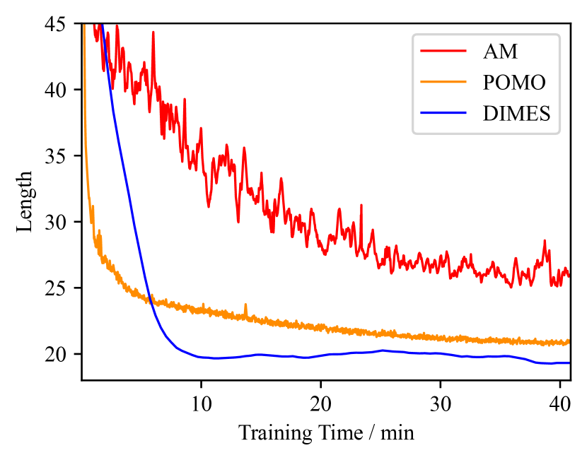
(a) Performance vs training time.

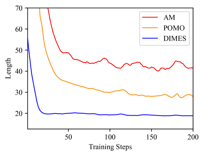
(b) Performance vs training steps.

Figure 1: Evaluation performance vs training cost.

F.3 Stability of Training

We compare the training settings of AM [42], POMO [45], and DIMES in Table 6. The training costs of AM and POMO are obtained from their papers A training step means a gradient descent step of the GNN. That is, for AM/POMO, a training step means a gradient descent step over a batch; for DIMES, a training step means a meta-gradient descent step.

The table shows that DIMES is much more sample-efficient than AM/POMO. Notably, DIMES achieves stable training using only 3 instances per meta-gradient descent step. Hence, its total training time is accordingly much shorter, even though its per-step time is longer. Moreover, the stability of training enables us to use a larger learning rate, which also accelerates training.

To further illustrate the fast stable training of DIMES, we compare the dynamics of training among AM, POMO, and DIMES in Figure 1. We closely follow the training settings of their papers, i.e., we train AM/POMO on TSP-100 and DIMES on TSP-500. For AM/POMO, we train their models on our hardware by re-running their public source code. The performance is evaluated using TSP-500 test instances. For DIMES, we use RL+S in evaluation.

From Figure 1(a), we can observe that DIMES stably converges to a better performance within fewer time, while the dynamics of training AM/POMO are slower and less stable. From Figure 1(b), we can observe that DIMES converges at much fewer training steps. The results again demonstrate that the training of DIMES is fast and stable.

References

- Ahn et al. [2020] Sungsoo Ahn, Younggyo Seo, and Jinwoo Shin. Learning what to defer for maximum independent sets. In International Conference on Machine Learning, pages 134–144. PMLR, 2020.
- Alkhouri et al. [2022] Ismail R Alkhouri, George K Atia, and Alvaro Velasquez. A differentiable approach to combinatorial optimization using dataless neural networks. arXiv preprint arXiv:2203.08209, 2022.
- Andrade et al. [2012] Diogo V Andrade, Mauricio GC Resende, and Renato F Werneck. Fast local search for the maximum independent set problem. Journal of Heuristics, 18(4):525–547, 2012.
- Applegate et al. [2006] David Applegate, Ribert Bixby, Vasek Chvatal, and William Cook. Concorde TSP solver. https://www.math.uwaterloo.ca/tsp/concorde/index.html, 2006.
- Arora [1996] Sanjeev Arora. Polynomial time approximation schemes for Euclidean TSP and other geometric problems. In Proceedings of 37th Conference on Foundations of Computer Science, pages 2–11. IEEE, 1996.
- Bellman [1962] Richard Bellman. Dynamic programming treatment of the travelling salesman problem. Journal of the ACM (JACM), 9(1):61–63, 1962.
- Bello et al. [2016] Irwan Bello, Hieu Pham, Quoc V Le, Mohammad Norouzi, and Samy Bengio. Neural combinatorial optimization with reinforcement learning. arXiv preprint arXiv:1611.09940, 2016.
- Böther et al. [2022] Maximilian Böther, Otto Kißig, Martin Taraz, Sarel Cohen, Karen Seidel, and Tobias Friedrich. What’s wrong with deep learning in tree search for combinatorial optimization. In International Conference on Learning Representations, 2022. URL https://openreview.net/forum?id=mk0HzdqY7i1.
- Bresson and Laurent [2018] Xavier Bresson and Thomas Laurent. An experimental study of neural networks for variable graphs. In ICLR 2018 Workshop, 2018.
- Chen and Tian [2019] Xinyun Chen and Yuandong Tian. Learning to perform local rewriting for combinatorial optimization. In Proceedings of the 33rd International Conference on Neural Information Processing Systems, pages 6281–6292, 2019.
- Croes [1958] Georges A Croes. A method for solving traveling-salesman problems. Operations research, 6(6):791–812, 1958.
- da Costa et al. [2020] Paulo R de O da Costa, Jason Rhuggenaath, Yingqian Zhang, and Alp Akcay. Learning 2-OPT heuristics for the traveling salesman problem via deep reinforcement learning. arXiv preprint arXiv:2004.01608, 2020.
- Deudon et al. [2018] Michel Deudon, Pierre Cournut, Alexandre Lacoste, Yossiri Adulyasak, and Louis-Martin Rousseau. Learning heuristics for the TSP by policy gradient. In International conference on the integration of constraint programming, artificial intelligence, and operations research, pages 170–181. Springer, 2018.
- Drori et al. [2020] Iddo Drori, Anant Kharkar, William R Sickinger, Brandon Kates, Qiang Ma, Suwen Ge, Eden Dolev, Brenda Dietrich, David P Williamson, and Madeleine Udell. Learning to solve combinatorial optimization problems on real-world graphs in linear time. In 2020 19th IEEE International Conference on Machine Learning and Applications (ICMLA), pages 19–24. IEEE, 2020.
- Elfwing et al. [2018] Stefan Elfwing, Eiji Uchibe, and Kenji Doya. Sigmoid-weighted linear units for neural network function approximation in reinforcement learning. Neural Networks, 107:3–11, 2018.
- Erdős et al. [1960] Paul Erdős, Alfréd Rényi, et al. On the evolution of random graphs. Publ. Math. Inst. Hung. Acad. Sci, 5(1):17–60, 1960.
- Fey and Lenssen [2019] Matthias Fey and Jan E. Lenssen. Fast graph representation learning with PyTorch Geometric. In ICLR Workshop on Representation Learning on Graphs and Manifolds, 2019.
- Finn et al. [2017] Chelsea Finn, Pieter Abbeel, and Sergey Levine. Model-agnostic meta-learning for fast adaptation of deep networks. In International Conference on Machine Learning, pages 1126–1135. PMLR, 2017.
- Fu et al. [2020] Zhang-Hua Fu, Kai-Bin Qiu, and Hongyuan Zha. Generalize a small pre-trained model to arbitrarily large TSP instances. arXiv preprint arXiv:2012.10658, 2020.
- Gonzalez [2007] Teofilo F Gonzalez. Handbook of approximation algorithms and metaheuristics. CRC Press, 2007.
- Gurobi Optimization [2018] LLC Gurobi Optimization. Gurobi optimizer reference manual, 2018.
- He et al. [2016] Kaiming He, Xiangyu Zhang, Shaoqing Ren, and Jian Sun. Deep residual learning for image recognition. In Proceedings of the IEEE conference on computer vision and pattern recognition, pages 770–778, 2016.
- Helsgaun [2017] K. Helsgaun. An extension of the Lin-Kernighan-Helsgaun TSP solver for constrained traveling salesman and vehicle routing problems. Technical report, Roskilde University, 2017.
- Helsgaun [2000] Keld Helsgaun. An effective implementation of the Lin–Kernighan traveling salesman heuristic. European journal of operational research, 126(1):106–130, 2000.
- Hoos and Stützle [2000] Holger H Hoos and Thomas Stützle. SATLIB: An online resource for research on SAT. Sat, 2000:283–292, 2000.
- Hottung and Tierney [2019] André Hottung and Kevin Tierney. Neural large neighborhood search for the capacitated vehicle routing problem. arXiv preprint arXiv:1911.09539, 2019.
- Hottung et al. [2020] André Hottung, Bhanu Bhandari, and Kevin Tierney. Learning a latent search space for routing problems using variational autoencoders. In International Conference on Learning Representations, 2020.
- Hottung et al. [2021] André Hottung, Yeong-Dae Kwon, and Kevin Tierney. Efficient active search for combinatorial optimization problems. arXiv preprint arXiv:2106.05126, 2021.
- Hudson et al. [2021] Benjamin Hudson, Qingbiao Li, Matthew Malencia, and Amanda Prorok. Graph neural network guided local search for the traveling salesperson problem. arXiv preprint arXiv:2110.05291, 2021.
- Ioffe and Szegedy [2015] Sergey Ioffe and Christian Szegedy. Batch normalization: Accelerating deep network training by reducing internal covariate shift. In International conference on machine learning, pages 448–456. PMLR, 2015.
- Joshi et al. [2019a] Chaitanya K Joshi, Thomas Laurent, and Xavier Bresson. An efficient graph convolutional network technique for the travelling salesman problem. arXiv preprint arXiv:1906.01227, 2019a.
- Joshi et al. [2019b] Chaitanya K Joshi, Thomas Laurent, and Xavier Bresson. On learning paradigms for the travelling salesman problem. arXiv preprint arXiv:1910.07210, 2019b.
- Joshi et al. [2020] Chaitanya K Joshi, Quentin Cappart, Louis-Martin Rousseau, Thomas Laurent, and Xavier Bresson. Learning tsp requires rethinking generalization. arXiv preprint arXiv:2006.07054, 2020.
- Karalias and Loukas [2020] Nikolaos Karalias and Andreas Loukas. Erdős goes neural: An unsupervised learning framework for combinatorial optimization on graphs. Advances in Neural Information Processing Systems, 33:6659–6672, 2020.
- Karp [1972] Richard M Karp. Reducibility among combinatorial problems. Complexity of Computer Computations, pages 85–103, 1972.
- Khalil et al. [2017] Elias Khalil, Hanjun Dai, Yuyu Zhang, Bistra Dilkina, and Le Song. Learning combinatorial optimization algorithms over graphs. Advances in Neural Information Processing Systems, 30:6348–6358, 2017.
- Kim et al. [2021] Minsu Kim, Jinkyoo Park, et al. Learning collaborative policies to solve NP-hard routing problems. Advances in Neural Information Processing Systems, 34, 2021.
- Kingma and Ba [2014] Diederik P Kingma and Jimmy Ba. Adam: A method for stochastic optimization. arXiv preprint arXiv:1412.6980, 2014.
- Kingma and Welling [2013] Diederik P Kingma and Max Welling. Auto-encoding variational Bayes. arXiv preprint arXiv:1312.6114, 2013.
- Kipf and Welling [2016] Thomas N Kipf and Max Welling. Semi-supervised classification with graph convolutional networks. arXiv preprint arXiv:1609.02907, 2016.
- Konda and Tsitsiklis [2000] Vijay R Konda and John N Tsitsiklis. Actor-critic algorithms. In Advances in neural information processing systems, pages 1008–1014, 2000.
- Kool et al. [2019a] Wouter Kool, Herke van Hoof, and Max Welling. Attention, learn to solve routing problems! In International Conference on Learning Representations, 2019a.
- Kool et al. [2019b] Wouter Kool, Herke van Hoof, and Max Welling. Buy 4 REINFORCE samples, get a baseline for free! In Deep Reinforcement Learning Meets Structured Prediction, ICLR 2019 Workshop, 2019b.
- Kool et al. [2021] Wouter Kool, Herke van Hoof, Joaquim Gromicho, and Max Welling. Deep policy dynamic programming for vehicle routing problems. arXiv preprint arXiv:2102.11756, 2021.
- Kwon et al. [2020] Yeong-Dae Kwon, Jinho Choo, Byoungjip Kim, Iljoo Yoon, Youngjune Gwon, and Seungjai Min. POMO: Policy optimization with multiple optima for reinforcement learning. arXiv preprint arXiv:2010.16011, 2020.
- Kwon et al. [2021] Yeong-Dae Kwon, Jinho Choo, Iljoo Yoon, Minah Park, Duwon Park, and Youngjune Gwon. Matrix encoding networks for neural combinatorial optimization. Advances in Neural Information Processing Systems, 34, 2021.
- LeCun et al. [2006] Yann LeCun, Sumit Chopra, Raia Hadsell, M Ranzato, and F Huang. A tutorial on energy-based learning. Predicting structured data, 1(0), 2006.
- Li et al. [2018] Zhuwen Li, Qifeng Chen, and Vladlen Koltun. Combinatorial optimization with graph convolutional networks and guided tree search. Advances in neural information processing systems, 31, 2018.
- Lin and Kernighan [1973] Shen Lin and Brian W Kernighan. An effective heuristic algorithm for the traveling-salesman problem. Operations research, 21(2):498–516, 1973.
- Loshchilov and Hutter [2019] Ilya Loshchilov and Frank Hutter. Decoupled weight decay regularization. In International Conference on Learning Representations, 2019.
- Lu et al. [2020] Hao Lu, Xingwen Zhang, and Shuang Yang. A learning-based iterative method for solving vehicle routing problems. In International Conference on Learning Representations, 2020.
- Ma et al. [2019] Qiang Ma, Suwen Ge, Danyang He, Darshan Thaker, and Iddo Drori. Combinatorial optimization by graph pointer networks and hierarchical reinforcement learning. arXiv preprint arXiv:1911.04936, 2019.
- Ma et al. [2021] Yining Ma, Jingwen Li, Zhiguang Cao, Wen Song, Le Zhang, Zhenghua Chen, and Jing Tang. Learning to iteratively solve routing problems with dual-aspect collaborative Transformer. Advances in Neural Information Processing Systems, 34, 2021.
- Moon and Moser [1965] John W Moon and Leo Moser. On cliques in graphs. Israel journal of Mathematics, 3(1):23–28, 1965.
- Nair and Hinton [2010] Vinod Nair and Geoffrey E Hinton. Rectified linear units improve restricted Boltzmann machines. In Icml, 2010.
- Nair et al. [2020] Vinod Nair, Sergey Bartunov, Felix Gimeno, Ingrid von Glehn, Pawel Lichocki, Ivan Lobov, Brendan O’Donoghue, Nicolas Sonnerat, Christian Tjandraatmadja, Pengming Wang, et al. Solving mixed integer programs using neural networks. arXiv preprint arXiv:2012.13349, 2020.
- Nazari et al. [2018] Mohammadreza Nazari, Afshin Oroojlooy, Lawrence V Snyder, and Martin Takáč. Reinforcement learning for solving the vehicle routing problem. arXiv preprint arXiv:1802.04240, 2018.
- Nichol et al. [2018] Alex Nichol, Joshua Achiam, and John Schulman. On first-order meta-learning algorithms. arXiv preprint arXiv:1803.02999, 2018.
- Ouyang et al. [2021] Wenbin Ouyang, Yisen Wang, Shaochen Han, Zhejian Jin, and Paul Weng. Improving generalization of deep reinforcement learning-based tsp solvers. arXiv preprint arXiv:2110.02843, 2021.
- Papadimitriou [1977] Christos H Papadimitriou. The Euclidean travelling salesman problem is NP-complete. Theoretical computer science, 4(3):237–244, 1977.
- Papadimitriou and Steiglitz [1998] Christos H Papadimitriou and Kenneth Steiglitz. Combinatorial optimization: algorithms and complexity. Courier Corporation, 1998.
- Paszke et al. [2019] Adam Paszke, Sam Gross, Francisco Massa, Adam Lerer, James Bradbury, Gregory Chanan, Trevor Killeen, Zeming Lin, Natalia Gimelshein, Luca Antiga, Alban Desmaison, Andreas Kopf, Edward Yang, Zachary DeVito, Martin Raison, Alykhan Tejani, Sasank Chilamkurthy, Benoit Steiner, Lu Fang, Junjie Bai, and Soumith Chintala. PyTorch: An imperative style, high-performance deep learning library. In H. Wallach, H. Larochelle, A. Beygelzimer, F. d'Alché-Buc, E. Fox, and R. Garnett, editors, Advances in Neural Information Processing Systems 32, pages 8024–8035. Curran Associates, Inc., 2019.
- Peng et al. [2019] Bo Peng, Jiahai Wang, and Zizhen Zhang. A deep reinforcement learning algorithm using dynamic attention model for vehicle routing problems. In International Symposium on Intelligence Computation and Applications, pages 636–650. Springer, 2019.
- Reeves [1997] Colin Reeves. Modern heuristics techniques for combinatorial problems. Nikkan Kogyo Shimbun, 1997.
- Shaw [1997] Paul Shaw. A new local search algorithm providing high quality solutions to vehicle routing problems. APES Group, Dept of Computer Science, University of Strathclyde, Glasgow, Scotland, UK, 46, 1997.
- Vaswani et al. [2017] Ashish Vaswani, Noam Shazeer, Niki Parmar, Jakob Uszkoreit, Llion Jones, Aidan N Gomez, Łukasz Kaiser, and Illia Polosukhin. Attention is all you need. In Advances in neural information processing systems, pages 5998–6008, 2017.
- Vesselinova et al. [2020] Natalia Vesselinova, Rebecca Steinert, Daniel F Perez-Ramirez, and Magnus Boman. Learning combinatorial optimization on graphs: A survey with applications to networking. IEEE Access, 8:120388–120416, 2020.
- Vinyals et al. [2015] Oriol Vinyals, Meire Fortunato, and Navdeep Jaitly. Pointer networks. Advances in Neural Information Processing Systems, 28:2692–2700, 2015.
- Wang et al. [2021a] Chenguang Wang, Yaodong Yang, Oliver Slumbers, Congying Han, Tiande Guo, Haifeng Zhang, and Jun Wang. A game-theoretic approach for improving generalization ability of TSP solvers. arXiv preprint arXiv:2110.15105, 2021a.
- Wang et al. [2021b] Runzhong Wang, Zhigang Hua, Gan Liu, Jiayi Zhang, Junchi Yan, Feng Qi, Shuang Yang, Jun Zhou, and Xiaokang Yang. A bi-level framework for learning to solve combinatorial optimization on graphs. arXiv preprint arXiv:2106.04927, 2021b.
- Williams [1992] Ronald J Williams. Simple statistical gradient-following algorithms for connectionist reinforcement learning. Machine learning, 8(3):229–256, 1992.
- Wu et al. [2021] Yaoxin Wu, Wen Song, Zhiguang Cao, Jie Zhang, and Andrew Lim. Learning improvement heuristics for solving routing problems.. IEEE Transactions on Neural Networks and Learning Systems, 2021.
- Xin et al. [2021a] Liang Xin, Wen Song, Zhiguang Cao, and Jie Zhang. Multi-decoder attention model with embedding glimpse for solving vehicle routing problems. In Proceedings of 35th AAAI Conference on Artificial Intelligence, 2021a.
- Xin et al. [2021b] Liang Xin, Wen Song, Zhiguang Cao, and Jie Zhang. NeuroLKH: Combining deep learning model with Lin–Kernighan–Helsgaun heuristic for solving the traveling salesman problem. Advances in Neural Information Processing Systems, 34, 2021b.
- Yolcu and Póczos [2019] Emre Yolcu and Barnabás Póczos. Learning local search heuristics for boolean satisfiability. In NeurIPS, pages 7990–8001, 2019.
- Zhang et al. [2020] Cong Zhang, Wen Song, Zhiguang Cao, Jie Zhang, Puay Siew Tan, and Chi Xu. Learning to dispatch for job shop scheduling via deep reinforcement learning. arXiv preprint arXiv:2010.12367, 2020.
- Zheng et al. [2020] Jiongzhi Zheng, Kun He, Jianrong Zhou, Yan Jin, and Chu-Min Li. Combining reinforcement learning with Lin–Kernighan–Helsgaun algorithm for the traveling salesman problem. arXiv preprint arXiv:2012.04461, 2020.