The UV Excesses of Supernovae and the Implications for Studying Supernovae and Other Optical Transients

Tao Wang (王涛) Guangxi Key Laboratory for Relativistic Astrophysics, School of Physical Science and Technology, Guangxi University, Nanning 530004, China Shan-Qin Wang (王善钦) Guangxi Key Laboratory for Relativistic Astrophysics, School of Physical Science and Technology, Guangxi University, Nanning 530004, China Wen-Pei Gan (甘文沛) Guangxi Key Laboratory for Relativistic Astrophysics, School of Physical Science and Technology, Guangxi University, Nanning 530004, China Nanjing Institute of Astronomical Optics & Technology, Nanjing 210042, China

Abstract

Supernovae (SNe), kilonovae (KNe), tidal disruption events (TDEs), optical afterglows of gamma ray bursts (GRBs), and many other optical transients are important phenomena in time-domain astronomy. Fitting the multi-band light curves (LCs) or the synthesized (pseudo-)bolometric LCs can be used to constrain the physical properties of optical transients. The (UV absorbed) blackbody module is one of the most important modules used to fit the multi-band LCs of optical transients having (UV absorbed) blackbody spectral energy distributions (SEDs). We find, however, that the SEDs of some SNe show UV excesses, which cannot be fitted by the model including a (UV absorbed) blackbody module. We construct the bolometric LCs and employ the (cooling plus) ⁵⁶Ni model to fit the constructed bolometric LCs, obtaining decent fits. Our results demonstrate that the optical transients showing UV excesses cannot be fitted by the multi-band models that include (UV-absorbed) blackbody module, but can be well modeled by constructing and fitting their bolometric LCs.

general – supernovae: individual (SN 2010jr, SN 2012au, SN 2013ak, SN 2013df, SN 2014ad)

1 Introduction

In the past two decades, the wide-field optical survey telescopes discovered supernovae (SNe), kilonovae (KNe), tidal disruption events (TDEs), optical afterglows of Gamma-ray bursts (GRBs), and other optical transients. To constrain the physical properties of the optical transients, the method of fitting the multi-band light curves (LCs) is widely adopted to model the photometry of superluminous SNe (Nicholl et al., 2017b; Moriya et al., 2018), stripped-envelope SNe (Zheng et al., 2022), TDEs (Mockler et al., 2019), KNe (Villar et al., 2017), and (super)luminous rapidly evolving optical transients or SNe (Wang et al., 2019; Wang & Gan, 2022).

The (UV absorbed) blackbody module (e.g., Chomiuk et al. 2011; Nicholl et al. 2017a, b; Prajs et al. 2017) is one of the most important modules used to fit the multi-band LCs of optical transients, since the spectral energy distributions (SEDs) of the optical transients listed above (except for the optical afterglows of GRBs) can be approximately described by the (UV absorbed) blackbody function.

In this paper, we demonstrate that the SEDs of five SNe (SN 2010jr, SN 2012au, SN 2013ak, SN 2013df, and SN 2014ad) show UV excesses which cannot be described by UV absorbed blackbody or standard blackbody function. The UV-optical LCs cannot be fitted by the multi-band model, while the optical photometry can be well fitted by the same model.

To better constrain the physical properties, we construct and model the bolometric LCs of the five SNe, getting good fits. In Section 2, we demonstrate that the UV-optical SEDs of the five SNe show UV excesses by fitting the SEDs and multi-band LCs. In Section 3, we construct and model the bolometric LCs of the five SNe. We discuss our results and draw some conclusions in Section 4. Throughout the paper, we assume $\Omega_{m}=0.315$ , $\Omega_{\Lambda}=0.685$ , and H ${}_{0}=67.3$ km s^-1 Mpc^-1 (Planck Collaboration, 2014). The values of the Milky Way reddening ( $E_{\mathrm{B-V}}$ ) of all events are from Schlafly & Finkbeiner (2011).

2 The SED and LC Fits

The photometric data and the detailed information (e.g., the positions, SN types, the values of their redshifts, and so on) of the five SNe, SN 2010jr, SN 2012au, SN 2013ak, SN 2013df, and SN 2014ad, are from Brown et al. (2014), Milisavljevic et al. (2013), Brown et al. (2014), Morales-Garoffolo et al. (2014); Brown et al. (2014), and Sahu et al. (2018) via the collection of Open Supernova Catalog (Guillochon et al., 2017), respectively.

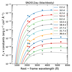
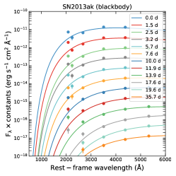
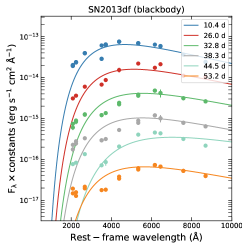
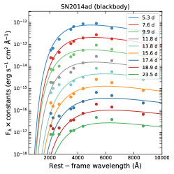
First, we use the standard blackbody function ( $F_{\nu}=(2\pi h\nu^{3}/c^{2})(e^{{h\nu}/{k_{b}T_{\rm ph}}}-1)^{-1}\frac{R_{\rm ph}^{2}}{D^{2}_{\rm L}}$ , $T_{\rm ph}$ is the temperature of the SN photosphere, $R_{\rm ph}$ is the radius of the SN photosphere, $D_{\rm L}$ is the luminosity distance of the SN) to fit their UV-optical SEDs at all epochs, see Figure 1. ¹¹1The linear interpolation is performed in some epochs to obtain the SEDs at the same epochs. We don’t include some optical photometric data of SN 2013df at 150-250 d, since they cannot be used to construct SEDs.

We find that the SEDs at all epochs (for SN 2012au, SN 2013ak, and SN 2013df) or the late epochs (for SN 2010jr and SN 2014ad) of the SNe show UV excesses relative to the standard blackbody model. The UV excesses of the SEDs indicate that the UV-optical photometry cannot be fitted by the multi-band model that includes the standard or UV absorbed blackbody assumption.

To support the statements above, we adopt the ⁵⁶Ni or the cooling plus ⁵⁶Ni model to fit the LCs of the three single-peaked SNe (SN 2012au, SN 2013ak, and SN 2014ad) and the two double-peaked SNe (SN 2010jr and SN 2013df), respectively. ²²2Since they are stripped-envelope SNe (IIb, Ib and Ic) with normal peak luminosities, the energy from the recombination of the ionized hydrogen or the magnetar spinning-down can be neglected. The details of the ⁵⁶Ni model can be found in the references of Wang & Gan (2022), while the details of the cooling model can be found in Piro et al. (2021).

The values of the optical opacity of the ejecta $\kappa$ and the $\gamma$ -ray opacity $\kappa_{\gamma}$ are set to be 0.07 cm²g^-1 and 0.027 cm²g^-1, respectively. The free parameters of the ⁵⁶Ni model adopted here are the ejecta mass M_ej, the ejecta velocity $v_{\rm ph}$ , ³³3The photospheric velocity of SN 2012au, SN 2013ak, and SN 2013df determined by the spectral lines are set to be the upper limits of their $v_{\rm ph}$ , see Table LABEL:Tab. the ⁵⁶Ni mass M_Ni, the temperature floor of the photosphere T_f, the explosion time relative to the first data t_shift. ⁴⁴4The date of the first photometric data of every SN is set to be the day 0. The additional parameters required by the cooling plus ⁵⁶Ni model are the extended material mass M_e, the extended material radius R_e, the energy imparted by the shock passing through the extended material E_e.

The Markov Chain Monte Carlo (MCMC) using the emcee Python package (Foreman-Mackey et al., 2013) is adopted to get the best-fitting parameters. We employ 20 walkers, each walker runs 30,000 steps. The uncertainties are 1 $\sigma$ confidence, corresponding to the 16th and 84th percentiles of the posterior samples.

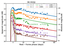
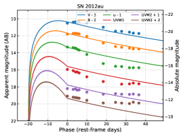
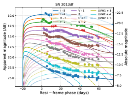
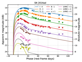
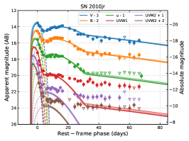
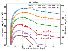
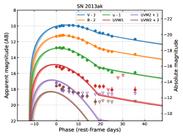
The multi-band LC fits of the five SNe are shown in Figure 2, and the corresponding optimal parameters are shown in Table LABEL:Tab. We find that the LCs of SN 2010jr and SN 2012au at all bands cannot be fitted, the LCs of SN 2013df at optical bands and $U/u$ cannot be fitted, the optical LCs of SN 2013ak and SN 2014ad can be fitted while their UV LCs show UV excesses in $UVW1$ and $UVW2$ or $UVW1$ , $UVM2$ , and $UVW2$ bands at some epochs.

Alternatively, we use the same models to fit the optical and $U/u$ LCs of the five SNe, see Figure 3 (the $UVW1$ -, $UVM2$ -, and $UVW2$ -band photometry are also plotted, but not fitted) and Table LABEL:Tab for the fits and the best-fit parameters, respectively. We find that the optical and $U/u$ LCs of SN 2010jr, SN 2012au, and SN 2013df can be well fitted, while the $UVW1$ -, $UVM2$ -, and $UVW2$ -bands show apparent UV excesses at most epochs. Compared to the fits for the data sets in all bands, the fits for SN 2013ak and SN 2014ad do not change significantly, because the weight of the data in $UVW1$ -, $UVM2$ -, and $UVW2$ -bands is significantly lower than that of the optical and $U/u$ bands.

The fits for two different data sets (all bands versus optical and $U/u$ bands) also indicate that the SEDs of the all five SNe show UV excesses, and that the LCs cannot be fitted by the multi-band models (since the $UVW1$ -, $UVM2$ -, and $UVW2$ -band data cannot be fitted).

3 Constructing and Fitting the bolometric LCs

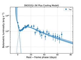
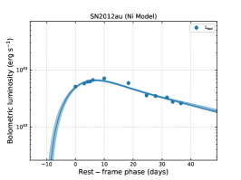
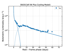
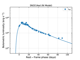
To constrain the physical properties of the SNe, we must synthesize and fit the bolometric LCs. To avoid missing the UV and IR flux, we first divide the area under a theoretical SED into three classes: (1) The part between 0 to the $\lambda_{\rm UVW2}$ is assumed to be a triangle; (2) the part between the $\lambda_{\rm UVW2}$ to $\lambda_{\rm u}$ are assumed to be several trapezoids; (3) the part of a SED longer than $\lambda_{\rm u}$ is described by the blackbody fit ( $f_{\nu,\lambda>\lambda_{\rm u}}=(2\pi h\nu^{3}/c^{2})(e^{{h\nu}/{k_{b}T_{\rm ph}}}-1)^{-1}\frac{R_{\rm ph}^{2}}{D^{2}_{\rm L}}$ ). We integrate the three parts of the SEDs and get the flux at all epochs, i.e., $f=\int_{0}^{\infty}f_{\nu}d{\nu}=\int_{0}^{\lambda_{\rm UVW2}}f_{\nu}d\nu+\int_{\lambda_{\rm UVW2}}^{\lambda_{\rm u}}f_{\nu}d\nu+\int_{\lambda_{\rm u}}^{\infty}f_{\nu}d\nu$ . The bolometric luminosities can be calculated by $L_{\rm bol}=4{\pi}D^{2}_{\rm L}f$ . ⁵⁵5The SEDs of SN 2014ad after day 23 do not have $u$ , $UVW1$ , $UVM2$ , and $UVW2$ photometry. We roughly assume that the ratio of the luminosity of the part between 0 to $\lambda_{\rm u}$ to bolometric luminosity is constant ( $\sim$ 6% which is the mean value derived from the integration for the early-epoch SEDs). The synthesized bolometric LCs of the five SNe are shown in Figure 4.

The parameters of ⁵⁶Ni model used to fit the bolometric LCs of SN 2012au, SN 2013ak, and SN 2014ad and the cooling plus ⁵⁶Ni model used to fit the bolometric LCs of SN 2010jr and SN 2013df are listed in Table LABEL:Tab. The bolometric LC fits and the best-fit parameters are shown in Figure 4 and Table LABEL:Tab, respectively. We find that the bolometric LCs can be well fitted by the models and the values of $\chi^{2}/$ dof (dof=degree of freedom) are significantly smaller than the multi-band LC fits (see the last column of Table LABEL:Tab). This indicates that the method of synthesizing and fitting the bolometric LCs is the best one for the SNe showing UV excesses.

It should be noted that, however, the synthesized bolometric LC of SN 2014ad around the peak show undulation feature (see Figure 4). This is due to the undulation of the photometric data in $UVW1$ , $UVM2$ , and $UVW2$ bands (see Figures 2 and 3). The undulation results in a large $\chi^{2}/$ dof. Nevertheless, the value of $\chi^{2}/$ dof of the fit of the bolometric LC is significantly smaller than that of the fit of the multi-band LCs.

4 Discussion and Conclusions

In this paper, we demonstrate that the SEDs of five SNe show UV excesses by fitting their SEDs and the multi-band LCs. We suggest that the five SNe and other optical transients having UV excesses cannot be fitted by the multi-band models including a UV-absorbed or standard blackbody module.

To constrain the physical properties of the SNe showing UV excesses, we construct and fit their bolometric LCs, getting decent fits. Moreover, the bolometric LC fits are significantly better than the multi-band fits. Our results indicate that the most reasonable scheme of deriving the physical properties of the optical transients having UV excesses might be constructing and fitting the bolometric LCs, because the multi-band LCs cannot be fitted.

It is important to emphasize that the multi-band models including a (UV-absorbed) blackbody module are still the best ones to fit the optical transients which show UV absorption or have very few or no UV data. In fact, the reliable bolometric LCs are difficult to be constructed for the optical transients with sparse or no UV data.

Currently, only a small fraction of SNe, TDEs, and other optical transients have been observed in UV bands shorter than 3000 Å. In the future, the Large Synoptic Survey Telescope (LSST) and other large survey telescope would obtain the far UV photometry of numerous optical transients at high redshifts (e.g., $z\gtrsim 1$ ) using the optical filters, since the flux in some UV bands would be redshifted and become optical flux observed. Therefore, we can expect that the large optical survey telescopes would discover a great number of optical transients showing UV excesses, which cannot be fitted by the multi-band models that include (UV-absorbed) blackbody module, but can be well modeled by constructing and fitting their bolometric LCs.

This work is supported by National Natural Science Foundation of China (grant 11963001).

References

Brown et al. (2014) Brown, P. J., Breeveld, A. A., Holland, S., Kuin, P., & Pritchard, T. 2014, Ap&SS, 354, 89
Carrasco et al. (2013) Carrasco, F., Hamuy, M., Antezana, R., et al. 2013, Central Bureau Electronic Telegrams, 3437, 1
Chomiuk et al. (2011) Chomiuk, L., Chornock, R., Soderberg, A., et al. 2011, ApJ, 743, 114
Foreman-Mackey et al. (2013) Foreman-Mackey, D., Hogg, D. W., Lang, D., & Goodman, J. 2013, PASP, 125, 306
Guillochon et al. (2017) Guillochon, J., Parrent, J., Kelley, L. Z., & Margutti, R. 2017, ApJ, 835, 64
Milisavljevic et al. (2013) Milisavljevic, D., Soderberg, A. M., Margutti, R., et al. 2013, ApJ, 770, L38
Mockler et al. (2019) Mockler, B., Guillochon, J., & Ramirez-Ruiz, E. 2019, ApJ, 872, 151
Morales-Garoffolo et al. (2014) Morales-Garoffolo, A., Elias-Rosa, N., Benetti, S., et al. 2014, MNRAS, 445, 1647
Moriya et al. (2018) Moriya, T. J., Nicholl, M., & Guillochon, J. 2018, ApJ, 867, 113
Nicholl et al. (2017a) Nicholl, M., Berger, E., Margutti, R., et al. 2017a, ApJ, 835, L8
Nicholl et al. (2017b) Nicholl, M., Guillochon, J., & Berger, E. 2017b, ApJ, 850, 55
Pandey et al. (2021) Pandey, S. B., Kumar, A., Kumar, B., et al. 2021, MNRAS, 507, 1229
Piro et al. (2021) Piro, A. L., Haynie, A., & Yao, Y. 2021, ApJ, 909, 209
Planck Collaboration (2014) Planck Collaboration, Ade, P. A. R., Aghanim, N., Armitage-Caplan, C., et al. 2014, A&A, 571, A16
Prajs et al. (2017) Prajs, S., Sullivan, M., Smith, M., et al. 2017, MNRAS, 464, 3568
Sahu et al. (2018) Sahu, D. K., Anupama, G. C., Chakradhari, N. K., et al. 2018, MNRAS, 475, 2591
Schlafly & Finkbeiner (2011) Schlafly, E. F., & Finkbeiner, D. P. 2011, ApJ, 737, 103
Villar et al. (2017) Villar, V. A., Guillochon, J., Berger, E., et al. 2017, ApJ, 851, L21
Wang & Gan (2022) Wang, S.-Q., & Gan, W.-P. 2022, ApJ, 928, 114
Wang et al. (2019) Wang, S.-Q., Gan, W.-P., Li, L., et al. 2019, arXiv:1904.09604
Zheng et al. (2022) Zheng, W., Stahl, B. E., de Jaeger, T., et al. 2022, MNRAS, 512, 3195

Table 1: The best fitting parameters of the multi-band and bolometric LC models.

Name	M_e	R_e	lgE_e,50	M_ej	$v_{\rm ph}$	M_Ni	T_f	t_shift	$\chi^{2}/$ dof
unit	(M_⊙)	(R_⊙)	( $10^{50}\rm erg$ )	(M_⊙)	( $10^{9}\rm cm\ s^{-1}$ )	(M_⊙)	(K)	(day)
Prior	[0.01,20]	[10,3000]	[-3,3]	[0.1,50]	[0.1,A^a]	[0.001,2]	[1000,10000]	[-20,0]
parameters of multi-band LC fits
SN 2010jr	0.04 ${}^{+0.00}_{-0.00}$	121.49 ${}^{+45.63}_{-35.60}$	-0.67 ${}^{+0.12}_{-0.11}$	1.58 ${}^{+0.06}_{-0.06}$	0.91 ${}^{+0.03}_{-0.03}$	0.05 ${}^{+0.00}_{-0.00}$	6406.92 ${}^{+44.73}_{-43.18}$	-4.87 ${}^{+0.39}_{-0.37}$	3.99
SN 2012au	-	-	-	1.84 ${}^{+0.04}_{-0.04}$	1.25 ${}^{+0.00}_{-0.01}$	0.27 ${}^{+0.00}_{-0.00}$	6524.76 ${}^{+12.97}_{-13.28}$	-19.89 ${}^{+0.10}_{-0.05}$	60.52
SN 2013ak	-	-	-	3.38 ${}^{+0.11}_{-0.11}$	1.33 ${}^{+0.04}_{-0.04}$	0.27 ${}^{+0.00}_{-0.00}$	4168.13 ${}^{+45.77}_{-42.59}$	-12.39 ${}^{+0.49}_{-0.49}$	10.46
SN 2013df	1.97 ${}^{+0.01}_{-0.01}$	439.65 ${}^{+4.06}_{-4.16}$	0.01 ${}^{+0.01}_{-0.01}$	0.33 ${}^{+0.04}_{-0.03}$	0.01 ${}^{+0.00}_{-0.00}$	0.01 ${}^{+0.00}_{-0.00}$	5491.97 ${}^{+3050.79}_{-3044.92}$	-19.93 ${}^{+0.10}_{-0.05}$	67.68
SN 2014ad	-	-	-	3.05 ${}^{+0.01}_{-0.01}$	1.23 ${}^{+0.00}_{-0.00}$	0.20 ${}^{+0.00}_{-0.00}$	4498.80 ${}^{+2.71}_{-2.69}$	-9.77 ${}^{+0.04}_{-0.04}$	650.11
parameters of multi-band LC fits (excluding $UVW1$ , $UVM2$ , and $UVW2$ bands
SN 2010jr	0.05 ${}^{+0.01}_{-0.00}$	63.41 ${}^{+22.95}_{-17.90}$	-0.39 ${}^{+0.13}_{-0.10}$	5.24 ${}^{+0.43}_{-0.40}$	1.13 ${}^{+0.07}_{-0.07}$	0.12 ${}^{+0.01}_{-0.01}$	3738.79 ${}^{+71.25}_{-67.01}$	-4.33 ${}^{+0.43}_{-0.46}$	42.92
SN 2012au	-	-	-	3.72 ${}^{+0.13}_{-0.13}$	1.24 ${}^{+0.01}_{-0.02}$	0.35 ${}^{+0.01}_{-0.01}$	4341.63 ${}^{+29.95}_{-29.60}$	-18.04 ${}^{+0.49}_{-0.53}$	460.30
SN 2013ak	-	-	-	3.01 ${}^{+0.16}_{-0.16}$	1.65 ${}^{+0.07}_{-0.07}$	0.31 ${}^{+0.01}_{-0.01}$	4165.86 ${}^{+47.82}_{-49.10}$	-11.92 ${}^{+0.51}_{-0.57}$	12.68
SN 2013df	0.05 ${}^{+0.00}_{-0.00}$	167.26 ${}^{+18.84}_{-16.58}$	-0.41 ${}^{+0.04}_{-0.04}$	1.95 ${}^{+0.02}_{-0.02}$	0.84 ${}^{+0.01}_{-0.01}$	0.11 ${}^{+0.00}_{-0.00}$	4150.27 ${}^{+7.02}_{-6.80}$	-1.97 ${}^{+0.08}_{-0.08}$	204.13
SN 2014ad	-	-	-	2.50 ${}^{+0.01}_{-0.01}$	1.15 ${}^{+0.00}_{-0.00}$	0.22 ${}^{+0.00}_{-0.00}$	4510.48 ${}^{+2.88}_{-2.92}$	-11.88 ${}^{+0.05}_{-0.04}$	650.29
parameters of bolometric LC fits
SN 2010jr	0.01 ${}^{+0.01}_{-0.00}$	478.05 ${}^{+593.66}_{-339.60}$	-2.08 ${}^{+0.82}_{-0.54}$	3.71 ${}^{+1.06}_{-1.23}$	1.67 ${}^{+0.24}_{-0.41}$	0.09 ${}^{+0.00}_{-0.01}$	-	-2.78 ${}^{+2.14}_{-0.87}$	1.18
SN 2012au	-	-	-	2.70 ${}^{+0.42}_{-0.53}$	1.12 ${}^{+0.10}_{-0.18}$	0.31 ${}^{+0.01}_{-0.01}$	-	-10.08 ${}^{+0.78}_{-0.88}$	1.72
SN 2013ak	-	-	-	4.20 ${}^{+1.00}_{-1.05}$	1.62 ${}^{+0.17}_{-0.30}$	0.32 ${}^{+0.02}_{-0.02}$	-	-10.52 ${}^{+1.04}_{-1.22}$	0.53
SN 2013df	0.03 ${}^{+0.01}_{-0.00}$	279.51 ${}^{+116.25}_{-91.36}$	-1.38 ${}^{+0.26}_{-0.23}$	1.26 ${}^{+0.04}_{-0.04}$	0.71 ${}^{+0.02}_{-0.02}$	0.09 ${}^{+0.00}_{-0.00}$	-	-0.03 ${}^{+0.02}_{-0.05}$	20.74
SN 2014ad	-	-	-	1.66 ${}^{+0.05}_{-0.05}$	0.91 ${}^{+0.02}_{-0.02}$	0.18 ${}^{+0.00}_{-0.00}$	-	-7.97 ${}^{+0.07}_{-0.07}$	174.86

^a Note. For SN 2010jr and SN 2014ad, A $=5$ ; for SN 2012au, A $=1.25$ (Pandey et al., 2021); for SN 2013ak A $=1.85$ (Carrasco et al., 2013); for SN 2013df, A $=0.9$ (Morales-Garoffolo et al., 2014).

Refer to caption — Figure 1: The best fits of the SEDs of the SNe at different epochs.