Leveraging progressive model and overfitting for efficient learned image compression

Abstract

Deep learning is overwhelmingly dominant in the field of computer vision and image/video processing for the last decade. However, for image and video compression, it lags behind the traditional techniques based on discrete cosine transform (DCT) and linear filters. Built on top of an auto-encoder architecture, learned image compression (LIC) systems have drawn enormous attention in recent years. Nevertheless, the proposed LIC systems are still inferior to the state-of-the-art traditional techniques, for example, the Versatile Video Coding (VVC/H.266) standard, due to either their compression performance or decoding complexity. Although claimed to outperform the VVC/H.266 on a limited bit rate range, some proposed LIC systems take over 40 seconds to decode a 2K image on a GPU system. In this paper, we introduce a powerful and flexible LIC framework with multi-scale progressive (MSP) probability model and latent representation overfitting (LOF) technique. With different predefined profiles, the proposed framework can achieve various balance points between compression efficiency and computational complexity. Experiments show that the proposed framework achieves 2.5%, 1.0%, and 1.3% Bjontegaard delta bit rate (BD-rate) reduction over the VVC/H.266 standard on three benchmark datasets on a wide bit rate range. More importantly, the decoding complexity is reduced from $O(n)$ to $O(1)$ compared to many other LIC systems, resulting in over 20 times speedup when decoding 2K images.

I Introduction

Although deep learning-based technology has achieved tremendous success in most computer vision and image/video processing tasks, it has not been able to demonstrate superior performance over traditional technologies for image and video compression, in particular, for practical usage. Traditional image compression techniques, such as JPEG/JPEG 2000 [1], High Efficiency Video Coding (HEVC) (all-intra mode) [2], and Versatile Video Coding (VVC/H.266) (all-intra mode) [3], apply carefully designed processing steps such as data transformation, quantization, entropy coding to compress the image data while maintaining certain quality for human perception [4, 5, 6]. End-to-end learned image compression (LIC) systems are based on deep learning technology and data-driven paradigm [7, 8, 9, 10, 11, 12, 13, 14, 15, 4, 16, 17]. These systems normally adopt the variational auto-encoder architecture, as shown in Figure 1, comprising encoder, decoder and probability model implemented by deep convolutional neural networks (CNN) [7, 18, 8, 9, 10, 11, 12, 13, 14]. LIC systems are trained on datasets with a large number of natural images by optimizing a rate-distortion (RD) loss function.

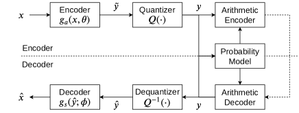
Figure 1: LIC architecture.

Compared with the state-of-the-art traditional image compression technologies, for example, VVC/H.266, most LIC systems do not provide better compression performance despite a much higher encoding and decoding complexity [19, 4, 14]. Recently, some proposed LIC systems have improved the compression performance to be on par with or slightly better than the VVC/H.266 [20, 21, 9, 22, 23, 24] on a limited bit rate range. However, the decoding procedures of these systems are very inefficient which prevents them from being used in practice.

In this paper, we propose a flexible and novel LIC framework that achieves various balance points between compression efficiency and computational complexity. A system based on the proposed frame outperforms the VVC/H.266 on three benchmarking datasets over a wide bit rate range. Compared to most other LIC systems, the proposed system not only improves the compression performance but also reduces the decoding complexity from $O(n)$ to $O(1)$ in a parallel computing environment. Our contributions are summarized as follows:

• We propose the multi-scale progressive (MSP) probability model for lossy image compression that efficiently exploits both spatial and channel correlation of the latent representation and significantly reduces decoding complexity.

• We present a greedy search method in applying the latent representation overfitting (LOF) technique and show that LOF can considerably improve the performance of LIC systems and mitigate the domain-shift problem.

II LIC system and related works

In [7], the authors formulated the LIC codec, named as transform coding model, from the generative Bayesian model. Figure 1 shows the architecture of a typical LIC codec. Input data $x$ is transformed by an analysis function $g_{a}\left(x;\theta\right)$ to generate a latent representation $\tilde{y}$ in continuous domain. Next, $\tilde{y}$ is quantized to latent representation $y$ in discrete domain. Then, the arithmetic encoder encodes $y$ into a bitstream using the estimated distribution provided by the probability model. The encoder operation can be represented by the function

$$y=Q\left(g_{a}\left(x;\theta\right)\right).$$ (1)

At the decoder side, an arithmetic decoder reconstructs $y$ from the bitstream with the help of the same probability model that is used at the encoder side. Next, $y$ is dequantized and a synthesis function $g_{s}\left(y;\phi\right)$ is used to generate $\hat{x}$ as the reconstructed input data. $g_{a}(\cdot;\theta)$ and $g_{s}\left(\cdot;\phi\right)$ are implemented using deep neural networks with parameters $\theta$ and $\phi$, respectively. The codec is trained by optimizing the RD loss function defined by

$$L =R\left(y\right)+\lambda\cdot D\left(x,\hat{x}\right)$$ (2)

$$=\mathbb{E}_{x\sim p(x)}\left[-\log p\left(y\right)\right]+\lambda\cdot\mathbb{E}_{x\sim p(x)}\left[d\left(x,\hat{x}\right)\right]$$ (3)

In Eq. 2, $R(y)$ is the rate loss measuring the expected number of bits to encode $y$, $D\left(x,\hat{x}\right)$ is the expected reconstruction loss measuring the quality of the reconstructed image, and $\lambda$ is the Lagrange multiplier that adjusts the weighting of the two loss terms to achieve difference compression rate. In Eq. 3, $p\left(y\right)$, also known as prior distribution, is the probability distribution of latent representation $y$, $d\left(x,\hat{x}\right)$ is the distance function measuring the quality of the reconstructed data $\hat{x}$, where MSE or MS-SSIM is normally used as the reconstruction loss [4, 25]. The RD loss function is a weighted sum of the expected bitstream length and the reconstructed loss.

The rate loss $R\left(y\right)$ is calculated by the expected length of the bitstream to encode latent representation $y$ when input data $x$ is compressed. Let $q\left(y\right)$ be the true distribution of $y$. Although $y$ is deterministic over random variable $x$ according to Eq. 1, $q\left(y\right)$ is still unknown since the true distribution of $x$ is unknown. To tackle this problem, an LIC codec uses a variational distribution $p\left(y\right)$, either a parametric model from a known distribution family [18, 26, 8, 20, 9, 22, 11, 27] or a non-parametric model [7], to replace $q\left(y\right)$ in calculating the rate loss. The rate loss is then calculated as the cross-entropy between $q\left(y\right)$ and $p\left(y\right)$, such as

$$R\left(y\right) =H\left(q\left(y\right),p\left(y\right)\right)$$ (4)

$$=\mathbb{E}_{y\sim q\left(y\right)}\left[-\log p\left(y\right)\right]$$ (5)

$$=H\left(q\left(y\right)\right)+D_{KL}\left(q\left(y\right)\parallel p\left(y\right)\right).$$ (6)

In [7], the authors model the prior distribution $p\left(y\right)$ as fully factorized where the distribution of each element is modeled non-parametrically using piece-wise linear functions. This simple model does not capture spatial dependencies in the latent representation. In [18], the authors introduced the scale hyperprior model, where the elements in the latent representation are modeled as independent zero-mean Gaussian distributions and the variance of each element is derived from side information $z$. $z$ is modeled using a different distribution model and transferred separately. The loss function becomes

$$L=R\left(y\right)+R\left(z\right)+\lambda D\left(x,\hat{x}\right).$$ (7)

In [11], the authors improved the scale hyperprior model from two aspects. First, both the mean and the variance of the Gaussian model are derived from the side information $z$, named as mean-scale hyperprior model. Second, a context model is introduced to further exploit the spatial dependencies of the elements. The context model uses the elements that have already been decoded to improve the model accuracy of the current element. A similar technique was used in image generative models such as PixelCNN [28, 29, 30]. Many recent LIC systems are based on the hyperprior architecture and the context model. The authors in [8] use mixture of Gaussian distributions instead of the Gaussian distribution in the mean-scale hyperprior model. In [20], the authors further apply mixture of Gaussian-Lapalacian-Logistic (GLL) distribution to model the latent representation. In [26], the authors enhance the context model by exploiting the channel dependencies. The parameters of the distribution function of the elements in $y$ are derived from the channels that have already been decoded. A 3D masked CNN is used to improve computational throughput. In [9], the authors divide the channels into two groups, where the first group is decoded in the same way as the normal context model and the second group is decoded using the first group as its context. With this architecture, the pixels in the second group are able to use the long-range correlation in $y$ since the first group is fully decoded. In [17], the authors proposed a method that partitions the elements in the latent representation into two groups along the spatial dimension in a checkerboard pattern. The elements in the first group are used as the context for the elements in the second group.

The context model, inspired by PixelCNN, exploits the spatial and channel correlation further. Although the encoding can be performed in a batch mode, the main issue of the PixelCNN-based context model is that the decoding has to be performed in sequential order, i.e., pixel by pixel, or even element by element if the channel dependency is exploited. According to the evaluation reported in [19], in an environment with GPUs, the average decoding time of Cheng2020 model [8] is 5.9 seconds per image with a resolution of $512\times 768$ and 45.9 seconds per image with an average resolution of $1913\times 1361$. To achieve better compression performance, recent LIC systems are even multiple times slower than the Cheng2020 system [20, 9, 22]. Furthermore, to avoid excessive computational complexity, the context model is implemented with a small neural network with a limited receptive field, which greatly degrades the system performance. The hyperprior architecture also tries to capture the spatial correlation in the latent representation. However. this architecture significantly increases the system complexity, for example, a 4-layer context model network and a 5-layer hyperpior decoder network are used in [8].

In this paper, we propose a LIC framework using a novel probability model which significantly improves the compression performance and decoding efficiency. Table I summarizes previously proposed LIC systems and the proposed system in this paper. In the table, full channel dependency mode means that each channel is dependent on all previous channels. Group dependency mode means that the channels are divided into groups and the channel dependency modes are different in each group or between groups. The decoding complexity measures the complexity of decoding operation in a parallel computing environment. $n$ is the number of pixels in the latent representation, $c$ is the number of channels. $O\left(1\right)$ means all pixels can be processed in parallel in a constant number of steps.

TABLE I: Comparison of the proposed method to prior works, in terms of characteristics and complexity of the probability model.

method	Hyperpior architecture	Distribution model	Context Model	Channel Dependency	Decoding complexity
Balle2017 [7]	No	non-parametric	No	None	$O\left(1\right)$
Balle2018 [18]	Yes	$\mathcal{N}\left(0,\sigma^{2}\right)$	No	None	$O\left(1\right)$
Minnen2018 [11]	Yes	$\mathcal{N}\left(\mu,\sigma^{2}\right)$	PixelCNN	None	$O\left(n\right)$
Chen2019 [26]	Yes	$\mathcal{N}\left(\mu,\sigma^{2}\right)$	PixelCNN	Full	$O\left(cn\right)$
Cheng2020 [8]	Yes	Gaussian mixture	PixelCNN	None	$O\left(n\right)$
He2021 [17]	Yes	Gaussian mixture	Checkerboard	None	$O\left(1\right)$
Fu2021 [20]	Yes	GLL mixture	PixelCNN	None	$O\left(n\right)$
Ma2021 [22]	Yes	$\mathcal{N}\left(\mu,\sigma^{2}\right)$	PixelCNN	Group	$O\left(kn\right)$†
Guo2021 [9]	Yes	Gaussian mixture	PixelCNN	Full	$O\left(cn\right)$
Proposed	No	$\mathcal{N}\left(\mu,\sigma^{2}\right)$	MSP	Group	$O\left(1\right)$ ‡

†: $k=c/g+g-1$, where $g$ is the number of groups. Strictly speaking, this method is at least $O\left(\sqrt{c}n\right)$.

‡: The decoding takes $k$ steps, where $k$ is a predefined constant number. The maximum $k$ we used in our experiments is 121.

III Methods

According to Eq. 6, the compression performance is determined by two terms: the entropy of latent representation $y$ and the KL divergence between the true distribution $q\left(y\right)$ and the variational distribution $p\left(y\right)$. If the analysis transform function $g_{a}\left(\cdot;\theta\right)$ is powerful enough to transform the true distribution $q\left(y\right)$ to the variational distribution $p\left(y\right)$, the KL divergence term is minimized.

In [18], the authors noticed that the divergence between the two distributions is quite significant. Clear correlations are observed among the pixels in the latent representation when the elements in $y$ is modeled to be mutually independent, i.e., $p\left(y\right)=\prod_{i}^{cn}p\left(y_{i}\right)$. To capture the correlation among the pixels, the hyperprior approach is proposed, where the pixels in $y$ is modeled to be mutually independent on the condition of a side information $z$, i.e. $p\left(y\right)=\prod_{i}^{cn}p\left(y_{i}|z\right)$. The side information $z$, derived from transforming $y$ using a hyperprior analysis function $g_{h}(\cdot)$, is transferred in addition to $y$ using another variational distribution $p\left(z\right)$ with the assumption that the elements are mutually independent, i.e., $p\left(z\right)=\prod_{i}^{c_{z}n_{z}}p\left(z_{i}\right)$, where $c_{z}$ and $n_{z}$ are the number of channels and the number of pixels in $z$, respectively. With the help of the side information $z$, correlation of the elements in $z$ can be expressed in $p\left(y\right)$. However, the size of $z$ has to be small, otherwise, the compression performance is impaired by the KL divergence of the true distribution $q\left(z\right)$ and the variational distribution $p\left(z\right)$. Furthermore, the hyperprior branch increases the complexity of the system and makes it more difficult to train. We argue that a properly defined variational distribution $p\left(y\right)$ is more effective than using side information to reduce the KL divergence and improve the compression efficiency.

III-A Spatial dependencies

In [11], a context model inspired by the autoregressive image generation model PixelCNN [29, 30] was introduced. The pixels are processed in a raster scan order and each pixel is dependent on the pixels above and to the left of it. By using the joint distribution model designed for natural images in latent space, the compression performance can be significantly improved. As stated in Section II, the pixels can only be decoded in a sequential order which makes the decoding very inefficient.

In [31, 32], the authors proposed a multi-scale progressive (MSP) probability model for lossless image compression. The MSP model is based on a factorized form of the distribution function for natural images and significantly improves the performance of lossless image compression. In this paper, we adopt the principle of the MSP probability model in our LIC system to replace the inefficient PixelCNN-based context model, and avoid the use of hyperprior. Unlike the autoregressive model used in the PixelCNN where each pixel in image $x$ is dependent on all previous pixels, the MSP model divides pixels into groups. The pixels in one group are dependent on the pixels in all previous groups but mutually independent of each other in the same group. Next, we show how the pixels in $y$ are grouped and the factorized form of $p\left(y\right)$.

We first downsample the latent representation $y$ along the spatial dimensions $s$ times, thus obtaining $s$ scales. For simplicity, we use index 0 to represent the original resolution. Let $y^{(i)}$, $i=0,1,\cdots,s$, be the set of the pixels in the $i$-th scale of the latent representation excluding the pixels in $y^{(i+1)},y^{(i+2)},\cdots,y^{(s)}$. Note that $y=\bigcup_{i=0}^{s}y^{(i)}$.

Let $C^{(i)}=y^{(i+1)}\cup\cdots\cup y^{(s)}$ be the context for $y^{(i)}$. Using the autoregressive model for the groups, we have

$$p\left(y\right)=\prod_{i=0}^{s-1}p\left(y^{(i)}|C^{(i)}\right)p\left(y^{(s)}\right).$$ (8)

To further improve the distribution model, we divide the pixels in group $y^{(i)}$ into $b$ subgroups and model the subgroups using the autoregressive model. Let $y^{(i,j)}$ be the $j$-th subgroup in group $y^{(i)}$, where $i=0,\cdots,s-1$. Let $C^{(i,j)}=y^{(i,j-1)}\cup\cdots\cup y^{(i,1)}\cup C^{(i)}$ be the context of $y^{(i,j)}$. We have

$$p\left(y^{(i)}|C^{(i)}\right)=\prod_{j=1}^{b}p\left(y^{(i,j)}|C^{(i,j)}\right).$$ (9)

To divide the pixels into subgroups, we first partition $y^{(i)}$ into blocks, named subgroup blocks. Each pixel is assigned to a subgroup according to its position in the subgroup block. Figure 2 shows the groups and subgroups of the pixels when an $8\times 8$ latent representation $y$ is downsampled 3 times by a factor of 2 and with the subgroup blocks of size $2\times 2$.

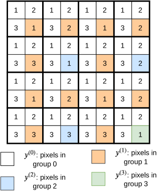
Figure 2: Pixel groups and subgroups when an $8\times 8$ latent representation $y$ is downsampled 3 times by a factor of 2. The color indicates the division of groups and the number in each block indicates the subgroup index that the pixel belongs to. $2\times 2$ subgroup blocks are marked with thicker borders.

Next, we assume that the pixels in each subgroup are mutually independent on the condition of their context. Let $y_{(k)}^{(i,j)}$ be the pixel $k$ in $y^{(i,j)}$ and $d$ be the total number of pixels in $y^{(i,j)}$. We have

$$p\left(y^{(i,j)}|C^{(i,j)}\right)=\prod_{k=1}^{d}p\left(y_{(k)}^{(i,j)}|C^{(i,j)}\right).$$ (10)

Eqs. 8, 9 and 10 defines a factored form of the variational distribution function $p\left(y\right)$. It can be seen that the PixelCNN is a special case of the MSP model when $s=0$, $b=n$ and subgroups are designed to be in a raster scan order.

In theory, we can downsample $y$ multiple times until there is 1 pixel in the last scale. [32] shows that there is only 0.4% of data at scale 4. Thus choosing $s$ to be $3$ or $4$ is enough in practice.

III-B Channel dependencies

Channel dependency is another important aspect to build a powerful variational distribution function [26, 9, 22, 27]. In [32], a full channel dependency mode is used in lossless image compression. However, when the number of channels increases, the complexity of the full channel model increases exponentially, which prevents it from being used in LIC systems. Next, we analyze the properties of the channels in the latent representation.

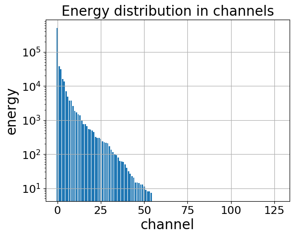
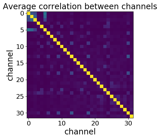
(a)	(b)

Figure 3: (a) Energy distribution of the channels in $y$. (b) Correlation between the first 32 channels sorted by their energy.

First, the energy distribution is heavily unbalanced in the channels. Figure 3 (a) shows the energy distribution of channels in $y$ on data collected from compressing Kodak dataset [33] using a LIC system without channel dependency exploitation. The first 32 channels account for 99.9% of the overall energy of the total 128 channels. The low energy channels are very sparse, for example, only 0.1% of the elements are non-zeros in the last 96 channels.

Next, unlike in the image domain where the channels are highly correlated, the correlation among the channels is low. Figure 3 (b) shows the average correlation between the top 32 channels. Only a few pairs of channels show a meaningful level of correlation among all the 32 channels.

Based on these observations, exploiting channel dependencies among a large number of channels is not necessary. we partition the channels into two groups. The first group, named as seed group, contains $a$ number of channels and the second group contains the rest of the channels. The channels in the seed group are processed in the full dependency mode while the channels in the second group are processed in parallel with dependency to the seed group. The full dependency mode for the seed group does not increase the complexity dramatically since $a$ is a small number. In our experiments, up to $4$ channels in the seed group are enough to capture the dependencies among the channels. Figure 4 shows the channel dependency modes of the proposed system and other LIC systems.

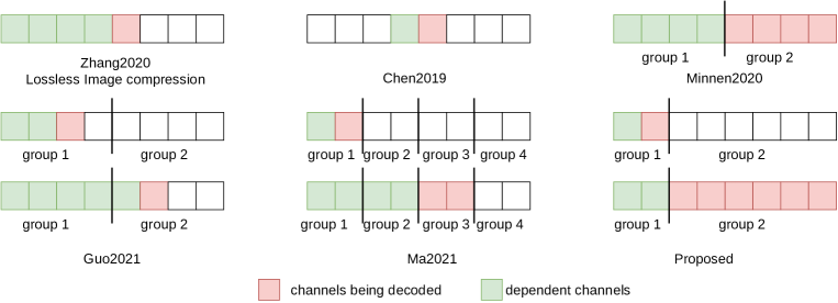
Figure 4: Channel dependency modes of different LIC systems

The probability distribution of pixel $y_{(k)}$ is

$$p\left(y_{(k)}\right)=\prod_{l=2}^{a}p\left(y_{(k,l)}|y_{(k,l-1)},\cdots,y_{(k,1)},C\right)$$ (11)

$$\quad p\left(y_{(k,1)}|C\right)\prod_{l=a+1}^{c}p\left(y_{(k,l)}|y_{(k,a)},\cdots y_{(k,1)},C\right)$$

where $y_{(k,l)}$ is the $l$-th channel element in pixel $k$, $c$ is the number of channels and $C$ is the context of pixel $k$. Note that, superscript $(i,j)$ is omitted in Eq. 11 for simplicity.

III-C MSP probability model architecture

As defined in Eqs. 8, 9, 10 and 11, we model the variational distribution $p\left(y\right)$ in a factorized form where the dependencies among the elements are sufficiently exploited. The elements in $y$ are divided into groups, subgroups, and channel groups. The elements in the same channel group are mutually independent on the condition of their context and are processed in parallel. The context of each channel group contains all the elements that are available.

At last, we assume that each element in $y$ follows a Gaussian distribution with parameter $\mu$ and $\sigma^{2}$ for the mean and variance, respectively. $\mu$ and $\sigma^{2}$ are determined by function $h_{p}(C)$, where $C$ is the context for the element. The cross-entropy loss defined in Eq. 4 is calculated by Eqs. 8, 9, 10 and 11 using the derived parameters for the Gaussian distribution functions.

Given the factorized form of the variational distribution function, the decoder takes $s\cdot b\cdot(a+1)+1$ steps to decode the latent representation from the bitstream. Since $s$, $b$ and $a$ are predefined constants, the decoding complexity of the proposed LIC system is $O(1)$.

To implement the grouped dependencies of the elements in $y$, we introduce a mixture tensor $\bar{y}$, as context $C$, that contains the true values of $y$ that are already available and the predicted values of $y$ that have not been available at the decoding stage. A binary tensor $m$ is used to indicate the true elements in $\bar{y}$. After a set of elements are processed, the corresponding elements in $\bar{y}$ are updated with the true values from $y$ and $m$ is also updated accordingly. A deep CNN, implementing $h_{p}\left(\bar{y},m\right)$, estimates the parameters of the Gaussian distribution for the elements to be processed.

For the last scale, $y^{(s)}$, since there is no context, we use the uni-variate non-parametric density model [18] for the probability distribution. This model has been proved to be effective in other LIC systems in modeling the hyperprior variables and the implementations are readily available in many software packages [19].

Algorithm 1 shows the operations of the MSP probability model when estimating the rate loss for $y$ at the training stage. Function $h_{s}\left(y^{(s)}\right)$ estimates the cross-entropy of $y^{(s)}$ using the non-parametric density model and function $h_{p}\left(\bar{y}^{(i)},m^{(i)}\right)$ outputs the estimated Gaussian parameters for elements in $y^{(i)}$. The architecture of the deep neural network implementing $h_{p}(\cdot)$ is shown in the appendix.

Algorithm 1 Estimating the rate loss at the training stage

given

latent representation $y$

generate

$n\sim U(-0.5,0.5)$

$y=y+n$

$y^{(0)},y^{(1)},\cdots,y^{(s)}\leftarrow downsample(y)\;\mathrm{(nearest\ neighbor\ downsampling)}$

$r=-\log_{2}h_{s}\left(y^{(s)}\right)\ \mathrm{(rate\ loss\ of\ the\ last\ scale)}$

for

each $i$ in scale $s-1,\cdots,0$

$\bar{y}^{(i)}=upsample\left(y^{(i+1)}\right)\ \mathrm{(nearest\ neighbor\ upsampling)}$

$m^{(i)}=zero\left(y^{(i)}\right)$

for

each $j$ in subgroup $1,\cdots,b$

for

each $l$ in channel $1,\cdots,a$

$\mu_{(k,l)}^{(i,j)},\sigma_{(k,l)}^{(i,j)}\leftarrow h_{p}\left(\bar{y}^{(i)},m^{(i)}\right),\ k=1,\cdots,d$

$r=r+\left[-\sum_{k}\log_{2}p\left(y_{(k,l)}^{(i,j)}|\mu_{(k,l)}^{(i,j)},\sigma_{(k,l)}^{(i,j)}\right)\right]$

$\bar{y}_{(k,l)}^{(i,j)}=y_{(k,l)}^{(i,j)},\ k=1,\cdots,d$

$m_{(k,l)}^{(i,j)}=1,\ k=1,\cdots,d$

$r=r+\left[-\sum_{k}\log_{2}p\left(y_{(k,a+1,\cdots,c)}^{(i,j)}|\hat{y}^{(i)},m^{(i)}\right)\right]$

return

$r$

III-D Latent representation overfitting

At the inference stage, i.e. encoding and decoding, the latent representation determines the size of the bitstream and the quality of the reconstructed image. A LIC system can use the input image as the ground truth to optimize the latent representation with the parameters of the decoder and the probability model fixed [34, 35]. This technique, known as latent representation overfitting (LOF), can efficiently improve the compression performance by mitigating the problem of domain shift [36], i.e., the characteristics of the input image significantly differing from the images in the training dataset. The loss function of LOF is defined as

$$L=-\log p(y)+\lambda d\left(x,g_{s}\left(y\right)\right),$$ (12)

and optimized with regard to $y$. Note that directly optimizing Eq. 12 is difficult since $y$ is a discrete tensor. Instead, we optimize the continuous latent representation $\tilde{y}$ and quantize $\tilde{y}$ to get $y$. The objective function can be written as

$$L=-\log p\left(Q\left(\tilde{y}\right)\right)+\lambda d\left(x,g_{s}\left(Q\left(\tilde{y}\right)\right)\right),$$ (13)

where $Q\left(\cdot\right)$ is the quantization operation.

Since the gradient of the quantization function is undefined on border values and zero elsewhere, a LIC system is normally trained by adding uniform noise (AUN) to approximate the quantization operation at inference time [37, 7]. However, the AUN method requires a large number of samples and iterations to converge. To optimize Eq. 13 efficiently, we opt for the straight-through estimation (STE) method [38] to help the training during the LOF. Since the gradients are normally small on a well-trained system, it may take many iterations to accumulate the updates to change the values in $y$ using normal training parameters. To solve this slow training problem, we apply a greedy search method which is different from common training practice. We start the optimization using a very large learning rate and record the best performing $\tilde{y}$ during the training. When the loss stops decreasing for a certain number of iterations, we rewind $\tilde{y}$ to the best performing state and continue the training with a lower learning rate. This procedure repeats until no improvement can be made. Pseudocode for this procedure is in the appendix.

IV Experiments

IV-A Profiles and training details

The MSP probability model used in our LIC system contains a number of parameters that affect the compression performance and the computational complexity. We define three profiles for the proposed LIC system. Table II shows the parameters for each profile and the number of steps for the LIC system to decode an image.

TABLE II: The profiles of the proposed LIC system used in the experiments. “None” in the channel seeds column means no channel dependency is exploited. The filter column shows the number of filters of the deep CNN used in the probability model.

profile	scales	subgroup block	channel seeds	filters	decoding steps
baseline	3	$2\times 2$	None	64	10
normal	3	$2\times 2$	2	64	28
extra	4	$2\times 4$	4	128	121

The proposed LIC systems with different profiles are trained using the Open Images dataset [39], which contains images collected from the Internet. The majority of the images in the Open Images dataset are compressed by JPEG [1]. The training and validation splits of the dataset are prepared in the same way as [31, 40, 41, 32]. The training split contains 340K images. The longest side of the training images is 1024 pixels. For each profile, 7 models are trained with different $\lambda$ values to achieve different compression rates. The details of training and evaluation are in the appendix.

IV-B Kodak results

Kodak dataset [33] is a popular dataset to benchmark the performance of image compression systems. The dataset contains 24 uncompressed images with the size of $768\times 512$ pixels. Table III shows the compression performance of various systems. In the table, “vtm” and “hm” are the reference implementations of the VVC/H.266 and the HEVC/H.265 standards, respectively. The BD-rate and BD-psnr are calculated using the VTM as the anchor. For the BD-rate, a lower value indicates a better compression performance. For BD-psnr, a higher value indicates a better performance. The numbers in the table, except those for our proposed systems, are reported by the CompressAI [19]. Note that encoding and decoding are performed on CPU for VTM and HM while on GPU for the LIC systems. Thus, the encoding and decoding time of the LIC systems are not directly comparable to the VTM and HM systems. Following the protocol defined in CompressAI, the encoding and decoding time of LIC systems do not consider the model loading and data preparation time. RD curves of the competing methods are in the appendix.

TABLE III: Compression performance on the Kodak dataset.

method	BD-rate	BD-psnr	Parameters	encoding time (s)	decoding time (s)
vtm [42]	0.00	0.00	-	125.87	0.13
hm [2]	23.31	-1.01	-	3.69	0.07
bmshj2018-hyperprior [18]	30.49	-1.26	5.08M	0.04	0.03
mbt2018 [11]	11.02	-0.49	14.13M	2.79	6.00
cheng2020-attn [8]	5.51	-0.23	13.18M	2.72	5.93
cheng2020-anchor [8]	3.68	-0.16	11.83M	2.75	5.94
ours: baseline	12.61	-0.56	5.71M	0.23	0.20
ours: normal	11.12	-0.50	5.79M	0.47	0.38
ours: extra	3.84	-0.18	7.85M	1.43	1.18
ours: baseline (LOF)	4.35	-0.20	5.71M	14.61	0.19
ours: normal (LOF)	3.44	-0.16	5.79M	31.88	0.38
ours: extra (LOF)	-2.54	0.12	7.85M	122.01	1.41

As Table III shows, the proposed LIC system with extra profile and LOF technique outperforms the competing systems, including VTM. Compared to other LIC systems, the proposed systems achieve similar or better performance with much smaller neural networks. Furthermore, the proposed systems can decode images much more efficiently than other LIC systems. Note that the difference between the baseline and the normal profile is channel dependency exploitation. The relatively small gain achieved by the normal profile indicates that the channels in the latent representation are not heavily correlated, as we studied in Section III-B.

Table III also shows significant gains that the LOF technique brings by sacrificing the encoding time. However, this is not a major issue for LIC systems since the encoding is normally done offline and once. The encoding and decoding operations in the traditional image and video codecs, such as VVC/H.266, are also asymmetric, i.e., the encoding is much more complicated than the decoding.

Figure 5 visualizes some selected reconstructed images from different systems on the Kodak dataset. For better visualization, two patches from each image are shown in higher resolution.

	uncompressed	VTM	Cheng2020-anchor	Extra	Extra (LOF)
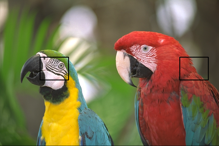
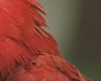
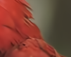
kodim23		0.238/37.37	0.235/37.59	0.229/37.25	0.220/37.57
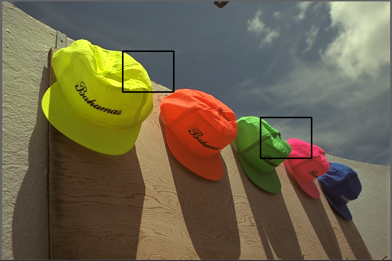
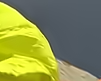
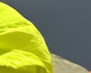
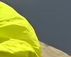
kodim03		0.114/33.72	0.128/33.94	0.118/33.82	0.109/33.96
kodim05		0.239/25.94	0.240/26.09	0.243/26.16	0.232/26.28

Figure 5: Visualized comparison of selected methods. The numbers below the patches are BPP/PSNR values.

IV-C CLIC2020 results

Next, we evaluate the performance of the proposed LIC systems using larger datasets. CLIC2020 dataset, divided into “mobile” and “professional” subsets, contains high-quality images. The average resolution of the images in the “mobile” and “professional” subset is $1913\times 1361$ and $1803\times 1175$, respectively. The test splits of the two subsets contain 178 and 250 images, respectively. Table IV shows the compression performance of the competing systems.

TABLE IV: Compression performance on the“mobile” and “professional” subset of the CLIC2020 dataset.

	“mobile” subset				“professional” subset
method	BD-rate	BD-psnr	encoding time (s)	decoding time (s)	BD-rate	BD-psnr	encoding time (s)	decoding time (s)
vtm [42]	0.00	0.00	688.93	0.78	0.00	0.00	1970.66	1.29
hm [2]	21.86	-0.96	24.63	0.46	26.56	-0.99	47.86	0.67
bmshj2018-hyperprior [18]	37.62	-1.41	0.27	0.17	44.67	-1.40	0.24	0.15
mbt2018 [11]	11.96	-0.50	21.53	45.99	11.03	-0.40	19.91	42.54
cheng2020-attn [8]	8.92	-0.35	21.10	45.15	5.97	-0.21	19.94	43.07
cheng2020-anchor [8]	8.29	-0.32	21.26	45.92	4.08	-0.14	19.84	42.76
ours: baseline	15.74	-0.69	0.68	0.64	21.27	-0.80	0.69	0.68
ours: normal	14.69	-0.64	0.92	0.80	20.92	-0.79	0.97	0.86
ours: extra	8.02	-0.36	2.76	2.20	11.72	-0.46	2.54	2.04
ours: baseline (LOF)	4.75	-0.21	70.00	0.61	6.06	-0.23	61.27	0.63
ours: normal (LOF)	4.12	-0.18	104.76	0.82	5.30	-0.20	102.29	0.85
ours: extra (LOF)	-1.04	0.04	423.46	2.18	-1.29	0.05	396.50	2.05

Similar to the results on the Kodak dataset, the proposed LIC system with extra profile and LOF technique outperforms other competing systems. It is important to note that the LIC systems using the PixelCNN type of context model are very inefficient in decoding large images. Compared to the values in Table III, the decoding time of these methods is proportional to the image size, which leads to over 40 seconds to decode one image. With the help of the MSP probability model, the decoding time of the proposed LIC system only increases slightly with a constant number compared to the results on the Kodak images. RD curves of the results on the CLIC2020 dataset are included in the appendix.

It can be noticed that the proposed methods perform better on the Kodak dataset than on the CLIC2020 dataset. Furthermore, the performance is better on the “mobile” subset than on the “professional” subset. This behavior may be caused by the training set we used to train our models. First, the training images are about the same size as the images in the Kodak dataset. Second, the quality of the training images, intended for computer vision tasks and heavily compressed using JPEG, are closer to the images in the “mobile” subset, while significantly different from the high-quality images in the “professional” subset.

Using the LOF technique, the BD-rate increases by 6.38, 9.33 and 13.01 on the Kodak dataset, “mobile” subset and “professional” subset, respectively. The significant gains demonstrate the effectiveness of the LOF technique in mitigating the domain shift problem.

V Discussions

Recent research on LIC systems have shown comparable or superior performance over the VVC/H.266 to some extent. For example, the Fu2021 [20] system has a similar performance as the VVC/H.266 at the bit rate less than 0.3 BPP and achieves 0.3 to 0.4 PSNR gain over the VVC/H.266 at the bit rate range [0.4, 0.9] BPP on the Kodak dataset. Ma2021 [22] system claims a BD-rate reduction of 2.5% at bit range [0.1, 0.9] BPP on the Kodak dataset, and 2.2% at bit range [0.05, 0.5] BPP on the “professional” subset of the CLIC2020 dataset. Guo2021 [9] LIC system claims a BD-rate reduction of 5.1% in bit rate range [0.15, 1] BPP on the Kodak dataset.

Section IV shows that the proposed LIC system achieves 2.54%, 1.04% and 1.29% BD-rate reduction on three benchmark datasets, respectively, compared to the VVC/H.266 over the bit rate range [0.04, 2] BPP. To our best knowledge, the proposed system is the first LIC system to achieve convincing BD-rate reduction over the VVC/H.266 on the full bit-rate range on these benchmark datasets.

More importantly, the proposed LIC system has a much lower decoding complexity compared to other LIC systems. The decoding complexity of Fu2021 is equal to or higher than the Cheng2020 system, which takes about 6 seconds to decode Kodak images and over 40 seconds to decode CLIC2020 images [8, 20]. Ma2021 system claims that the decoding time is 3.8 times of the Cheng2020 system [22]. The Guo2021 system takes about 38.7 seconds to decode Kodak images [9]. The decoding complexity of the proposed system is determined by the configuration constants. Experiments show that the proposed system is capable of decoding images up to 2K at about 2 seconds. However, it should be noted that the decoding time is also affected by the computational capacity of the hardware system. It takes about 5.5 seconds to decode a 4K image in our testing environment. We expect that this decoding time on large images can be greatly reduced in an environment with more computational capacity.

Experiment results also show that various balance points between compression efficiency and computational complexity can be easily accomplished by using predefined profiles. Some existing context models can be considered as special cases of the proposed framework. For example, the checkerboard context model defined in [17] is the MSP profile with 1 scale downsampling (in a checkerboard manner) and 1x1 subgroup block definition.

Although the LOF technique efficiently mitigates the domain-shift problem that our system encounters because of the low quality training images, we believe the performance of the proposed system can be further improved if the system is trained with a large number of uncompressed images.

We also trained the proposed system using MS-SSIM as the reconstruction loss in Eq. 3. The performance of the MS-SSIM trained systems is demonstrated in the appendix. Further studies about the impact of the profile parameters, such as scales $s$, subgroup size $b$ and seed group size $a$ are also included in the appendix.

VI Conclusion

In this paper, we proposed a novel LIC framework using an improved MSP probability model and the latent representation overfitting technique. The proposed system not only outperforms other LIC systems but also the state-of-the-art codec VVC/H.266, which is based on traditional technologies, on all three benchmark datasets over a wide bit rate range. More importantly, the proposed system improves the decoding complexity of previous LIC systems from $O(n)$ to $O(1)$, such that the decoding time for 2K images are reduced by more than 20 times. We also showed that the LOF technique efficiently mitigates the domain-shift problem of a LIC system. The compression performance of the proposed system can be further improved by various techniques and training setups, which will be further studied in the future.

References

- [1] JPEG, “Jpeg - jpeg 2000,” https://jpeg.org/jpeg2000/, 2022.
- [2] G. J. Sullivan, J.-R. Ohm, W.-J. Han, and T. Wiegand, “Overview of the high efficiency video coding (HEVC) standard,” IEEE Transactions on circuits and systems for video technology, vol. 22, no. 12, pp. 1649–1668, 2012, publisher: IEEE.
- [3] I. O. f. Standardization, “ISO/IEC 23090-3:2021 - Information technology — Coded representation of immersive media — Part 3: Versatile video coding,” 2021.
- [4] Y. Hu, W. Yang, Z. Ma, and J. Liu, “Learning End-to-End Lossy Image Compression: A Benchmark,” arXiv:2002.03711 [cs, eess], Mar. 2021, arXiv: 2002.03711. [Online]. Available: http://arxiv.org/abs/2002.03711
- [5] D. Marpe, T. Wiegand, and G. Sullivan, “The H.264/MPEG4 advanced video coding standard and its applications,” IEEE Communications Magazine, vol. 44, no. 8, pp. 134–143, Aug. 2006, conference Name: IEEE Communications Magazine.
- [6] T. K. Tan, R. Weerakkody, M. Mrak, N. Ramzan, V. Baroncini, J.-R. Ohm, and G. J. Sullivan, “Video quality evaluation methodology and verification testing of HEVC compression performance,” IEEE Transactions on Circuits and Systems for Video Technology, vol. 26, no. 1, pp. 76–90, 2015, publisher: IEEE.
- [7] J. Ballé, V. Laparra, and E. P. Simoncelli, “End-to-end Optimized Image Compression,” arXiv:1611.01704 [cs, math], Mar. 2017, arXiv: 1611.01704. [Online]. Available: http://arxiv.org/abs/1611.01704
- [8] Z. Cheng, H. Sun, M. Takeuchi, and J. Katto, “Learned Image Compression with Discretized Gaussian Mixture Likelihoods and Attention Modules,” arXiv:2001.01568 [eess], Mar. 2020, arXiv: 2001.01568. [Online]. Available: http://arxiv.org/abs/2001.01568
- [9] Z. Guo, Z. Zhang, R. Feng, and Z. Chen, “Causal Contextual Prediction for Learned Image Compression,” IEEE Transactions on Circuits and Systems for Video Technology, pp. 1–1, 2021, arXiv: 2011.09704. [Online]. Available: http://arxiv.org/abs/2011.09704
- [10] Y. Hu, W. Yang, and J. Liu, “Coarse-to-Fine Hyper-Prior Modeling for Learned Image Compression,” in AAAI Conference on Artificial Intelligenc, 2020.
- [11] D. Minnen, J. Ballé, and G. Toderici, “Joint Autoregressive and Hierarchical Priors for Learned Image Compression,” arXiv:1809.02736 [cs], Sep. 2018, arXiv: 1809.02736. [Online]. Available: http://arxiv.org/abs/1809.02736
- [12] L. Theis, W. Shi, A. Cunningham, and F. Huszár, “Lossy Image Compression with Compressive Autoencoders,” arXiv:1703.00395 [cs, stat], Mar. 2017, arXiv: 1703.00395. [Online]. Available: http://arxiv.org/abs/1703.00395
- [13] Y. Choi, M. El-Khamy, and J. Lee, “Variable Rate Deep Image Compression With a Conditional Autoencoder,” arXiv:1909.04802 [cs, eess], Sep. 2019, arXiv: 1909.04802. [Online]. Available: http://arxiv.org/abs/1909.04802
- [14] Y. Patel, S. Appalaraju, and R. Manmatha, “Human Perceptual Evaluations for Image Compression,” arXiv:1908.04187 [cs, eess], Aug. 2019, arXiv: 1908.04187. [Online]. Available: http://arxiv.org/abs/1908.04187
- [15] F. Mentzer, E. Agustsson, M. Tschannen, R. Timofte, and L. Van Gool, “Conditional Probability Models for Deep Image Compression,” arXiv:1801.04260 [cs], Jun. 2019, arXiv: 1801.04260. [Online]. Available: http://arxiv.org/abs/1801.04260
- [16] J. Zhao, B. Li, J. Li, R. Xiong, and Y. Lu, “A Universal Encoder Rate Distortion Optimization Framework for Learned Compression,” in 2021 IEEE/CVF Conference on Computer Vision and Pattern Recognition Workshops (CVPRW), Jun. 2021, pp. 1880–1884, iSSN: 2160-7516.
- [17] D. He, Y. Zheng, B. Sun, Y. Wang, and H. Qin, “Checkerboard Context Model for Efficient Learned Image Compression,” in 2021 IEEE/CVF Conference on Computer Vision and Pattern Recognition (CVPR), Jun. 2021. [Online]. Available: https://ieeexplore.ieee.org/document/9577406/
- [18] J. Ballé, D. Minnen, S. Singh, S. J. Hwang, and N. Johnston, “Variational image compression with a scale hyperprior,” arXiv:1802.01436 [cs, eess, math], May 2018, arXiv: 1802.01436. [Online]. Available: http://arxiv.org/abs/1802.01436
- [19] J. Bégaint, F. Racapé, S. Feltman, and A. Pushparaja, “CompressAI: a PyTorch library and evaluation platform for end-to-end compression research,” arXiv preprint arXiv:2011.03029, 2020.
- [20] H. Fu, F. Liang, J. Lin, B. Li, M. Akbari, J. Liang, G. Zhang, D. Liu, C. Tu, and J. Han, “Learned Image Compression with Discretized Gaussian-Laplacian-Logistic Mixture Model and Concatenated Residual Modules,” arXiv:2107.06463 [cs, eess], Jul. 2021, arXiv: 2107.06463. [Online]. Available: http://arxiv.org/abs/2107.06463
- [21] G. Gao, P. You, R. Pan, S. Han, Y. Zhang, Y. Dai, and H. Lee, “Neural Image Compression via Attentional Multi-Scale Back Projection and Frequency Decomposition,” in Proceedings of the IEEE/CVF International Conference on Computer Vision (ICCV), Oct. 2021, pp. 14 677–14 686.
- [22] C. Ma, Z. Wang, R. Liao, and Y. Ye, “A Cross Channel Context Model for Latents in Deep Image Compression,” arXiv:2103.02884 [cs, eess], Mar. 2021, arXiv: 2103.02884. [Online]. Available: http://arxiv.org/abs/2103.02884
- [23] Y. Xie, K. L. Cheng, and Q. Chen, “Enhanced invertible encoding for learned image compression,” arXiv preprint arXiv:2108.03690, 2021.
- [24] D. He, Y. Zheng, B. Sun, Y. Wang, and H. Qin, “Checkerboard Context Model for Efficient Learned Image Compression,” arXiv:2103.15306 [cs, eess], Apr. 2021, arXiv: 2103.15306. [Online]. Available: http://arxiv.org/abs/2103.15306
- [25] Z. Wang, E. Simoncelli, and A. Bovik, “Multiscale structural similarity for image quality assessment,” in The Thrity-Seventh Asilomar Conference on Signals, Systems Computers, 2003, vol. 2, Nov. 2003, pp. 1398–1402 Vol.2.
- [26] T. Chen, H. Liu, Z. Ma, Q. Shen, X. Cao, and Y. Wang, “Neural Image Compression via Non-Local Attention Optimization and Improved Context Modeling,” arXiv:1910.06244 [eess], Oct. 2019, arXiv: 1910.06244. [Online]. Available: http://arxiv.org/abs/1910.06244
- [27] D. Minnen and S. Singh, “Channel-wise Autoregressive Entropy Models for Learned Image Compression,” arXiv:2007.08739 [cs, eess, math], Jul. 2020, arXiv: 2007.08739. [Online]. Available: http://arxiv.org/abs/2007.08739
- [28] A. Jain, P. Abbeel, and D. Pathak, “Locally masked convolution for autoregressive models,” arXiv:2006.12486 [cs, stat], Jun 2020. [Online]. Available: http://arxiv.org/abs/2006.12486
- [29] A. v. d. Oord, N. Kalchbrenner, O. Vinyals, L. Espeholt, A. Graves, and K. Kavukcuoglu, “Conditional Image Generation with PixelCNN Decoders,” arXiv:1606.05328 [cs], Jun. 2016, arXiv: 1606.05328. [Online]. Available: http://arxiv.org/abs/1606.05328
- [30] T. Salimans, A. Karpathy, X. Chen, and D. P. Kingma, “PixelCNN++: Improving the PixelCNN with Discretized Logistic Mixture Likelihood and Other Modifications,” Nov. 2016. [Online]. Available: https://openreview.net/forum?id=BJrFC6ceg
- [31] S. Cao, C.-Y. Wu, and P. Krähenbühl, “Lossless Image Compression through Super-Resolution,” arXiv:2004.02872 [cs, eess], Apr. 2020, arXiv: 2004.02872. [Online]. Available: http://arxiv.org/abs/2004.02872
- [32] H. Zhang, F. Cricri, H. R. Tavakoli, N. Zou, E. Aksu, and M. M. Hannuksela, “Lossless Image Compression Using a Multi-Scale Progressive Statistical Model,” in Proceedings of the Asian Conference on Computer Vision (ACCV), Nov. 2020.
- [33] Kodak, “True Color Kodak Images,” 2022. [Online]. Available: http://r0k.us/graphics/kodak/
- [34] J. Campos, S. Meierhans, A. Djelouah, and C. Schroers, “Content Adaptive Optimization for Neural Image Compression,” arXiv:1906.01223 [cs, eess], Jun. 2019, arXiv: 1906.01223. [Online]. Available: http://arxiv.org/abs/1906.01223
- [35] N. Zou, H. Zhang, F. Cricri, H. R. Tavakoli, J. Lainema, M. Hannuksela, E. Aksu, and E. Rahtu, “L2C – Learning to Learn to Compress,” Proceedings of the IEEE 22nd International Workshop on Multimedia Signal Processing (MMSP), Jul. 2020, arXiv: 2007.16054. [Online]. Available: http://arxiv.org/abs/2007.16054
- [36] D. Krueger, E. Caballero, J.-H. Jacobsen, A. Zhang, J. Binas, D. Zhang, R. L. Priol, and A. Courville, “Out-of-Distribution Generalization via Risk Extrapolation (REx),” arXiv:2003.00688 [cs, stat], Feb. 2021, arXiv: 2003.00688. [Online]. Available: http://arxiv.org/abs/2003.00688
- [37] E. Agustsson and L. Theis, “Universally Quantized Neural Compression,” arXiv:2006.09952 [cs, math, stat], Oct. 2020, arXiv: 2006.09952. [Online]. Available: http://arxiv.org/abs/2006.09952
- [38] Y. Bengio, N. Léonard, and A. Courville, “Estimating or Propagating Gradients Through Stochastic Neurons for Conditional Computation,” arXiv:1308.3432 [cs], Aug. 2013, arXiv: 1308.3432. [Online]. Available: http://arxiv.org/abs/1308.3432
- [39] A. Kuznetsova, H. Rom, N. Alldrin, J. Uijlings, I. Krasin, J. Pont-Tuset, S. Kamali, S. Popov, M. Malloci, A. Kolesnikov, T. Duerig, and V. Ferrari, “The Open Images Dataset V4: Unified image classification, object detection, and visual relationship detection at scale,” IJCV, 2020.
- [40] F. Mentzer, E. Agustsson, M. Tschannen, R. Timofte, and L. Van Gool, “Practical Full Resolution Learned Lossless Image Compression,” arXiv:1811.12817 [cs, eess], May 2019, arXiv: 1811.12817. [Online]. Available: http://arxiv.org/abs/1811.12817
- [41] F. Mentzer, L. Van Gool, and M. Tschannen, “Learning Better Lossless Compression Using Lossy Compression,” arXiv:2003.10184 [cs, eess], Mar. 2020, arXiv: 2003.10184. [Online]. Available: http://arxiv.org/abs/2003.10184
- [42] B. Bross, J. Chen, S. Liu, and Y.-K. Wang, “Versatile Video Coding (Draft 8),” Joint Video Experts Team (JVET), Document JVET-Q2001, Jan. 2020.