Developable Quad Meshes and Contact Element Nets

Abstract.

The property of a surface being developable can be expressed in different equivalent ways, by vanishing Gauss curvature, or by the existence of isometric mappings to planar domains. Computational contributions to this topic range from special parametrizations to discrete-isometric mappings. However, so far a local criterion expressing developability of general quad meshes has been lacking. In this paper, we propose a new and efficient discrete developability criterion that is applied to quad meshes equipped with vertex weights, and which is motivated by a well-known characterization in differential geometry, namely a rank-deficient second fundamental form. We assign contact elements to the faces of meshes and ruling vectors to the edges, which in combination yield a developability condition per face. Using standard optimization procedures, we are able to perform interactive design and developable lofting. The meshes we employ are combinatorially regular quad meshes with isolated singularities but are otherwise not required to follow any special curves on a developable surface. They are thus easily embedded into a design workflow involving standard operations like remeshing, trimming, and merging operations. An important feature is that we can directly derive a watertight, rational bi-quadratic spline surface from our meshes. Remarkably, it occurs as the limit of weighted Doo-Sabin subdivision, which acts in an interpolatory manner on contact elements.

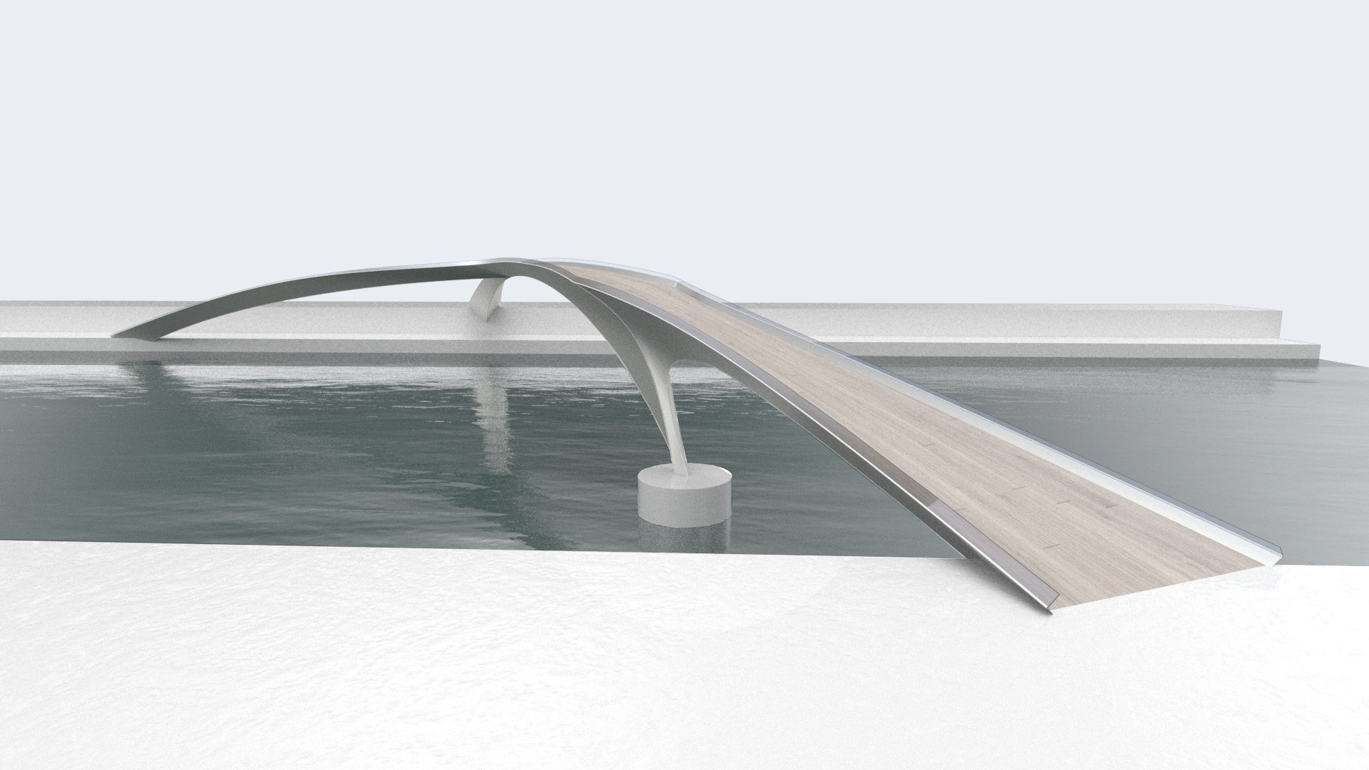
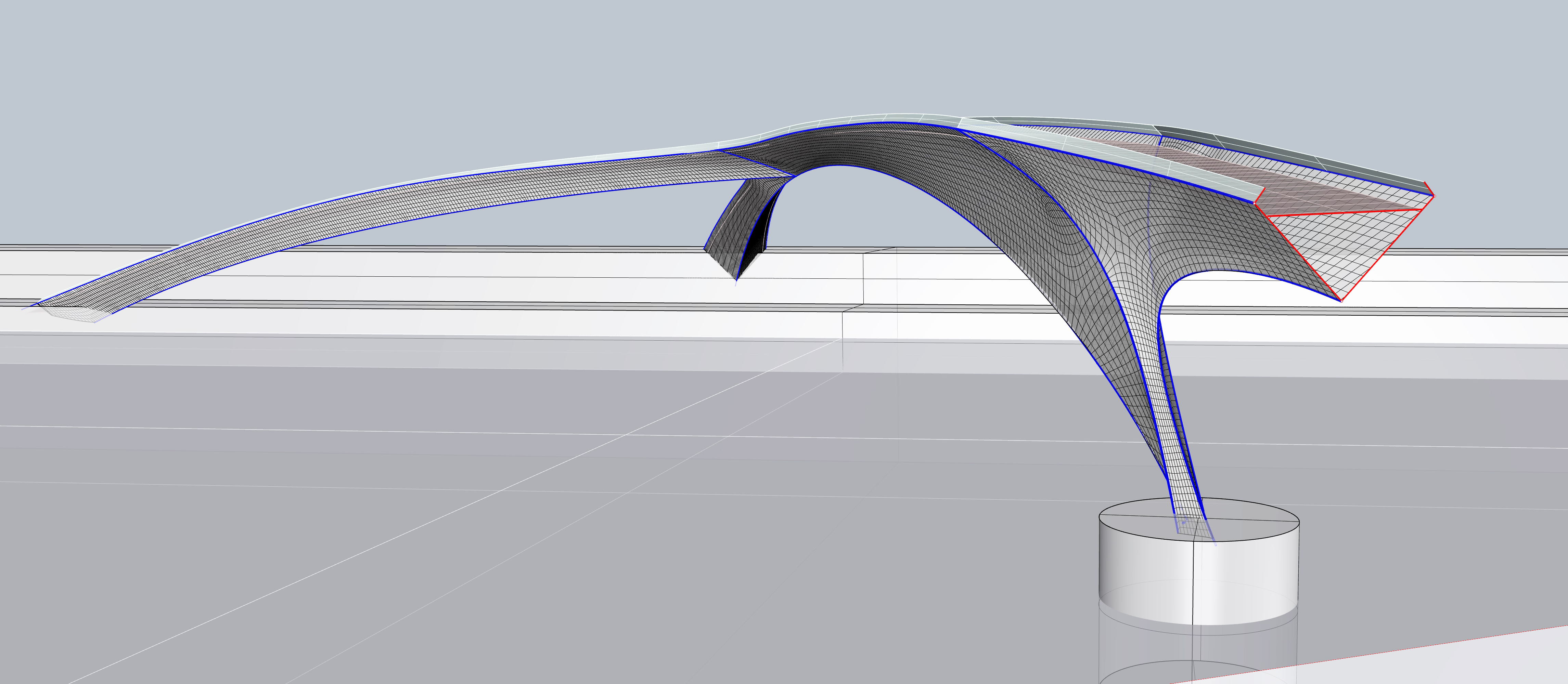
6mm 5mm 5mm 2mm 70mm 12mm 9mm 3mm 26mm 10mm 20mm 7mm

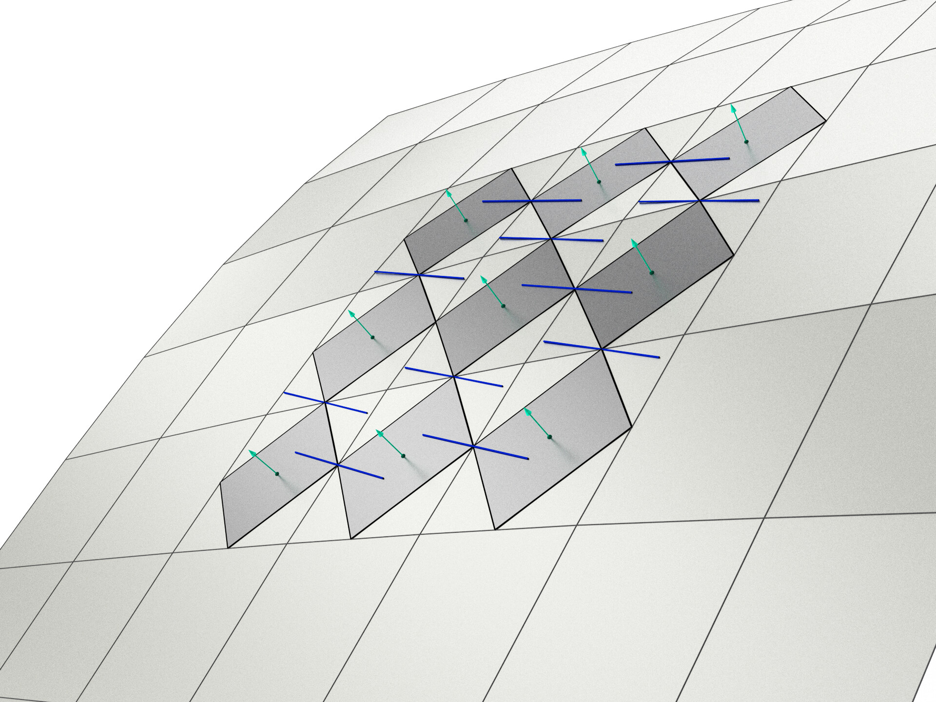
Figure 1. An architectural design based on challenging developable lofting tasks. CAD software has been used to connect given boundaries by a NURBS loft, followed by quad remeshing. Subsequently, our optimization towards developability has been applied. Observe that patches have several boundaries, and meshes exhibit combinatorial singularities. From left to right, we show the resulting design, meshes representing developables, and a zoomed-in detail revealing a discrete-developable quad mesh, endowed with inscribed contact elements, and the ruling line field we get from intersecting neighboring contact elements.

1. Introduction

The numerical and geometric modeling of developable surfaces has attracted attention for many years, starting with the first mesh representations proposed by R. Sauer (1970). One reason for that is the great practical importance of developables, which represent shapes made by bending flat pieces of inextensible sheet material. New algorithms continue to emerge, as do new applications — we only point to the construction of metamaterials that can be speedily laser-cut and fill volumes in the manner of ruffles by Signer et al. (2021), and the use of developables in interactive physical book simulation by Wolf et al. (2021).

A developable surface is unanimously defined by the existence of local isometric mappings to planar domains. As it turns out, the physical reality of bending thin sheets is modeled by surfaces exhibiting piecewise $C^{2}$ smoothness, which means surfaces exhibiting curvature continuity except for creases along curves. Geometric modeling of developables has been confined to this case. The continuous new proposals for the computational treatment of developables are a sign that the problem has not yet been satisfactorily solved. Another reason is the mathematical complexity of the subject itself, as well as the fact that $C^{2}$ developables enjoy many different but equivalent characterizations. These include vanishing Gauss curvature or other equivalent infinitesimal properties; line contact with tangent planes; or the existence of a local planar development. Each of these properties has been the basis of a computational approach, and each serves as motivation for defining a certain kind of discrete developable surface. This is also true for the present paper: We use the fact that developability is characterized by a rank deficient second fundamental form, and we employ the checkerboard patterns proposed by Peng et al. (2019) to express this in a discrete way. The basic entity we work with is a contact element, which is a weighted point plus a normal vector.

1.1. Overview and Contributions

$\bullet$  We present a new quad-mesh-based discrete model of developable surfaces which does not require the use of a development. Neither do edges have to be aligned with special curves on the surface under consideration. It is based on so-called contact elements inscribed in the faces of the mesh which are defined via vertex weights (§ 2.2).

$\bullet$  The contact element net derived from a quad mesh is used to express discrete developability (§ 2.3), and also to derive a watertight spline surface interpolating contact elements. Incidentally that spline surface is the limit of weighted Doo-Sabin subdivision which acts in an interpolatory manner on contact elements (§ 2.2.2).

$\bullet$  The discrete developability property is achieved by optimization, essentially performing a projection onto the constraint manifold, guided by soft constraints like fairness and proximity to a reference surface (§ 2.4). When needed, we can combine our method with the isometric mappings proposed by Jiang et al. (2020).

$\bullet$  Interactive design of developables can mean the isometric deformation of a given flat piece as well as generally modifying a design surface such that developability is maintained as a constraint. We are able to do both (§ 3).

$\bullet$  Modeling tools treated in this paper include developable lofting, which is an old problem not easily accessible with previous methods (§ 3.2). A user can interactively modify developables by pulling on handles and letting developables glide through guiding curves; attaching a developable patch to a surface; and positioning singular curves. The refinement property of contact element nets allows for a multiresolution approach to modeling developables (§ 3.3).

1.2. Previous Work

There is a large body of literature about geometric modeling of and with developable surfaces. Our brief overview is subdivided according to the way developables are represented, either as spline surfaces or as discrete surfaces.

1.2.1. Previous work based on splines

It is known that developables consist of ruled surfaces enjoying torsality, i.e., the tangent plane along a ruling is constant. A ruled surface can be modeled as a degree $(1,n)$ B-spline surface — one family of parameter lines then will be the surface’s rulings. Torsality is a nonlinear constraint (Lang and Röschel, 1992) that can be achieved by optimization (Tang et al., 2016; Jiang et al., 2019). One limitation of such a method is the necessity to decompose developables into ruled pieces. The method thus may not be suitable for modeling deformations of developables where that decomposition may change.

A torsal ruled surface is the envelope of its tangent planes, and thus essentially is a curve in the dual space of planes. This fact has been exploited by Bodduluri and Ravani (1993) and follow-up publications. It reduces the design of ruled developables to the design of curves. The drawback of this method is that, in addition to the one mentioned in the previous paragraph, working in plane space is not intuitive and does not naturally avoid singularities.

Finally, we point to Jiang et al. (2020) who impose approximate developability on spline surfaces via conversion to a quad mesh. Here rulings do not have to coincide with parameter lines, cf. § 1.2.2.

1.2.2. Previous work based on quad meshes

The textbook (Sauer, 1970) proposes discrete developables based on the fact that developables are the envelopes of their tangent planes: A discrete ruled developable is simply a sequence of flat quads, and the edges between them play the role of rulings. This property lies on the basis of quad-meshing of developables, see recent work by Verhoeven at al. (2022). Such ruling-based developables are the basis of work by Liu et al. (2006) and Solomon et al. (2012). Their disadvantages are the same as for other ruling-based methods: it is difficult to model situations where the ruling pattern of a developable changes.

A different characterization of developables, the existence of a network of orthogonal geodesics, is the basis of work by Rabinovich et al. (2018a; 2018b; 2019) and Ion et al. (2020). Here developables are represented by quad meshes whose edges are not necessarily aligned with the rulings, but nevertheless are in a special position — they discretize a network of orthogonally intersecting geodesics.

Jiang et al. (2020) use discrete-isometric mappings to handle developables: A surface is represented by a quad mesh whose edges do not have any special relation to the surface. Developability is imposed by maintaining a second mesh in ${\mathbb{R}}\!^{2}$ isometric to the first mesh. Similarly, the work by Chern et al. (2018) is also capable of handling developables via isometric mappings to planar domains.

1.2.3. Previous work based on other discretizations

A triangle mesh is intrinsically flat except at the vertices, and it is in fact locally flat if and only if the angle sum in its vertices equals $2\pi$. This natural discretization of the concept of a developable surface has not been in much use in geometric modeling. An exception is provided by meshes consisting of equilateral triangles as used by Jiang et at. (2015). Better suited for geometric design of developables is the ‘local hinge’ condition imposed by Stein et al. (2018). It ensures the existence of rulings and also implies that the position of edges is not arbitrary; every face has an edge that represents the direction of a ruling. Binninger et al. (2021) approximate surfaces with piecewise-developable ones by thinning the Gauss image; their method operates on a triangle mesh.

Sellán et al. (2020) use an entirely different way of imposing developability. A height field $z=f(x,y)$ represents a developable surface if and only if the Hessian of $f$ has a vanishing determinant. A certain convex optimization converts a given height field to one where the Hessian is nonsingular only along 1D curves. This leads to a piecewise-developable surface. Our method is also based on the characterization of developables as surfaces with low-rank second fundamental forms. Our discretization, however, works for any quad mesh, and is not limited to height fields.

1.2.4. Previous work on Contact Elements

In the continuous setting, contact elements have been used in differential geometry and analysis since the 19th century. In the discrete setting, contact elements are implicitly present every time vertices are treated together with normal vectors. There are only a few contributions explicitly based on contact elements, such as the discrete principal meshes proposed by Bobenko and Suris (2007) and subsequent treatment of a discrete curvature theory and related topics (Schröcker, 2010; Bobenko et al., 2010; Rörig and Szewieczek, 2021).

2. Discrete Developables

2.1. Differential Geometry of Smooth Developables

We consider surfaces that are piecewise curvature continuous and which enjoy the property of being locally isometric to a planar domain. It is well known (see e.g. (Guggenheimer, 1963)) that this intrinsic flatness is characterized by the vanishing of Gauss curvature, $K=0$. It is also well known that one family of principal curvature lines of such surfaces is composed of straight lines, and that the tangent plane along these straight lines (rulings) is constant. The rulings extend all the way to the boundary of the surface. A developable thus decomposes into ruled surface pieces and planar parts. In geometric modeling, the number of pieces is assumed to be finite. We also consider surfaces consisting of individual developable pieces.

Gauss Image and 2nd Fundamental Form

The Gauss image of a developable is the set of its unit normal vectors. It is contained in the unit sphere $S^{2}$, and it decomposes into curves, one for each ruled piece.

In each point $p$ of the surface, the second fundamental form ${\mathord{\rm II}}_{p}({\text{v}},{\text{w}})$ governs curvatures. It takes as arguments vectors ${\text{v}},{\text{w}}$ tangent to the surface. If ${\text{x}}(u,v)$ is a parametrization, and ${\text{n}}(u,v)$ is the corresponding unit normal vector field, then the second fundamental form relates their derivatives via

$${\mathord{\rm II}}_{p}({\text{x}}_{u},{\text{x}}_{u}) =\langle{\text{x}}_{u},-{\text{n}}_{u}\rangle,\quad{\mathord{\rm II}}_{p}({\text{x}}_{u},{\text{x}}_{v})=\langle{\text{x}}_{u},-{\text{n}}_{v}\rangle,$$

$${\mathord{\rm II}}_{p}({\text{x}}_{v},{\text{x}}_{v}) =\langle{\text{x}}_{v},-{\text{n}}_{v}\rangle.$$

By linearity, ${\mathord{\rm II}}$ is now defined for all tangent vectors.

Figure 2. A developable touching another surface along a curve ${\text{c}}(t)$. Its rulings $r(t)$ are conjugate to the derivative vectors $\dot{\text{c}}(t)$.
\begin{overpic}[width=260.17464pt]{figures/illustrations/strip} \color[rgb]{0.7,0.0,0.1}\put(40.0,40.0){\hbox to0.0pt{\hss{\contour{white}{$r(t)$}}\hss}} \color[rgb]{0,0,0.5}\put(37.0,23.0){\vbox to0.0pt{\hbox{{${\text{c}}(t)$}}\vss}} \put(20.0,24.0){\hbox to0.0pt{\hss{\vbox to0.0pt{\hbox{{$\dot{\text{c}}(t)$}}\vss}}\hss}} \end{overpic}

The Conjugacy Relation and Developability

Tangent vectors ${\text{v}},{\text{w}}$ attached to the same point $p$ are called conjugate, if

$${\mathord{\rm II}}_{p}({\text{v}},{\text{w}})=0.$$

Gauss curvature vanishes in $p$ if and only if ${\mathord{\rm II}}_{p}$ has rank less than $2$ and exhibits a kernel (the ruling) which is conjugate to all tangent vectors. This can equivalently be expressed by the existence of a tangent vector which obeys

(1) $${\mathord{\rm II}}({\text{x}}_{u},{\text{r}})={\mathord{\rm II}}({\text{x}}_{v},{\text{r}})=0\quad({\text{r}}\neq 0).$$

There is another property relating conjugacy of tangent vectors with developable surfaces: Suppose we have a curve ${\text{c}}(t)$ contained in a surface and a vector field ${\text{r}}(t)$ which is conjugate to the derivative $\dot{\text{c}}(t)$. Then the ruled surface ${\text{y}}(t,s)={\text{c}}(t)+s{\text{r}}(t)$ is tangent to the original surface along the curve c, and is itself developable (Liu et al., 2006). It is the envelope of the tangent planes of the surface along the curve c, and it is a geometric fact that the rulings of this envelope are conjugate to the tangents of the curve — see Fig. 2.

2.2. Contact Element Nets

It is our aim to express developability as a local property of a quad mesh whose edges and faces are allowed to be arbitrary. In contrast to previous work (Sauer, 1970; Liu et al., 2006) we do not require the faces to be planar, nor do we require the edges to be aligned with special curves on the surface, as is done by the previous references and by (Rabinovich et al., 2018b; Stein et al., 2018). We also do not need an isometric mapping to a planar domain.

2.2.1. Contact Element Nets From Weighted Vertices

We propose a developability condition that uses a generalized version of the checkerboard patterns approach used e.g. by (Jiang et al., 2020). For each edge they consider the midpoint, and for each face $f$, the inscribed parallelogram formed by those edge midpoints — see Fig. 3.

The center of the parallelogram together with a normal vector already form a contact element as it is. However, we aim for greater generality; we wish to consider not only parallelograms, but any planar quadrilateral inscribed in the faces of meshes.

Consider a quadrilateral, which needs not be planar, with vertices $v_{0},v_{1},v_{2},v_{3}$, and edge points $m_{e_{i}}$ on each edge $e_{i}=v_{i}v_{i+1}$ (indices modulo 4). The edge points shall not coincide with the vertices.

\begin{overpic}[width=212.47617pt]{figures/illustrations/face2} \put(0.0,60.0){${\mathbb{R}}\!^{4}$} \put(10.0,42.0){\hbox to0.0pt{\hss{$\widehat{v}_{0}$}}} \put(38.0,14.0){\hbox to0.0pt{\hss{\vbox to0.0pt{\hbox{$\widehat{v}_{1}$}\vss}}\hss}} \put(95.0,27.0){$\widehat{v}_{2}$} \put(62.0,64.0){$\widehat{v}_{3}$} \put(20.0,39.0){\hbox to0.0pt{\hss{\vbox to0.0pt{\vss\hbox{$\widehat{f}$}\vss}}\hss}}\put(35.0,37.0){\hbox to0.0pt{\hss{\vbox to0.0pt{\vss\hbox{$\widehat{\tau}_{f}$}\vss}}\hss}}\color[rgb]{0,0,0.5}\color[rgb]{0.7,0.0,0.1}\put(44.0,42.5){$\frac{\widehat{v}_{0}+\!\cdots+\widehat{v}_{3}}{4}$} \put(22.0,30.0){\hbox to0.0pt{\hss{\vbox to0.0pt{\hbox{$\frac{\widehat{v}_{0}+\widehat{v}_{1}}{2}$}\vss}}}} \put(65.0,17.0){\hbox to0.0pt{\hss{\vbox to0.0pt{\hbox{$\frac{\widehat{v}_{1}+\widehat{v}_{2}}{2}$}\vss}}\hss}} \end{overpic}

\begin{overpic}[width=212.47617pt]{figures/illustrations/face1} \put(0.0,60.0){${\mathbb{R}}\!^{3}$} \put(10.0,42.0){\hbox to0.0pt{\hss{$v_{0}$}}} \put(38.0,14.0){\hbox to0.0pt{\hss{\vbox to0.0pt{\hbox{$v_{1}$}\vss}}\hss}} \put(94.0,27.0){$v_{2}$} \put(62.0,64.0){$v_{3}$} \put(20.0,36.0){\hbox to0.0pt{\hss{\vbox to0.0pt{\vss\hbox{$f$}\vss}}\hss}}\put(37.0,35.0){\hbox to0.0pt{\hss{\vbox to0.0pt{\vss\hbox{$\tau_{f}$}\vss}}\hss}}\color[rgb]{0,0,0.5}\put(38.0,65.0){\hbox to0.0pt{\hss{${\text{n}}_{f}$}}} \color[rgb]{0.7,0.0,0.1}\put(52.0,42.0){$b_{f}$} \put(22.0,25.0){\hbox to0.0pt{\hss{$m_{e_{0}}$}}} \put(65.0,17.0){\hbox to0.0pt{\hss{\vbox to0.0pt{\hbox{$m_{e_{1}}$}\vss}}\hss}} \put(78.0,44.0){$m_{e_{2}}$} \put(35.0,56.0){\hbox to0.0pt{\hss{$m_{e_{3}}$}}} \end{overpic}

Figure 3. A contact element associated with the weighted vertices of a face $f$ is defined by points $m_{e_{i}}$ on the edges $e_{i}=v_{i}v_{i+1}$, the plane $\tau_{f}$ and its normal vector ${\text{n}}_{f}$, and the contact point $b_{f}$. The plane $\tau_{f}$ serves as a tangent plane associated with face $f$.

Lemma 2.1.

The edge points are co-planar if and only if the ratios of distances

$$(v_{i},m_{e_{i}},v_{i+1}):=\frac{\|m_{e_{i}}-v_{i}\|}{\|v_{i+1}-m_{e_{i}}\|}$$

fulfill the equation

(2) $$(v_{0},m_{e_{0}},v_{1})(v_{1},m_{e_{1}},v_{2})(v_{2},m_{e_{2}},v_{3})(v_{3},m_{e_{3}},v_{0})=1.$$

Proof.

Note that $(v_{i},m_{e_{i}},v_{i+1})$ equals the ratio of distances of points to any plane through $m_{e_{i}}$ not containing $v_{i},v_{i+1}$ Taking this plane as the one which spans 3 edge points, the product of ratios equals 1 if and only if the 4th point lies on the same plane, so that all distances in the product cancel out. ∎

The edge points can be described by weights $w_{i}>0$ associated with the vertices $v_{i}$ as

(3) $$m_{e_{i}} =\frac{1}{w_{i,i+1}}(w_{i}v_{i}+w_{i+1}v_{i+1}),\quad w_{i,j}=w_{i}+w_{j}.$$

Lemma 2.2.

Any choice of weights $w_{i}>0$ leads to co-planar edge points. Conversely, any co-planar edge points can be described by vertex weights.

Proof.

Given edge points as in Eq. (3), the ratios of distances become $(v_{i},m_{e_{i}},v_{i+1})=w_{i+1}/w_{i}$, so Eq. (2) holds. Conversely, to show the representation via weights, if Eq. (2) holds, we can obviously find weights $w_{i}>0$ to represent the points $m_{e_{i}}$. ∎

The setting of Lemma 2.2 is shown by Fig. 3. For any given quad mesh we therefore attach a weight to each vertex and define edge points on the edges by Eq. (3). It is convenient to represent weighted points in ${\mathbb{R}}\!^{3}$ by their homogeneous coordinates, letting

$$\widehat{v}_{i}=(w_{i}v_{i},w_{i})\in{\mathbb{R}}\!^{4}.$$

Given a weight $\lambda$, provided that $\lambda\neq 0$, any point $(x_{1},x_{2},x_{3},\lambda)\in{\mathbb{R}}\!^{4}$ corresponds to the point $(\frac{x_{1}}{\lambda},\frac{x_{2}}{\lambda},\frac{x_{3}}{\lambda})$ $\in$ ${\mathbb{R}}\!^{3}$. It is elementary that the edge points $m_{e_{i}}$ are represented by homogeneous coordinate vectors $\frac{1}{2}(\widehat{v}_{i}+\widehat{v}_{i+1})\equiv\widehat{v}_{i}+\widehat{v}_{i+1}$. This correspondence between vectors of ${\mathbb{R}}\!^{4}$ and points of ${\mathbb{R}}\!^{3}$ is illustrated by Fig. 3.

We think of the given quad mesh as approximating a smooth surface. For each face $f$, the plane containing the edge points represents a tangent plane $\tau_{f}$. Every face is thus naturally equipped with a unit normal vector ${\text{n}}_{f}$. It is natural to define the contact point $b_{f}$ as the weighted center of mass of vertices:

$$\widehat{b}_{f} =(\widehat{v}_{0}+\cdots+\widehat{v}_{3})/4\implies$$

$$b_{f} =(w_{0}v_{0}+\cdots+w_{3}v_{3})/w_{f},\quad w_{f}=w_{0}+w_{1}+w_{2}+w_{3}.$$

Here $w_{f}$ is a weight associated with the face $f$. It is easy to show that this contact point is the intersection of diagonals $m_{e_{0}}m_{e_{2}}$ and $m_{e_{1}}m_{e_{3}}$ — see Fig. 3. Note that we consider all unit normal vectors ${\text{n}}_{f}$ to be consistently oriented and pointing to one side of the mesh.

Lifting the mesh to ${\mathbb{R}}\!^{4}$ yields a checkerboard pattern in the original sense of (Jiang et al., 2020), where each face is equipped with an inscribed parallelogram (Fig. 3, left), defining a tangent plane $\widehat{\tau}_{f}$. The given quad mesh together with its edge points is a checkerboard pattern in ${\mathbb{R}}\!^{3}$ only if all vertex weights are equal.

\begin{overpic}[width=216.81pt]{figures/illustrations/doosabin2} \put(0.0,4.0){${\mathbb{R}}\!^{3}$}\color[rgb]{.7,.5,.2}\put(5.0,42.0){\hbox to0.0pt{\hss{$v_{0}$}}}\put(20.0,15.0){\hbox to0.0pt{\hss{\vbox to0.0pt{\hbox{$v_{1}$}\vss}}}}\put(55.0,28.0){\vbox to0.0pt{\hbox{\contour{white}{$v_{2}$}}\vss}}\put(33.0,45.0){\hbox to0.0pt{\hss{$v_{3}$}\hss}}\color[rgb]{0,0,0.5}\footnotesize\put(24.0,24.0){\hbox to0.0pt{\hss{\vbox to0.0pt{\hbox{$v_{1,f}^{\prime}$}\vss}}}}\put(16.0,34.0){\hbox to0.0pt{\hss{$v_{0,f}^{\prime}$}}}\color[rgb]{0.7,0.0,0.1}\put(31.0,54.0){\hbox to0.0pt{\hss{${\text{n}}_{f}$}}} \put(32.0,35.0){\hbox to0.0pt{\hss{\contour{white}{$b_{f}$}}}} \end{overpic}

\begin{overpic}[width=216.81pt]{figures/illustrations/doosabin3} \put(0.0,4.0){${\mathbb{R}}\!^{4}$}\color[rgb]{.7,.5,.2}\put(5.0,42.0){\hbox to0.0pt{\hss{$\widehat{v}_{0}$}}}\put(20.0,15.0){\hbox to0.0pt{\hss{\vbox to0.0pt{\hbox{$\widehat{v}_{1}$}\vss}}}}\put(33.0,45.0){\hbox to0.0pt{\hss{$\widehat{v}_{3}$}\hss}}\color[rgb]{0.7,0.0,0.1}\put(55.0,28.0){\vbox to0.0pt{\hbox{\contour{white}{$\widehat{v}_{2}$}}\vss}}\put(32.0,35.0){\hbox to0.0pt{\hss{\contour{white}{$\widehat{b}_{f}$}}}} \end{overpic}

Figure 4. Left: Doo-Sabin refinement acting on weighted vertices interpolates both the center $b_{f}$ of faces and the normal vectors ${\text{n}}_{f}$. Right: The limit surface of the subdivision is a biquadratic rational spline surface composed of rational Bézier patches. The control elements in ${\mathbb{R}}\!^{4}$ of the latter are derived from the homogeneous coordinates $\widehat{v}_{i}$ of vertices, from their midpoints $(\widehat{v}_{i}+\widehat{v}_{j})/2$, and from face midpoints, as shown in the figure.

2.2.2. Subdivision of Contact Element Nets

It is interesting that so-called dual quad-based subdivision rules are able to refine contact elements in a natural way, yielding a smooth limit surface. The well-known Doo-Sabin refinement rule even interpolates contact elements, as follows. We are going to apply it to homogeneous coordinate vectors $\widehat{v}_{i}\in{\mathbb{R}}\!^{4}$. For each vertex $\widehat{v}_{j}$ of a quadrilateral face $f=(v_{0}v_{1}v_{2}v_{3})$ we construct a new vertex

$$\widehat{v}_{j,f}^{\prime}=\frac{1}{16}(9\widehat{v}_{j}+3\widehat{v}_{j+1}+3\widehat{v}_{j-1}+\widehat{v}_{j+2})\quad\text{(indices mod 4)}.$$

In this way, each vertex, each edge, and also each face of the original mesh is naturally associated with a cycle of new vertices, yielding a new face each — see Fig. 4. For the refinement rule for $n$-gons with $n\neq 4$ we refer to (Peters and Reif, 2008).

For our purposes, the following observation is relevant: The center of mass $\widehat{f}=(\widehat{v}_{0}\widehat{v}_{1}\widehat{v}_{2}\widehat{v}_{3})$ of a face is invariant under subdivision:

$$\widehat{b}_{f}=\frac{1}{4}\sum\widehat{v}_{i,f}^{\prime}=\frac{1}{4}\sum\widehat{v}_{i}.$$

So are diagonals in inscribed quads, which span the tangent plane:

$$\frac{1}{2}\Big{(}\frac{1}{2}(\widehat{v}_{0}+\widehat{v}_{1})-\frac{1}{2}(\widehat{v}_{2}+\widehat{v}_{3})\Big{)}=\frac{1}{2}(\widehat{v}_{0,f}^{\prime}+\widehat{v}_{1,f}^{\prime})-\frac{1}{2}(\widehat{v}_{2,f}^{\prime}+\widehat{v}_{3,f}^{\prime}).$$

An illustration is provided by Fig. 4. Summing up, we get:

Proposition 2.3.

The Doo-Sabin refinement scheme, acting on the homogeneous coordinate representation of a regular quad mesh, interpolates contact elements. In the limit, it produces a $C^{1}$-smooth spline surface of the rational biquadratic type, whose spline control points are the weighted vertices we started from. That spline surface interpolates the contact elements of the original quad mesh.

The nature of the limit referred to in Prop. 2.3 is well known (Peters and Reif, 2008). If the original mesh is not a regular quad mesh, the statement remains true away from extraordinary points. Prop. 2.3 is relevant because it shows how to construct a smooth surface naturally connected to the data we work with. Note that Doo-Sabin subdivision surfaces in their simple form as shown here do not interpolate the boundary.

\begin{overpic}[width=346.89731pt]{figures/illustrations/sequence2a} \put(21.0,28.0){\hbox to0.0pt{\hss{\contour{white}{$m_{e_{0}}$}}\hss}} \put(41.0,32.0){\hbox to0.0pt{\hss{\contour{white}{$m_{e_{1}}$}}\hss}} \put(24.0,17.0){\hbox to0.0pt{\hss{\vbox to0.0pt{\hbox{$e_{0}$}\vss}}\hss}}\put(42.0,19.0){\hbox to0.0pt{\hss{\vbox to0.0pt{\hbox{$e_{1}$}\vss}}\hss}}\put(62.0,20.0){\hbox to0.0pt{\hss{\vbox to0.0pt{\hbox{$e_{2}$}\vss}}\hss}}\put(80.0,18.0){\hbox to0.0pt{\hss{\vbox to0.0pt{\hbox{$e_{3}$}\vss}}\hss}}\color[rgb]{0,0,0.5}\put(14.0,26.0){\hbox to0.0pt{\hss{\contour{white}{$b_{f_{0}}$}}}}\put(31.0,31.0){\hbox to0.0pt{\hss{\vbox to0.0pt{\vss\hbox{\contour{white}{$b_{f_{1}}$}}\vss}}\hss}}\color[rgb]{0.7,0.0,0.1}\put(25.0,36.0){\hbox to0.0pt{\hss{\contour{white}{$r_{e_{0}}$}}\hss}}\put(43.0,39.0){\hbox to0.0pt{\hss{\contour{white}{$r_{e_{1}}$}}\hss}}\put(63.0,40.0){\hbox to0.0pt{\hss{\contour{white}{$r_{e_{2}}$}}\hss}}\put(82.0,39.0){\hbox to0.0pt{\hss{\contour{white}{$r_{e_{3}}$}}\hss}}\end{overpic}

Figure 5. A discrete version of conjugacy. This discrete version of Fig. 2 shows a strip of contact elements comprised of faces $\{f_{i}\}$ with tangent planes $\{\tau_{f_{i}}\}$ and points of contact $\{b_{f_{i}}\}$. It represents a developable tangentially circumscribed to a surface along the discrete curve $\{b_{f_{i}}\}$. In analogy to the smooth case it is natural to define that discrete tangents $b_{f_{i+1}}-b_{f_{i}}$ and intersections $r_{e_{i}}=\tau_{f_{i}}\cap\tau_{f_{i+1}}$ are conjugate.

2.3. Developable Contact Element Nets

2.3.1. Conjugacy and Fields of Rulings

Consider a sequence of faces $f_{0},f_{1},\ldots$ which have common edges $f_{i}\cap f_{i+1}$ — see Fig. 5. Each is equipped with a tangent plane $\tau_{f_{i}}$. We now perform a construction that is a discrete analog of the envelope of tangent planes shown by Fig. 2: We construct the intersection lines of successive planes,

$$r_{e_{i}}=\tau_{f_{i}}\cap\tau_{f_{i+1}},\quad\text{where}\ e_{i}=f_{i}\cap f_{i+1}.$$

The line $r_{e_{i}}$ passes through the edge point $m_{e_{i}}$ as defined by Eq. (3). The line $r_{e_{i}}$ it is a discrete ruling of the discrete envelope of tangent planes along the discrete curve $b_{f_{0}},b_{f_{1}},\ldots$ (Sauer, 1970). In analogy to the smooth case shown, we postulate:

Definition 2.4.

The discrete envelope of tangent planes $\tau_{f_{0}},\tau_{f_{1}},\ldots$ along a discrete curve $b_{f_{0}},b_{f_{1}},\ldots$ is developable if discrete tangents $b_{f_{i+1}}-b_{f_{i}}$ and intersections $r_{e_{i}}=\tau_{f_{i}}\cap\tau_{f_{i+1}}$ are conjugate.

The direction of the ruling $r_{e_{i}}$ is indicated by a ruling vector associated with an oriented edge (half-edge) $\vec{e}_{i}$. If $\vec{e}_{i}$ and $-\vec{e}_{i}$ are the two half-edges corresponding to the edge $e_{i}=f_{i}\cap f_{i+1}$, we let

(4) $${\text{r}}_{\vec{e}_{i}}={\text{n}}_{f_{i}}\times{\text{n}}_{f_{i+1}}.$$

Here we assume that $f_{i}$ is to the left and $f_{i+1}$ to the right, and we also have ${\text{r}}_{-\vec{e}_{i}}=-{\text{r}}_{\vec{e}_{i}}$.

The vector ${\text{r}}_{\vec{e}_{i}}$ computed as a cross product in Eq. (4) is zero if neighbouring tangent planes $\tau_{f_{i}},\tau_{f_{i+1}}$ coincide. This happens e.g. if the mesh is flat, or the strip under consideration is flat.

Figure 7 shows what happens when we assign a ruling $r_{e}$ to all edges of a quad mesh. The rulings $r_{e}$ associated with the edges of a mesh are usually not samples of a continuous line field. However, in the case of a developable mesh, they indicate the kernel of the 2nd fundamental form, so they correspond to a single continuous line field.

\begin{overpic}[width=346.89731pt]{figures/illustrations/line_field} \end{overpic}

Figure 6. Left: On a general surface, the rulings associated with edges correspond to two distinct line fields (yellow and red). Right: Developability is characterized by the property that these line fields coincide.

Figure 7. Characterization of developability involving the ruling vectors ${\text{r}}_{\vec{e}_{0}},\ldots,{\text{r}}_{\vec{e}_{3}}$ associated with the cycle of edges around a face $f$.

\begin{overpic}[width=433.62pt]{figures/illustrations/vector_field} \color[rgb]{.7,.5,.2}\put(51.0,12.0){\hbox to0.0pt{\hss{\vbox to0.0pt{\hbox{\contour{white}{${\text{r}}_{\vec{e}_{0}}$}}\vss}}\hss}}\color[rgb]{.7,.5,.2}\put(68.0,74.0){\hbox to0.0pt{\hss{\contour{white}{${\text{r}}_{\vec{e}_{2}}$}}\hss}}\color[rgb]{0.7,0.0,0.1}\put(54.0,67.0){\hbox to0.0pt{\hss{\contour{white}{${\text{r}}_{\vec{e}_{3}}$}}\hss}}\color[rgb]{0.7,0.0,0.1}\put(63.0,20.0){\hbox to0.0pt{\hss{\vbox to0.0pt{\hbox{\contour{white}{${\text{r}}_{\vec{e}_{1}}$}}\vss}}\hss}}\end{overpic}

This way of computing rulings amounts to numerical differentiation. The definition of ruling vectors in Eq. (4) is valid provided a fair mesh that discretizes a smooth surface. We consider only such meshes where the edge polylines themselves are fair, so that they could be interpreted locally as a discrete version of the parameter lines of a $uv$ parametrization — which is no restriction.

2.3.2. Definition of Developable Quad Meshes

We express developability via the following property: A surface is developable if and only if its 2nd fundamental forms do not have full rank (do Carmo, 1976, p. 194). For a discrete version of this statement, it is useful to associate part of a 2nd fundamental form with each face of a mesh.

Consider a face $f=v_{0}v_{1}v_{2}v_{3}$ with its boundary cycle $\vec{e}_{0},\dots,\vec{e}_{3}$, assuming $e_{i}=f\cap f_{i}$. We define edge vectors ${\text{e}}_{i}=v_{i+1}-v_{i}$ (indices modulo $4$). We use Eq. (4) to compute ruling vectors ${\text{r}}_{\vec{e}_{0}},\ldots,{\text{r}}_{\vec{e}_{3}}$:

$${\text{r}}_{\vec{e}_{i}}={\text{n}}_{f}\times{\text{n}}_{f_{i}}.$$

Figure 7 shows this configuration. Note that the ruling vectors associated with opposite edges point in the opposite direction, like the edge vectors themselves.

We now partly define the matrix ${\mathord{\rm II}}_{f}$ of a 2nd fundamental form attached to the face center $b_{f}$. ${\mathord{\rm II}}_{f}$ governs conjugacy, and in fact Def. 2.4 already states such a conjugacy relation per edge. In order to formulate a conjugacy condition per face, we define average edge vectors

(5) $${\text{e}}_{02} =m_{e_{2}}-m_{e_{0}}=\frac{1}{w_{e_{2}}}(w_{2}v_{2}+w_{3}v_{3})-\frac{1}{w_{e_{0}}}(w_{1}v_{1}+w_{0}v_{0})$$

$${\text{e}}_{13} =m_{e_{3}}-m_{e_{1}}=\frac{1}{w_{e_{3}}}(w_{0}v_{0}+w_{3}v_{3})-\frac{1}{w_{e_{1}}}(w_{2}v_{2}+w_{1}v_{1}),$$

and we postulate that these average edge vectors are conjugate to average ruling vectors

$${\text{r}}_{\vec{e}_{13}}=\frac{1}{w_{f}}\Big{(}w_{e_{1}}{\text{r}}_{\vec{e}_{1}}+w_{e_{3}}(-{\text{r}}_{\vec{e}_{3}})\Big{)}\quad{\text{r}}_{\vec{e}_{02}}=\frac{1}{w_{f}}\Big{(}w_{e_{0}}{\text{r}}_{\vec{e}_{0}}+w_{e_{2}}(-{\text{r}}_{\vec{e}_{2}})\Big{)}.$$

The bilinear conjugacy relation per face then reads

(6) $${\text{e}}_{13}^{T}\cdot{\mathord{\rm II}}_{f}\cdot{\text{r}}_{\vec{e}_{13}}={\text{e}}_{02}^{T}\cdot{\mathord{\rm II}}_{f}\cdot{\text{r}}_{\vec{e}_{02}}=0,$$

where ${\mathord{\rm II}}_{f}$ is the symmetric $2\times 2$ matrix of a discrete second fundamental form associated with the face $f$. Equations (6) determine ${\mathord{\rm II}}_{f}$ uniquely up to a factor.

We now propose a definition of developability of quad meshes which uses the notions introduced above and discretizes several properties of smooth developables simultaneously:

Definition 2.5.

A quad mesh is developable if for all faces the average ruling vectors are parallel, i.e.,

(7) $${\text{r}}_{\vec{e}_{13}}\times{\text{r}}_{\vec{e}_{02}}=0.$$

This expresses the fact that each face is equipped with a single ruling direction, where rulings arise as intersections of neighboring tangent planes. Further, Eq. (7) implies that the conjugacy relation (6) is degenerate, because now two different average edge vectors are conjugate to the same ruling direction. It follows that

$$\det({\mathord{\rm II}}_{f})=0.$$

A further equivalent condition is $\det({\text{r}}_{\vec{e}_{13}},{\text{r}}_{\vec{e}_{02}},{\text{n}}_{f})=0$.

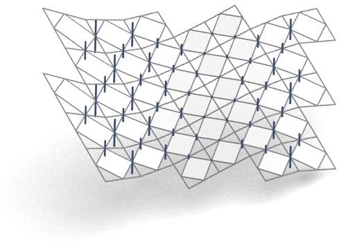
Figure 8. This developable has an inflection ruling visible as the zero level set of the length of ruling vectors. Ruling vectors are here shown without arrows.

Ruling vectors might vanish for several reasons: (i) In planar parts of a developable, rulings vectors ${\text{r}}_{\vec{e}_{i}}$ vanish and Eq. (7) is fulfilled automatically. The same is true if the developable has an inflection ruling: Fig. 8 shows that already close to the inflection ruling, vectors ${\text{r}}_{\vec{e}_{i}}$ approach zero. (ii) An individual ruling vector ${\text{r}}_{\vec{e}_{i}}$ vanishes if and only if the normal vectors ${\text{n}}_{f},{\text{n}}_{f_{i}}$ are parallel. This situation happens if faces $f,f_{i}$ are arranged along a ruling contained in the developable mesh; similar to the previous special cases, it is consistent with Eq. (7).

Remark 2.6.

In case vertex weights are equal, Eq. (7) has interesting consequences for the Gauss image. We illustrate this in the generic case (away from an inflection ruling), where a developable locally is convex. Definition 2.5 is expressed by the condition that

$${\text{n}}_{f}\times({\text{n}}_{f_{1}}-{\text{n}}_{f_{3}}),\quad{\text{n}}_{f}\times({\text{n}}_{f_{0}}-{\text{n}}_{f_{2}})\quad\text{are parallel}.$$

All vectors involved here approximately lie in a plane orthogonal to ${\text{n}}_{f}$ (namely the unit sphere’s tangent plane in ${\text{n}}_{f}$). If the quad ${\text{n}}_{f_{0}},\ldots,{\text{n}}_{f_{3}}$ were planar, then Eq. (7) would express the fact that diagonals are parallel (see the inset figure; diagonals are yellow). This characterizes quads of zero oriented area, and is nicely consistent with the fact that the Gauss image of a developable is curve-like and has zero area.

Projective Transformations

Developability is well known to be invariant under projective transformations. This property is numerically verified by Fig. 26, and is in part reflected in our approach using homogeneous coordinates (in this way projective transformations are simply expressed as linear mappings). Our constructions up to and including the computation of the ruling line fields are projectively invariant. Only the developability condition of Def. 2.5 itself, which checks equality of ruling line fields, is not. We employ such a projective transformation later — see Fig. LABEL:fig:paraboliccylinder.

Singularities of Developable Quad Meshes

Developables can exhibit geometric singularities like a cone’s vertex or the line of regression in a torsal ruled surface. The developability criterion of Def. 2.5 does not prevent singularities from emerging, and in fact, extremely singular meshes formed by the tangents of a curve may well enjoy discrete developability. We prevent such singularities by fairness imposed on the normal vector field ${\text{n}}_{f}$. Combinatorial singularities do not pose a problem, since also in this case the geometric interpretation of Eq. (7) remains valid — see Fig. 9.

Figure 9. Singularities. Left: We show a discrete-developable mesh and the good behaviour of ruling vectors ${\text{r}}_{\vec{e}}$ in the vicinity of combinatorial singularities (red). Right: This mesh exhibits a geometric singularity typical for developables, namely a sharp curve of regression. The singularity is not detectable via checking fairness of mesh polylines and is made visible by clipping by a plane. The mesh fulfills the developability condition of Def. 2.5.

2.4. Computation

All our computations are based on an optimization procedure which achieves constraints and yields low values of fairness functionals. We operate with a quad mesh $(V,E,F)$ which is thought to follow the parameter lines of a smooth surface. We have regular grid combinatorics except for isolated singularities, and we assume that we have a consistent orientation of faces. Our variables are vertices $v_{i}$, vertex weights $w_{i}$, re-weighted vertices $\widetilde{v}_{i}=w_{i}v_{i}$, a unit normal vector ${\text{n}}_{f}$ of each face $f\in F$, appropriately re-weighted edge vectors $\widetilde{\text{e}}_{02,f},\widetilde{\text{e}}_{13,f}$ per face, a ruling vector ${\text{r}}_{\vec{e}}$ for each oriented edge $\vec{e}\in E$, and re-weighted ruling vectors $\widetilde{\text{r}}_{02,f},\widetilde{\text{r}}_{13,f}$ per face.

Constraints involving vertices are

$$c_{{\text{vert}},1}(v):=\widetilde{v}_{i}-w_{i}v_{i}=0,\ \ \ c_{{\text{vert}},2}(v):=w_{i}-\omega_{i}^{2}-1.0=0.$$

We use one dummy variable $\omega_{i}$ per weight to ensure that weights remain above the threshold $1.0$. The precise value of the threshold is not relevant because all other constraints are homogeneous. Average edge vectors per face, in the notation used by Eq. (5), are defined by the constraints

$$c_{{\text{ev}},1}(f) :=\widetilde{\text{e}}_{02,f}-\big{(}(w_{0}+w_{1})(\widetilde{v}_{2}+\widetilde{v}_{3})-(w_{2}+w_{3})(\widetilde{v}_{1}+\widetilde{v}_{0})\big{)}=0,$$

$$c_{{\text{ev}},2}(f) :=\widetilde{\text{e}}_{13,f}-\big{(}(w_{1}+w_{2})(\widetilde{v}_{0}+\widetilde{v}_{3})-(w_{0}+w_{3})(\widetilde{v}_{2}+\widetilde{v}_{1})\big{)}=0$$

Vectors $\widetilde{\text{e}}_{02,f},\widetilde{\text{e}}_{13,f}$ are the previously defined average edge vectors ${\text{e}}_{02},{\text{e}}_{13}$, multiplied by a combination of weights which makes denominators vanish.

The normal vector ${\text{n}}_{f}$ is initialized according to Fig. 3, while taking the orientation into account. Our average edge vectors are precisely the diagonals in the inscribed quad depicted in Fig. 3. We therefore use the following constraints to handle normal vectors:

$$c_{{\text{norm}},1}(f) :=\langle{\text{n}}_{f},\widetilde{\text{e}}_{02,f}\rangle=0,\quad c_{{\text{norm}},2}(f):=\langle{\text{n}}_{f},\widetilde{\text{e}}_{13,f}\rangle=0,$$

$$c_{{\text{norm}},3}(f) :=\|{\text{n}}_{f}\|^{2}-1=0.$$

These normal vectors are recomputed after each round of optimization, since we cannot be sure that the implicit conditions above are sufficient to keep a consistent orientation. For every oriented half-edge $\vec{e}=v_{i}v_{j}$, we have a ruling vector ${\text{r}}_{\vec{e}}$ defined by the constraint

$$c_{\text{rul}}(\vec{e}):={\text{r}}_{\vec{e}}-{\text{n}}_{f}\times{\text{n}}_{f^{\prime}}=0,\quad\text{where}\ \vec{e}=f\cap f^{\prime},$$

with $f$ to the left and $f^{\prime}$ to the right of the half-edge $\vec{e}$. We define re-weighted ruling vectors per face by the constraints

$$c_{\text{rul},1}(f) :=\widetilde{\text{r}}_{13,f}-\big{(}(w_{1}+w_{2}){\text{r}}_{v_{1}v_{2}}+(w_{3}+w_{0})(-{\text{r}}_{v_{3}v_{0}})\big{)}=0,$$

$$c_{\text{rul},2}(f) :=\widetilde{\text{r}}_{02,f}-\big{(}(w_{0}+w_{1}){\text{r}}_{v_{0}v_{1}}+(w_{2}+w_{3})(-{\text{r}}_{v_{2}v_{3}})\big{)}=0.$$

Developability is expressed by Eq. (7):

$$c_{\text{dev}}(f):=\widetilde{\text{r}}_{13,f}\times\widetilde{\text{r}}_{02,f}=0.$$

The sums of squares of the constraints define energy functionals, $E_{{\text{vert}}}=\sum\nolimits_{v\in V,j}c_{{\text{vert}},j}(v)^{2}$, $E_{\text{norm}}=\sum\nolimits_{f\in F,j}c_{{\text{norm}},j}(f)^{2}$, and analogously for energies $E_{\text{ev}}$, $E_{\text{rul}}$, $E_{\text{dev}}$.

To ensure that the mesh polylines approximate smooth parameter lines of a surface, we employ fairness functionals: We define

$$E_{\text{fair}}^{V}=\sum\nolimits_{\text{triples}\,v_{i}v_{j}v_{k}}\|v_{i}-2v_{j}+v_{k}\|^{2},$$

where the sum is over all triples $v_{i}v_{j}v_{k}$ of successive vertices on a discrete parameter polyline. Likewise we measure the fairness of the normal field and ruling fields by energies

$$E_{\text{fair}}^{n}=\sum\limits_{\text{triples}\,f_{i}f_{j}f_{k}}\|{\text{n}}_{f_{i}}-2{\text{n}}_{f_{j}}+{\text{n}}_{f_{k}}\|^{2},E_{\text{fair}}^{r}=\sum\limits_{\text{triples}\,\vec{e}_{i},\vec{e}_{j},\vec{e}_{k}}\|{\text{r}}_{\vec{e}_{i}}-2{\text{r}}_{\vec{e}_{j}}+{\text{r}}_{\vec{e}_{k}}\|^{2}.$$

The sum in $E_{\text{fair}}^{n}$ is over all triples of successive faces arranged in a strip like shown in Fig. 5. We found that imposing fairness on the normal vector field prevents singularities like the one in Fig. 9, right. The sum in $E_{\text{fair}}^{r}$ is over triples of successive half-edges.

Summing up, in our optimization we minimize the functional

$$E=E {}_{{\text{norm}}}+\lambda_{{\text{vert}}}E_{{\text{vert}}}+\lambda_{{\text{ev}}}E_{{\text{ev}}}+\lambda_{\text{rul}}E_{\text{rul}}+\lambda_{\text{dev}}E_{\text{dev}}$$

(8) $$+\lambda_{{\text{fair}}}^{V}E_{{\text{fair}}}^{V}+\lambda_{{\text{fair}}}^{n}E_{{\text{fair}}}^{n}+\lambda_{{\text{fair}}}^{r}E_{{\text{fair}}}^{r}.$$

The weights $\lambda_{{\text{vert}}},\lambda_{\text{rul}},\ldots$ have to be chosen according to the particular application — see Table 2. In the last steps of the iteration, weights of terms used for regularization are set to $0$. This enables $E_{\text{dev}}$ to approach zero itself. Table 2 refers to the status immediately before.

Figure 11. The influence of vertex weights $w_{j}$. A coarse mesh (left) has been optimized to become developable, setting all point weights to $1$ (center) and with weights as variables (right). Gauss images show that the additional degrees of freedom provided by the weights have a beneficial influence.

Remark 2.7.

Both the definition of discrete developability and the optimization setup are much simplified if the vertex weights are equal. In such case, we can, without loss of generality, simply let $w_{i}=1$ for all $i$. Our choice of variables for optimization is guided by the empirical rule that the polynomial degree of constraints should not exceed 2. If all weights equal $1$, the number of variables is reduced not only because the weights themselves are constants now, but we also would not need edge vectors as variables — they could be replaced by a linear combination of vertices. Similarly, the average face ruling vectors could be replaced by a difference of edge ruling vectors. Figure 11 shows that the additional degrees of freedom provided by the weights have a beneficial influence, which is particularly visible for coarse meshes.

Figure 12. The influence of ruling fairness. The left- and right-hand images show results of optimization with ruling fairness disabled ($\lambda_{\text{fair}}^{r}=0$) resp., enabled. The effect is that the resulting developable does not as easily decompose into several ruled pieces.

2.5. Approximation Power of Discrete Developables

We argue that contact element nets as introduced in § 2.3 are a suitable discretization for developable surfaces, as they are capable of representing developables up to 2nd order approximations.

Locally, a surface $\Psi$ is represented as a height field $z=f(x,y)$. We approximate $f$ with a 2nd order Taylor polynomial, which yields an approximating surface $\Phi$ defined by

$$z=g(x,y)=f(0,0)+\nabla f(0,0)^{T}\binom{x}{y}+\frac{1}{2}(x\;\;y)\nabla^{2}f\binom{x}{y}.$$

If $\Psi$ is developable, then $\det\nabla^{2}f=0$ (do Carmo, 1976, p. 163). It follows that $\Phi$ is a parabolic cylinder.

Interestingly, there are many contact element nets that are developable in the sense of Def. 2.5, and whose associated B-spline surface reproduces the above-mentioned cylinder $\Phi$. The construction is the following:

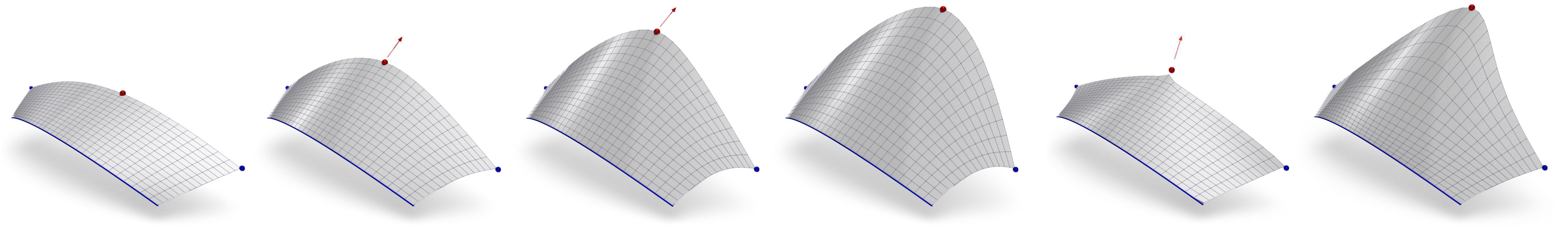
  (a)                    (b)                    (c)                     (d)                    (e)                    (f)

Figure 14. Interactive editing. The sequence of images (a)–(d) shows a developable patch being interactively modified by a user who keeps one boundary segment and two corner vertices (blue) fixed, and is dragging on another boundary vertex (red). Images (e) and (f) show the influence of the weight we give to $E_{\text{iso}}$ in our optimization. While in subfigures (a)–(d) we use isometry to the previous step for its regularizing effect, in (e) we employ isometry to the original patch. This is a constraint that is not compatible with the user’s desire to move the red vertex. Subfigure (f) is similar to (a)–(d), but with a lower weight of $E_{\text{iso}}$.

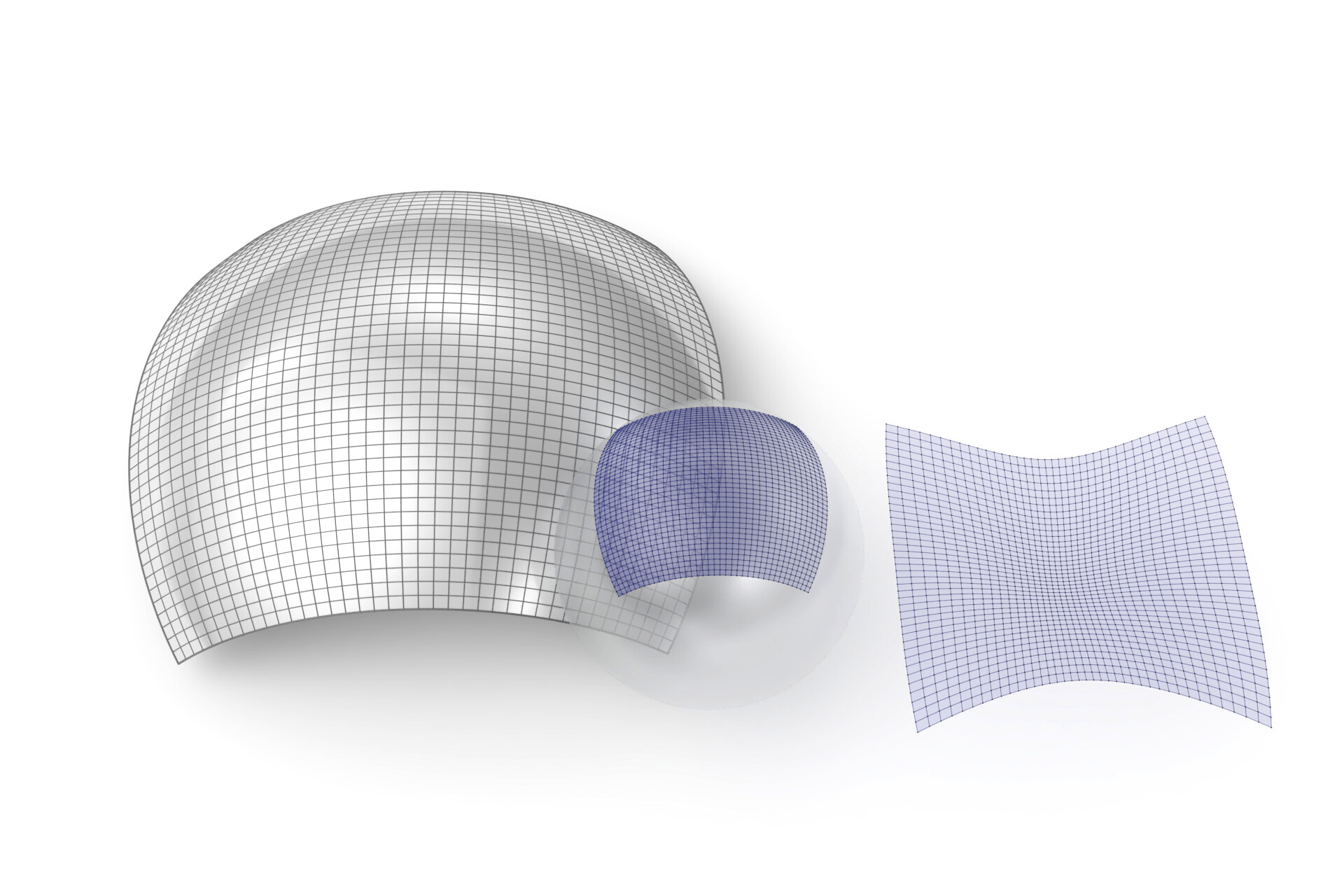
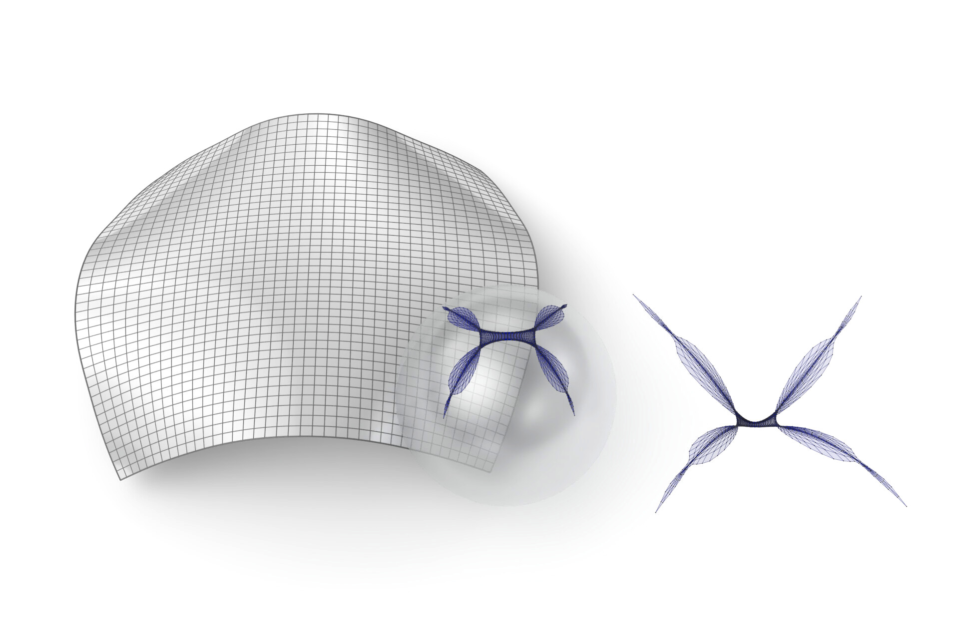
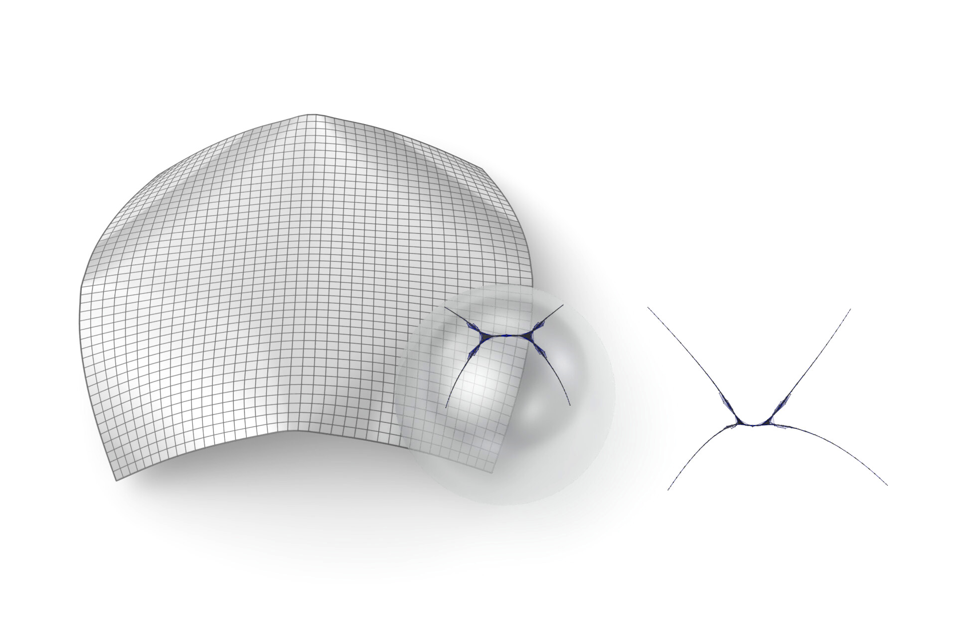
5mm 2mm 2mm 7mm4mm 2mm 1mm 7mm5mm 2mm 1mm 7mm5mm 2mm 1mm 7mm

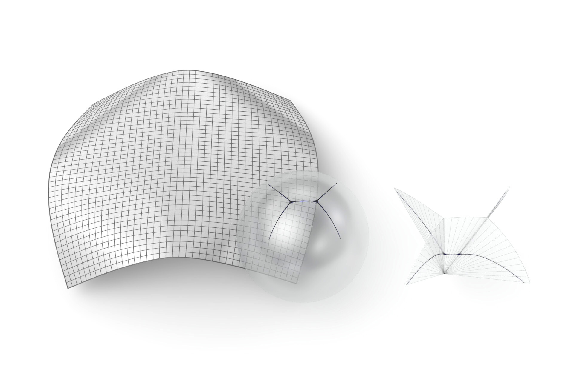
Figure 15. The action of our optimization procedure on a non-developable initial mesh. From left to right, we show the initial mesh and the result of 2, 5, and 10 rounds of optimization. After 10 rounds, both Gauss image and orthotomic surface (§ 4.2) are curve-like and no pockets of non-developability remain.

Consider the special case $g(x,y)=x^{2}$ first. Define a parametrization of the $xy$ plane and $\Phi$ by $x(u,v)=a_{1}u+b_{1}v$, $y(u,v)=a_{2}u+b_{2}v$, and $z(u,v)=x(u,v)^{2}=(a_{1}u+b_{1}v)^{2}$. Its polar form (Prautzsch et al., 2002) reads

$$G(u_{1},u_{2};\ v_{1},v_{2})=\big{(} a_{1}\frac{u_{1}+u_{2}}{2}+b_{1}\frac{v_{1}+v_{2}}{2},a_{2}\frac{u_{1}+u_{2}}{2}+b_{2}\frac{v_{1}+v_{2}}{2},$$

$$a_{1}^{2}u_{1}u_{2}+2a_{1}b_{1}\frac{u_{1}+u_{2}}{2}\frac{v_{1}+v_{2}}{2}+b_{1}^{2}v_{1}v_{2}\big{)}.$$

The function $G$ defines spline control points $v_{ij}=G(i,i+1;\ j,j+1)$, where $i,j$ run in the integers. The bi-quadratic B-spline surface with control points $v_{ij}$ exactly reproduces $\Phi$. By § 2.2.2, it is at the same time the limit surface when the net of control points undergoes Doo-Sabin subdivision.

A general parabolic cylinder $z=g(x,y)$ is either generated from the special case $z=x^{2}$ by applying an affine transformation, or directly by computing control points via the polar form of $g(x(u,v),y(u,v))$ (Prautzsch et al., 2002). Figure LABEL:fig:paraboliccylinder shows examples.

The contact element net with vertices $v_{ij}$ is exactly developable in the discrete sense. This is because discrete tangent planes $\tau_{f}$ by § 2.2.2 are tangent to $\Phi$, therefore intersect in lines parallel to the rulings of $\Phi$. It follows that all discrete rulings are parallel, implying developability.

Developables have the same tangent plane in all points of a single ruling. The parabolic cylinders mentioned above have 2nd order contact only in a single point. However, applying projective transformations yields the class of quadratic cones, which are capable of 2nd order approximation along an entire ruling (Pottmann and Wallner, 2001, § 6.1). This means that contact element nets with appropriately weighted vertices can reproduce developables up to 2nd order along an entire ruling.

Summing up, contact element nets are capable of approximating developables in the sense of a 2nd order Taylor approximation; they are even capable of exactly reproducing said Taylor approximation.

For an exact reproduction, it is not necessary that the edges of the contact net are aligned with rulings.

3. Design Tools for Developable Surfaces

We here discuss several tools for modeling developables. All are based on minimizing a target functional composed of individual energies expressing either constraints or fairness.

3.1. Interactive Editing

A basic way of design is the interactive manipulation of a surface by pulling on handles, and by requiring that certain vertices stay close to prescribed positions. Positional constraints are handled by adding an energy of the form $E_{\text{pos}}=\sum\|v_{i}-v^{*}_{i}\|^{2}$ to the total energy of Eq. (2.4). Here the sum is over all vertices $v_{i}$ for which target positions $v^{*}_{i}$ are available. Figure 14 shows how different positional constraints influence editing.

\begin{overpic}[width=303.53267pt]{figures/gliding/img_3b.jpg} \put(4.0,19.0){$\Phi$} \end{overpic}

Figure 16. Gliding Constraint. 3 positions of a developable gliding along a curve $\Phi$.

Initializing Variables For Editing

In all our examples concerning editing, vertex weights are set to $1$ and are never modified. The vertices of the mesh to be edited are assumed to be given. The remaining variables are initialized directly via their respective constraints.

The initial mesh can be arbitrary; it evolves toward developability in a way which is defined by the positional constraints imposed by the user. Figure 15 shows an example of how a non-developable initial mesh quickly becomes developable.

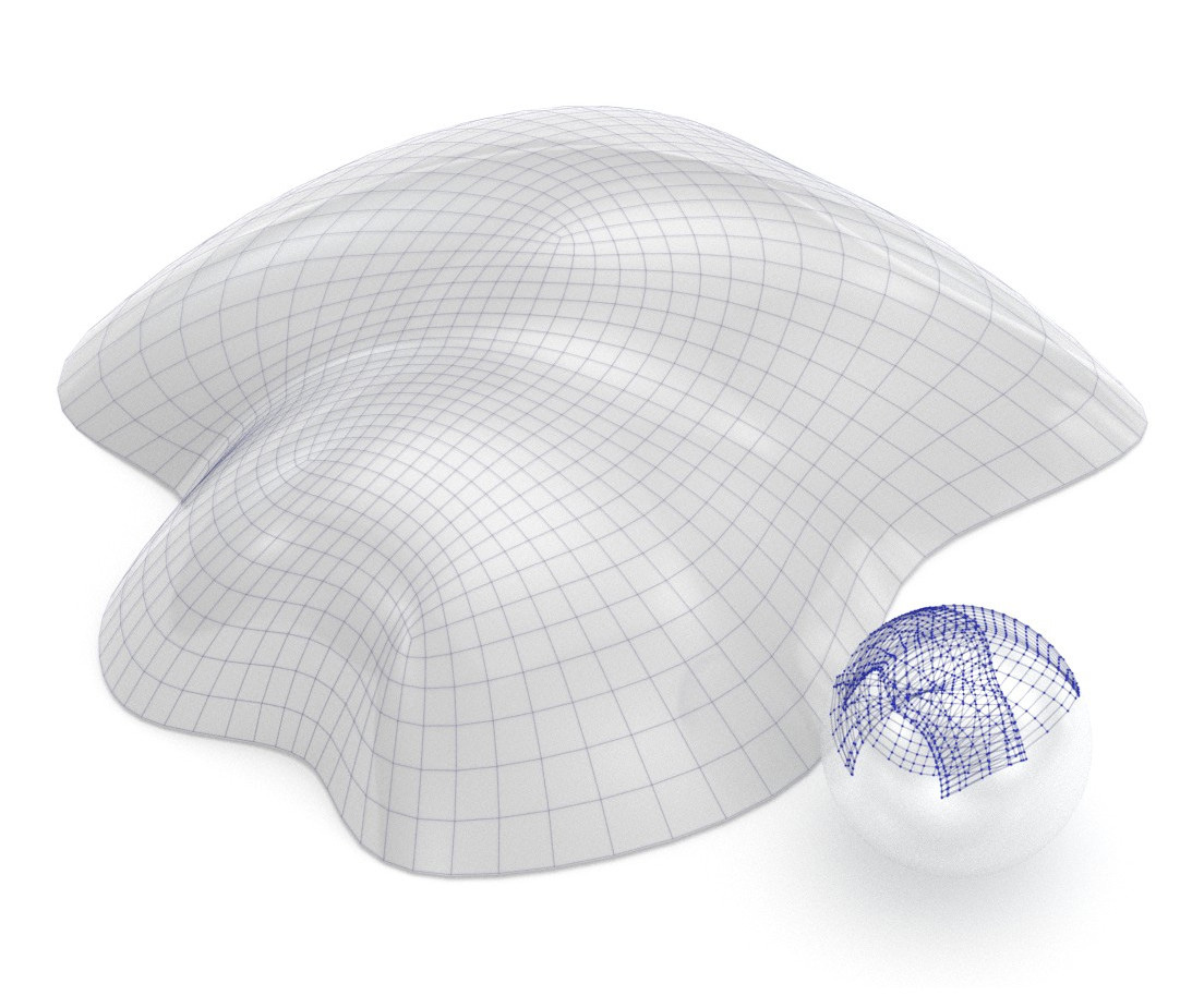
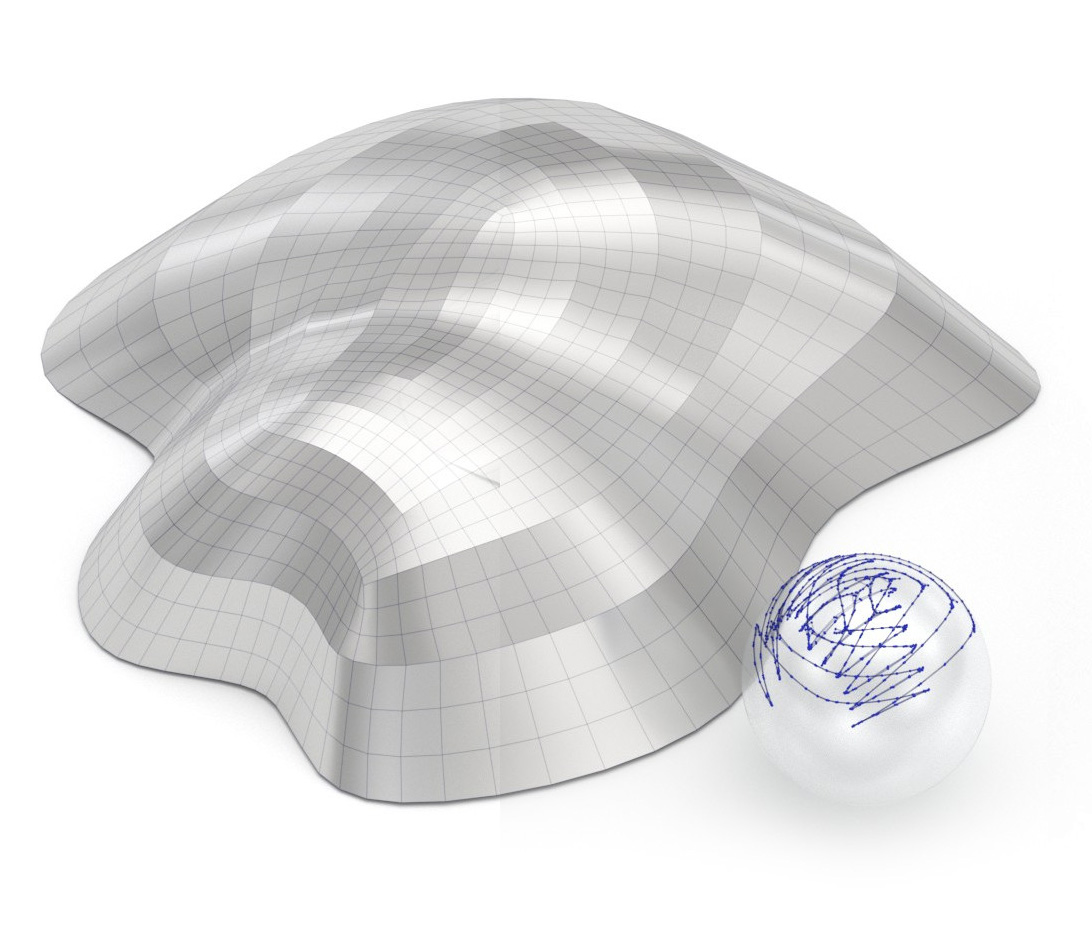
1.0cm 2mm 0.5cm 3mm

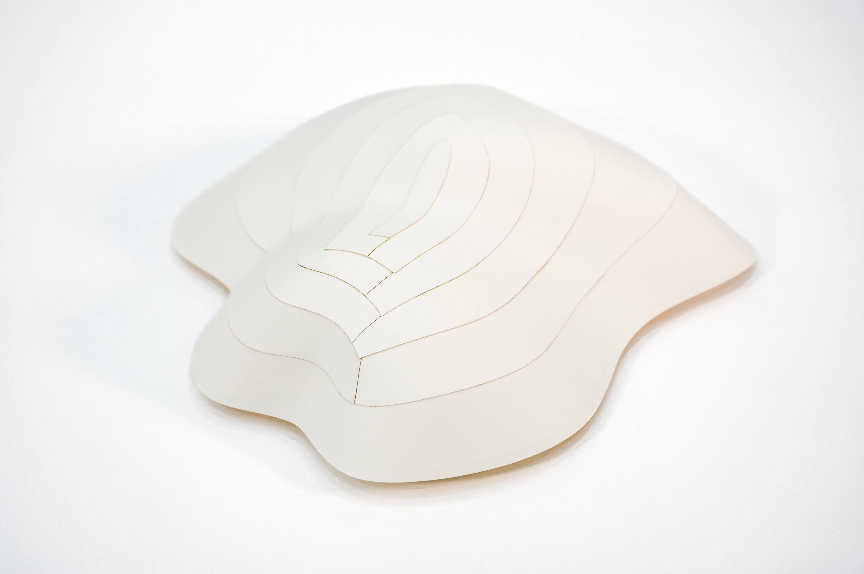
Figure 17. The surface on the left is made piecewise developable by partitioning it into strips along mesh polylines, and making those strips developable while boundaries remain fixed. We also show the Gauss image, whose curve components correspond to the developable parts of the surface. The figure on the right shows a paper model.

Gliding Constraint.

Another basic design requirement would be that our surface $M$ is to glide through a reference shape represented by a point cloud $\Phi$ (e.g. a curve). For all $p\in\Phi$ we compute the closest point projection $p^{*}\in M$ which is contained in some face $f(p)$. We now require that $p$ does not deviate from the tangent plane associated with this face, which passes through the face midpoint $b_{f(p)}$ and has normal vector ${\text{n}}_{f(p)}$. This is expressed by a low value of the energy

$$E_{\text{prox}}=\sum\nolimits_{p\ \text{active}}\langle p-b_{f(p)},\ {\text{n}}_{f(p)}\rangle^{2}$$

The sum is over all active points $p$ in the cloud $\Phi$ (which are not variables), where active means they are not too far from the variable mesh $M$. The faces $f(p)$ are recomputed in each round of the optimization. The approximation of the distance field of $M$ by distances to tangent planes is done on the basis of (Pottmann et al., 2006). It is known to be accurate to 2nd order in the case of zero distance, and it prevents unwanted effects if the pool of active points in $\Phi$ is not entirely correct. Figure 16 shows an example where a developable is gliding along a curve.

Soft Isometry Constraints as Regularizers.

In interactive modelling applications, we offer to the designer different kinds of material behaviour as illustrated by Fig. 14.

For the soft isometry constraints, we follow (Jiang et al., 2020). We express isometry between faces $f=v_{0}v_{1}v_{2}v_{3}$ and $f^{\prime}=v_{0}^{\prime}v_{1}^{\prime}v_{2}^{\prime}v_{3}^{\prime}$ by

$$c_{\text{iso},1}(f,f^{\prime}) :=\|v_{2}-v_{0}\|^{2}-\|v^{\prime}_{2}-v^{\prime}_{0}\|^{2}=0,$$

$$c_{\text{iso},2}(f,f^{\prime}) :=\|v_{3}-v_{1}\|^{2}-\|v^{\prime}_{3}-v^{\prime}_{1}\|^{2}=0,$$

$$c_{\text{iso},3}(f,f^{\prime}) :=\langle v_{2}-v_{0},v_{3}-v_{1}\rangle-\langle v^{\prime}_{2}-v^{\prime}_{0},v^{\prime}_{3}-v^{\prime}_{1}\rangle=0.$$

These constraints yield a contribution to the target functional in optimization, namely

$$E_{\text{iso}}=\sum\nolimits_{(f,f^{\prime})}\sum\nolimits_{k=1,2,3}c_{\text{iso},k}(f,f^{\prime})^{2}.$$

$\bullet$  If the design surface $M$ is to behave like an inextensible material, geometric design can be done by including the property of being isometric to the reference mesh, using the term $E_{\text{iso}}$ with a large associated weight $\lambda_{\text{iso}}$.

$\bullet$  The design surface may behave in an elastic way. In our implementation, we can choose to include the property of being isometric either to the reference mesh (with a smaller weight $\lambda_{\text{iso}}$), or to the previous state/iteration. Both provide a regularizing effect to varying extents, without pulling the surface back to its initial position. We do not claim to accurately model any exact material behavior.

3.2. Developable Lofting

A basic way how a designer may specify a developable is to prescribe two boundary curves — see Fig. 18. This procedure is referred to as lofting. Developable lofting is a problem with a long history, and early solutions for special cases. Within the framework of our optimization, we set up lofting as follows: We connect the two given curves by an arbitrary quad mesh (e.g. by a ruled surface) which we subsequently optimize.

Previous approaches to discrete developables cannot take this road easily:

$\bullet$  The semidiscrete representation of piecewise-developables by Pottmann et al. (2008) uses quad meshes with planar faces. Edges correspond either to boundary curves, or rulings. Apart from the the difficulty of having planar faces, such a mesh also cannot describe strips that are cut off in an arbitrary way, not exactly along a ruling. Since in our approach rulings are not aligned with edges, such problems do not occur.

$\bullet$  The ruling-based method of Tang et al. (2016) suffers the same deficiencies.

$\bullet$  The methods based on orthogonal geodesic nets, such as (Rabinovich et al., 2018a) and follow-up contributions, cannot describe a collection of developable strips without trimming, since the boundary curves are, in general, not geodesics.

$\bullet$  The method of Jiang et al. (2020), which is based on isometries, cannot easily solve examples like that of Fig. 18. This is because the development, which does not even exist globally, has to be initialized and then optimized simultaneously with the surface.

While some of these drawbacks might be solvable through trivial engineering solutions (such as trimming, or matching local developments), our method does not require any computational overhead, making it more efficient, and hence suitable, for interactive design.

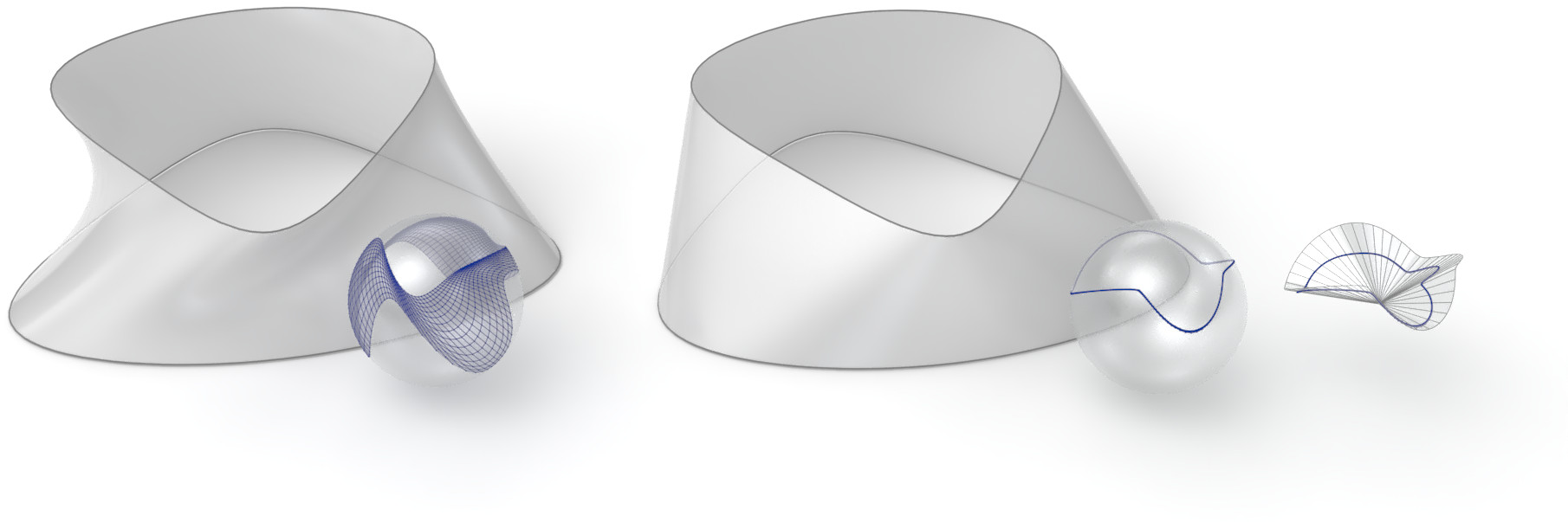
Figure 18. Developable lofting. The surface with cylinder topology on the left is optimized for developability so that the two boundary curves remain unchanged. We visualize developability not only via the Gauss image, but also with the orthotomic curve mentioned in § 4.2.

Solvability of the Lofting Problem

Lofting is actually a difficult problem, which does not need to have a smooth solution: It has many continuous solutions such as a union of cones whose vertices lie on the given boundary curves in an alternating way. Figure LABEL:fig:failwithcrease shows the behavior of our algorithm in such a failure case. A developable containing two skew lines exists and can be found (Fig. LABEL:fig:failwithcrease, bottom). However, when disabling ruling fairness, our optimization gets stuck in a local minimum and tries to find a developable whose rulings are transverse to the given boundary. In this special case, it is known that no solution exists, so we use this example to simulate a failure case. Our algorithm produces a developable with singularities at the boundary (Fig. LABEL:fig:failwithcrease, top).

Generally, developable lofting is known to be challenging. An example demonstrating the capabilities of our method is illustrated by the architectural design shown in Fig. 1.

3.3. Multiresolution Modeling

In § 2.2.2 we described the watertight spline surface associated with a quad mesh, and how it occurs as the limit of weighted Doo-Sabin subdivision. We use these tools for a multiresolution approach to modeling developables.

We start with a coarse quad mesh $M$ equipped with vertex weights. Vertices and weights are optimized such that $S^{k}M$, the result of $k$ rounds of subdivision, is a discrete developable. Here typically $k=1$ or $k=2$. The idea of this procedure is to define a near-developable spline surface $S^{\infty}M$ by a small optimized control mesh $M$. In case the result of optimization does not yield the desired quality, we subdivide, let $M:=S^{1}M$, and repeat the procedure.

The resulting spline surface consists of as many biquadratic rational Bézier patches as the mesh has faces. Our aim is to achieve a small number of patches. Figure 20 shows an example of multiresolution modeling.

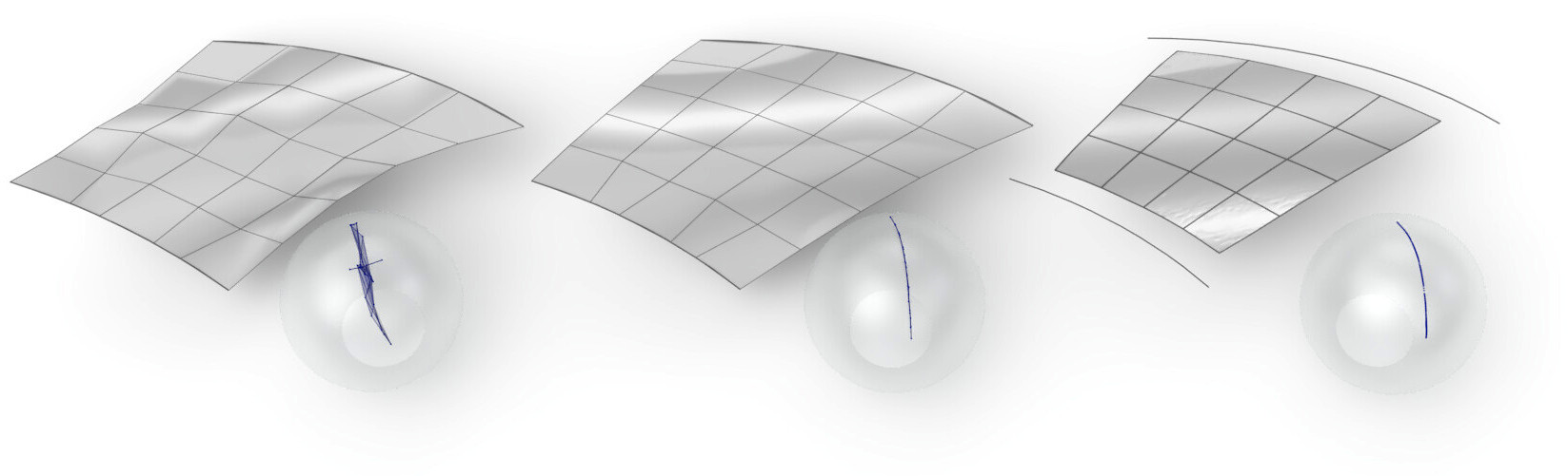
Figure 20. Combining lofting with multiresolution. Left: A coarse mesh $M$ which is optimized towards developability. The corresponding Gauss image shows that the goal has not been achieved, owing to the low resolution. Center: A coarse mesh $M^{\prime}$, constrained to the same two boundary curves as $M$, is optimized such that a subdivided mesh $S^{2}M^{\prime}$ is discrete-developable. The Gauss image of $M^{\prime}$ demonstrates a high degree of developability. Right: The biquadratic spline surface defined by $M^{\prime}$, consisting of 16 Bézier patches. It does not interpolate the boundary (for that, we would have to impose that certain face centers are constrained to the boundary, see Fig. 4, right).

4. Discussion

4.1. Implementation

All interactive design tools described in § 3 were implemented as part of Rhinoceros3D. Our plugin is a C++ dynamic-link Windows^® library that can directly interact with the Rhino application. The benefit of our implementation choice is two-fold: first, it seamlessly combines with all the existing geometry processing tools already in Rhino. This results in a powerful design environment. Secondly, Rhino is widely used within the architectural community, and thus provides a natural, broad user base for the new algorithms. Our plugin will be made available as open-source software.

The optimization of § 2.4 and § 3.1 was solved using a Levenberg-Marquardt method according to (Madsen et al., 2004, §3.2), with a damping parameter of $10^{-6}$. In the interactive application, the optimization is restarted on every user input. We terminate the optimization loop when the energy value falls below a certain threshold, or when there is no more improvement.

Our implementation uses McNeel’s openNURBS toolkit for elementary geometric manipulations, the Intel^® oneAPI Math Kernel library for efficient sparse matrix manipulations, and Intel^®’s oneMKL pardiso for solving large sparse symmetric linear systems.

\begin{overpic}[height=173.44534pt]{figures/diagrams/energies-simpledev.pdf}\color[rgb]{.7,.5,.2}\small\color[rgb]{0,0,0}\scriptsize\put(-2.0,10.0){\hbox to0.0pt{\hss{\vbox to0.0pt{\vss\hbox{$10^{-6}$}\vss}}}} \put(-2.0,32.0){\hbox to0.0pt{\hss{\vbox to0.0pt{\vss\hbox{$10^{-4}$}\vss}}}} \put(-2.0,52.0){\hbox to0.0pt{\hss{\vbox to0.0pt{\vss\hbox{$10^{-2}$}\vss}}}} \put(-2.0,72.0){\hbox to0.0pt{\hss{\vbox to0.0pt{\vss\hbox{$10^{0}$}\vss}}}} \put(22.0,0.0){\hbox to0.0pt{\hss{\vbox to0.0pt{\hbox{\scriptsize 7 iterations}\vss}}\hss}} \small\put(22.0,95.0){\hbox to0.0pt{\hss{\vbox to0.0pt{\hbox{Fig.~{}\ref{fig:simple}}\vss}}\hss}} \end{overpic}

\begin{overpic}[height=173.44534pt]{figures/diagrams/energies-hp.pdf}\small\put(35.0,95.0){\hbox to0.0pt{\hss{\vbox to0.0pt{\hbox{\contour{white}{Fig.~{}\ref{fig:failwithcrease}, top}}\vss}}\hss}} \scriptsize\put(35.0,0.0){\hbox to0.0pt{\hss{\vbox to0.0pt{\hbox{\scriptsize 400 iterations}\vss}}\hss}}\color[rgb]{0,0,0.5}\small\end{overpic}

Figure 21. Energies during optimization for Fig. LABEL:fig:simple (weights change after 4 iterations), and for the singular case of Fig. LABEL:fig:failwithcrease, top. Energy spikes correspond to buckling-like local shape changes.

The behaviour of energies during the course of optimization is exemplarily shown by Fig. 21. Table 2 provides statistics on the size of optimization problems, the choice of weights, and the time needed. Times refer to an Intel^® Xeon^® CPU E5-2695 v3 $@$ 2.30GHz x64-based processor, running 64-bit Windows^® 10. Our plugin is configured to use 64 parallel openMP threads. This was chosen to achieve interactivity for the models shown throughout the figures, but could be tuned for larger designs.

We do not give statistics for Fig. 1, Fig. 22 or Fig. 23 since these examples were interactively designed, with optimization running in the background continuously. The architectural design in Fig. 1 consists of 6 surfaces with a total of 15k faces.

Table 1. Optimization details. For selected examples, we give the number of faces, weights used in optimization, the number of individual surfaces this example consists of, the number of iterations (resp. an average number of iterations, if marked by “$\sim$”), the average time in seconds needed for a single iteration and a single surface, and the total time used for optimization.

Fig.$F_{)_{)_{)}}}$	$|F|$	$w_{\text{fair}}^{V}$	$w_{\text{fair}}^{n}$	$w_{\text{fair}}^{r}$	$w_{\text{rul}}$	$w_{\text{dev}}$​​	$w_{\text{pos}}$​​	$w_{\text{iso}}$	#surf	#it	$T_{\text{single}}^{\text{per it}}$	$T_{\text{total}}$
LABEL:fig:simple	1024	0.1	1.0		10.0	10.0		0.1	1	4	.201
		0.01	0.1		10.0	10.0		0.1		3	.207	1.4
11${}^{\text{cent}}$	99	0.1			10.0	100.0	1.0		1	162	.009	1.5
11${}^{\text{right}}$	99	0.1			10.0	100.0	1.0		1	133	.018	2.4
15	1638	0.1			10.0	100.0			1	10	.227	2.3
17	1076	0.1	0.01		1.0	10.0	100.0		6	$\sim$21	.018	2.7
18	1500	1.0	0.01		10.0	100.0	10.0		1	52	.211	11.0
LABEL:fig:failwithcrease${}^{\text{top}}$	1800	0.01	0.1		10.0	10.0	10.0	0.1	1	400	.395	158
LABEL:fig:failwithcrease${}^{\text{bot}}$	1800	0.1	0.1	2.0	10.0	100.0	10.0	0.1	1	380	.703	267
20${}^{\text{left}}$	25	0.05			10.0	100.0	1.0		1	23	.004	.092
20${}^{\text{cent}}$	25	0.05			10.0	100.0	1.0		1	106	.037	3.9

Table 2. Measuring developability. This table gives the energy $E_{\text{dev}}$ for those examples where remeshing and projective transformations take place.

Fig.	$E_{\text{dev}}^{\text{total}}$	$E_{\text{dev}}^{\text{per face}}$	$|F|$
26a	$5.5\!\cdot\!10^{-5}$	$7.4\!\cdot\!10^{-8}$	734
26b	$2.0\!\cdot\!10^{-4}$	$1.1\!\cdot\!10^{-6}$	175
26c	$1.9\!\cdot\!10^{-5}$	$2.1\!\cdot\!10^{-8}$	900
26d	$2.5\!\cdot\!10^{-5}$	$3.4\!\cdot\!10^{-8}$	734

Figure 22. Creases as a design element of piecewise developables.

4.2. Validation

Our developability condition of Def. 2.5 imposed on meshes is comparable to the requirement that the Gauss curvature of a smooth developable vanishes. The latter has a list of local and global implications, including a curve-like Gauss image and existence of rulings. These properties could be verified up to tolerances.

Visualization of Gauss Curvature

The property of the Gauss image being curve-like is a very sensitive indicator of developability. In contrast to this, visualizing the numerical values of Gauss curvature is not suitable for properly identifying developable surfaces, because the numerical errors inherent in the approximate computation of Gauss curvature are bigger than the value of Gauss curvature itself. This was confirmed in experiments on fair quad meshes sampled from mathematically correct developables, using the jet fit method of (Cazals and Pouget, 2005). For this reason, we validate developability via the Gauss image throughout this paper.

Visualization of Developability via Orthotomics

For any surface $\Phi$, reflecting a source point in all tangent planes yields the orthotomic surface $\Phi^{*}$ (Hoschek, 1985). It degenerates into a curve if and only if the original surface was developable and thus is a good visual indicator of developability — see Fig. 15 and Fig. 18.

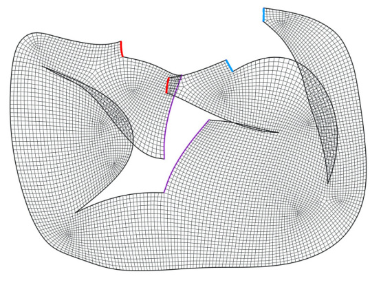
Figure 23. A developable surface made with the design tool described in § 3.1, starting from a planar mesh with 3 incisions. After cutting free every hole, a development can be computed, using the method of (Jiang et al., 2020).

4.3. Conclusion

The developability criterion for quad meshes presented in this paper has successfully been used to solve design problems with developable surfaces, which is a well-known and difficult topic with a long list of individual contributions. The fact that the edges of our developable quad meshes do not have to be aligned with special curves, represents a great practical advantage. Another advantage is the fact that we do not have to consider the actual development at the same time as the developable surface. These advantages are evident in comparison with prior work.

The method presented in this paper has a focus on the modeling of continuous deformations of discrete developable surfaces for applications in design, in line with the works of (Rabinovich et al., 2018a; Jiang et al., 2020). We observed that typically we could improve the quality of results obtained by prior work by subjecting these results to optimization by our method. Figure 24 shows an example where this has been tested on a result obtained by the method of (Rabinovich et al., 2018a). In our experience, the Gauss image test reveals that the results of (Rabinovich et al., 2018a) have the highest quality of developability among related work (Jiang et al., 2020; Sellán et al., 2020; Stein et al., 2018). Yet our method can improve the quality of developability even further.

8mm 0 8mm 0

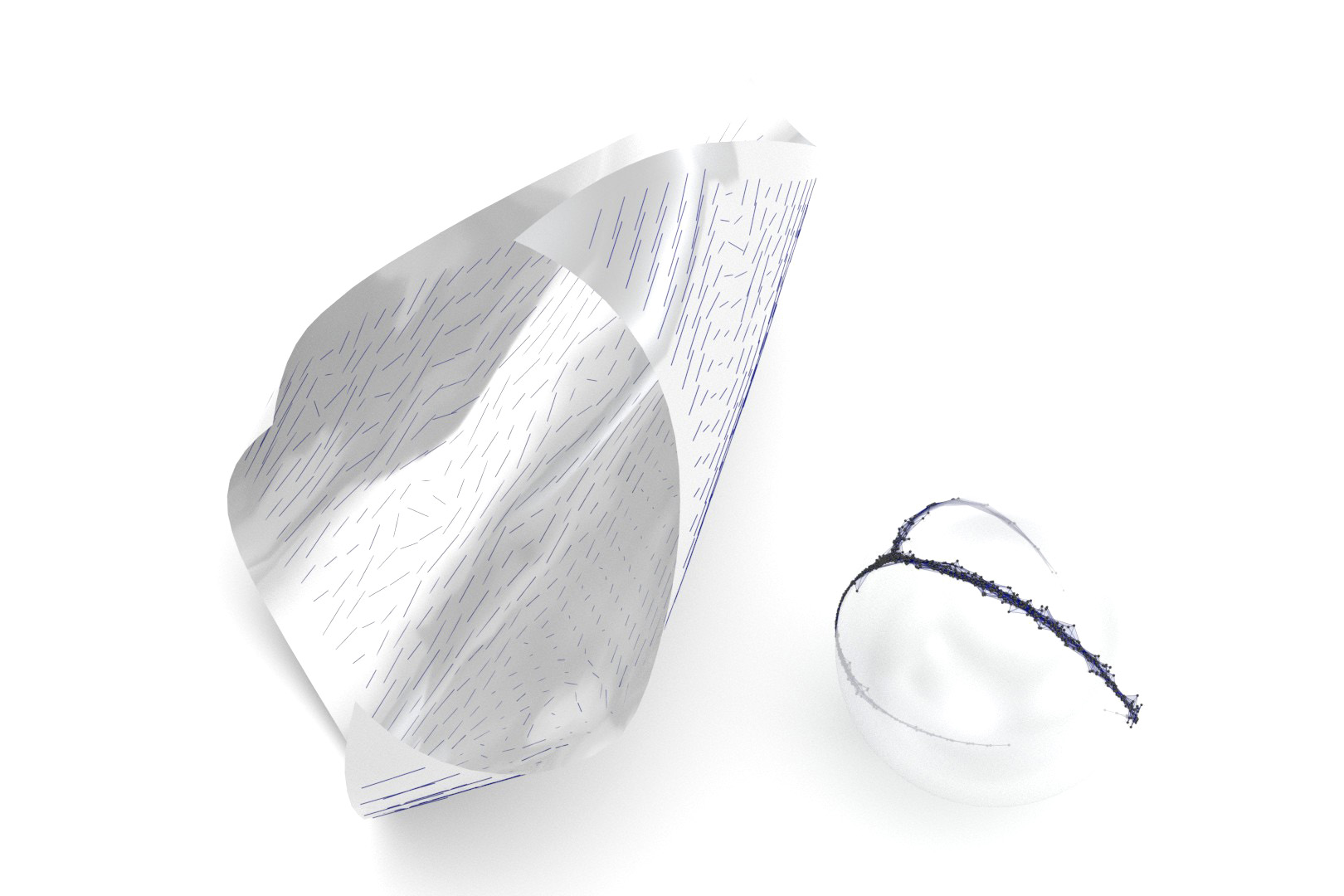
8mm 0 8mm 0

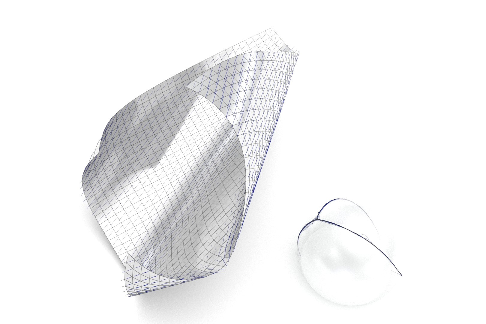
Figure 24. The mesh on the left has been created using the method of (Rabinovich et al., 2018a). We illustrate rulings and Gauss image to show that this surface is developable. Further optimization by our method improves the quality (right). The main advantage of our method compared to that of Rabinovich et al. (2018a) is that theirs works with a special parametrization, limiting its capabilities e.g. for modeling.

Our method can be used in other applications involving developables, such as guided surface approximation by piecewise developables — see Fig. 17. We do not compare approximation capabilities with previous contributions in that area (Binninger et al., 2021; Ion et al., 2020; Sellán et al., 2020; Stein et al., 2018), as currently our method would require a prior decomposition into piecewise developables. This limitation is intentional, as our focus is to incorporate design aesthetics that cannot be achieved without user-guided input.

Interactive Modeling

Our method is interactive in two ways. Firstly it can be used to interactively model developables — see Fig. 14. Secondly, we provide immediate feedback to the user: The Gauss image directly shows if developability has been achieved. The user can react and change constraints, or the weights given to constraints.

Since developables can often be defined by their boundaries, lofting is actually a very good method of design. We show several examples in previous sections; here we only point out that we can model creases as a design element, as shown in Fig. 22, as well as singularities, illustrated by Fig. 25.

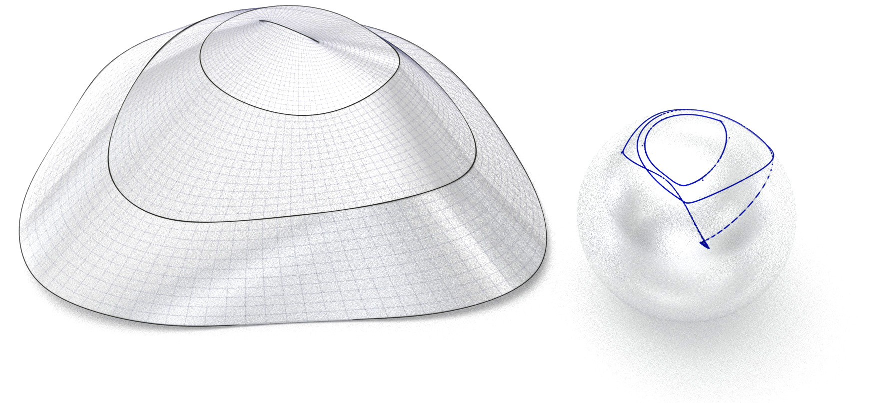
Figure 25. Lofting singularities. By choosing boundaries and optimizing the surfaces between them we achieve piecewise developability. The singularity at the top is a strip boundary that doubles back onto itself.

The developability condition proposed in this paper is almost-invariant under remeshing — see Fig. 26. This means representing a given developable mesh by another quad mesh with fair mesh polylines yields a mesh that almost fulfills our criterion of Def. 2.5 again. This is due to the underlying geometric property not being changed. This property has been used to create the examples of Fig. 23, and is extremely useful e.g. for trimming and for joining patches. We emphasize that we can work with most methods for user-guided quad remeshing, e.g. (Ebke et al., 2016).

1mm 0 0mm 0 \begin{overpic}[width=195.12767pt]{figures/evaluation/gt_20}\put(2.0,10.0){(a)}\end{overpic}     1mm 0 0mm 0 \begin{overpic}[width=195.12767pt]{figures/evaluation/gt_21}\put(2.0,10.0){(b)}\end{overpic}

1mm 0 0mm 0 \begin{overpic}[width=195.12767pt]{figures/evaluation/gt_20mesh+19edges}\put(2.0,10.0){(c)}\end{overpic}     1mm 0 0mm 0 \begin{overpic}[width=195.12767pt]{figures/evaluation/gt_23}\put(2.0,10.0){(d)}\end{overpic}

Figure 26. Invariance of developability under remeshing and projective maps. Remeshing converts mesh (a) to meshes (b), (c), and a projective transformation yields (d). $E_{\text{dev}}$ remains small — see Table 2.

Recall that in our setup we can directly leverage the projective invariance of developability, cf. § 2.3.2. Affine transformations were used in the modeling process that led to Fig. 23.

Limitations

One major limitation of our methods is geometric in nature. While an experienced user can generate developables easily, this is more difficult for a user without prior knowledge of the quirks of developable surfaces. Our implementation currently requires the user to choose weights meaningfully.

Future Research

Our aim is to publish a plugin for the software Rhino, which benefits from the possibility of conversion to NURBS format. For practical applications, material properties and tolerances need to be considered. Regarding our contribution to geometry, we are confident that it can lead to a more comprehensive theory of contact element nets.

- (1)
- Binninger et al. (2021) Alexandre Binninger, Floor Verhoeven, Philipp Herholz, and Olga Sorkine-Hornung. 2021. Developable Approximation via Gauss Image Thinning. Comput. Graph. Forum 40, 5 (2021), 289–300. Proc. SGP.
- Bobenko et al. (2010) Alexander Bobenko, Helmut Pottmann, and Johannes Wallner. 2010. A curvature theory for discrete surfaces based on mesh parallelity. Math. Annalen 348 (2010), 1–24.
- Bobenko and Suris (2007) Alexander Bobenko and Yuri Suris. 2007. On Organizing Principles of discrete differential Geometry, Geometry of spheres. Russian Math. Surveys 62, 1 (2007), 1–43.
- Bodduluri and Ravani (1993) R.M.C. Bodduluri and Bahram Ravani. 1993. Design of developable surfaces using duality between plane and point geometries. Computer-Aided Design 25 (1993), 621–632.
- Cazals and Pouget (2005) Frédéric Cazals and Marc Pouget. 2005. Estimating differential quantities using polynomial fitting of osculating jets. Computer Aided Geometric Design 22, 2 (2005), 121–146.
- Chern et al. (2018) Albert Chern, Felix Knöppel, Ulrich Pinkall, and Peter Schröder. 2018. Shape from Metric. ACM Trans. Graph. 37, 4 (2018), 63:1–17.
- do Carmo (1976) Manfredo P. do Carmo. 1976. Differential Geometry of Curves and Surfaces. Prentice-Hall, Englewood Cliffs, NJ.
- Ebke et al. (2016) Hans-Christian Ebke, Patrick Schmidt, Marcel Campen, and Leif Kobbelt. 2016. Interactively Controlled Quad Remeshing of High Resolution 3D Models. ACM Trans. Graph. 35, 6 (2016), 218:1–13.
- Guggenheimer (1963) Heinrich W Guggenheimer. 1963. Differential Geometry. McGraw-Hill, New York.
- Hoschek (1985) Josef Hoschek. 1985. Smoothing of curves and surfaces. Comput. Aided Geom. Des. 2 (1985), 97–105.
- Ion et al. (2020) Alexandra Ion, Michael Rabinovich, Philipp Herholz, and Olga Sorkine-Hornung. 2020. Shape Approximation by Developable Wrapping. ACM Trans. Graph. 39, 6 (2020), 200:1–12.
- Jiang et al. (2019) Caigui Jiang, Klara Mundilova, Florian Rist, Johannes Wallner, and Helmut Pottmann. 2019. Curve-pleated structures. ACM Trans. Graph. 38, 6 (2019), 169:1–13.
- Jiang et al. (2015) Caigui Jiang, Chengcheng Tang, Marko Tomičić, Johannes Wallner, and Helmut Pottmann. 2015. Interactive Modeling of Architectural Freeform Structures – Combining Geometry with Fabrication and Statics. In Advances in Architectural Geometry 2014. Springer, Cham, 95–108.
- Jiang et al. (2020) Caigui Jiang, Cheng Wang, Florian Rist, Johannes Wallner, and Helmut Pottmann. 2020. Quad-Mesh Based Isometric Mappings and Developable Surfaces. ACM Trans. Graph. 39, 4 (2020), 128:1–13.
- Lang and Röschel (1992) Johann Lang and Otto Röschel. 1992. Developable -Bézier Surfaces. Comput. Aided Geom. Design 9 (1992), 291–298.
- Liu et al. (2006) Yang Liu, Helmut Pottmann, Johannes Wallner, Yong-Liang Yang, and Wenping Wang. 2006. Geometric modeling with conical meshes and developable surfaces. ACM Trans. Graph. 25, 3 (2006), 681–689.
- Madsen et al. (2004) Kaj Madsen, Hans Bruun Nielsen, and Ole Tingleff. 2004. Methods for non-linear least squares problems (2nd ed.). Technical Univ. Denmark, Denmark.
- Peng et al. (2019) Chi-Han Peng, Caigui Jiang, Peter Wonka, and Helmut Pottmann. 2019. Checkerboard Patterns with Black Rectangles. ACM Trans. Graph. 38, 6 (2019), 171:1–13.
- Peters and Reif (2008) Jörg Peters and Ulrich Reif. 2008. Subdivision surfaces. Springer, Berlin Heidelberg.
- Pottmann et al. (2006) Helmut Pottmann, Qixing Huang, Yong-Liang Yang, and Shimin Hu. 2006. Geometry and convergence analysis of algorithms for registration of 3D shapes. Int. J. Computer Vision 67, 3 (2006), 277–296.
- Pottmann et al. (2008) Helmut Pottmann, Alexander Schiftner, Pengbo Bo, Heinz Schmiedhofer, Wenping Wang, Niccolo Baldassini, and Johannes Wallner. 2008. Freeform surfaces from single curved panels. ACM Trans. Graph. 27, 3 (2008), 76:1–10.
- Pottmann and Wallner (2001) Helmut Pottmann and Johannes Wallner. 2001. Computational line geometry. Springer, Berlin Heidelberg New York.
- Prautzsch et al. (2002) Hartmut Prautzsch, Wolfgang Boehm, and Marco Paluszny. 2002. Bézier and B-spline techniques. Springer, Berlin.
- Rabinovich et al. (2018a) Michael Rabinovich, Tim Hoffmann, and Olga Sorkine-Hornung. 2018a. Discrete Geodesic Nets for Modeling Developable Surfaces. ACM Trans. Graph. 37, 2 (2018), 16:1–17.
- Rabinovich et al. (2018b) Michael Rabinovich, Tim Hoffmann, and Olga Sorkine-Hornung. 2018b. The Shape Space of Discrete Orthogonal Geodesic Nets. ACM Trans. Graph. 37, 6 (2018), 228:1–17.
- Rabinovich et al. (2019) Michael Rabinovich, Tim Hoffmann, and Olga Sorkine-Hornung. 2019. Modeling Curved Folding with Freeform Deformations. ACM Trans. Graph. 38, 6 (2019), 170:1–12.
- Rörig and Szewieczek (2021) Thilo Rörig and Gudrun Szewieczek. 2021. The Ribaucour families of discrete R-congruences. Geom. Dedicata 214 (2021), 251–275.
- Sauer (1970) Robert Sauer. 1970. Differenzengeometrie. Springer, Berlin.
- Schröcker (2010) Hans-Peter Schröcker. 2010. The Bäcklund Transform of Principal Contact Element Nets. arXiv:1010.3339.
- Sellán et al. (2020) Silvia Sellán, Noam Aigerman, and Alec Jacobson. 2020. Developability of Heightfields via Rank Minimization. ACM Trans. Graph. 39, 4 (2020), 109:1–15.
- Signer et al. (2021) Madlaina Signer, Alexandra Ion, and Olga Sorkine-Hornung. 2021. Developable Metamaterials: Mass-Fabricable Metamaterials by Laser-Cutting Elastic Structures. In Proc. 2021 CHI Conf. on Human Factors in Computing Systems. ACM, 674:1–13.
- Solomon et al. (2012) Justin Solomon, Etienne Vouga, Max Wardetzky, and Eitan Grinspun. 2012. Flexible Developable Surfaces. Comput. Graph. Forum 31, 5 (2012), 1567–1576.
- Stein et al. (2018) Oded Stein, Eitan Grinspun, and Keenan Crane. 2018. Developability of Triangle Meshes. ACM Trans. Graph. 37, 4 (2018), 77:1–14.
- Tang et al. (2016) Chengcheng Tang, Pengbo Bo, Johannes Wallner, and Helmut Pottmann. 2016. Interactive design of developable surfaces. ACM Trans. Graph. 35, 2 (2016), 12:1–12.
- Verhoeven et al. (2022) Floor Verhoeven, Amir Vaxman, Tim Hoffmann, and Olga Sorkine-Hornung. 2022. Dev2PQ: Planar Quadrilateral Strip Remeshing of Developable Surfaces. ACM Trans. Graph. 41, 3 (2022), 29:1–18.
- Wolf et al. (2021) Thomas Wolf, Victor Cornillère, and Olga Sorkine-Hornung. 2021. Physically-based Book Simulation with Freeform Developable Surfaces. Comput. Graph. Forum 40, 2 (2021), 449–460.