Analysis of bistable behavior and early warning signals of extinction in a class of predator-prey models.

Abstract.

In this paper, we develop a method of detecting an early warning signal of catastrophic population collapse in a class of predator-prey models with two species of predators competing for their common prey, where the prey evolves on a faster timescale than the predators. In a parameter regime near singular Hopf bifurcation of a coexistence equilibrium point, we assume that the class of models exhibits bistability between a periodic attractor and a boundary equilibrium point, where the invariant manifolds of the coexistence equilibrium play central roles in organizing the dynamics. To determine whether a solution that starts in a vicinity of the coexistence equilibrium approaches the periodic attractor or the point attractor, we reduce the equations to a suitable normal form, which is valid near the singular Hopf bifurcation, and study its geometric structure. A key component of our study includes an analysis of the transient dynamics, characterized by their rapid oscillations with a slow variation in amplitude, by applying a moving average technique. As a result of our analysis, we could devise a method for identifying early warning signals, significantly in advance, of a future crisis that could lead to extinction of one of the predators. The analysis is applied to the predator-prey model considered in [Discrete and Continuous Dynamical Systems - B 2021, 26(10), pp. 5251-5279] and we find that our theory is in good agreement with the numerical simulations carried out for this model.

Keywords. Slow-fast systems, method of averaging, bistability, early warning signals, predator-prey models, long transients.

AMS subject classifications. 34C20, 34C29, 34D15, 37C70, 37G05, 37G35, 92D40.

1. Introduction

Identifying early warning signals for anticipating population collapses is a major focus of research in nature conservation and ecosystem management [5, 6, 8, 17, 18, 21, 29]. Often times the collapses can be catastrophic as they may not be reverted, causing huge changes in ecosystem structure and function while leading to extinction of species and substantial loss of biodiversity [2, 5]. Examples of catastrophic collapses include the dramatic extinction of passenger pigeon Estopistes migratorius in the 19th century, the collapse of the Atlantic northwest cod fishery in the early 1990s, the extinction of sea urchins Paracentrotus lividus in South Basin of Lough Hyne in Ireland in the early 2000s [2] and sharp decline of coral cover on the Great Barrier Reef [10]. Dramatic shifts in ecosystems have usually been linked to slow changes in environmental parameters that can eventually push the system over its “tipping point” [5, 8, 27, 28, 29]. However, abrupt changes in the state of an ecosystem may not be necessarily preceded by a noticeable change in the environment and the question of identifying early warning signals and the timing of a regime shift primarily remains open [5, 6, 8]. Nonetheless in many systems, regimes shift can be viewed as a property of long transient dynamics [18] and a dynamical systems modeling approach can contribute to understand such properties and study mechanisms underlying regime shifts [18, 21, 24, 26]. With this sprit, in this paper we adopt a dynamical systems approach to predict an impending transition in population dynamics of a class of three-species ecological systems exhibiting bistability between a limit cycle and a boundary equilibrium state in a parameter regime near a singular Hopf bifurcation [1, 4, 13, 15]. The goal is to predict the long-term behaviors of solutions exhibiting similar oscillatory dynamics as transients and devise a method of identifying an early warning signal significantly in advance of an abrupt transition that could lead to an extinction.

The work in this paper is inspired by the dynamics of the model studied in [25] which reads as

(4) $$\left\{\begin{array}[]{ll}\frac{dX}{dT}&=rX\left(1-\frac{X}{K}\right)-\frac{p_{1}XY}{H_{1}+X}-\frac{p_{2}XZ}{H_{2}+X}\\ \frac{dY}{dT}&=\frac{b_{1}p_{1}XY}{H_{1}+X}-d_{1}Y-a_{12}YZ\\ \frac{dZ}{dT}&=\frac{b_{2}p_{2}XZ}{H_{2}+X}-d_{2}Z-a_{21}YZ-mZ^{2},\end{array}\right.$$

where $X$ represents the population density of the prey; $Y$, $Z$ represent the densities of the two species of predators; $r>0$ and $K>0$ are the intrinsic growth rate and the carrying capacity of the prey; $p_{1}>0$ is the maximum per-capita predation rate of $Y$, $H_{1}>0$ is the semi-saturation constant which represents the prey density at which $Y$ reaches half of its maximum predation rate ($p_{1}/2$), $b_{1}>0$ is the birth-to-consumption ratio of $Y$, $d_{1}>0$ is the per-capita natural death rate of $Y$, and $a_{12}>0$ is the rate of adverse effect of $Z$ on $Y$. The other parameters $p_{2},b_{2},d_{2},H_{2},a_{21}$ are defined analogously and $m>0$ represents the intraspecific competition within $Z$.

It was observed in [25] that for suitable parameter values near a subcritical singular Hopf bifurction, system (4) exhibits bistability between a small-amplitude limit cycle and a boundary equilibrium state resulting into the extinction of one of the predators (figure 21 in [25]). It turns out that in this regime, the dynamics are organized by the invariant manifolds of a nearby saddle-focus coexistence equilibrium point, allowing a solution that starts near the coexistence equilibrium point to escape along its one-dimensional unstable manifold either towards the boundary equilibrium state or towards the nearby limit cycle. In both cases, the local dynamics near the coexistence equilibrium are characterized by rapid oscillations with a slowly varying amplitude and appear very similar, which makes any identification of an early warning signal of a population collapse extremely challenging (see figures 1 and 7).

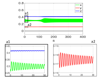
(a)

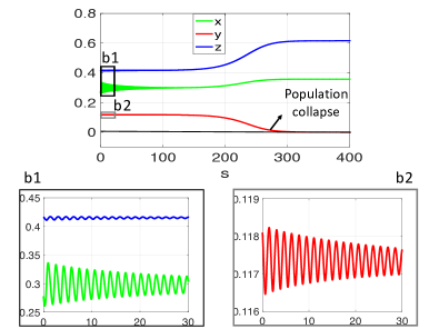
(b)

Figure 1. An illustration of bistable behavior exhibited by system (4) (or equivalently system (16) for $h=0.2649$ and other parameter values as in (17)). Both solutions exhibit similar patterns of oscillations initially as shown in the insets a1-a2 and b1-b2, but have different asymptotic behaviors. (A): Initial data chosen is $(0.2785,0.1181,0.4164)$ (B): Initial data chosen is $(0.278,0.1181,0.4165)$.

To analyze the bistable behavior, the general class of models, which includes system (4) as a special case, is reduced to a topologically equivalent class, referred to as the normal form [4], which is valid near the singular Hopf point where certain conditions on the derivatives hold. The normal form reveals the existence of a surface that separates orbits approaching the limit cycle from the point attractor as an orbit escapes along the unstable manifold of the coexistence equilibrium point, and gives insight into the geometric structures of the basins of attraction of the two attractors in the vicinity of the equilibrium point. Exploiting the separation of timescales between the rapid oscillations and a slow variation in the amplitude of oscillations near the stable manifold of the coexistence equilibrium, we partition the system into the sum of its time-averaged and fluctuating parts, and study the dynamics generated by the resultant averaged system. The averaged system encapsulates the dynamical behaviors of solutions of the original system near the coexistence equilibrium point, and yields a set of sufficient conditions for predicting their asymptotic behaviors. In addition, it aids in devising a method for finding early warning signals of the onset of a drastic change in the population of one of the species of predators. The results are in good agreement with the numerical simulations carried out for system (4).

The remainder of the paper is organized as follows. In Section 2, we present the general formulation of the class of equations and lay down the assumptions. We briefly discuss the geometric structure of system (4) and perform few numerical investigations to gain insight into the dynamics. In Section 3, we reduce the general system to a topologically equivalent form, which is valid near the singular Hopf bifurcation and analyze the equivalent system. Using the analysis, we then devise a method of detecting an early warning signal of a sudden transition in the population dynamics in Section 4. The results are supported by numerical simulations in Section 5. Finally, we summarize our conclusion in Section 6.

2. Mathematical Model

2.1. General Formulation

The class of equations under consideration is of the form

(8) $$\left\{\begin{array}[]{ll}\zeta\dot{x}&=f_{1}(x,y,z,p):=x\phi(x,y,z,p)\\ \dot{y}&=f_{2}(x,y,z,p):=y\chi(x,y,z,p)\\ \dot{z}&=f_{3}(x,y,z,p):=z\psi(x,y,z,p),\end{array}\right.$$

where $p$ is a multi-dimensional parameter in a compact subset of $\mathbb{R}^{l}$ and $\phi,\ \chi$, and $\psi$ are smooth functions having the following properties:

(H1) $\phi(0,0,0,p)>0$, $\chi(0,0,0,p)<0$, $\psi(0,0,0,p)<0$, $\phi(1,0,0,p)=0$, $\chi(1,0,0,p)>0$, $\psi(1,0,0,p)>0$ and $\phi_{x}(1,0,0,p)<0$.

(H2) $\phi(0,y,z,p)=0$ defines a smooth curve $\mathcal{T}$ in the first quadrant of the the $yz$-plane, $\Pi$, dividing $\Pi$ into two subdomains:

$$\Pi^{a}=\{(0,y,z)\in\Pi:\phi(0,y,z)<0\},\ \Pi^{r}=\{(0,y,z)\in\Pi:\phi(0,y,z)>0\}.$$

(H3) $\phi_{x}(x,y,z,p)=0$ defines a smooth curve $\mathcal{F}$ on the surface $S:=\{(x,y,z)\in\mathbb{R}^{3}:\phi(x,y,z,p)=0\}$ dividing $S$ into two smooth surfaces:

$$S^{a}=\{(x,y,z)\in S:\phi_{x}(x,y,z,p)<0\},\ S^{r}=\{(x,y,z)\in S:\phi_{x}(x,y,z,p)>0\}.$$

The overdots in (8) denote differentiation with respect to the time variable $s$, $x$ represents the population of the prey, $y$ and $z$ are the populations of the predators and $0<\zeta\ll 1$. We assume that the prey evolves on a faster timescale than the predators, a phenomenon commonly observed in many ecosystems [11, 12, 22, 23]. Condition (H1) implies that the equilibrium points $(0,0,0)$ and $(1,0,0)$ are saddles, where $(0,0,0)$ is attracting in the invariant $yz$-plane and repelling along the invariant $x$-axis while $(1,0,0)$ is attracting along the invariant $x$-axis and repelling along the $yz$ directions. Depending on $p$, (8) may admit other equilibria, some of which may lie on the $xy$-plane or the $xz$-plane. These equilibria will be referred to as the boundary equilibria and wll be denoted by $E_{xy}$ and $E_{xz}$ respectively. Rescaling $s$ by $\zeta$ and letting $t=s/\zeta$, system (8) can be reformulated as

(12) $$\left\{\begin{array}[]{ll}x^{\prime}&=f_{1}(x,y,z,p)\\ y^{\prime}&=\zeta f_{2}(x,y,z,p)\\ z^{\prime}&=\zeta f_{3}(x,y,z,p),\end{array}\right.$$

where the primes denote differentiation with respect to $t$. System (12) is referred to as the fast system, whereas (8) as the slow system. The set of equilibria of (12) in its singular limit is called the critical manifold [13], $\mathcal{M}:=\Pi\cup S$. Condition (H2) implies that $\Pi^{a}$ is normally stable while $\Pi^{r}$ is normally unstable for the limiting fast system. The normal hyperbolicity of $\Pi$ is lost along the curve of transcritical bifurcations $\mathcal{T}$. Finally, condition (H3) implies that the surface $S^{a}$ is normally attracting while $S^{r}$ is normally repelling with respect to the limiting fast system. The normal hyperbolicity of $S$ is lost via saddle-node bifurcations along the fold curve $\mathcal{F}$.

We assume that there exists a point $(\bar{x},\bar{y},\bar{z},\bar{p})$ such that the linearization of (8) at this point has a pair of eigenvalues that approach infinity as $\zeta\to 0$ and the following conditions on $f_{1}$, $f_{2}$, $f_{3}$ and their derivatives hold at $(\bar{x},\bar{y},\bar{z},\bar{p})$:

(P1) $\bar{\phi}=0,\ \bar{\chi}=0,\ \bar{\psi}=0$.

(P2) $\det J\neq 0$, where $J=\begin{pmatrix}(\bar{f}_{1})_{x}&(\bar{f}_{1})_{y}&(\bar{f}_{1})_{z}\\ (\bar{f}_{2})_{x}&(\bar{f}_{2})_{y}&(\bar{f}_{2})_{z}\\ (\bar{f}_{3})_{x}&(\bar{f}_{3})_{y}&(\bar{f}_{3})_{z}\end{pmatrix}$.

(P3) $\bar{\phi_{x}}=0$, $\bar{\phi}_{xx}\neq 0$.

(P4) $\begin{pmatrix}(\bar{f}_{1})_{y}&(\bar{f}_{1})_{z}\end{pmatrix}\begin{pmatrix}(\bar{f}_{2})_{x}\\ (\bar{f}_{3})_{x}\end{pmatrix}<0.$

(P5) $-\begin{pmatrix}(\bar{f}_{1})_{xx}&(\bar{f}_{1})_{xy}&(\bar{f}_{1})_{xz}\end{pmatrix}J^{-1}\begin{pmatrix}(\bar{f}_{1})_{p}\\ (\bar{f}_{2})_{p}\\ (\bar{f}_{3})_{p}\end{pmatrix}+(\bar{f}_{1})_{xp}\neq 0$.

Here the bars denote the values of the expressions evaluated at $(\bar{x},\bar{y},\bar{z},\bar{p})$. Note that condition (P1) indicates that $(\bar{x},\bar{y},\bar{z})$ is a coexistence equilibrium of system (8) for $p=\bar{p}$. Condition (P2) implies the existence of a smooth family of equilibria $(x_{0}(p),y_{0}(p),z_{0}(p))$ in a neighborhood of $\bar{p}$ via the implicit function theorem. Condition (P3) indicates that $(\bar{x},\bar{y},\bar{z})$ is a non-degenerate fold point. Condition (P4) implies that the linearization of system (8) at the family of equilibria $E^{*}(p)=(x_{0}(p),y_{0}(p),z_{0}(p))$ admits a pair of eigenvalues with singular imaginary parts for sufficiently small $\zeta$ (see Prop. 1 in [4]). Finally condition (P5) implies that $\frac{d\sigma}{dh}\neq 0$ at $(\bar{x},\bar{y},\bar{z},\bar{h})$, where $\sigma$ is the real part of the pair of eigenvalues with singular imaginary parts of the linearization of system (8) at the equilibrium.

The family of equilibria $(x_{0}(p),y_{0}(p),z_{0}(p))$ will be referred to as the coexistence equilibria and will be denoted by $E^{*}(p)$. The family undergoes a singular Hopf bifurcation [4, 13] at $p_{H}=\bar{p}+O(\zeta)$ for sufficiently small $\zeta>0$ (see Theorem 3.1). Finally we assume that

(Q1) there exists a family of boundary equilibria $E_{xz}(p)=(\tilde{x}(p),0,\tilde{z}(p))$ such that $\chi(\tilde{x},0,\tilde{z},p)<0$, $\phi_{x}(\tilde{x},0,\tilde{z},p)<0$, $\psi_{x}(\tilde{x},0,\tilde{z},p)>0$, $\psi_{z}(\tilde{x},0,\tilde{z},p)<0$ and $\phi_{z}(\tilde{x},0,\tilde{z},p)<0$ for all $|p-\bar{p}|=O(\zeta)$.

(Q2) The Hopf bifurcation at $p_{H}$ is subcritical, where a unique curve of saddle cycles, $\Gamma_{p}$, bifurcates and the equilibrium $E^{*}(p)=(x_{0}(p),y_{0}(p),z_{0}(p))$ switches from a saddle-focus with a two-dimensional stable and a one-dimensional unstable manifold to an unstable focus.

(Q3) If $Q_{p}:\Sigma\to\Sigma$ be a Poincaré map associated with $\Gamma_{p}$, then $Q_{p}$ undergoes a subcritical Neimark- Sacker bifurcation [20] at an $O(\zeta)$ neighborhood of $p_{H}$, resulting into the stabilization of $\Gamma_{p}$.

(Q4) The closed orbit $\Gamma_{p}$ and the boundary equilibrium $E_{xz}$ lie on opposite sides of $\Sigma$, where $\Sigma$ is the tangent plane to the local stable manifold of $E^{*}(p)$. Furthermore, ${\bf{F}}\cdot{\bf{n}}>0$, where ${\bf{F}}$ is the vector field corresponding to system (8) and ${\bf{n}}$ is the normal vector to $\Sigma$ pointing towards the lower-half space, $\Sigma^{-}$, containing $E_{xz}(p)$.

(Q5) The unstable manifold of the saddle-focus equilibrium $E^{*}(p)$ spirals onto the stable manifold of $\Gamma_{p}$ in the upper-half space $\Sigma^{+}$, whereas it tends to the stable manifold of $E_{xz}(p)$ in the lower-half space $\Sigma^{-}$ for all $|p-p_{H}|=O(\zeta)$.

Condition (Q1) implies that the family of fixed points $E_{xz}(p)$ is locally asymptotically stable for all $p$ in an $O(\zeta)$ neighborhood of $\bar{p}$. (Q4) indicates that the lower half-space $\Sigma^{-}$ is positively invariant with respect to the flow generated by the vector field in (8). (Q5) indicates that there exists a maximal open set $\mathcal{U}\subset\Sigma^{+}$ around $E^{*}$ such that the flow from $U$ asymptotically approaches $\Gamma_{p}$ in the parameter regime in which it is asymptotically stable. Conditions (Q1), (Q3) and (Q5) indicate that system (8) has a point attractor $E_{xz}$ coexisting with $\Gamma_{p}$ in an $O(\zeta)$ neighborhood of ${p_{H}}$.

2.2. A predator-prey model

An example of the class (8) that satisfies conditions (H1)-(H3) along with (P1)-(P5) and (Q1)-(Q5) is system (4) which in its non-dimensional form (see [25] for the details) reads as

(16) $$\left\{\begin{array}[]{ll}\zeta\dot{x}&=x\left(1-x-\frac{y}{\beta_{1}+x}-\frac{z}{\beta_{2}+x}\right):=x\phi(x,y,z)\\ \dot{y}&=y\left(\frac{x}{\beta_{1}+x}-c-\alpha_{12}z\right):=y\chi(x,y,z)\\ \dot{z}&=z\left(\frac{x}{\beta_{2}+x}-d-\alpha_{21}y-hz\right):=z\psi(x,y,z).\end{array}\right.$$

In (16), the overdots denote differentiation with respect to the slow time $s$ and $\phi=0$, $\chi=0$, and $\psi=0$ are the nontrivial $x$, $y$, and $z$-nullclines respectively. The parameter $\zeta$ measures the ratio of the growth rates of the predators to the prey and satisfies $0<\zeta\ll 1$. The dimensionless parameters $\beta_{1}$, $c$ and $\alpha_{12}$ respectively represent the predation efficiency [11], rescaled mortality rate and rescaled interspecific competition coefficient of $y$. The parameters $\beta_{2}$, $d$ and $\alpha_{21}$ are analogously defined. The parameter $h$ represents the rescaled intraspecific competition coefficient within $z$. As in [25], we will assume that $0<c,\ d,\ \beta_{1},\ \beta_{2}\ \alpha_{12},\ \alpha_{21}<1$. It is easy to verify that system (16) satisfies the assumptions stated in (H1)-(H3).

In the singular limit, the reduced flow corresponding to (16), restricted to the surface $S$, has singularities along the fold curve $\mathcal{F}$, referred to as the folded singularities or canard points [13]. These singularities are analyzed by desingularizing the reduced flow (see [25]). If an equilibrium of (16) and a folded singularity merge together and split again, interchanging their type and stability, then a folded saddle-node bifurcation of type II (FSN II) occurs [13], followed by a singular Hopf bifurcation in an $O(\zeta)$ neighborhood of the FSN II bifurcation.

2.3. Numerical investigations of system (16)

Treating the intraspecific competition $h$ as the primary bifurcation parameter and the predation efficiency $\beta_{1}$ as the secondary parameter, system (16) was analyzed in [25]. In this paper, we will also treat $h$ as the input parameter and fix the other parameter values to

(17) $$\beta_{1}=0.1923,\ \beta_{2}=0.6,\ c=0.4,\ d=0.21,\ \alpha_{12}=0.5,\ \alpha_{21}=0.1,\ \zeta=0.01.$$

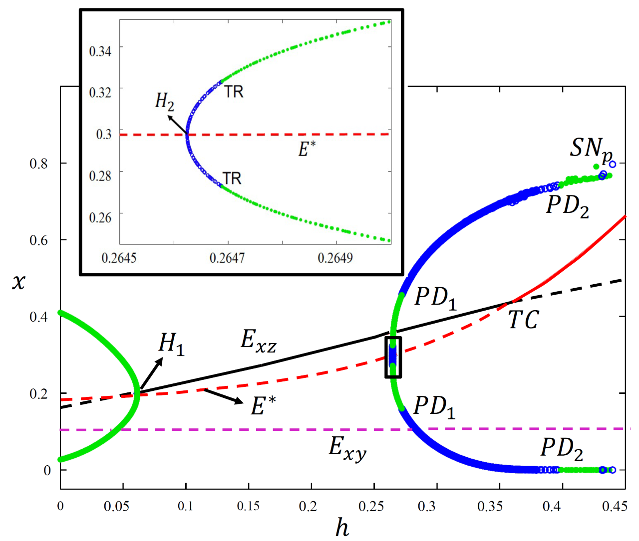
Figure 2. One-parameter bifurcation diagram of system (16) as $h$ is varied. Stable branches of equilibria are represented in solid and unstable branches by dotted curves. Stable limit cycles are in green and unstable cycles are in blue. $H_{1}$, $H_{2}$: Hopf bifurcation, $PD_{1},PD_{2}$: period-doubling bifurcation, $TR$: torus bifrucation, $SN_{p}$: saddle-node of periodics, $TC$: transcritical bifurcation.

Using XPPAUT [14], we compute a one-parameter bifurcation diagram as shown in figure 2, where the maximum norm is considered along the vertical axis. We note from figure 2 that the boundary equilibrium state $E_{xy}$ is always unstable (exists as a saddle in this parameter range), whereas the stabilities of the boundary equilibrium $E_{xz}$ and the coexistence equilibrium state $E^{*}$ change with $h$. For larger values of $h$, $E_{xz}$ exists as an unstable focus/node and $E^{*}$ as a stable node until the two equilibria branches undergo a transcritical bifurcation $TC\approx 0.3577$. The coexistence equilibrium $E^{*}$ persists as a saddle or a sadle-focus with one positive and two complex (with negative real parts) eigenvalues for $h<0.3577$ until it undergoes a subcritical Hopf bifurcation $H_{2}\approx 0.2646$ and switches to an unstable focus, whereas $E_{xz}$ persists as a locally asymptotically stable node/focus until it undergoes a supercritical Hopf bifurcation at $H_{1}\approx 0.0613$, giving birth to a family of stable periodic orbits that lie in the invariant $xz$-plane. Nearby $H_{2}$, a subcritical torus bifurcation occurs at $TR\approx 0.2647$, resulting into the stabilization of the saddle cycles $\Gamma_{h}$ born at $H_{2}$. On further increasing $h$, the family of periodic attractors $\Gamma_{h}$ loses stability at a period-doubling bifurcation $PD_{1}\approx 0.272$ and re-gains stability at a second period-doubling bifurcation $PD_{2}\approx 0.3986$. Mixed-mode oscillations [7, 13] are observed in this regime. Soon after, the family experiences a saddle-node bifurcation $SN_{p}\approx 0.43143$, after which relaxation oscillations are observed. Further details of the bifurcation diagram are beyond the scope of this paper.

An FSN II bifurcation occurs at $\bar{h}\approx 0.2656$ where the coordinates of the equilibrium $E^{*}$ are $(\bar{x},\bar{y},\bar{z})\approx(0.2987,0.1167,0.4167)$. It is easy to check that system (16) satisfies (P1)-(P5) at $(\bar{x},\bar{y},\bar{z},\bar{h})$. Note that $H_{2}$ and $TR$ lie in an $O(\zeta)$ neighborhood of $\bar{h}$. In a small parameter regime past $TR$, where $E^{*}$ is a saddle-focus and $E_{xz}$ is locally asymptotically stable, the system exhibits bistability between $E_{xz}$ and $\Gamma$ as shown in figure 1 (also see figure 7), and thus system (16) satisfies conditions (Q1)-(Q5). We note that in the bistable regime, the local dynamics of the solutions near $E^{*}$ are very similar, and thus the invariant manifolds of the equilibrium $E^{*}$ play central roles in organizing the dynamics.

One way of analyzing the bistable behavior is by numerical computation of the invariant manifolds of the equilibria and the limit cycle and studying the dynamics generated by their interaction. Computations of such manifolds are numerically challenging as they involve stiffness related issues. Another approach is to reduce the system to a topologically equivalent form near the FSN II point on which a simpler geometric treatment can be applied. In this paper, we will take the latter approach. To characterize the local dynamics near $E^{*}$, we will reduce system (8) to its normal form, which will be valid in a small neighborhood of $E^{*}$, and analyze it. The analysis will be then used to find an early warning sign of an impending population shift.

3. Normal form near the singular Hopf bifurcation

A normal form for singular Hopf bifurcation in one-fast and two-slow variables has been explicitly derived by Braaksma [4]. We will follow [4] to reduce system (8) to its normal form (also see [26]). The reduction allows us to explicitly calculate Hopf bifurcation analytically as stated in the next theorem.

Theorem 3.1.

Under conditions (P1)-(P5), system (8) can be written in the normal form:

(21) $$\left\{\begin{array}[]{ll}\frac{du}{d\tau}&=v+\frac{u^{2}}{2}+\delta(\alpha(p)u+F_{13}uw+\frac{1}{6}F_{111}u^{3})+O(\delta^{2})\\ \frac{dv}{d\tau}&=-u+O(\delta^{2})\\ \frac{dw}{d\tau}&=\delta(H_{3}w+\frac{1}{2}H_{11}u^{2})+O(\delta^{2}),\end{array}\right.$$

where $\tau=\frac{s}{\delta}$ with $\delta=\frac{\sqrt{\zeta}}{{\omega}}$ and

$$\left\{\begin{array}[]{ll}\omega&=\sqrt{-\bar{x}(\bar{y}\bar{\phi_{y}}\bar{\chi_{x}}+\bar{z}\bar{\phi_{z}}\bar{\psi_{x}})},\\[5.0pt] F_{13}&=\bar{x}\bar{\phi_{z}}(\bar{z}\bar{\psi_{z}}-\bar{y}\bar{\chi_{y}})+\frac{\bar{x}}{\bar{\phi_{y}}}(\bar{y}\bar{\phi^{2}_{y}}\bar{\chi_{z}}-\bar{z}\bar{\phi^{2}_{z}}\bar{\psi_{y}})+\frac{\omega^{2}}{\bar{\phi_{xx}}\bar{\phi_{y}}}(\bar{\phi_{xz}}\bar{\phi_{y}}-\bar{\phi_{xy}}\bar{\phi_{z}}),\\[5.0pt] F_{111}&=\frac{\omega^{2}}{\bar{x}^{2}\bar{\phi^{2}_{xx}}}(3\bar{\phi}_{xx}+\bar{x}\bar{\phi}_{xxx})+\frac{\bar{x}}{\omega^{2}}[\bar{y}\bar{\chi_{x}}(\bar{y}\bar{\phi_{y}}\bar{\chi_{y}}+\bar{z}\bar{\phi_{z}}\bar{\psi_{y}})+\bar{z}\bar{\psi_{x}}(\bar{y}\bar{\phi_{y}}\bar{\chi_{z}}+\bar{z}\bar{\phi_{z}}\bar{\psi_{z}})]\\ &+\frac{1}{\bar{x}\bar{\phi}_{xx}}[\bar{y}\bar{\chi_{x}}(\bar{\phi_{y}}+\bar{x}\bar{\phi}_{xy})+\bar{z}\bar{\psi_{x}}(\bar{\phi_{z}}+\bar{x}\bar{\phi}_{xz})+\bar{x}(\bar{y}\bar{\phi_{y}}\bar{\chi}_{xx}+\bar{z}\bar{\phi_{z}}\bar{\psi}_{xx})],\\[7.0pt] H_{3}&=\frac{\bar{x}\bar{y}\bar{z}}{\omega^{2}}[\bar{\psi_{x}}(\bar{\phi_{y}}\bar{\chi_{z}}-\bar{\phi_{z}}\bar{\chi_{y}})-\bar{\chi_{x}}(\bar{\phi_{y}}\bar{\psi_{z}}-\bar{\phi_{z}}\bar{\psi_{y}})],\\[5.0pt] H_{11}&=\frac{\bar{x}\bar{y}\bar{z}}{\omega^{4}}\bar{\phi_{y}}(\bar{\psi_{x}}-\bar{\chi_{x}})\left(\bar{y}\bar{\chi_{x}}\bar{\chi_{y}}+\bar{z}\bar{\psi_{x}}\bar{\psi_{z}}\right)+\frac{\bar{y}\bar{z}}{\omega^{2}\bar{x}\bar{\phi}_{xx}}\bar{\phi_{y}}\left(\bar{z}\bar{\psi_{x}}\bar{\chi}_{xx}-\bar{x}\bar{\chi_{x}}\bar{\psi}_{xx}\right),\\[5.0pt] \alpha(p)&=\left\{-\begin{pmatrix}(\bar{f}_{1})_{xx}&(\bar{f}_{1})_{xy}&(\bar{f}_{1})_{xz}\end{pmatrix}J^{-1}\begin{pmatrix}(\bar{f}_{1})_{p}\\ (\bar{f}_{2})_{p}\\ (\bar{f}_{3})_{p}\end{pmatrix}+(\bar{f}_{1})_{xp}\right\}\Big{(}\frac{p-\bar{p}}{\zeta}\Big{)}\\ &-\frac{1}{\omega^{2}}\{(\bar{f}_{1})_{y}[(\bar{f}_{2})_{y}(\bar{f}_{2})_{x}+(\bar{f}_{2})_{z}(\bar{f}_{3})_{x}]+(\bar{f}_{1})_{z}[(\bar{f}_{3})_{y}(\bar{f}_{2})_{x}+(\bar{f}_{3})_{z}(\bar{f}_{3})_{x})]\}.\end{array}\right.$$

The normal form is valid for $(x,y,z,p)=(\bar{x}+O(\sqrt{\zeta}),\bar{y}+O(\zeta),\bar{z}+O(\zeta),\bar{p}+O(\zeta))$. Furthermore, system (8) undergoes a Hopf bifurcation at $p=\bar{p}+\zeta A+O(\zeta^{3/2})$ for sufficiently small $\zeta>0$, where $A$ is the solution of the equation

$$\left\{-\begin{pmatrix}(\bar{f}_{1})_{xx}&(\bar{f}_{1})_{xy}&(\bar{f}_{1})_{xz}\end{pmatrix}J^{-1}\begin{pmatrix}(\bar{f}_{1})_{p}\\ (\bar{f}_{2})_{p}\\ (\bar{f}_{3})_{p}\end{pmatrix}+(\bar{f}_{1})_{xp}\right\}A = \frac{1}{\omega^{2}}\{(\bar{f}_{1})_{y}[(\bar{f}_{2})_{y}(\bar{f}_{2})_{x}+(\bar{f}_{2})_{z}(\bar{f}_{3})_{x}]$$

$$+ (\bar{f}_{1})_{z}[(\bar{f}_{3})_{y}(\bar{f}_{2})_{x}+(\bar{f}_{3})_{z}(\bar{f}_{3})_{x})]\}.$$

The Hopf bifurcation is super(sub)critical if the first Lyapunov coefficient

(23) $$l_{1}(0)=\frac{\delta}{4}\Big{(}\frac{1}{2}F_{111}-\frac{F_{13}H_{11}}{H_{3}}\Big{)}<(>)0.$$

We refer to the work of Braaksma (Theorems 1 and 2 in [4]) for the detailed proof. With extensive algebraic calculations, we can write $(u,v,w)$ in terms of the original coordinates $(x,y,z)$. The transformations are given in the Appendix.

3.1. Analysis of the normal form

We will employ system (21) to study the dynamics of system (8) near the equilibrium $E^{*}=(x_{0}(p),y_{0}(p),z_{0}(p))$ for $p$ in an $O(\zeta)$ neighborhood of $\bar{p}$. In the normal form variables, $E^{*}$ is mapped to the origin and will be denoted by $q_{e}$. We note that the eigenvalues of the variational matrix of (21) at the equilibrium $q_{e}$ up to higher order terms are

(24) $$\rho_{1}=\delta H_{3},\ \rho_{2,3}=\frac{1}{2}\Big{[}\alpha\delta\pm\sqrt{\alpha^{2}\delta^{2}-4}\Big{]}.$$

If $H_{3}<0$, then $q_{e}$ is a stable node or a stable spiral for $\alpha<0$, while it is a saddle-focus with two-dimensional unstable and one-dimensional stable manifold for $0<\alpha<2/\delta$. On the other hand, if $H_{3}>0$, then $q_{e}$ is an unstable node/spiral for $0<\alpha<2/\delta$, while it is a saddle-focus with two-dimensional stable and one-dimensional unstable manifold for $\alpha<0$.

Recalling that (8) satisfies (Q2)-(Q5) near $\bar{p}$, it follows that system (21) also satisfies those conditions near $q_{e}$. By (Q2), $q_{e}$ switches from an unstable focus to a saddle-focus at $\alpha=0$, hence we must have that $H_{3}>0$. Condition (Q3) implies that there exists a family of attracting limit cycles, $\Gamma_{\alpha}$, in system (21) for $\alpha\in(\alpha_{s},\alpha_{e})$, where $O(\delta^{2})=\alpha_{s},\alpha_{e}<0$. Assuming that $\Gamma_{\alpha}$ lies on the upper-half space $\{w>0\}$ and the equilibrium $E_{xz}$ of system (8) lies on the lower half-space $\{w<0\}$, it then follows from (Q4) that the flow generated by (21) on the tangent plane of the stable manifold of $q_{e}$ points towards the lower-half space. Hence we must have $H_{11}<0$. Condition (Q5) implies that for all $\alpha\in(\alpha_{e},0)$, the unstable manifold of $q_{e}$ tends to the stable manifold of $\Gamma_{\alpha}$ in the upper-half space $\{w>0\}$. Finally, by (Q2), the Hopf bifurcation is subcritical, hence $l_{1}(0)>0$ in (23).

3.1.1. Linear Analysis near $q_{e}$

For $\alpha<0$ and $H_{3}>0$, the flow generated by (21) up to the first order is given by

(29) $$\left\{\begin{array}[]{ll}u(\tau)&=Ae^{\frac{\alpha\delta\tau}{2}}\sin(\vartheta\tau+\phi_{1}),\\ v(\tau)&=Ae^{\frac{\alpha\delta\tau}{2}}\sin(\vartheta\tau+\phi_{2}),\\ w(\tau)&=e^{\delta H_{3}\tau}\Big{(}w_{0}+\frac{\delta H_{11}}{2}\Big{(}C+\frac{4\vartheta^{2}u_{0}^{2}+(2v_{0}+\alpha\delta u_{0})^{2}}{8\vartheta^{2}\delta(\alpha-H_{3})}\Big{)}\Big{)}\\ &+\frac{\delta}{2}H_{11}e^{\alpha\delta\tau}\Big{[}C\cos(2\vartheta\tau)+D\sin(2\vartheta\tau)+\frac{4\vartheta^{2}u_{0}^{2}+(2v_{0}+\alpha\delta u_{0})^{2}}{8\vartheta^{2}\delta(\alpha-H_{3})}\Big{]},\end{array}\right.$$

where $(u(0),v(0),w(0))=(u_{0},v_{0},w_{0})$ and

$$\vartheta = \sqrt{1-\frac{\alpha^{2}\delta^{2}}{4}},\ A=\frac{1}{\vartheta}\sqrt{u_{0}^{2}+\alpha\delta u_{0}v_{0}+v_{0}^{2}},\ \phi_{1}=\tan^{-1}\Big{(}\frac{2\vartheta u_{0}}{2v_{0}+\alpha\delta u_{0}}\Big{)},$$

$$\phi_{2} = \tan^{-1}\Big{(}-\frac{2\vartheta v_{0}}{2u_{0}+\alpha\delta v_{0}}\Big{)},$$

$$C = \frac{\delta(\alpha-H_{3})(4\vartheta^{2}u_{0}^{2}-(2v_{0}+\alpha\delta u_{0})^{2})-8\vartheta^{3}u_{0}(2v_{0}+\alpha\delta u_{0})}{8\vartheta^{2}(4\vartheta^{2}+\delta^{2}(\alpha-H_{3})^{2})},$$

$$D = \frac{4\vartheta^{2}u_{0}^{2}-(2v_{0}+\alpha\delta u_{0})^{2}+2\delta(\alpha-H_{3})u_{0}(2v_{0}+\alpha\delta u_{0})}{4\vartheta(4\vartheta^{2}+\delta^{2}(\alpha-H_{3})^{2})}.$$

In this case, the two-dimensional local stable manifold $W_{\mathrm{loc}}^{s}(q_{e})$ can be expressed as a graph [15, 20]

$$w=\Theta(u,v,\delta) = \frac{1}{2}\Theta_{uu}^{0}u^{2}+\Theta_{uv}^{0}uv+\frac{1}{2}\Theta_{vv}^{0}v^{2}+O(3)+\delta\Big{(}\frac{1}{2}\Theta_{uu}^{1}u^{2}+\Theta_{uv}^{1}uv+\frac{1}{2}\Theta_{vv}^{1}v^{2}$$

$$+ O(3)\Big{)}+O(\delta^{2}),$$

where $O(3)$ represents cubic and higher-order terms in $u$ and $v$. The function $\Theta$ can be determined by solving the equation $\frac{d\Theta}{d\tau}=\delta(H_{3}\Theta+\frac{1}{2}H_{11}u^{2})+O(\delta^{2})$. Inserting the expression for $w$ in the above equation yields that

$$\Big{[}(\Theta_{uu}^{0}-\Theta_{vv}^{0})uv+\Theta_{uv}^{0}v^{2}-\Theta_{uv}^{0}u^{2}\Big{]}+\delta\Big{[}(\Theta_{uu}^{1}-\Theta_{vv}^{1}+\alpha\Theta_{uv}^{0})uv+\Theta_{uv}^{1}v^{2}+(\alpha\Theta_{uu}^{0}-\Theta_{uv}^{1})u^{2}\Big{]}$$

$$=\delta\Big{[}\Big{(}\frac{H_{11}}{2}+\frac{H_{3}}{2}\Theta_{uu}^{0}\Big{)}u^{2}+H_{3}\Theta_{uv}^{0}uv+\frac{H_{3}}{2}\Theta_{vv}^{0}v^{2}\Big{]}+O(\delta^{2})+O(3).$$

Equating the coefficients of like terms we obtain an approximation for $W_{\mathrm{loc}}^{s}(q_{e})$:

(30) $$w=\Theta(u,v,\delta)=\frac{H_{11}}{4(\alpha-H_{3})}(u^{2}+v^{2})+\frac{\delta H_{3}H_{11}}{4(\alpha-H_{3})}uv+O(3)+O(\delta).$$

3.1.2. Parametrization of the slow variable in system (21)

For a fixed $O(\delta^{2})=\alpha<0$, one may replace the slow variable $w$ in system (21) by a parameter $\lambda$ to obtain insight into the dynamics of the fast variables. The fast variables $(u,v)$ are then governed by the parametrized system

(33) $$\left\{\begin{array}[]{ll}\frac{du}{d\tau}&=\delta(\alpha+F_{13}\lambda)u+v+\frac{u^{2}}{2}+\frac{\delta}{6}F_{111}u^{3}\\ \frac{dv}{d\tau}&=-u\end{array}\right.$$

up to $O(\delta^{2})$. Linearization of (33) yields that the eigenvalues at the origin are

(34) $$\sigma_{1,2}(\lambda)=\frac{1}{2}\Big{(}\delta(\alpha+F_{13}\lambda)\pm\sqrt{\delta^{2}(\alpha+F_{13}\lambda)^{2}-4}\Big{)}+O(\delta^{2}).$$

For $\lambda>0$, we note from (34) that the origin $(0,0)$ always remains asymptotically stable if $F_{13}\leq 0$, which then would imply that system (21) cannot approach $\Gamma_{\alpha}$, the only attractor of the system that lies in the upper half space. Hence we must have $F_{13}>0$. A Hopf bifurcation of (33) occurs at $\lambda=\lambda_{H}(\alpha)=-\alpha/F_{13}$ with the first Lyapunov coefficient $\delta F_{111}/8$ [26]. The origin $(0,0)$ is asymptotically stable for $0<\lambda<\lambda_{H}(\alpha)$ and unstable for $\lambda>\lambda_{H}(\alpha)$. To ensure that the oscillations of (33) are bounded, we also must have that $F_{111}<0$ with $|F_{111}|/6=O(F_{13})$.

Henceforth throughout the paper, we will assume that $F_{111}<0$, $F_{13}>0$, $H_{3}>0$ and $H_{11}<0$ such that $l_{1}(0)>0$ in (23).

3.2. Analysis of bistability in system (21)

Fix $\alpha<0$ with $|\alpha|=O(\delta^{2})$. We will first study the behavior of system (8) near $q_{e}$. For a trajectory with $u^{2}(0),v^{2}(0)=O(\delta)$ and $0<w(0)=O(\delta)$ that lies in a very close neighborhood of $W^{s}_{\mathrm{loc}}(q_{e})$, it may either spiral away from $q_{e}$ and approach the limit cycle $\Gamma_{\alpha}$, or it may cross the plane $\{w=0\}$ and eventually approach $(0,0,-\infty)$ as $\tau\to\infty$. Note that if $w(\tau)\geq-\frac{H_{11}}{2H_{3}}(u^{2}+v^{2})(\tau)$ as the envelope of $(u^{2}+v^{2})(\tau)$ decreases, then we have from (21) that $\frac{dw}{d\tau}>-\frac{1}{2}\delta H_{11}v^{2}\geq 0$, implying that the trajectory must spiral up and move away from $q_{e}$. On the other hand, if $w(\tau)<-\frac{H_{11}}{2H_{3}}(u^{2}+v^{2})$ as long as the trajectory spirals inwards, then the fact that $u^{2}(\tau)+v^{2}(\tau)=O(e^{\alpha\delta\tau})$ (follows from (29)) will imply that $w(\tau)<\kappa e^{\alpha\delta\tau}$ for some $\kappa>0$. Since $q_{e}$ is unstable, $w(\tau)$ cannot approach zero as $\tau\to\infty$. Hence $w(\tau)$ must cross the plane $\{w=0\}$ at some finite time $\tau=\tilde{\tau}$. The invariance of the lower-half space $\{w\leq 0\}$ would then imply that the trajectory approaches $(0,0,-\infty)$ as $\tau\to\infty$ in this case.

To this end, we consider the set $\Omega_{\alpha}=\{(u,v,w):w<-\frac{H_{11}}{2H_{3}}(u^{2}+v^{2})\}$ and show that its complement restricted to a small neighborhood of $q_{e}$ separates solutions approaching $\Gamma_{\alpha}$ from $(0,0,-\infty)$. To determine whether a trajectory that starts in $\Omega_{\alpha}$ near $W_{\mathrm{loc}}^{s}(q_{e})$ enters into the funnel $\mathbb{R}^{3}\setminus\Omega_{\alpha}$ and eventually approaches $\Gamma_{\alpha}$ (see left panel in figure 3), or remains in $\Omega_{\alpha}$ for all $\tau>0$ and approaches $(0,0,-\infty)$ (see right panel in figure 3), we will consider the moving averages of $u$, $v$ and $w$ over intervals of length $l$ (to be defined later), denoted by $\bar{u}$, $\bar{v}$ and $\bar{w}$ respectively, where the moving average of a function $g$ is defined by

(35) $$\bar{g}(\tau)=\frac{1}{l}\int_{\tau}^{\tau+l}g(s)\ ds\ \textrm{for}\ \tau\geq 0.$$

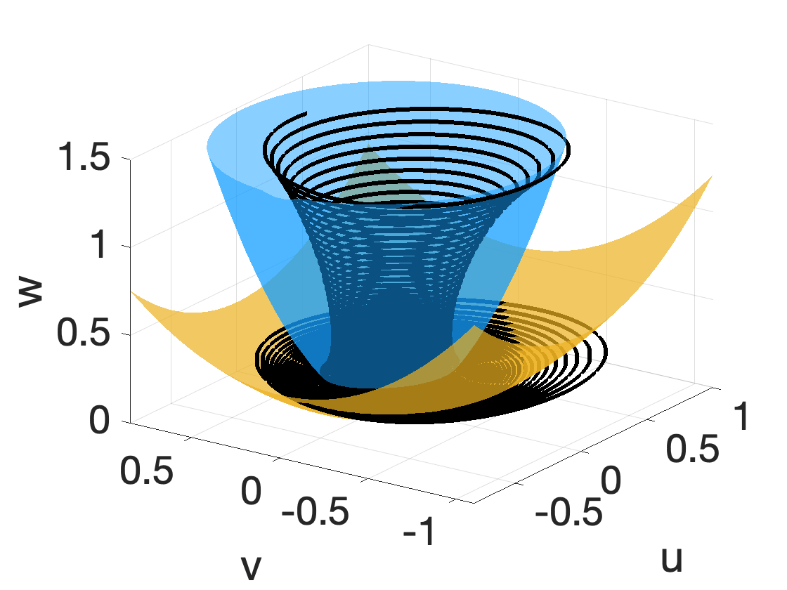
(a) IC = $(0.452,0.432,0.329)$

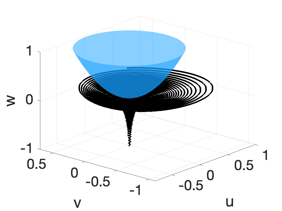
(b) IC=$(0.452,0.432,0.259)$

Figure 3. Behavior of trajectories of system (21) near the local stable manifold $W^{s}_{\textnormal{loc}}(q_{e})$ shown in golden for $\alpha=-0.04$ and the other parameter values are as in (52). In one case, (left panel) it enters into the funnel $\mathbb{R}^{3}\setminus\Omega_{\alpha}$, shown in deep sky blue, and in the other (right panel) it remains outside the funnel. For the purpose of visual clarity, $W^{s}_{\textnormal{loc}}(q_{e})$ is not drawn in the right panel.

3.2.1. Derivation and analysis of the averaged system

We start by integrating the third equation of (21) over an interval $[\tau,\tau+l]$ and use the fact that $\bar{w^{\prime}}=(\bar{w})^{\prime}$ to note that $\bar{w}(\tau)$ satisfies

(36) $$\frac{d\bar{w}}{d\tau}=\delta H_{3}\bar{w}+\frac{\delta}{2}H_{11}\bar{u^{2}}.$$

Solving (36) yields that

(37) $$\bar{w}(\tau)=\bar{w}(\tau_{0})e^{\delta H_{3}(\tau-\tau_{0})}+\frac{\delta H_{11}}{2}\int_{\tau_{0}}^{\tau}e^{\delta H_{3}(\tau-s)}\bar{u^{2}}(s)\ ds$$

for $\tau>\tau_{0}$, where $\tau_{0}\geq 0$ is an arbitrary chosen time. For a trajectory initiated near $W_{\mathrm{loc}}^{s}(q_{e})$, let $\{\tau_{i}\}_{i=1}^{N}$ be an increasing sequence of times where $u$ attains its local maxima such that $\{u(\tau_{i})\}_{i=1}^{N}$ is decreasing. Furthermore, assume that $w(\tau)$ has a decreasing envelope on the interval $[0,\tau_{N}]$ with $w(\tau)>0$. Let $I=[\tau_{1},\tau_{N}]$ and $p$ be the average period of oscillations of $u(\tau)$ in the interval $I$. Note that as long as the trajectory spirals inwards towards $q_{e}$, the dynamics of $u$ and $v$ can be approximated by (33), and thus $\bar{u^{2}}$, $\bar{v^{2}}$ will have the form $(a+c\sin(2\vartheta\tau)+d\cos(2\vartheta\tau))e^{b(\tau)\tau}+o(1)$ for some $a>0$, $c,d\approx 0$ and $b(\tau)<0$, a slowly varying function such that $b(\tau)\to\alpha\delta$ as $w(\tau)\to 0$. Here, $\vartheta\approx 2\pi/p$ and $a,b(\tau),c$, and $d$ depend on the initial conditions. For simplicity, we will assume that $b(\tau)=b_{2}$, where $b_{2}<0$ is such that $|b_{2}-\alpha\delta|=O(\delta^{4})$. We recall that $|\alpha|=O(\delta^{2})$, $u(0),v(0)=O(\sqrt{\delta})$ and $w(0)=O(\delta)$ here. Decomposing $\bar{u^{2}}(\tau)$ into the sum of its average and fluctuations from the mean, with the aid of (29) we can write $\bar{u^{2}}(\tau)=\bar{u^{2}}_{\textrm{est}}(\tau)+O(\delta^{2})$, where

(38) $$\bar{u^{2}}_{\textrm{est}}(\tau)=\bar{u^{2}}_{\textrm{base}}(\tau)+\bar{u^{2}}_{\textrm{osc}}(\tau)\ \textnormal{with}$$

(39) $$\bar{u^{2}}_{\textrm{base}}(\tau) = b_{1}e^{b_{2}(\tau-\tau_{1})},$$

$$\bar{u^{2}}_{\textrm{osc}}(\tau) = e^{b_{2}(\tau-\tau_{1})}\Big{(}\gamma_{1}\sin(2\vartheta(\tau-\tau_{1}))+\gamma_{2}\cos(2\vartheta(\tau-\tau_{1}))\Big{)},$$

$$b_{1} = \frac{A^{2}(1-e^{-pb_{2}})}{2pb_{2}}=O(\delta),\ b_{2}=\alpha\delta+O(\delta^{4}),\ \textrm{and}\ \gamma_{1},\gamma_{2}=O(\delta^{4}).$$

Remark 3.1.

The approximation of the decay function $b(\tau)$ by a constant $b_{2}$ is also valid for $\tau>\tau_{N}$ as long as the solution spirals inwards and stays in the vicinity of the $\{w=0\}$ plane. Therefore, the expressions in (38) and (39) are also valid beyond $\tau_{N}$.

In the following, we will ignore the contribution from $\bar{u^{2}}_{\textrm{osc}}(\tau)=O(\delta^{4})$ and only consider the effect of $\bar{u^{2}}_{\textrm{base}}(\tau)$, which represents the base value about which $\bar{u^{2}}(\tau)$ oscillates in $I$. Using the form of $\bar{u^{2}}_{\textrm{base}}(\tau)$ in (39) and choosing $\tau_{0}=\tau_{1}$, $l=p$, we then have from (37) that $\bar{w}=\bar{w}_{\textrm{base}}+O(\delta^{2})$, where

(40) $$\bar{w}_{\textrm{base}}(\tau)=\Big{(}\bar{w}(\tau_{1})-\frac{\delta H_{11}b_{1}}{2(b_{2}-\delta H_{3})}\Big{)}e^{\delta H_{3}(\tau-\tau_{1})}+\frac{\delta H_{11}b_{1}}{2(b_{2}-\delta H_{3})}e^{b_{2}(\tau-\tau_{1})}.$$

We also note that as long as $w(\tau)=O(\delta)$ and $u^{2}(\tau),v^{2}(\tau)=O(\delta)$, we have from (21) that $w^{\prime}(\tau)=O(\delta^{2})$. Hence, it follows from the Mean Value Theorem that $w(\tau)-\bar{w}(\tau)=\frac{1}{l}\int_{\tau}^{\tau+l}(w(\tau)-w(s))\ ds\leq\frac{l}{2}{\sup}_{I}|w^{\prime}|=O(\delta^{2})$ and thus $w(\tau)-\bar{w}_{\textrm{base}}(\tau)=O(\delta^{2})$. Given a solution $(u(\tau),v(\tau),w(\tau))$ of system (21) such that $|u(\tau)|$ has an initial decreasing envelope with $\bar{u^{2}}_{\textrm{base}}(\tau)$ satisfying (39), we will find a sufficient set of conditions on $\bar{w}(\tau_{1})$ which will determine the long-term behavior of the solution as stated in the next theorem.

Theorem 3.2.

Assume that $F_{13}>0$, $F_{111}<0$, $H_{3}>0$, $H_{11}<0$ such that $l_{1}(0)>0$ in (23) holds. Suppose $(u(\tau),v(\tau),w(\tau))$ is a solution of system (21) with initial values $(u_{0},v_{0},w_{0})$ such that $u_{0},v_{0}=O(\sqrt{\delta})$, $w_{0}=O(\delta)$ and $0<w_{0}<-\alpha/F_{13}$. Let $\{\tau_{i}\}_{i=1}^{N}$ be an increasing sequence of locations of relative maxima of $u(\tau)$ such that $\{u(\tau_{i})\}_{i=1}^{N}$ is decreasing, $(u(\tau),v(\tau),w(\tau))\in\Omega_{\alpha}$ for all $\tau\in[0,\tau_{N}]$, and $w(\tau)$ has a decreasing envelope on $[0,\tau_{N}]$ with $w({\tau}_{N})>0$. Then for $\alpha<0$ with $|\alpha|=O(\delta^{2})$ and $\delta>0$ sufficiently small, system (8) approaches $\Gamma_{\alpha}$ as $\tau\to\infty$ if

(41) $$\frac{\delta H_{11}b_{1}}{2(b_{2}-\delta H_{3})}+\delta^{2}<\bar{w}(\tau_{1})<-\frac{H_{11}b_{1}}{2H_{3}},$$

where

(42) $$b_{1} = \frac{A^{2}\vartheta}{4\pi b_{2}}(1-e^{\frac{-2\pi b_{2}}{\vartheta}}),\ b_{2}=\alpha\delta+O(\delta^{4})$$

with

(43) $$A = \frac{1}{\vartheta}\sqrt{u_{0}^{2}+u_{0}v_{0}b_{2}+v_{0}^{2}},\ \vartheta=\sqrt{1-\frac{\alpha^{2}\delta^{2}}{4}+O(\delta^{3})}.$$

On the other hand, if $\bar{w}(\tau_{1})<\frac{\delta H_{11}b_{1}e^{b_{2}\tau_{1}}}{2(b_{2}-\delta H_{3})}$, then $(u(\tau),v(\tau),w(\tau))\to(0,0,-\infty)$ as $\tau\to\infty$.

To prove the theorem, we will need a couple of lemmas.

Lemma 3.1.

Suppose the assumptions of Theorem 3.2 hold and $(u(\tau),v(\tau),w(\tau))$ is a solution of system (21) that satisfies condition (41). Then $w(\tau)$ attains its global minimum at some ${\tau}_{\mathrm{min}}>\tau_{N}$ and there exist $\tau_{a},\tau_{b}>{\tau}_{\mathrm{min}}$ such that
$(u(\tau),v(\tau),w(\tau))\in\mathbb{R}^{3}\setminus\Omega_{\alpha}$ for all $\tau\in[\tau_{a},\tau_{b}]$.

Proof.

Let $\{\tau_{i}\}_{i=1}^{M}$ be an increasing sequence of locations of relative maxima of $u(\tau)$, where $M>N$ is the largest integer such that $\{u(\tau_{i})\}_{i=1}^{M}$ is decreasing with $w(\tau)>0$ on $[0,\tau_{M}]$. By Remark 3.1, the expression for $\bar{u^{2}}_{\textrm{est}}(\tau)$ defined by (38)-(39) holds up to $O(\delta^{2})$ for all $\tau\in[\tau_{1},\tau_{M}]$. By our assumption, $w(\tau)$ has a decreasing envelope for all $\tau\in[\tau_{1},\tau_{N}]$, so $\bar{w}(\tau)$ also has a decreasing envelope on this interval. Estimating $\bar{w}(\tau)$ by $\bar{w}_{\textrm{base}}(\tau)$, where $\bar{w}_{\textrm{base}}(\tau)$ is defined by (40), it can be easily verified that $\bar{w}_{\textrm{base}}(\tau)$ has a unique critical point at $\tau=\bar{\tau}_{m}$, where

$$\bar{\tau}_{m}=\frac{1}{\delta H_{3}-b_{2}}\ln\Big{(}\frac{H_{11}b_{1}b_{2}e^{(\delta H_{3}-b_{2})\tau_{1}}}{H_{3}(2\bar{w}(\tau_{1})(\delta H_{3}-b_{2})+\delta H_{11}b_{1})}\Big{)}$$

if (41) holds. The critical point corresponds to a minimum of $\bar{w}_{\textrm{base}}(\tau)$ with

$$\bar{w}_{\textrm{base}}(\bar{\tau}_{m})=\frac{-H_{11}b_{1}}{2H_{3}}e^{b_{2}(\bar{\tau}_{m}-\tau_{1})}>0.$$

Since $\bar{w}(\tau)-\bar{w}_{\textrm{base}}(\tau)=O(\delta^{2})$ as long as $w(\tau)=O(\delta)$, it follows that $\bar{w}(\tau)$ and the lower envelope of $w(\tau)$ also attain their minima. Consequently, $w(\tau)$ attains its global minimum at $\tau={\tau}_{\mathrm{min}}$, where ${\tau}_{\mathrm{min}}={\bar{\tau}}_{m}+O(\delta^{2})$. Since by our assumption $0<w_{0}<-\alpha/F_{13}$, we must have $w({\tau}_{\mathrm{min}})<-\alpha/F_{13}$ as well, and therefore it follows from (33) that ${\tau}_{\mathrm{min}}<\tau_{M}$.

Next, we consider the relative position of $w(\tau)$ with respect to $-\frac{H_{11}}{2H_{3}}(u^{2}+v^{2})(\tau)$. By our assumption, $w(\tau)<-\frac{H_{11}}{2H_{3}}(u^{2}+v^{2})(\tau)$ for all $\tau\in[0,\tau_{N}]$. Let $\{t_{k}\}_{k=1}^{M}$ and $\{s_{k}\}_{k=1}^{M-1}$ be an increasing sequence of locations of relative maxima and minima of $v(\tau)$ in $I$ respectively with $t_{k}<\tau_{k}<s_{k}$. Since the trajectory is spiraling inwards, we have that $\{v(t_{k})\}_{k=1}^{M}$ and $\{v(s_{k})\}_{k=1}^{M-1}$ are decreasing and increasing respectively. Without loss of generality, we assume that $|v(t_{k})|\leq|v(s_{k})|$ for all $1\leq k\leq M-1$. With the aid of (21), we note that the zeros of $u(\tau)$ correspond to the critical points of $(u^{2}+v^{2})(\tau)$. Hence the relative maxima and minima of $(u^{2}+v^{2})(\tau)$ occur at $s_{k}$ and $t_{k}$ respectively with values $v^{2}(s_{k})$ and $v^{2}(t_{k})$ for all $k$. Denoting the local maxima and minima of $-\frac{H_{11}}{2H_{3}}(u^{2}+v^{2})(\tau)$ on the interval $[t_{k},s_{k}]$ by $M_{k}$ and $m_{k}$ respectively, we then have that $\{M_{k}\}_{k=1}^{M-1}$ and $\{m_{k}\}_{k=1}^{M-1}$ are both decreasing.

If $u_{\textrm{env}}(\tau)$ and $v_{\textrm{env}}(\tau)$ denote the upper envelopes of $u(\tau)$ and $v(\tau)$ respectively, we then have from (29) that up to $O(\delta^{2})$, $u_{\textrm{env}}(\tau)=Ae^{c_{2}(\tau-\tau_{1})}$ and $v_{\textrm{env}}(\tau)=Be^{c_{2}(\tau-\tau_{1})}$ for $\tau\in[\tau_{1},\tau_{M}]$, where $A$ is defined by (43) and

(44) $$B=\frac{A}{c_{2}^{2}+\vartheta^{2}},\ c_{2}=\frac{b_{2}}{2}=\frac{\alpha\delta}{2}+O(\delta^{4}).$$

We further note that if $w(\tau)\geq M_{i}$ on $[s_{i},t_{i+1}]$ for some $i$, where $s_{i}>{\tau}_{\mathrm{min}}$, then the trajectory is in the funnel, $\mathbb{R}^{3}\setminus\Omega_{\alpha}$ over the interval $[s_{i},t_{i+1}]$. The monotonic properties of $\{M_{k}\}_{k=1}^{M-1}$ and $\{m_{k}\}_{k=1}^{M-1}$, and the fact that $\bar{w}^{\prime}(\tau)>0$ for $\tau>{\tau}_{\mathrm{min}}$ will then imply that the trajectory is in the funnel over the interval $[s_{i},\tau_{M}]$.

To complete the proof of the lemma, we will show that there exist $\tau_{a},\tau_{b}>{\tau}_{\mathrm{min}}$ such that $w(\tau)>-\frac{H_{11}}{2H_{3}}(u^{2}+v^{2})(\tau)$ on $[\tau_{a},\tau_{b}]$. Since $(u^{2}+v^{2})(\tau)\leq(u_{\textrm{env}}^{2}(\tau)+v_{\textrm{env}}^{2}(\tau))$ and $|w(\tau)-\bar{w}_{\textrm{base}}(\tau)|=O(\delta^{2})$, it suffices to show that there exists some $\tau_{c}\in({\tau}_{\mathrm{min}},\tau_{M})$ such that $\bar{w}_{\textrm{base}}(\tau)>-\frac{H_{11}}{2H_{3}}(u_{\textrm{env}}^{2}(\tau)+v_{\textrm{env}}^{2}(\tau))$ for $\tau\in(\tau_{c},\tau_{M}]$. Choosing $\tau_{a}=s_{j}$, where $1<j<M$ is the smallest integer such that $s_{j}\leq\tau_{c}$ with $w(s_{j})>M_{j}$, and $\tau_{b}=\tau_{M}$ will then yield the result. To this end, we note from (40) that $\bar{w}_{\textrm{base}}(\tau)$ intersects with $\frac{-H_{11}}{2H_{3}}(u_{\textrm{env}}^{2}(\tau)+v_{\textrm{env}}^{2}(\tau))$ if $\frac{-H_{11}(A^{2}+B^{2})}{2H_{3}}>\frac{\delta H_{11}b_{1}}{2(b_{2}-\delta H_{3})}$. Using the relationships in (42) and (44), the above inequality simplifies to

(45) $$1+\frac{1}{c_{2}^{2}+\vartheta^{2}}>-\frac{1-e^{\frac{-4\pi c_{2}}{\vartheta}}}{\frac{8\pi c_{2}}{\vartheta}\Big{(}\frac{2c_{2}}{\delta H_{3}}-1\Big{)}}.$$

Since $c_{2}=O(\alpha\delta/2)$ and $\vartheta\approx 1$, it then follows that the left hand side of (45) is approximately equal to $2$, whereas the right hand side of (45) is less than $1/2$ for $\delta$ sufficiently small, and thus (45) holds. Let $\tau_{c}$ be the point of intersection of $\bar{w}_{\textrm{base}}(\tau)$ and $-\frac{H_{11}}{2H_{3}}(u_{\textrm{env}}^{2}(\tau)+v_{\textrm{env}}^{2}(\tau))$. Since $\bar{w}^{\prime}_{\textrm{base}}(\tau)<0$ on $[\tau_{1},\bar{\tau}_{m})$ and $b_{1}\approx A^{2}/2$, it follows from (36), (39) and (42) that for sufficiently small $\delta>0$,

$$\bar{w}_{\textrm{base}}(\tau)\leq\frac{-H_{11}}{2H_{3}}\bar{u^{2}}_{\textrm{base}}<\frac{-H_{11}}{2H_{3}}A^{2}<-\frac{H_{11}}{2H_{3}}(u_{\textrm{env}}^{2}(\tau)+v_{\textrm{env}}^{2}(\tau)\ \textnormal{on}\ [\tau_{1},\bar{\tau}_{m}].$$

Consequently, $\tau_{c}>\bar{\tau}_{m}=\tau_{\textrm{min}}+O(\delta^{2})$. The intersection of $\bar{w}_{\textrm{base}}(\tau)$ with
$-\frac{H_{11}}{2H_{3}}(u_{\textrm{env}}^{2}(\tau)+v_{\textrm{env}}^{2}(\tau))$ then implies that $\bar{w}_{\textrm{base}}(\tau)>-\frac{H_{11}}{2H_{3}}(u_{\textrm{env}}^{2}(\tau)+v_{\textrm{env}}^{2}(\tau))$ in $(\tau_{c},\tau_{M}]$, which completes the proof. ∎

Lemma 3.2.

Under the assumptions of Theorem 3.2, the set $\Omega_{\alpha}$ is positively invariant with respect to the solution $(u(\tau),v(\tau),w(\tau))$ of system (21) if $\bar{w}(\tau_{1})<\frac{\delta H_{11}b_{1}}{2(b_{2}-\delta H_{3})}$, where $b_{1}$ and $b_{2}$ are defined as in Theorem 3.2. Furthermore,
$(u(\tau),v(\tau),w(\tau))\to(0,0,-\infty)$ as $\tau\to\infty$.

Proof.

Let $\{\tau_{i}\}_{i=1}^{M}$ be an increasing sequence of locations of relative maxima of $u(\tau)$ such that $\{u(\tau_{i})\}_{i=1}^{M}$ is decreasing, where $M$ is some integer greater than $N$ to be chosen later. By Remark 3.1, we note that the expressions for $\bar{u^{2}}_{\textrm{est}}(\tau)$ and $\bar{w}_{\textrm{base}}(\tau)$ defined by (38) and (40) respectively, hold up to $O(\delta^{2})$ for all $\tau\in[\tau_{1},\tau_{M}]$. If $\bar{w}(\tau_{1})<\frac{\delta H_{11}b_{1}}{2(b_{2}-\delta H_{3})}$, then it follows from (40) that $\bar{w}_{\textrm{base}}(\tau)$ decreases and eventually becomes negative at $\tau=\tau_{e}$, where

$${\tau_{e}}=\frac{1}{\delta H_{3}-b_{2}}\ln\Big{(}\frac{\delta H_{11}b_{1}e^{(\delta H_{3}-b_{2})\tau_{1}}}{\delta H_{11}b_{2}e^{b_{2}\tau_{1}}+2\bar{w}(\tau_{1})(\delta H_{3}-b_{2})}\Big{)}.$$

Since $|w(\tau)-\bar{w}_{\textrm{base}}(\tau)|=O(\delta^{2})$ and $\bar{w}_{\textrm{base}}^{\prime}(\tau)<0$ for all $\tau\in[0,\tau_{M}]$, we must have that $w(\tau)$ also changes its sign near $\tau_{e}$. Let $\tilde{\tau}=\tau_{e}+o(1)$ be such that $w(\tilde{\tau})=0$. Choose $M$ large enough such that $\tilde{\tau}<\tau_{M}$. Since $q_{e}$ is unstable along the $w$-direction and $w^{\prime}(\tilde{\tau})=\frac{\delta}{2}H_{11}u^{2}(\tilde{\tau})\leq 0$ (follows from from (21)), we cannot have $w(\tau)=0$ for all $\tau\geq\tilde{\tau}$, thereby leading to $w(\tau)<0\leq-\frac{H_{11}}{2H_{3}}(u^{2}+v^{2})(\tau)$ for all $\tau>\tilde{\tau}$. Thus $(u(\tau),v(\tau),w(\tau))\in\Omega_{\alpha}$ for all $\tau>\tilde{\tau}$. It is also evident from (21) that $w^{\prime}(\tau)<\delta H_{3}w$ and therefore if $w(\bar{\tau})=-k$ for some $k>0$ and $\bar{\tau}>\tilde{\tau}$, then by Gronwall’s inequality, $w(\tau)<-ke^{\delta H_{3}(\tau-\bar{\tau})}\to-\infty$ as $\tau\to\infty$. Consequently, the fast variables $(u(\tau),v(\tau))$, governed by system (33), approach $(0,0)$ as $\tau\to\infty$.

Next, we will prove that $\Omega_{\alpha}$ is positively invariant with respect to
$(u(\tau),v(\tau),w(\tau))$ for all $\tau\geq 0$. Denoting the sequences of local minima and maxima of $-\frac{H_{11}}{2H_{3}}(u^{2}+v^{2})$ by $\{m_{k}\}_{k=1}^{M-1}$ and $\{M_{k}\}_{k=1}^{M-1}$ and their locations by $\{t_{k}\}_{k=1}^{M-1}$ and $\{s_{k}\}_{k=1}^{M-1}$ respectively with $t_{k}<\tau_{k}<s_{k}$, and recalling that $(u(\tau),v(\tau),w(\tau))\in\Omega_{\alpha}$ on $[0,\tau_{N}]$, we then have that $w(\tau)<m_{k}$ on the interval $[t_{k},t_{k+1})$ for all $1\leq k\leq N-1$. As in the proof of Lemma 3.1, we have that $m_{k}=-\frac{H_{11}}{2H_{3}}v^{2}(t_{k})=-\frac{H_{11}B^{2}}{2H_{3}}e^{b_{2}(t_{k}-\tau_{1})}$ up to $O(\delta^{2})$, where $B$ is defined by (44), and thus we have $\bar{w}_{\textrm{base}}(\tau)\approx w(\tau)<-\frac{H_{11}B^{2}}{2H_{3}}e^{b_{2}(\tau-\tau_{1})}$ on $[0,\tau_{N}]$, i.e.

(46) $$\frac{\delta H_{11}b_{1}}{2(b_{2}-\delta H_{3})}<-\frac{H_{11}B^{2}}{2H_{3}}.$$

Since by our assumption $\bar{w}(\tau_{1})<\frac{\delta H_{11}b_{1}}{2(b_{2}-\delta H_{3})}$, we have from (40) in combination with (46) that $\bar{w}_{\textrm{base}}(\tau)<m_{k}$ on $[t_{k},t_{k+1})$ for all $1\leq k\leq M-1$, i.e. $\bar{w}_{\textrm{base}}(\tau)<-\frac{H_{11}}{2H_{3}}(u^{2}+v^{2})(\tau)$ for all $\tau\in[0,\tau_{M}]$. Finally, since $w(\tau)=\bar{w}_{\textrm{base}}(\tau)+O(\delta^{2})$, we can conclude that the solution is in $\Omega_{\alpha}$ for all $\tau\in[0,\tau_{M}]$. Combining this with the fact that $(u(\tau),v(\tau),w(\tau))\in\Omega_{\alpha}$ for all $\tau>\tilde{\tau}$ proves the lemma. ∎

Proof of Theorem 3.2: Lemma 3.1 implies that a solution of (8) initiated in $\Omega_{\alpha}$ enters into the funnel, $\mathbb{R}^{3}\setminus\Omega_{\alpha}$, and remains inside it for all $\tau\in[\tau_{a},\tau_{b}]$ if (41) holds. Furthermore, it follows from (33) that as long as the trajectory spirals inward, it remains inside the funnel; in particular this occurs for all $\tau>\tau_{a}$ such that $w(\tau)<-\alpha/F_{13}$. We also note from property (Q5) that the basin of attraction of $\Gamma_{\alpha}$ must contain the set $\mathcal{B}:=\{(u,v,w)\in[-\delta,\delta]\times[-\delta,\delta]\times(0,-\alpha/F_{13}]:w\geq\Theta(u,v,\delta)-\delta^{2}\}\cap\{w>-H_{11}/(2H_{3})u^{2}\}$ for sufficiently small $\delta>0$, where $\Theta(u,v,\delta)$ is defined by (30). Since $\mathbb{R}^{3}\setminus\Omega_{\alpha}\cap\{w<-\alpha/F_{13}\}\subset\mathcal{B}$ for all $\delta>0$ sufficiently small, hence the flow restricted to $\{(u,v,w)\in\mathbb{R}^{3}\setminus\Omega_{\alpha}:0<w\leq-\alpha/F_{13}\}$ must approach the attractor $\Gamma_{\alpha}$ as $\tau\to\infty$, which proves the first part of Theorem 3.2. The second part of Theorem 3.2 follows directly from Lemma 3.2.

4. Early warning signals

In the previous section, we obtained a set of sufficient conditions on $\bar{w}(\tau_{1})$ to predict the asymptotic behavior of a trajectory as it approaches the equilibrium $q_{e}$. In this section, we focus on finding a method of predicting long-term behaviors of trajectories as early as possible during their journeys towards $q_{e}$ in the same parameter regime considered in Theorem 3.2. The significance of the method lies in finding the shortest time interval over which we can predict a forthcoming sign change in $w(\tau)$ when a trajectory fails to enter into the funnel $\mathbb{R}^{3}\setminus\Omega_{\alpha}$ as it approaches $q_{e}$.

Due to the difference in timescales between the frequency and the amplitude of oscillations of $u(\tau)$, we can choose the initial conditions in such a way that there exist at least $N\gg 1$ oscillations before the amplitude of $u(\tau)$ decays by a factor of $e$. Indeed, we note from (29) that as a solution of (8) approaches $q_{e}$, the amplitude of $u(\tau)$ decays exponentially with the decay function $b(\tau)/2\approx\alpha\delta/2$, while the frequency of its oscillations $\vartheta\approx 1-\frac{1}{8}\alpha^{2}\delta^{2}\approx 1$ for sufficiently small $\delta>0$, hence one can choose $(u_{0},v_{0},w_{0})$ such that $\tau_{N}>\frac{\vartheta}{2\pi|b(\tau_{N})|}$, where $\tau_{i}$, $i=1,2,\ldots,N,\ldots$ are the locations of relative maxima of $u(\tau)$. We now define a sequence of intervals $I_{i}=[\tau_{1},\tau_{k+i}]$, $i=1,2\ldots N-k$ such that each interval contains at least $k$ oscillations of $u$, where $k\ll N$. The goal is to find the smallest interval $I_{i}$ (and therefore obtain the shortest time) on which a forthcoming population collapse can be accurately predicted.

To this end, let $l_{i}$ be the average period of oscillations of $u(\tau)$ in the interval $I_{i}$, i.e. $l_{i}=\frac{1}{k+i}\sum_{j=1}^{k+i-1}(\tau_{j+1}-\tau_{j})$. On each interval $I_{i}$, we will approximate $\bar{u^{2}}$ by $\bar{u^{2}_{i}}_{\textrm{est}}$, where $\bar{u^{2}_{i}}_{\textrm{est}}(\tau)=\bar{u^{2}_{i}}_{\textrm{base}}(\tau)+\bar{u^{2}_{i}}_{\textrm{osc}}(\tau)$ with

$$\bar{u^{2}_{i}}_{\textrm{base}}(\tau)=k^{i}_{1}e^{k^{i}_{2}(\tau-\tau_{1})},\ \bar{u^{2}_{i}}_{\textrm{osc}}(\tau)=e^{k^{i}_{2}(\tau-\tau_{1})}\Big{(}\gamma^{i}_{1}\sin\Big{(}\frac{\pi(\tau-\tau_{1})}{l_{i}}\Big{)}+\gamma^{i}_{2}\cos\Big{(}\frac{\pi(\tau-\tau_{1})}{l_{i}}\Big{)}\Big{)},$$

(47) $$k^{i}_{1}=\frac{1}{\vartheta}\sqrt{u^{2}(\tau_{1})+u(\tau_{1})v(\tau_{1})k^{i}_{2}+v^{2}(\tau_{1})},\ k^{i}_{2}=O(\alpha\delta)\ \textnormal{and}\ \gamma^{i}_{1},\gamma^{i}_{2}=O(\delta^{4}).$$

Here $0<k_{1}^{i}=O(\delta)$ and $k_{2}^{i}<0$. We will assume that $\{k_{1}^{i}\}_{i=1}^{N-k}$ and $\{k_{2}^{i}\}_{i=1}^{N-k}$ are monotonically decreasing and increasing respectively. Furthermore, we will assume that $\{l_{i}\}_{i=1}^{N-k}$ is nearly constant with $|l_{i+1}-l_{i}|=O(\delta^{4})$. As in Section 3, we will ignore the contribution from $\bar{u^{2}_{i}}_{\textrm{osc}}(\tau)=O(\delta^{4})$ and only consider the effect of $\bar{u^{2}_{i}}_{\textrm{base}}(\tau)$, which represents the base value about which $\bar{u^{2}}(\tau)$ oscillates in $I_{i}$. Letting $l=l_{i}$ in (35), we consider the moving average of $w$ restricted to $I_{i}$. Using the above form of $\bar{u^{2}_{i}}_{\textrm{base}}(\tau)$, we then have from (37) that

(48) $$\bar{w}^{i}_{\textrm{base}}(\tau)=\Big{(}\bar{w}(\tau_{1})-\frac{\delta H_{11}k^{i}_{1}}{2(k^{i}_{2}-\delta H_{3})}\Big{)}e^{\delta H_{3}(\tau-\tau_{1})}+\frac{\delta H_{11}k^{i}_{1}}{2(k^{i}_{2}-\delta H_{3})}e^{k^{i}_{2}(\tau-\tau_{1})},$$

where $\bar{w}^{i}_{\textrm{base}}(\tau)$ is an approximation of $\bar{w}(\tau)$ with $|\bar{w}(\tau)-\bar{w}^{i}_{\textrm{base}}(\tau)|=o(1)$ on the interval $I_{i}$. For each $i$ between $1$ and $N-k$, we define a critical curve $\bar{w}^{i}_{\textrm{crit}}(\tau)$ by

(49) $$\bar{w}^{i}_{\textrm{crit}}(\tau)=\frac{\delta H_{11}k^{i}_{1}e^{k^{i}_{2}(\tau-\tau_{1})}}{2(k^{i}_{2}-\delta H_{3})},\ \tau\in I_{i}.$$

We will examine the behavior of $\bar{w}^{i}_{\textrm{base}}(\tau)$ relative to its position with respect to $\bar{w}^{i}_{\textrm{crit}}(\tau)$ as stated in the next two propositions.

Proposition 4.1.

Assume that $F_{13}>0$, $F_{111}<0$, $H_{3}>0$, $H_{11}<0$ are such that $l_{1}(0)>0$ in (23) holds and $O(\delta^{2})=\alpha<0$. Suppose $(u(\tau),v(\tau),w(\tau))$ is a solution of system (21) with initial values $(u_{0},v_{0},w_{0})$ satisfying $u_{0},v_{0}=O(\sqrt{\delta})$ and $0<w_{0}=O(\delta)$. Let $\{I_{i}\}_{i=1}^{N-k}$ be a sequence of nested intervals defined by $I_{i}=[\tau_{1},\tau_{k+i}]$, where $\{\tau_{i}\}_{i=1}^{N-k}$ is an increasing sequence of locations of relative maxima of $u(\tau)$ such that $\{u(\tau_{i})\}_{i=1}^{N}$ is decreasing and $k\ll N$ is a fixed integer greater than $4$ with $N=O(\frac{k}{\delta})$. Suppose $\{k_{1}^{i}\}_{i=1}^{N-k}$ and $\{k_{2}^{i}\}_{i=1}^{N-k}$, defined by (47), are respectively decreasing and increasing sequences of real numbers such that $\bar{u^{2}}(\tau)=k_{1}^{i}e^{k_{2}^{i}(\tau-\tau_{1})}+o(1)$ on $I_{i}$. Then $w(\tau)$ attains its global minimum in $I_{N-k}$ if

$$\bar{w}(\tau) > \bar{w}^{1}_{\textrm{crit}}(\tau)\ \textrm{on}\ I_{1}\ \textrm{and}$$

(50) $$\bar{w}(\tau) > \bar{w}^{i}_{\textrm{crit}}(\tau)\ \textrm{on}\ I_{i}\setminus I_{i-1}\ \textrm{for all}\ 2\leq i\leq N-k,$$

where $\bar{w}^{i}_{\textrm{crit}}(\tau)$ is defined by (49).

Proof.

Since $\bar{w}(\tau)=\bar{w}^{i}_{\textrm{base}}(\tau)+o(1)$, it follows that $\bar{w}^{i}_{\textrm{base}}(\tau)$ also satisfies (50) if $\bar{w}(\tau)$ satisfies condition (50). It can be easily verified from (48) that if $\bar{w}^{i}_{\textrm{base}}(\tau)>\bar{w}^{i}_{\textrm{crit}}(\tau)$ then $\bar{w}^{i}_{\textrm{base}}(\tau)$ attains a minimum at $\tau=\bar{\tau}_{i}$, where

$$\bar{\tau}_{i}=\frac{1}{\delta H_{3}-k^{i}_{2}}\ln\Big{(}\frac{H_{11}k^{i}_{1}k^{i}_{2}e^{(\delta H_{3}-k^{i}_{2})\tau_{1}}}{H_{3}(2\bar{w}(\tau_{1})(\delta H_{3}-k^{i}_{2})+\delta H_{11}k^{i}_{1})}\Big{)}.$$

Let $M$ be the smallest integer between $1$ and $N-k$ such that $\bar{\tau}_{M}\in I_{M}$. Then $\bar{w}$ will also attain its minimum near $\bar{\tau}_{M}$. Consequently, $w$ will attain its global minimum near $\bar{\tau}_{M}\in I_{N-k}$. ∎

In the next proposition, we will show that the trajectory continues to spiral down and crosses the $\{w=0\}$ plane if $\bar{w}^{i}_{\textrm{base}}(\tau)$ is below $\bar{w}^{i}_{\textrm{crit}}(\tau)$ on $I_{i}$ for some $i$.

Proposition 4.2.

Let $\{I_{i}\}_{i=1}^{N-k}$ be a sequence of nested intervals and $\{k^{i}_{1}\}_{i=1}^{N-k}$, $\{k^{i}_{2}\}_{i=1}^{N-k}$ be sequences of real numbers as defined in Proposition 4.1. Then there exists $\tilde{\tau}_{e}\in I_{N-k}$ such that $w(\tilde{\tau}_{e})=0$ with $w^{\prime}(\tilde{\tau}_{e})<0$ if $\bar{w}(\tau)<\bar{w}^{i_{0}}_{\textrm{crit}}(\tau)$ on $({\tilde{\tau}}_{i_{0}},\tau_{k+i_{0}}]$ for some $1\leq i_{0}\leq N-k$ and ${\tilde{\tau}}_{i_{0}}\in I_{i_{0}}$, where $\bar{w}^{i}_{\textrm{crit}}(\tau)$ is defined by (49).

Proof.

We first note that the monotonic properties of $\{k_{1}^{i}\}$ and $\{k_{2}^{i}\}$ imply that $\bar{w}^{i}_{\textrm{crit}}(\tau)<\bar{w}^{i+1}_{\textrm{crit}}(\tau)$ on $I_{i}$. Moreover, if $\bar{w}^{i}_{\textrm{base}}(\tau)<\bar{w}^{i}_{\textrm{crit}}(\tau)$ for some $i$, then it follows from (48) that $\bar{w}^{i}_{\textrm{base}}(\tau)$ decreases and eventually becomes negative at $\tau=\tilde{\tau}_{i}$, where

(51) $$\tilde{\tau}_{i}=\frac{1}{\delta H_{3}-k^{i}_{2}}\ln\Big{(}\frac{\delta H_{11}k^{i}_{1}e^{(\delta H_{3}-k^{i}_{2})\tau_{i}}}{\delta H_{11}k^{i}_{1}+2\bar{w}(\tau_{1})(\delta H_{3}-k^{i}_{2})}\Big{)}.$$

If there exists some point ${\tilde{\tau}}_{i_{0}}\in I_{i_{0}}$ such that $\bar{w}(\tau)<\bar{w}^{i_{0}}_{\textrm{crit}}(\tau)$ on $({\tilde{\tau}}_{i_{0}},\tau_{k+i_{0}}]$ for some $1\leq i_{0}\leq N-k$, then the monotonicity of the family $\{\bar{w}^{i}_{\textrm{crit}}(\tau)\}_{i=1}^{N-k}$ yields that $\bar{w}(\tau)<\bar{w}^{i}_{\textrm{crit}}(\tau)$ on $({\tilde{\tau}}_{i_{0}},\tau_{k+i}]$ for all $i\geq i_{0}$. Since $|\bar{w}-\bar{w}^{i}_{\textrm{base}}|=o(1)$, there exists an integer $j\geq i_{0}$ such that $\bar{w}^{j}_{\textrm{base}}(\tau)<\bar{w}^{j}_{\textrm{crit}}(\tau)$ with $\bar{w}^{j}_{\textrm{base}}(\tilde{\tau}_{j})=0$ and $\bar{w}^{j}_{\textrm{base}}(\tau)<0$ for $\tau>\tilde{\tau}_{j}$, where $\tilde{\tau}_{j}\in I_{j}$ is defined by (51). Thus $\bar{w}(\tau)$ and $w(\tau)$ change their signs at $\tilde{\tau}_{e}=\tilde{\tau}_{j}+o(1)$ and remain negative thereafter, thereby proving the proposition. ∎

Note that Propositions 4.1 and 4.2 are complementary to each other as a solution passing through a vicinity of $q_{e}$ either meets the conditions in Proposition 4.1 or Proposition 4.2. To see how the method plays out, we start by approximating $\bar{u^{2}}(\tau)$ by $\bar{u^{2}_{1}}_{\textrm{base}}(\tau)$ on the interval $I_{1}$ and examine the position of $\bar{w}(\tau)$ with respect to $\bar{w}^{1}_{\textrm{crit}}(\tau)$. If $\bar{w}(\tau)$ meets the condition in Proposition 4.2, then we obtain an early warning signal of a sign change in $w(\tau)$. However, if that is not the case, we consider $I_{2}$ and use $\bar{u^{2}_{2}}_{\textrm{base}}(\tau)$ as a new approximation to $\bar{u^{2}}(\tau)$ on the interval $I_{2}$. We again examine the position of $\bar{w}(\tau)$ with respect to $\bar{w}^{2}_{\textrm{crit}}(\tau)$ and check if $\bar{w}(\tau)$ meets the condition in Proposition 4.2. If not, we subsequently repeat the process and apply the technique on the intervals $I_{i},3\leq i\leq N-k$ until $\bar{w}$ meets the condition in Proposition 4.2. If it fails, then (50) must hold, in which case $\bar{w}$ attains its minimum.

5. Numerical results

5.1. Behavior of system (16) near the singular Hopf bifurcation

We return to system (16) and compute the coefficients of the normal form (21) near the singular Hopf bifurcation. Treating $h$ as the input parameter and the other parameter values as in (17), the coefficients of the normal form (21) are

(52) $$\delta\approx 0.2504,\ F_{13}\approx 0.1173,\ F_{111}\approx-0.8663,\ H_{3}\approx 0.0377,\ H_{11}\approx-0.1691,$$

with $\alpha(h)=-145.8265h+38.589$ being the varying parameter. The eigenvalues of the variational matrix of system (21) at the equilibrium $q_{e}=(0,0,0)$ (which corresponds to the coexistence equilibrium $E^{*}$ of system (16)) are $\lambda_{1}\approx 0.00943$ and a complex pair $\lambda_{2,3}$ with $\textnormal{Re}(\lambda_{2,3})<0$ if $-3.997<\alpha<0$. A subcritical Hopf bifurcation occurs at $\alpha=\alpha_{H}=0$ (which corresponds to $H_{2}\approx 0.2646$ in system (16)), where the first Lyapunov coefficient $l_{1}(0)\approx 0.0934>0$. In an immediate neighborhood of the Hopf bifurcation, system (21) undergoes a subcritical torus bifurcation at $\alpha=-0.011$ (corresponding to $TR\approx 0.2647$ in system (16)), stabilizing the family of cycles $\Gamma^{\alpha}$ born at $\alpha=0$.

In a vicinity of $\alpha=-0.011$, system (21) exhibits bistability between $\Gamma^{\alpha}$ and $(0,0,-\infty)$ as shown in 3. In both cases, $u(\tau)$ and $v(\tau)$ exhibit very similar oscillatory patterns, however $w(\tau)$ attains a global minimum in one case, while in the other, it fails to attain a minimum and becomes negative. In 4, we plot the time series of $\bar{u^{2}}(\tau)$, $\bar{w}(\tau)$ along with the approximating functions $\bar{u^{2}}_{\textrm{est}}(\tau)$ and $\bar{w}_{\textrm{base}}(\tau)$ respectively, where $\bar{u^{2}}_{\textrm{est}}(\tau)$ and $\bar{w}_{\textrm{base}}(\tau)$ are defined by (38) and (40) respectively. Note that the approximating curves lie very close to the actual curves uniformly over the time interval under consideration. By Theorem 3.2, $\bar{w}_{\textrm{base}}(\tau)$ attains a minimum if it satisfies condition (41) as shown in figure 5a. On the other hand, if $\bar{w}(\tau_{1})<\frac{\delta H_{11}b_{1}e^{b_{2}\tau_{1}}}{2(b_{2}-\delta H_{3})}$, $\bar{w}_{\textrm{base}}(\tau)$ eventually becomes negative as shown in figure 5b.

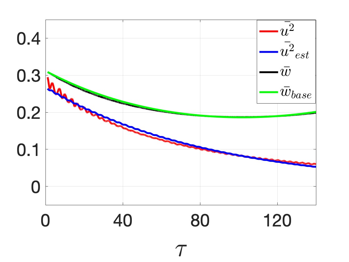
(a) IC = $(0.452,0.432,0.329)$

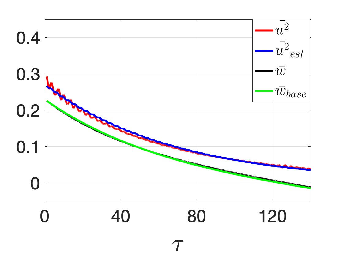
(b) IC=$(0.452,0.432,0.259)$

Figure 4. Graphs of $\bar{u^{2}}(\tau)$, $\bar{w}(\tau)$ and their approximations by $\bar{u^{2}}_{\textrm{est}}(\tau)$ and $\bar{w}_{\textrm{base}}(\tau)$ respectively for the same parameter values and initial conditions as in figure 3.

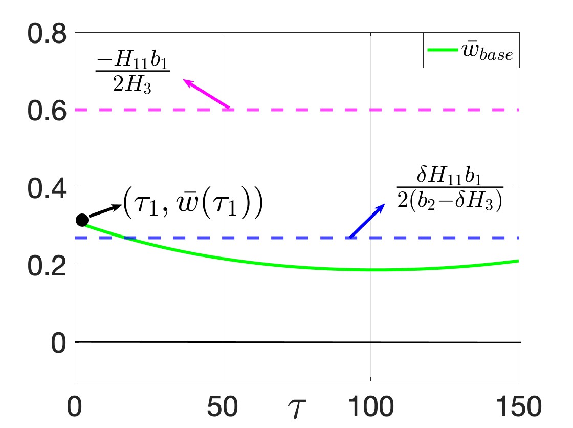
(a)

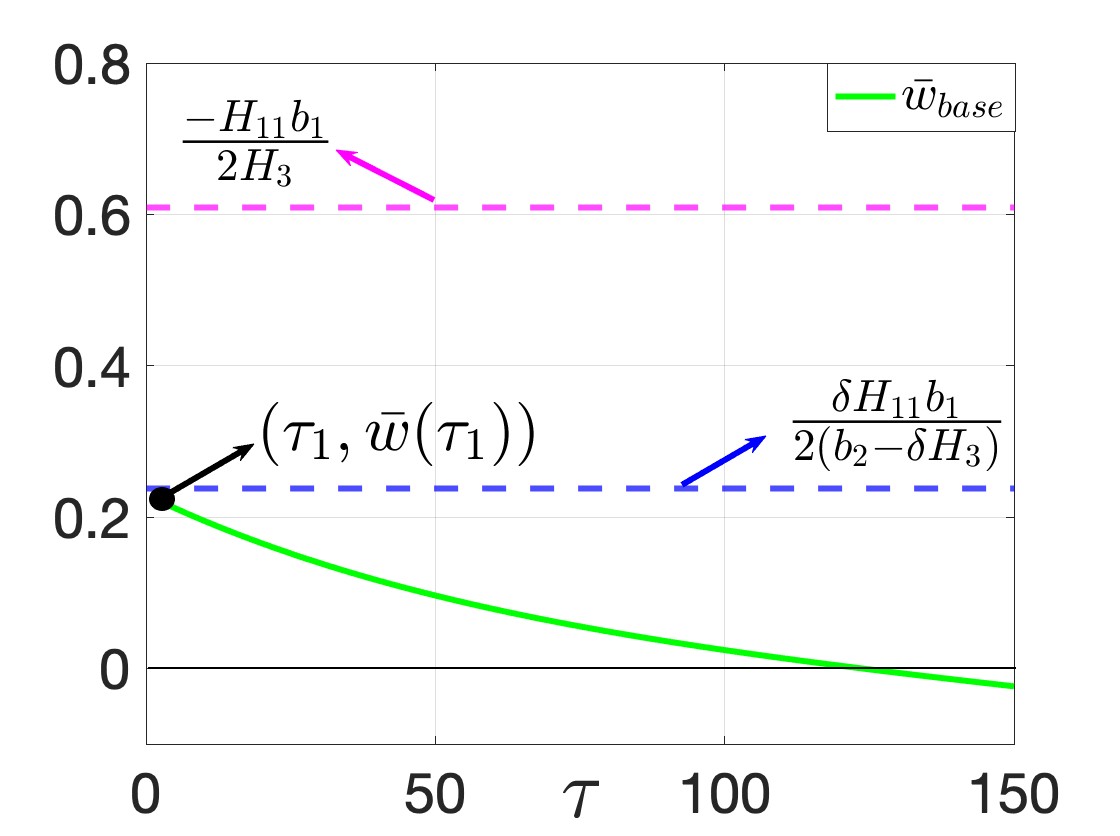
(b)

Figure 5. Behavior of $\bar{w}_{\textrm{base}}(\tau)$ for two different initial values as in 4. In both cases, $N=18$ oscillations were chosen. (a) Here $\tau_{1}=1.094$, $\tau_{N}=109.2$, $b_{1}=0.2799$ and $b_{2}=-0.0128$. (b) Here $\tau_{1}=1.0784$, $\tau_{N}=109.04$, $b_{1}=0.2799$ and $b_{2}=-0.0156$.

5.2. Analysis of the time series in figure 1

Finally, we consider the time series in figure 1. We first recall that the initial conditions for both solutions lie in a close neighborhood of $W^{s}(E^{*})$ and are in $\Sigma^{+}$, where $\Sigma^{+}$ is the upper-half space containing the limit cycle $\Gamma$ of system (16). We next note that the tangent plane $\Sigma$ in system (16) corresponds to $\{w=0\}$ in system (21); the limit cycle $\Gamma$ and the boundary equilibrium point $E_{xz}$ lie on the opposite sides of $\{w=0\}$. We now use the transformations given in the Appendix to map $(x,y,z)$ to $(u,v,w)$ and plot the solutions in their normal form with respect to the slow time variable $s$, as shown in figure 6. We also draw $\Sigma$ and the inverse images of $W^{s}_{\mathrm{loc}}(q_{e})$ (the expression in (30) is used to compute $W^{s}_{\mathrm{loc}}(E^{*})$) and the funnel $\mathbb{R}^{3}\setminus\Omega_{\alpha}$ in the $xyz$-coordinates with the phase spaces of the trajectories corresponding to figure 1 superimposed on them as shown in figure 7. As expected from the analysis of system (21), figure 7 shows that the solution associated with figure 1(a) enters into the funnel and approaches $\Gamma$, while the solution corresponding to figure 1(b) always remains outside the funnel, and eventually approaches the boundary equilibrium state $E_{xz}$.

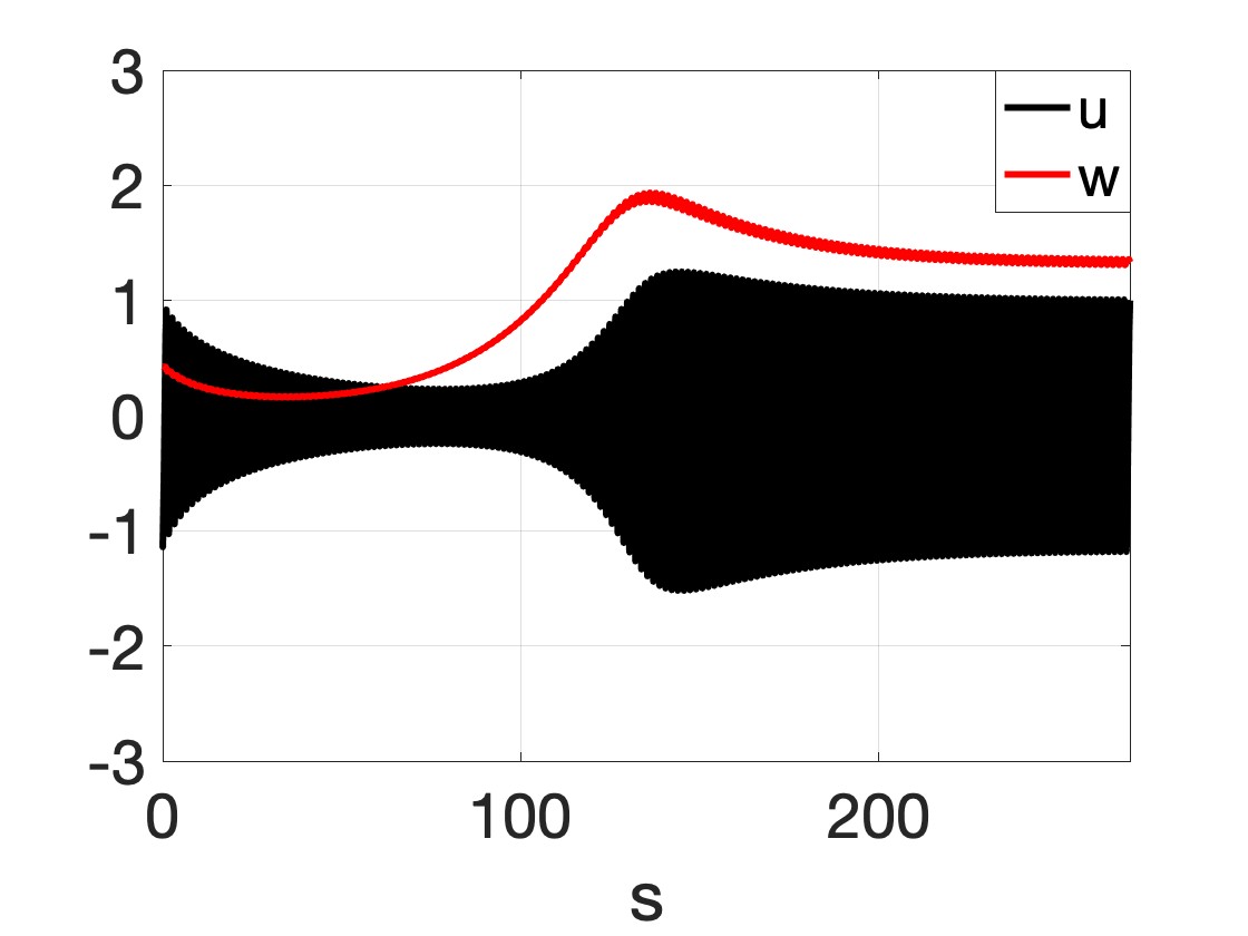
(a)

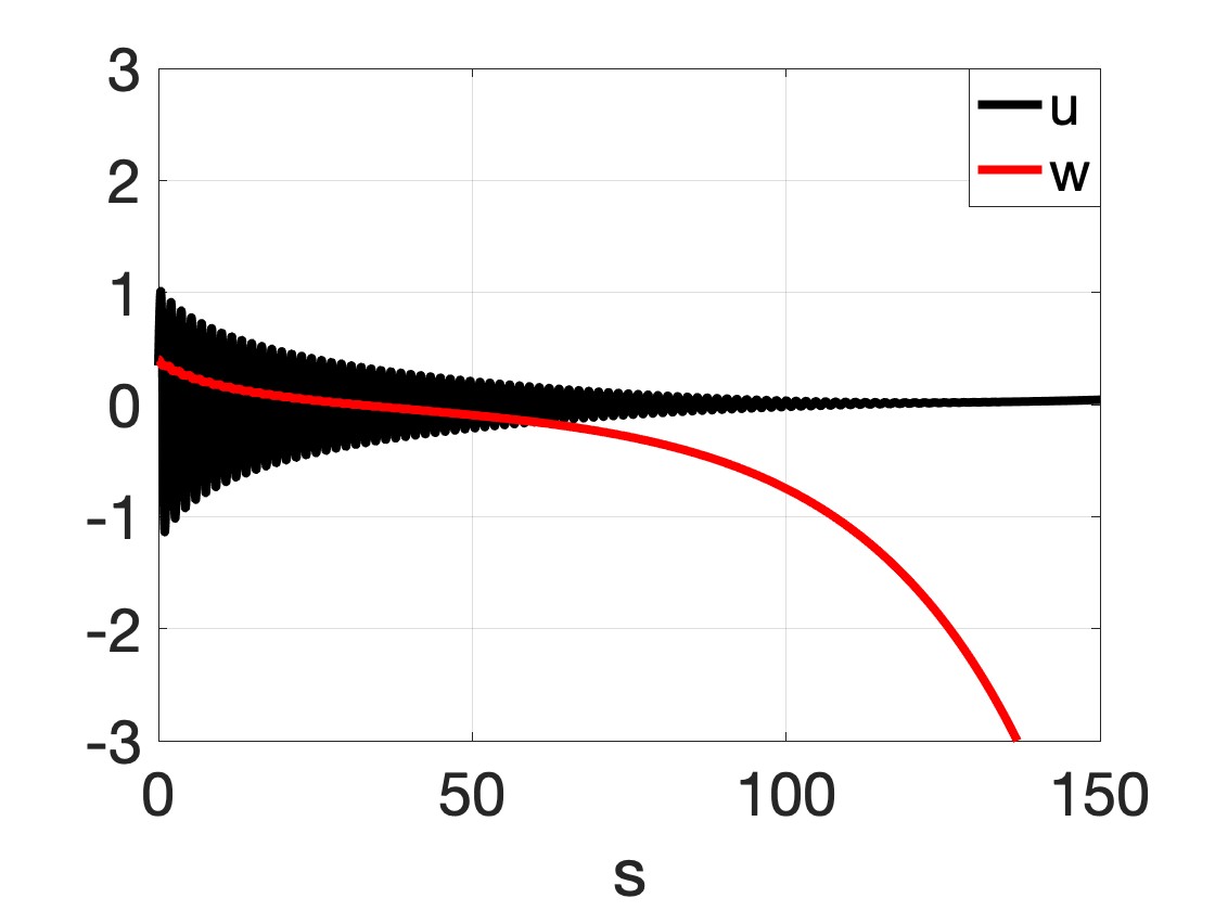
(b)

Figure 6. Time series of $x(s)$, $y(s)$ and $z(s)$ in figure 1 in terms of the normal form variables $u(s)$ and $w(s)$. The left panel corresponds to figure 1(a) and the right panel to figure 1(b).

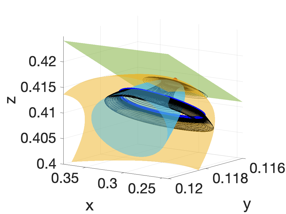
(a) IC: $(0.2785,0.1181,0.4164)\in\Sigma^{+}$

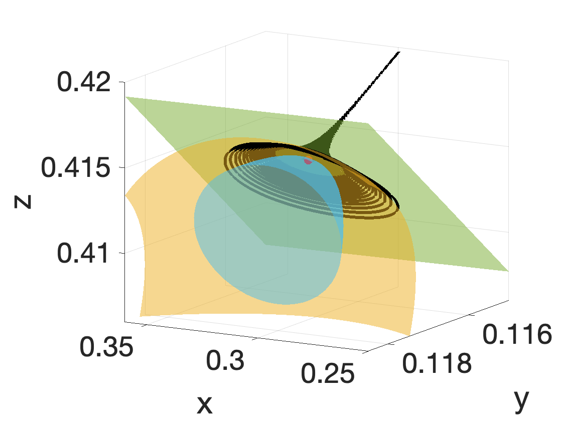
(b) IC: $(0.2831,0.1184,0.417)\in\Sigma^{+}$

Figure 7. Phase spaces of the solutions in figure 1 approaching $\Gamma$ (in blue) or $E_{xz}=(0.357,0,0.615)$. Also shown are $E^{*}$ (red dot), $W^{s}_{\mathrm{loc}}(E^{*})$ (golden surface), $\Sigma$ (olive green plane) and the inverse image of the funnel $\mathbb{R}^{3}\setminus\Omega_{\alpha}$ (deep sky blue surface).

We next use the method discussed in Section 4 to detect an early warning signal of an impending transition in the population of $y$. To this end, we consider the time series in the normal form variables shown in figure 6 and construct intervals $I_{i}=[s_{1},s_{k+i}]$, $i=1,2,\ldots N-k$ with $N=41$ and $k=5$, where $s_{i}$ are the locations of relative maxima of $u(s)$ such that $\{u(s_{i})\}$ is decreasing. Using a least square data fitting tool, we numerically approximate $\bar{u^{2}_{i}}_{\textrm{base}}(s)=k^{i}_{1}e^{k^{i}_{2}(s-s_{1})}$ and obtain that the amplitudes $\{k^{i}_{1}\}_{i=1}^{36}$ and the decay constants $\{k^{i}_{2}\}_{i=1}^{36}$ are monotonically decreasing and increasing respectively for both solutions. Corresponding to figure 6(a), we obtain $k^{1}_{1}=0.547$, $k^{36}_{1}=0.4643$, $k^{1}_{2}=-0.1151$, $k^{36}_{2}=-0.0627$ with $s_{1}=0.27$, while that for figure 6(b), we obtain $k^{1}_{1}=0.5489$, $k^{36}_{1}=0.5089$, $k^{1}_{2}=-0.0995$, $k^{36}_{2}=-0.0757$ with $s_{1}=0.375$. Note that $k^{i}_{1}=O(\delta)\approx 0.25$ and $k^{i}_{2}=O(\alpha\delta)\approx-0.1$.

We now find the critical curves $\{\bar{w}^{i}_{\textrm{crit}}(s)\}$, $1\leq i\leq 36$, defined by (49), where $s=\delta\tau$, and monitor the position of $\bar{w}(s)$ with respect to $\bar{w}^{i}_{\textrm{crit}}(s)$ on $I_{i}=[s_{1},s_{i+k}]$ for each $i$. It turns out that $\bar{w}(s)$ corresponding to figure 6(a) lies above $\bar{w}^{i}_{\textrm{crit}}(s)$ for all $1\leq i\leq 36$, and therefore by Proposition 4.1, it attains its minimum (8a). On the other hand, $\bar{w}(s)$ associated with figure 6(b) crosses $\bar{w}^{15}_{\textrm{crit}}(s)$ at $s={\tilde{s}}_{15}\approx 28.3$ and remains below $\bar{w}^{i}_{\textrm{crit}}(s)$ for $s>{\tilde{s}}_{15}$ and all $i\geq 15$, and therefore by Proposition 4.2, $\bar{w}(s)$ becomes negative for some $s>{\tilde{s}}_{15}$ (figures 8b-8c). Since $E_{xz}$ is the other attractor that lies below the $\{w=0\}$ plane, the change in sign of $w(s)$ gives a signal of an impending transition in the population density of $y$.

We also remark that the time series of $x$, $y$ and $z$ in figure 8d do not show any significant changes in the population trends until $s\approx 200$, after which the population of $y$ abruptly changes. At this point, it could be too late for an intervention to prevent $y$ from extinction. Our analysis allows us to detect the regime shift at $s={\tilde{s}}_{15}$, significantly in advance of the transition, thus giving access to an early intervention.

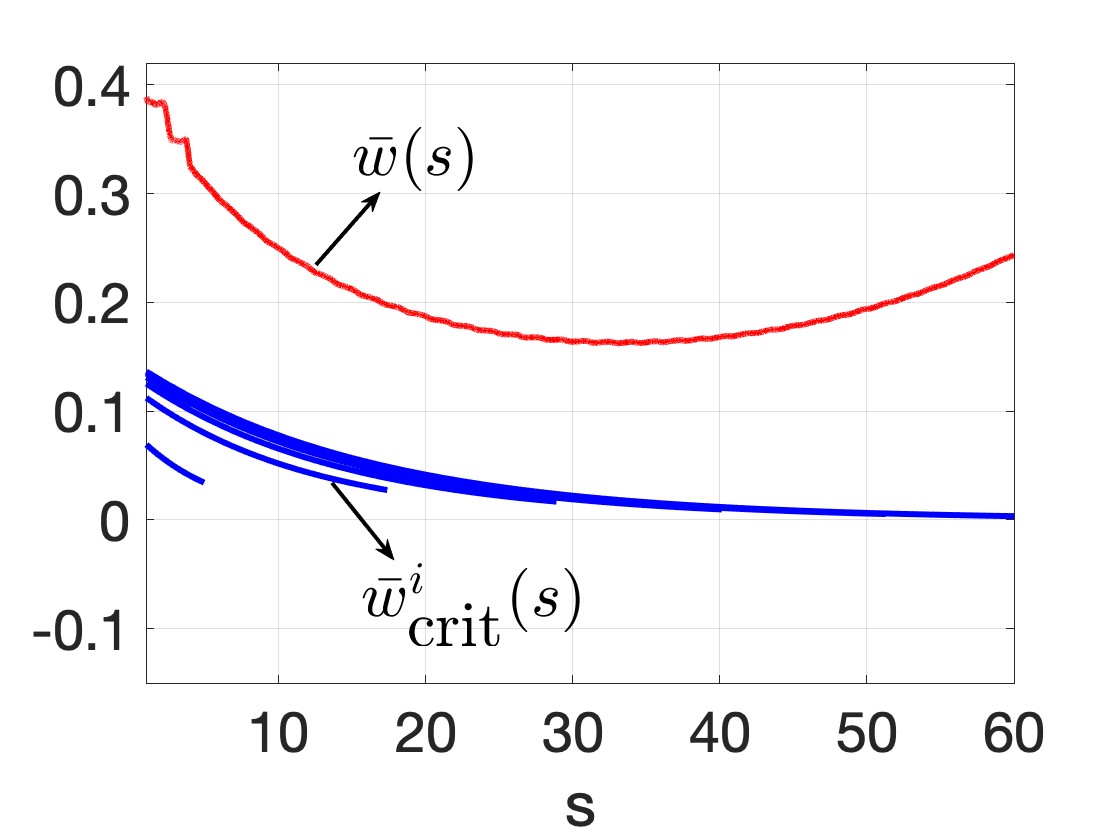
(a)

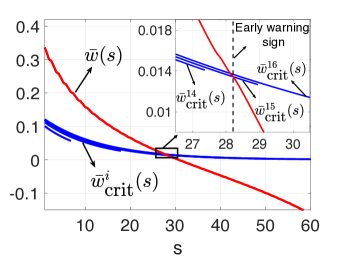
(b)

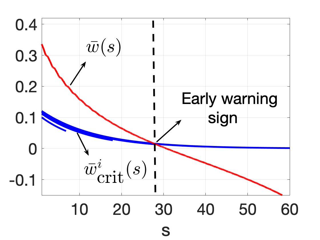
(c)

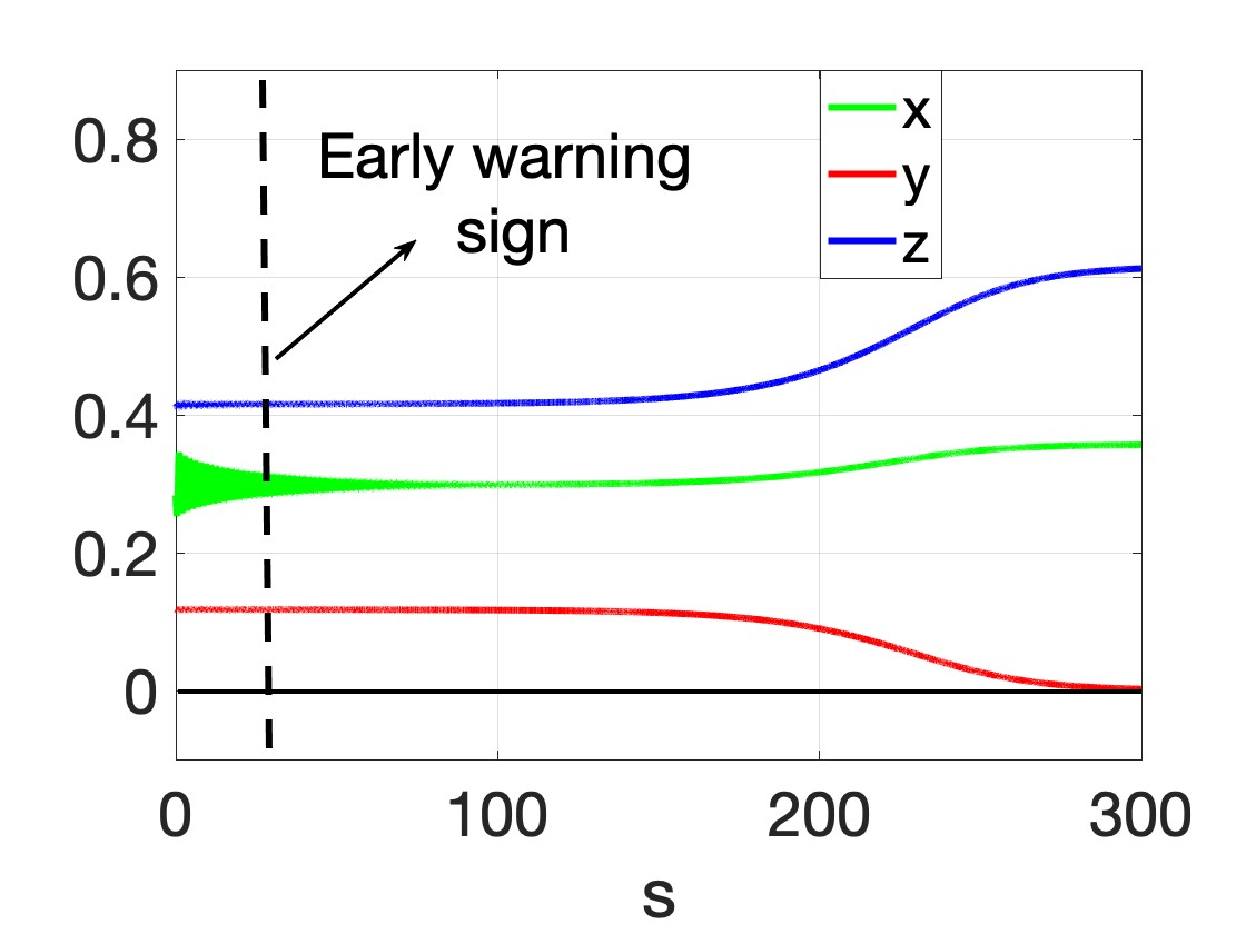
(d)

Figure 8. Detection of an early warning sign of species’ extinction in system (16) for initial conditions as in figure 1. (a) All species coexist as $\bar{w}(s)$ attains a global minimum. (b) One of the species will eventually extinct as predicted by the crossing of $\bar{w}$ with $\bar{w}^{15}_{\textrm{crit}}$. (c)-(d) Earliest warning sign of extinction of $y$ is detected at $s\approx 28.3$ when $\bar{w}(s)$ crosses $\bar{w}^{15}_{\textrm{crit}}(s)$.

6. Conclusion and outlook

Detection of early warning indicators of an impending population shift is challenging mainly due to the fact that the underlying mechanisms for regime shifts are not always known. The most common approach for calculating early warning signals is by analyzing bifurcation structures and time series data by examining trends of statistical summaries such as variance, autocorrelation, skewness and so forth [5, 6, 19]. In this paper we took a complementary approach for finding potential indicators of regime shifts by exploiting the geometry of the invariant manifolds in a general class of predator-prey models.

We focused on systems that exhibit bistability between a point attractor and a periodic attractor, where the attractors lie on the opposite sides of the stable eigenplane of a saddle-focus equilibrium, which lies in a vicinity of the singular Hopf point (FSN II bifurcation). The saddle-focus equilibrium has a one-dimensional unstable manifold with one of the branches of its unstable manifold tending to one of the attractors while the other tending to the other attractor. We took a systematic rigorous approach to unravel the dynamics near the saddle-focus equilibrium and predict asymptotic behaviors of solutions exhibiting nearly indistinguishable transient dynamics in a vicinity of the equilibrium. In view of the temporal dynamics, our analysis sheds light on the ability to not only distinguish between time series with contrasting long-term dynamics in spite of presenting similar trends at the onset (see figure 1), but also on the power to detect warning signals of catastrophic population collapses remarkably ahead of time as shown in figure 8. Since the dynamics studied in these models are associated with survivability and coexistence of species and thereby bear connections to the phenomena of permanence and persistence in ecological communities [9], we hope that our analysis can be useful in identifying an appropriate time for an intervention which might protect a vulnerable species from extinction.

The geometry of the class of equations studied in this paper can extend beyond predator-prey models. Systems with similar geometric configurations having multiple coexisting attractors whose basins of attraction are separated by the invariant manifolds of a saddle or a saddle-focus equilibrium can be analyzed using the techniques used in this paper. Some examples may include models arising from epidemiology and eco-epidemiology exhibiting bistability between endemic and disease-free equilibria, or between two endemic limit cycles or between a disease-free limit cycle and an endemic state (see [3] and the references therein). We hope that the approach used in this work is also useful from a broader dynamical systems point of view.

The method used to find an early warning signal can be possibly extended to mathematical models that have practical applications in environmental management. Viewing the dynamics through the lens of averaging, we note that our approach is analogous to the method of averaging [16, 30], a classical method used in analyzing weakly nonlinear oscillators and non-autonomous equations featuring two timescales that are widely separated. Thus our technique can be applied to a wide range of oscillatory dynamics characterized by two intrinsic timescales. Future directions on this work include expanding the analysis to parameter regimes where competitive exclusion of a species is preceded by long transients in form of mixed-mode oscillations [7, 13, 24] or amplitude-modulated oscillations past a torus bifurcation as seen in [25]. Other future work includes studying the effect of stochasticity on the system.

Appendix

The normal form variables $(u,v,w)$ in terms of $(x,y,z)$ are as follows:

$$\left\{\begin{array}[]{ll}u&=\frac{\bar{f_{1xx}}}{\omega}X-\delta(\bar{f_{1y}}B_{1}(A_{1},A_{2},X,Y,Z)+\bar{f_{1z}}B_{2}(A_{1},A_{2},X,Y,Z)\\ &+\frac{\delta}{3}C_{uv}\Big{[}\Big{(}\frac{\bar{f_{1xx}}}{\omega}X-\delta(\bar{f_{1y}}B_{1}(A_{1},A_{2},X,Y,Z)+\bar{f_{1z}}B_{2}((A_{1},A_{2},X,Y,Z))\Big{)}^{2}\\ &\Big{(}-1+\frac{\bar{f_{1xx}}}{2\omega^{2}}(\bar{f_{1y}}Y+\bar{f_{1}}_{z}Z)\Big{)}+\frac{\bar{f^{2}_{1xx}}}{\omega^{4}}(\bar{f_{1y}}Y+\bar{f_{1z}}Z)^{2}\Big{]},\\ v&=\frac{\bar{f_{1xx}}}{\omega^{2}}(\bar{f_{1y}}Y+\bar{f_{1z}}Z),\\ w&=-\frac{\bar{f_{1xx}}\bar{f_{1y}}}{\omega^{2}\bar{f_{1z}}}\Big{[}\Big{(}1+\frac{\bar{f_{2x}}\bar{f_{1}}_{y}}{\omega^{2}}\Big{)}Y+{\bar{f_{2x}}\bar{f_{1z}}}{\omega^{2}}Z+\frac{\delta}{\omega}\bar{f_{1}}_{xx}A_{1}X\Big{]},\end{array}\right.$$

where

$$X = \frac{x-x_{0}}{\sqrt{\zeta}},\ Y=\frac{y-y_{0}}{\zeta},\ Z=\frac{z-z_{0}}{\zeta},$$

$$A_{1} = \left(1+\frac{\bar{f_{2x}}\bar{f_{1y}}}{\omega^{2}}\right)(\bar{f_{2y}}\bar{f_{2x}}+\bar{f_{2z}}\bar{f_{3x}})+\frac{\bar{f_{2x}}\bar{f_{1z}}}{\omega^{2}}(\bar{f_{3y}}\bar{f_{2x}}+\bar{f_{3z}}\bar{f_{2x}}),$$

$$A_{2} = \frac{\bar{f_{3x}}\bar{f_{1y}}}{\omega^{2}}(\bar{f_{2y}}\bar{f_{2x}}+\bar{f_{2z}}\bar{f_{3x}})+\left(1+\frac{\bar{f_{3x}}\bar{f_{1z}}}{\omega^{2}}\right)(\bar{f_{3y}}\bar{f_{2x}}+\bar{f_{3z}}\bar{f_{2x}}),$$

$$C_{uv} = -\frac{1}{\omega^{2}}\Big{[}\bar{f_{1y}}(\bar{f_{2y}}\bar{f_{2x}}+\bar{f_{2z}}\bar{f_{3x}})+\bar{f_{1z}}(\bar{f_{3y}}\bar{f_{2x}}+\bar{f_{3z}}\bar{f_{2x}})\Big{]}$$

$$- \frac{1}{\bar{f_{1xx}}}\Big{[}\bar{f_{1xy}}\bar{f_{2x}}+\bar{f_{1xz}}\bar{f_{3x}}+\bar{f_{1y}}\bar{f_{2xx}}+\bar{f_{1z}}\bar{f_{3xz}}\Big{]},$$

$$B_{1} = \frac{1}{\omega^{2}}(\bar{f_{1y}}Y+\bar{f_{1z}}Z)(\bar{f_{2y}}\bar{f_{2x}}+\bar{f_{2z}}\bar{f_{3x}})+\frac{\bar{f_{1xx}}\bar{f_{2xx}}}{2\omega^{2}}+\frac{\bar{f_{2y}}\bar{f_{1xx}}}{\omega^{2}}\Big{[}\left(1+\frac{\bar{f_{2x}}\bar{f_{1y}}}{\omega^{2}}\right)Y$$

$$+ \frac{\bar{f_{2x}}\bar{f_{1z}}}{\omega^{2}}Z+\frac{\delta A_{1}X}{\omega}\Big{]}+\frac{\bar{f_{2z}}\bar{f_{1xx}}}{\omega^{2}}\Big{[}\frac{\bar{f_{3x}}\bar{f_{1y}}}{\omega^{2}}Y+\Big{(}1+\frac{\bar{f_{3x}}\bar{f_{1z}}}{\omega^{2}}\Big{)}Z+\frac{\delta A_{2}X}{\omega}\Big{]},$$

$$B_{2} = \frac{1}{\omega^{2}}(\bar{f_{1y}}Y+\bar{f_{1z}}Z)(\bar{f_{3y}}\bar{f_{2x}}+\bar{f_{3z}}\bar{f_{3x}})+\frac{\bar{f_{1xx}}\bar{f_{3xx}}}{2\omega^{2}}+\frac{\bar{f_{3y}}\bar{f_{1xx}}}{\omega^{2}}\Big{[}\left(1+\frac{\bar{f_{2x}}\bar{f_{1y}}}{\omega^{2}}\right)Y$$

$$+ \frac{\bar{f_{2x}}\bar{f_{1z}}}{\omega^{2}}Z+\frac{\delta A_{1}X}{\omega}\Big{]}+\frac{\bar{f_{3z}}\bar{f_{1xx}}}{\omega^{2}}\Big{[}\frac{\bar{f_{3x}}\bar{f_{1y}}}{\omega^{2}}Y+\Big{(}1+\frac{\bar{f_{3x}}\bar{f_{1z}}}{\omega^{2}}\Big{)}Z+\frac{\delta A_{2}X}{\omega}\Big{]}.$$

References

- [1] S. M. Baer and T. Erneux, Singular Hopf bifurcation to relaxation oscillations, SIAM Journal on Applied Mathematics, 46 (1986), pp. 721-739.
- [2] David K. A Barnes et al. Local Population Disappearance Follows (20 Yr after) Cycle Collapse in a Pivotal Ecological Species, Marine Ecology Progress Series, 226, (2002) pp. 311–313.
- [3] A.M. Bate, and F.M. Hilker, Complex Dynamics in an Eco-epidemiological Model, Bull. Math. Biol. 75, (2013) pp. 2059 - 2078.
- [4] B. Braaksma, Singular Hopf bifurcation in systems with fast and slow variables. J. Nonlinear Sci., 8(5), (1998) pp. 457–490.
- [5] C. Boettigera, N. Rossb, A. Hastings, Early warning signals: The charted and uncharted territories, Theor. Ecol. 6, (2013) pp. 255–264 .
- [6] C. Boettigera, A. Hastings, Quantifying limits to detection of early warning for critical transitions, J. Royal Soc. Interface. 7; 75, (2012) pp. 2527 - 2539.
- [7] B.M. Brns, M. Krupa, M. Wechselberger, Mixed Mode Oscillations Due to the Generalized Canard Phenomenon, Fields Institute Communications 49 (2006) pp. 39-63.
- [8] S. R. Carpenter, J. J. Cole, M. L. Pace, et al., Early warnings of regime shifts: A whole-ecosystem experiment, Science, 332, (2011) pp. 1079 - 1082.
- [9] S.R Cantrell and C. Cosner, Spatial Ecology via Reaction-Diffusion Equations, Wiley, 2004.
- [10] Glenn De’ath, K. E. Fabricius, H. Sweatman, and M. Puotinen, The 27–year decline of coral cover on the Great Barrier Reef and its causes, PNAS, 109 (44) (2012) pp. 17995 - 17999 .
- [11] B. Deng, Food chain chaos due to junction-fold point, Chaos 11 (2001) pp. 514-525.
- [12] B. Deng and G. Hines, Food chain chaos due to Shilnikov’s orbit, Chaos 12 (2002) pp. 533-538.
- [13] M. Desroches, J. Guckenheimer, B. Krauskopf, C. Kuehn, H.M. Osinga, M. Wechselberger, Mixed-Mode Oscillations with Multiple Time Scales, SIAM Review 54 (2012) pp. 211-288.
- [14] B. Ermentrout, Simulating, Analyzing, and Animating Dynamical Systems: A Guide to XPPAUT for Researchers and Students, SIAM, 2002.
- [15] J. Guckenheimer, Singular Hopf Bifurcation in Systems with Two Slow Variables, SIAM Journal of Applied Dynamical Systems 7 (2008) pp. 1355-1377.
- [16] J. Guckenheimer and P. Holmes, Nonlinear Oscillations, Dynamical Systems and Bifurcations of Vector Fields, Springer-Verlag, Berlin 1983.
- [17] A. Hastings, Transients: the key to long-term ecological understanding? Trends in Ecol. and Evol. 19 (2004).
- [18] A. Hastings, K. C. Abbott, K. Cuddington, T. Francis, G. Gellner, Y-C. Lai, A. Morozov, S. Petrovskii, K. Scranton, M.L. Zeeman, Transient phenomena in ecology, Science 07 (2018).
- [19] C. Kuehn, A mathematical framework for critical transitions: Bifurcations, fast–slow systems and stochastic dynamics, Physica D: Nonlinear Phenomena, 240 (2011) pp. 1020-1035.
- [20] Y.A.Kuznetsov, Elements of Applied BifurcationTheory, Springer, 1998.
- [21] A. Morozov, K. Abbott, K. Cuddington, T. Francis, G. Gellner, A. Hastings, Y.C. Lai, S. Petrovskii, K. Scranton, M.L. Zeeman, Long transients in ecology: theory and applications, Physics of Life Reviews, 32, (2020) pp. 1-40.
- [22] S. Muratori and S. Rinaldi, Remarks on competitive coexistence, SIAM J. Applied Math. 49 (1989) pp. 1462-1472.
- [23] S. Rinaldi and S. Muratori , Slow-fast limit cycles in predator-prey models, Ecol. Modelling 61 (1992) pp. 287-308.
- [24] S. Sadhu and S. Chakraborty Thakur, Uncertainty and Predictability in Population Dynamics of a Two-trophic Ecological Model: Mixed-mode Oscillations, Bistability and Sensitivity to Parameters, Ecol. Complexity 32 (2017) pp. 196-208.
- [25] S. Sadhu, Complex oscillatory patterns near singular Hopf bifurcation in a two time-scale ecosystem, DCDS, 26 (2021), pp. 5251-5279.
- [26] S. Sadhu, Analysis of the onset of a regime shift and detecting early warning signs of major population changes in a two-trophic three-species predator-prey model with long-term transients, J. Math. Biol. (accepted).
- [27] M. Scheffer and S. R. Carpenter, Catastrophic regime shifts in ecosystems: linking theory to observation, Trends in Ecol. and Evol. 18 (2003) pp. 648 -656.
- [28] M. Scheffer, Critical Transitions in Nature and Society, 16 Princeton University Press 2009.
- [29] M. Scheffer, D. Straile, E. H. van Nes, and H. Hosper. Climatic warming causes regime shifts in lake food webs, Limnol. Oceanogr. 46 (7), (2001) pp. 1780 - 1783.
- [30] F. Verhulst, Nonlinear Differential Equations and Dynamical Systems, Springer-Verlag: New York, Heidelberg, Berlin, 1993.