Dynamical quantum phase transitions in SYK Lindbladians

Abstract

We study the open quantum dynamics of the Sachdev-Ye-Kitaev (SYK) model described by the Lindblad master equation, where the SYK model is coupled to Markovian reservoirs with jump operators that are either linear or quadratic in the Majorana fermion operators. Of particular interest for us is the time evolution of the dissipative form factor, which quantifies the average overlap between the initial and time-evolved density matrices as an open quantum generalization of the Loschmidt echo. We find that the dissipative form factor exhibits dynamical quantum phase transitions. We analytically demonstrate a discontinuous dynamical phase transition in the limit of large number of fermion flavors, which is formally akin to the thermal phase transition in the two-coupled SYK model between the black-hole and wormhole phases. We also find continuous dynamical phase transitions that do not have counterparts in the two-coupled SYK model. While the phase transitions are sharp in the limit of large number of fermion flavors, their qualitative signatures are present even for the finite number of fermion flavors, as we show numerically.

I Introduction

The physics of open quantum systems has recently attracted growing interest. Since coupling to the external environment is unavoidable in realistic physical systems, an understanding of open quantum systems is important for quantum technology [1]. Notably, dissipation is not necessarily a nuisance that destroys quantum coherence and the concomitant quantum phenomena; rather, dissipation can even lead to new physical phenomena that have no analogs in closed quantum systems. For example, engineered dissipation can be utilized to prepare a desired quantum state [2, 3, 4]. Dissipation can also give rise to unique non-Hermitian topological phenomena [5]. Furthermore, open quantum systems exhibit phase transitions that cannot occur in closed quantum systems at thermal equilibrium [6, *Lee-Yang-52II, 8, 9, *Caldeira-Leggett-AP83, *Leggett-review, 12, 13, 14, 15, 16, 17]. Prime recent examples include the entanglement phase transitions induced by the competition between the unitary dynamics and the quantum measurements [18, 19, 20, *Li-19, 22, 23]. Despite these recent advances, the interplay of strong many-body interactions and dissipation, as well as the consequent phase transitions, has yet to be fully understood.

In the theory of phase transitions, it is important to develop a prototypical model that captures the universal behavior. Recently, open quantum generalizations of the Sachdev-Ye-Kitaev (SYK) model [24, 25] were proposed in Refs. [26, 27] as a prototype of open quantum many-body systems. In this model, dissipation is formulated by the Lindblad master equation [28, 29], which is different from the non-Hermitian SYK Hamiltonians [30, 31, 32, *Jian-21, 34]. The original SYK Hamiltonian is a fermionic model with fully-coupled random interactions and exhibits quantum chaotic behavior [24, 25, 35, 36, 37, 38, 39, 40, 41]. Similarly, the SYK Lindbladian is a prototype that exhibits the strongly-correlated chaotic behavior of open quantum systems [42, 43, 44, 45, 46, *Can-19JPhysA, 48, 49, 50, 51, 52, *Cornelius-22, 54]. As an advantage, the SYK Lindbladian is analytically tractable in the limit of the large number of fermion flavors even in the presence of dissipation. In Refs. [26, 27], the decay rate was analytically calculated in this limit, by which a transition between the underdamped and overdamped regimes was demonstrated. Still, the open quantum dynamics of the SYK Lindbladians remains mainly unexplored. As a prototype of open quantum many-body systems, the investigation into the SYK Lindbladians should deepen our general understanding of open quantum physics.

In this work, we find the dynamical quantum phase transitions in the SYK Lindbladians. We study the open quantum dynamics of the SYK Lindbladians and especially focus on the time evolution of the dissipative form factor. This quantifies the average overlap between the initial and time-evolved density matrices and serves as a partition function of the open quantum dynamics, similarly to the Loschmidt echo for the unitary dynamics of closed quantum systems. We find the singularities of the dissipative form factor as a function of time, which signal the dynamical quantum phase transitions similarly to the unitary counterparts [55, 56, 57, 58, 59, 60, 61, 62, 63, 64]. Notably, this quantum phase transition appears only in the dynamics in contrast with the conventional phase transitions for thermal equilibrium or ground states. In particular, we investigate the SYK Hamiltonian coupled to Markovian nonrandom linear dissipators and random quadratic dissipators. In the limit of the large number $N$ of fermions, we analytically obtain the dissipative form factor and demonstrate the discontinuous dynamical phase transition, which is formally akin to the thermal phase transition in the two-coupled SYK model between the black-hole and wormhole phases [65]. We also show the continuous dynamical transition that has no counterparts in the original two-coupled SYK model. Furthermore, we numerically show that signatures of the dynamical quantum phase transitions remain to appear even for finite $N$ although the singularities are not sharp.

The rest of this work is organized as follows. In Sec. II, we start by introducing the models, and review the quantity of our interest, the dissipative form factor. In Sec. III, we study the SYK Lindbladian with nonrandom linear jump operators. We discuss both numerics of the large $N$ saddle point equations and the analytical approach in the large $q$ limit. In Sec. IV, we study the SYK Lindbladian with random quadratic jump operators. We conclude in Sec. V.

II SYK Lindbladians and dissipative form factor

We consider Markovian dynamics of the density matrix $\rho(t)$ described by the Lindblad master equation [1]:

$$\frac{d}{dt}\rho(t) =\mathcal{L}(\rho(t))$$

$$\equiv-i[H,\rho(t)]$$

$$\qquad+\sum_{a}\left[L^{a}\rho(t)L^{a{\dagger}}-\frac{1}{2}\{L^{a{\dagger}}L^{a},\rho(t)\}\right],$$ (1)

where $H$ is the Hamiltonian, and $\{L^{a}\}$ is a set of jump operators that describe the dissipative process with the external environment. In our models, the Hamiltonian is given by the $q$-body SYK Hamiltonian

$$H^{\text{SYK}}=i^{q/2}\sum_{1\leq i_{1}<i_{2}<\cdots<i_{q}\leq N}J_{i_{1}i_{2}\cdots i_{q}}\psi^{i_{1}}\psi^{i_{2}}\cdots\psi^{i_{q}}.$$ (2)

Here, $\psi^{i=1,\dots,N}$ are Majorana fermion operators satisfying $\{\psi^{i},\psi^{j}\}=\delta_{ij}$. $J_{i_{1}\cdots i_{q}}$ are real independent Gaussian distributed random variables with zero mean and variance given by

$$\overline{(J_{i_{1}\cdots i_{q}})^{2}}=\sigma_{J}^{2}=\frac{J^{2}(q-1)!}{N^{q-1}}\quad\left(J\in\mathbb{R}^{+}\right),$$ (3)

where $\overline{\cdots}$ denotes the disorder average. We consider two choices of the jump operators: nonrandom linear and random quadratic. The nonrandom linear jump operators are

$$L^{i}=\sqrt{\mu}\psi^{i}\quad\left(i=1,\cdots,N,~{}\mu\in\mathbb{R}^{+}\right).$$ (4)

On the other hand, the random $p$-body jump operators are

$$L^{a}=\sum_{1\leq i_{1}<\cdots<i_{p}\leq N}K^{a}_{i_{1}\cdots i_{p}}\psi^{i_{1}}\cdots\psi^{i_{p}}\quad\left(a=1,2,\dots,M\right),$$ (5)

where $K^{a}_{i_{1}\cdots i_{p}}$ are complex Gaussian random variables with zero mean and variance given by

$$\overline{|K^{a}_{i_{1}\cdots i_{p}}|^{2}}=\sigma_{K}^{2}=\frac{K^{2}(p-1)!}{N^{p}}\quad\left(K\in\mathbb{R}^{+}\right).$$ (6)

In this work, we focus on $p=2$ for clarity.

Since the Lindbladian is a superoperator that acts on the density matrix, it is useful to introduce the operator-state map. Here, we vectorize the density matrix $\rho(t)$ and regard it as a state $\ket{\rho(t)}$ in the doubled Hilbert space $\mathcal{H}_{+}\otimes\mathcal{H}_{-}$. Correspondingly, we regard the Lindbladian as an operator acting on the doubled Hilbert space. For the SYK-type models relevant to this work, the Lindbladian acting on the doubled Hilbert space is given by

$$\mathcal{L} =-iH^{+}+i(-i)^{q}H^{-}$$

$$\qquad+\sum_{a}\left[(-i)^{p}L^{a}_{+}L^{a\dagger}_{-}-\frac{1}{2}L^{a\dagger}_{+}L^{a}_{+}-\frac{1}{2}L^{a}_{-}L^{a\dagger}_{-}\right],$$ (7)

where $H^{\pm}$ and $L_{\pm}^{a}$ act on $\mathcal{H}_{\pm}$, respectively. While the Hamiltonian part acts only on the individual bra or ket space, the dissipation term couples these two spaces.

A quantity of our central interest is the disorder-averaged trace of the exponential of the Lindbladian,

$$F(T_{L})=\overline{\mathrm{Tr}_{\mathcal{H}_{+}\otimes\mathcal{H}_{-}}\,(e^{T_{L}\mathcal{L}})},$$ (8)

which we call the dissipative form factor [46, *Can-19JPhysA, 52, *Cornelius-22]. The trace in Eq. (8) is taken over the doubled Hilbert space $\mathcal{H}_{+}\otimes\mathcal{H}_{-}$. As explained shortly, the dissipative form factor quantifies the average overlap between the initial and time-evolved density matrices and serves as the Loschmidt echo of open quantum systems. In the following, we obtain the dissipative form factor of the SYK Lindbladians, using both the analytical calculations for large $N$ and the numerical calculations for finite $N$, and demonstrate its singularities in the open quantum dynamics—dynamical quantum phase transitions. More specifically, we analyze (a dissipative analog of) the rate function of the dissipative form factor:

$$i\mathcal{S}(T_{L})\equiv\lim_{N\rightarrow\infty}\frac{\log F(T_{L})}{N}.$$ (9)

Although the spectrum of the Lindbladian is complex in general, the rate function is always real since the spectrum is symmetric about the real axis. We also note that the dissipative form factor does not depend on initial conditions but is determined solely by the Lindbladian. At $T_{L}=0$, we always have $F(T_{L}=0)=2^{N}$ and hence $i\mathcal{S}(T_{L}=0)=\log 2$.

Several motivating comments are in order. First, in the absence of dissipation, the dissipative form factor in Eq. (8) coincides with the spectral form factor of Hermitian Hamiltonians. In fact, we have

$$\mathrm{Tr}_{\mathcal{H}_{+}\otimes\mathcal{H}_{-}}\,(e^{T_{L}\mathcal{L}})$$

$$\quad=\mathrm{Tr}_{\mathcal{H}_{+}}\big{(}e^{-iT_{L}H^{+}}\big{)}\,\mathrm{Tr}_{\mathcal{H}_{-}}\big{(}e^{+iT_{L}(-i)^{q}H^{-}}\big{)}$$

$$\quad=\left|\mathrm{Tr}_{\mathcal{H}}\left(e^{-iT_{L}H}\right)\right|^{2},$$ (10)

where in the last line we take $q\equiv 0$ (mod $4$) for simplicity. Since the spectral form factor captures the quantum chaos of the SYK-type Hamiltonians [38], we expect that the dissipative form factor in Eq. (8) also captures the quantum chaos of the SYK Lindbladians. Accordingly, in the absence of the dissipation, the definition of the rate function in Eq. (9) coincides with its unitary analog. In the unitary case, non-analytical behavior in the rate function as a function of time was proposed as a diagnostic of the dynamical quantum phase transitions [55, 56, 57, 58, 59, 60, 61, 62, 63, 64]. Here, we extend this idea to the non-unitary case. We also note that there is another related quantity, dissipative spectral form factor, introduced in Ref. [54]. The dissipative spectral form factor captures the complex-spectral correlations of non-Hermitian operators. By contrast, the dissipative form factor in Eq. (8) is more directly relevant to the open quantum dynamics since it gives the Loschmidt echo and the decoherence rate, as explained below. These two quantities are thus complementary to understand the quantum chaos of open systems. While we focus on the dissipative form factor in this work, it should be worthwhile to study the dissipative spectral form factor of the SYK Lindbladians as future work.

Second, the dissipative form factor in Eq. (8) is related to the Loschmidt echo, the overlap between the initial and time-evolved states,

$$\mathrm{Tr}_{\mathcal{H}}\,\left[\rho(0)\rho(T_{L})\right].$$ (11)

With the operator-state map, the Loschmidt echo is written as the overlap between the two pure states in the doubled Hilbert space,

$$\langle\rho(0)|\rho(T_{L})\rangle=\langle\rho(0)|e^{T_{L}\mathcal{L}}|\rho(0)\rangle,$$ (12)

where $|\rho(0)\rangle\in\mathcal{H}_{+}\otimes\mathcal{H}_{-}$ is the state in the doubled Hilbert space $\mathcal{H}_{+}\otimes\mathcal{H}_{-}$ mapped from the density matrix $\rho(0)$. To make a contact with the dissipative form factor, one needs to average over the initial states $|\rho(0)\rangle$. For example, if we consider a set of states generated from a reference state $\rho_{0}$ by a unitary rotation,

$$\rho_{U}=U\rho_{0}U^{{\dagger}},$$ (13)

and average over the Haar random measure, we obtain

$$\int dU\,\langle\rho_{U}|e^{T_{L}\mathcal{L}}|\rho_{U}\rangle$$

$$\qquad=\frac{\mathrm{Tr}\,(\rho^{2}_{0})-1/L}{L^{2}-1}\,\mathrm{Tr}\,(e^{T_{L}\mathcal{L}})+\frac{L-\mathrm{Tr}\,(\rho^{2}_{0})}{L^{2}-1},$$ (14)

where $L$ is the dimensions of the Hilbert space ($L=2^{N/2}$ for the SYK-type models). Thus, the Loschmidt echo of open quantum systems is given by the dissipative form factor in Eq. (8). Here, if we choose $\rho_{0}$ to be the fully mixed state $\rho_{0}=1/L$, the first term in the right hand side of Eq. (II) vanishes. This is consistent with the fact that the fully mixed state cannot be decohered any longer. We have to avoid such a special reference state to connect the dissipative form factor with the average Loschmidt echo.

Finally, the dissipative form factor in Eq. (8) is also related to the decoherence rate [43] averaged over initial states. The decoherence rate $D$ quantifies the early-time decay of purity, defined by

$$D =\left.-\frac{2\,\mathrm{Tr}\,\left[\rho(0)(d\rho(t)/dt)\right]}{\mathrm{Tr}\,[\rho(0)^{2}]}\right|_{t=0}.$$ (15)

As before we average over initial states $\rho_{U}$, leading to

$$D_{{\rm av}} =-\frac{2}{\mathrm{Tr}\,[\rho^{2}_{0}]}\left.\frac{d}{dt}\int dU\,\mathrm{Tr}\,\left[\rho_{U}(0)\rho_{U}(t)\right]\right|_{t=0}.$$ (16)

Thus, the average decoherence rate $D_{\rm av}$ is given by the time derivative of the dissipative form factor at $t=0$. In particular, from Eq. (II), $D_{{\rm av}}$ is expressed as

$$D_{{\rm av}} =-\frac{2}{\mathrm{Tr}\,[\rho^{2}_{0}]}\frac{\mathrm{Tr}\,(\rho^{2}_{0})-1/L}{L^{2}-1}\,\mathrm{Tr}\,(\mathcal{L}).$$ (17)

III Nonrandom linear jump operators

Table 1: Analogy between the two-coupled SYK model [65] and the SYK Lindbladian with the nonrandom linear jump operators for the small coupling $\mu$. The wormhole in the coupled SYK model corresponds to the thermofield double (TFD) state at a certain temperature determined by $\mu$. Similarly, for the Lindbladian SYK model, the late time solution corresponds to the infinite temperature TFD state, which is the stationary state of the Lindbladian.

Two-coupled SYK model	SYK Lindbladian with the nonrandom linear dissipators
Left/Right system	Bra (+)/Ket ($-$) contour
$H=H^{L}_{\mathrm{SYK}}+(-1)^{\frac{q}{2}}H^{R}_{\mathrm{SYK}}+i\mu\sum_{i}\psi_{L}^{i}\psi_{R}^{i}$	$\mathcal{L}=-iH_{\mathrm{SYK}}^{+}+i(-1)^{\frac{q}{2}}H_{\mathrm{SYK}}^{-}-i\mu\sum_{i}\psi_{+}^{i}\psi_{-}^{i}-\mu\frac{N}{2}\mathbb{I}$
Inverse temperature $\beta$	Time $T_{L}$
Partition function $\mathrm{Tr}\,(e^{-\beta H})$	Dissipative form factor $\mathrm{Tr}\,(e^{T_{L}\mathcal{L}})$
Energy $E=\expectationvalue{H}$	Lindbladian $\expectationvalue{\mathcal{L}}$ (average decoherence rate)
Specific heat $C=\expectationvalue{H^{2}}-\expectationvalue{H}^{2}$
Energy gap	Decay rate
Black hole	Early time complex solution
Wormhole (TFD)	Late time real solution (infinite temperature TFD)
Hawking-Page transition	Late time first-order transition (real-complex spectral transition?)
N/A	Early time second-order order transition
Real time physics (e.g. chaos exponents)	?

We consider the SYK model with the nonrandom linear jump operators in Eq. (4). We notice that this open quantum model resembles the two-coupled SYK model (Maldacena-Qi model) [65], although the SYK Lindbladian is non-Hermitian while the two-coupled SYK model is Hermitian. As we will show below, there are many analogies between these models. In Table 1, we summarize the similarities and differences between the two-coupled SYK model and the SYK Lindbladian with the linear jump operators. In fact, one obtains the SYK Lindbladian from the two-coupled SYK model by an analytical continuation of the coupling $\mu$ from a real to pure imaginary value. In the Hermitian two-coupled SYK model, the finite temperature partition function was studied and the Hawking-Page transition (the thermal phase transition between the black hole and wormhole phases) was identified [65]. On the other hand, we are here interested in the dissipative form factor in Eq. (8), where $T_{L}$ plays the role of the real (rather than imaginary) time.

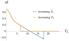
(a) $\mu=0.1$, large $N$

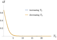
(b) $\mu=0.5$, large $N$

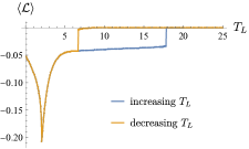
(c) $\mu=0.1$, large $N$

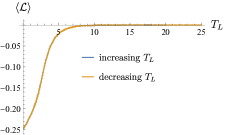
(d) $\mu=0.5$, large $N$

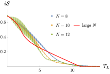
(e) $\mu=0.1$, finite $N$

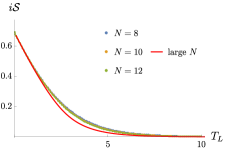
(f) $\mu=0.5$, finite $N$

Figure 1: Time evolution of the rate function (Loschmidt amplitude) $i\mathcal{S}$ of the SYK Lindbladian ($J=1$) with the nonrandom linear dissipators for (a) weak dissipation $\mu=0.1$ and (b) strong dissipation $\mu=0.5$. We obtain the rate function by solving the large $N$ saddle point equation numerically by increasing (blue curve) and decreasing (orange curve) $T_{L}$. (a) In the weak-dissipation regime, the two saddle point solutions are different from each other for $7\lessapprox T_{L}\lessapprox 18$, which signals a discontinuous phase transition around $T_{L}\approx 11$. The second-order derivative of the rate function $i\mathcal{S}$ is discontinuous around $T_{L}\approx 2$, which corresponds to a continuous phase transition. (b) In the strong-dissipation regime, no dynamical quantum phase transitions occur. In (c) and (d), the derivatives of the rate functions are shown, which are equivalent to the expectation values $\langle\mathcal{L}\rangle$ of the Lindbladians [see Eq. (25)]. In (e) and (f), comparisons with finite $N$ results from exact diagonalization of the Lindbladian are presented for $N=8,10,12$, where the error bars show sample-to-sample fluctuations.

III.1 Large $N$ analysis

The steady-state Green’s functions of the SYK Lindbladian were studied in Ref. [27] on the basis of the large $N$ techniques. Here, we study the dissipative form factor in a similar fashion, by imposing the anti-periodic boundary conditions for the fermion fields. Here, the anti-periodic boundary conditions arise naturally from the coherent state path integral representation of $\mathrm{Tr}\,e^{T_{L}{\cal L}}$, in much the same way as the regular Euclidean (imaginary time) path integral. Under these boundary conditions, the dissipative form factor is given by the Schwinger-Keldysh path integral,

$$F(T_{L})=\int\mathcal{D}\psi_{+}\mathcal{D}\psi_{-}e^{iS[\psi_{+},\psi_{-}]},$$ (18)

where the action $iS[\psi_{+},\psi_{-}]$ is

$$iS[\psi_{+},\psi_{-}] =\int_{0}^{T_{L}}dt\Big{[}-\frac{1}{2}\sum_{i}\psi^{i}_{+}\partial_{t}\psi^{i}_{+}-\frac{1}{2}\sum_{i}\psi^{i}_{-}\partial_{t}\psi^{i}_{-}+\mathcal{L}(t)\Big{]}$$

$$=\int_{0}^{T_{L}}dt\Bigg{[}-\frac{1}{2}\sum_{i}\psi^{i}_{+}\partial_{t}\psi^{i}_{+}-\frac{1}{2}\sum_{i}\psi^{i}_{-}\partial_{t}\psi^{i}_{-}-i^{\frac{q}{2}+1}\sum_{i_{1}<\cdots<i_{q}}J_{i_{1}\cdots i_{q}}\psi_{+}^{i_{1}}\cdots\psi_{+}^{i_{q}}$$

$$\qquad\qquad-(-i)^{\frac{q}{2}+1}\sum_{i_{1}<\cdots<i_{q}}J_{i_{1}\cdots i_{q}}\psi_{-}^{i_{1}}\cdots\psi_{-}^{i_{q}}-i\mu\sum_{i}\psi_{+}^{i}(t)\psi_{-}^{i}(t)-\mu\frac{N}{2}\int dt\Bigg{]}.$$ (19)

In terms of the collective variables $(G,\Sigma)$, we rewrite the dissipative form factor as

$$F(T_{L})=\int\mathcal{D}G\mathcal{D}\Sigma\ e^{iS[G,\Sigma]},$$ (20)

where the action $S[G,\Sigma]$ is

$$S[G,\Sigma] =-\frac{iN}{2}\Tr\log[-i(G_{0}^{-1}-\Sigma)]+\frac{i^{q+1}J^{2}N}{2q}\int_{0}^{T_{L}}dt_{1}dt_{2}\sum_{\alpha\beta}s_{\alpha\beta}G_{\alpha\beta}(t_{1},t_{2})^{q}$$

$$\qquad+\frac{iN}{2}\int_{0}^{T_{L}}dt_{1}dt_{2}\sum_{\alpha\beta}\Sigma_{\alpha\beta}(t_{1},t_{2})G_{\alpha\beta}(t_{1},t_{2})-i\frac{\mu N}{2}\int_{0}^{T_{L}}dt[G_{+-}(t,t)-G_{-+}(t,t)]+i\frac{\mu N}{2}\int dt.$$ (21)

Here, $\alpha,\beta=+,-$ and $s_{\alpha\beta}$ is

$$s_{++}=s_{--}=1,\qquad s_{+-}=s_{-+}=-(-1)^{\frac{q}{2}}.$$ (22)

For large $N$, the path integral in Eq. (20) is dominated by the saddle point. The large $N$ saddle point equation is

$$i\partial_{t_{1}}G_{\alpha\beta}(t_{1},t_{2})-\int dt_{3}\sum_{\gamma=+,-}\Sigma_{\alpha\gamma}(t_{1},t_{3})G_{\gamma\beta}(t_{3},t_{2})=\delta_{\alpha\beta}\delta(t_{1}-t_{2}),$$

$$\Sigma_{\alpha\beta}(t_{1},t_{2})=-i^{q}J^{2}s_{\alpha\beta}G_{\alpha\beta}(t_{1},t_{2})^{q-1}+\mu\epsilon_{\alpha\beta}\delta(t_{1}-t_{2}).$$ (23)

The dissipative form factor is then calculated from the on-shell action:

$$F(T_{L})\approx e^{iS[G_{*},\Sigma_{*}]},$$ (24)

where $G_{*}$ and $\Sigma_{*}$ are solutions to Eq. (23).

We compute the expectation value of the Lindbladian from the derivative of the dissipative form factor,

$$\frac{\partial}{\partial T_{L}}\log F(T_{L})=\langle\mathcal{L}\rangle\equiv\frac{\overline{\Tr(\mathcal{L}e^{T_{L}\mathcal{L}})}}{\overline{\Tr(e^{T_{L}\mathcal{L}})}}.$$ (25)

In our problem, the dissipative form factor is expected to be self-averaging. For $T_{L}=0$, this quantity essentially gives the average decoherence rate in Eq. (17). Using the canonical commutation relation, we derive the relation between $\langle\mathcal{L}\rangle$ and the correlation function as follows:

$$\frac{\langle\mathcal{L}\rangle}{N} =-\frac{i}{q}\lim_{t\to 0^{+}}\partial_{t}G_{++}(t)-\frac{i}{q}\lim_{t\to 0^{+}}\partial_{t}G_{--}(t)+\mu\Big{(}1-\frac{2}{q}\Big{)}G_{+-}(0)-\frac{\mu}{2}.$$ (26)

Here, the two-point correlation functions depend only on the time difference because of the cyclicity of the trace and concomitant time-translation invariance. Employing the Kadanoff-Baym equation, we find another representation of $\langle\mathcal{L}\rangle$ as

$$\frac{\langle\mathcal{L}\rangle}{N}=i\frac{i^{q+1}J^{2}}{q}\int_{0}^{T_{L}}\sum_{\alpha,\beta}s_{\alpha\beta}G_{\alpha\beta}(t)^{q}dt+\mu G_{+-}(0)-\frac{\mu}{2}.$$ (27)

We rewrite the latter representation as

$$T_{L}\frac{\partial{\cal S}}{\partial T_{L}}=J\frac{\partial{\cal S}}{\partial J}+\mu\frac{\partial{\cal S}}{\partial\mu},$$ (28)

which is considered to be an Euler relation for the dissipative form factor.

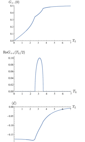
Figure 2: Second-order dynamical quantum phase transitions in the SYK Lindbladian with the nonrandom linear dissipators ($q=4$, $J=1$, $\mu=0.35$). The Green’s functions $G_{+-}(0)$ and $\mathrm{Re}\,G_{++}(T_{L}/2)$ exhibit cusps at $T_{L}\approx 2.6$ and $T_{L}\approx 3.6$, while the singularities in $\langle{\cal L}\rangle$ are unclear.

As shown in Fig. 1, we calculate the rate function $i\mathcal{S}$ as a function of time $T_{L}$. In these calculations, we obtain the two different saddle point solutions, depending on whether we increase or decrease $T_{\rm L}$. For given $T_{L}$, we need to take the dominant one (i.e., maximizing $i\mathcal{S}$). For the strong dissipation $\mu=0.5$, the two saddle point solutions are identical [Fig. 1 (b)]. On the other hand, for the smaller dissipation $\mu=0.1$, the two solutions disagree for the intermediate times $7\lessapprox T_{L}\lessapprox 18$, and the rate function $i\mathcal{S}$ exhibits more complex behaviors as a function of $T_{L}$. At early time, the Green’s functions of the dominant saddle point closely resemble the dissipation-free unitary solution. This saddle corresponds to the black hole in the two-coupled SYK model. Around $T_{L}\approx 2$, the second-order derivative of the rate function (Loschmidt amplitude) exhibits a discontinuous change, which signals the continuous dynamical quantum phase transition. In addition, around $T_{L}\approx 11$, a discontinuous phase transition occurs when the other solution arising from dissipation becomes dominant and remains so for all subsequent $T_{L}$. This saddle corresponds to the wormhole in the two-coupled SYK model. For $T_{L}\to\infty$, this dissipative solution indeed relaxes to the steady-state Green’s function obtained in Ref. [27], and corresponds to the infinite temperature thermofield double state. It is worth recalling that, in the finite $N$ spectral analysis in Ref. [27], all the eigenvalues approach the real axis as we increase the dissipation strength $\mu$, similar to a real-complex spectral transition in non-Hermitian systems [12, 44].

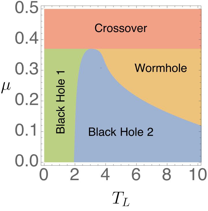
Figure 3: Dynamical phase diagram of the SYK Lindbladian with the nonrandom linear jump operators in terms of time $T_{L}$ and dissipation strength $\mu$ ($q=4$, $J=1$). The three phases are defined by $G_{++}(t)\in\mathbb{R}$, $G_{+-}(t)\not\equiv 0$ (green region, Black Hole 1), $G_{++}(t)\in\mathbb{C}$, $G_{+-}(t)\not\equiv 0$ (blue region, Black Hole 2), and $G_{++}(t)\in\mathbb{R}$, $G_{+-}(t)\not\equiv 0$ (orange region, Wormhole). For the strong dissipation $\mu\gtrapprox 0.37$, sharp quantum phase transitions are replaced by crossover, and there are no clear distinction between Black Hole 1 phase and Wormhole phase through the order parameters $G_{++}(t)$ and $G_{+-}(t)$.

As we change the dissipation strength $\mu$, the presence or absence of these transitions, and also their characters, change. For small enough $\mu$, we have the first- and second-order phase transitions as described above. As we increase $\mu$, for the intermediate values of $\mu$, the first-order transition is transmuted into second-order, and we have two second-order transitions. In Fig. 2, we demonstrate the existence of the two second-order phase transitions by plotting the Green’s functions at particular times, $G_{+-}$ at $t=0$ and the real part of $G_{++}$ at $t=T_{L}/2$, in addition to the time derivative of the rate function [i.e., expectation value $\langle\mathcal{L}\rangle$ of the Lindbladian; see Eq. (25)]. While the singularities in $\langle{\cal L}\rangle$ are somewhat difficult to see in these plots, the Green’s functions exhibit clearer cusp behaviors. Finally, for large enough $\mu$, the two second-order transitions merge and we do not have any transitions. We provide the phase diagram in Fig. 3. In the next subsection, we confirm these behaviors analytically in the large $q$ limit (see, e.g., Fig. 6).

Furthermore, we obtain the rate function also for finite $N$ and compare the finite $N$ numerical results with the large $N$ analytical results [Fig. 1 (c, d)]. While the phase transitions sharply occur only for large $N$, the characteristic behaviors of the phase transitions have an inkling already in the finite $N$ numerics. In fact, the rate functions for finite $N$ diminish to nearly zero around the expected discontinuous phase transition point $T_{L}\approx 11$. In addition, around $T_{L}\approx 2$, the sample-to-sample fluctuations of the rate function are enhanced, which is consistent with the continuous phase transition for large $N$.

III.2 Large $q$ analysis

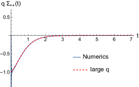
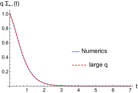
Figure 4: Comparison between the analytically obtained real solution for large $q$ (red dashed curve) and the numerically obtained solution for $q=96$ (blue solid curve). The other parameters are chosen to be $\mathcal{J}=1$, $\hat{\mu}=0.5$, and $T_{L}=700$. The vertical axis is $q\Sigma_{\alpha\beta}\simeq\mathcal{J}^{2}e^{g_{\alpha\beta}}$.

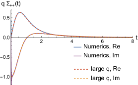
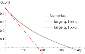
Figure 5: Comparison between the large $q$ complex solution and the numerical solutions ($q=96$, $\mathcal{J}=1$, $\hat{\mu}=0.5$, $T_{L}=700$). The vertical axis is $q\Sigma_{++}\simeq\mathcal{J}^{2}e^{g_{++}}$ for the left panel and $G_{+-}$ for the right panel.

The large $N$ saddle point equations are analytically tractable in the large $q$ limit [36]. Reference [27] utilized the large $q$ limit of the SYK Lindbladian with the nonrandom linear jump operators and calculated the stationary properties. Here, we apply the large $q$ technique to calculate the dissipative form factor. The large $q$ analysis has to be done separately for different time scales. In the following, we mainly focus on the regime where $T_{L}$ is of order $O(q\log q)$, where, as we show below, both first- and second-order transitions mentioned above occur.

We start by expanding the correlation functions for small $t$ (i.e., $t\ll q$) as

$$G_{++}(t_{1},t_{2}) =-\frac{i}{2}\text{sgn}(t_{1}-t_{2})\Big{(}1+\frac{1}{q}g_{++}(t_{1},t_{2})+\cdots\Big{)},$$

$$G_{+-}(t_{1},t_{2}) =+\frac{1}{2}\Big{(}1+\frac{1}{q}g_{+-}(t_{1},t_{2})+\cdots\Big{)},$$

$$G_{-+}(t_{1},t_{2}) =-\frac{1}{2}\Big{(}1+\frac{1}{q}g_{-+}(t_{1},t_{2})+\cdots\Big{)},$$

$$G_{--}(t_{1},t_{2}) =-\frac{i}{2}\text{sgn}(t_{1}-t_{2})\Big{(}1+\frac{1}{q}g_{--}(t_{1},t_{2})+\cdots\Big{)}.$$ (29)

In the large $q$ limit, the Kadanoff-Baym equation reduces to the Liouville equation,

$$\partial_{t_{1}}\partial_{t_{2}}g_{++}(t_{1},t_{2}) =-2\mathcal{J}^{2}e^{g_{++}(t_{1},t_{2})},$$

$$\partial_{t_{1}}\partial_{t_{2}}g_{+-}(t_{1},t_{2}) =-2\mathcal{J}^{2}e^{g_{+-}(t_{1},t_{2})}-2\hat{\mu}\delta(t_{1}-t_{2}),$$ (30)

where we define $\mathcal{J}$ and $\hat{\mu}$ by

$$J^{2}\equiv\frac{2^{q-1}\mathcal{J}^{2}}{q},\quad\mu\equiv\frac{\hat{\mu}}{q}.$$ (31)

The Liouville equation admits multiple solutions, as in the case of finite $q$. In the following, we study two types of solutions with real $g_{++}$ and complex $g_{++}$, which we call real and complex solutions, respectively.

Real solutions.

We solve the Liouville equation for stationary states as

$$e^{g_{++}(t)} =\frac{\alpha^{2}}{\mathcal{J}^{2}\cosh^{2}(\alpha|t|+\gamma)},$$

$$e^{g_{+-}(t)} =\frac{\tilde{\alpha}^{2}}{\mathcal{J}^{2}\cosh^{2}(\tilde{\alpha}|t|+\tilde{\gamma})}.$$ (32)

The boundary conditions $G_{++}(0,0)=G_{--}(0,0)=-i/2$ and $\lim_{t_{2}\to t_{1}}\partial_{t_{1}}g_{+-}(t_{1},t_{2})=-\hat{\mu}$ give the relations

$$\alpha=\mathcal{J}\cosh\gamma,\quad 2\tilde{\alpha}\tanh\tilde{\gamma}=\hat{\mu}.$$ (33)

For long time $t\gg q$, $g_{\alpha\beta}$ becomes of order $q$, and the expansion in Eq. (29) breaks down. Hence, for such a long time, we use a different approximation [65, 68]. Because $\Sigma_{\alpha\beta}(t)$ varies much more rapidly than $G_{\alpha\beta}$ in the large $q$ limit, we can approximate $\Sigma_{\alpha\beta}(t)$ by delta functions or its derivative. From the symmetry of the function, we can approximate

$$\Sigma_{++}(t)=\Sigma_{--}(t)\simeq\rho\delta^{\prime}(t),$$

$$\Sigma_{+-}(t)=-\Sigma_{-+}(t)\simeq\nu\delta(t),$$ (34)

where $\rho$ and $\nu$ are of order $q$. However, the convolution with $\Sigma_{++}(t)$ and $\Sigma_{--}(t)$ leads to the derivative of $G_{\alpha\beta}$, which already exists in the Kadanoff-Baym equation and gives the subleading contribution in the large $q$ expansion. Therefore, we can ignore them, and the equation becomes

$$i\partial_{t}G_{++}(t)-\nu G_{-+}(t)=0,$$

$$i\partial_{t}G_{+-}(t)-\nu G_{--}(t)=0,$$

$$i\partial_{t}G_{-+}(t)+\nu G_{++}(t)=0,$$

$$i\partial_{t}G_{--}(t)+\nu G_{+-}(t)=0,$$ (35)

where $\nu$ is related to the parameter of the $t\ll q$ solution by

$$\nu=\int_{-\infty}^{\infty}\Sigma_{+-}(t)dt=\frac{\mu}{\tanh\tilde{\gamma}}.$$ (36)

Here, the delta function $\mu\delta(t)$ is included as the boundary conditions of $g_{+-}(t)$ at the origin by $\partial_{t}g_{+-}(0)=-\hat{\mu}$. We rewrite the above condition as

$$T_{L}\mu=\tanh\tilde{\gamma}\log\frac{q}{\sigma},$$ (37)

where we introduce an order $O(1)$ parameter

$$\sigma=qe^{-\nu T_{L}}.$$ (38)

The solution of Eq. (35) with the correct boundary conditions is then

$$G_{++}(t) =-iA\cosh\nu\Big{(}\frac{T_{L}}{2}-t\Big{)},$$

$$G_{+-}(t) =A\sinh\nu\Big{(}\frac{T_{L}}{2}-t\Big{)},$$ (39)

with $G_{-+}(t)=-G_{+-}(t)$, $iG_{--}(t)=(iG_{++}(t))^{*}$, $G_{++}(T_{L}-t)=G_{++}(t)$, and $G_{+-}(T_{L}-t)=-G_{+-}(t)$.

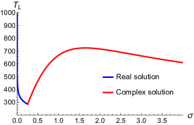
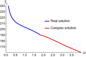
Figure 6: $T_{L}$ as a function of $\sigma$ in the large $q$ solutions for $q=96$. (Left) For the weak dissipation $\hat{\mu}=0.5$, $T_{L}$ is not a monotonic function of $\sigma$, and for fixed $T_{L}$, there are one real and two complex solutions in the intermediate regime. (Right) For the strong dissipation $\hat{\mu}=1.9$, $T_{L}$ is a monotonic function of $\sigma$, but the derivative is not continuous when the real and complex saddles meet.

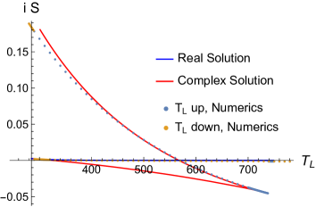
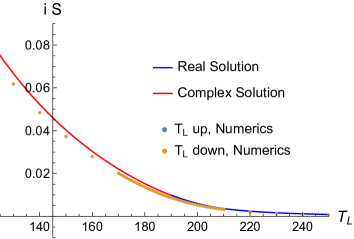
Figure 7: Rate function $i\mathcal{S}$ in the large $q$ limit with $q=96$ and $\mathcal{J}=1$ for (Left) $\hat{\mu}=0.5$ and (Right)  $\hat{\mu}=1.9$. For comparison, we also plot the numerical solutions of the saddle point equations (blue and orange dots).

The matching of the $t\ll q$ and $t\gg q$ solutions at the overlapping region fixes the parameters as

$$A=e^{-\frac{\nu}{2}T_{L}},\quad\alpha=\tilde{\alpha}=\frac{q\nu}{2},\quad\tilde{\gamma}-\gamma=\sigma.$$ (40)

The conditions in Eqs. (33), (36), and (40) determine the free parameters $\alpha,\tilde{\alpha},\gamma,\tilde{\gamma},A$, and $\nu$ as functions of $\hat{\mu}$ and $T_{L}$. Note $\gamma=0$ for $\hat{\mu}=2\mathcal{J}\tanh\sigma$. For $\hat{\mu}>2\mathcal{J}\tanh\sigma$, there is no real positive solution for $\gamma$. We compare the large $q$ solution with the numerical solutions for $q=96$ in Fig. 4, which are consistent with each other.

From Eq. (27), we obtain the expectation value of the Lindbladian as

$$\frac{\expectationvalue{\mathcal{L}}}{N}=\frac{\hat{\mu}}{q^{2}}\bigg{(}\frac{\tanh\gamma}{\tanh\tilde{\gamma}}-1+\log\frac{\cosh\gamma}{\cosh\tilde{\gamma}}\bigg{)}.$$ (41)

Accordingly, the rate function of the dissipative form factor is

$$i\mathcal{S}(\sigma,\gamma)=\frac{T_{L}\hat{\mu}}{q^{2}}\bigg{(}-1+\frac{\tanh\gamma}{\tanh\tilde{\gamma}}+\log\frac{\cosh\gamma}{\cosh\tilde{\gamma}}+\frac{\sigma}{\tanh\tilde{\gamma}}\bigg{)}+\frac{\sigma}{q}.$$ (42)

Complex solutions.

In the real solution in Eq. (III.2), the parameters $\alpha$, $\tilde{\alpha}$, $\gamma$, and $\tilde{\gamma}$ are real. We now relax this condition and look for the complex solution. In particular, we look for the solution of the form

$$e^{g_{++}(t)} =\frac{\alpha}{\mathcal{J}^{2}\cosh^{2}(\alpha|t|+i\gamma_{i})},$$

$$e^{g_{+-}(t)} =\frac{\tilde{\alpha}^{2}}{\mathcal{J}^{2}\cosh^{2}(\tilde{\alpha}|t|+\tilde{\gamma})}.$$ (43)

In particular, the $++$ component takes the same form as the real time finite temperature SYK correlation functions, where the inverse temperature is given by $\beta=2\gamma_{i}/(\mathcal{J}\cos\gamma_{i})$. The boundary conditions $G_{++}(0,0)=G_{--}(0,0)=-i/2$ and $\lim_{t_{2}\to t_{1}}\partial_{t_{1}}g_{+-}(t_{1},t_{2})=-\hat{\mu}$ give the relations

$$\alpha=\mathcal{J}\cos\gamma_{i},\quad\hat{\mu}=2\tilde{\alpha}\tanh\tilde{\gamma}.$$ (44)

Again, $\nu$ is related to $\tilde{\gamma}$ through

$$q\nu=q\int_{-\infty}^{\infty}\Sigma_{+-}(t)dt=\frac{\hat{\mu}}{\tanh\tilde{\gamma}}.$$ (45)

We again introduce $\sigma=qe^{-\nu T_{L}}$. Matching the solution of $|t|\ll q$ and $|t|\gg q$, we obtain

$$\alpha=\tilde{\alpha},\quad\tilde{\gamma}=\sigma,$$ (46)

which determines $\gamma_{i}$ as

$$\cos\gamma_{i}=\frac{\hat{\mu}}{2\mathcal{J}\tanh\tilde{\gamma}}=\frac{\hat{\mu}}{2\mathcal{J}\tanh\sigma}.$$ (47)

Therefore, all the parameters are expressed in terms of $\sigma$. Note $\gamma_{i}=0$ for $\hat{\mu}=2\mathcal{J}\tanh\sigma$. For $\hat{\mu}<2\mathcal{J}\tanh\sigma$, there is no real positive solution for $\gamma_{i}$. Then, $\sigma$ is related to given $T_{L}$ and $\hat{\mu}$ by

$$T_{L}=\frac{q\tanh\tilde{\gamma}}{\hat{\mu}}\log\frac{q}{\sigma}=\frac{q\tanh{\sigma}}{\hat{\mu}}\log\frac{q}{\sigma}.$$ (48)

In Fig. 5, we compare the analytical solutions for large $q$ with the numerical solutions for $q=96$. The large $q$ solution with $t\ll q$ is consistent with the numerical solution at the early time but deviates from it with time. On the other hand, the large $q$ solution with $t\gg q$ well agrees with the numerical solution with a slight deviation at the early time. The rate function is now written as

$$i\mathcal{S}(\gamma,\sigma)=\frac{1}{q}\tanh\tilde{\gamma}\log\frac{q}{\sigma}$$

$$\quad\times\text{Re}\,\bigg{(}-1+i\frac{\tan\gamma_{i}}{\tanh\tilde{\gamma}}+\log\frac{\cos\gamma_{i}}{\cosh\tilde{\gamma}}+\frac{\sigma}{\tanh\tilde{\gamma}}\bigg{)}+\frac{\sigma}{q}$$

$$=\frac{T_{L}\hat{\mu}}{q^{2}}\bigg{(}-1+\log\frac{\cos\gamma_{i}}{\cosh\tilde{\gamma}}+\frac{\sigma}{\tanh\tilde{\gamma}}\bigg{)}+\frac{\sigma}{q}.$$ (49)

Dissipative form factor as a function of $T_{L}$.

We are now ready to study the behavior of the dissipative form factor of the SYK Lindbladian for large $q$. While we are interested in the dissipative form factor as a function of $T_{L}$, we can instead vary the parameter $\sigma$ and then determine $i\mathcal{S}(\sigma)$ and $T_{L}(\sigma)$ as functions of $\sigma$. We therefore first plot $T_{L}$ as a function of $\sigma$ in Fig. 6, using Eqs. (37) and (48). For sufficiently small $\hat{\mu}/{\mathcal{J}}$, we find that $T_{L}$ is not a monotonic function and have three solutions for fixed $T_{L}$, one real solution and two complex solutions. For $\hat{\mu}/(2\mathcal{J})\simeq 1$, on the other hand, $T_{L}$ is a monotonic function of $\sigma$ but not smooth at $\sigma=\text{Arctanh}(\hat{\mu}/{2\mathcal{J}})$. For $\hat{\mu}>2\mathcal{J}$, we do not have complex solutions, and $T_{L}$ is a smooth monotonic function of $\sigma$. We note that the precise location of the weak and strong $\mu$ regions depends on $q$. Since we use $q=4$ in Fig. 1 and $q=96$ in Fig. 6, the weak and strong $\mu$ regimes are different.

Next, we study the dissipative form factor. Since $i\mathcal{S}(\sigma)$ itself is a smooth monotonic function of $\sigma$, the phase transitions in $i\mathcal{S}(T_{L})$ are determined by the phase transitions in $T_{L}(\sigma)$ as a function of $\sigma$. Therefore, for small $\hat{\mu}$ where $T_{L}(\sigma)$ is not monotonic, we have the discontinuous phase transition. On the other hand, for large enough $\hat{\mu}$, we do not have phase transitions. In the intermediate regime with $\hat{\mu}/(2\mathcal{J})\simeq 1$ and $\hat{\mu}/(2\mathcal{J})<1$, we have a continuous phase transition.

In Fig. 7, we plot the rate function as a function of $T_{L}$ for each of the three saddle points (two complex and one real solutions). For the early time, one of the complex solutions is dominant and corresponds to the wormhole saddle, while at later times, the real solution is dominant and corresponds to the black hole saddle. We also compare the analytic results for large $q$ with the numerics at for $q=96$, which show a good agreement.

We also find that the complex solution and the real solution are actually continuously connected by the other complex solution, which is difficult to find in finite $q$ numerics. This is similar to what was found in the two-coupled SYK model in Ref. [65]. In their model, we have the first order phase transition between the black hole and wormhole phases. We also have a “hot wormhole” (or “small black hole” in the context of the ordinary Hawking-Page transition) solution in the large $q$ limit, which connects the two solutions. This means that we have a continuous behavior of the entropy as a function of energy in the microcanonical ensemble. It is an interesting future problem to understand the analog of this statement in our open quantum dynamical phase transition.

IV Random quadratic jump operators

We consider the SYK Lindbladian with the random quadratic jump operators described in Eq. (5) with $p=2$. The model shows first-order and second-order dynamical quantum phase transitions. Similar to the case for the nonrandom linear jump operators, the dissipative form factor of the SYK Lindbladian with the random quadratic jump operators is expressed as a path integral on a circle of circumference $T_{L}$ with the anti-periodic boundary conditions for the fermion fields. Repeating the procedure in Ref. [27], we introduce auxiliary fields so that the path integral action becomes linear in the jump operators. After disorder averaging, the action is expressed in terms of the Green’s functions and self-energies of the fermions as well as the auxiliary fields:

$$\frac{1}{N}iS[G,\Sigma,G^{b},\Sigma^{b}]= \ \frac{1}{2}\log\det(i\left[\mathbf{G}^{0}(t_{1},t_{2})^{-1}-\mathbf{\Sigma}(t_{1},t_{2})\right])-R\log\det(\left[\mathbf{G}^{b0}(t_{1},t_{2})^{-1}-\mathbf{\Sigma}^{b}(t_{1},t_{2})\right])$$

$$-\frac{J^{2}}{2q}i^{q}\iint_{0}^{T_{L}}dt_{1}dt_{2}\ s_{\alpha\beta}G_{\alpha\beta}(t_{1},t_{2})^{q}-\frac{1}{2}\iint_{0}^{T_{L}}dt_{1}dt_{2}\ \Sigma_{\alpha\beta}(t_{1},t_{2})G_{\alpha\beta}(t_{1},t_{2})$$

$$+\frac{RK^{2}}{2p}\iint_{0}^{T_{L}}dt_{1}dt_{2}\ G^{b}_{\alpha\beta}(t_{1},t_{2})G_{\alpha\beta}(t_{1},t_{2})^{p}-R\iint_{0}^{T_{L}}dt_{1}dt_{2}\ \Sigma^{b}_{\alpha\beta}(t_{1},t_{2})G^{b}_{\alpha\beta}(t_{1},t_{2}),$$ (50)

where $R\equiv M/N$ is the ratio of the number of jump operators to the number of fermion flavors. The dissipative form factor in terms of this collective action is given by

$$F(T_{L})=\int\mathcal{D}G\mathcal{D}\Sigma\mathcal{D}G^{b}b\mathcal{D}\Sigma^{b}\ e^{iS[G,\Sigma,G^{b},\Sigma^{b}]}.$$ (51)

We take the large $N$ limit while fixing $q,J,K,$ and $R$. In this limit, the saddle point of the action gives the dissipative form factor and thereby the rate function. The saddle point equations are the same as in Ref. [27]. However, the boundary conditions are different. For fermions, we have the anti-periodic boundary conditions: $G_{\alpha\beta}(t+T_{L})=-G_{\alpha\beta}(t)$, $\Sigma_{\alpha\beta}(t+T_{L})=-\Sigma_{\alpha\beta}(t)$. For the auxiliary fields, we have the periodic boundary conditions: $G_{b\alpha\beta}(t+T_{L})=G_{b\alpha\beta}(t)$, $\Sigma_{b\alpha\beta}(t+T_{L})=\Sigma_{b\alpha\beta}(t)$. The large $N$ rate function is then simply given by the right hand side of Eq. (50) evaluated using the saddle point Green’s functions $G^{*},G^{b*}$ and self energies $\Sigma^{*},\Sigma^{b*}$:

$$i\mathcal{S}(T_{L})=\frac{1}{N}iS[G^{*},\Sigma^{*},G^{b*},\Sigma^{b*}].$$ (52)

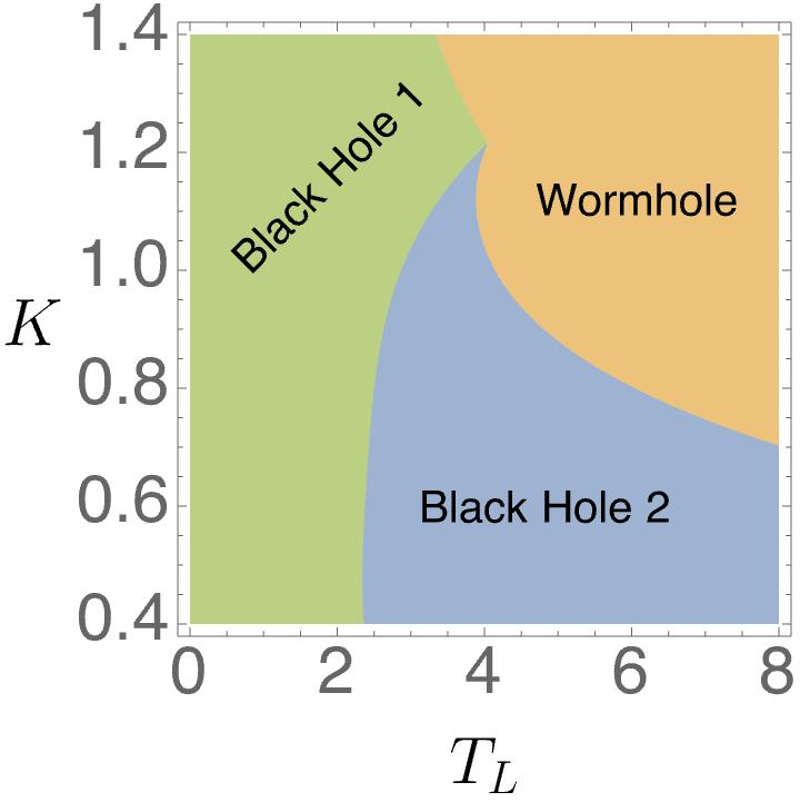
Figure 8: Dynamical phase diagram of the SYK Lindbladian with the random quadratic jump operators in terms of time $T_{L}$ and dissipation strength $K$ ($q=4,J=1$, $R=2$). The three phases are defined by $G_{++}(t)\in\mathbb{R}$, $G_{+-}(t)\equiv 0$ (green region, Black Hole 1), $G_{++}(t)\in\mathbb{C}$, $G_{+-}(t)\equiv 0$ (blue region, Black Hole 2), and $G_{++}(t)\in\mathbb{R}$, $G_{+-}(t)\not\equiv 0$ (orange region, Wormhole).

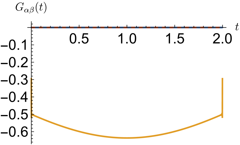
(a) $T_{L}=2$ (BH1)

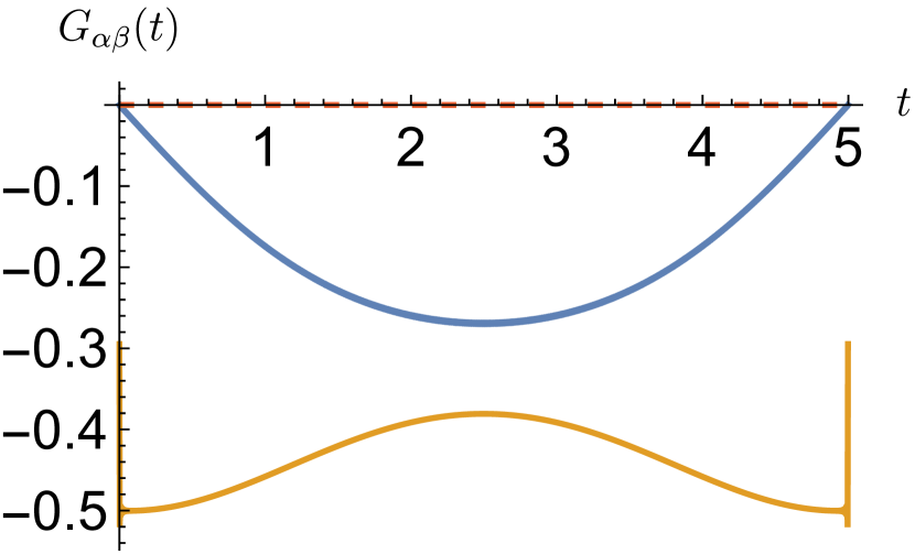
(b) $T_{L}=5$ (BH2)

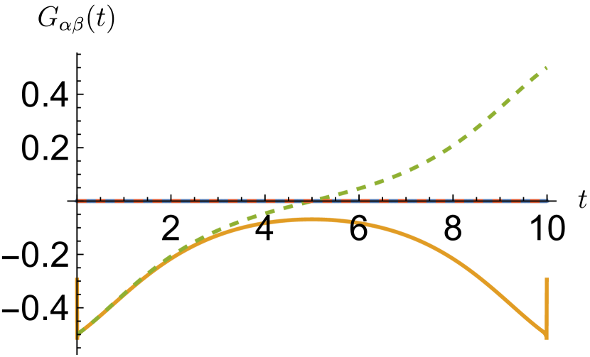
(c) $T_{L}=10$ (WH)

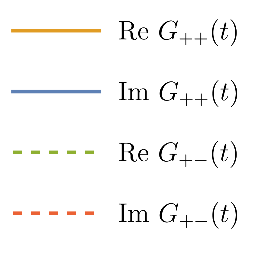
Figure 9: Representative saddle point Green’s functions $G_{++}(t)$ and $G_{+-}(t)$ in the SYK Lindbladian with the quadratic jump operators ($J=1$, $K=0.5$, and $R=2$) for (a) Black Hole 1 (BH1) phase ($T_{L}=2$), (b) Black Hole 2 (BH2) phase ($T_{L}=5$), and (c) Wormhole (WH) phase ($T_{L}=10$).

We solve the saddle point equations numerically and calculate the rate function as a function of $T_{L}$ for several values of the parameters $J,K,$ and $R$. We search for various saddle point solutions by slowly increasing (decreasing) $T_{L}$ starting from a small (large) initial value. By doing so, we obtain three kinds of saddle point solutions that correspond to three different dynamical phases , summarized as the phase diagram in Fig. 8.

Figure 9 shows the Green’s functions corresponding to these three phases. Here, we fix $J=1$, $R=2$, and $K=0.5$, and consider three different values of $T_{L}$. First, Fig. 9 (a) shows the Green’s functions at $T_{L}=2$, characteristic of the early time phase. In this phase, the same-sector Green’s functions, namely $G_{++}(t)$ and $G_{--}(t)$, are non-zero but purely real. The cross-sector Green’s functions $G_{-+}(t)$ and $G_{+-}(t)$ are identically zero, indicating that the $+$ and $-$ sectors are still decoupled. Next, Fig. 9 (b) shows the Green’s functions at $T_{L}=5$, characteristic of the intermediate time phase. The cross-sector Green’s functions are still zero, but the same-sector Green’s functions acquire a non-zero imaginary part. Since both phases are analogous to the black hole in the two-coupled SYK model, hence we label them as Black Hole 1 (BH1) and Black Hole 2 (BH2), respectively. Finally, Fig. 9 (c) shows the Green’s functions for $T_{L}=10$, characteristic of the late time phase. Now the cross-sector Green’s functions become non-zero, showing that the $+$ and $-$ sectors are now coupled. This phase is thus analogous to the wormhole in the two-coupled SYK model, so we label it as Wormhole (WH). Interestingly, $G_{++}(t)$ and $G_{--}(t)$ become once again purely real for the wormhole phase. As a consistency check, it is worth noting that for very large $T_{L}$, the Green’s functions relax to the steady-state Green’s functions discussed in Ref. [27].

Next, let us observe how the rate function behaves as we time evolve through the three dynamical phases. As an aside, for finite dissipation, we expect $i\mathcal{S}(T_{L})\rightarrow 0$ as $T_{L}\rightarrow\infty$ if the steady state is unique. However, in our numerics, we find a divergent piece that grows linearly at late times. In the subsequent analysis, we subtract this piece and only consider the regularized rate function defined as

$$i\mathcal{S}_{\text{reg}}(T_{L})\equiv i\mathcal{S}(T_{L})-\frac{K^{2}R}{24}T_{L}.$$ (53)

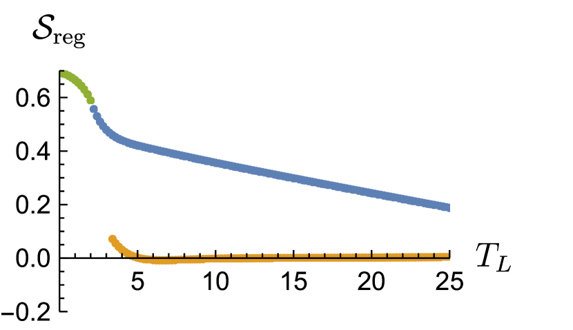
(a) $K=0.3$

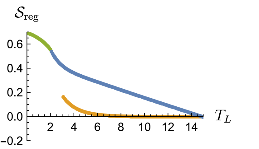
(b) $K=0.5$

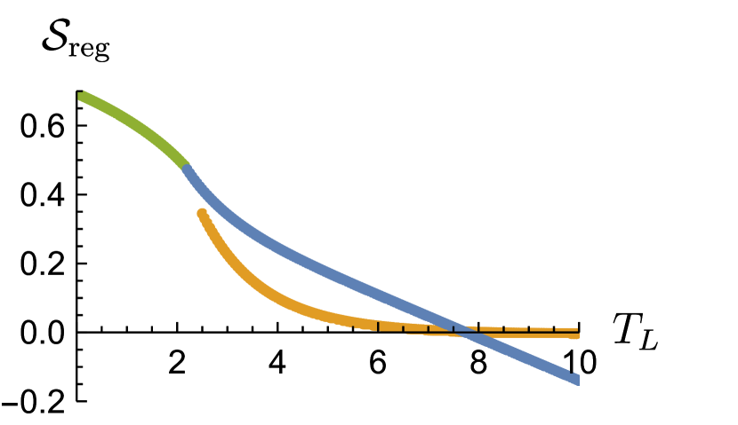
(c) $K=0.7$

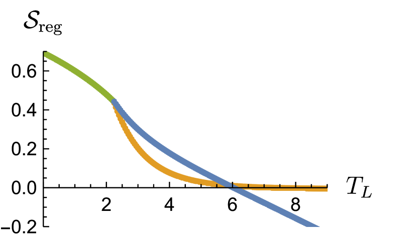
(d) $K=0.8$

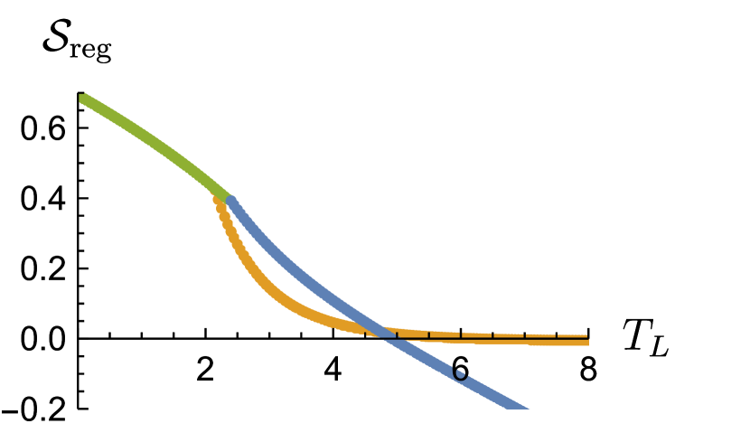
(e) $K=0.9$

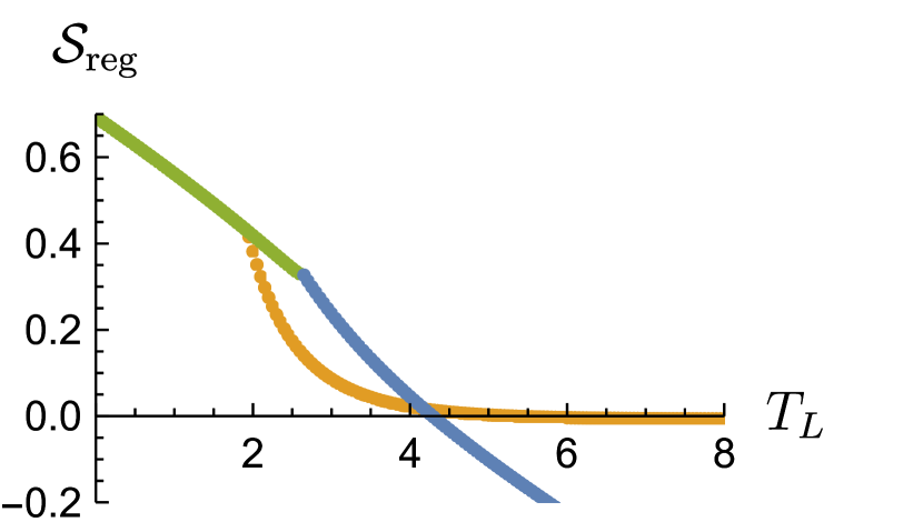
(f) $K=1$

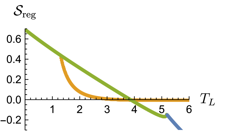
(g) $K=1.3$

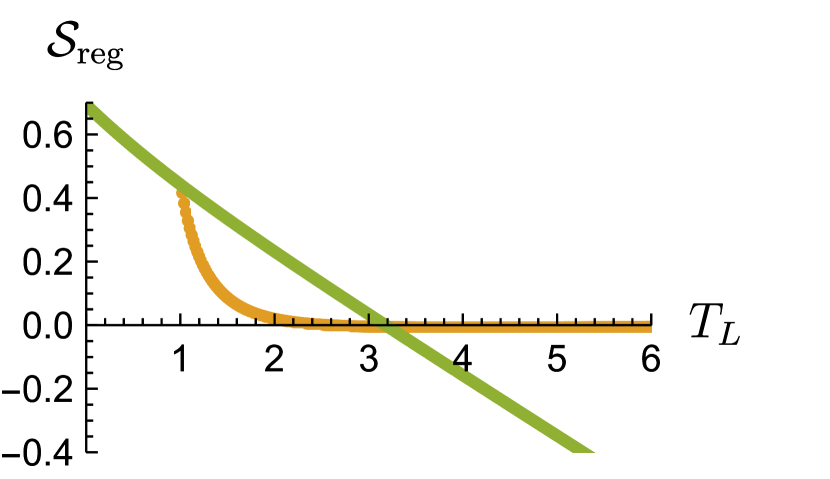
(h) $K=1.5$

Figure 10: Time evolution of the rate function in Eq. (52) for various values of the dissipative strength $K$ ($q=4,J=1$, $R=2$).

We first fix $J=1$ and $R=2$, and vary the dissipation strength $K$ from 0.3 to 1.5. The rate function as a function of time $T_{L}$ is plotted in Fig. 10. The legend shows the characterization for each phase. At every time point, the dominant phase is the one with the larger rate function. For $K\lessapprox 1.1$, all the three phases occur. The transition from early time (Black Hole 1 phase) to the intermediate time (Black Hole 2 phase) is first order for $K\gtrapprox 0.8$ and second order for $K\lessapprox 0.8$. The transition from Black Hole 2 phase to Wormhole phase is always first order. For $K\gtrapprox 1$, there are only two phases since Black Hole 2 phase (shown in blue) is always sub-dominant. We next fix $J=1$ and $K=0.3$, and vary $R$ from 5 to 30. The time evolution of the rate function is shown in Fig. 11, which exhibits similar behavior. We have the three distinct phases even for $R$ as large as $30$. The intermediate to late time transition is second order while the early to intermediate time transition is second order for $R\lessapprox 15$ and first order $R\gtrapprox 15$.

The dynamical phase diagram shown in Fig. 8 summarizes the above results. Notably, while the phase diagram for the nonrandom linear dissipators in Fig. 3 and that for the random quadratic dissipators in Fig. 8 look similar to each other, the definitions of the phases differ. Specifically, the black hole phases in the SYK Lindbladian with the linear dissipators accompany $G_{+-}\neq 0$, which contrasts with those with the quadratic dissipators satisfying $G_{+-}=0$. This difference arises from the presence or absence of fermion parity symmetry (in the strong sense [13]). On the one hand, strong fermion parity symmetry is respected in the SYK Lindbladian with the quadratic dissipators and hence can be spontaneously broken. In fact, the phase transitions between the black hole phases and the wormhole phase can be interpreted as the spontaneous breaking of strong fermion parity symmetry, in which $G_{+-}$ serves as an order parameter. On the other hand, the SYK Lindbladian with the linear dissipators explicitly breaks strong fermion parity symmetry. As a result, we generally have $G_{+-}\neq 0$ in all the phases, and the phase transitions cannot be understood as spontaneous symmetry breaking.

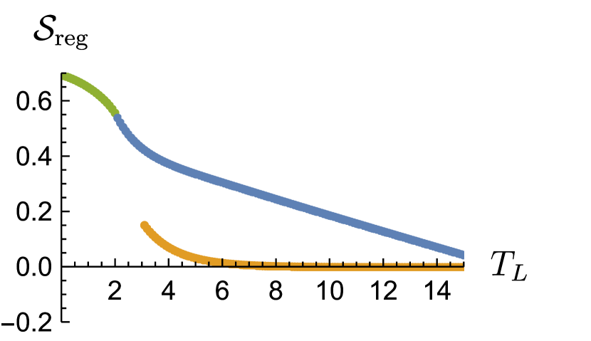
(a) $R=5$

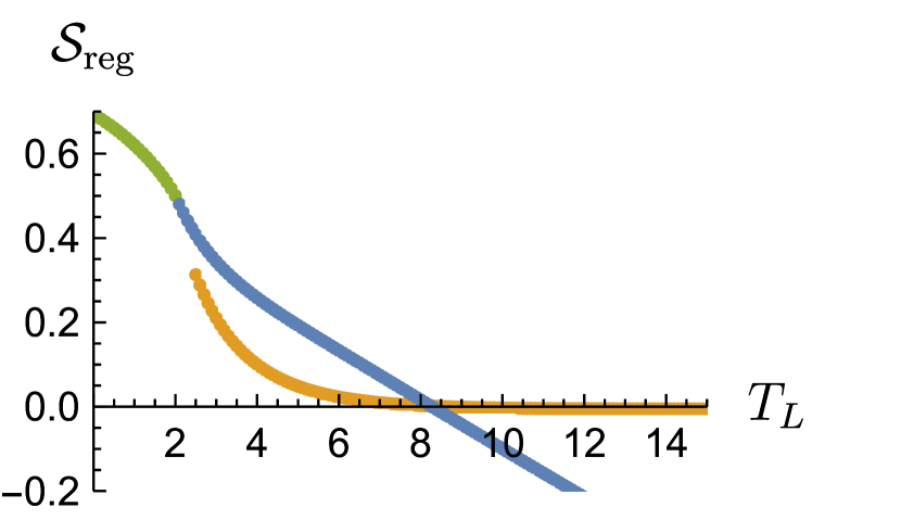
(b) $R=10$

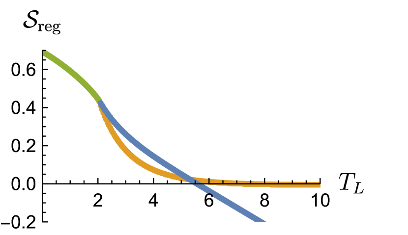
(c) $R=15$

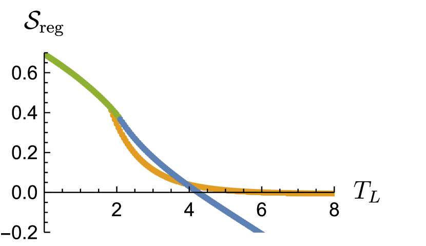
(d) $R=20$

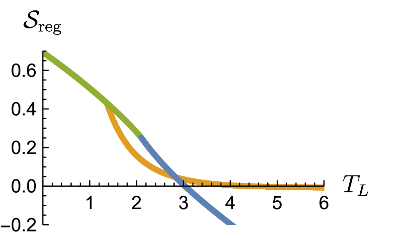
(e) $R=30$

Figure 11: Time evolution of the rate function in Eq. (52) for various values of the dissipative strength $R$ ($q=4,J=1$, $K=0.3$).

V Discussion

In this work, we have investigated the open quantum dynamics of the SYK Lindbladians and found the dynamical quantum phase transitions of its dissipative form factor. For the nonrandom linear dissipators, we have found both discontinuous and continuous dynamical phase transitions. While the former is formally analogous to the thermal phase transition in the two-coupled SYK model, the latter does not have a Hermitian counterpart. For the random quadratic dissipators, we have found the continuous phase transition that has no counterparts in the original SYK model. More precise characterizations of these phase transitions are still lacking and are left as a future problem.

More broadly, there are many open questions in the far-from-equilibrium properties of open quantum many-body systems. We expect that the SYK Lindbladians studied in this work, and generalizations thereof, can be further investigated as a prototype of open quantum many-body systems. For example, it would be interesting to calculate the dissipative spectral form factor [54, 69, 70], which may better capture the complex-spectral correlations of non-Hermitian operators. It is also notable that the operator growth has recently been studied in generic open quantum systems [71, 72, 73]. Since the SYK Lindbladians should be a prototype for the dissipative quantum chaos, it is worthwhile studying their operator growth.

Note added. While finalizing the manuscript, Ref. [74] appeared on arXiv, which has a substantial overlap with the current work. We also note another related work [75] that appeared after the submission of this work.

References

- Breuer and Petruccione [2007] H.-P. Breuer and F. Petruccione, The Theory of Open Quantum Systems (Oxford University Press, Oxford, 2007).
- Verstraete et al. [2009] F. Verstraete, M. M. Wolf, and J. I. Cirac, Quantum computation and quantum-state engineering driven by dissipation, Nat. Phys. 5, 633 (2009).
- Diehl et al. [2008] S. Diehl, A. Micheli, A. Kantian, B. Kraus, H. P. Büchler, and P. Zoller, Quantum states and phases in driven open quantum systems with cold atoms, Nat. Phys. 4, 878 (2008).
- Diehl et al. [2011] S. Diehl, E. Rico, M. A. Baranov, and P. Zoller, Topology by dissipation in atomic quantum wires, Nat. Phys. 7, 971 (2011).
- Bergholtz et al. [2021] E. J. Bergholtz, J. C. Budich, and F. K. Kunst, Exceptional topology of non-Hermitian systems, Rev. Mod. Phys. 93, 015005 (2021).
- Yang and Lee [1952] C. N. Yang and T. D. Lee, Statistical Theory of Equations of State and Phase Transitions. I. Theory of Condensation, Phys. Rev. 87, 404 (1952).
- Lee and Yang [1952] T. D. Lee and C. N. Yang, Statistical Theory of Equations of State and Phase Transitions. II. Lattice Gas and Ising Model, Phys. Rev. 87, 410 (1952).
- Fisher [1978] M. E. Fisher, Yang-Lee Edge Singularity and Field Theory, Phys. Rev. Lett. 40, 1610 (1978).
- Caldeira and Leggett [1981] A. O. Caldeira and A. J. Leggett, Influence of dissipation on quantum tunneling in macroscopic systems, Phys. Rev. Lett. 46, 211 (1981).
- Caldeira and Leggett [1983] A. O. Caldeira and A. J. Leggett, Quantum tunnelling in a dissipative system, Ann. Phys. 149, 374 (1983).
- Leggett et al. [1987] A. J. Leggett, S. Chakravarty, A. T. Dorsey, M. P. A. Fisher, A. Garg, and W. Zwerger, Dynamics of the dissipative two-state system, Rev. Mod. Phys. 59, 1 (1987).
- Bender and Boettcher [1998] C. M. Bender and S. Boettcher, Real Spectra in Non-Hermitian Hamiltonians Having Symmetry, Phys. Rev. Lett. 80, 5243 (1998).
- Albert and Jiang [2014] V. V. Albert and L. Jiang, Symmetries and conserved quantities in Lindblad master equations, Phys. Rev. A 89, 022118 (2014).
- Lee and Chan [2014] T. E. Lee and C.-K. Chan, Heralded Magnetism in Non-Hermitian Atomic Systems, Phys. Rev. X 4, 041001 (2014).
- Minganti et al. [2018] F. Minganti, A. Biella, N. Bartolo, and C. Ciuti, Spectral theory of Liouvillians for dissipative phase transitions, Phys. Rev. A 98, 042118 (2018).
- Dóra et al. [2019] B. Dóra, M. Heyl, and R. Moessner, The Kibble-Zurek mechanism at exceptional points, Nat. Commun. 10, 2254 (2019).
- Hayata et al. [2023] T. Hayata, Y. Hidaka, and A. Yamamoto, Dissipation-induced dynamical phase transition in postselected quantum trajectories, Prog. Theor. Exp. Phys. 2023, 023I02 (2023).
- Chan et al. [2019] A. Chan, R. M. Nandkishore, M. Pretko, and G. Smith, Unitary-projective entanglement dynamics, Phys. Rev. B 99, 224307 (2019).
- Skinner et al. [2019] B. Skinner, J. Ruhman, and A. Nahum, Measurement-Induced Phase Transitions in the Dynamics of Entanglement, Phys. Rev. X 9, 031009 (2019).
- Li et al. [2018] Y. Li, X. Chen, and M. P. A. Fisher, Quantum Zeno effect and the many-body entanglement transition, Phys. Rev. B 98, 205136 (2018).
- Li et al. [2019] Y. Li, X. Chen, and M. P. A. Fisher, Measurement-driven entanglement transition in hybrid quantum circuits, Phys. Rev. B 100, 134306 (2019).
- Choi et al. [2020] S. Choi, Y. Bao, X.-L. Qi, and E. Altman, Quantum Error Correction in Scrambling Dynamics and Measurement-Induced Phase Transition, Phys. Rev. Lett. 125, 030505 (2020).
- Gullans and Huse [2020] M. J. Gullans and D. A. Huse, Dynamical Purification Phase Transition Induced by Quantum Measurements, Phys. Rev. X 10, 041020 (2020).
- Sachdev and Ye [1993] S. Sachdev and J. Ye, Gapless spin-fluid ground state in a random quantum Heisenberg magnet, Phys. Rev. Lett. 70, 3339 (1993).
- Kitaev [2015] A. Kitaev, A simple model of quantum holography (2015), KITP Program: Entanglement in Strongly-Correlated Quantum Matter.
- Sá et al. [2022] L. Sá, P. Ribeiro, and T. Prosen, Lindbladian dissipation of strongly-correlated quantum matter, Phys. Rev. Research 4, L022068 (2022).
- Kulkarni et al. [2022] A. Kulkarni, T. Numasawa, and S. Ryu, Lindbladian dynamics of the Sachdev-Ye-Kitaev model, Phys. Rev. B 106, 075138 (2022).
- Gorini et al. [1976] V. Gorini, A. Kossakowski, and E. C. G. Sudarshan, Completely positive dynamical semigroups of ‐level systems, J. Math. Phys. 17, 821 (1976).
- Lindblad [1976] G. Lindblad, On the generators of quantum dynamical semigroups, Commun. Math. Phys. 48, 119 (1976).
- Liu et al. [2021] C. Liu, P. Zhang, and X. Chen, Non-unitary dynamics of Sachdev-Ye-Kitaev chain, SciPost Phys. 10, 048 (2021).
- García-García et al. [2022a] A. M. García-García, Y. Jia, D. Rosa, and J. J. M. Verbaarschot, Dominance of Replica Off-Diagonal Configurations and Phase Transitions in a Symmetric Sachdev-Ye-Kitaev Model, Phys. Rev. Lett. 128, 081601 (2022a).
- Zhang et al. [2021] P. Zhang, S.-K. Jian, C. Liu, , and X. Chen, Emergent Replica Conformal Symmetry in Non-Hermitian Chains, Quantum 5, 579 (2021).
- Jian et al. [2021] S.-K. Jian, C. Liu, X. Chen, B. Swingle, and P. Zhang, Measurement-Induced Phase Transition in the Monitored Sachdev-Ye-Kitaev Model, Phys. Rev. Lett. 127, 140601 (2021).
- García-García et al. [2022b] A. M. García-García, L. Sá, and J. J. M. Verbaarschot, Symmetry Classification and Universality in Non-Hermitian Many-Body Quantum Chaos by the Sachdev-Ye-Kitaev Model, Phys. Rev. X 12, 021040 (2022b).
- Polchinski and Rosenhaus [2016] J. Polchinski and V. Rosenhaus, The spectrum in the Sachdev-Ye-Kitaev model, J. High Energ. Phys. 2016 (4), 1.
- Maldacena and Stanford [2016] J. Maldacena and D. Stanford, Remarks on the Sachdev-Ye-Kitaev model, Phys. Rev. D 94, 106002 (2016).
- Gu et al. [2017] Y. Gu, X.-L. Qi, and D. Stanford, Local criticality, diffusion and chaos in generalized Sachdev-Ye-Kitaev models, J. High Energ. Phys. 2017 (5), 125.
- Cotler et al. [2017] J. S. Cotler, G. Gur-Ari, M. Hanada, J. Polchinski, P. Saad, S. H. Shenker, D. Stanford, A. Streicher, and M. Tezuka, Black holes and random matrices, J. High Energ. Phys. 2017 (5), 118.
- Song et al. [2017] X.-Y. Song, C.-M. Jian, and L. Balents, Strongly Correlated Metal Built from Sachdev-Ye-Kitaev Models, Phys. Rev. Lett. 119, 216601 (2017).
- Rosenhaus [2019] V. Rosenhaus, An introduction to the SYK model, J. Phys. A 52, 323001 (2019).
- Chowdhury et al. [2022] D. Chowdhury, A. Georges, O. Parcollet, and S. Sachdev, Sachdev-Ye-Kitaev models and beyond: Window into non-Fermi liquids, Rev. Mod. Phys. 94, 035004 (2022).
- Grobe et al. [1988] R. Grobe, F. Haake, and H.-J. Sommers, Quantum Distinction of Regular and Chaotic Dissipative Motion, Phys. Rev. Lett. 61, 1899 (1988).
- Xu et al. [2019] Z. Xu, L. P. García-Pintos, A. Chenu, and A. del Campo, Extreme Decoherence and Quantum Chaos, Phys. Rev. Lett. 122, 014103 (2019).
- Hamazaki et al. [2019] R. Hamazaki, K. Kawabata, and M. Ueda, Non-Hermitian Many-Body Localization, Phys. Rev. Lett. 123, 090603 (2019).
- Denisov et al. [2019] S. Denisov, T. Laptyeva, W. Tarnowski, D. Chruściński, and K. Życzkowski, Universal Spectra of Random Lindblad Operators, Phys. Rev. Lett. 123, 140403 (2019).
- Can et al. [2019] T. Can, V. Oganesyan, D. Orgad, and S. Gopalakrishnan, Spectral Gaps and Midgap States in Random Quantum Master Equations, Phys. Rev. Lett. 123, 234103 (2019).
- Can [2019] T. Can, Random Lindblad dynamics, J. Phys. A 52, 485302 (2019).
- Hamazaki et al. [2020] R. Hamazaki, K. Kawabata, N. Kura, and M. Ueda, Universality classes of non-Hermitian random matrices, Phys. Rev. Research 2, 023286 (2020).
- Akemann et al. [2019] G. Akemann, M. Kieburg, A. Mielke, and T. Prosen, Universal Signature from Integrability to Chaos in Dissipative Open Quantum Systems, Phys. Rev. Lett. 123, 254101 (2019).
- Sá et al. [2020] L. Sá, P. Ribeiro, and T. Prosen, Complex Spacing Ratios: A Signature of Dissipative Quantum Chaos, Phys. Rev. X 10, 021019 (2020).
- Wang et al. [2020] K. Wang, F. Piazza, and D. J. Luitz, Hierarchy of Relaxation Timescales in Local Random Liouvillians, Phys. Rev. Lett. 124, 100604 (2020).
- Xu et al. [2021] Z. Xu, A. Chenu, T. Prosen, and A. del Campo, Thermofield dynamics: Quantum chaos versus decoherence, Phys. Rev. B 103, 064309 (2021).
- Cornelius et al. [2022] J. Cornelius, Z. Xu, A. Saxena, A. Chenu, and A. del Campo, Spectral Filtering Induced by Non-Hermitian Evolution with Balanced Gain and Loss: Enhancing Quantum Chaos, Phys. Rev. Lett. 128, 190402 (2022).
- Li et al. [2021] J. Li, T. Prosen, and A. Chan, Spectral Statistics of Non-Hermitian Matrices and Dissipative Quantum Chaos, Phys. Rev. Lett. 127, 170602 (2021).
- Heyl et al. [2013] M. Heyl, A. Polkovnikov, and S. Kehrein, Dynamical Quantum Phase Transitions in the Transverse-Field Ising Model, Phys. Rev. Lett. 110, 135704 (2013).
- Heyl [2014] M. Heyl, Dynamical Quantum Phase Transitions in Systems with Broken-Symmetry Phases, Phys. Rev. Lett. 113, 205701 (2014).
- Budich and Heyl [2016] J. C. Budich and M. Heyl, Dynamical topological order parameters far from equilibrium, Phys. Rev. B 93, 085416 (2016).
- Heyl [2015] M. Heyl, Scaling and Universality at Dynamical Quantum Phase Transitions, Phys. Rev. Lett. 115, 140602 (2015).
- Sharma et al. [2016] S. Sharma, U. Divakaran, A. Polkovnikov, and A. Dutta, Slow quenches in a quantum Ising chain: Dynamical phase transitions and topology, Phys. Rev. B 93, 144306 (2016).
- Fläschner et al. [2018] N. Fläschner, D. Vogel, M. Tarnowski, B. S. Rem, D.-S. Lühmann, M. Heyl, J. C. Budich, L. Mathey, K. Sengstock, and C. Weitenberg, Observation of dynamical vortices after quenches in a system with topology, Nat. Phys. 14, 265 (2018).
- Jurcevic et al. [2017] P. Jurcevic, H. Shen, P. Hauke, C. Maier, T. Brydges, C. Hempel, B. P. Lanyon, M. Heyl, R. Blatt, and C. F. Roos, Direct Observation of Dynamical Quantum Phase Transitions in an Interacting Many-Body System, Phys. Rev. Lett. 119, 080501 (2017).
- Zhang et al. [2017] J. Zhang, G. Pagano, P. W. Hess, A. Kyprianidis, P. Becker, H. Kaplan, A. V. Gorshkov, Z.-X. Gong, and C. Monroe, Observation of a many-body dynamical phase transition with a 53-qubit quantum simulator, Nature 551, 601 (2017).
- Hamazaki [2021] R. Hamazaki, Exceptional dynamical quantum phase transitions in periodically driven systems, Nat. Commun. 12, 5108 (2021).
- Heyl [2018] M. Heyl, Dynamical quantum phase transitions: a review, Rep. Prog. Phys. 81, 054001 (2018).
- [65] J. Maldacena and X.-L. Qi, Eternal traversable wormhole, arXiv:1804.00491 .
- Dzhioev and Kosov [2011] A. A. Dzhioev and D. S. Kosov, Super-fermion representation of quantum kinetic equations for the electron transport problem, J. Chem. Phys. 134, 044121 (2011).
- Dzhioev and Kosov [2012] A. A. Dzhioev and D. S. Kosov, Nonequilibrium perturbation theory in Liouville–Fock space for inelastic electron transport, J. Phys.: Condens. Matter 24, 225304 (2012).
- Khramtsov and Lanina [2021] M. Khramtsov and E. Lanina, Spectral form factor in the double-scaled SYK model, J. High Energ. Phys. 2021 (3), 31.
- Shivam et al. [2023] S. Shivam, A. De Luca, D. A. Huse, and A. Chan, Many-Body Quantum Chaos and Emergence of Ginibre Ensemble, Phys. Rev. Lett. 130, 140403 (2023).
- Ghosh et al. [2022] S. Ghosh, S. Gupta, and M. Kulkarni, Spectral properties of disordered interacting non-Hermitian systems, Phys. Rev. B 106, 134202 (2022).
- Bhattacharya et al. [2022] A. Bhattacharya, P. Nandy, P. P. Nath, and H. Sahu, Operator growth and Krylov construction in dissipative open quantum systems, J. High Energ. Phys. 2022 (12), 81.
- [72] C. Liu, H. Tang, and H. Zhai, Krylov Complexity in Open Quantum Systems, arXiv:2207.13603 .
- [73] T. Schuster and N. Y. Yao, Operator Growth in Open Quantum Systems, arXiv:2208.12272 .
- García-García et al. [2023a] A. M. García-García, L. Sá, J. J. M. Verbaarschot, and J. P. Zheng, Keldysh wormholes and anomalous relaxation in the dissipative Sachdev-Ye-Kitaev model, Phys. Rev. D 107, 106006 (2023a).
- García-García et al. [2023b] A. M. García-García, L. Sá, and J. J. M. Verbaarschot, Universality and its limits in non-Hermitian many-body quantum chaos using the Sachdev-Ye-Kitaev model, Phys. Rev. D 107, 066007 (2023b).