Abstract

Quantum mechanics cements the intimate relationship between the nature of light and its detection. Historically, quantum theories of photodetection have generally fallen into two categories: the first tries to determine what quantum field observable is measured when photoelectrons are detected, laying the theoretical groundwork for photodetection being possible. The second type are phenomenological theories, which take great care to model the details of specific photodetectors. In this dissertation, we fill in the gap between these two models in the modern literature on photodetection by constructing a fully quantum-mechanical and sufficiently realistic model that includes all stages of the photodetection process. We accomplish this within the framework of quantum information theory using the language of positive operator valued measures (POVMs).

A POVM provides the most general description of a quantum measurement. In the context of single-photon detection, the photodetector POVM provides a complete characterization of the single-photon detector (SPD) from which all figures of merit can be calculated. Each element of the POVM is comprised of a weighted sum over single-photon state projectors. To construct SPD POVMs, we identify the states projected onto by a measurement and the associated weights. We first accomplish this for a simple time-dependent system, laying out how to efficiently project onto arbitrary single-photon states. Then, we describe the three stages of a realistic SPD: transmission, amplification, and measurement.

In the transmission stage of photodetection a photon enters a network of discrete energy levels, its energy propagating through that network and finally exiting into another output continuum of modes, a process entirely described by a single complex function. In the amplification stage of photodetection, a single excitation is amplified into a macroscopic signal via a nonlinear amplification mechanism. In the final stage, an inefficient “classical” measurement is made on the macroscopic signal. By combining these three stages we form a chain of inference from the final “click” to the input photon and construct a POVM projecting onto the input Hilbert space. Lastly, we discuss limits and tradeoffs that arise at each stage and implications for photodetection applications.

This dissertation contains previously published and unpublished material.

University of Oregon, Eugene, Oregon College of Wooster, Wooster, Ohio Doctor of Physics, 2020, University of Oregon Bachelor in Physics, Philosophy, 2015, College of Wooster, Ohio Theoretical Quantum Optics and Quantum Information Theory Graduate Teaching Assistant, University of Oregon, 2015-2019 Graduate Research Assistant, University of Oregon, 2016-2020 Science Literacy Program Fellow, University of Oregon, Fall 2017 & 2019 Adjunct Faculty Instructor, Lane Community College, 2019-2020 Northstar Project Teacher, University of Oregon 2016-2019 Queer Caucus Chair, University of Oregon GTFF, 2018-2020 LGBT+ in STEM Executive Board, University of Oregon, 2017-2020 John R. Moore Scholarship, University of Oregon, 2020 Most Informative Talk, University of Oregon Women in Graduate Science Science Slam, 2018 First Place, Oregon Statewide 3 Minute Thesis Championship, 2017 First Place, University of Oregon 3 Minute Thesis Competition, 2017 Physics Department Teaching Award, University of Oregon, 2017 Propp, Tz. B & van Enk, S. J. (2019). On nonlinear amplification: improved quantum limits for photon counting. Optics Express 27, 16, 23454-23463. Propp, Tz. B & van Enk, S. J. (2019). Quantum networks for single photon detection. Physical Review A, 100, 033836. Propp, Tz. B & van Enk, S. J. (2020). How to project onto an arbitrary single-photon wavepacket. Submitted to Physical Review A. I would like to thank my advisor Dr. Steven van Enk for his mentorship in completing this dissertation, for supporting me through the hardest years of graduate school, and for inspiring me to strive to be the best and happiest theoretical physicist I can possibly be. I also want to thank my former advisor and committee chair Dr. Ben McMorran for believing in me and helping instill in me the value of outreach, along with PhD committee member Dr. Dave Wineland for invaluable revisions. I would like to thank Andrea Goering, Brandy Todd, and Benjamín Alemán for supporting me, providing mentorship, and enabling my physics outreach endeavors. Similarly, I want to thank Dr. Elly Vandegrift who opened my eyes to the science of science education, and whose mentorship has been instrumental to my development as both teacher and learner. I would like to acknowledge the leadership of the Graduate Teaching Fellows Federation, as well as University of Oregon Lesbian, Gay, Bisexual, and Trans+ Education Support Services (LGBTESS) coordinator Haley Wilson for their institutional support. Special thanks are due to Saumya Biswas who–in his own words–did not get in the way, along with our collaborators in the DARPA DETECT program for thought-provoking discussions. I would like to acknowledge the Kalapuya tribe, on whose stolen land this research was conducted. Lastly, I want to thank my queer chosen family and friends for being there for me through the toughest times, particularly Vé Gulbransen, Hales Wilson, and Liana Clark as well as Deepika Sundarraman, Hayley Shapiro, Christianna Hannegan, Alice Greenberg, Abby Pauls, Caden Valencia, and many others. This research was supported financially in part by DARPA contract No. W911NF-17-1-0267 and the Emanuel OMQ Scholarship. blank filler text. I dedicate this dissertation to my beloved cat King Ubu who is also known as Small Bean Black Bean Moon Bean Sun Bean Bean-O’Noire Tiabanie Beanie Baby Sneaky Bean and The Bean. This dissertation is the product of unionized labor as part of the Graduate Teaching Fellows Federation, AFT Local 3544.

Chapter 1 Introduction

1.1 History

Measurements are our window to the universe. Since the ancient Greeks, we have accepted that we only have access to our perceptions, not direct access to the phusis or physical reality. The statement that we can only know what we can measure has withstood the test of time, and is now enshrined and made explicit in quantum theory’s separation of measurement and the quantum state. Yet even though no measurement can reveal the complete underlying reality (if such an underlying reality even exists), we can improve our measurements to better reveal physical reality in analogy to Plato’s famous Allegory of the Cave [1], depicted in Fig. 1.1; in quantum theory, it is as if we are trying to learn about light (the quantum state) by studying the shadows different objects cast (projective measurements). This is necessary, as there is a real sense in which our measurements constitute the most foundational layer of the universe to which we have direct access. In this way, if we wish to learn more about the structure and constituents of physical reality, our study should include consideration of our measurement schemes themselves.

Figure 1.1: Plato’s allegory of the cave [1], as illustrated on the cover of Diagnosis: interpreting the shadows [2]. By improving our measurements, we can improve our understanding of the universe even if the ultimate level of direct access to reality (for Plato, looking directly at the sun) is unattainable.

The study of light and its measurement date back to at least $500$ to $300$ BCE [6]. These early works by Ptolemy and Euclid were preserved and expanded upon in the Islamic world with the works of Ibn Sahl on curved mirrors and lenses in $984$ CE [7], Ibn Al-Haytham on the correct identification of vision as a three-part process involving a light source, a reflected object, and the eye between $1028$ and $1038$ CE [8], and Kamāl al-Dīn al-Fārisī on the mathematically rigorous description of the rainbow phenomena in $1309$ CE [9]. These concepts were introduced to Europe during the Renaissance, where the well-developed science of spectacle construction (curved lenses) was used by Hans Lippershay in $1608$ to create the first telescope, an invention which was subsequently refined by Johannes Kepler and modified to magnify nearby objects (that is, the invention of the microscope) in the subsequent three years [10]. These developments in our ability to measure and manipulate light paved the way for a series of early experiments in the mid-1600’s, most famously by Isaac Newton and Christiaan Huygens, trying to elucidate the nature of light which was believed to be a particle by the former and a wave by the latter. These experiments were built upon in the following century and a half by Thomas Young (wave theory: interference), Etienne Louis Malus (wave theory: polarization), Augustin-Jean Fresnel (wave theory: polarization and interference), Simeon-Denis Poisson (particle theory: shadows and attempting to refute Fresnel) and Francois Arago (wave theory: diffraction and refuting Poisson). During this same time period, parallel research by Hans Christian Ørstedand and later Michael Faraday in unifying electricity and magnetism. This all culminated in the unifying work by James Clerk Maxwell, who proved in 1864 that light is an electromagnetic wave with a speed exactly determined by the electromagnetic permittivity and permeability of free space [11].

Despite the rigorous theoretical foundation of the wave theory of light and the tremendous predictive success of classical physics, the wave theory of light alone failed to explain several phenomena including the photoelectric effect and the Rayleigh–Jeans ultraviolet catastrophe for blackbody radiation. The resolution of these mysteries required the elucidation of wave-particle duality, wherein both the particle and wave properties of light are understood as differing aspects of a single quantum theory [11]. The definitive evidence for wave-particle duality was the discovery of the Compton effect in 1923, wherein an X-ray changes momentum after colliding with a target [13]. While the wave nature of light was already well established as essential to quantum theory, the Compton effect made it clear that light must not only be quantized but also exhibit the properties of classical particles as well at sufficiently small wavelengths.

The development of the modern understanding of light and its detection is simultaneous with the advent of quantum theory in the early 1900’s [14]. In the low-energy limit (that is, below $1.02MeV$ where a photon can spontaneously produce an electron and positron), it is convenient to represent light in the Fock basis so that it is comprised of photons, the quanta of the electromagnetic field. Not all quantum states of light have a definite integer number of photons, either because of unknown correlations with an environment (for instance, a thermal distribution of photons) or because of quantum necessity (for instance, coherent states of light, such as those produced by a laser). In these cases, the state projected onto is not a pure Fock state but a mixture (or a coherent superposition) of Fock states. However as the quantum degree of freedom of the electromagnetic field, any pure measurement that projects onto Fock states will only retrodict an integer number of photons even though the internal state of the photodetector may be partially unknown (mixed); that is, there may be many internal photodetector states corresponding to a single detector outcome.

The lowest non-zero integer is one, so single-photon detection is the intensity-frontier limit to detection of photon Fock states. For this reason, we expect the fundamental quantum limits to general photodetector figures of merit to be manifest in quantum descriptions of single-photon detectors (SPDs). In this dissertation, we will construct what is (to our knowledge) the first completely quantum description of the entire photodetection process in a SPD in order to identify the fundamental limits and tradeoffs inherent to single-photon detection.

In addition to the pure intellectual merit, answering the question “What are the fundamental limits to single-photon detection?” is important for industry applications of SPD-based technology. Recently, there has been progress in achieving single photon detection with unprecedented performances in standard photodetector figures of merit [19]: timing jitters or temporal uncertainties in the tens of picoseconds in superconducting nanowire SPDs [20, 21], dark count rates on the order of a single dark count per day [22, 23], and robustness to thermal fluctuations nearing room temperature performance [24, 25]. This is in no small part due to the work done by the DARPA DETECT collaboration, one of the aims of which is to jumpstart the next generation of photodetection technology. Exploration of fundamental limits and tradeoffs inherent to single-photon detection is essential to guiding this work, so experimentalists can have ideas of what they will come up against and decisions can be made about which areas of tradespace are important to explore. Furthermore, they enable accountability; if a research group claims their photodetector can simultaneously perform well in metric X and metric Y, and we know metric X and Y are not simultaneously attainable from our generic model, we have good reason to question their claims. While the DARPA DETECT collaboration has resulted in a plethora of device-specific phenomenological theories of photodetection [26, 21, 24, 27, 28], the universal limits to SPDs are not explicit in such models (even though they are present). To construct a model where the limits themselves are revealed (our goal), we must answer the following two questions: What are the essential components of an SPD? What are the fundamental limits of each component’s performance? We will answer these two questions and construct a model where the fundamental limits to SPD performance are manifest. However, it first behooves us to review photodetection theory in the modern era.

The advent of a quantum theory of photodetection is simultaneous with the advent of quantum theory, and has its origins in Einstein’s Nobel prize-winning study of the photoelectric effect [14]. Here for the first time the notion that light can only be absorbed (and thus detected) in discrete packets of energy or quanta was rigorously incorporated into the foundation of a theory, which was accomplished by building upon the more ad hoc treatment by Planck [29]. With this, Einstein was able make statistical arguments for rates of atomic transitions in the two-level approximation in the presence and absence of an external electromagnetic field. In this way, Einstein was able to describe the known processes of spontaneous emission and absorption, as well discover stimulated emission [30]. This was done without a relativistic quantum treatment of the electromagnetic field itself, the methods for which did not exist at the time. Instead, Einstein made use of knowledge of the Planck blackbody spectrum in order to demand agreement with quantum theory. In a photodetector approximated as a two level system, the Einstein rate equations are directly connected to the efficiency with which a photon is absorbed and with how long it stays in the detector before leaking back out (which can be connected to a gain factor in an amplification scheme such as electron shelving [31]).

Although Einstein was able to correctly predict the rates of emission and absorption for a two-level system, it was not until work by Dirac in 1927 (and, throughout the next two decades, Wignerl Oppenheimer, Fermi, Bloch, Weisskopf, Tomonoga, Schwinger, and Feynman) formulating a theory of quantum electrodynamics (QED) that a complete quantum treatment of the electromagnetic field interacting with matter (here, only the electron) was developed [32, 33, 34, 35, 36, 37, 38, 39, 40]. One of the key developments was a quantum treatment of the vacuum, clarifying spontaneous emission as stimulated emission due to vacuum fluctuations by Wigner and Weisskopf [41]. Another key development was a quantum method for treating the continuum of electromagnetic field modes using Dirac-normalized creation and annihilation operators. These well-known physicists, along with others, contributed to the extension of QED in the development (and predictive success) of relativistic quantum field theory, laying the foundation for modern particle physics which has dominated the popular news spotlight ever since. Meanwhile and behind the scenes, another revolution was brewing as the the initial question of an electromagnetic field interacting with matter was further explored with the new methods of QED.

In 1959, Hanbury Brown and Twiss published a controversial paper showing that, for a few-photon signal collected from the star Sirius, an interference effect was observable in intensity from which the angular size of Sirius was calculable [42]. Purcell was quick to point out that this interference can be understood as a manifestation of boson statistics applied to counting photons [43]. However, the underlying mechanism behind the Hanbury Brown-Twiss effect was partial coherence, a property of classical waves that had yet to be understood at the quantum level.

In his seminal work in 1963 [44], Glauber connected the quantized formulation of the electromagnetic field to experimentally measurable correlations using the language of QED, introducing the field intensity correlation as a measure of quantum coherence and calculating transition probabilities correlated with the detection of individual photons. We will illustrate the method now, focusing on a single polarization $\mu$ of the electromagnetic field and following [45]. The first step is to separate the quantized (that is, operator-valued) electric field into positive and negative frequency components

$$\hat{E}_{\mu}(\vec{r},t)=\hat{E}_{\mu}^{+}(\vec{r},t)+\hat{E}_{\mu}^{-}(\vec{r},t)$$ (1.1)

where $\mu$ denotes the polarization we are describing and we note $\hat{E}_{\mu}^{+}(\vec{r},t)^{\dagger}=\hat{E}_{\mu}^{-}(\vec{r},t)$. We can represent the operator $\hat{E}_{\mu}^{+}(\vec{r},t)$ as a sum over discrete plane wave modes with frequencies $\omega_{j}$

$$\hat{E}_{\mu}^{+}(\vec{r},t)=-\sum_{j}\sqrt{\frac{\hbar\omega_{j}}{2\epsilon_{0}}}e^{\vec{k}_{j}\cdot\vec{r}-i\omega_{j}t}\hat{\epsilon}_{\mu}\hat{a}_{j}$$ (1.2)

with $\hat{\epsilon}_{\mu}$ the component of the polarization vector, $\vec{k}_{j}=\vec{p}/\hbar$ the wave number proportional to the momentum $\vec{p}$, $\epsilon_{0}$ the permittivity of free space, $\hbar$ Planck’s reduced constant, $i=\sqrt{-1}$, and $\hat{a}_{j}$ the annihilation operator corresponding to the mode $j$. Since $[\hat{a}_{j},\hat{a}^{\dagger}_{j}]=1$, the positive and negative electric field components will not commute. We can associate a photodetection event with a transition in the state of the field $\left|i\right\rangle\rightarrow\left|f\right\rangle$. For idealized single photon detection, the difference between the initial and final state is that one photon in mode $j$ was removed through an interaction at location $\vec{r}$ and time $t$. For each particular initial field configuration, the transition probability is described by unitary evolution

$$\left\langle f\right|\hat{U}(i\rightarrow f)\left|i\right\rangle \propto \left\langle f\right|\hat{E}_{\mu}^{+}(\vec{r},t)\left|i\right\rangle$$ (1.3)

$$\propto \left\langle i\right|\hat{E}_{\mu}^{-}(\vec{r},t)\hat{E}_{\mu}^{+}(\vec{r},t)\left|i\right\rangle$$

where proportionality with the full sum in (1.2) achieved due to only a single term contributing to the to the matrix element and the sum over polarizations $\mu$ is implicit. Since the initial state $\left|i\right\rangle$ is arbitrary, we can carry out a sum over initial states and perform an average so that the full transition probability is proportional to

$$P(t)\propto\langle\hat{E}_{\mu}^{-}(\vec{r},t)\hat{E}_{\mu}^{+}(\vec{r},t)\rangle$$ (1.4)

where the angled brackets indicate an average or expectation value. This expression for the photodetection probability motivated Glauber to define a field correlation function. (1.4) is a special case of the first-order coherence

$$G^{(1)}(\vec{r}_{1},t_{1};\vec{r}_{2},t_{2})=\langle\hat{E}_{\mu}^{-}(\vec{r}_{1},t_{1})\hat{E}_{\mu}^{+}(\vec{r}_{2},t_{2})\rangle$$ (1.5)

By rewriting the electric field in terms of positive and negative frequency components promoted to operators, Glauber was able to calculate measures or degrees of coherence of the quantum field in terms of a series of coherence functions, each measuring correlations at some order of the electric field operators. Both (1.4) and (1.5) are normally ordered, so that, for the vacuum state, $P(t)=G^{(1)}(\vec{r}_{1},t_{1};\vec{r}_{2},t_{2})=0$. First-order coherence described by (1.5) is analogous to classical coherence in standard optics, but Glauber showed that quantum systems can also exhibit higher order correlations and coherences, making rigorous the theoretical foundation for the maser and laser. Critically, Glauber also introduced the coherent state representation for quantum states. These coherent states are minimum uncertainty states in the quantum field quadratures and are denoted by a single complex number identifying both the amplitude and phase of the electromagnetic field (which are precisely what defines a particular laser field). As the “most classical” states, the coherent states form a bridge between quantum and classical descriptions of light.

To this day, the Glauber model of photodetection, given in terms of field correlations and point-like interactions between a quantized electromagnetic signal and a photoionization system (or other quantum electrical system) as in (1.4), provides the foundation for modern photodetection theory. Although it is mathematically rigorous, the Glauber model is highly idealized as a practical theory of measurement; critically, Glauber merely posits that one is able to count photoelectrons without describing any subsequent mechanisms. This work was soon expanded to incorporate less-idealized descriptions of the electromagnetic field-photodetection interaction [46, 47], with later additions to the theory also incorporating the back action of the detector on the detected quantum field [48, 49, 50, 51, 52]. Throughout, a challenge to photodetection theory has been describing the interaction between a discrete system (from a photon’s perspective, a system of discrete bosonic states) and the full continuum of bosonic states of the electromagnetic field. In the intermediate years, numerous quantum optical techniques have been developed for describing the continuum of states, some of which we will discuss in detail in the next chapter.

We will end this section with a brief survey of modern photodetecting platforms amenable to single photon detection. (For in-depth review, see Refs. [19, 54].)

Photoionization, the production of a current due to incident radiation, is the method of photodetection longest studied quantum mechanically and has as its fundamental theory the photoelectric effect [55]. First constructed by Hertz in 1887 [56], the photomultiplier tube (PMT) is a cathode and vacuum-tube device that uses the photoelectric effect coupled with secondary emission to amplify signals as small as an single incident photon into a macroscopic signal. Despite its quantum mechanical foundation and use in counting photons, it is possible to generate a “classical” theory of a PMT where the external quantum field is treated as a perturbation to which the PMT responds, achieving a new steady-state. In this case, it is straightforward to calculate the statistics of photodetection events [46]; the probability of detecting $n$ photons between a time $t$ and $T$ is calculated

$$P(n,t,T)=\int_{0}^{\infty}\frac{1}{n!}W^{n}e^{-W}{\cal P}(W)dW$$ (1.6)

with

$$W=\eta\int_{t}^{t+T}I(t^{\prime})dt^{\prime}$$ (1.7)

where $\eta$ is the photodetection efficiency, $I(t)$ is the intensity of the electromagnetic field, and ${\cal P}(W)$ is the quasi-probability distribution of the integrated intensity. While highly idealized, this expression can be included into more realistic semiclassical models [57], and alone rapidly gives useful predictions (even for a somewhat generic photodetector). For instance, for a thermal distribution of light one finds that (1.6) yields a Bose-Einstein distribution for photodetection events [55]. However, this semiclassical formula does not describe the truly quantum nature of multi-photon detection as made explicit in Hanburry Brown and Twiss’ work [42].

Another widespread SPD platform is the avalanche photodiode (APD), invented by Jun-ichi Nishizawa in 1952 [58]. Like the PMT, APDs function based on the photoelectric effect. Whereas in an light-emitting diode (LED) electrons and holes annihilate converting current into light, in an APD an incident photon with energy greater than the material band gap generates an electron-hole pair, resulting in a current [59]. Generally, APDs can only operate in single-photon detection mode at the expense of significant reset or dead time as the circuit must be quenched unless an array is used [59, 60], so for an individual APD pixel within an array Mandel’s formula (1.6) only applies for $n\leq 1$ (higher order counts are highly suppressed). However, for single photon detection we are indeed interested in the $n\leq 1$ regime and Mandel’s formula will have validity.

Other single photon detecting platforms are less straightforward, but all share a generic feature; the presence of a photon changes the state of the system, either by shifting the equilibrium state or temporarily moving the system out of equilibrium. Examples of the former include quantum dot field transistor detectors [61] and superconducting transition-edge sensors (TES) [62], both of which involve a measurable change in system conductance due to absorption of a photon. (It is especially drastic for TES, the system is taken out of the superconducting state!) Since the equilibrium state has changed, resetting these mechanisms is resource intensive and SPDs built on these principles have a longer dead time ($\sim 10\mu s$) compared to newer technologies [19]. An interesting example of temporarily moving a system out of equilibrium are superconducting nanowire single photon detectors (SNSPDs) [63, 22, 23, 64], which in recent years have seen a rising popularity due to their low dark count rates ($\sim 10Hz$) and dead times ($\sim 1ns$). However, while theoretical modeling based on time-dependent Ginzburg-Landau theory has produced qualitative agreement with experiment, quantitate models for SNSPDs remain elusive [65]. In part, this is due to the complexity of system dynamics; in an SNSPD a photon is collectively absorbed by many electrons and phonons, resulting in a hot spot in which vortex anti-vortex pairs form with local variations in the superconductivity. This results in a measurable voltage when the vortex anti-vortex pair crosses the wire.

It is worth noting that one method of detecting single photons has been around for thirty million years, namely, the African clawed frog Xenopus laevis [66]. This species can detect single photons of visible light with moderate ($\leavevmode\nobreak\ 30\%$) efficiency and, as living organisms, they do this at room temperature. This has motivated other participants in the DARPA DETECT program to develop bio-inspired SPD platforms [25]. Although these will suffer from larger dark count rates due to the increased thermal noise at higher temperatures, the hope is that they still may have high enough signal-to-noise ratio to be useful in room temperature experiments.

1.2 Very Brief Introduction to Quantum Information and POVMs

During the late 20th century and on into the 21st century, a revolution has been taking place in quantum science; technological advancements are allowing for increasing control over environmentally isolated single quantum systems [67, 68, 69, 70, 71, 72, 73, 74, 75, 76, 77, 78]. Simultaneously, physicists were increasingly realizing the limits of classical computation both in terms of scalability and applicability to quantum systems [79]; Moore’s law describing the size of transistors must break down when we approach the size of single atoms. And if we are interested in simulating quantum systems, shouldn’t we utilize a quantum system itself to do so [79]? Early pioneers of quantum information science were quick to discover problems where a quantum algorithm provided an exponential speedup [80, 81] and the so-called second quantum revolution was born [75]. In many quantum algorithms, an essential ingredient is measurement of an internal two-level system or qubit whose state encodes information (generically, the answer to some input query with some known probability). Thus the need for measurement theory, the rigorous theoretical foundation for describing quantum measurement.

Measurement is a ubiquitous concept in quantum theory: examples include measurements of an electron’s position or momentum (limits to the simultaneous performance of which are enforced by Heisenberg’s uncertainty principle [82]), measurement of the population of a multi-level system (such as an atom, simple harmonic oscillator, optical cavity, or quantum dot), or detection of light through the use of a photo detector (as we will explore in this thesis). The most general quantum description of a measurement is in terms of a positive operator-valued measure (POVM), a set of positive operators $\hat{\Pi}_{k}$ that sum to the identity, where each $k$ corresponds to a different measurement outcome. Given an arbitrary quantum state $\hat{\rho}$ the probability to obtain outcome $k$ is given by the Born rule

$$P(k)={\rm Tr}(\hat{\rho}\hat{\Pi}_{k})$$ (1.8)

where ${\rm Tr}(\hat{O})$ is the trace of the operator $\hat{O}$.

Generically, each POVM element $\hat{\Pi}_{k}$ can be written as a weighted sum over projectors onto orthogonal quantum states

$$\hat{\Pi}_{k}=\sum_{i}w_{i}^{(k)}\left|\phi_{i}^{(k)}\right\rangle\left\langle\phi_{i}^{(k)}\right|$$ (1.9)

reducing to an ideal projective von Neumann measurement only when the sum reduces to a single term with its weight $w^{(k)}$ equal to unity [83]. The weight $w_{i}^{(k)}$ equals the conditional probability to obtain measurement outcome $k$ given input state $\left|\phi_{i}^{(k)}\right\rangle$. The posterior conditional probability that, given an outcome $k$, we project onto input $i$ is given by Bayes’ theorem [84]

$$P(i|k)=\frac{w_{i}^{(k)}P(i)}{P(k)}$$ (1.10)

with $P(k)=\sum_{i}w_{i}^{(k)}$. Here, $P(k)$ is a priori probability for observing measurement outcome $k$, and and $P(i)$ is the a priori probability for the $i$th input state $\left|\phi_{i}^{(k)}\right\rangle$ to be present [85]. Through Bayes’ theorem, an experimentalist is able to retrodict the likely input state or states; they can update the probability distribution over the possible (past) inputs if and only if they know what measurement they actually perform.

In the next chapter, we discuss applications of POVMs to single-photon detection. First, we will review general properties of POVMs in the remainder of this section, before giving an overview of the structure, format, and goals of this dissertation in the final section of this chapter.

The POVM has several interesting properties it is worthwhile to review and note: firstly, a POVM forms a partition of unity. If one sums over all measurement outcomes (including the null outcome), from the Born rule one finds $\sum_{k}{\rm Tr}(\hat{\rho}\hat{\Pi}_{k})=1$ for any state $\hat{\rho}$; in other words, regardless of the input quantum state we can be sure that some outcome will occur since the probabilities of all outcomes necessarily sum to unity!

Although the POVM is a complete description of a measurement, we note that alone it is insufficient to determine the post-measurement quantum state. For this we must additionally define Kraus operators $\hat{A}_{k}$ satisfying $\hat{A}_{k}^{\dagger}\hat{A}_{k}=\hat{\Pi}_{k}$ [85]. Note that the POVM does not uniquely specify $\hat{A}_{k}$, as for any unitary $\hat{U}$ the substitution $\hat{A}_{k}\rightarrow\hat{U}\hat{A}_{k}$ leaves the POVM unchanged. Having defined Kraus operators, the normalized post-measurement state $\hat{\rho}^{\prime}$ is calculated

$$\hat{\rho}^{\prime}=\frac{\hat{A}_{k}\hat{\rho}\hat{A}_{k}^{\dagger}}{{\rm Tr}(\hat{A}_{k}\hat{\rho}\hat{A}_{k}^{\dagger})}.$$ (1.11)

We note that repeated measurement will not guarantee the same outcome (unless the measurements are von Neumann measurements), as the measurement outcomes are not orthogonal.

Non-orthogonality is a general feature of POVM elements (except in the case of the idealized von Neumann measurement, which always project onto orthogonal [and pure] quantum states). Of particular interest in quantum information theory are symmetric, informationally complete (SIC)-POVMs; the POVM is considered symmetric if each of the elements of these POVMs share the same mutual overlap ${\rm Tr}(\hat{\Pi_{i}}\hat{\Pi_{j}})=\frac{d\delta_{ij}+1}{d+1}$ with $d$ the dimension of the Hilbert space and $\delta_{ij}$ the Kronecker delta ($0$ when the indices are not the same, unity when the indices are the same). Additionally, the SIC-POVM is informationally complete if there are $d^{2}$ elements in the POVM, where $d^{2}-1$ are linearly independent. While they will not be discussed further in this dissertation, they are of particular importance to two applications of our work which we will discuss, quantum state tomography [86] and quantum cryptography [87], where they illuminate the most efficient measurement scheme for quantum state characterization. Furthermore, there are interesting connections to be made between SIC-POVMs and mutually unbiased bases of quantum states, with the latter playing an essential role in quantum communication and cryptographic protocols [88].

1.3 Overview and Glossary

Having laid the theoretical foundation for our work in this first chapter, we now review the structure of this dissertation. We also provide a glossary of terms ubiquitous in this thesis at the end of this section (see Tbl. LABEL:glossary).

The motivation and goal of this work is to uncover the fundamental limits inherent to single photon detection across physical platforms, both current and future. To accomplish this, we approach photodetection from the perspective of information theory, recasting the process of detecting a photon into the interpretation of a photodetection outcome in the absence of priors. Interpretation of a measurement outcome requires sufficient information about the measurement apparatus to identify the POVM implemented. As such, it is necessary to develop a model of photodetection that is realistic in describing all parts of the photodetection process, but sufficiently idealized and general so that the limits to each part of the process are fundamental limits across all platforms.

In the next chapter of this dissertation, we begin the construction of such a model starting with a POVM corresponding to the time-dependent two-level system. Here a detection event occurs when one “checks” whether the two-level system is in the excited state at a particular time $T$. The two-level system is an essential component to a description of an SPD, as it ensures the measurement projects onto the Hilbert space of single-photon states. As we show, the time-dependent nature of this system is sufficient to project onto arbitrary single-photon wavepackets (with arbitrarily high efficiency), including Gaussian wavepackets so that Heisenberg-limited simultaneous measurements of time and frequency are implemented. At the end of the second chapter, we introduce our three-stage model of the photodetection process: transmission, amplification, and measurement (Fig. 2.4), and clarify the role of the time-dependent two-level system in this model as the trigger for the amplification mechanism.

In the third chapter of this dissertation, we analyze transmission functions $T(\omega)$ describing the quantum network structure of the transmission stage of photodetection. In the transmission stage, the photon has to interact with one or more charged particles, its excitation energy will be converted into other forms of energy which will later lead to a macroscopic signal. In this chapter, we discuss the tradeoffs inherent to different network structures and their implications for photodetecting systems.

In the fourth chapter of this dissertation, we analyze the amplification process itself. In particular, we identify commutator-preserving transformations that implement different nonlinear amplification schemes outperforming linear amplification in terms of signal-to-noise ratios (SNRs) as illustrated in Fig. 4.2. Additionally, we demonstrate that amplification into a single bosonic mode not only outperforms all previously analyzed amplification schemes, but provides the fundamental limit to amplification of single and many-photon Fock states.

In the fifth chapter of this dissertation, we introduce the final measurement stage and construct realistic SPD POVMs that include all three stages of photodetection. In particular, we demonstrate that an SPD POVM retrodicts a relatively pure external state of the electromagnetic field, even though the internal state of the detector is highly mixed in general. In the remainder of this chapter, we discuss applications to quantum cryptographic protocols, quantum sensing, and quantum information science.

In the sixth and final chapter of this dissertation, we discuss the fundamental limits and tradeoffs inherent to photodetection encapsulated by the three-stage model of photodetection. We also discuss implications of this work for the future development of novel SPD platforms.

Chapter 2 POVMs for Single-Photon Detection

In this chapter, we review techniques in quantum information theory amenable to single-photon detection, in particular, the definition of photodetector figures of merit. Then, we construct a simplified single-photon detector (SPD) positive operator valued measures (POVM) capable of projecting onto arbitrary single-photon wavepackets. Lastly, we discuss the three stages of photodetection universal to all detector schemes, each of which we will analyze in detail in its own chapter.

2.1 Quantum Information for Photodetection

Photodetection is at its core an information theoretic process; a measurement outcome—a click—reveals information about the outside world quantifiable in bits [90]. In the case of a single-photon detector (SPD), a click is correlated (imperfectly) with the presence of a photon in a particular single-photon state. (Here, the quantum state refers to the spectral, spin angular momentum, and orbital angular momentum quantum degrees of freedom at every point in spacetime). In this way, a detection reveals information about the presence of photons in that particular state, along with whatever else in the world is correlated with that photon state. For an example from fluorescence microscopy, detection of ultraviolet light when a sample is illuminated with red light is positively correlated with the presence of fluorine [91]. For single photons, measurements that detect light are naturally described through a SPD POVM.

Knowledge of the POVM is essential for both gaining information from a measurement device and characterizing detector performance, hence the experimental need for detector tomography [92, 93, 94, 95, 96, 97]. In detector tomography, known quantum states are input to a device to determine the quantum states projected onto by different outcomes (along with their associated weights) and calculate the full measurement POVM. Commercial photodetectors are characterized by industry-standard figures of merit [19], which can be calculated from a POVM (for an in-depth review, see Ref. [98]). Here we will concern ourselves mostly with two standard figures of merit, detection efficiency and time-frequency uncertainty:

Efficiency.—The maximum efficiency with which an SPD outcome $k$ (for instance, a single click) can be triggered by input single-photon states is exactly the maximum relative weight in (1.9): $\eta_{\max}={\rm Max}_{i}[w_{i}^{(k)}]$. This maximum efficiency is achieved only when the input quantum state is the single-photon state the measurement maximally projects onto. This follows directly from the Born rule; $P(k|i)={\rm Tr}[\hat{\Pi}_{k}\hat{\rho}]\rightarrow w_{i}^{(k)}$ if and only if $\hat{\rho}=\left|\phi_{i}^{(k)}\right\rangle\left\langle\phi_{i}^{(k)}\right|$.

Time-Frequency Uncertainty.—The spectral uncertainty (that is, the uncertainty in measurements of photon frequency) and the input-independent timing jitter (uncertainty in measurements of photon time-of-arrival) are determined entirely by the spectral and temporal distributions of the single-photon states projected onto by the measurement outcome $k$ [99], which form a retrodictive probability distribution. For any continuous variable $X$ (here either time $t$ or frequency $\omega$), we find it less convenient to use the variance as measure of uncertainty and instead define the uncertainty entropically [99, 100, 101, 98, 102]

$$\Delta X^{(k)}=2^{H^{(k)}_{X}}\delta X.$$ (2.1)

Here $H^{(k)}_{X}$ is the Shannon entropy defined as

$$H_{X}^{(k)}=-\sum_{j}p(j|k){\rm log}_{2}p(j|k)$$ (2.2)

with the sum over discretized $X$-bins of size $\delta X$. $p(j|k)$ is the a posteriori probability for the detected photon to be in bin $j$ given outcome $k$, and is calculated as

$$p(j|k)=\int_{(j-1)\delta X}^{j\delta X}dX\sum_{i}P(i|k)|\phi_{i}(X)|^{2}$$ (2.3)

where we have defined a normalized distribution over $X$ given by the norm squared of the amplitude of the quantum state $|\phi_{i}(X)|^{2}$ (where we have defined $\phi_{i}(X)\equiv\left\langle X|\phi_{i}\right\rangle$ for the single-photon state $\left|\phi_{i}\right\rangle$). The conditional probability $P(i|k)$ is precisely the one from Bayes theorem (1.10); $P(i|k)$ reduces to $w_{i}^{(k)}/\Omega^{(k)}$ in the case of a uniform prior, where $\Omega^{(k)}=\sum_{i}w_{i}^{(k)}$ is the channel bandwidth defined in Ref. [98] (which characterizes the number of states the measurement efficiently projects onto). Critically, $\Delta X^{(k)}$ is independent of the bin size $\delta X$ in the small-bin limit, even though the entropy $H_{X}^{(k)}$ is strongly dependent on the bin size. One can verify that this definition of uncertainty yields an uncertainty relation [100]

$$\Delta\omega\Delta t\geq e\pi.$$ (2.4)

The construction of measurements projecting onto arbitrary single-photon states is critical in quantum optical and quantum communication experiments. Mismatch between the single-photon state generated and the state projected onto by the measurement induces an irreversible degradation in efficiency. (This is a direct consequence of the Born rule (1.8).) Furthermore, the capacity to efficiently project onto single-photon states with orthogonal wavepackets enables a wide range of quantum information and quantum optical applications, as we will revisit in a later chapter. From a foundational perspective, a procedure to build measurements projecting onto minimum-uncertainty Gaussian single-photon wavepackets paves the way for future tests of fundamental quantum theory.

2.2 Simple SPD POVMs

We will now discuss how to construct a simple POVM that efficiently projects onto an arbitrary single-photon wavepacket. To aid us, we will now make four simplifying assumptions. First, we will consider only the time-frequency degree of freedom of the electromagnetic field, as the other degrees of freedom (e.g. polarization) can be efficiently sorted prior to detection in a pre-filtering process [104, 105, 106]. Second, we consider only a single photon incident to the photodetector. Multiple photons can always be efficiently multiplexed to achieve a photon number resolution using SPD pixels [107]. Third, we will not model a continuous measurement (as briefly discussed in the appendix of [108]), but instead a discretized measurement where at a particular time $T$ we ascertain whether or not a photon has interacted with the SPD, ending the measurement. Lastly, we will consider only a binary-outcome photodetector, “click” or “no click.” This simplifies the POVM so that it only contains the two elements $\hat{\Pi}_{T}$ and $\hat{\Pi}_{0}$, both projecting onto the Hilbert space of single-photon states and the vacuum state. Generalizations to non-binary-outcome SPDs are straightforward: one can concatenate binary-outcome POVMs to generate non-binary-outcome experiments.

We now begin construction of the POVM $\{\hat{\Pi}_{T},\,\hat{\Pi}_{0}\}$ in earnest. We begin in the rotating frame by considering a two-level system with time-dependent detuning (that is, the transition frequency in the rotating frame) $\Delta(t)$ and time-dependent coupling to a Markovian external electromagnetic continua of states $\kappa(t)$ . Experimentally, a time-dependent decay rate $\kappa(t)$ is induced by a rapid variation of density of states [113, 114], and a time-dependent resonance $\Delta(t)$ can be varied with a time-dependent external electric field (Stark effect, [115]) or through a two-channel Raman transition [116].

The general state of the two-level system and the continuum can be written in the Schrödinger picture $\left|\psi(t)\right\rangle=C_{0}(t)\left|0\right\rangle+C_{1}(t)\left|1\right\rangle$, where the first term corresponds to the ground state of the two-level system and the second term corresponds to the excited state of the two-level system. In the quantum trajectory picture, there are two types of evolution of $\left|\psi(t)\right\rangle$: Schrödinger-like smooth evolution with a non-Hermitian effective Hamiltonian and quantum jumps (at random times) [117, 118]. A quantum jump will always correspond to the excitation leaking out of the system and so, in the absence of a dark counts, we only need consider the Schrödinger-like evolution of the system. In the quantum jump picture, the quantum state of the two-level system remains will remain pure. We proceed to calculate this in the rotating frame under the rotating wave approximation, following the methods for time-dependent systems introduced in Refs. [119, 120] and letting $\hbar=1$.

Since we are working the Schrödinger picture, we begin the calculation by invoking an additional system: a time-dependent optical cavity with time-dependent detuning in the rotating frame $\delta(t)$ and time-dependent decay rate $\Gamma(t)$ containing exactly one photon in the infinite past. This will populate the continuum driving the two-level system with an (arbitrary) photon wavepacket. The population of this optical cavity is described by a single bosonic mode amplitude $C_{b}(t)$ which is in turn equal to $C_{0}(t)$; due to our assumption of a single photon, the ground state acts as a bosonic mode.

In the Schrödinger picture, the evolution of the bosonic mode population and two-level system population are given

$$\dot{C}_{b}(t) = -i\delta(t)C_{b}(t)-\frac{\Gamma(t)}{2}C_{b}(t)$$

$$\dot{C}_{1}(t) = -i\Delta(t)C_{1}(t)-\frac{\kappa(t)}{2}C_{1}(t)-\sqrt{\kappa(t)\Gamma(t)}C_{b}(t).$$ (2.5)

The decay rate $\kappa(t)$ appears in the second line of (2.2) twice due to its dual role: acting as the system’s time-dependent decay rate and determining the time-dependent coupling $\sqrt{\frac{\kappa(t)}{2\pi}}$ to the external electromagnetic continuum of state. Let us consider a time in the infinite past when there was no coupling to the external continua ($\kappa(-\infty)=0$), the excited state is unpopulated ($C_{1}(-\infty)=0$), and bosonic mode is fully populated ($C_{b}(-\infty)=1$), so that we can solve the first line of (2.2) for $C_{b}(t)$ directly

$$C_{b}(t)=\exp\left[-\int_{-\infty}^{t}dt^{\prime}(i\delta(t^{\prime})+\frac{\Gamma(t^{\prime})}{2})\right].$$ (2.6)

Defining a driving term $f(t)=\sqrt{\kappa(t)}C_{b}(t)$ and substituting (2.6) into the second line of (2.2), we find the time-dependent excited state amplitude $C_{1}(t)$ will have the form of a Langevin equation

$$\dot{C}_{1}(t)=-\frac{\kappa(t)}{2}C_{1}(t)-i\Delta(t)C_{1}(t)+\sqrt{\kappa(t)}f(t)$$ (2.7)

with decay (the first term), resonance frequency (the second term), and driving from the continuum (the last term).

We can now interpret $f(t)$ as the normalized input photon wavepacket corresponding to the state

$$\left|f\right\rangle=\int dtf(t)a^{\dagger}_{{\rm in}}(t)|{\rm vac}\rangle$$ (2.8)

with $a^{\dagger}_{{\rm in}}(t)$ the standard creation operator for the bosonic continuum of input states (as we will use extensively in the input-output theory treatments to come in this thesis) [4]. We can solve this equation exactly with the result

$$C_{1}(t)=\int_{T_{0}}^{t}dt^{\prime\prime}f(t^{\prime\prime})\sqrt{\kappa(t^{\prime\prime})}\exp\left[-\int_{t^{\prime\prime}}^{t}dt^{\prime}D(t^{\prime})\right],$$ (2.9)

where we have defined $T_{0}$ to be a (finite) time in the distant past where our photodetector was still off so that there is no coupling to the external continua ($\kappa(T_{0})=0$ [this could be a smooth transition as explored in Fig. 2.2]) and thus the excited state is unpopulated ($C_{1}(T_{0})=0$), and we have also defined

$$D(t)=i\Delta(t)+\frac{\kappa(t)}{2}.$$ (2.10)

Our measurement consists in checking if the system is in the excited state at time $t=T$. The probability to obtain a positive result (corresponding to detecting the incident photon wavepacket) is $|C_{1}(T)|^{2}$. We can write

$$C_{1}(T)=\int_{T_{0}}^{T}dt\Psi^{*}(t)f(t)$$ (2.11)

with

$$\Psi^{*}(t)=\sqrt{\kappa(t)}\exp\left[-\int_{t}^{T}dt^{\prime}D(t^{\prime})\right].$$ (2.12)

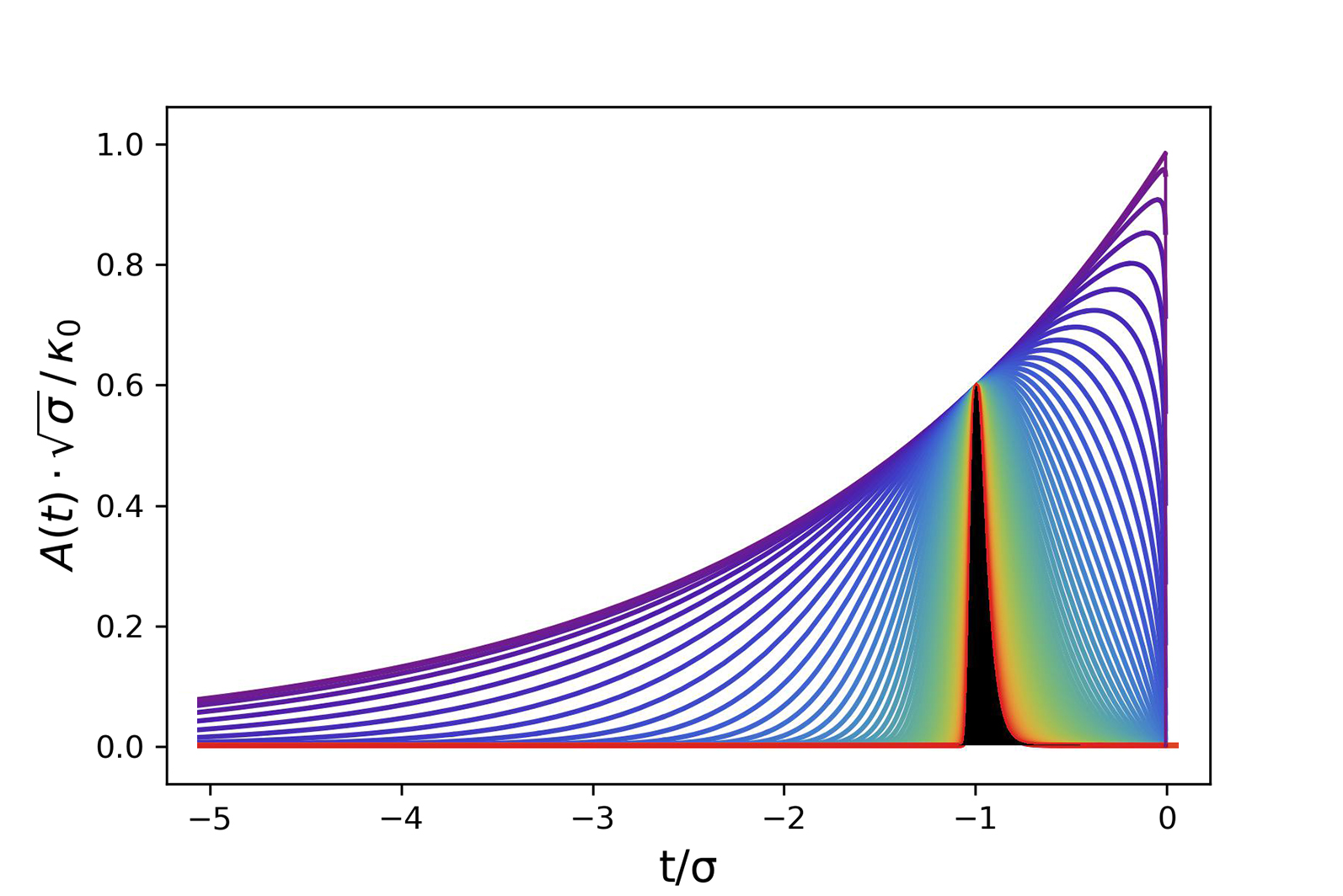
Figure 2.1: The retrodictive probability amplitudes ${A(t)=|\Psi(t)|}$ defined in (2.12) are plotted for polynomial decays of the form ${\kappa(t)=\kappa_{0}\left(\frac{T-t}{\sigma}\right)^{n}}$ with polynomial order $n$ varying from $0$ (violet, top) to $40$ (red, bottom) denoted by color. The polynomial decays correspond to systems where the decay rate drops to zero precisely at the time of detection. Here time is measured with respect to (w.r.t.) time of detection ${T=0}$ and we set ${T_{0}=-\infty}$ so that ${{\cal W}=1}$ (2.13).

Only constant ${\kappa(t)=\kappa_{0}}$ yields non-zero probability amplitude at ${t=0}$ (where it is maximum). This illustrates the two roles $\kappa(t)$ plays: determining the probability $\kappa(t)dt$ with which an excitation can enter the system at a time $t$, and the rate $\kappa(t)$ at which the excited state will decay.This latter effect drives down the probability amplitude for the distant past. For ${\kappa(T)\neq 0}$, the most likely time that a photon entered the system is now (${t=0}$) whereas if ${\kappa(T)=0}$, there is some time of maximum likelihood determined by competition between the two effects (absorption and decay). For no order $n$ are the retrodictive probability distributions continuously differentiable; these simple polynomial couplings do not yield measurements projecting onto smooth wave packets unlike the couplings plotted in Fig. 2.3. Note that $\kappa(t)$ is not normalized and diverges as ${t\rightarrow-\infty}$, yet it results in well-behaved, normalized retrodictive probability amplitudes.

Whereas $f(t)$ is a normalized wavepacket, $\Psi(t)$ is subnormalized for finite $T_{0}$, since

$${\cal W}=\int_{T_{0}}^{T}dt|\Psi(t)|^{2}=1-\exp\left[-\int_{T_{0}}^{T}\!dt\,\kappa(t)\right].$$ (2.13)

We can interpret $\Psi(t)$ as a retrodictive probability amplitude (for simple examples, see Fig. 2.1 and Fig. 2.2), identifying at which times a photon likely entered the system given a detector “click” at $t=T$.

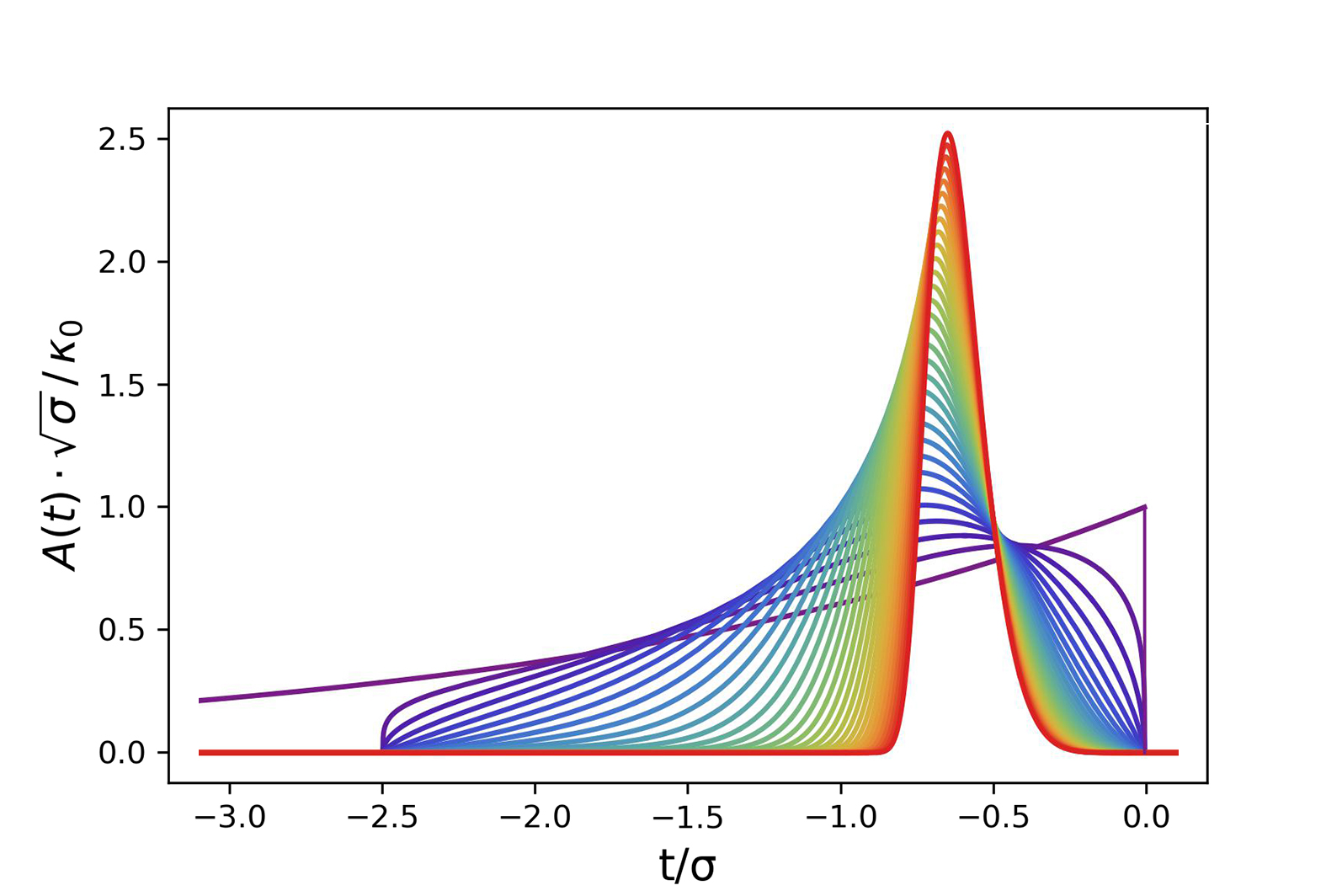
Figure 2.2: Retrodictive probability amplitudes $|\Psi(t)|$ defined in (2.12) are plotted for polynomial decays of the form ${\kappa(t)=\kappa_{0}\left(\frac{t-T_{0}}{\sigma}\right)^{n}\left(\frac{T-t}{\sigma}\right)^{n}}$ for ${T_{0}\leq t\leq T}$, with the polynomial order $n$ varying from $0$ (violet, lowest peak) to $15$ (red, highest peak) denoted by the color. Time is measured w.r.t. detection time ${T=0}$.

Except for ${n=0}$ (also in Fig. 2.1 and included here for reference), these decays become non-zero when the photodetector is turned on at ${T_{0}=-2.5\sigma}$ so that ${\cal W}$ from (2.13) is less than unity. As in Fig. 2.1, for no order $n$ are the retrodictive probability distributions continuously differentiable (indeed, this is the source of the singularity in Ref. [3], and do not project onto smooth wave packets as in Fig. 2.3. Also as in Fig. 2.1, we observe a time of maximum likelihood determined by competition between the two effects (absorption and decay).

We can define a normalized single-photon state

$$\left|\Psi_{T}\right\rangle={\cal W}^{-1/2}\int_{T_{0}}^{T}\!dt\,\Psi(t)\hat{a}^{\dagger}_{\rm in}(t)|{\rm vac}\rangle$$

with the creation operator $\hat{a}^{\dagger}_{\rm in}(t)$ acting on the input continuum of states (it’s Fourier transform $\hat{a}^{\dagger}_{\rm in}(\omega)$ creates a monochromatic state with frequency $\omega$). The arbitrary input single-photon state (which may have been created long before our detector was turned on at $T_{0}$ or long after the measurement ended at time $T$) is

$$\left|f\right\rangle =\int_{-\infty}^{\infty}dtf(t)\hat{a}^{\dagger}_{\rm in}(t)|{\rm vac}\rangle.$$ (2.15)

The commutator relation for the input field operator is $[\hat{a}_{\rm in}(t),\hat{a}^{\dagger}_{\rm in}(t^{\prime})]=\delta(t-t^{\prime})$.

The probability for an arbitrary input photon wavepacket $f(t)$ to result in the system being found in the excited state at a time $T$ is $|C_{1}(T)|^{2}={\cal W}\left\langle f|\Psi_{T}\right\rangle\left\langle\Psi_{T}|f\right\rangle$. The measurement does not project onto times after we have checked if the system is in the excited state, nor onto times before the detector was turned on.

We rewrite this probability in terms of a POVM element containing a single element

$$\hat{\Pi}_{T}={\cal W}\left|\Psi_{T}\right\rangle\left\langle\Psi_{T}\right|$$ (2.16)

To the extent our detector has been open long enough, such that ${\cal W}\rightarrow 1$, our detector could act as a perfectly efficient detector for a specific single-photon wavepacket with temporal mode function $\Psi(t)$. This wavepacket is the time reverse of the wavepacket that would be emitted by our system if it started in the state $\left|1\right\rangle$.

For this simple system, the POVM element is both pure (containing just one term) and (almost) maximally efficient; the weight ${\cal W}$ may approach unity as close as we wish by lengthening the time the detector is on for (that is, taking $T_{0}$ to the distant past and making sure the projected wavepacket [approximately] ends before checking at time $T$).

Here we observe an obvious tradeoff between efficiency and photon counting rate: one cannot project onto a long single-photon wavepacket in a short time interval without cutting off the tails, lowering the overall detection efficiency.

The two-level system described in Eq. (2.7) is a special case but an important one; the two-level system is often a very good approximation of more complicated systems near-resonance. Furthermore, the two-level system is the foundation for generating more complicated network structures, as we will discuss in more detail in the next chapter. In this chapter, we will focus on the simple time-dependent system (2.7) as it is sufficiently general to perform a measurement described by any time-independent system, and more. Indeed, (2.7) is general enough to project onto a completely arbitrary single-photon wavepacket, a result we will now prove.

Proof.— Consider a photon with complex wavepacket $\Psi^{*}(t)=A(t)e^{i\phi(t)}$, positive amplitude $A(t)$, and phase $\phi(t)$. Inserting this into (2.12), we arrive at two separate expressions

$$A(t) = \sqrt{\kappa(t)}e^{-\int_{t}^{T}dt^{\prime}\frac{\kappa(t^{\prime})}{2}}$$

$$\phi(t) = -\int_{t}^{T}dt^{\prime}\Delta(t^{\prime}).$$ (2.19)

The second line is always solvable by $\Delta(t)=\dot{\phi}(t)$ up to a constant global phase shift provided $\phi(t)$ is everywhere differentiable (smooth). We now focus on the first line. Taking the natural logarithm we arrive at an expression

$$2{\rm Ln}[A(t)]-{\rm Ln}[\kappa(t)]=-\int_{t}^{T}dt^{\prime}\kappa(t^{\prime}).$$ (2.20)

Taking the time derivative of both sides, we arrive at a Bernoulli differential equation [125]

$$\kappa^{-2}(t)\frac{d\kappa(t)}{dt}-\frac{2}{A(t)\kappa(t)}\frac{dA(t)}{dt}=-1.$$ (2.21)

Provided $\frac{1}{A(t)}\frac{dA(t)}{dt}$ is continuous, this is solved by

$$\kappa(t)=\frac{A^{2}(t)}{1-\int_{t}^{T}A^{2}(t^{\prime})dt^{\prime}}$$ (2.22)

in agreement with Ref. [119] and Ref. [122]. Here, $\kappa(t)$ is given by the square of the electromagnetic field, divided by a correction factor accounting for the finite response time imposed by $\kappa(t)$ itself. From (2.22), we observe that the only condition imposed on $A(t)$ is that $A^{2}(t)$ has an antiderivative (indefinite integral). We simply require $A^{2}(t)$ be continuous, which in turn requires $A(t)$ to be continuous. Thus, any wavepacket with smooth phase profile $\phi(t)$ and smooth amplitude $A(t)$ is projected onto by some physically realizable single-photon detection scheme. ∎

Special Case: Fourier-Limited Measurement.— A Fourier-limited simultaneous measurement of time and frequency is achieved with a Gaussian time-frequency distribution. We want a temporal wavepacket $\Psi^{*}(t)$ that is the complex square root a Gaussian distribution

$$\Psi^{*}(t)=\frac{1}{(2\pi\sigma^{2})^{\frac{1}{4}}}e^{-\frac{(t-t_{0})^{2}}{4\sigma^{2}}}e^{i\frac{\omega_{0}}{2}t}$$ (2.23)

where $\sigma$ is the temporal half-width, and $t_{0}$ and $\omega_{0}$ are the central time and frequency of the Gaussian distribution. We find that this wavepacket is projected onto by a time-dependent system with constant resonance $\Delta(t)=\omega_{0}$ and a time-dependent coupling

$$\kappa(t)=\frac{e^{-\frac{(t-t_{0})^{2}}{2\sigma^{2}}}}{\sqrt{2\pi\sigma^{2}}(1+\frac{1}{2}{\rm Erf}[\frac{t_{0}-T}{\sqrt{2}\sigma}]-\frac{1}{2}{\rm Erf}[\frac{t_{0}-t}{\sqrt{2}\sigma}])}$$ (2.24)

as in Fig. 2.3. Note that the coupling $\kappa(t)$ is $T$-dependent even though the projected state (2.23) is $T$-independent, in agreement with the general case (2.22).

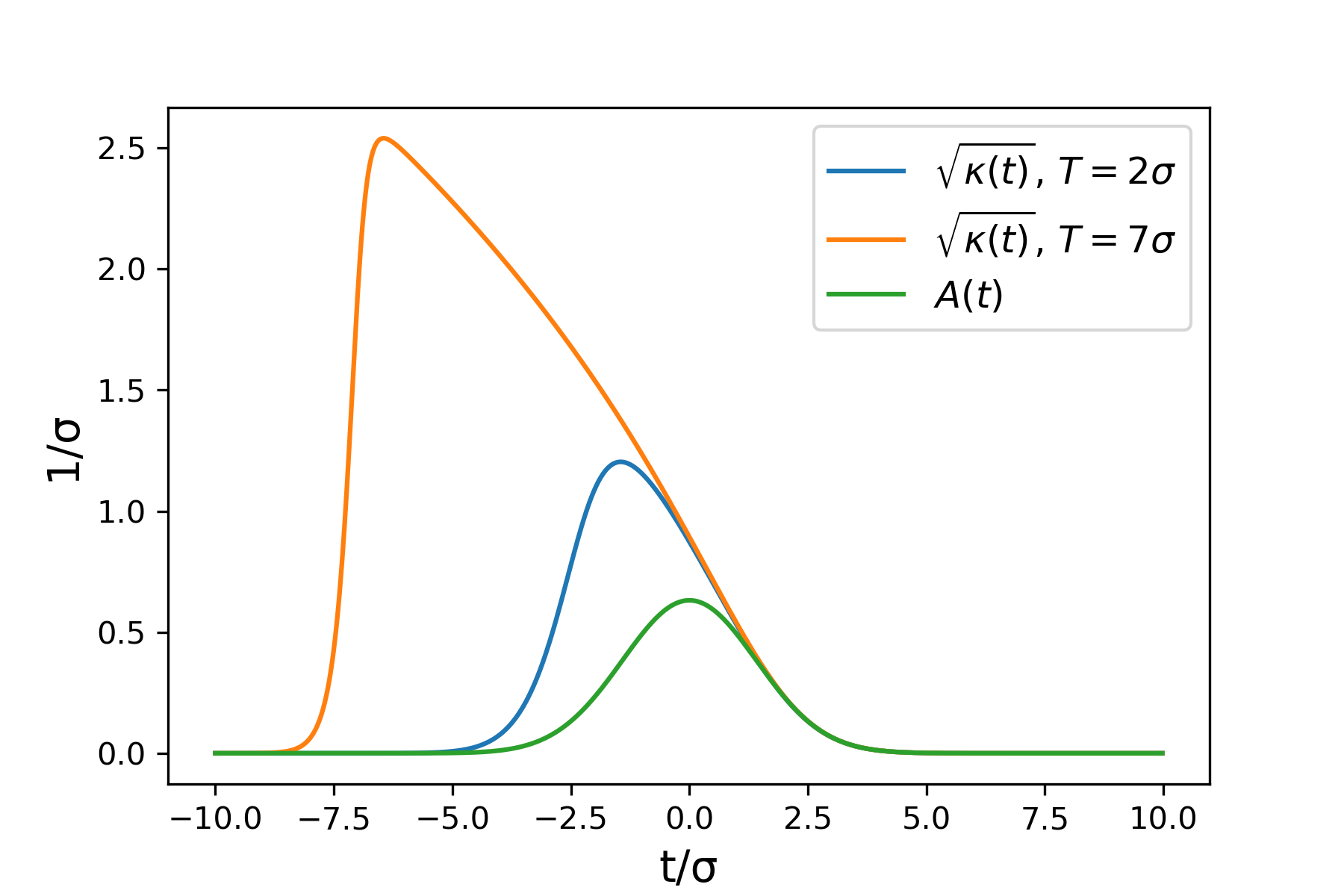
Figure 2.3: Time-dependent couplings $\kappa(t)$ defined in (2.24) generating a minimum uncertainty (Gaussian) wavepacket are plotted for times of detection ${T=2\sigma}$ (${{\cal W}=0.98}$) and ${T=7\sigma}$ (${{\cal W}=1-10^{-10}}$) and detector on-time ${T_{0}=-\infty}$. The retrodictive probability amplitude is now a well-defined wavepacket, with amplitude $A(t)$ depicted in the rotating frame (without fast oscillations at central frequency $\omega_{0}$). Time is measured w.r.t. the wavepacket’s central time $t_{0}$. For times near ${t\approx T}$ the coupling $\sqrt{\kappa(t)}$ is approximately Gaussian as an excitation absorbed at this time will not have sufficient time to decay back out. For earlier times, $\sqrt{\kappa(t)}$ is strictly larger than $A(t)$ and is skewed towards earlier times to incorporate the time it takes the system to respond (${\sim 1/\kappa(t)}$); one needs to prepare the two-level system for the photon, accomplished via a “sharkfin” coupling that precedes the single-photon wavepacket [121]. Near ${t=-T}$, we observe the coupling $\kappa(t)$ rapidly drops to zero, which is a direct consequence of the temporal symmetry of the wavepacket about $t_{0}$. [From (2.12) one can verify that, if $A(t)$ is time-symmetric around ${t=t_{0}}$, the coupling $\kappa(t)$ must satisfy ${\kappa(t_{0}-t)=e^{\int_{t_{0}-t}^{t_{0}+t}dt^{\prime}\kappa(t^{\prime})}\kappa(t_{0}+t)}$.]

2.3 The Three-Stage Model of Photodetection

The model of a SPD as an isolated two-level system is highly idealized. In a more realistic system, photodetection is an extended process wherein a photon is transmitted into the detector, interacting with the system and triggering a macroscopic change of the photodetector state (amplification) which can then be measured classically. Many theories of single-photon detection have been developed over the past century, [44, 47, 48, 49, 126, 50, 51, 127, 52, 26, 24, 25] and indeed there are numerous implementations of SPD technology [128, 129, 22, 66, 23].

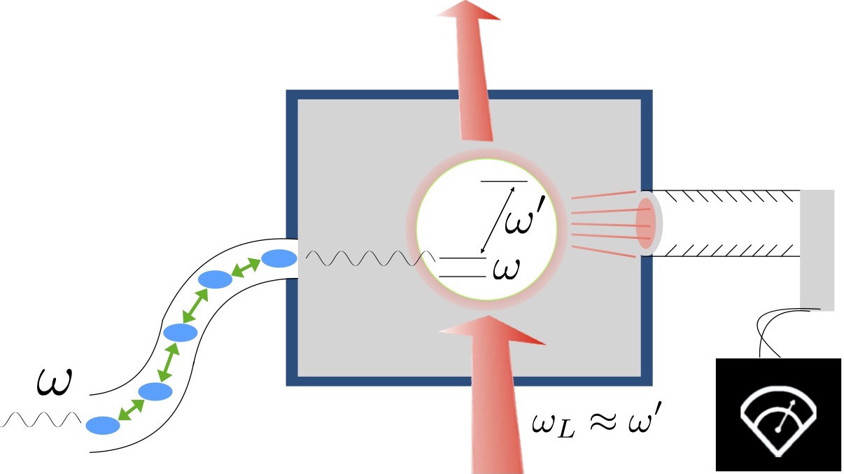
Figure 2.4: The three stages of photodetection in a physical implementation: transmission, amplification, and measurement. An input photon with frequency $\omega$ is transmitted irreversibly via network of coherently coupled discrete states into contact with the photodetection mechanism, here modeled as a two level system. Once the amplification mechanism is triggered by a photon, a macroscopic optical signal with frequency ${\omega^{\prime}\approx\omega_{L}}$ (the laser frequency) is irreversibly created via amplification, in our model implemented with a three-level electron shelving scheme in a single mode cavity; absorption of the single photon at frequency $\omega$ results in many flourescence excitations at frequency $\omega^{\prime}$. This is then converted to a classical electrical readout through a photomultiplier tube (which could have low efficiency) in a third irreversible step. Both initial transmission into the system and absorption by the two-level system filter the light, changing which quantum state is projected onto by the final measurement.

Across all systems, we identify these three stages of transmission, amplification, and measurement as universal in Fig. 2.4. In the next three chapters, we will study the transmission and amplification stages in detail before deriving a POVM that incorporates all three stages quantum mechanically and includes fluctuations of system parameters. The time-dependent two-level system from the previous section enabling arbitrary wavepacket projection will be incorporated into the three-stage model as the trigger for the amplification mechanism. We will assume in this analysis that the system is left on for a sufficient time such that the subnormalization of $\Psi(t)$ is minimal and ${\cal W}\approx 1$ (2.13).

Chapter 3 Transmission

We now study in detail the topic of the “transmission” stage of photo detection, wherein a photonic signal is transmitted into the photodetector, potentially changing form (transduction) and being absorbed by the device. To accomplish this, the photon has to interact with one or more charged particles, its excitation energy will be converted into other forms of energy which will (in the next stage) lead to a macroscopic signal (amplification), and then a “click” (measurement). A simple example of this is a fiber optical cable: here, a discrete fiber mode acts as intermediary between two continua. More complicated forms of energy transport are also described by quantum networks of coupled coupled discrete quantum states and structured continua (e.g. band gaps) provide generic models for that first part of the detection process, as we will discuss in this chapter. The input to the network is a single continuum (the continuum of single-photon states), the output is again a single continuum describing the next (irreversible) step. The process of a single photon entering the network, its energy propagating through that network, and finally exiting into another output continuum of modes can be described by a single dimensionless complex transmission amplitude, $T(\omega)$. Along with $T(\omega)$, we calculate a complex reflection amplitude $R(\omega)$ which characterizes light reflected off of the photodetector. In this chapter, we discuss how to obtain from $T(\omega)$ the photo detection efficiency, how to find sets of parameters that maximize this efficiency, as well as expressions for other input-independent quantities such as the frequency-dependent group delay and spectral bandwidth of the transmission portion of a single-photon detector. We then study a variety of networks, discuss how to engineer different transmission functions $T(\omega)$ amenable to photo detection, and discuss implications for single-photon detection technology.

The underlying basics of photodetection theory was developed in the early 1960s [130, 55, 47], with the quantum nature of light being taken into account, and with later additions to the theory also incorporating the backaction of the detector on the detected quantum field [48, 49, 50, 51, 52]. More recent additions to the theory have analyzed more deeply the amplification process by itself [5] and its relation to the absorption and transduction part of the process [26, 127]. In particular, it turns out that for an ideal detector one should decouple the two processes, by having an irreversible step in between the two, such that the amplification part does not interfere negatively with the absorption (and possibly, transduction) stage, here called transmission [26, 52]. This decoupling will be assumed in this analysis, too.

In order to develop a useful fully quantum-mechanical theory we cannot be completely general; or, rather, if we are completely general, then the only statements on fundamental limits we can make are likely going to be merely examples of Heisenberg’s uncertainty relations. So we will make three restrictive but—we think—reasonable assumptions about our quantum theory of photo detection.

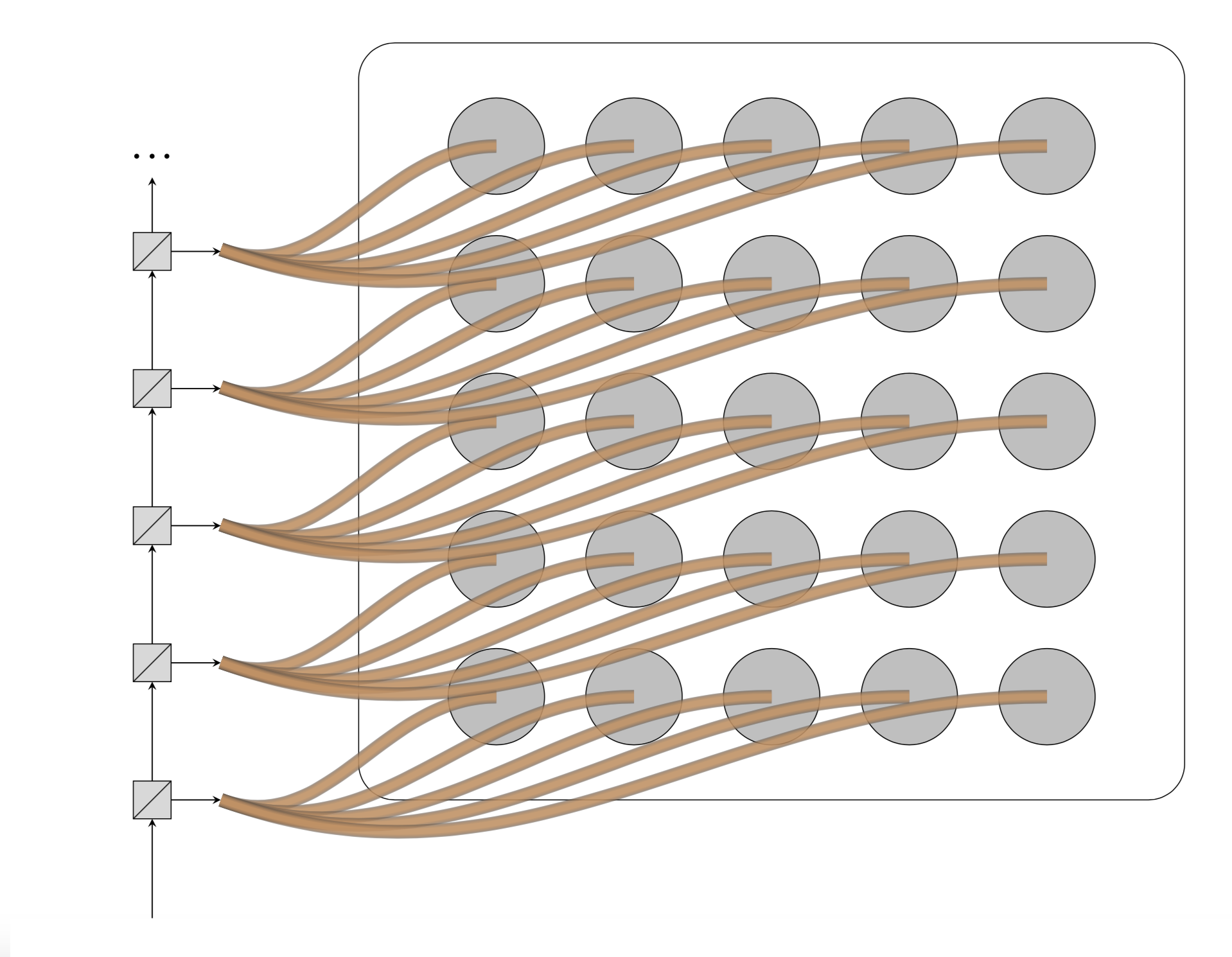
Figure 3.1: An array of single-photon detecting (SPD) pixels. A series of beamsplitters with low reflectivity ensure that at most one photon is incident on each single-photon detector.

First, we focus on single-photon detection. The main reason is that number-resolved photo detection is possible using arrays of SPDs where each “pixel” receives at most one photon as in Fig. 3.1 (also see [131, 132], or [133] for the time-reversed process of creating a single photon on demand). So we focus on an individual pixel here. (See Ref. [134] for a modeling framework for systems with multiple inputs and Refs. [135, 136, 137] for non-linear S-matrix treatments of few-photon transport.)

Second, although a general state of a single photon is a function of four quantum numbers, one related to the spectral degree of freedom, two related to the two transverse spatial degrees of freedom, and one related to the polarization or helicity degree of freedom, we will restrict ourselves to the spectral (or, in the Fourier transformed-picture, the temporal) degree of freedom. That is, the input state can be defined in terms of frequency-dependent creation operators $\hat{a}^{\dagger}(\omega)$ acting on the vacuum. The reason is that the other three degrees of freedom can, in principle, if not in practice, be sorted before detection. For example, if one wishes to distinguish between horizontally and vertically polarized photons, one may use a polarizing beam splitter and put two detectors behind each of the two output ports. Similarly, efficient sorting of photons by their orbital angular momentum quantum number [104] and spatial mode are also possible [105, 106]. It is easier to consider sorting as part of the pre-detection process, rather than a task for the detector itself . On the other hand, the spectral response of a detector cannot be eliminated; the time-frequency degree of freedom is intrinsic to the resonance-structure of the photo detecting device.

Third, we are going to assume that the transmission stage of each pixel’s operation is passive. That is, apart from being turned on at some point, and being turned off at some later point, it operates in a time-independent manner with time-independent decay rates, couplings, and resonance structure. Thus, an incoming photon will interact with a time-independent quantum system. As we will see, active filtering is not needed for perfect detection provided the photodetector has no internal losses (couplings to additional continua or side channels). Furthermore, including a time-dependent amplification trigger allows for arbitrary wavepacket detection, a result we will show in Chapter V.

We can now describe the interaction of a single photon with an arbitrary quantum system as follows. The system may be naturally decomposed into subsystems, each of which may have discrete and/or continuous energy eigenstates. (For example, the photon may be absorbed by a molecule or atom or quantum dot or any structure with a discrete transition that is almost resonant with the incoming photon.) The continua will in general be structured (for example, containing bands and band gaps in between) [138, 139, 140], but structured continua can be equivalently described as structureless (flat) continua coupled to (fictitious) discrete states [109, 110, 111, 89], enabling a Markovian description of the system independent of an input photon’s bandwidth. Indeed, it is well known that a non-Markovian open system can always be made Markovian by expanding the Hilbert space (the converse of the Stinespring dilation [141]). And so an arbitrary quantum system may be described by a network of discrete states (some physical, some fictitious), coupled to flat continua. The latter coupling makes the time evolution irreversible. Of course, an actual detector is indeed irreversible. In particular, the amplification process (converting the microscopic input signal into a classical macroscopic output signal) is intrinsically irreversible.

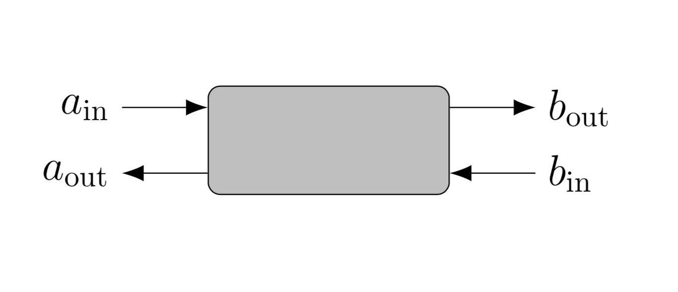
Figure 3.2: Input and output fields coupled to a two-port black box quantum network. The input and output operators are continuous mode (as functions of frequency $\omega$) annihilation operators, satisfying canonical commutation relations [4]. Here the mode $a_{{\rm in}}(\omega)$ carries the single-photon input state, the reflected mode is described by $a_{{\rm out}}(\omega)$, and the output mode $b_{{\rm out}}(\omega)$ contains the excitation energy if the input energy successfully traversed the network (and may serve as input to the next part of the photo detection process, e.g., amplification, see Ref. [5]). $b_{{\rm in}}(\omega)$ may contain thermal excitations, but is never occupied by the photon we wish to detect.

As we will show, this first part of the process can then be fully described in terms of a complex transmission amplitude $T(\omega)$, which is the probability amplitude for the component of the input signal at frequency $\omega$ to enter the next (amplification) process. (By then the energy $\hbar\omega$ will have been converted into a different type of energy, i.e., a different type of excitation, but that plays no particular role here.) It is straightforward to calculate the transmission function through a network (the equations are linear!). The point here is that from $T(\omega)$ we can determine three input-independent quantities of interest to the photo detection process. (That one complex function $T(\omega)$ is sufficient is due to our considering only the time/frequency degree of freedom.)

This chapter is organized as follows. After defining our quantities of interest in section II (short), we start with analyzing the simplest quantum network to illustrate how we calculate $T(\omega)$ and how our three quantities of interest behave in section III (also short). We then present a systematic survey of more complicated networks in the much longer section IV; for each network class, we analytically calculate $T(\omega)$ and discuss the behavior of the three quantities of interest. Then in section V, we briefly discuss extensions to arbitrary quantum networks including the effects of couplings to additional continua/side channels before summarizing our findings in the conclusions.

3.1 Quantities of Interest

Here, we define three quantities of interest derivable from $T(\omega)$, and discuss their applicability to photo detecting systems.

First, $|T(\omega)|^{2}$ itself gives an upper bound on the probability for the frequency component $\omega$ to be detected. (If there were no losses downstream in the photodetection process, it would equal the probability of detection of monochromatic light at that frequency.) We are thus particularly interested in identifying quantum systems for which there is at least one frequency $\omega_{i}$ for which $|T(\omega_{i})|=1$.

Second, an upper bound to the total detectable frequency range of input light is given by the spectral bandwidth of the quantum network (not to be confused with the channel bandwidth in [98] or the range of a single frequency band [142]). We define this quantity

$$\tilde{\Gamma}=\frac{1}{\pi}\int_{0}^{\infty}d\omega|T(\omega)|^{2}.$$ (3.1)

(The $\frac{1}{\pi}$ factor gives agreement with a classical Lorentzian filter; the transmission function is $T(\omega)=\frac{\Gamma}{\Gamma-i(\omega-\omega_{0})}$ for a filter with damping factor $\Gamma$ and resonant frequency $\omega_{0}$ and we find $\tilde{\Gamma}=\Gamma$, see Eq. (3.14) below.) The inverse of this quantity is also a measure of the time the photon spends in the detector. (Indeed, $\tilde{\Gamma}^{-1}$ is a lower bound on timing jitter from integrated detection event when quasi-monochromatic photon states are detected with high efficiency, see footnote.)

Third, we can also define a delay (latency) using the polar decomposition of $T(\omega)$

$$T(\omega)=|T(\omega)|\exp(i\phi(\omega))$$ (3.2)

and using the standard definition of group delay as

$$\tau_{g}(\omega)=-\frac{d\phi(\omega)}{d\omega}.$$ (3.3)

We can see how this group delay directly relates to an experimentally-measured latency by considering a temporal wavepacket $\psi_{\rm in}(t)$ and Fourier transform $\tilde{\psi}_{\rm in}(\omega)$. We can then write the output single-photon state

$$\left|\psi^{\prime}\right\rangle = \int_{0}^{\infty}d\omega\tilde{\psi}_{\rm in}(\omega)R(\omega)\hat{a}^{\dagger}_{\rm out}(\omega)|{\rm vac}\rangle$$ (3.4)

$$+ \int_{0}^{\infty}d\omega\tilde{\psi}_{\rm in}(\omega)T(\omega)\hat{b}^{\dagger}_{\rm out}(\omega)|{\rm vac}\rangle$$

where the first and second terms correspond to the reflected and transmitted parts of the single-photon state, respectively (for details, see Ref. [143]) and we have introduced a reflection coefficient $R(\omega)$ satisfying $|T(\omega)|^{2}+|R(\omega)|^{2}=1$ and $R^{*}(\omega)T(\omega)+R(\omega)T^{*}(\omega)=0$ at every frequency $\omega$. From (3.4) we note that, after interacting with the network, the transmitted wavepacket will have the form $\psi_{\rm out,T}(t)=FT^{-1}[\tilde{\psi}_{\rm in}(\omega)T(\omega)]$. (Note that the wavepacket described by $\psi_{\rm out,T}(t)$ will be sub-normalized by construction; it only corresponds to the portion of the full single photon state $\psi^{\prime}(t)\equiv\left\langle t|\psi^{\prime}\right\rangle$ that is transmitted!) For a long input pulse with central frequency $\omega^{\prime}$, we find $\psi_{\rm out,T}(t)\approx|T(\omega^{\prime})|\psi_{\rm in}(t-\tau)e^{i\omega^{\prime}\tau^{\prime}}$ with $\tau^{\prime}$ the difference between the group delay $\tau_{g}(\omega^{\prime})$ defined above and the (here irrelevant) phase delay.

The effect of the group delay on an arbitrary input photon state is to selectively delay and reshape the transmitted wavepacket. Of course, if an input photon has a wide spread of frequencies, a differential group delay $\tau_{g}(\omega)=-\frac{d\phi(\omega)}{d\omega}$ may increase (or decrease) the temporal spread of the wavepacket, as it will affect each frequency differently. This increase (or decrease) in the arrival times of different frequencies is manifestly input-dependent and will not play a role in the input-independent temporal uncertainty or jitter. We can, however, define an additional quantity characterizing the input-independent group delay-induced dispersion

$$\mathcal{T}_{g}=\int_{0}^{\infty}d\omega\left|\frac{d\tau_{g}(\omega)}{d\omega}\right||T(\omega)|^{2}$$ (3.5)

whose definition agrees with our physical intuition that a constant group delay over the transmission window will not contribute to dispersion, nor will frequencies that are not transmitted regardless of how large $\frac{d\tau_{g}(\omega)}{d\omega}$ may be. We find that, for a flat transmission function that is unity over some spectral range $\omega_{0}\pm\delta\omega$ and zero everywhere else and a monotonic group delay $\tau_{g}(\omega)$, (3.5) gives the difference in group delay between the minimum and maximumly transmitted frequencies: $\mathcal{T}_{g}=|\tau_{g}(\omega_{0}-\delta\omega)-\tau_{g}(\omega_{0}+\delta\omega)|$. This is the maximum dispersion possible for any input to this system.

Finding key conditions that change the transmission function $T(\omega)$ and frequency-dependent group delay $\tau_{g}(\omega)$ are important for the design of coupled-resonator optical waveguide (CROW) networks [144] for delay-lines [145] and spectral filtering [146], where the transmission efficiency, frequency-dependent group delay, and spectral bandwidth will all affect performance. These are the three quantities we focus on in the rest of the chapter.

Knowing $T(\omega)$ for a specific photodetector also allows one to construct a simplified positive-operator valued measure (POVM) by assuming any excitation in the output continuum results in a click (for details, see the last section of this chapter). The simple POVM element corresponding to a click after the photodetector has been left on for a very long time (in particular, long compared to the bandwidth $\tau\gg\tilde{\Gamma}^{-1}$) has the particularly simple form

$$\hat{\Pi}=\int_{0}^{\infty}\,d\omega\,|T(\omega)|^{2}\left|\omega\right\rangle\left\langle\omega\right|.$$ (3.6)

$\hat{\Pi}$ is defined such that the probability of a photon in an arbitrary input state $\hat{\rho}$ being detected is given by the Born rule $\textnormal{Pr}=\textnormal{Tr}\left(\hat{\Pi}\hat{\rho}\right)$. For example, any photon state $\hat{\rho}=\sum_{i}\lambda_{i}\,\left|\omega_{i}^{\prime}\right\rangle\left\langle\omega_{i}^{\prime}\right|$ where $|T(\omega_{i}^{\prime})|^{2}=1$ and $\sum_{i}\lambda_{i}=1$ will be detected with unit probability. (The states the photodetector can detect perfectly include both pure states [when only one $\lambda_{i}$ is non-zero] and mixed states comprised entirely of frequencies where $|T(\omega_{i}^{\prime})|^{2}=1$.) Of course, no photon is truly monochromatic (or discretely polychromatic), but it can be effectively so if the wave-packet envelope is long compared to the inverse spectral bandwidth $\tilde{\Gamma}^{-1}$.

3.2 Simple example

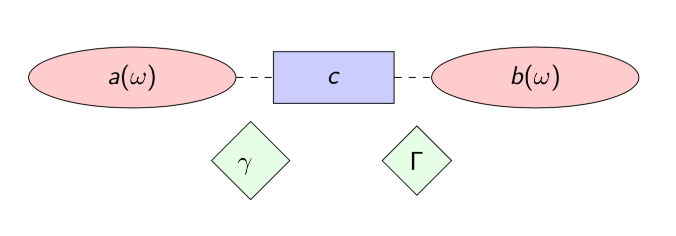
Figure 3.3: A simple network comprised of a single discrete state described by an operator $c$ (the bosonic replacement for the two-level system fermionic lowering operator $\sigma^{-}$) and decaying to left (input, external) and right (output, internal) continua $a$ and $b$ at rates $\gamma$ and $\Gamma$, respectively. That is, here the black box of Fig. 3.2 contains just one two-level system. This exactly describes filtering of light by a Fabry-Perot cavity.

The simplest quantum network consists of a single two-level system with a ground state $\left|g\right\rangle$ and an excited state $\left|e\right\rangle$, with the incoming photon coupling these states (Fig. 3.3). The two-level system is described by fermionic raising and lowering operators $\sigma^{+}=\left|e\right\rangle\left\langle g\right|$ and $\sigma^{-}=\left|g\right\rangle\left\langle e\right|$ (this is also the simplest model of a photodetector, see [130]). Physically, this excited state could be any discrete state of a single absorber, e.g. the p-state of an atom (that is, an atomic excited state with exactly one quanta of angular momentum) which then decays to a monitored flat continuum. (Indeed, single absorbers such as atoms [147, 148, 149, 150, 151, 77], single molecules [152], NV-centers [153], and quantum emitters [154, 155] are able to efficiently couple to and absorb single photons.)

In the Heisenberg picture, the evolution of these raising and lowering operators $\sigma^{+}$ and $\sigma^{-}$ will determine whether a photon makes it from one side of the network to the other. By focusing our analysis on cases where at most a single photon is in the network, we can use the equivalence between the two-level system and the simple harmonic oscillator to simplify our problem ab initio: we replace the fermionic raising and lowering operators with bosonic creation and annihilation operators $c^{\dagger}$ and $c$.

We follow standard input-output theory here [4], separating the full evolution of both continua $a$ and $b$ into input and output modes (Fig. 3.2). By formally solving the Heisenberg evolution equations for the two input continuum mode annihilation operators $b_{{\rm in}}$ and $a_{{\rm in}}$, we can write the effective system Hamiltonian that governs the evolution of the system operators $c$ and $c^{\dagger}$

(3.7)

$$H =\hbar\omega_{0}c^{\dagger}c-\sqrt{\gamma}(c^{\dagger}a_{{\rm in}}+ca^{\dagger}_{{\rm in}})-\sqrt{\Gamma}(c^{\dagger}b_{{\rm in}}+cb^{\dagger}_{{\rm in}})$$

where we have identified $\omega_{0}$ as the resonance frequency, and $\gamma$ and $\Gamma$ as the left and right side couplings to two continua $a$ and $b$ respectively. In the Heisenberg picture, the time evolution of the discrete state annihilation operator is given by

$$\dot{c}=-i\omega_{0}c-\frac{\gamma+\Gamma}{2}c-\sqrt{\gamma}a_{{\rm in}}-\sqrt{\Gamma}b_{{\rm in}}.$$ (3.8)

The input mode operators $a_{{\rm in}}$ and $b_{{\rm in}}$ and output mode operators $a_{{\rm out}}$ and $b_{{\rm out}}$ are determined by open quantum system evolution of the discrete state operator $c$ in (3.8) and the two boundary conditions

$$a_{{\rm out}}-a_{{\rm in}}=-\sqrt{\gamma}c$$

$$b_{{\rm out}}-b_{{\rm in}}=-\sqrt{\Gamma}c.$$ (3.9)

It is easiest to solve the equations by taking the Fourier transform. Unitarity implies the existence of a transfer matrix relating in and out fields in the spectral domain

$$\begin{bmatrix}a_{{\rm out}}(\omega)\\ b_{{\rm out}}(\omega)\\ \end{bmatrix}=\begin{bmatrix}R(\omega)&T(\omega)\\ T(\omega)&R(\omega)\\ \end{bmatrix}\,\begin{bmatrix}a_{{\rm in}}(\omega)\\ b_{{\rm in}}(\omega)\\ \end{bmatrix}$$ (3.10)

where $|T(\omega)|^{2}+|R(\omega)|^{2}=1$ (resulting from our assumption there are no internal losses) [157]. Defining a detuning $\Delta=\omega-\omega_{0}$, we can easily solve (3.8) in terms of the Fourier transform of the discrete state annihilation operator

$$c(\omega)=\frac{-\sqrt{\gamma}a_{{\rm in}}(\omega)-\sqrt{\Gamma}b_{{\rm in}}(\omega)}{\frac{\gamma+\Gamma}{2}-i\Delta}$$ (3.11)

yielding a transmission function

$$T(\omega)=\frac{\sqrt{\gamma\Gamma}}{\frac{\gamma+\Gamma}{2}-i\Delta}.$$ (3.12)

We can see from (3.13) that perfect transmission ($|T(\omega)|^{2}=1$) occurs only when $\gamma=\Gamma$ and $\Delta=0$. These are the well-known conditions of balanced mirrors and on-resonance required for perfect transmission through a Fabry-Perot cavity [124].

We can also calculate the frequency dependent group delay

$$\tau_{g}(\omega)=\frac{\frac{\Gamma+\gamma}{2}}{\left(\frac{\Gamma+\gamma}{2}\right)^{2}+\Delta^{2}}.$$ (3.13)

Like $T(\omega)$, the group delay is also a Lorentzian with width $\frac{\Gamma+\gamma}{2}$, and that frequencies close to resonance spend the most time in the network with a maximum group delay of $\frac{2}{\Gamma+\gamma}$ on resonance. We similarly find the input-independent group delay-induced dispersion (3.5) to be $\mathcal{T}_{g}=\frac{8\gamma\Gamma}{(\gamma+\Gamma)^{3}}$.

We can also use $T(\omega)$ to calculate a spectral bandwidth (not to be confused with the channel bandwidth discussed in [98])

$$\tilde{\Gamma} =\frac{1}{\pi}\int_{0}^{\infty}\,d\omega\,|T(\omega)|^{2}$$ (3.14)

$$=\frac{2\Gamma\gamma}{\Gamma+\gamma}$$

which is a measure of the number of frequencies that can be efficiently detected. For this simple case, we note that $\tau_{g}(\omega)=\tilde{\Gamma}^{-1}|T(\omega)|^{2}$ and thus $\int\,d\omega\tau_{g}(\omega)=\pi$. While this expression will not be true for a general network, the shift in phase by $\pi$ as a resonance frequency is crossed is a universal feature of networks, as we shall see shortly

3.3 Quantum Networks

We now set up the general problem of an arbitrary network of discrete states connecting two continua. The Hamiltonian is a straightforward generalization of (3.7)

$$\hfill H=\sum_{i}\hbar\omega_{i}c^{\dagger}_{i}c_{i} - \sum_{ij}g_{ij}(c_{i}c^{\dagger}_{j}+c^{\dagger}_{i}c_{j})\hfill\phantom{211}$$ (3.15)

$$-\sum_{i}\sqrt{\gamma_{i}}(c^{\dagger}_{i}a_{{\rm in}}+c_{i}a^{\dagger}_{{\rm in}}) - \sum_{i}\sqrt{\Gamma_{i}}(c^{\dagger}_{i}b_{{\rm in}}+c_{i}b^{\dagger}_{{\rm in}})$$

where we’ve now defined a real coherent coupling between discrete states $g_{ij}$ (we define $g_{ii}=0$ for each state). Some states may not be coupled to one (or both) continuum, in which case either $\sqrt{\gamma_{i}}$ or $\sqrt{\Gamma_{i}}$ (or both) will be zero.

We can similarly generalize the operator evolution in (3.8) for an arbitrary network; moving to the spectral domain, we write the spectral dependence of the discrete state operators

$$-i\Delta_{i}c_{i}(\omega)= -\sum\limits_{j}\,\left(\frac{\sqrt{\gamma_{i}\,\gamma_{j}}+\sqrt{\Gamma_{i}\,\Gamma_{j}}}{2}+ig_{i\,j}\right)c_{j}(\omega)-\sqrt{\gamma_{i}}\,a_{\rm in}(\omega)-\sqrt{\Gamma_{i}}\,b_{\rm in}(\omega).$$ (3.16)

Similarly to (3.2), we can write boundary conditions for the two continua with an arbitrary network

$$a_{{\rm out}}(\omega)-a_{{\rm in}}(\omega)=-\sum\limits_{i}\sqrt{\gamma_{i}}c_{i}(\omega)$$

$$b_{{\rm out}}(\omega)-b_{{\rm in}}(\omega)=-\sum\limits_{i}\sqrt{\Gamma_{i}}c_{i}(\omega).$$ (3.17)

To move from (3.3) to the transfer matrix (4.28) involves solving $N$ systems of $N$ coupled first-order differential equations, as each discrete state amplitude $c_{i}(\omega)$ depends on every other amplitude. Three methods for solving these equations are as follows.

The first is to take the weak-coupling limit $2\,g_{ij}\ll\sqrt{\gamma_{i}\,\gamma_{j}}+\sqrt{\Gamma_{i}\,\Gamma_{j}}\,\forall i,j$ and truncate the solutions after some power in $g_{ij}$, making (3.19) the $0$th order approximate solution with higher order corrections. However, this method fails if even a single discrete state decouples from both continua, as is the case for many networks of interest.

The second is to use numerical techniques to diagonalize the systems of equations and find the transmission function numerically [158]. However, this rapidly gets harder with large systems, and masks the analytic conditions for perfect transmission we are interested in identifying.

The third method is to use a variety of mathematical techniques to solve these $N$ systems of $N$ coupled first-order differential equations analytically, which is the route taken in this analysis. These tricks include making use of correlations between discrete states, permuting labels, and using generalized continued fraction formulae. Here, we will use these techniques to describe three large classes of systems that can be solved exactly with arbitrary couplings, decays, and resonant frequencies. These are parallel networks, series networks, and hybrid networks.

Parallel: each discrete state is directly coupled to both continua ($\gamma_{i}\neq 0$ and $\Gamma_{i}\neq 0\,\forall i$) but not to each other. Thus there are multiple parallel paths to the same final state and hence we’ll get interference. Physical photo detection platforms described by parallel networks include (i) single atoms with multiple p-states that then decay directly to a continuum (similarly for trapped ions/atoms due to Stark and Zeeman effects, see Ref. [159] for this in generating single photons), (ii) quantum dots [160], (iii) structured continua with multiple pseudomodes [161].

Series: each of the two continua are coupled to their own discrete state, which are in turn coherently coupled by a chain of intermediate single discrete states. There is just one path from the input continuum to the output continuum. This model describes (i) an atom in a p-state that first decays to a d-state or metastable s-state before decaying to a flat continuum (and analogously for a molecule [26]), (ii) coherently coupled frequency filtering in front of a photo detecting platform (for instance, using an antireflective coating [20] or optical cavities [162]), (iii) atomic chains coupled through their p-states (which could be mediated by, for example, a fiber mode [163]).

Hybrid: a combination of the above cases. For example, two parallel paths of three steps each or, more generally, layered structured continua (a photon must pass through one before the other). A physical system that can be modeled with a hybrid network is a photosynthetic light-harvesting (i.e. Fenna–Matthews–Olson) complex with multiple paths for coherent transport [164, 165, 166].

In all cases, we will solve the systems of equations for $R(\omega)$ directly and make use of the identities $|T(\omega)|^{2}=1-|R(\omega)|^{2}$ and $T^{2}(\omega)=-R^{2}(\omega)\frac{|T(\omega)|^{2}}{|R(\omega)|^{2}}$when we calculate the transmission efficiency, spectral bandwidth, and group delay.

3.3.1 Parallel Networks

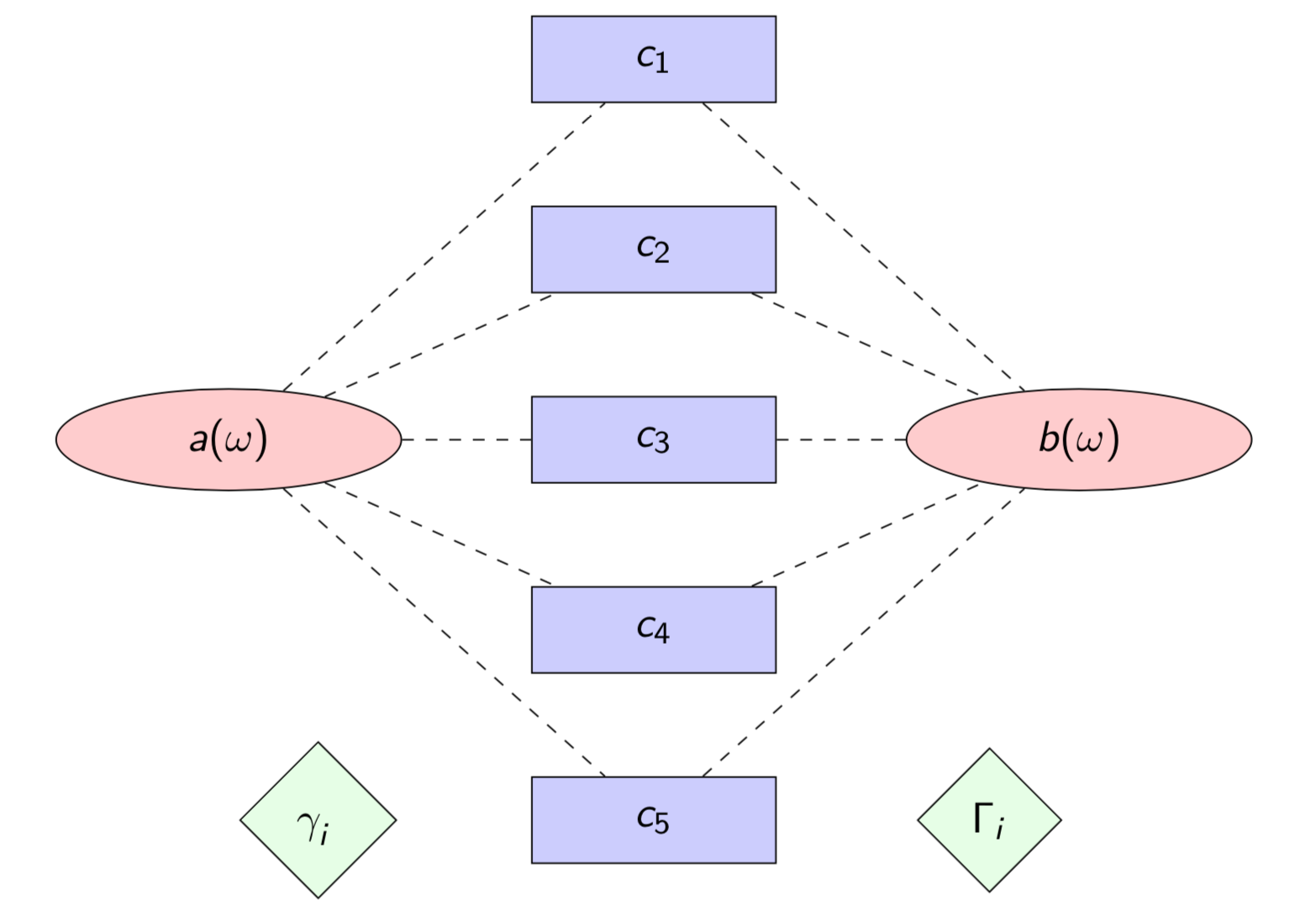
Figure 3.4: A parallel network of ${N=5}$ decoupled discrete states, each described by an operator $c_{i}$ and decaying to left (input, external) and right (output, internal) continua $a$ and $b$ at rates $\gamma_{i}$ and $\Gamma_{i}$, respectively.

We now consider a parallel quantum network where each discrete state is directly coupled to both continua (Fig. 3.4). If the discrete states are directly coupled to each other, it is helpful to first diagonalize the system in the basis where they are decoupled. We then consider the new modes to be the discrete states a photon can occupy, each with a new resonance frequency and two decay rates to the two continua. (In the strong coupling limit, Rabi splitting comes into effect and these dressed states are the more physical description anyways [45].) This decoupled manifold of discrete states, each decaying at a rate $\gamma_{i}$ to the input continuum and a rate $\Gamma_{i}$ to the output continuum (Fig. 3.4), is the next simplest case to analyze, and provides a simple model of a photodetector with a simple band structure.

We find the frequency dependence of the discrete state operators

$$-i\Delta_{i}c_{i}(\omega)= -\sum\limits_{j}\,\frac{\sqrt{\gamma_{i}\,\gamma_{j}}+\sqrt{\Gamma_{i}\,\Gamma_{j}}}{2}c_{j}(\omega)$$ (3.18)

$$-\sqrt{\gamma_{i}}\,a_{\rm in}(\omega)-\sqrt{\Gamma_{i}}\,b_{\rm in}(\omega).$$

A salient feature of Eq. 3.18 is the decay terms produce purely virtual coupling between discrete states coupled to the same continua. These cannot be thought of as coupling mediated by continua, as the continua are flat (Markovian) and perfectly dissipative. If an excitation exits the discrete states and enters a continuum, there is no possibility of its ever returning to another discrete; energy transfer from one discrete state is impossible! Thus, the coupling is purely virtual, and we must instead consider it to be a purely information-theoretic phenomena.

We use (4.28) to find $R(\omega)$ by considering an input on only one side of the network (thus setting the expectation value of the other input field operator to zero). This yields an expression $a_{out}(\omega)=R(\omega)a_{in}(\omega)$ (or $b_{out}(\omega)=R(\omega)b_{in}(\omega)$), from which we reconstruct $T(\omega)$. We analytically find the general form of $R(\omega)$

$$R(\omega)=\frac{\prod\limits_{i}\left(\frac{\Gamma_{i}-\gamma_{i}}{2}-i\Delta_{i}\right)-X_{-}^{(N)}}{\prod\limits_{i}\left(\frac{\Gamma_{i}+\gamma_{i}}{2}-i\Delta_{i}\right)-X_{+}^{(N)}}$$ (3.19)

where $X_{\pm}^{(N)}$ is a polynomial of order $N-2$ in the detunings $\Delta_{i}$. (We find $X_{\pm}^{(1)}=0$.) For $N=2$, we can see that $X_{\pm}^{(2)}$ is symmetric (anti-symmetric) between $\Gamma_{i}$ and $\gamma_{i}$

$$X_{\pm}^{(2)}=\left(\frac{\sqrt{\Gamma_{1}\Gamma_{2}}\pm\sqrt{\gamma_{1}\gamma_{2}}}{2}\right)^{2}.$$ (3.20)

This (anti-)symmetry is also present in higher-$N$ coefficients. From (3.19) we can determine a key feature of parallel quantum networks: if some subset of the discrete states have balanced decay rates such that $\gamma_{i}=\Gamma_{i}$, for large spacings between discrete states compared to the other decay rates $|\omega_{i}-\omega_{j}|\gg\gamma_{j},\Gamma_{j}$, we find $R(\omega_{i})=0$; input monochromatic photons with frequencies on resonance with those discrete states are transmitted perfectly through the network.

In general, finding the specific form of $X_{\pm}^{N}$ is a numerical task, and we will focus on a simpler case where we can utilize another salient feature of parallel networks: the purely virtual coupling present in (3.18). Before we consider a network that is uniformly coupled (all decays are the same), we can consider a network with couplings that are inhomogeneous but uniformly unbalanced such that $\Gamma_{i}=k\,\gamma_{i}\,\forall i$. We can then write (3.18) in a simplified form

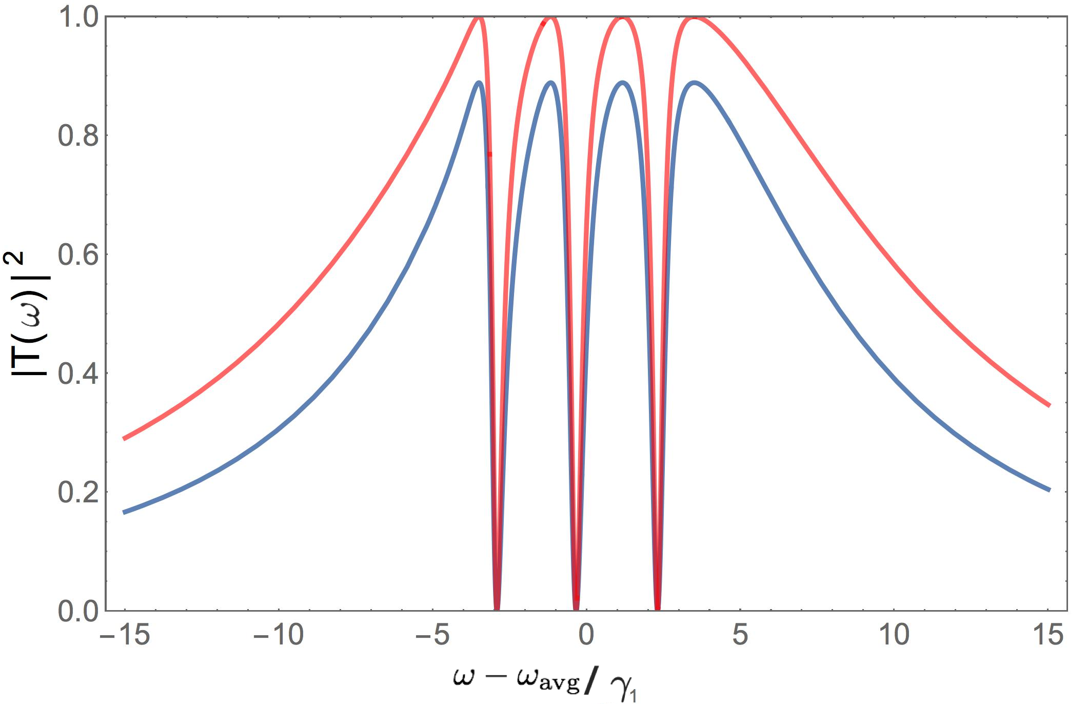
Figure 3.5: Transmission probability for parallel networks with ${N=4}$ equally spaced discrete states, each with a decay rate to the input continuum ${\gamma_{i}=\gamma_{1}\,(\frac{7}{5})^{i-1}}$. The decays to the monitored output continuum are uniformly unbalanced (${\frac{\Gamma_{i}}{\gamma_{i}}=k\,\forall i}$), with ${k=\frac{1}{2}}$ for the blue (lower) curve and ${k=1}$ for the red (upper) curve. Frequency is measured w.r.t. the average resonance frequency. The four resonance frequencies $\omega_{i}$ have maximum transmission probability ${|T(\omega_{i})|^{2}=\frac{4k}{(k+1)^{2}}}$. The three frequencies of perfect reflection (i.e, ${T(\omega_{i})=0}$) correspond to solutions of ${\sum_{i}\frac{\gamma_{i}}{\Delta_{i}}=0}$.

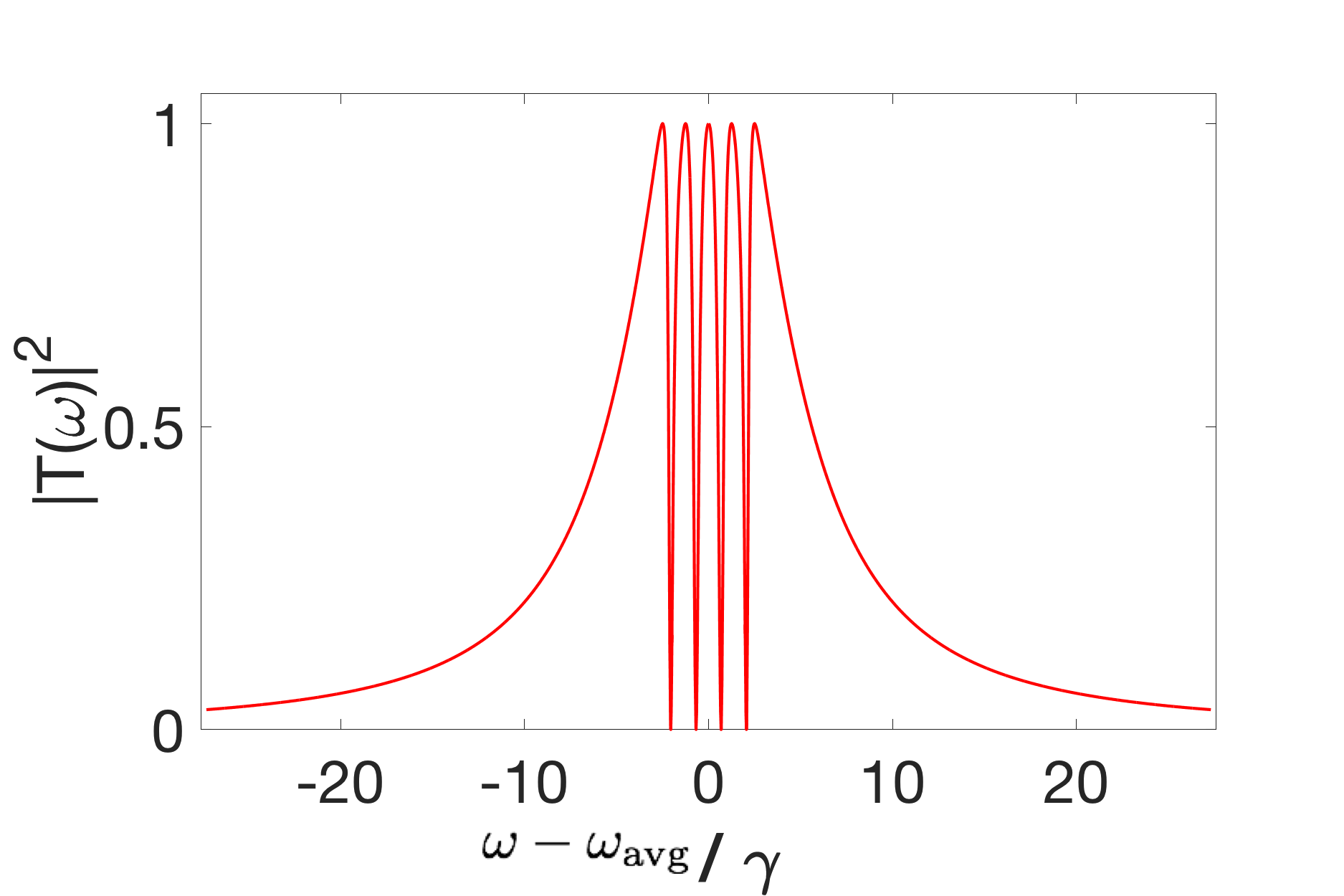
Figure 3.6: Transmission probability for a parallel network with ${N=5}$ equally spaced discrete states with balanced decay rates to both continua (${\gamma=\Gamma}$). Frequency is measured w.r.t. the average resonance frequency. We observe the five resonance frequencies $\omega_{i}$ each correspond to a perfectly transmitted frequency. The four frequencies of perfect refection correspond to solutions of ${\sum_{i}\frac{1}{\Delta_{i}}=0}$.

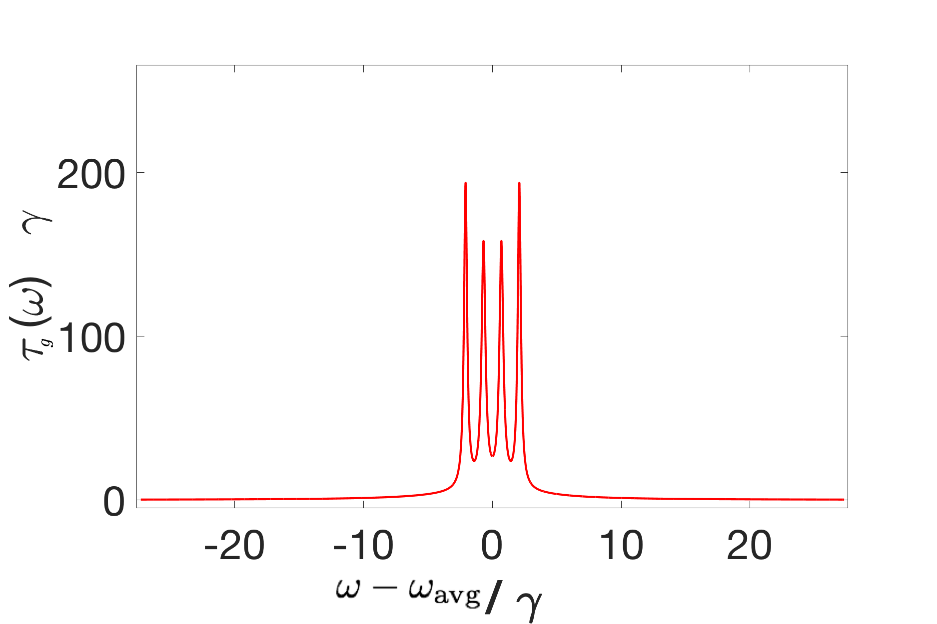
Figure 3.7: Group delay (in units of $\frac{1}{\gamma}$) for a parallel network with ${N=5}$ equally spaced discrete states with balanced decay rates to both continua (${\gamma=\Gamma}$). The group delay is always largest for the highest and lowest frequency resonances (except in the large spacing limit, where they are of equal magnitude).

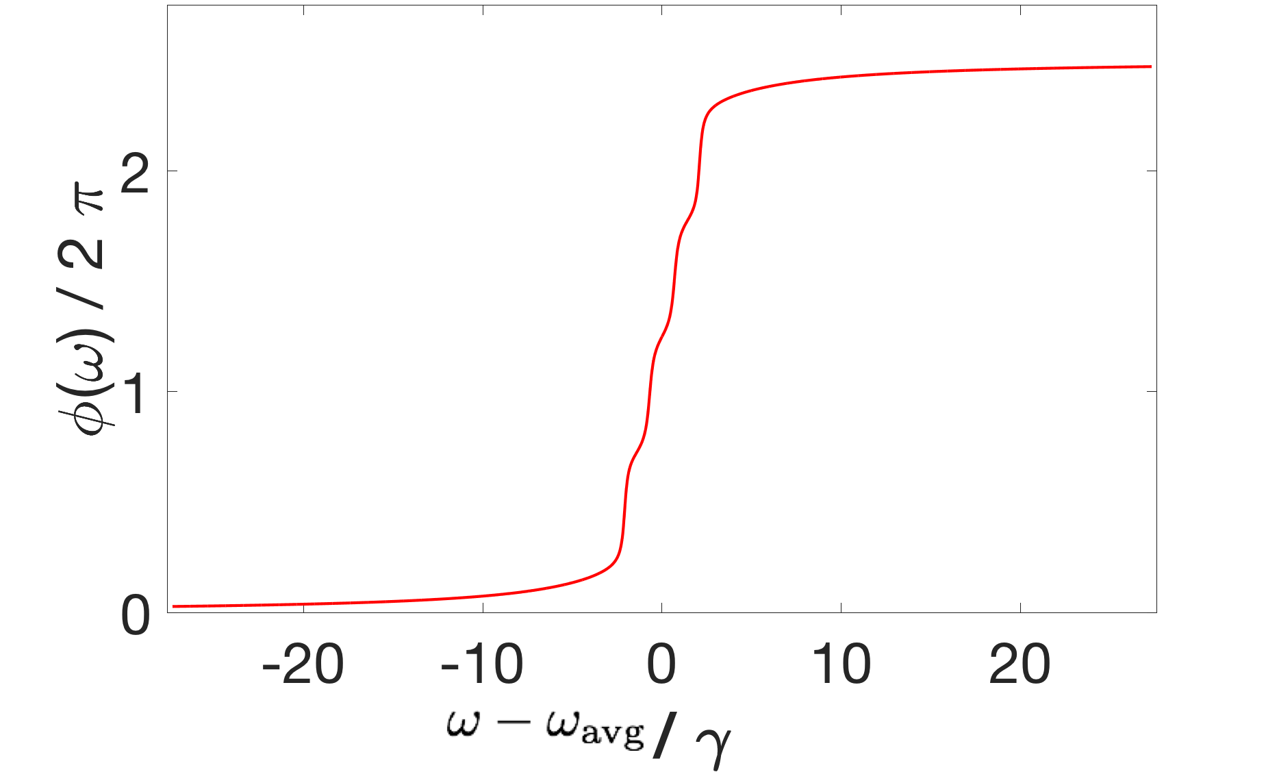
Figure 3.8: Transmission function phase (in units of $2\pi$) for a parallel network with ${N=5}$ equally spaced discrete states with balanced decay rates to both continua (${\gamma=\Gamma}$). The total change in phase of the transmission function is directly proportional to the number of discrete states. This is due to the phase shift in $\pi$ that occurs when crossing a resonance frequency, as was discussed for the simple example previously.

$$\frac{i\Delta_{i}}{\sqrt{\gamma_{i}}}c_{i}(\omega) =\sum\limits_{j}\frac{\sqrt{\gamma_{j}}(1+k)}{2}c_{j}(\omega)+a_{\rm in}(\omega)+\sqrt{k}\,b_{\rm in}(\omega)$$

so that we can identify strong correlations between discrete state amplitudes

$$\frac{i\Delta_{i}}{\sqrt{\gamma_{i}}}c_{i}(\omega)=\frac{i\Delta_{i^{\prime}}}{\sqrt{\gamma_{i^{\prime}}}}c_{i^{\prime}}(\omega).$$ (3.22)

For non-degenerate states, Eq. 3.22 means that a photon that is resonant with one state will only excite that state. (For infinitely-narrow discrete states, these correlations are satisfied trivially of course; $c_{i^{\prime}}(\omega)$ is only non-zero at $\omega_{i^{\prime}}$.) Eq. 3.22 also indicates that the relative phase of discrete state amplitudes is frequency dependent; when $\omega_{i}<\omega<\omega_{i^{\prime}}$, there is a relative phase of $\pi$ between $c_{i}$ and $c_{i^{\prime}}$. (Outside of photo detection, this purely virtual coupling provides a possible alternative explanation for the destructive interference present in atoms along a fiber [167, 168] and multi-mode Fabry-Perot cavities [169].) We can see destructive interference directly from the form of the reflection coefficient

$$R(\omega)=\frac{i-(k-1)\sum\limits_{i}\frac{\gamma_{i}}{2(\Delta_{i})}}{i-(k+1)\sum\limits_{i}\frac{\gamma_{i}}{2(\Delta_{i})}}$$ (3.23)

from which we can determine $|T(\omega)|^{2}$ and the other quantities of interest.

We can further specialize to the case of homogenous coupling where $\gamma_{i}=\gamma$ and $\Gamma_{i}=\Gamma$. This case is of interest for several reasons: most generally, this assumption directly follows from the first Markov approximation if the spacing between discrete states is small compared to the decays. It also simplifies the form of the correlations between discrete states $\Delta_{i}c_{i}(\omega)=\Delta_{i^{\prime}}c_{i^{\prime}}(\omega)$, as well as the form of the reflection coefficient

$$R(\omega)=\frac{i-\frac{\Gamma-\gamma}{2}\sum\limits_{i}\frac{1}{\Delta_{i}}}{i-\frac{\Gamma+\gamma}{2}\sum\limits_{i}\frac{1}{\Delta_{i}}}.$$ (3.24)

Perfect transmission.— From (3.23) and (3.24) we can see that in both cases there are $N$ frequencies of maximum transmission corresponding to each resonant frequency $\Delta_{i}=0$ with transmission probability $|T(\omega_{i})|^{2}=\frac{4k}{(k+1)^{2}}$ and $|T(\omega_{i})|^{2}=\frac{4\gamma\Gamma}{(\gamma+\Gamma)^{2}}$, respectively. We also see $N-1$ frequencies of destructive interference corresponding to the $N-1$ solutions of $\sum\limits_{i}\frac{\gamma_{i}}{\Delta_{i}}=0$ (Fig. 3.5) determined solely by the decays and resonances (and notably not by $k$). We similarly observe for the case of a network with homogenous decay rates $N-1$ frequencies of destructive interference corresponding to the solutions of $\sum\limits_{i}\frac{1}{\Delta_{i}}=0$ (Fig. 3.6). One might think that, in principle, a resonant frequency could coincide with a frequency of perfect reflection when $N>2$, in which case they can annihilate. However, this only occurs when two discrete states are energetically degenerate. Since the discrete states would also couple to the same $1$D continuum, this is forbidden by unitarity. To avoid this, we see a resonant frequency that is perfectly transmitted and a frequency of destructive interference move closer together as the spacing between discrete states is decreased. When the degeneracy becomes exact, a discrete state is forced to decouple from the system as the frequencies of perfect reflection and transmission annihilate.

In general, the condition for perfect transmission through a parallel network is that all the couplings be balanced ($\gamma=\Gamma$ or in the inhomogeneous uniformly balanced case, $k=1$). As we saw in the case for a completely arbitrary parallel network, we see that perfect transmission at some discrete state frequency $\omega_{i}$ not only requires balanced coupling $\gamma_{i}=\Gamma_{i}$, but also that all the other discrete states either be far away in frequency compared to the their decay rates ($|\omega_{i}-\omega_{j}|\gg\gamma_{j},\Gamma_{j}$), or also be balanced ($\gamma_{j}=\Gamma_{j}$), or a mix of the two.

Spectral Bandwidth.— Once we have the reflection coefficient, we can calculate the three quantities of interest. For all three cases we’ve discussed, we find that the spectral bandwidth is purely additive $\tilde{\Gamma}=\sum_{i}\frac{2\gamma_{i}\Gamma_{i}}{\gamma_{i}+\Gamma_{i}}$ and is completely independent of the spacing between discrete states.

Group Delay.— We note that, unlike the simple model, the sharp peaks in the group delay (Fig. 3.7) correspond to frequencies of destructive interference and are greatest for the outermost frequencies of destructive interference despite all the frequencies of note in (Fig. 3.6) being completely destructive or constructive. We also observe that the relationship between the three quantities of interest discussed for the simple model is not present: here $\tau_{g}(\omega_{i})>\tilde{\Gamma}^{-1}|T(\omega_{i})|^{2}$ for each resonant frequency. We find that the phase of $T(\omega)$ increases by $\pi$ with each resonant frequency (3.8). This provides a novel application for single-photon interferometry for resolving tightly-structured resonance structures and explains why, whereas the spectral bandwidth $\tilde{\Gamma}$ is independent of discrete state spacing, the group delay increases with close spacing; the same change in phase is occurring in a smaller spectral range so the magnitude of the group delay $|\tau_{g}(\omega)|=|\frac{d\phi(\omega)}{d\omega}|$ increases.

3.3.2 Series Networks

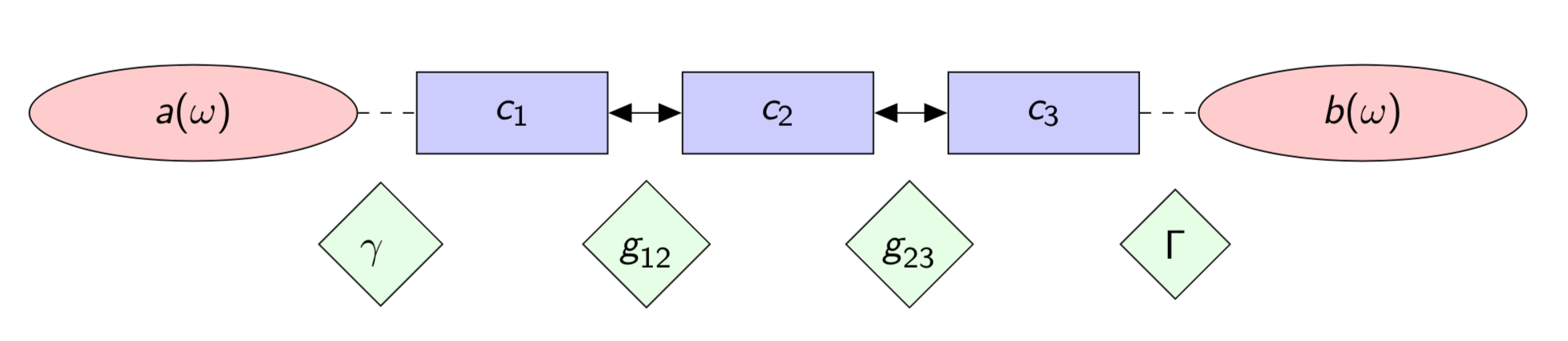
Figure 3.9: A series network of three coherently coupled discrete states, each described by an operator $c_{i}$ and coupled to each other at rates $g_{ij}$. The first and last states decay to left (input, external) and right (output, internal) continua $a$ and $b$ at rates $\gamma$ and $\Gamma$, respectively.

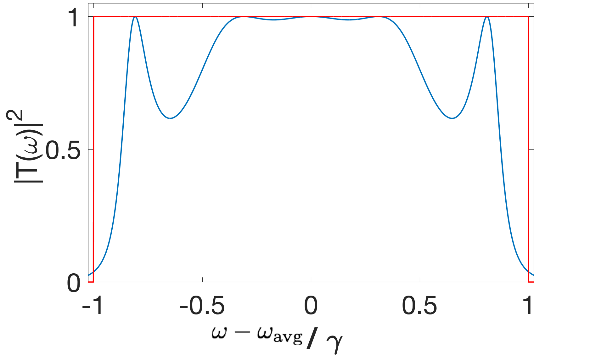
Figure 3.10: Transmission probability for a quantum network with ${N=5}$ discrete states in series with no relative detuning and balanced decay rates ${\gamma=\Gamma}$ for the special case of homogenous critical coupling ${g_{ij}\rightarrow g=\frac{\sqrt{\gamma\,\Gamma}}{2}}$. For comparison with the actual transmission probability (blue curve), we also plot a fictitious transmission probability (red bounding box) that is unity for ${-2g\leq\omega\leq 2g}$ and zero elsewhere. Frequencies are measured w.r.t. resonance. Meeting both the balanced decay and critical coupling conditions ensures that the on-resonance transmission is both unity and maximally broadened, but are not necessary conditions for perfect transmission to occur at some frequency.

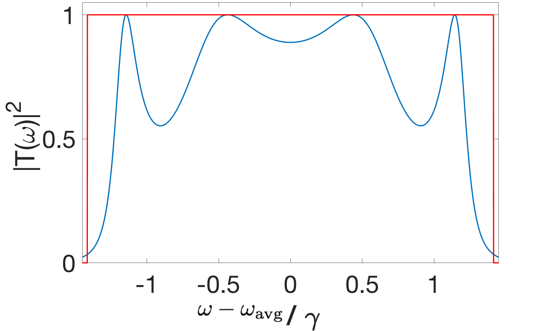
Figure 3.11: Transmission probability for a quantum network with ${N=5}$ discrete states in series with no relative detuning and unbalanced decay rates ${2\gamma=\Gamma}$ for the special case of homogenous critical coupling ${g_{ij}\rightarrow g=\frac{\sqrt{\gamma\,\Gamma}}{2}}$. Again, we observe perfect transmission for certain frequencies.

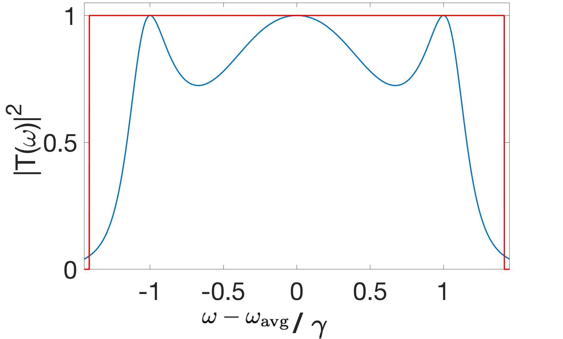
Figure 3.12: Transmission probability for a quantum network with ${N=4}$ discrete states in series with no relative detuning and unbalanced decay rates ${2\gamma=\Gamma}$, again for the special case of homogenous critical coupling ${g_{ij}\rightarrow g=\frac{\sqrt{\gamma\,\Gamma}}{2}}$ ensuring perfect transmission at some frequencies

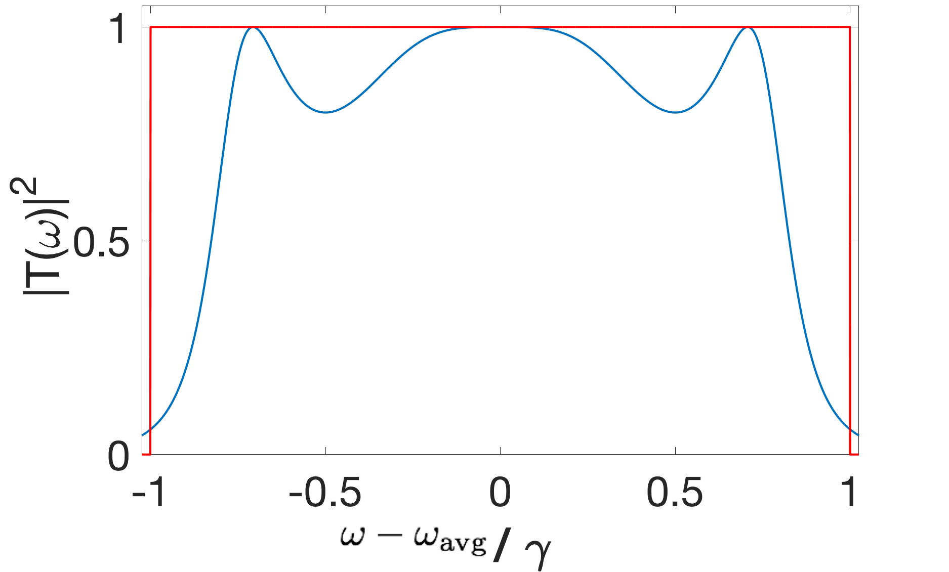
Figure 3.13: Transmission probability for a quantum network with ${N=4}$ discrete states in series with no relative detuning and balanced decay rates ${\gamma=\Gamma}$. Here critical coupling ${g_{ij}\rightarrow g=\frac{\sqrt{\gamma\,\Gamma}}{2}}$ ensures both perfect transmission and maximal broadening on-resonance.

In general, we cannot diagonalize a completely arbitrary network in terms of a single set of parallel states; there may be a causal relationship embedded in the network structure; for example, for an atom in an s-state coupled via a photon to one or many p-states which subsequently decay to multiple d-states, we would have to diagonalize the p-states and d-states separately. A class of such systems are series quantum networks (Fig. 3.9), where only one state is coupled to each continuum, with the other states forming a chain between the two outer ones ($\gamma_{i>1}=0$, $\Gamma_{i<N}=0$, and $g_{ij}=0$ for $j\neq i\pm 1$). This provides a natural (and especially simple) model for energy transport and repeated spectral filtering (a series of Fabry-Perot cavities). Furthermore, we can analytically determine the transmission function for arbitrary series networks, as we will now proceed to do.

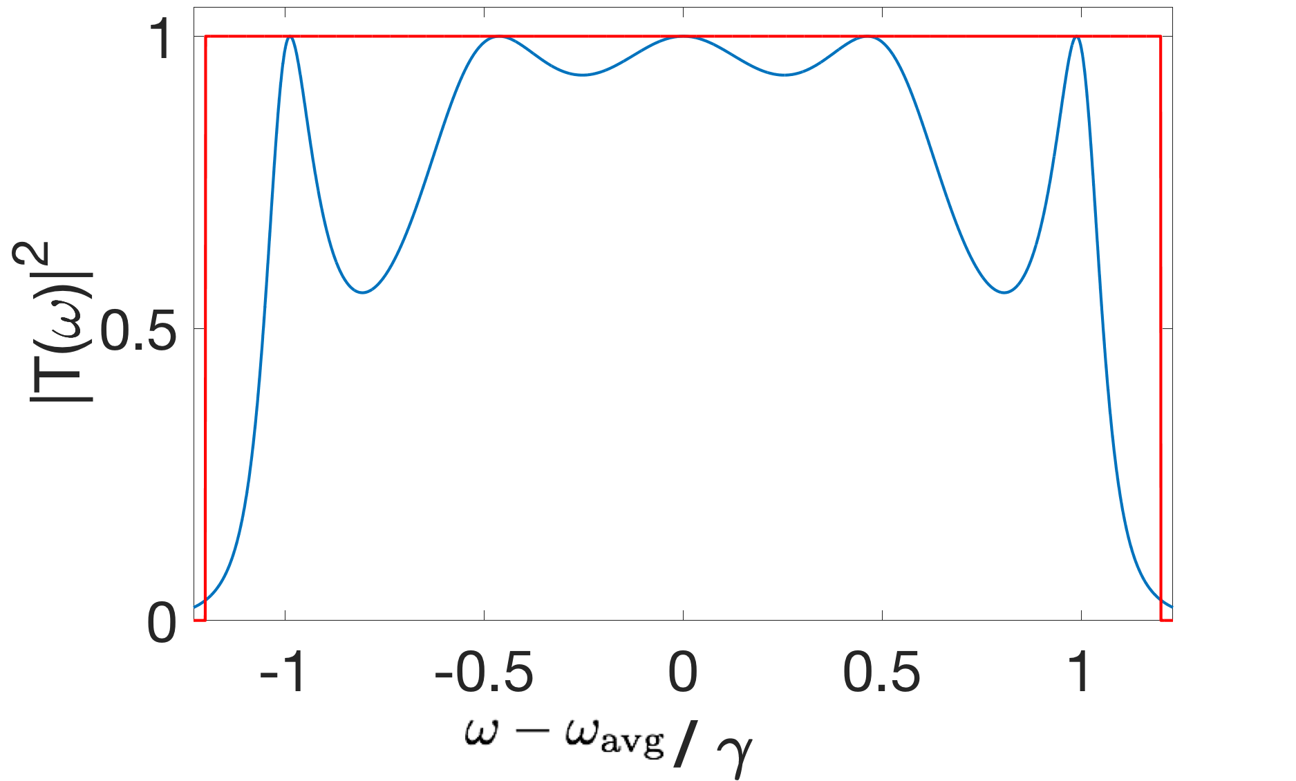
Figure 3.14: Transmission probability for networks with ${N=5}$ discrete states in series with no relative detuning for the special case of homogenous balanced decays ${\gamma=\Gamma}$ (blue curve) and over-coupling ${g=\frac{6}{5}\frac{\sqrt{\gamma\Gamma}}{2}}$. A balanced over-coupled network will always have more peaks of perfect transmission than an under-coupled or critically-coupled one, though on-resonance transmission may not be a local maxima.

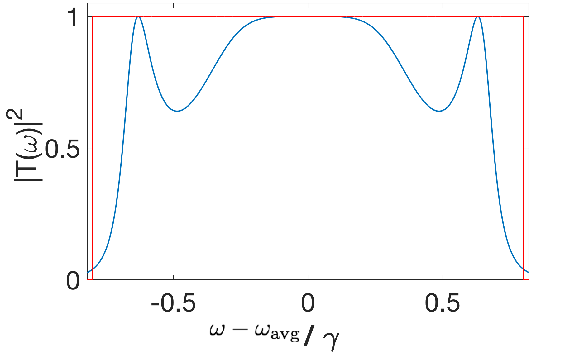
Figure 3.15: Transmission probability for networks with $N=5$ discrete states in series with no relative detuning for the special case of homogenous balanced decays ${\gamma=\Gamma}$ (blue curve) and under-coupling ${g=\frac{4}{5}\frac{\sqrt{\gamma\Gamma}}{2}}$.

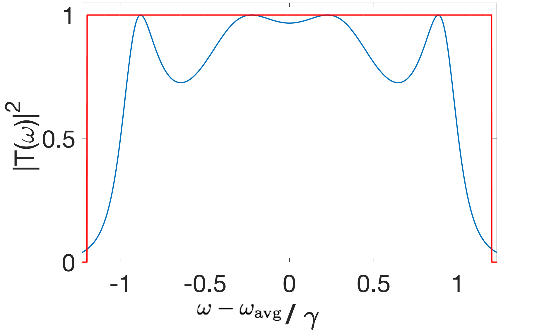
Figure 3.16: Transmission probability for networks with ${N=4}$ discrete states in series with no relative detuning for the special case of homogenous balanced decays ${\gamma=\Gamma}$ (blue curve) and over-coupling ${g=\frac{6}{5}\frac{\sqrt{\gamma\Gamma}}{2}}$. Again, balanced over-coupled network will always have more peaks of perfect transmission than an under-coupled or critically-coupled one, though on-resonance transmission may not be a local maxima.

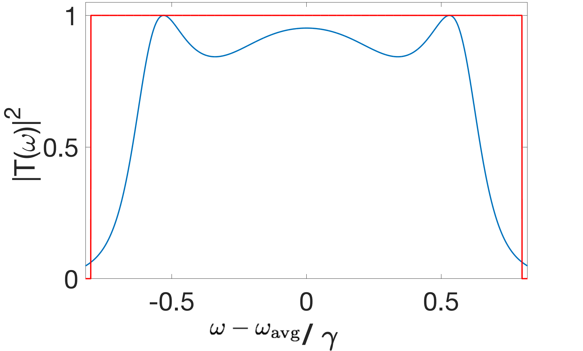
Figure 3.17: Transmission probability for networks with ${N=4}$ discrete states in series with no relative detuning for the special case of homogenous balanced decays ${\gamma=\Gamma}$ (blue curve) and under-coupling ${g=\frac{4}{5}\frac{\sqrt{\gamma\Gamma}}{2}}$.

Since each state is only coupled to the two adjacent states, the system of $N$ equations of the form of (3.16) describing evolution of the system is solvable in a stepladder-type approach. Setting the expectation value of the second input continuum to zero, we solve for the $N$th state in terms of the $N-1$th. As we step up the ladder, we find that the expression for the reflection coefficient has the form of a generalized continued fraction

$$R(\omega) =1-\cfrac{\gamma}{\frac{\gamma}{2}-i\Delta_{1}+\cfrac{g_{12}^{2}}{-i\Delta_{2}+\cfrac{g_{23}^{2}}{\dots+\cfrac{g_{N-1N}^{2}}{\frac{\Gamma}{2}-i\Delta_{N}}}}}$$ (3.25)

(we have dropped the subscripts on $\gamma_{1}$ and $\Gamma_{N}$). This equation looks difficult to analyze, but can be greatly simplified using the Wallis-Euler recursion relations for continued fractions. We define two function $A_{n}$ and $B_{n}$ given by the following recurrence relations

$$B_{-1}=0,B_{0}=1,A_{-1}=1,A_{0}=b_{0}$$

$$A_{n}=b_{n}\,A_{n-1}+a_{n}\,A_{n-2}\,(n\geq 1)$$

$$B_{n}=b_{n}\,B_{n-1}+a_{n}\,B_{n-2}\,(n\geq 1)$$ (3.26)

with coefficients $a_{n}$ and $b_{n}$ given in Tbl. 3.1. The reflection coefficient is then given $R(\omega)=\frac{A_{N}}{B_{N}}$ for $N$ discrete states. (For $n<N$, the functions $A_{n}$ and $B_{n}$ have no clear physical meaning.) From this, we easily solve for conditions where $R(\omega)=0$ (perfect transmission).

$n$	$a_{n}$	$b_{n}$
$0$	$0$	$1$
$1$	$-\gamma$	$\frac{\gamma}{2}-i\,\Delta_{1}$
$2$	$g_{12}^{2}$	$-i\,\Delta_{2}$
$\vdots$	$\vdots$	$\vdots$
$N-1$	$g_{N-2N-1}^{2}$	$-i\,\Delta_{N-1}$
$N$	$g_{N-1N}^{2}$	$\frac{\Gamma}{2}-i\,\Delta_{N}$
$>N$	$0$	$0$

Table 3.1: Wallis-Euler coefficients for ${N>1}$ discrete states in series. For a series network with an arbitrarily high number of discrete states $N$, these can be used to generate transmission functions (that correctly encode the causal structure that is inherent to the network outside of the strong-coupling limit) using the Wallis-Euler recursion relations (3.3.2).

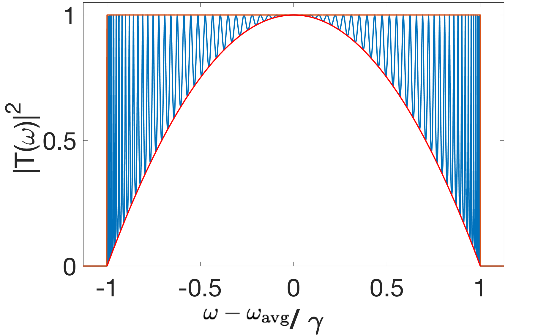
Figure 3.18: Transmission probability for a series network with ${N=70}$ identical discrete states (${\omega_{i}=\omega_{j}}$) with both balanced decays (${\gamma=\Gamma}$) and uniform critical coupling (${g=\frac{\sqrt{\gamma\Gamma}}{2}}$) conditions met. This results in a maximally-broadened on-resonance transmission. In the large-$N$ limit, the amplitude of this ideal (perfect and broadened) transmission function $|T(\omega)|$ is bounded below by a circle (parabola for $|T(\omega)|^{2}$) and above by a square (both red) with widths $2g$ and maxima of unity.

Perfect transmission.— We begin by considering the unphysical but illuminating case of an infinite series of identical discrete states ($g_{i\,i+1}=g\,\forall i$ and $\Delta_{i}=\Delta\,\forall i$) analytically. We find that the limit $\lim_{N\rightarrow\infty}R(\omega)$ only converges on-resonance for the special “critical” case

$$g=\frac{\sqrt{\gamma\,\Gamma}}{2}.$$ (3.27)

Furthermore, the limit only converges to zero on resonance (perfect transmission) when we also have $\gamma=\Gamma$. This first condition corresponds to a series of discrete states coupled through their decays (e.g. Fabry-Perot cavities coupled through their evanescent fields), and the second condition corresponds to the same requirement of balanced decays we saw for parallel quantum networks.

While infinite series networks of discrete states are not realistic, these two conditions play different but important roles in all finite series networks where the discrete states are identical (though introducing relative detuning will change the critical values of $g$ and $\Gamma/\gamma$, as we will see). That there are two conditions can be explained thus; since $R(\omega)$ is in general complex, the condition $R(\omega)=0$ gives two constraint equations on the real and imaginary parts of $R(\omega)$. When $N$ is even [odd], the real part is an order $N$ [$N-1$] polynomial in the detunings $\Delta_{i}$, while the imaginary part is order $N-1$ [$N$]. In general, this means there are conditions for a minimum of $N-1$ frequencies of perfect transmission and we may find $N$ frequencies of perfect transmission only if the lower-order equation is satisfied trivially for all frequencies. When considering finite series networks of identical discrete states, these same two conditions appear in the constraint equations for perfect transmission.

We now explore in detail the effects of these two conditions on series networks of identical discrete states with uniform coupling; first, consider fixing the coupling $g$ to be critical ($g=\frac{\sqrt{\gamma\Gamma}}{2}$). For odd $N$, we find that when the decays are balanced ($\gamma=\Gamma$), this ensures $N$ frequencies of perfect transmission (Fig. 3.10) with the resonance frequency at a local maxima of unity, and when the decays are unbalanced ($\gamma\neq\Gamma$), $N-1$ frequencies of perfect transmission (Fig. 3.11) with the resonant frequency at a local minima. For even $N$, letting $g=\frac{\sqrt{\gamma\Gamma}}{2}$ always results in $N-1$ frequencies of perfect transmission (Fig. 3.12) with the on-resonant frequency at a local maxima. Here, having balanced decays broadens the the on-resonance maxima (Fig. 3.13), which will be desirable for detection of non-monochromatic photons (wavepackets).

Now we instead consider balanced decays ($\gamma=\Gamma$) and observe a switch in the on-resonance behavior; whereas above we found that for even $N$ the critical coupling condition was sufficient for on-resonance transmission to be at a local maxima, we now find that, for odd $N$ that the balanced decay condition results in $N$ peaks of unity transmission (Fig. 3.14) with on-resonance transmission at a local maxima. Here three peaks become degenerate to give $N-2$ frequencies of perfect transmission when $g\lesssim\frac{\sqrt{\gamma\Gamma}}{2}$ (Fig. 3.15). (This inequality rapidly becomes exact [$g<\frac{\sqrt{\gamma\Gamma}}{2}$] with increasing $N$.) Similarly, for even $N$ we find the behavior of $T(\omega)$ depends strongly on the coupling, flipping between $N$ frequencies of perfect transmission with on-resonance transmission at a local minima for $g>\frac{\sqrt{\gamma\Gamma}}{2}$ (Fig. 3.16) and $N-2$ frequencies of perfect transmission with on-resonance transmission at a non-unity local maxima for $g<\frac{\sqrt{\gamma\Gamma}}{2}$ (Fig. 3.17).

For both even and odd $N$, the width is increasingly determined by $g$ with increasing $N$, with the half-width asymptotically approaching $2g$. In the large-$N$ limit, we observe that the transmission function is asymptotically bounded between a circle and a square when both conditions for perfect transmission are met (Fig. 3.18). We also observe that increasing $g$ past $\frac{\sqrt{\gamma\,\Gamma}}{2}$ while maintaining $\gamma=\Gamma$ induces Rabi splitting, with the $N$ or $N-1$ frequencies of perfect transmission spreading outwards (for odd and even $N$, respectively). For the special case of $N=2$, the presence of a second coupled discrete state resulting in a splitting and shift of the resonant frequency is in agreement with the effect seen in Ref. [20] for an antireflective coating; perfect transmission is still possible provided $\gamma=\Gamma$ but the frequency that is perfectly transmitted is split in to two.

In the strong coupling (high-$g$) limit, a frequency-comb structure emerges (Fig. 3.19), with dips approaching perfect reflection. This is due to the asymptotic irrelevance of the causal ordering (that is, the order in which an excitation must traverse discrete states to pass from one continuum to the other): the network becomes approximately diagonalizable as parallel modes with purely virtual coupling and the $N-1$ frequencies of perfect reflection from (3.23) manifest.

We now consider the effects of introducing relative detunings between discrete states as, generally, a quantum network will not be comprised of identical states. Still there are sufficient degrees of freedom in (3.25) such that, by tuning the parameters, perfect transmission at some frequencies is always possible. This is even true when $\gamma\neq\Gamma$ (for $N>1$): considering only two discrete states in series, we find that perfect transmission occurs at a frequency $\omega=\frac{\omega_{1}+\omega_{2}}{2}+\frac{\Gamma\omega_{1}-\gamma\omega_{2}}{\Gamma-\gamma}$ when $g_{12}=\sqrt{\frac{\gamma\Gamma}{4}+\left(\frac{\Gamma\omega_{1}-\gamma\omega_{2}}{\Gamma-\gamma}\right)^{2}-\left(\frac{\omega_{1}-\omega_{2}}{2}\right)^{2}}$ (Fig. 3.20). For two detuned discrete states in series with balanced decays ($\gamma=\Gamma$), perfect transmission is impossible as the critical value of $g$ is infinite; the transmission efficiency asymptotically becomes perfect in the strong-coupling limit. However, this a special case and is not true for larger numbers ($N>2$) of discrete states. Critically, given a series network of $N$ discrete states with arbitrary relative detunings, we can always find at least one set of parameters (couplings and decay rates) such that $N-1$ frequencies are perfectly transmitted.

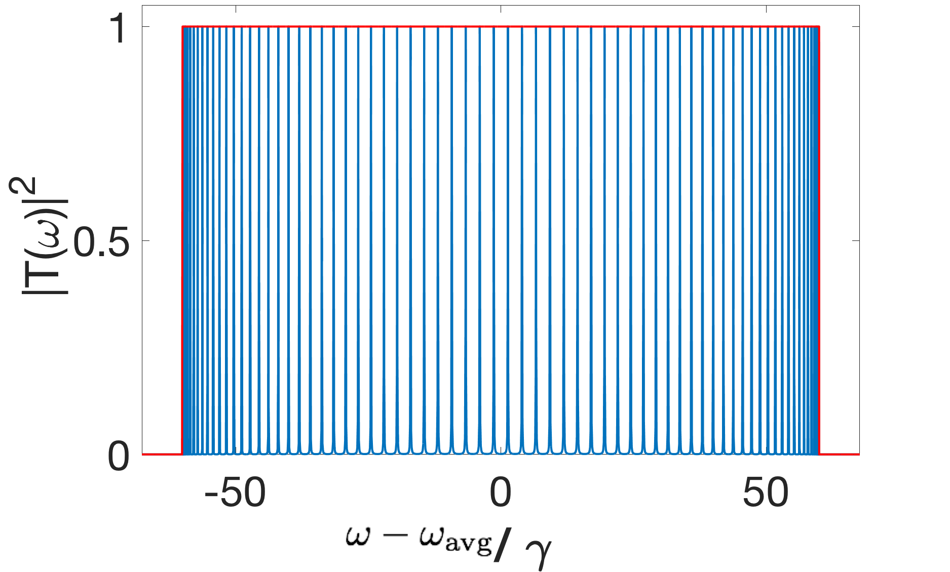
Figure 3.19: Transmission probability for a series network with ${N=70}$ identical discrete states with balanced decays (${\gamma=\Gamma}$) yielding perfect transmission in the strong-and-uniform coupling limit (${g\gg\frac{\sqrt{\gamma\Gamma}}{2}}$). The result is a frequency-comb structure with $70$ frequencies of unity transmission between $-2g$ and $2g$, separated by $69$ regions of near-perfect reflection.

Spectral Bandwidth.— Once we have the form of the transmission function, we can calculate the spectral bandwidth for these systems. The spectral bandwidth decreases with additional discrete states and is strictly bounded above by the single discrete state bandwidth $\tilde{\Gamma}\leq\frac{2\gamma\Gamma}{\gamma+\Gamma}$. For discrete states without detuning, equality is reached in the strong-coupling limit of $g\gg\frac{\sqrt{\gamma\Gamma}}{2}$ but independently of whether $\gamma=\Gamma$ (Fig. LABEL:tildeGammaN1). Introducing detuning between discrete states lowers the bandwidth, but equality with the upper limit still occurs for sufficiently strong coupling (Fig. LABEL:N1RelativeBandwidthDetuning); the strong coupling is able to better mask the discrepancy between discrete state frequencies as the dressed states become the more physical description and as the system more strongly resembles a parallel network. (In this limit, each dressed state is coupled to the continua at reduced decays so that the total bandwidth is still bounded by $\tilde{\Gamma}\leq\frac{2\gamma\Gamma}{\gamma+\Gamma}$ with $\gamma$ and $\Gamma$ the two original decay rates for the series network.)

Group Delay.— Lastly, we consider the group-delay for series networks, which increases with both $g$ and $N$ but for different reasons. As $g$ increases, the peaks of the transmission function sharpen so that the phase changes more rapidly. This results in an increased group delay (Fig. LABEL:2discretestatesSeriesTrans-d). As $N$ increase, we observe (as we did for parallel networks) that the peaks in the group delay are not of uniform magnitude, even when the transmission function itself is rather flat (Fig. LABEL:20discretestatesSeriesTrans). Instead, the frequencies of maximum delay are those closest to $\pm 2g$ (Fig. LABEL:20discretestatesSeriesTau) and increase the most with $N$. This is because the oscillations in the transmission function are most dense here, resulting in a rapid change in transmission function phase and thus a larger group delay. On the contrary, the group delay is relatively flat in the center of the transmission window (Fig. LABEL:20discretestatesSeriesTau) so that a spectrally-narrow (compared to $g$) input photon pulse will not be significantly dispersed. (That is, the maximum dispersion-induced jitter $\mathcal{T}_{g}$ from (3.5) will be very small.)

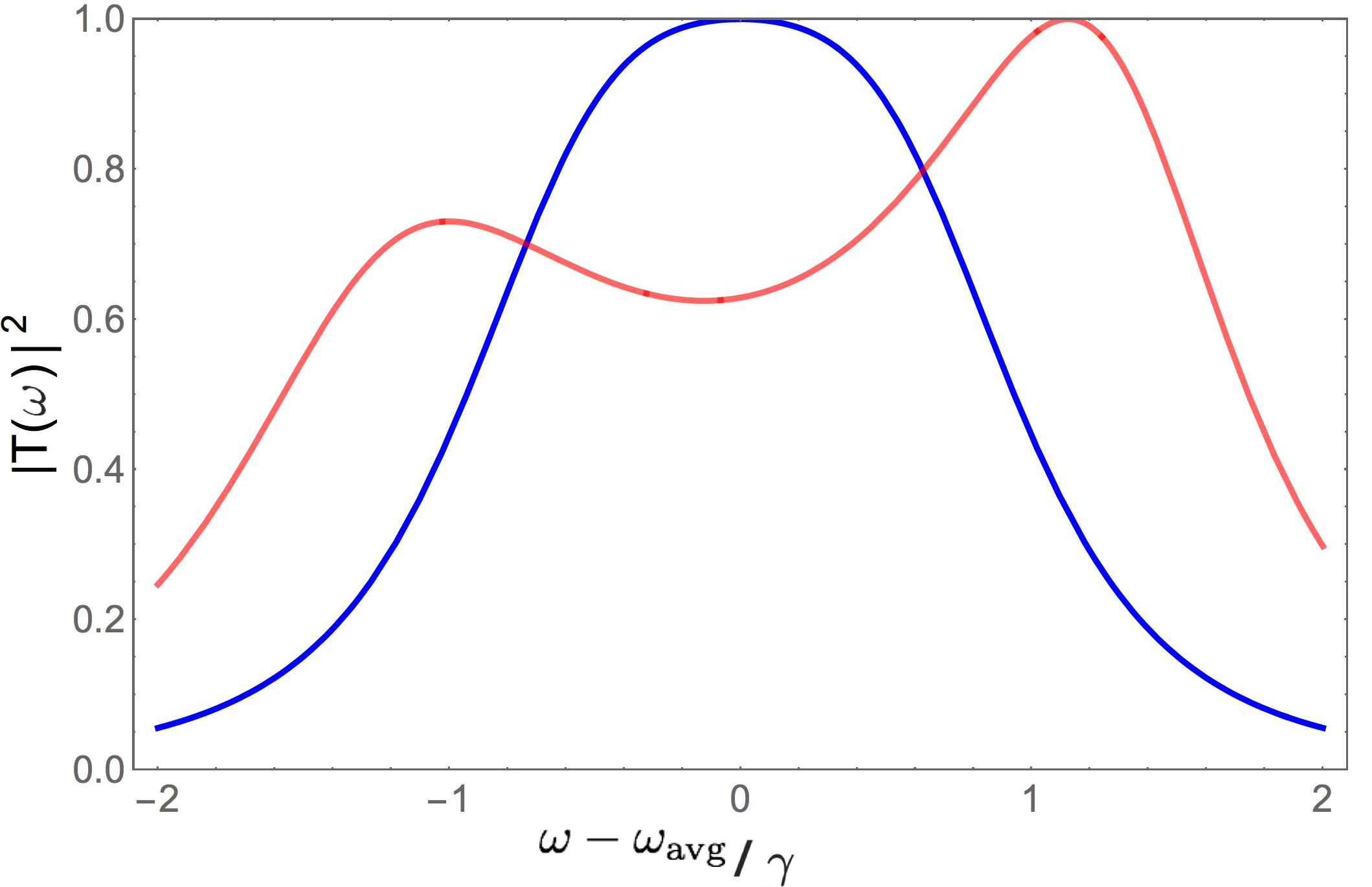
Figure 3.20: Transmission probabilities for series networks with ${N=2}$ discrete states with no relative detuning (blue with a single maxima), and with non-zero relative detuning ${\frac{\omega_{2}-\omega_{1}}{\gamma}=\frac{3}{4}}$ (red with two maxima). In both cases, the decays are not balanced (${\frac{\Gamma}{\gamma}=2}$) but the couplings are chosen such that perfect transmission at some frequency is achieved nonetheless.

We can also consider the effect of detunings on the frequency-dependent group delay. We observe the group delay can be negative for series networks with detuning (Fig. LABEL:DetunedN20Tau), with an asymmetric structure that depends on the ordering of the detunings (except in the strongly coupled limit) . Again, the magnitude of the group delay depends on the spacing of discrete states, increasing when the resonant frequencies are closely spaced.

3.3.3 Hybrid Networks

Figure 3.21: A hybrid network of two manifolds, each with $N_{k}$ discrete states described by operators $c^{(k)}_{i}(\omega)$ where the index $k$ here has only two values (${k=1,\,2}$). The discrete states are coherently coupled at rates $g^{(1,2)}_{ij}$ and incoherently coupled to left (input, external) and right (output, internal) continua $a$ and $b$ with decay rates $\gamma^{(1)}_{i}$ and $\Gamma^{(2)}_{j}$, respectively. Each discrete state is part of a manifold: a set of discrete all coupled to the same state and continua (but not necessarily at the same rate).

We now begin to approach the case of a general two-sided quantum network. The fully general problem is intractable analytically, but luckily there are several simplifications we can make that correspond to the network representing realistic photo detecting systems. To illustrate, consider the case of two parallel networks in series: each discrete state connected to each discrete state in the other manifold (but not necessarily at the same rate) with each of the two manifolds of purely virtually coupled discrete states coupled to their own continuum. One could imagine generating different networks from this one by removing a coupling $g_{ij}$ between discrete states, permuting which discrete states are disconnected, removing an additional coupling, permuting, and so on. However, this is unphysical! Two discrete states in parallel cannot be prevented from coupling to the same discrete state except by selection rules, this would violate unitarity! But the discrete states are also coupled to the same continuum which has the same quantum numbers associated with it (we have removed other degrees of freedom in going to the $1D$ problem), so they must satisfy the same selection rules. The same argument applies in reverse: no discrete state within a manifold can individually stop being coupled to a continuum without the rest of the discrete states doing so as well. This argument also applies to manifolds embedded in a larger network away from any continuum, the requirement that all states satisfy the same selection rules is very strong. As a result, in our analysis we can ignore partially connected networks, they are unphysical! It also gives us a helpful way to organize discrete states, into manifolds of purely virtually coupled discrete states (after diagonalization) that are all coupled to the same set of discrete states and/or continua.

We can now focus on a very large class of quantum networks, hybrid systems consisting of manifolds in series (Fig. 3.21). It will be helpful to denote couplings between discrete states $i$ and $j$ or manifolds $k$ and $\ell$ as $g_{ij}^{(k,\ell)}$, and denote decay rates and discrete states within a manifold with a superscript ($\gamma_{i}^{(k)}$, $\Gamma_{i}^{(k)}$, and $c_{i}^{(k)}(\omega)$, with $\gamma_{i}^{(k)}=0$ for $k>1$ and $\Gamma_{i}^{(k)}=0$ for $k<M$, where $M$ is the number of manifolds). This allows us to rewrite the general equation (3.16) in a more explicit form

$$-i\Delta_{i}c_{i}^{(k)}(\omega)= -\sum\limits_{j=1}^{N_{k}}\frac{\sqrt{\gamma_{i}^{(k)}\gamma_{j}^{(k)}}+\sqrt{\Gamma_{i}^{(k)}\Gamma_{j}^{(k)}}}{2}c_{j}^{(k)}(\omega)-i\sum\limits_{j=1}^{N_{k-1}}g_{ij}^{(k-1,k)}c_{j}^{(k-1)}-i\sum\limits_{j=1}^{N_{k+1}}g_{ij}^{(k,k+1)}c_{j}^{(k+1)}$$ (3.28)

$$-\sqrt{\gamma_{i}^{(k)}}a_{\rm in}(\omega)-\sqrt{\Gamma_{i}^{(k)}}b_{\rm in}(\omega)$$

where the superscripts denote labels of manifolds and we’ve implicitly defined $g_{ij}^{(0,1)}=g_{ij}^{(N,N+1)}=0\,\forall i,j$. We denote the number of discrete states in each manifold $N_{k}$ such that $\sum\limits_{k=1}^{M}N_{k}=N$. In general (3.28) is still only numerically solvable but we can now note two cases that yield analytic solutions.

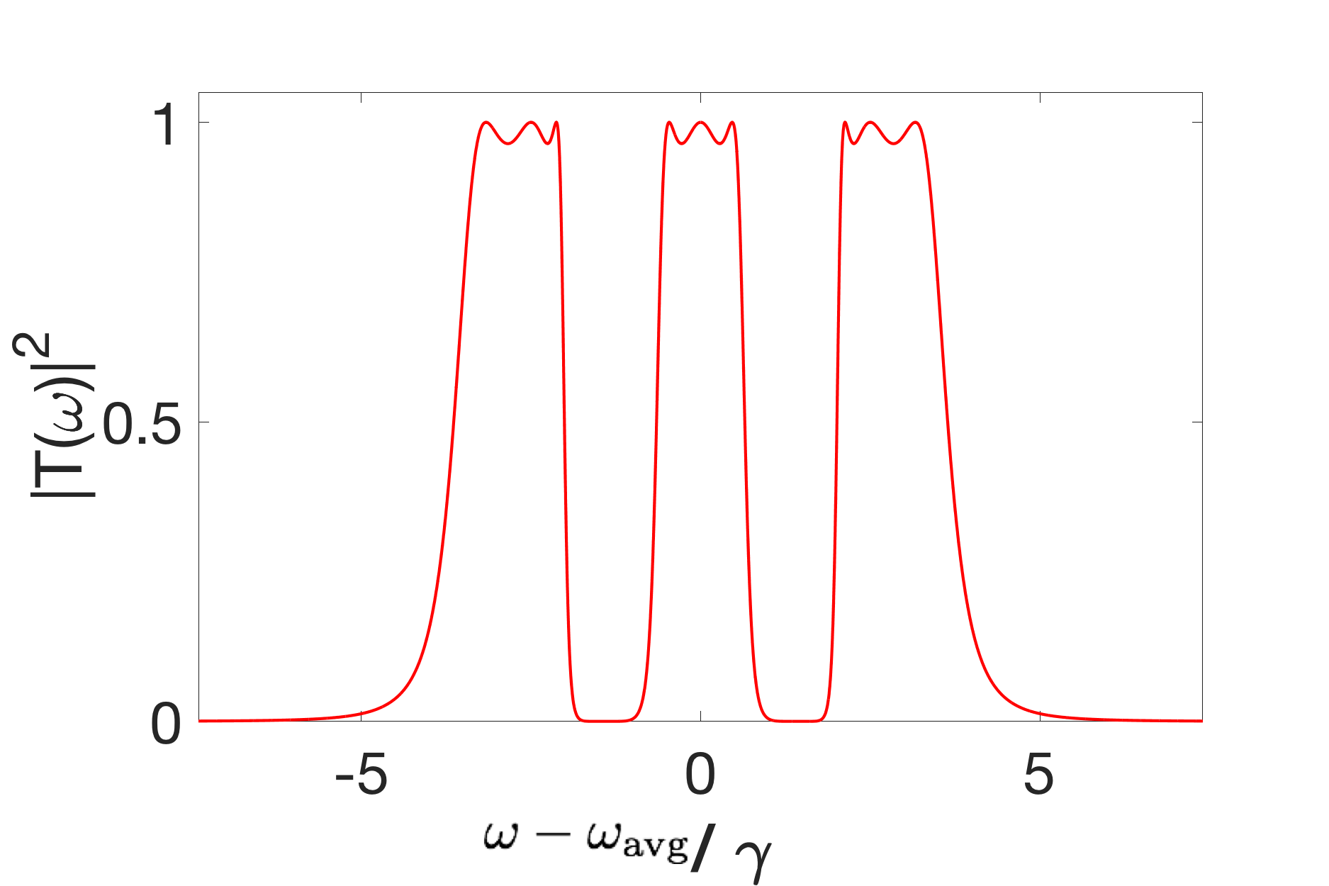
Figure 3.22: Transmission probability for a hybrid network consisting of $3$ manifolds in series, each with $3$ discrete states with balanced decays and uniform critical coupling. Within each manifold, the discrete states have frequency spacing by $2.5\gamma$. Using the same special conditions as for series network, perfect transmission is achieved for $9$ frequencies, with the multi-layered structure of $|T(\omega)|^{2}$ encoding the manifold structure.

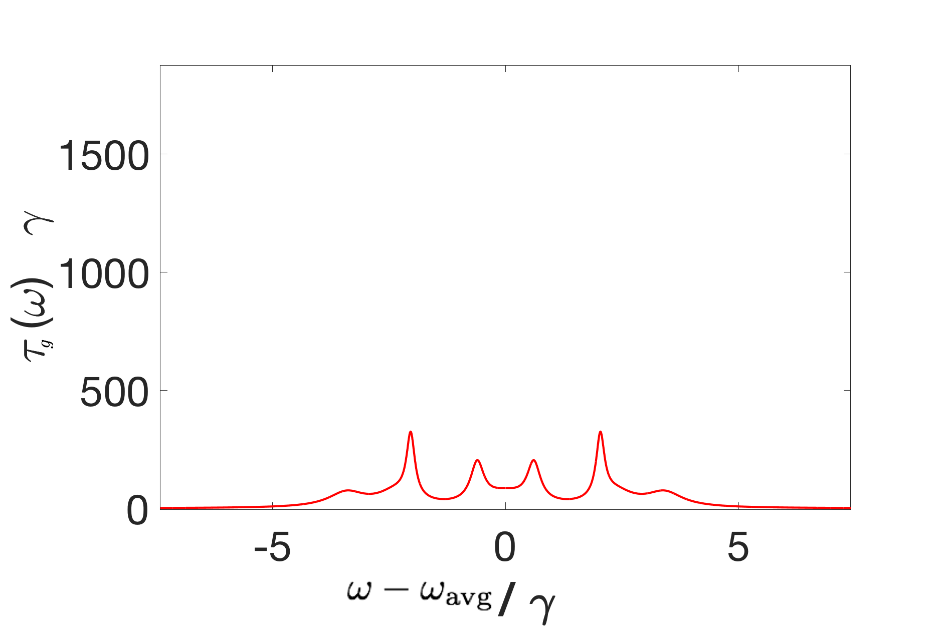
Figure 3.23: Group delay for a hybrid network consisting of $3$ manifolds in series, each with $3$ discrete states with balanced decays and uniform critical coupling, the transmission function of which is given in Fig. 3.22. Within each manifold, the discrete states have frequency spacing by $2.5\gamma$.

The first is the case of critical coupling between members of each adjacent manifold and, additionally, uniformly unbalanced decays: we first define an effective decay rate for internal couplings within the system so that $g_{ij}^{(k,\ell)}=\frac{\sqrt{\gamma_{i}^{(k)}\Gamma_{j}^{(\ell)}}}{2}$ (effectively specializing to the critical coupling case for series networks), and then consider the special case of $\Gamma_{i}^{(k)}/\gamma_{i}^{(k)}=k^{(k)}\,\forall i,k$ (inhomogeneous decays that are uniformly unbalanced within each manifold). This leads to a reflection coefficient of the form

$$R(\omega) =1-\cfrac{2h^{(1)}}{h^{(1)}-i+\cfrac{k^{(1)}h^{(1)}h^{(2)}}{-i+\cfrac{k^{(2)}h^{(2)}h^{(3)}}{\dots+\cfrac{k^{(N-1)}h^{(N-1)}h^{(N)}}{\sqrt{k^{(N)}}h^{(N)}-i}}}}$$

where we have defined a new function $h^{(k)}=\sum\limits_{i=1}^{N_{k}}\frac{\gamma_{i}^{(k)}}{2\Delta_{i}^{(k)}}$. (The appearance of a lone $\sqrt{k^{(N)}}$ at the end of (LABEL:refseriesc1) is due to the final purely virtual coupling to the output continuum, since we’ve absorbed the rest of the decay rate into the function $h^{(k)}$.) This function encodes the zeroes and singularities we found for parallel networks, which previously gave rise to frequencies of constructive interference and completely destructive interference.

While (LABEL:refseriesc1) is tractable, it is of limited applicability to real systems. More relevant is the second solvable case of homogenous coupling and decays within manifolds: $g_{ij}^{(k,\ell)}=g^{(k,\ell)}$, $\gamma_{i}^{(k)}=\gamma^{(k)}$, and $\Gamma_{i}^{(k)}=\Gamma^{(k)}$. This leads to a reflection coefficient of the form

$$R(\omega) =1-\cfrac{\gamma f^{(1)}}{\frac{\gamma}{2}f^{(1)}-i+\cfrac{(g^{(1,2)})^{2}f^{(1)}f^{(2)}}{-i+\cfrac{(g^{(2,3)})^{2}f^{(2)}f^{(3)}}{\dots+\cfrac{(g^{(N-1,N)})^{2}f^{(N-1)}f^{(N)}}{\frac{\Gamma}{2}f^{(N)}-i}}}}$$

where again we have defined a new function $f^{(k)}=\sum\limits_{i=1}^{N_{k}}\frac{1}{\Delta_{i}^{(k)}}$. This provides a nice model for multi-mode systems in series (for instance, a linear network of identical multimode optical cavities; in this case, the critical coupling strength $g=\frac{\sqrt{\gamma\Gamma}}{2}$ corresponds to optical cavities perfectly coupled through their decays).

We see in both (LABEL:refseriesc1) and (LABEL:refseriesc2) a combination of the structures we observed in (3.23) and (3.24) for parallel networks and (3.25) for series networks: correlations in amplitudes between discrete states within a given manifold manifest via a function $h^{(k)}$ or $f^{(k)}$ with $N_{k}$ poles and $N_{k}-1$ zeroes (potentially perfectly transmitted and reflected frequencies, depending on the hybrid network’s resonance structure and couplings), and causal ordering of the manifolds manifests in a continued fraction structure. This latter property makes them easily analyzable using the Wallis-Euler recurrence relations, allowing us to find $R(\omega)$ and from there $T(\omega)$ and the other quantities of interest.

Perfect transmission.— Focusing on the case of homogenous coupling, we can use the same trick of examining the convergence of an infinite series of identical manifolds around one of resonant frequencies $\omega_{i}$ to find the two critical conditions as we did for series networks, which again are $\gamma=\Gamma$ and $g=\frac{\sqrt{\gamma\Gamma}}{2}$. We also observe that the form of $T(\omega)$ for hybrid systems exhibits a combination of features of series and parallel networks (Figs. 3.22, 3.24, and 3.26). This results in layers of structure, with the small dips and peaks corresponding to intra-manifold structure layered on top of the larger dips and peaks of the inter-manifold structure.

When at least one discrete state from each of the manifolds have the same resonance frequency, letting $\gamma=\Gamma$ and $g=\frac{\sqrt{\gamma\Gamma}}{2}$ ensures perfect transmission at $M$ frequencies. For a general hybrid network, the number of peaks of unity (perfect transmission) of $T(\omega)$ are bounded above by $M\times{\rm Min}\{N_{k}\}\leq N$, with $M$ the number of manifolds and $N_{k}$ the number of discrete states in the $k$th manifold. Here the latter equality is reached for networks that are completely in parallel or completely in series, with critical parameters in either case.

Spectral Bandwidth.— For hybrid networks where the first and last manifold have the same number of discrete states $N_{1}=N_{M}$, the spectral bandwidth is bounded above by the parallel network bandwidth for that number of discrete states $\tilde{\Gamma}\leq\frac{N_{1}2\gamma\Gamma}{\gamma+\Gamma}$ with equality reached in the strong coupling limit. (When the first and last manifold have different number of discrete states $N_{1}\neq N_{M}$, the bandwidth is bounded above by $\frac{2\gamma\Gamma}{\gamma+\Gamma}({\rm Min}\{N_{1},N_{M}\}+X)$ for a homogeneously decaying network with $X$ a network-dependent number that is always less than $1/2$.)

Group Delay.— We observe the same structural properties of the group delay (Fig. 3.23) as we did for other networks; the frequencies with the largest delays are those where oscillations in the transmission function are most dense. We find that networks with non-identical manifolds can give rise to group delays that are not strictly positive (Figs. 3.25 and 3.27).

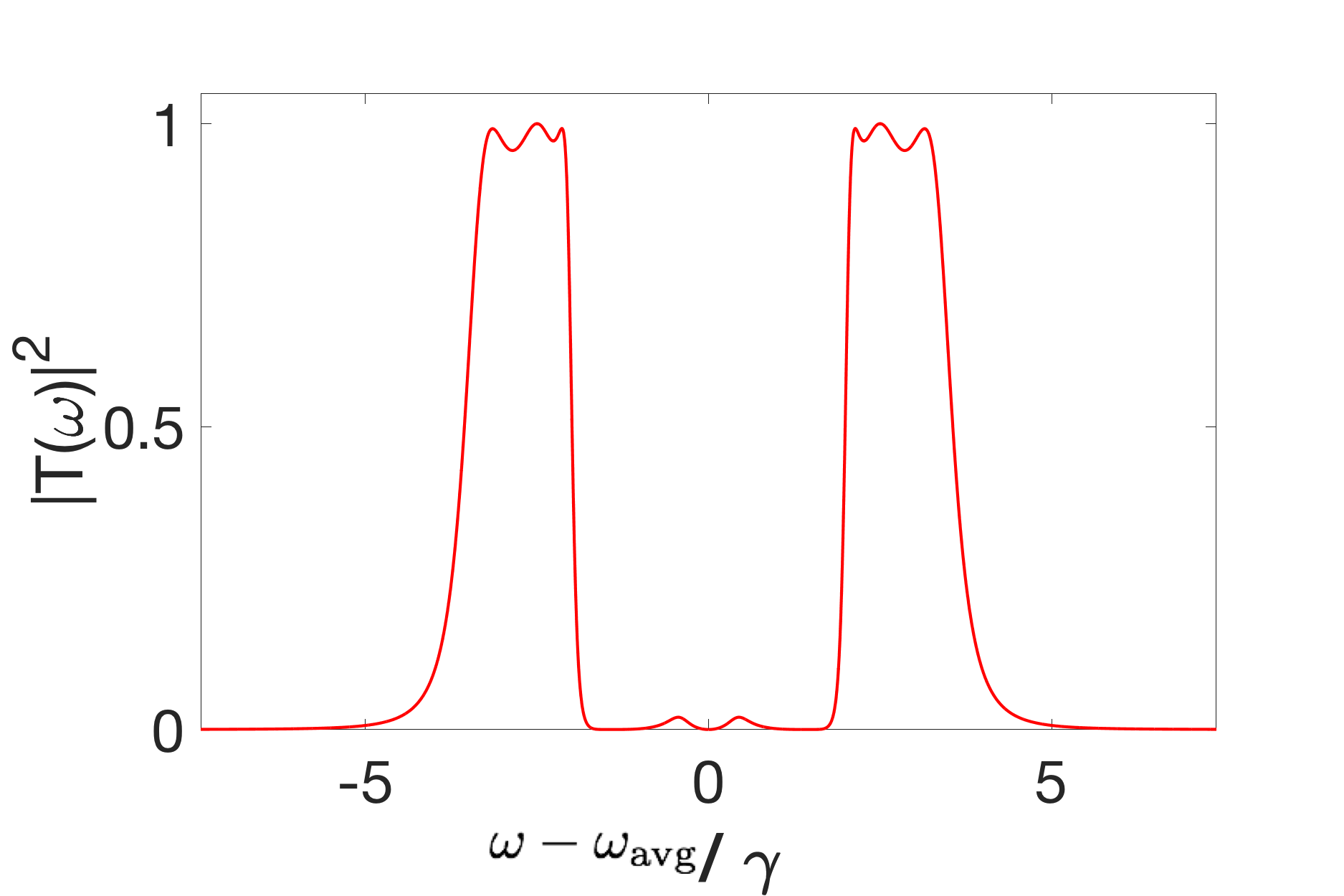
Figure 3.24: Transmission probability for a hybrid network consisting of $3$ manifolds in series, the first with $2$ discrete states and the second and third with $3$ discrete states, with balanced decays and uniform coupling ${g=\frac{\sqrt{\gamma\Gamma}}{2}}$ (the critical value for networks without detuning). Within the first manifold, the discrete states have frequency spacing $5\gamma$. Within the second and third manifolds, the discrete states are detuned by $\frac{5}{2}\gamma$, resulting in relative detuning between the manifolds. Since the couplings are no longer tuned to the critical parameters for a detuned system, perfect transmission is only achieved at $6$ frequencies.

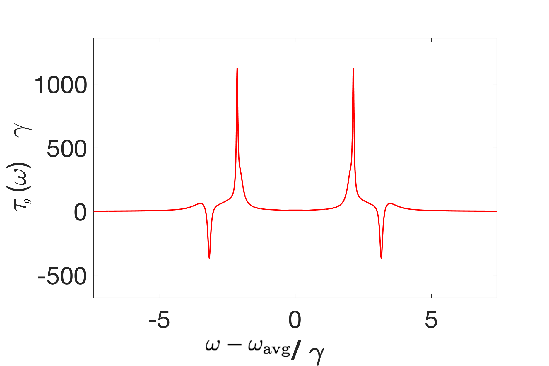
Figure 3.25: Group delay for a hybrid network consisting of $3$ manifolds in series, the first with $2$ discrete states and the second and third with $3$ discrete states, with balanced decays and uniform critical coupling.

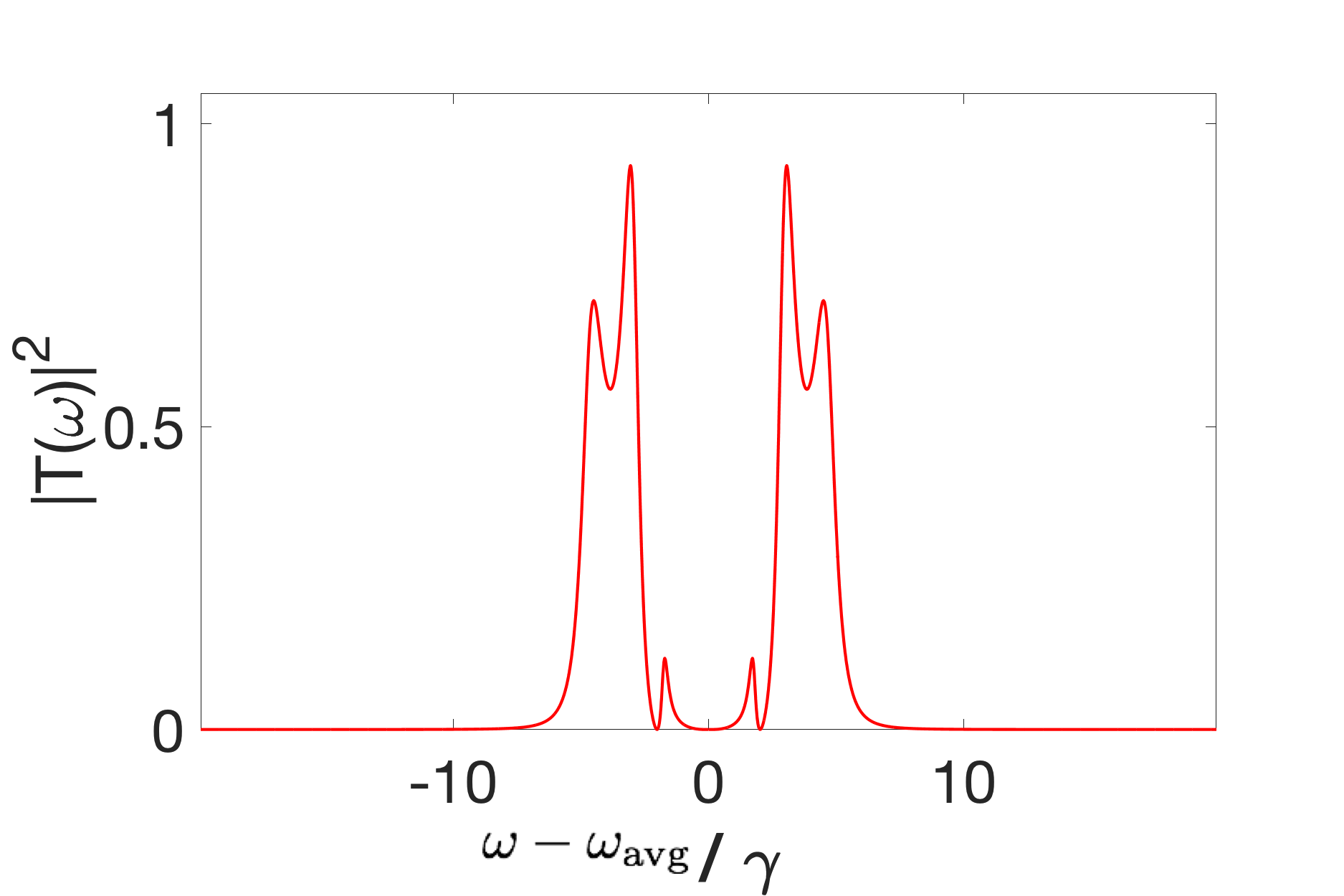
Figure 3.26: Transmission probability for a hybrid network consisting of $3$ manifolds in series, the first two with $2$ discrete states and the third with $3$ discrete states, with balanced decays ${\gamma=\Gamma}$ and uniform coupling ${g=\sqrt{\gamma\Gamma}}$. Within the first and second manifolds, the discrete states are spaced by ${\frac{5}{2}\gamma}$. Within the third manifold, the discrete states are spaced by $7\gamma$. Now no frequencies are perfectly transmitted, and finding couplings such that perfect transmission is achieved becomes less trivial.

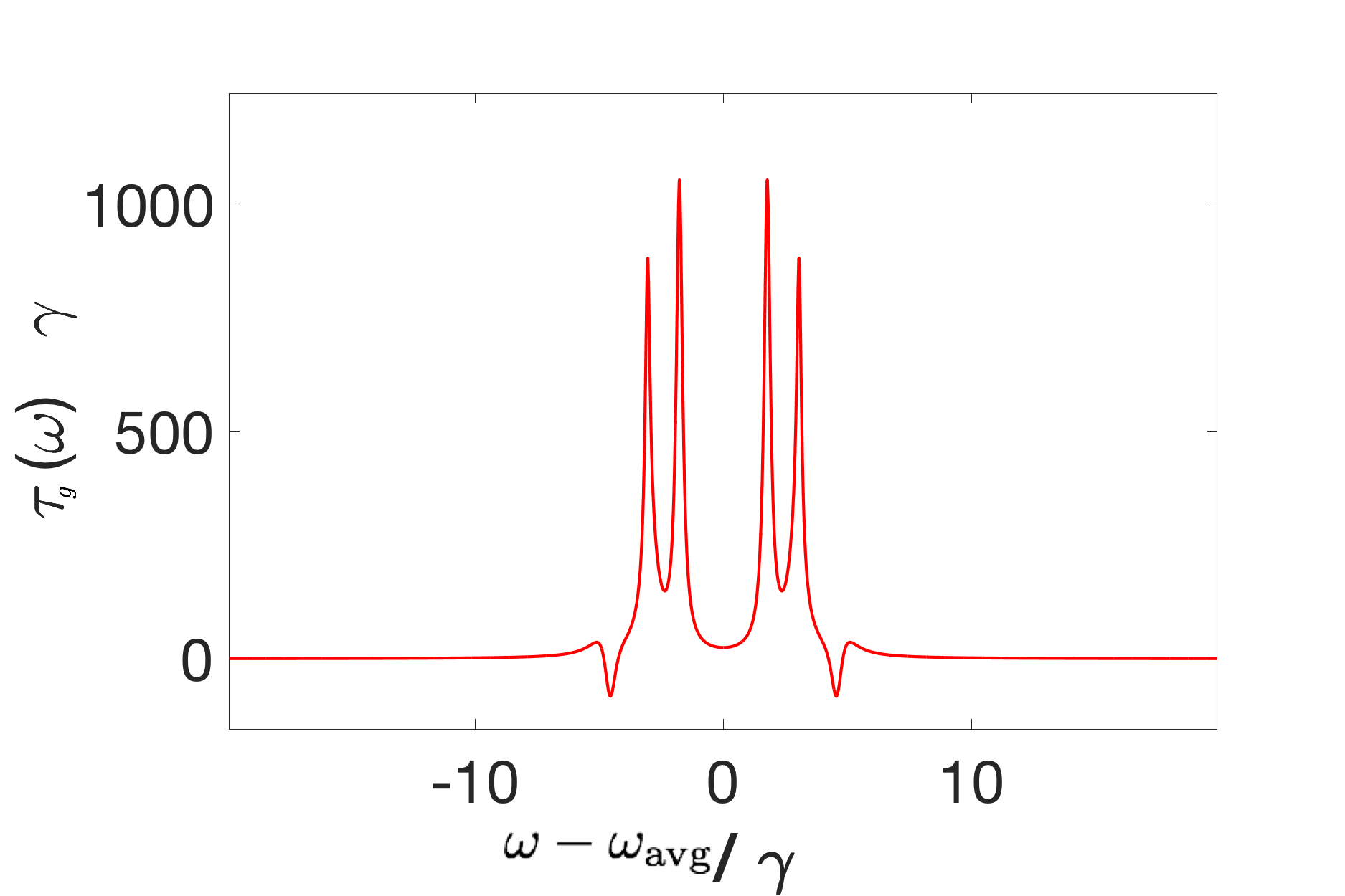
Figure 3.27: Group delay for a hybrid network consisting of $3$ manifolds in series, the first two with $2$ discrete states and the third with $3$ discrete states, with balanced decays ${\gamma=\Gamma}$ and uniform coupling ${g=\sqrt{\gamma\Gamma}}$, the transmission probability for which is shown in Fig. 3.26.

3.4 Other Networks

3.4.1 General Two-Sided Networks

We now begin to extrapolate from the above analyses to a larger class of two-sided networks. Both the series networks and hybrid networks we’ve discussed have the key property of asymptotic irrelevance of the causal ordering of discrete states in the strong coupling limit. This means that the asymptotically strong-coupling behavior of these networks is entirely described by fully parallel networks as in (3.19), and we can make several statements that will apply to any network that has the same behavior (that is, a network that resembles (3.19) in the strong coupling limit). From the structure of (3.19) alone, we can bound the total number of peaks and troughs of $|T(\omega)|^{2}$; we find there are at most $2N-1$ peaks and $2N-2$ troughs in the strong coupling limit and since the number of maxima never decreases with increasing $g$, we can extrapolate these bounds to weakly coupled systems as well. In transitioning from $2N-1$ peaks or constructive interference to $N$ peaks of perfect transmission, we observe a pair-wise merging of peaks (with one extra peak leftover when $N$ is odd). We also find that the number of dips of zero transmission (perfect reflection) is at most $\sum\limits_{k=1}^{M}(N_{k}-1)\leq N-1$ where the latter equality is only reached for a completely parallel network or in the strong coupling limit.

We suspect that the above argument for upper bounds applies more generally than just to the specific networks consisting of manifolds in series; that is, there is a large class of networks that reduce to a parallel description in the strong coupling limit. However, it is unproven! We cannot generalize from the above analysis to a fully arbitrary two-sided network as there also are networks with different topologies; for instance, we can consider networks with loops of discrete states that exist outside the main chain of manifolds that connect the two continua. Since it is not necessary for a photon to pass through the loop of discrete states to make it through the network, these networks behave differently in the strong coupling limit. We can make a further distinction between disconnected loops (dead-ends where photons have to back track) and connected loops (chains of manifolds that provide an alternate route to the output continua). It is possible that connected loop networks behave more like the loop-free networks discussed above in the strong-coupling limit, but with their specific loop-structure encoded in $T(\omega)$ in unexpected ways.

3.4.2 Additional Continua

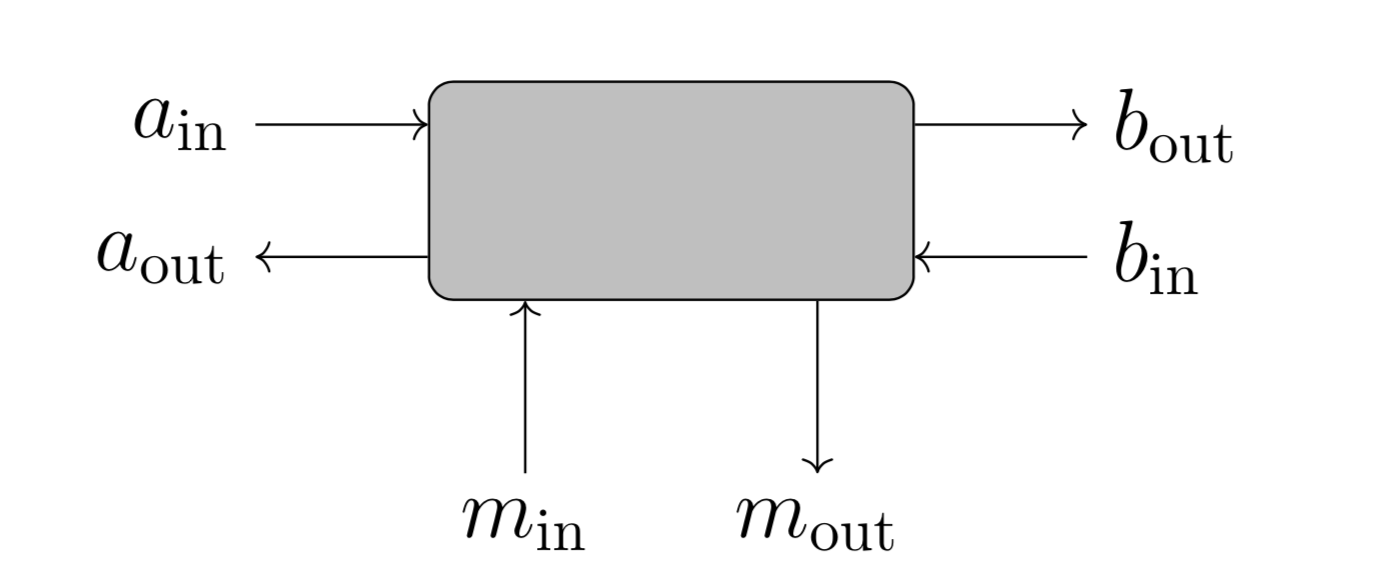
Figure 3.28: Input-output field operators for a black box network with one additional side channel. This will give rise to losses that make perfect transmission impossible, as well as dark counts if the side channel contains excitations (i.e. thermal).

We have thus far only considered quantum networks with two continnua, and have shown that perfect transmission through a general network structure is possible. We will briefly analyze more general multi-port quantum networks (Fig. 3.28) to illustrate how they lead to inefficiencies and dark counts.

Introducing a third continuum coupled to our network of discrete states at rates $\mu_{i}$, we rewrite (3.16) in the form

$$-i\Delta_{i}c_{i}(\omega)=-\sum\limits_{j}\,\left(\frac{\sqrt{\gamma_{i}\,\gamma_{j}}+\sqrt{\Gamma_{i}\,\Gamma_{j}}+\sqrt{\mu_{i}\,\mu_{j}}}{2}+ig_{i\,j}\right)c_{j}(\omega)$$

$$-\sqrt{\gamma_{i}}\,b_{in}(\omega)-\sqrt{\Gamma_{i}}\,a_{in}(\omega)-\sqrt{\mu_{i}}\,m_{in}(\omega),$$ (3.31)

where we have introduced a new input field annihilation operator $m_{in}(\omega)$ for the additional continuum (satisfying the canonical commutation relations), satisfying the same form of input-output relations as in (3.3)

$$m_{out}(\omega) =m_{in}(\omega)+\sum_{i}\,\sqrt{\mu_{i}}\,c_{i}(\omega).$$ (3.32)

When there are side channels and all decay rates in the system are homogenous ($\mu_{i}=\mu$, $\gamma_{i}=\gamma$, and $\Gamma_{i}=\Gamma$), it is impossible to achieve perfect transmission at any input frequency without adding additional excitations (active filtering). To see this, consider taking expectation values and imposing $m_{in}(\omega)\rightarrow 0$ over all frequencies. Flux conservation requires that, for a perfectly transmitted frequency $\omega^{\prime}$, we also have $m_{out}(\omega^{\prime})\rightarrow 0$. From (3.32), we see the only way to achieve this is for $\sum_{i}c_{i}(\omega^{\prime})\rightarrow 0$ but from (3.3), we see that this results in $a_{out}(\omega^{\prime})=a_{in}(\omega^{\prime})$ and $b_{out}(\omega^{\prime})=b_{in}(\omega^{\prime})$—the frequency $\omega^{\prime}$ is instead perfectly reflected by the system.

It is still possible that side channels with inhomogeneous coupling $\mu_{i}$ could yield a system that perfectly transmit some light at a frequency $\omega^{\prime}$ satisfying both conditions $a_{out}(\omega^{\prime})=a_{in}(\omega^{\prime})-\sum_{i}\,\sqrt{\gamma_{i}}c_{i}(\omega^{\prime})=0$ and $\sum_{i}\,\sqrt{\mu_{i}}c_{i}(\omega^{\prime})=0$. After all, the $c_{i}(\omega^{\prime})$ with resonant frequencies above and below $\omega^{\prime}$ generically differ in phase by $\pi$ and could in principle cancel out. However, this would require incredible fine-tuning of the system. For a uniformly inhomogeneous parallel network such as (3.23) with a side channel, we can easily see that this approach fails even in the low-loss limit near resonance (where it would be most likely to succeed): we find $m_{out}(\omega_{j})\approx\frac{2\mu_{j}}{\gamma_{j}+\Gamma_{j}}a_{in}(\omega_{j})$. In general, output channels outside your control lead to loss.

Similarly, we can determine from (3.4.2) and (3.32) that, in general, input channels outside your control lead to extra dark counts; photons that are in initially populated side channel can end up in the monitored continuum. If the side channel is at a finite temperature, there will be thermal photons that could populate the system. The probability of this vanishes for $k_{b}T\ll\hbar\omega_{i}\,\forall i$, but will generally be non-negligible for high-temperature systems. The specific contribution depends on the specific form of the full transfer matrix, which now will include a function $D_{m}(\omega)$ that governs the probability of thermal excitations in the side channel to end up in the monitored continuum.

Of course, the internal mode $b_{{\rm in}}$ may be occupied by thermal excitations as well, but the contribution to dark counts by these will depend strongly on the amplification mechanism. Furthermore, if only frequencies such that $|T(\omega_{i})|=1$ are amplified, we find that thermal excitations $b_{{\rm in}}$ do not contribute at all to dark counts as they always leak out of the system, ending up in the continuum mode $a_{{\rm out}}$ populated by reflected input photons.

3.5 Results

We have studied the behavior of quantum networks and have found that they provide a diverse structure of transmission functions for modeling the first stage of single-photon detectors: transmission of a single excitation from the input continuum, through the system, to a monitored output continuum. Inefficiencies and dark counts can be modeled through the incorporation of additional continua (side channels). While we do not find fundamental limits to transmission efficiency, spectral bandwidth, or frequency-dependent group delay across all the studied networks (series, parallel, and hybrid), we do observe that some networks are better suited to certain applications than others, as we will now discuss.

Perfect Transmission.— Often the most important metric for a photodetector is photo detection efficiency, which for a quantum network is tantamount to ensuring $|T(\omega_{i})|=1$ is achieved for some frequency or frequencies $\omega_{i}$. The main conclusions of this chapter are as follows:

• Ensuring the decay rates to the input and output continua are balanced ($\gamma=\Gamma$) guarantees perfect transmission for at least one frequency in almost all quantum networks without loops, side channels, and detunings [including all not covered by (ii)].

• Ensuring the couplings between manifolds are uniform and critical ($g=\frac{\sqrt{\gamma\Gamma}}{2}$) guarantees perfect transmission for at least one frequency in almost all quantum networks without loops, side channels, and detunings [including all not covered by (i)].

• For an arbitrarily detuned quantum network without loops and side channels, we are always able to find conditions for the couplings and decay rates such that perfect transmission occurs for at least one frequency.

That finding conditions such that perfect transmission $|T(\omega_{i})|=1$ is always possible indicates that perfect photo detection is possible in a wide variety of physical systems.

If one additionally wants a broadened transmission spectrum at a particular perfectly transmitted frequency—so that a broad range of frequencies is detected almost perfectly—we similarly find a variety of ways to accomplish it. One way is to use a parallel network distributed over a small range of states. However, this will result in a number of dark states which will not be detected at all. Instead, it is better to use a series network that meets both the critical coupling and balanced decay conditions, resulting in a maximally broadened on resonance transmission function as seen in Fig. 3.18.

Spectral Bandwidth.— We do not find fundamental limits to the minimum or maximum bandwidth of a network $\tilde{\Gamma}$ (or, conversely, to the interaction time between a network and incident light $\tilde{\Gamma}^{-1}$), but that it is generally proportional to the decay rates to both the input and monitored continua ($\tilde{\Gamma}\propto\frac{\gamma\Gamma}{\gamma+\Gamma}$, here assumed to be homogenous across states). We also find that some network structures are more suited to high-bandwidth applications than others; for networks with equivalent decay rates, we generally find that $\tilde{\Gamma}_{\rm series}\leq\tilde{\Gamma}_{\rm simple}\leq\tilde{\Gamma}_{\rm parallel}$. For a series network, equality with the upper limit of $\tilde{\Gamma}_{\rm simple}=\frac{2\gamma\Gamma}{\gamma+\Gamma}$ is reached only in the strong-coupling limit, and the lower limit ($\tilde{\Gamma}=0$) corresponds to a completely de-coupled or infinitely-detuned network (so that a photon can never pass through). For a parallel network, the bandwidth is always given $\tilde{\Gamma}_{\rm parallel}=\sum_{i}=\frac{2\gamma_{i}\Gamma_{i}}{\gamma_{i}+\Gamma_{i}}$ regardless of detuning, so the lower limit simply corresponds to a single discrete state (reproducing the simple model). Unlike both series and hybrid networks where the spectral bandwidth decreases with detuning, the spectral bandwidth of a parallel network is independent of detuning. This makes parallel networks the better candidate for implementation of broadband single-photon detection where the frequencies that need to be detected are distinct (so that spectral hole-burning is a non-issue).

Considering hybrid networks, we find that their bandwidths are bounded above and below by parallel and series networks, respectively; given a series network with the same coupling strengths and manifold-number, and a parralel network with the same manifold resonance structure and decay rates, the bandwidth of a Hybrid network is bounded $\tilde{\Gamma}_{\rm series}\leq\tilde{\Gamma}_{\rm hybrid}\leq\tilde{\Gamma}_{\rm parallel}$. The upper limit for a hybrid network is approached only in the limit of strong coupling, and the lower limit is approached when there is only a single discrete state in each manifold.

Group Delay.— The maximum magnitude of frequency-dependent group delay $\tau_{g}(\omega)$ increases with both the couplings between discrete states and the density of oscillations in the transmission function $T(\omega)$. In particular, the bounded-box structure of a uniformly coupled series networks yields large delays near $\omega=\pm 2g$. We observe that a negative group delay may occur for series networks with relative detuning between the discrete states. (For more on negative group delay, see Ref. [170].) For general networks, the group delay can vary immensely over the range of frequencies where $|T(\omega)|^{2}$ is non-negligible, with the effect being strongest for hybrid networks (where the resonance structures can be most dense). This means we can expect dispersion effects to be substantial in many photo detection platforms. For applications such as frequency discriminating delay-lines, we may expect hybrid networks to be the best performing candidate as they allow for the finest control of group delay structure.

Tradeoffs.— For an arbitrary series or hybrid network with arbitrary decay rates, perfect transmission requires a particular choice of the couplings. This critical value is generically of order $\sqrt{\frac{\gamma\Gamma}{2}}$. However, the spectral bandwidth is maximized when $g\gg\sqrt{\frac{\gamma\Gamma}{2}}$. Furthermore, the magnitude and location of the maximum group delays depends strongly on the coupling $g$ (and especially so in the high-$N$ limit). So for series and hybrid networks, there is a clear tradeoff between efficient transmission and the spectral bandwidth (which saturates in the high-$g$ limit), with the group delay changing as well. We contrast this with the case of parallel networks where the three quantities are completely independent: perfect detection requires balanced decays ($\gamma=\Gamma$), the bandwidth can be directly scaled by scaling both decay rates together, and the frequency-dependent group delay $\tau_{g}(\omega)$ alone depends on the detuning between discrete states, which is an independent quantity. So for photodetectors where all three quantities must be determinable independently, parallel networks are the best choice. The exception to this are situations where a negative group delay is required, which parallel networks never exhibit. Then the use of a hybrid or series network is unavoidable, as are their accompanying tradeoffs.

Final Remarks.— We have studied a variety of quantum networks to uncover tradeoffs and limits fundamental to single-photon detection that may arise in the first step of photo detection (transmission). The spectral bandwidth is the only main quantity of interest where there appear to be fundamental limits for particular classes of networks (parallel, series, and hybrid), but even these scale with the relevant decay rates for the networks. Given the freedom to adjust coupling strengths and decay rates, arbitrary group delay, transmission efficiency, and spectral bandwidth are attainable for any network so long as they are attained individually (together there may be tradeoffs for series and hybrid networks).

We do not find fundamental limitations to dark counts and losses in this analysis of transmission: in general uncontrolled input channels lead to dark counts and uncontrolled output channels lead to loss. These can always be mitigated by cooling the system ($k_{b}T\ll\hbar\omega_{i}\,\forall i$) and reducing coupling to side channels ($\mu_{i},\,\nu_{i}\ll\gamma_{i}+\Gamma_{i}\,\forall i$). These side channels can be as simple as material absorption, where a photon cab be absorbed by the material of the photodetector and contributes to a heating process and where the material of the photodetector acts as a thermal bath, generating potential dark counts.

Other sources of noise, such as from signal amplification (for more on this specifically, see Ref. [5]), classical parameter fluctuations, as well as the noise inherent in a non-ideal quantum measurement (as described by an arbitrary photo detection POVM) can also be included in our model to give a fully quantum description of the entire single-photon detection process, as will be done in the coming sections.

3.6 An Additional Toy Model POVM

In this chapter, we have not yet discussed in detail what happens to the excitation after it ends up in the output mode $b_{{\rm out}}$, except that it can give rise to a macroscopic photodetector click. Following Ref. [143], we can construct an extremely simplified POVM from $T(\omega)$ by assuming any excitation in the output continuum will lead to a click (that is, that the continuum is monitored). This single-step POVM will not be realistic, but it has pedagogical value in highlighting the role of $T(\omega)$ in our work.

Assume that we finalize the photo detection process by ascertaining at some time $t$ whether an excitation is indeed in the continuum $b_{{\rm out}}$ and also that the amplification is ideal and lossless so that, if a photon makes it to the monitored continuum, it will be detected. We can then define normalized filtered photon states (following Ref. [143])

$$\left|T\,\phi_{t}\right\rangle=\frac{1}{\sqrt{\pi\,\tilde{\Gamma}}}\int_{0}^{\infty}\,d\omega\,T^{*}(\omega)\,e^{i\,\omega\,t}\,\hat{a}^{\dagger}(\omega)\,\left|\textnormal{vac}\right\rangle.$$ (3.33)

From the quantum jump method [171, 89], we know that a quantum jump from the final manifold of discrete states to the monitored output continuum will occur in an infinitesimal time $dt$ with conditional probability $\frac{\tilde{\Gamma}\,dt}{2}$. We then infer the POVM element for detecting a photon at a particular time $t$ after the photodetector has been on for a time $dt$

$$\hat{\Pi}_{t}=\frac{\tilde{\Gamma}\,dt}{2}\,\left|T\,\phi_{t}\right\rangle\left\langle T\,\phi_{t}\right|.$$ (3.34)

(To reiterate, here $t$ refers to a possible time of detection analogous to the time $T$ from the previous chapter, and does not refer to the time evolution of the input state.) The probability of getting a click for a normalized input photon $\hat{\rho}$ is $\textnormal{Tr}\left(\hat{\Pi}_{t}\hat{\rho}\right)\leq 1$. So the input state that will be detected with maximum probability is $\hat{\rho}=\left|T\,\phi_{t}\right\rangle\left\langle T\,\phi_{t}\right|$, yielding an infinitesimal probability of detection of $\frac{\tilde{\Gamma}\,dt}{2}$. This is because this assumes that the detection events at times separated by a time $dt$ correspond to different measurement outcomes which is highly idealized; any realistic photo detection outcome corresponds to detection within an integrated time-window. Nonetheless, (3.34) provides a POVM description of a continuous measurement process, and can be used to construct a partition of unity.

To take a finite time-window into account, we consider a time-integrated POVM element $\hat{\Pi}_{\tau}$, where a click corresponds to an excitation entering the final output continuum sometime between $t=T_{0}$ when we first turn on the detector and $t=T_{0}+\tau$. Then the time-integrated POVM element is

$$\hat{\Pi}_{\tau}=\int_{T_{0}}^{T_{0}+\tau}\,dt\,\frac{\tilde{\Gamma}}{2}\,\left|T\,\phi_{t}\right\rangle\left\langle T\,\phi_{t}\right|$$

$$\approx\int_{-\infty}^{\infty}\,d\omega\,|T(\omega)|^{2}\left|\omega\right\rangle\left\langle\omega\right|\,\,\,\,\,\,(\tau\gg\tilde{\Gamma}^{-1})$$ (3.35)

where, for $\tau\rightarrow\infty$, the projectors $\left|\omega\right\rangle\left\langle\omega\right|$ are truly monochromatic because no timing information is obtained. With the time-integrated form in (3.6), we can see that the conditions for perfect transmission discussed above correspond to perfect detection in the limit of $\tau\gg\tilde{\Gamma}^{-1}$ as we used previously in (3.6). Physically, a non-infinitesimal integration time $\tau$ means a photon incident on the photodetector at a time $t=-\tau$ has had sufficient time to propagate through the network before we end the integration at time $t=0$ and check whether there has been a click. This is in agreement with our observation that, for the simple model in (3.8), $\tau_{g}(\omega_{0})=\tilde{\Gamma}^{-1}$: simply, we must at least allow enough time for an on-resonance photon to travel through the network (interact with the device) to achieve perfect detection of a monochromatic on-resonance photon. (3.6) is also illustrative of what the POVM element represents: the information a detector click reveals about what led up to it.

We can also use (3.6) to construct the POVM element for not getting a click in the finite time $\tau$, which is simply $\hat{\Pi}_{0}=\hat{1}-\hat{\Pi}_{\tau}$, such that the full POVM $\{\hat{\Pi}_{0},\,\hat{\Pi}_{\tau}\}$ forms a partition of unity for the relevant Hilbert space; that is, the Hilbert space spanned by single-photon states and the vacuum. (See Ref. [98] for inclusion of general photon Fock states in the photo detection POVM.) This POVM corresponds to a photodetector that is reset after each integration time $\tau$. Similarly, one can divide up the the full detection window into $N$ time intervals $\tau_{i}$ without resetting the device in between so that the full POVM is $\{\hat{\Pi}_{0},\,\hat{\Pi}_{\tau_{i}}\}_{i=1...N}$, reproducing a continuous measurement POVM in the limit $\tau_{i}\rightarrow 0$. In this case, the measurement outcomes are not orthogonal [143]; even if we know a photon is incident at a definite time $t^{\prime}$ we cannot predict with certainty when it will be detected.

Chapter 4 Amplification

In this chapter, we show that detection of single photons is not subject to the fundamental limitations that accompany quantum linear amplification of bosonic mode amplitudes, even though a photodetector does amplify a few-photon input signal to a macroscopic output signal. Alternative limits are derived for nonlinear photon-number amplification schemes with optimistic implications for single-photon detection. Four commutator-preserving transformations are presented: one idealized (which is optimal) and three more realistic (less than optimal). Our description makes clear that nonlinear amplification takes place, in general, at a different frequency $\omega^{\prime}$ than the frequency $\omega$ of the input photons. This can be exploited to suppress thermal noise and dark counts past what is possible with linear amplification up to a fundamental limit imposed by nonlinear amplification into a single bosonic mode.

4.1 Quantum amplification and noise

The fundamental relations between quantum noise and quantum amplification are most straightforwardly derived in the Heisenberg picture. Thus, the standard way [172] to describe linear phase-preserving quantum amplification of a bosonic mode amplitude $a$ is through Caves’ relation for the annihilation operator $\hat{a}$,

$$\hat{a}_{{\rm out}}=\sqrt{G}\hat{a}_{{\rm in}}+\sqrt{G-1}\hat{b}^{\dagger}_{{\rm in}},$$ (4.1)

where $\hat{b}^{\dagger}$ is the creation operator corresponding to an independent auxiliary bosonic mode $b$. Here the input field amplitude of mode $a$ is amplified by a factor of $\sqrt{G}$, but there is a cost: extra noise arising from the additional mode $b$. If this mode contains (thermal) excitations, mode $a$ after amplification will contain excitations, too, and their number is multiplied by $G-1$. Even if mode $b$ is in the vacuum state, it still adds noise [172]. It is clear that this extra noise is due to the additional creation operator term proportional to $\sqrt{G-1}$ in Eq. (4.1), but since that term is necessary so as to preserve the standard bosonic commutation relation $[\hat{a}_{{\rm out}},\hat{a}^{\dagger}_{{\rm out}}]=\mathds{1}$ this tradeoff between linear amplification and added noise is fundamental. Indeed, phase-preserving linear amplification in proposed number resolving platforms using superconducting qubits have noise bounded by the Caves limit [173, 52] and similar bounds are found for linear amplification used in quantum circuits [174].

Recently, there has been some effort to describe all parts of the photodetection process, including amplification [175], fully quantum mechanically [176, 26, 98, 24]. One conclusion that may be drawn from that research is that there is no severe amplification-driven tradeoff between efficiency and (thermally induced) dark counts. In particular, even though a few-photon signal must be amplified to a macroscopic level [forcing us to consider $G\gg 1$], thermal fluctuations in internal detector modes apparently do not get amplified by the same factor of $G$. Experiments [22, 23] on superconducting nanowires demonstrate that over a wide range of detected wavelengths dark count rates can indeed be extremely low (on the order of one dark count per day). How can we reconcile these results with that of the previous paragraph?

The answer, as we will show, is that amplification is not necessarily linear. That is, in the Heisenberg picture, the transformation of the bosonic annihilation operator can be nonlinear while still preserving the bosonic commutation relation. And, perhaps surprisingly, that way of amplifying can decrease the amount of noise added. Previous models of nonlinear amplification were developed in a different context, that of amplifying superpositions of different number states [177, 178, 179, 180, 181, 182]. The relevant figure-of-merit there was the signal to noise ratio of the output relative to that of the input, and noise from the auxiliary modes was ignored. Here, in contrast, we are interested exclusively in the noise in the output and especially in the contributions arising from thermal fluctuations in the auxiliary modes, as functions of the gain factor $G$. In order to explore this issue, we construct physical transformations that implement nonlinear amplification satisfying the correct mathematical requirements which, to the authors’ knowledge, have not appeared in the literature.

4.2 Nonlinear amplification

The idea is that for detecting single photons it is sufficient to have an output field whose total number of excitations is given by $N_{\rm out}=N_{\rm in}+Gn_{a}$ with $n_{a}$ the number of input photons we would like to detect, and $N_{\rm in}$ the (fluctuating) number of excitations present in the output mode prior to amplification, which is itself not amplified. A physically allowed but highly idealized unitary transformation that accomplishes this is easiest written down in the Schrödinger picture as

$$\left|n\right\rangle_{a}\left|M\right\rangle_{1}\left|N\right\rangle_{2}\longmapsto\left|n\right\rangle_{a}\left|M-Gn\right\rangle_{1}\left|N+Gn\right\rangle_{2}.$$ (4.2)

This is valid for any number $n$ of input photons, even though in practice we will be interested mainly in small values of $n$, say, $n=0,1,2$).

All states here are number (Fock) states of bosonic modes and as written this transformation is superposition-preserving. The transformation involves two energy reservoirs: energy is transferred from the first reservoir to the second with the amount of energy transferred determined by the number $n$ of input photons in mode $a$ (with nothing happening at all when $n=0$). The assumption is that excitations of the two reservoirs have identical energies, $\hbar\omega^{\prime}$, such that energy is conserved. The input mode can have any frequency $\omega$. The second reservoir ideally starts out with $N=0$ excitations—corresponding to the zero temperature limit—such that in the end it would contain exactly $Gn$ excitations if the input field contained $n$ photons. Clearly, this ideal transformation would represent perfect (noiseless) amplification of a photon number state (and $G$ will have to be an integer for this to work).

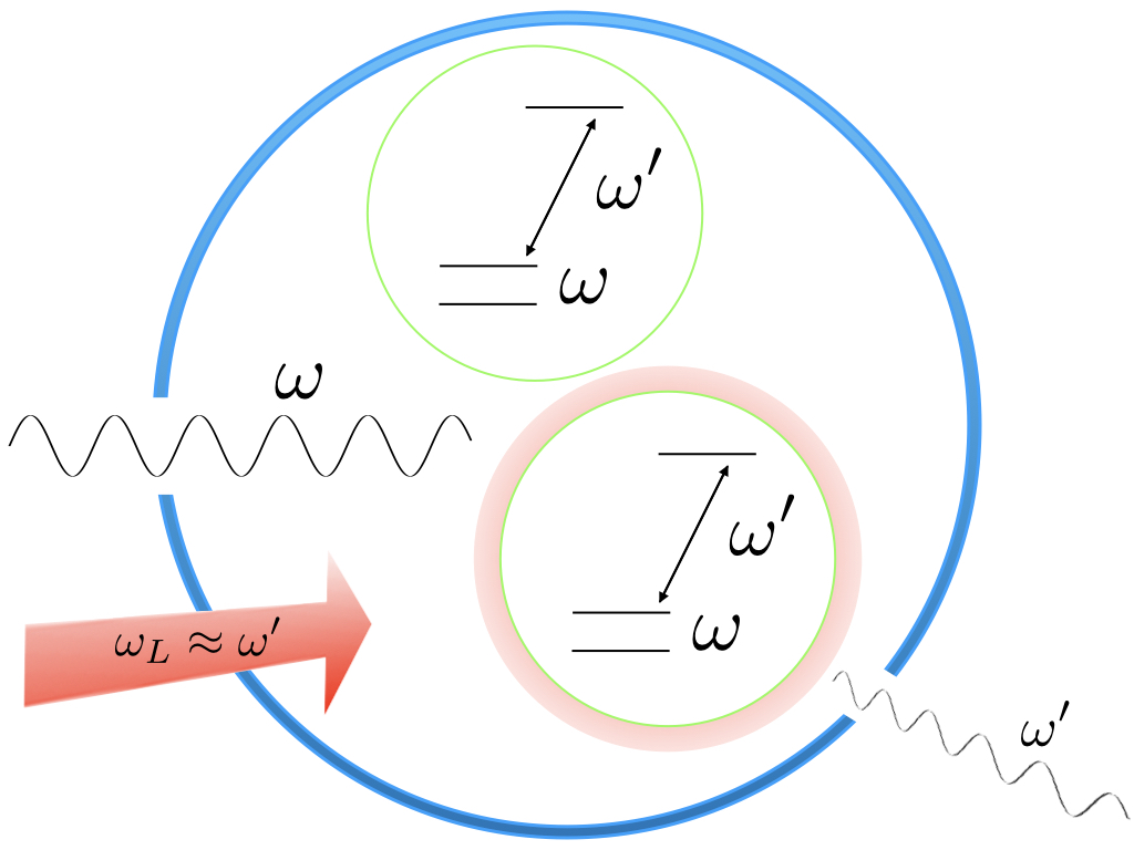
Figure 4.1: An input photon with frequency $\omega$ undergoes amplification into a macroscopic signal via electron-shelving [31, 183, 184]: when an on-resonance photon is absorbed, an atom (modeled here as a three-level system) enters the first excited state. This is followed by a laser beam tuned to the second transition frequency ${\omega_{L}\approx\omega}^{\prime}$, which induces fluorescence. If there are multiple input photons, they are absorbed by multiple atoms and the fluorescence signal is increased proportionally. The number of fluorescence modes may be reduced by placing a high-Q cavity around the atom so that amplification moves towards the ideal transformation given in Eq. 4.2.

Now we wish to describe this ideal process in the Heisenberg picture so as to make a direct comparison with Eq. (4.1). In that picture, the ideal transformation that is linear in the number operator for the excitations in the second reservoir should be

$$\hat{b}^{\dagger}_{\rm out}\hat{b}_{\rm out}=\hat{b}^{\dagger}_{\rm in}\hat{b}_{\rm in}+G\hat{a}^{\dagger}_{\rm in}\hat{a}_{\rm in}.$$ (4.3)

We are now going to do three things: (A) we will construct expressions for $\hat{b}^{\dagger}_{\rm out}$ and $\hat{b}_{\rm out}$ such that Eq. (4.3) is reproduced and such that their commutator $[\hat{b}^{\dagger}_{\rm out},\hat{b}_{\rm out}]=\mathds{1}$; (B) we will add non-ideal features that make the model more realistic, and (C) we will include fluctuations in the initial number of excitations in the $b$ mode and calculate the signal-to-noise ratio (SNR) for the final number of excitations in the $b$ mode, both for the ideal limit and the more realistic models. A comparison with linear amplification will then show how nonlinear amplification improves upon the former.

To start with part of task (B), we adjust the idealized Schrödinger picture to get rid of two features that make the process in Eq. (4.2) obviously inapplicable to real detectors, but such that the Heisenberg picture Eq. (4.3) is still valid. First note that the $n$ photons in the process in Eq. (4.2) are not destroyed, whereas in a standard detector they are. We fix that by introducing another quantum system $S$ with a continuum of energies $E$ that can absorb the energy $n\hbar\omega$ of the $n$ photons. This modifies Eq. (4.2) by adding a step (potentially at a later time)

$$\left|n\right\rangle_{a}\left|E\right\rangle_{S}\longmapsto\left|0\right\rangle_{a}\left|E+n\hbar\omega\right\rangle_{S}.$$ (4.4)

Since this extra step does not affect the state of reservoir 2, the crucial expression Eq. (4.3) is unchanged when the continuum of energies absorbing the energy is traced over. The second change concerns phase: in the Schrödinger picture we can insert random phase factors $\exp(i\phi^{\mbox{$\clubsuit$}})$ on the right-hand side of Eq. (4.2). Critically, this is not a global phase but a local phase factor, that will be different even for the same Fock state. Thus, the amplification process destroys superpositions of different number states (e.g., coherent states will not be coherently amplified) and the process is now also irreversible (as any amplification process in a real detector is). It destroys any entanglement between the different modes as well.

For task (A) we would like to use the polar decompositions of the creation and annihilation operators. That is, in analogy to the polar decomposition of a complex number, $z=\exp(i\phi)\sqrt{|z|^{2}}$, we would like to write

$$\hat{b}_{{\rm out}} =\hat{S}\,\sqrt{(\hat{b}^{\dagger}\hat{b})_{{\rm in}}+G(\hat{a}^{\dagger}\hat{a})_{{\rm in}}},$$ (4.5)

where $\hat{S}$ is a unitary operator which could be written in the suggestive form $\exp(i\hat{\phi})$ for some hermitian operator $\hat{\phi}$. In a finite-dimensional Hilbert space of dimension $s+1$ there is no problem defining $\hat{S}$: it is a shift operator that acts on number states $\left|N\right\rangle$ of the bosonic mode as

$$\hat{S}\left|N\right\rangle=e^{i\phi^{\mbox{$\clubsuit$}}}\left|N-1\right\rangle\,\,\,{\rm for}\,\,s\geq N>0,$$ (4.6)

with $\hat{S}\left|0\right\rangle=\left|s\right\rangle$ and $\phi^{\mbox{$\clubsuit$}}$ the random phase we introduced earlier. Since Fock space is infinite-dimensional, we use the Pegg-Barnett trick [185] of truncating the Hilbert space at a high excitation number $s$ and only in the end (when calculating physical quantities) taking the limit $s\rightarrow\infty$. It is easy to verify that the relation Eq. (4.5) yields the commutator $[\hat{b}_{{\rm out}},\hat{b}^{\dagger}_{{\rm out}}]=\mathds{1}_{{\rm in}}-(s+1)\left|s\right\rangle\left\langle s\right|$, in which the extra Pegg-Barnett term won’t contribute to any physical quantity, while ensuring a traceless commutator, necessary in finite dimensions.

Construction of Hamiltonians that implement nonlinear photon number amplification was done elsewhere (see [180, 182]), but they are far more complicated than the Hamiltonians implementing linear amplification; in the interaction picture phase-preserving linear amplification is implemented with the simple interaction Hamiltonian

$$\hat{H}=i\hbar\kappa(\hat{a}\hat{b}-\hat{a}^{\dagger}\hat{b}^{\dagger})$$ (4.7)

which amplifies via two-mode quadrature squeezing (as introduced in Ref. [186]) with a (non-integer) time-dependent gain factor $G=\cosh(\kappa t)$ with $\kappa$ the coupling strength and $t$ the interaction time [187]. In contrast, an interaction Hamiltonian implementing nonlinear amplification even for a modest gain of $G=5$ has $40$ terms (fewer terms for smaller $G$, more terms for larger $G$) [182]. Since we are only interested in the output signal and not the details of the evolution of other operators, we will not construct a system Hamiltonian; indeed, the same transformation on the output signal could be given by different Hamiltonians corresponding to different physical implementations of photon number amplification that give the same overall gain factor.

The nonlinear expression Eq. (4.5) does not seem to have appeared in the large literature on bosonic amplification (for a review, see, e.g., [52]). [177, 178, 179] did discuss photon-number amplifiers (especially in the high-photon number limit) decades ago, but no attempt was made there to find commutator-preserving operator equations.

4.3 More realistic models for amplification

Continuing with task (B), in a more realistic description the reservoirs consist of many modes. So, instead of having just one bosonic output mode $b$ we really should describe many output reservoir modes. For example, we may have $G$ modes $b_{k}$ [recall that for non-linear amplification $G$ must be an integer] each one of which satisfies

$$\hat{b}_{k\,{\rm out}} =\hat{S}_{k}\,\sqrt{(\hat{b}^{\dagger}\hat{b})_{k\,{\rm in}}+(\hat{a}^{\dagger}\hat{a})_{{\rm in}}},\,\,\,\,\,k=1\ldots G.$$ (4.8)

Here the macroscopic signal monitored and analyzed consists of the sum of all detected excitations (since each mode by itself contains just a microscopic number of excitations we cannot simply assume to be able to count those individual numbers: then we would not need amplification at all!). That is, we consider as our macroscopic output signal

$$\hat{I}_{{\rm out}}=\sum_{k=1}^{G}(\hat{b}^{\dagger}\hat{b})_{k\,{\rm out}}=\sum_{k=1}^{G}(\hat{b}^{\dagger}\hat{b})_{k\,{\rm in}}+G(\hat{a}^{\dagger}\hat{a})_{{\rm in}}.$$ (4.9)

Another extension is to “avalanche” photodetection where one small-scale amplification event triggers the next and the process repeats, giving rise to a macroscopic signal. Iterating the transformation Eq. (4.3) of single mode amplification $N$ times with a gain factor $g$ in each step gives a total gain factor $G=g^{N}$ and an input-output relation

$$(\hat{b}^{\dagger}\hat{b})_{\rm N\,out}=\sum_{k=1}^{N}g^{N-k}(\hat{b}^{\dagger}\hat{b})_{k\,{\rm in}}+G(\hat{a}^{\dagger}\hat{a})_{{\rm in}}$$ (4.10)

where mode $\hat{b}_{k}$ here contains the output of the $k$th amplification step, and the last mode $b_{N}$ contains the signal.

Another extension, relevant for $n>1$, describes multiplexing: the idea is that $n$ photons are most conveniently detected by $n$ detectors that each detect one (and only one) photon, along the lines of [188, 189]. We will not describe this model in any detail, except to state that amplification would in that case be described by $Gn$ modes, each containing exactly one extra excitation.

Lastly, we combine both multi-mode and multi-step extensions above by repeating the process in Eqs. (4.8) and (4.9) of amplification into several ($g$) modes $N$ times, again with a total gain factor defined $G=g^{n}$ and an input-output relation for the macroscopic signal

(4.11)

$$\hat{I}_{{\rm out}}=\sum_{k_{N}=1}^{G}(\hat{b}^{\dagger}\hat{b})_{k_{N}\,{\rm out}}=\sum\limits_{n=1}^{N}\sum\limits_{k_{n}=1}^{g^{n}}(\hat{b}^{\dagger}\hat{b})_{k_{n}\,{\rm in}}+G(\hat{a}^{\dagger}\hat{a})_{{\rm in}}$$

where the mode $\hat{b}_{k_{n}}$ is the $k_{n}$th mode in the $n$th step.

Note that in our nonlinear amplification models the amplified signal ends up in a different bosonic mode or modes: indeed, a photodetector typically converts the input signal (light) to an output signal of a physically different type, e.g., electron-hole pairs (which may sometimes be approximated as composite bosons; see also [190, 191, 192, 193]).

4.4 Number fluctuations

We turn to task (C) and calculate the noise in photon number introduced by the amplification process and by the coupling to reservoirs. For the reservoir we monitor, we write

$$\left\langle(\hat{b}^{\dagger}\hat{b})_{\rm{in}}\right\rangle=\overline{n}_{b};\,\left\langle(\hat{b}^{\dagger}\hat{b})^{2}_{\rm{in}}\right\rangle=\overline{n}^{2}_{b}+\Delta n_{b}^{2}$$ (4.12)

and make no further assumptions about its initial state.

We assume that there is some (unknown) number of photons in the input mode $a$ that we want to measure. We thus consider input states that are diagonal in the photon number basis, with some nonzero photon number fluctuations $\Delta n_{a}$. (Thanks to the randomized phase assumption we can use this assumption without loss of generality for our nonlinear models.) So, we write

$$\left\langle(\hat{a}^{\dagger}\hat{a})_{\rm{in}}\right\rangle=\overline{n}_{a};\,\left\langle(\hat{a}^{\dagger}\hat{a})^{2}_{\rm{in}}\right\rangle=\overline{n}^{2}_{a}+\Delta n_{a}^{2}.$$ (4.13)

In the following we always assume the initial states of modes $a$ and $b$ to be independent, such that

$$\left\langle f(\hat{a},\hat{a}^{\dagger})g(\hat{b},\hat{b}^{\dagger})\right\rangle=\left\langle f(\hat{a},\hat{a}^{\dagger})\right\rangle\left\langle g(\hat{b},\hat{b}^{\dagger})\right\rangle$$ (4.14)

for any functions $f$ and $g$.

For linear phase-insensitive amplification Eq. (4.1), we find the following variance in the number of excitations in the amplified signal:

$$\sigma_{(\hat{a}^{\dagger}\hat{a})_{\rm out}}^{2} = G^{2}\Delta n_{a}^{2}+(G-1)^{2}\Delta n_{b}^{2}+$$ (4.15)

$$G(G-1)(2\overline{n}_{a}\,\overline{n}_{b}+\overline{n}_{a}+\overline{n}_{b}+1).$$

We observe that in addition to amplification of the thermal fluctuations in the auxiliary mode $b$ [the second term in Eq. (4.15)], even at zero temperature where $\Delta n_{b}^{2}=0$ there is inherent noise from the amplification process itself [the second line is strictly positive for $G>1$].

We should also consider linear phase-sensitive amplification [172], described by

$$\hat{a}_{{\rm out}}=\sqrt{G}\hat{a}_{{\rm in}}+\sqrt{G-1}\hat{a}^{\dagger}_{{\rm in}}.$$ (4.16)

Here, compared to Eq. (4.1) the $\hat{b}^{\dagger}$ term is replaced by the $\hat{a}^{\dagger}$ term, such that the commutator $[\hat{a}_{{\rm out}},\hat{a}^{\dagger}_{{\rm out}}]$ is still preserved. This gives a variance

$$\!\!\sigma_{(\hat{a}^{\dagger}\hat{a})_{\rm out}}^{2} = (6G(G-1)+1)\Delta n_{a}^{2}+$$ (4.17)

$$2G(G-1)(\overline{n}^{2}_{a}+\overline{n}_{a}+1).$$

There is again extra amplification noise for $G>1$ [the second line], much like what we found for phase-insensitive amplification.

We compare these two results for linear amplification to the result for the nonlinear amplification process described by Eq. (4.5). The variance in excitation number is

$$\sigma_{(\hat{b}^{\dagger}\hat{b})_{\rm out}}^{2} =\Delta n_{b}^{2}+G^{2}\Delta n^{2}_{a}.$$ (4.18)

Here the number fluctuations in the auxiliary mode are not amplified and there is no additional amplification noise either; if the input field is in a number state such that $\Delta n_{a}=0$, the gain factor $G$ will not effect the noise at all. This is a result of the reservoir and auxiliary mode being coupled conditionally on the presence of the input field; the transformation Eq. (4.2) always transfers exactly $Gn$ excitations to the auxiliary mode, leaving the noise in the auxiliary mode unchanged when $\Delta n_{a}=0$. In contrast, linear amplification never adds a definite number of excitations to the auxiliary mode because the input mode and the auxiliary mode are directly coupled; even at zero temperature there is inherent noise from the amplification of the auxiliary mode amplitude by a factor $\sqrt{G-1}$ [see Eq. (4.1)]. For linear amplification this is necessary so as to preserve the spectrum of the number operator [which non-linear amplification through Eq. (4.3) does by construction].

Already we are able to see that the scheme of amplification into a single mode is optimal; any transformation that would reduce the prefactor of $\Delta n_{b}^{2}$ in Eq. (4.18) below unity would fail to realize a well-behaved annihilation operator (for details, see again)!

For nonlinear amplification into many modes described by the more realistic model in Eqs. (4.8) and (4.9), we find

$$\sigma_{\hat{I}_{\rm out}}^{2} =G\Delta n_{b}^{2}+G^{2}\Delta n^{2}_{a},$$ (4.19)

where for simplicity we assumed all reservoir modes to be independent with the same number fluctuations and we have defined $\hat{I}_{\rm out}$ as the integrated signal in Eq. (4.11). This shows amplifying according to Eq. (4.8) is suboptimal; even though it still beats both linear amplification limits Eqs. (4.15) and (4.17) the noise in the reservoir modes is still amplified. Similarly, amplification using multiple fermionic degrees of freedom will be sub-optimal; a similar multi-mode description will be necessary.

Defining the total gain $g^{N}=G$ with $N$ the number of steps, we find for our multi-step models that

$$\sigma_{(\hat{b}^{\dagger}\hat{b})_{\rm out}}^{2}=\frac{G^{2}-1}{g^{2}-1}\Delta n^{2}_{b}+G^{2}\Delta n^{2}_{a}$$ (4.20)

for amplification of $g$ excitations into a single mode and

$$\sigma_{\hat{I}_{\rm out}}^{2}=G\frac{G-1}{g-1}\Delta n^{2}_{b}+G^{2}\Delta n^{2}_{a}$$ (4.21)

for amplification of a single excitation into $g$ modes. (Note Eqs. (4.20) and (4.21) reduce to Eqs. (4.18) and (4.19) for $g=G$.)

4.5 Signal-to-noise ratios

We can now write down explicit tradeoff relations between amplification and number fluctuations in terms of signal-to-noise ratios for all types of amplification discussed here, for the case where the number of input photons is fixed to be $n_{a}$ (and so $\Delta n_{a}=0$). Using the standard signal-to-noise ratio as the number of excitations in the amplified mode minus the background, divided by the standard deviation in the number of excitations, we get

$$\textnormal{SNR}_{{\rm PhaseInsensitive}} \leq \frac{G}{G-1}\frac{n_{a}}{\Delta n_{b}}$$ (4.22)

$$\textnormal{SNR}_{{\rm PhaseSensitive}} \leq \frac{2G-1}{\sqrt{2G(G-1)}}n_{a}$$ (4.23)

$$\textnormal{SNR}_{{\rm SingleMode}} = \frac{Gn_{a}}{\Delta n_{b}}$$ (4.24)

$$\textnormal{SNR}_{{\rm GModes}} = \frac{Gn_{a}}{\sqrt{G}\Delta n_{b}}=\frac{\sqrt{G}n_{a}}{\Delta n_{b}}.$$ (4.25)

The linear amplification mechanisms have increasingly worse signal-to-noise ratios as $G$ increases, albeit saturating in the limit $G\rightarrow\infty$. In contrast, the signal-to-noise ratios for the nonlinear amplification mechanisms improve with increasing $G$, with amplification into a single-mode performing best, with an improvement by a factor of $G$ over an unamplified signal. Amplification into $G$ modes performs worse than single mode amplification, showing an improvement over an unamplified signal by a factor of $\sqrt{G}$. In the large $G$ limit, this can be considered the well-known $1/\sqrt{G}$ reduction in the standard error; while there are $G$ noisy modes, they do each carry the signal we wish to measure so the total noise is reduced by a factor of $\sqrt{G}$.

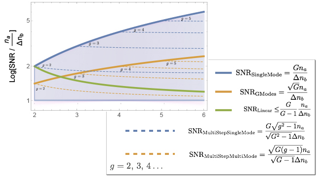
Figure 4.2: The signal-to-noise ratio results we have derived are plotted logarithmically. Here, the linear amplification scheme plotted is the phase insensitive one (Eq. 4.22). The dashed lines correspond to the multi-step amplification schemes in Eq. 4.26 and Eq. 4.27 and perform worse than their single-step counterparts. The fundamental limit is reached only by the single mode amplification scheme (Eq. 4.24) implementing ideal amplification. The trade-space is further filled in by considering additional noise modes that are not occupied by excitations deterministically.

Similarly, we consider multi-step amplification models

$$\textnormal{SNR}_{{\rm MultiStepSingleMode}} = \frac{G\sqrt{g^{2}-1}n_{a}}{\sqrt{G^{2}-1}\Delta n_{b}}$$ (4.26)

$$\textnormal{SNR}_{{\rm MultiStepMultiMode}} = \frac{\sqrt{G(g-1)}n_{a}}{\sqrt{G-1}\Delta n_{b}}.$$ (4.27)

These intermediate noise limits fill in the space between the optimal SNR in Eq. (4.24) and linear amplification as shown in Fig. 4.2. (Indeed, multi-step multi-mode amplification performs slightly worse than both linear mechanisms for $g=2$!)

In general, nonlinear amplification enables SNRs that, as functions of the total gain factor $G$, do not saturate with the gain $G$ and outperform what is possible with linear amplification. This is most apparent in the low temperature limit where the lack of zero-temperature noise for non-linear amplification (due to amplification taking place at a different frequency) is most prominent.

4.6 Single-photon pre-amplification

While this chapter focuses on the amplification part of the photodetection process, we now very briefly consider the pre-amplification process. We certainly cannot treat that part in full generality here and we adopt several simplifications in order to arrive at an important result concerning the suppression of thermal noise. First, we assume that we can decouple the amplification stage from the pre-amplification filtering [by having an irreversible step in between the two] such that filtering does not interfere negatively with the absorption/transduction part [26]. We then focus on just the time/frequency degree of one incoming photon. A single absorber with some resonance frequency $\omega_{0}$ able to absorb that single photon will act as a frequency filter. If the pre-amplification filtering is passive (easy to implement, but we certainly can go beyond this) and unitary (i.e., lossless: we consider this because we are interested in the fundamental limits of photodetection. Internal losses only degrade performance.), then frequency filtering is described by the linear transformation

$$\hat{a}_{{\rm out}}(\omega)=T(\omega)\hat{a}_{{\rm in}}(\omega)+R(\omega)\hat{c}_{{\rm in}}(\omega)$$ (4.28)

where $c_{{\rm in}}(\omega)$ is yet another internal bosonic detector mode at the same frequency as the input mode. Here $T(\omega)$ and $R(\omega)$ are “transmission” and “reflection” coefficients which satisfy $|T(\omega)|^{2}+|R(\omega)|^{2}=1$ and which are determined by the resonance structures internal to the photodetector. The amplification process that follows the initial absorption of the photon energy is applied to the operator $\hat{a}_{\rm out}(\omega)$ of Eq. (4.28), so that (explicitly displaying the different frequencies of the modes now) ideal amplification (single-mode and single-shot) is described by

$$\!\hat{b}^{\dagger}_{\rm out}(\omega^{\prime})\hat{b}_{\rm out}(\omega^{\prime})=\hat{b}^{\dagger}_{\rm in}(\omega^{\prime})\hat{b}_{\rm in}(\omega^{\prime})+G\hat{a}^{\dagger}_{\rm out}(\omega)\hat{a}_{\rm out}(\omega).$$ (4.29)

This makes rigorous the idea that one can amplify at any frequency, enabling the mantra that one should amplify at high (optical) frequencies [195]. Namely, thermal fluctuations at a frequency $\omega^{\prime}$ may be suppressed by choosing the reservoir mode frequency $\omega^{\prime}$ such that $\hbar\omega^{\prime}\gg kT$. This suppression is exponential: $\Delta n_{b}^{2}\propto\bar{n}_{b}\propto\exp(-\hbar\omega^{\prime}/kT)$. Note that number fluctuations in the internal mode $c_{{\rm in}}(\omega)$ at the input frequency will be amplified by the subsequent amplification process. However, one can in principle construct ideal detectors for light with a particular frequency $\omega_{0}$ [26], such that $|T(\omega_{0})|=1$ and hence $R(\omega_{0})=0$, avoiding internally generated dark counts at that particular frequency. If instead of a single monochromatic mode a small range of frequencies is amplified with differing probabilities (that is, a particular temporal mode), matching the amplification spectrum to the filtering spectrum is sufficient for reducing internally generated dark counts, as we will discuss in more detail in the next chapter.

4.7 Connections

The models for amplification considered here apply to other types of quantum measurement as well. For example, electron-shelving [31, 183, 184] is a well-known method to perform atomic state measurements. Here one particular atomic state (e.g., one of the hyperfine ground states of an ion) is coupled resonantly to a higher-lying excited state which can then decay back by fluorescence only to that same ground state. A laser tuned to that transition can then induce the atom to emit a macroscopic amount (visible by eye) of fluorescent light. In the language accompanying Eq. (4.2), the laser beam forms the first reservoir, while the second reservoir consists of vacuum modes that are filled with fluorescent light as described by Eq. (4.8). The gain factor $G$ (the number of fluorescence photons) is determined by the ratio of Einstein’s coefficients for spontaneous and stimulated emission and the total integration time. By placing the atom/ion inside a high-Q optical resonator (with resonant frequency $\omega^{\prime}$) we would reduce the number of output modes and thereby get closer to the optimum. The idea of placing a detector inside a resonant cavity is, of course, not new [196], but that idea is usually associated with increasing the coupling to light. Although we do have that effect as well, the main purpose here is to reduce the number of output modes, and thereby increase the SNR (Fig. 4.1).

A method similar to electron shelving (but using a collective metastable state of an atomic gas) was proposed in [197] for implementing high-efficiency photon counting with an, in principle, quantum nondemolition measurement. Our model describes that detector too and clarifies why such a measurement is possible; nonlinear amplification enables low-noise photon counting and does not destroy the input photons without an additional step as in Eq. (4.4).

In [177], a transformation similar to Eq. (4.2) is given: $n$ photons are directly converted to $Gn$ photons in a single mode. Though this transformation is unphysical (there is no way to preserve the commutator), a SNR is calculated that increases linearly with $G$ like our Eq. (4.24). However, the SNR found in [177] diverges for a photodetector with unit efficiency, which is not the case once fluctuations in the reservoir mode are properly taken into account as our results clarify.

In [175], Yang and Jacob propose an interesting model for amplification that makes use of a first-order phase transition for a collection of $N$ interacting spin-1/2 particles. These spins are coupled both to an input photon and to an output bosonic mode. The SNR (as we define it here) for that model scales as $\sqrt{N}$ while the gain $G$ of that model is linear in $N$. Thus, the SNR scales with $\sqrt{G}$ just as our Eq. (4.25): the number of spins in [175]’s model plays a similar role as our number of amplification modes.

4.8 Remarks

We discussed various linear and nonlinear amplification schemes for bosonic modes. For detecting few photons, we found that the latter add considerably less noise, leading to better signal-to-noise ratios, as exemplified in Eqs. (4.22)–(4.27). Unlike for linear amplification, number fluctuations in internal detector modes are not amplified, while the number of photons that we want to detect is amplified. All amplification schemes explicitly preserve the bosonic commutation relations.

While amplification into a single-mode may not be feasible in practice, it provides the fundamental lower limit to noise in photon-number measurements across amplification mechanisms. In practice, one may have many output modes and thus may find a SNR closer to Eq. (4.25), which is worse by a factor of $\sqrt{G}$ than the fundamental limit (but still better by a factor of $\sqrt{G}$ than linear amplification), or one may have multiple amplification steps as in Eq. (4.26), or both as in Eq. (4.27). To test this, we suggest that measurement of the gain dependence of the SNR for a given photodetector should provide a rough but useful indication of the underlying amplification mechanism.

Chapter 5 Measurement and Applications

The model of a SPD as an isolated two-level system is highly idealized. In a more realistic system, photodetection is an extended process wherein a photon is transmitted into the detector, interacting with the system and triggering a macroscopic change of the photodetector state (amplification) which can then be measured classically. Many theories of single-photon detection have been developed over the past century, [44, 47, 48, 49, 126, 50, 51, 127, 52, 26, 24, 25] and indeed there are numerous implementations of SPD technology [128, 129, 77, 22, 66, 23]. Across all systems, we have identified the three stages of transmission, amplification, and measurement as universal. In the previous two chapters, we have studied amplification and transmission in isolation, discussing the tradeoffs and limits that emerge for each stage individually. In this chapter, we will combine our results with a final quantum measurement and derive a POVM that incorporates all three stages quantum mechanically, extending our model to include fluctuations of system parameters. Then, in the remainder of this chapter we will discuss applications enabled by such a photo detecting system.

5.1 Realistic SPD POVMs

The time-dependent two-level system from the previous section enabling arbitrary wavepacket projection is incorporated into the three-stage model as the trigger for the amplification mechanism. This will enable us to still project onto arbitrary single-photon wavepackets, a result we will prove at the end of this section. We will assume in this analysis that the system is left on for a sufficient time such that the subnormalization of $\Psi(t)$ is minimal and ${\cal W}\approx 1$ (2.13).

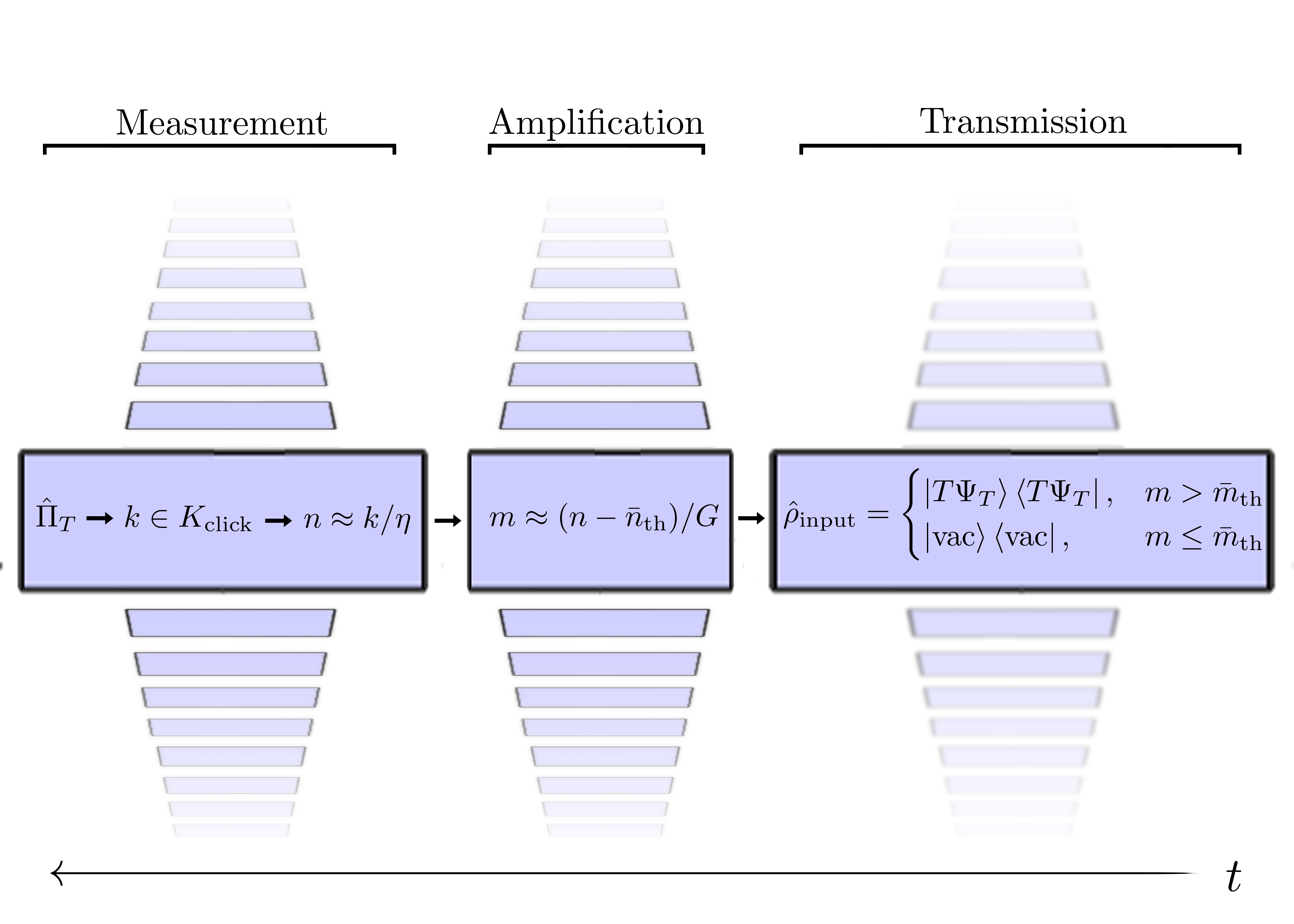
Figure 5.1: A POVM description of the three-stage model of photodetection, where the chain of inference (left to right) moves opposite the arrow of time, connecting a macroscopic “click” outcome to the state of the input field. A “click” outcome represented by the POVM element $\hat{\Pi}_{T}$ indicates ${k\in K_{\rm click}}$ excitations were measured in the final measurement with detection efficiency $\eta$. This retrodicts that ${n\approx k/\eta}$ (and, strictly, ${n\geq k}$) excitations were present post-amplification, either from thermal fluctuations or an amplification process. In turn, this indicates that ${m\approx(n-\bar{n}_{\rm th})/G\leq n}$ excitations were likely incident to the amplification process trigger, with $\bar{n}_{\rm th}$ the expected number of thermal excitations already in the amplification target mode. If $m$ is larger than the expected number of thermal excitations in the amplification trigger mode $\bar{m}_{\rm th}$, we conclude that one input photon of the form $\left|T\Psi_{T}\right\rangle\left\langle T\Psi_{T}\right|$ was likely present. In addition to the states written explicitly, there are other possible states where $k$, $n$, and $m$ deviate from their most likely values. These states (denoted by parallelograms) contribute to the POVM element, as the internal state of the photodetector is in general highly mixed. Nonetheless, in the end a SPD POVM element $\hat{\Pi}_{T}$ only projects onto the two input states $\left|T\Psi_{T}\right\rangle\left\langle T\Psi_{T}\right|$ and $\left|\rm vac\right\rangle\left\langle\rm vac\right|$, remaining relatively pure.

In the spirit of what a POVM does (connect present outcomes to probabilistic statements about quantum states in the past), we will begin our endeavor at the very end of the photodetection process following Fig. 5.1. Consider a macroscopic measurement performed at time $T$ with a binary response triggered by $k$ excitations measured in the amplified signal. Such a POVM can be written as a projector onto Fock states in the Hilbert space internal to the system

$$\hat{\Pi}_{T}=\sum\limits_{k\in K_{\rm click}}\left|k,\,T\right\rangle\left\langle k,\,T\right|.$$ (5.1)

Here, we have defined a set $K_{\rm click}$ that sets the threshold for how many amplification excitations must be measured to trigger a macroscopic detection event. At this stage, we can already see that the internal state the POVM projects onto is highly mixed, but this will not directly translate to an impure measurement on the Hilbert space of input photons. Indeed, this is what we would expect; we do not need to know precisely the internal state of the photodetector in order to use it to efficiently detect the presence of a single photon.

The macroscopic measurement performed on the amplified signal will, in general, be inefficient. We model this in a standard way [198], using a beamsplitter with frequency independent transmission amplitude $\sqrt{\eta}$. We can then rewrite the POVM element (5.1) so that it projects onto Fock states in the amplification target mode prior to the measurement

$$\hat{\Pi}_{T}=\sum\limits_{k\in K_{\rm click}}\sum\limits_{n=k}^{\infty}\Pr(n|k)\left|n,\,T\right\rangle\left\langle n\,T\right|$$ (5.2)

where we have defined

$$\Pr(n|k)={n\choose k}\eta^{k}(1-\eta)^{n-k}$$ (5.3)

the probability to detect $k$ excitations given that there were $n$ excitations in the output mode of the amplification process. An inefficiency $1-\eta$ affects photodetection by changing which post-amplification Fock states are projected onto: the larger $1-\eta$ is, the more post-amplification states $\left|n,\,T\right\rangle\left\langle n,\,T\right|$ will be projected onto intermediately by the same POVM element $\hat{\Pi}_{T}$, making it harder to distinguish between signal and noise.

We now move one step further back in the chain of inference (Fig. 5.1) so the POVM element $\hat{\Pi}_{T}$ projects onto the number of excitations $m$ input to the amplification trigger. Amplification is a generic feature of photodetection; without a macroscopic change in the internal state of a photodetector, there is no way to correlate detector outcomes with the presence of a single photon [199, 175, 200] (that is, without invoking additional single-excitation detectors in an argument circulus in probando). There are many interesting methods for implementing amplification [172, 197, 174, 52, 173, 199, 175, 200], but the fundamental quantum limit to amplification of any bosonic Fock state is achieved by a Schrödinger picture transformation [5]

$$\left|m\right\rangle_{\rm trig}\left|M\right\rangle_{\rm res}\left|N\right\rangle_{\rm targ}\longmapsto\left|m\right\rangle_{\rm trig}\left|M-Gm\right\rangle_{\rm res}\left|N+Gm\right\rangle_{\rm targ}$$

such that exactly $G$ excitations are transferred from the reservoir mode to the target mode for each excitation in the trigger mode. In using this expression we do impose a restriction that there must be $M>Gn$ excitations in the reservoir mode, but restrictions of this type are to be expected (the energy for amplification must come from somewhere) and we will be most interested in few photons ($n=0,1,2$) in this analysis. In most physical platforms $G$ will fluctuate, as will other (classical) system parameters which we will return to at the end of this section. (Exceptions do exist; for Hamiltonians that implement deterministic amplification schemes [with small integer values for $G$] see Ref. [182].) However, even with a definite gain factor $G$ and number of input excitations $m$, we will still not end up with exactly $n=N+Gm$ excitations if the target mode is initially in a thermal state with mean occupation number $\bar{N}$ (as opposed to a Fock state with exactly $N$ excitations). We now assume this, writing the state of the target mode in the Fock basis

$$\hat{\rho}_{\rm targ}^{(th)}=\sum\limits_{N=0}^{\infty}P^{\rm th}_{N,\,T}|N,\,T\rangle\!\langle N,\,T|,$$ (5.5)

with the probability for $N$ thermal excitations given by

$$P^{\rm th}_{N}=\frac{1}{1+\bar{N}}\left(\frac{\bar{N}}{1+\bar{N}}\right)^{N};\,\bar{N}=\frac{1}{e^{\frac{\hbar\omega^{\prime}}{k_{b}T}}-1},$$ (5.6)

where $\omega^{\prime}$ and $k_{B}T$ are the frequency and the thermal energy of the target mode. Assuming the ideal amplification scheme in (5.1), we now write the POVM element $\hat{\Pi}_{k}$ in terms of the number $m$ excitations that trigger the application mechanism

$$\!\hat{\Pi}_{T}=\sum\limits_{k\in K_{\rm click}}\sum\limits_{n=k}^{\infty}\Pr(n|k)\sum\limits_{m=0}^{{\rm Int}_{-}[\frac{n}{G}]}P^{\rm th}_{n-Gm}\left|\Psi_{T}\right\rangle\left\langle\Psi_{T}\right|^{\otimes m}$$

where we define $\left|\Psi_{T}\right\rangle\left\langle\Psi_{T}\right|^{\otimes 0}=|{\rm vac}\rangle\langle{\rm vac}|$, $P^{\rm th}_{N}=0$ for $N<0$, and the function ${\rm Int}_{-}$ rounding down to the nearest integer. We can now see the benefit of having a large gain factor G; it shifts the probability distribution over $n$ that corresponds to non-zero excitations in the trigger mode, minimizing its overlap with the probability distribution for zero excitations. In this way, one can dramatically reduce the background noise (dark counts) without decreasing signal by changing the minimum value of the set $K_{\rm click}$. In (5.1) we have reintroduced the state $\left|\Psi_{T}\right\rangle$ defined in (2.2) as the state projected onto by the trigger mechanism. As in the previous section, we will assume a time-dependent resonance frequency $\Delta(t)$ and decay rate $\kappa(t)$ so that arbitrary pulse-shaping is possible.

The POVM element in (5.1) now projects onto quantum states internal to the photodetector. We need to connect the internal continuum of states coupled to the amplification trigger to the external continuum containing the photons we wish to detect (the transmission stage in Fig. 5.1). This is accomplished by introducing a two-sided quantum network to serve as the transmission stage [108]. Any such network is completely described by a single complex frequency-dependent transmission coefficient $T(\omega)$ (related to a reflection coefficient at each frequency via $|T(\omega)|^{2}+|R(\omega)|^{2}=1$ and $R(\omega)T^{*}(\omega)+R^{*}\omega)T(\omega)=0$). We now invoke the single-photon assumption so that there is at most a single excitation input to the quantum network. Any other excitations present in the internal continuum will be from internally-generated thermal fluctuations reflected by the quantum network back to the trigger mechanism. In this way, we can construct a POVM element that projects onto product-states $\left|\psi_{\rm ex}\right\rangle\left\langle\psi_{\rm ex}\right|\otimes\left|\psi_{\rm in}\right\rangle\left\langle\psi_{\rm in}\right|$ of the external and internal continua

$$\!\!\!\!\!\!\!\!\!\!\!\!\!\!\!\!\!\!\!\!\!\!\!\!\hat{\Pi}_{T} = \sum\limits_{k\in K_{\rm click}}\sum\limits_{n=k}^{\infty}\Pr(n|k)\left(P^{\rm th}_{n}|{\rm vac}\rangle\langle{\rm vac}|\otimes|{\rm vac}\rangle\langle{\rm vac}|\phantom{\sum\limits_{m=1}^{{\rm Int}_{-}[\frac{n}{G}]}}\right.$$ (5.8)

$$+ \sum\limits_{m=1}^{{\rm Int}_{-}[\frac{n}{G}]}P^{\rm th}_{n-Gm}\rho^{2m}|{\rm vac}\rangle\langle{\rm vac}|\otimes\left|R\Psi_{T}\right\rangle\left\langle R\Psi_{T}\right|^{\otimes m}\phantom{\sum\limits_{m=1}^{{\rm Int}_{-}[\frac{n}{G}]}}$$

$$+ \left.\sum\limits_{m=1}^{{\rm Int}_{-}[\frac{n}{G}]}mP^{\rm th}_{n-Gm}\tau^{2}\rho^{2(m-1)}\left|T\Psi_{T}\right\rangle\left\langle T\Psi_{T}\right|\otimes\left|R\Psi_{T}\right\rangle\left\langle R\Psi_{T}\right|^{\otimes m-1}\right).$$

The first line corresponds to dark counts generated from thermal excitations post-amplification and the second line corresponds to dark counts generated by thermal excitations that then trigger the amplification mechanism. Only the third line contains a projection onto a photon to be detected. (The multiplicative factor $m$ in the third line is combinatorial in origin: $m$ total excitations in the trigger mode with $m-1$ generated from thermal fluctuations.) In writing (5.8) we have defined transmitted and reflected normalized single-photon states and coefficients

$$\left|T\Psi_{T}\right\rangle = \frac{1}{\tau}\int_{-\infty}^{\infty}\,d\omega\tilde{\Psi}(\omega)T^{*}(\omega)e^{i\,\omega\,T}\hat{a}^{\dagger}(\omega)\left|\textnormal{vac}\right\rangle$$

$$\left|R\Psi_{T}\right\rangle = \frac{1}{\rho}\int_{-\infty}^{\infty}\,d\omega\tilde{\Psi}(\omega)R^{*}(\omega)e^{i\,\omega\,T}\hat{b}^{\dagger}(\omega)\left|\textnormal{vac}\right\rangle$$

$$\tau = \sqrt{\int d\omega|\tilde{\Psi}(\omega)|^{2}|T(\omega)|^{2}}$$

$$\rho = \sqrt{\int d\omega|\tilde{\Psi}(\omega)|^{2}|R(\omega)|^{2}}$$ (5.9)

where $\hat{a}^{\dagger}$ and $\hat{b}^{\dagger}$ are the creation operators for the external and internal continua and we have defined a Fourier-transformed wavepacket for the amplification trigger mode $\tilde{\Psi}(\omega)={\rm FT}[\sqrt{\kappa(t)}\Psi(t)]$. We can now see how pre-amplification dark counts (the second line of (5.8)) can be suppressed: by reducing the overlap of $|\tilde{\Psi}(\omega)|^{2}$ and $|R(\omega)|^{2}$, that is, by only amplifying the frequencies we wish to detect so that $\rho^{2}\ll 1$. In this case, the POVM element (5.8) will be dominated by the $m=1$ term of the third line (the signal to be detected with no thermal excitations), as well as potentially the first line. (To reiterate, these are dark counts post-amplification, but these can be reduced by amplifying at a high frequency such that $\hbar\omega^{\prime}\gg k_{B}T$, where $\omega^{\prime}$ and $k_{B}T$ are the frequency and thermal energy of the target mode.)

Finally, we trace over the internal continuum, which we assume is in a thermal state with thermal energy $k_{B}T^{\prime}$ so the POVM projects onto the external continua only

$$\hat{\Pi}_{T} = \sum\limits_{k\in K_{\rm click}}\sum\limits_{n=k}^{\infty}\Pr(n|k)\left(\sum\limits_{m=0}^{{\rm Int}_{-}[\frac{n}{G}]}P^{\rm th}_{n-Gm}P^{{}^{\prime}\rm th}_{m}\rho^{2m}\right.|{\rm vac}\rangle\langle{\rm vac}|$$ (5.10)

$$+ \left.\sum\limits_{m=1}^{{\rm Int}_{-}[\frac{n}{G}]}mP^{\rm th}_{n-Gm}P^{{}^{\prime}\rm th}_{m-1}\tau^{2}\rho^{2(m-1)}\left|T\Psi_{T}\right\rangle\left\langle T\Psi_{T}\right|\right)$$

$$\equiv w_{0}|{\rm vac}\rangle\langle{\rm vac}|+w_{T}\left|T\Psi_{T}\right\rangle\left\langle T\Psi_{T}\right|$$

where in the last line we have absorbed the sums in front of the two projectors into weights so that the POVM element has the form of (1.9) and with $P^{{}^{\prime}\rm th}_{j}$ the probability to have $j$ excitations (now in the non-monochromatic reflected mode defined in (5.1)). For a finite detector on-time $T_{0}>-\infty$, the weights $w_{0}$ and $w_{T}$ will be slightly less than in (5.10) due to wavepacket sub-normalization (2.13). However, this deviation is negligible provided the detector is left on for a time comparable to the temporal mode’s width.

We now reconsider the question of projecting onto an arbitrary wavepacket, including the full quantum description. We find that this is possible to do in principle, provisio $T(\omega)$ is nowhere zero (except at infinity), a result we will now prove. That is, we can ensure that the single-photon wavepacket $\left|T\Psi_{T}\right\rangle$ has any desired (smooth) shape and will be projected onto with a high-efficiency and high-purity measurement.

Proof.— Consider a photon with complex normalized spectral wavepacket $\tilde{f}(\omega)$. If detection is achieved with a time-dependent two-level system preceded by a quantum network with filtering transmission function $T(\omega)$, the system will project onto a state $\left|T\Psi_{T}\right\rangle$ as defined in (5.1). In the low-noise limit this will be the only state projected onto by the (pure) POVM element. From the Born rule, the probability of detection will be

$$P_{T}=w_{T}\frac{1}{\tau^{2}}\left|\int_{-\infty}^{\infty}d\omega\tilde{f}(\omega)\tilde{\Psi}(\omega)T^{*}(\omega)\right|^{2}$$ (5.11)

with $w_{T}$ the overall weight given by (5.10) and maximum possible detection efficiency, which can be arbitrarily close to unity. It is possible to achieve $P_{T}=w_{T}$ (mode-matched detection) in (5.11) if and only if

$$\tilde{\Psi}(\omega)=\frac{\tilde{f}^{*}(\omega)}{T(\omega)}e^{i\omega T}.$$ (5.12)

From (2.12), we know that it is possible to generate an arbitrary temporal wavepacket ${\rm FT}^{-1}[\tilde{\Psi}(\omega)]=\sqrt{\kappa(t)}\Psi(t)$ from a time-dependent two-level system. The Fourier transform of a continuous smooth function is itself smooth and continuous. Thus, if the right hand side of (5.12) is a well-defined spectral wavepacket (smooth and continuous), one can find functions $\kappa(t)$ and $\Delta(t)$ such that $\tilde{\Psi}(\omega)$ has the form of (5.12). ∎

Remark.— Arbitrary wavepacket detection (and thus Fourier-limited simultaneous measurements of time and frequency) is in principle possible only when there are no photonic band gaps induced by the filter; if $T(\omega^{\prime})=0$ for some frequency $\omega^{\prime}$, there is simply no way to compensate for the lost information about $\omega^{\prime}$. Photonic band gaps are a generic feature of parallel (and hybrid) quantum networks [108] as well as certain non-Markovian systems [201]. Network/reservoir engineering must be employed to ensure any $\omega^{\prime}$ where $T(\omega^{\prime})=0$ is not a frequency of interest.

The POVM $\{\hat{\Pi}_{T},\,\hat{\Pi}_{0}\}$ with $\hat{\Pi}_{T}$ defined in (5.10) and $\hat{\Pi}_{0}=\hat{\mathds{1}}-\hat{\Pi}_{T}$ provides a complete description of the single-photon detection process that is fully quantum from beginning to end (Fig. 5.1). However, there is a final element that must be considered to make the description applicable to labratory systems: classical parameter fluctuations. For continuous parameter fluctuations over any system parameter or set of system parameters $X$, these are naturally incorporated

Symbol	System Parameter	Fluctuations
$K_{\rm click}$	Macroscopic Detection Threshold	$w_{0},\,w_{T}$
$\eta$	Macroscopic Detection Efficiency	$w_{0},\,w_{T}$
$k_{B}T$	Target Mode Thermal Energy	$w_{0},\,w_{T}$
$\omega^{\prime}$	Target Mode Frequency	$w_{0},\,w_{T}$
$G$	Amplification Gain	$w_{0},\,w_{T}$
$\tilde{\Psi}(\omega)$	Amplification Trigger Mode	$w_{0},\,w_{T},\,\left|T\Psi_{T}\right\rangle$
$k_{B}T^{\prime}$	Internal Continuum Thermal Energy	$w_{0},\,w_{T}$
$T(\omega)$	Transmission Coefficient	$w_{0},\,w_{T}\,\left|T\Psi_{T}\right\rangle$

Table 5.1: The effects of classical fluctuations in system parameters on the final POVM: either the weights and states are changed, or only the weights are changed. The fluctuations over the functions $\tilde{\Psi}(\omega)$ and $T(\omega)$ (and thus $R(\omega)$ by unitarity) could be caused by fluctuations in other system parameters (decay rates, resonances) internal to those functions. A subset of fluctuations in $\tilde{\Psi}(\omega)$ are fluctuations in the time of detection $T$. Importantly, these shift the wavepacket $\Psi(t)$ projected onto, resulting in a mixed measurement with larger temporal uncertainty (jitter) that depends on the ratio of the fluctuations in $T$ to the width of the temporal wavepacket.

(5.13)

$$\!\hat{\Pi}_{T}=\int dX{\rm Pr}(X)\left(w_{0}|{\rm vac}\rangle\langle{\rm vac}|+w_{T}\left|T\Psi_{T}\right\rangle\left\langle T\Psi_{T}\right|\right)$$

where we have assumed a (known) probability distribution ${\rm Pr}(X)$. In (5.13), the system parameter(s) $X$ could be such that only the weights $w_{0}$ and $w_{T}$ depend on $X$, or $X$ could be such that the state $\left|T\Psi_{T}\right\rangle$ depends on $X$ as well (for a summary, see Tbl. 5.1). In the case of the latter, the POVM will become less pure and will need rediagonalization to determine which states are projected onto. This final POVM not only includes ignorance about the internal state of the photodetector as was depicted in Fig. 5.1, but also classical ignorance about the state of the photodetector due to system-lab interactions.

5.2 Applications

Using the time-dependent two-level system, we are able to project onto orthogonal quantum states (Fig. 5.2). This enables efficient detection of photonic qubits, an essential component of any quantum internet [203, 204]. More generally, temporal modes provide a complete framework for quantum information science [205], with efficient detection of orthogonal modes (and their superpositions to create mutually unbiased bases) a key ingredient. Fully manipulable temporal modes also play a key role in error-corrected quantum transduction [206], where a time-reversed temporal mode can restore an unknown superposition in a qubit. Here, efficient detection of arbitrary temporal modes is essential so that quantum jumps out of the dark state are efficiently heralded.

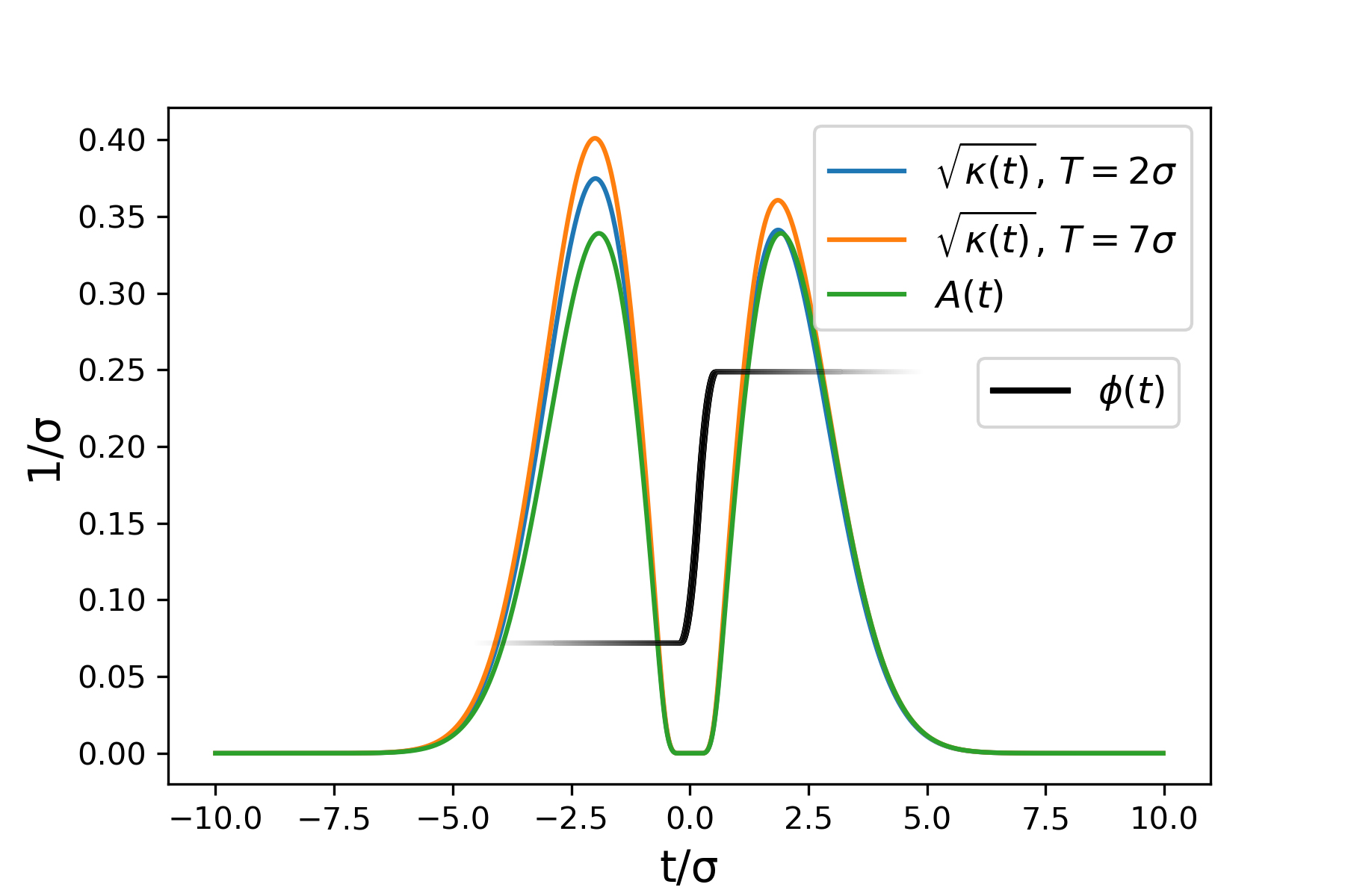
Figure 5.2: The time-dependent coupling $\kappa(t)$ that generates a wavepacket exactly orthogonal to the minimum uncertainty Gaussian wavepacket in Fig. 2.3 are plotted for times of detection ${T=2\sigma}$ (${{\cal W}=0.72}$) and ${T=7\sigma}$ (${{\cal W}=1-10^{-5}}$) and detector on-time ${T_{0}=-\infty}$. The wavepacket’s time-dependent amplitude $A(t)$ (depicted in the rotating frame) is an approximate first-order Hermite-Gaussian pulse, where the singular region of zero as been expanded with half-width of ${z=0.5\sigma}$. In this way, the wavepacket’s phase (solid black line, not to scale) can go from $0$ to $\pi$ in a finite time, whereas the Heaviside phase-flip in the exact Hermite-Gaussian pulse requires an unphysical delta-function detuning (second line of (2.2). Both the phase and amplitude have been convolved with a triangular smoothing function with full-width ${s=0.5\sigma}$, ensuring $A(t)$ is continuously differentiable to first order [207, 208], which is pre-requisite for solving the Bernoulli equation (2.21). For any finite ${z\geq s>0}$ the phase flip [here implemented with a triangular detuning $\Delta(t)$] occurs while the amplitude is zero. This ensures exact orthogonality of the approximate first-order Hermite-Gaussian to the gaussian pulse. In the limit ${s,z\rightarrow 0}$, an exact first-order Hermite-Gaussian is recovered. This smoothing procedure generalizes to higher order Hermite-Gaussian pulses, forming a mutually unbiased basis for efficient detection of higher dimensional qudits [205].

High-purity measurements that project onto orthogonal single-photon wavepackets also enable super-resolved measurements [209]. Suppose we have two single-photon sources emitting almost identical pure states differing slightly in either emission time or central frequency

$$\left|\tilde{\phi}_{1}\right\rangle =\frac{\left|\phi_{1}\right\rangle+\sqrt{\epsilon}\left|\phi_{2}\right\rangle}{\sqrt{1+\epsilon}}$$

$$\left|\tilde{\phi}_{2}\right\rangle =\frac{\left|\phi_{1}\right\rangle-\sqrt{\epsilon}\left|\phi_{2}\right\rangle}{\sqrt{1+\epsilon}}$$ (5.14)

with $\left\langle\tilde{\phi}_{1}|\tilde{\phi}_{2}\right\rangle$ real, $\epsilon\ll 1$, and $\left\langle\phi_{1}|\phi_{2}\right\rangle=0$. Alternatively, we may imagine a single source of light but the light we receive may have either been slightly Doppler-shifted or it may have been slightly delayed.

Suppose now that we receive one photon that could equally likely be from either source so that our input state is

$$\hat{\rho}=\frac{1}{2}\left|\tilde{\phi}_{1}\right\rangle\left\langle\tilde{\phi}_{1}\right|+\frac{1}{2}\left|\tilde{\phi}_{2}\right\rangle\left\langle\tilde{\phi}_{2}\right|.$$ (5.15)

If we can measure both $\hat{\Pi}_{1}=\eta\left|\phi_{1}\right\rangle\left\langle\phi_{1}\right|$ and $\hat{\Pi}_{2}=\eta\left|\phi_{2}\right\rangle\left\langle\phi_{2}\right|$ (that is, if we have separate photodetectors with these (pure) POVM elements, or a single non-binary-outcome photodetector), then we find the probability of clicks

$$P_{1} = {\rm Tr}\left[\hat{\Pi}_{1}\hat{\rho}\right]=\eta\frac{1}{1+\epsilon}$$

$$P_{2} = {\rm Tr}\left[\hat{\Pi}_{2}\hat{\rho}\right]=\eta\frac{\epsilon}{1+\epsilon}$$ (5.16)

so that the ratio of clicks gives a direct estimate of $\epsilon$, even for low efficiency $\eta$. Here all that is needed for time-frequency domain super-resolved measurement of $\epsilon$ are SPDs with time-dependent couplings and resonance frequencies as opposed to nonlinear optics [210].

In traditional quantum key distribution (QKD) schemes (that is, not measurement device independent (MDI)-QKD), specification of the measurement POVM is essential to robust security proofs [211, 212, 213]. Here, we have verified several assumptions about an eves-dropper’s capabilities common in security proofs: that high-purity measurements are possible, that high efficiency measurements are possible, and (for continuous-variable (CV)-QKD proofs) minimum time-frequency uncertainty measurements are possible. In particular for CV-QKD, an eavesdropper can perform measurements that project onto variable-width spectral modes, disrupting temporal correlations between Alice and Bob (who are assumed to use fixed time-frequency bins) [214]. Here, the capacity to adjust the width of the spectral mode $\tilde{\Psi}(\omega)$ provides Alice and Bob a new strategy to mitigate Eve’s attack and extract a secure key.

More generally, detector tomography [215, 95, 94, undeen2009, 94, 216] is an important tool across implementations of single-photon and number-resolved photodetection. Real-time tomography could be useful in QKD protocols resistant to “trojan-horse attacks” [217] or any SPD platform subject to time-dependent environmental parameter fluctuations: for instance, atmospheric turbulence in MDI-QKD [218] or interplanetary medium in deep space classical communications [219]. Recently tomography speed-ups have been achieved using machine learning assisted tomography protocols [220]. The POVMs derived in this thesis provide priors which can further speed up detector tomography [221]. These include approximate effects of environmental fluctuations as outlined in Fig. 3.1 and a global optimum POVM for single-photon detection (5.10) which can be used to incorporate detector calibration and optimization into in situ tomographic protocols.

Chapter 6 Conclusions

Having constructed a fully quantum model incorporating the three stages of photodetection (transmission, amplification, and measurement), we can now discuss the fundamental limits and tradeoffs inherent to photodetection as a whole.

We have constructed single-photon measurements that are fundamentally limited in two ways simultaneously: the first is that they can project onto Fourier-limited (Gaussian) time-frequency states as illustrated in Fig. 2.3, and the second is that the amplification scheme reaches a Heisenberg-limited (linear in the gain $G$) signal-to-noise ratio, surpassing the standard quantum limit (a signal-to-noise ratio going like of $\sqrt{G}$). Achieving these simultaneously is possible in principle with no drawback. Indeed, the only stringent tradeoff we encounter in this analysis is between efficiency and photon counting rate, which becomes substantial when an SPD is reset at a faster rate than $\sim 1/\Delta t$. (The photon does not have sufficient time to excite the two-level system with high probability before the system is reset.) For other figures of merit, we find that they are either independent, or deteriorate together. While it does appear from (5.10) that improving efficiency also increases dark counts, these are decoupled by ensuring the coefficient $\rho\ll 1$—that is, by making $T(\omega)$ broader than $\tilde{\Psi}(\omega)$. While it is commonsense that one should only amplify the frequencies they wish to detect, our work clarifies how enormously important this is. The dark counts produced in this way are insuperable; they cannot be removed post-amplification without removing the single-photon signal as well.

One optimistic conclusion from our work is that, while there are emergent tradeoffs to consider when constructing SPDs due to their multi-stage nature, these are generally avoidable with foresight and engineering. For instance, using a parallel network allows one to simultaneously optimize transmission efficiency $|T(\omega)|^{2}$, spectral bandwidth (3.1), and frequency dependent group delay (3.3) despite the individual tradeoffs present for other network types. Using a time-dependent amplification trigger, it is possible to still achieve Fourier-limited simultaneous measurements of time and frequency provided no frequencies of interest have been removed from the signal (that is, destructive interference has not resulted in $T(\omega)=0$) as demonstrated in (5.12). While some noise is unavoidable, minimal post-amplification arbitrarily high signal can be reached by amplifying into fewer modes even at room temperature by amplifying at higher frequencies. Furthermore, detection of a particular arbitrary wavepacket changes pre-amplification dark counts; the functions $T(\omega)$ and $\tilde{\Psi}(\omega)$ both determine the projected wavepacket $\tilde{f}(\omega)=T(\omega)\tilde{\Psi}(\omega)e^{-i\omega T}$ and are interchangeable up to complex conjugation. However, they have different roles in determining dark counts. One can significantly reduce pre-amplification dark counts by ensuring that the transmission stage $T(\omega)$ has a broader spectrum than the trigger mechanism $\tilde{\Psi}(\omega)$; pre-amplification dark counts go to zero as the reflection function $R(\omega)$ and trigger mechanism spectrum $\tilde{\Psi}(\omega)$ become orthogonal.

Another conclusion from this work is also rather optimistic. Here we have given a quantum description of an entire single-photon detection process projecting onto arbitrary single-photon states and the only fundamental limitations encountered are Heisenberg and Fourier limits. Incorporating realistic descriptions of amplification and a final measurement reduce efficiency and increase dark counts, but even so a Heisenberg-limited measurement is still achievable in principle. Similarly, incorporating the filtering of a first irreversible step does not impede implementation of Fourier-limited measurements provided no frequencies are completely blocked from entering the trigger mechanism. Even considering parameter fluctuations (5.13) in the two internal thermal energies $k_{B}T$ and $k_{B}T^{\prime}$, amplification frequency $\omega^{\prime}$, and amplification gain factor $G$—which are unavoidable in any realistic system—Fourier limited time-frequency measurements are achieved. To our knowledge, this works contains the first proposed quantum procedure for reaching Fourier-limited time-frequency measurements in a realistic quantum system. This is a fundamental limit to SPD performance enforced by foundational quantum theory, and provides a limit to any precision measurements involving time and frequency. Furthermore, probing Heisenberg limits paves the way for future experimental tests of quantum theory.

References

- Hamilton and Cairns [1961] Edith Hamilton and Huntington Cairns, editors. The Collected Dialogues of Plato. Princeton University Press, 1961.
- Croskerry et al. [2017] Pat Croskerry, Karen S. Cosby, Mark L. Graber, and Hardeep Singh. Diagnosis: Interpreting the Shadows. CRC Press, 2017.
- Nurdin et al. [2016] Hendra Ishwara Nurdin, Matthew R. James, and Naoki Yamamoto. Perfectly capturing traveling single photons of arbitrary temporal wavepackets with a single tunable device. arXiv preprint arXiv:1609.05643, 2016.
- Gardiner and Collett [1985] C. W. Gardiner and M. J. Collett. Input and output in damped quantum systems: Quantum stochastic differential equations and the master equation. Phys. Rev. A, 31(6):3761, 1985.
- Propp and van Enk [2019a] Tzula B. Propp and Steven J. van Enk. On nonlinear amplification: improved quantum limits for photon counting. Opt. Express, 27(16):23454, 2019a.
- Burton [1945] Harry Edwin Burton. The optics of Euclid. J. Opt. Soc. Am., 35(5):357–372, 1945.
- Hogendijk [2003] J. P. Hogendijk. The enterprise of science in Islam : new perspectives. MIT Press, Cambridge, Mass, 2003.
- Jacobs [2012] Fredrika H. Jacobs. Review of “Renaissance Theories of Vision” by John Shannon Hendrix and Charles H. Carman. caa.reviews, 2012.
- Khan [2007] Sameen Ahmed Khan. Arab origins of the discovery of the refraction of light. Optics and Photonics News, 18:22–23, 10 2007.
- King [1955] Henry C King. The history of the telescope. Sky Publishing Corp., Cambridge, Mass., 1955.
- Zubairy [2016] M. Suhail Zubairy. A very brief history of light. In Optics in Our Time, pages 3–24. Springer International Publishing, 2016.
- Bosanac [1998] S.D. Bosanac. Semiclassical theory of compton and photoelectric effects. The European Physical Journal D, 1(3):317–327, 1998.
- Compton [1923] Arthur H. Compton. A quantum theory of the scattering of x-rays by light elements. Physical Review, 21(5):483–502, 1923.
- Einstein [1916a] Albert Einstein. Strahlungs-Emission und Absorption nach der Quantentheorie. Deutsche Physikalische Gesellschaft, 18:318–323, 1916a.
- Peskin and Schroeder [1995] Michael E. Peskin and Daniel V. Schroeder. An Introduction to quantum field theory. Addison-Wesley, Reading, USA, 1995.
- Yuen and Shapiro [1978] Horace P. Yuen and Jeffrey H. Shapiro. Quantum statistics of homodyne and heterodyne detection. In Coherence and Quantum Optics IV, pages 719–727. Springer US, 1978.
- Collett et al. [1987] M. J. Collett, R. Loudon, and C.W. Gardiner. Quantum theory of optical homodyne and heterodyne detection. Journal of Modern Optics, 34(6-7):881–902, 1987.
- Merriam-Webster [2009] Merriam-Webster. Merriam-Webster Online Dictionary, 2009.
- Hadfield [2009] Robert H. Hadfield. Single-photon detectors for optical quantum information applications. Nature Photonics, 3(12):696–705, 2009. ISSN 1749-4885, 1749-4893.
- Rosfjord et al. [2006] Kristine M. Rosfjord, Joel K. W. Yang, Eric A. Dauler, Andrew J. Kerman, Vikas Anant, Boris M. Voronov, Gregory N. Goltsman, and Karl K. Berggren. Nanowire single-photon detector with an integrated optical cavity and anti-reflection coating. Opt. Express, 14(2):527, 2006.
- Sunter and Berggren [2018] Kristen A. Sunter and Karl K. Berggren. Optical modeling of superconducting nanowire single photon detectors using the transfer matrix method. Appl. Opt, 57(17):4872, 2018. ISSN 1559-128X, 2155-3165.
- Marsili et al. [2013] F Marsili, Varun B Verma, Jeffrey A Stern, S Harrington, Adriana E Lita, Thomas Gerrits, Igor Vayshenker, Burm Baek, Matthew D Shaw, and Richard P Mirin. Detecting single infrared photons with 93 percent system efficiency. Nat. Photonics, 7(3):210, 2013.
- Wollman et al. [2017] Emma E. Wollman, Varun B. Verma, Andrew D. Beyer, Ryan M. Briggs, B. Korzh, Jason P. Allmaras, F. Marsili, Adriana E. Lita, R. P. Mirin, and S. W. Nam. Uv superconducting nanowire single-photon detectors with high efficiency, low noise, and 4 k operating temperature. Optics Express, 25(22):26792–26801, 2017.
- Matekole et al. [2018] Elisha S Matekole, Hwang Lee, and Jonathan P Dowling. Limits to atom-vapor-based room-temperature photon-number-resolving detection. Phys. Rev. A, 98(3):033829, 2018.
- Léonard et al. [2019] François Léonard, Michael E. Foster, and Catalin D. Spataru. Prospects for Bioinspired Single-Photon Detection Using Nanotube-Chromophore Hybrids. Scientific Reports, 9(1):3268, 2019. ISSN 2045-2322.
- Young et al. [2018a] Steve M Young, Mohan Sarovar, and François Léonard. Fundamental limits to single-photon detection determined by quantum coherence and backaction. Phys. Rev. A, 97(3):033836, 2018a.
- Zhang et al. [2018] Yang Zhang, Yang Wu, Xiaoxin Wang, Lei Ying, Rahul Kumar, Zongfu Yu, Eric R. Fossum, Jifeng Liu, Gregory Salamo, and Shui-Qing Yu. Detecting single photons using capacitive coupling of single quantum dots. ACS Photonics, 5(5):2008–2021, 2018.
- Jahani et al. [2020] Saman Jahani, Li-Ping Yang, Adrián Buganza Tepole, Joseph C. Bardin, Hong X. Tang, and Zubin Jacob. Probabilistic vortex crossing criterion for superconducting nanowire single-photon detectors. Journal of Applied Physics, 127(14):143101, 2020.
- Planck and Masius [1914] M. Planck and M. Masius. The Theory of Heat Radiation. Blakiston, 1914.
- Einstein [1916b] Albert Einstein. Zur Quantentheorie der Strahlung. Mitteilungen der Physikalischen Gessellschaft Zürich, 18:47–62, 1916b.
- Dehmelt [1982] Hans G. Dehmelt. Monoion oscillator as potential ultimate laser frequency standard. IEEE transactions on instrumentation and measurement, (2):83–87, 1982.
- Dirac [1927] Paul Adrien Maurice Dirac. The quantum theory of the emission and absorption of radiation. Proceedings of the Royal Society of London. Series A, Containing Papers of a Mathematical and Physical Character, 114(767):243–265, 1927.
- Wigner [1927] E. Wigner. Einige folgerungen aus der schrödingerschen theorie für die termstrukturen. Zeitschrift für Physik, 43(9-10):624–652, September 1927.
- Oppenheimer [1930] J. R. Oppenheimer. Note on the theory of the interaction of field and matter. Physical Review, 35(5):461–477, 1930.
- Fermi [1932] Enrico Fermi. Quantum theory of radiation. Rev. Mod. Phys., 4:87–132, 1932.
- Bloch and Nordsieck [1937] F. Bloch and A. Nordsieck. Note on the radiation field of the electron. Physical Review, 52(2):54–59, 1937.
- Weisskopf [1939] V. F. Weisskopf. On the self-energy and the electromagnetic field of the electron. Physical Review, 56(1):72–85, 1939.
- Tomonaga [1946] S. Tomonaga. On a relativistically invariant formulation of the quantum theory of wave fields. Progress of Theoretical Physics, 1(2):27–42, 1946.
- Schwinger [1948] Julian Schwinger. Quantum electrodynamics. i. a covariant formulation. Physical Review, 74(10):1439–1461, 1948.
- Feynman [1949] R. P. Feynman. Space-time approach to quantum electrodynamics. Physical Review, 76(6):769–789, 1949.
- Weisskopf and Wigner [1930] V. Weisskopf and E. Wigner. Berechnung der natürlichen linienbreite auf grund der diracschen lichttheorie. Zeitschrift für Physik, 63(1-2):54–73, January 1930. 10.1007/bf01336768. URL https://doi.org/10.1007/bf01336768.
- Brown and Twiss [1956] R. Hanbury Brown and R. Q. Twiss. A test of a new type of stellar interferometer on sirius. Nature, 178(4541):1046–1048, 1956.
- Purcell [1956] E. M. Purcell. The question of correlation between photons in coherent light rays. Nature, 178(4548):1449–1450, 1956.
- Glauber [1963] Roy J. Glauber. The quantum theory of optical coherence. Phys. Rev., 130:2529–2539, 1963.
- Steck [revision 0.12.3, 25 October 2018] Daniel A. Steck. Quantum and Atom Optics,. Available online at http://steck.us/teaching, revision 0.12.3, 25 October 2018.
- Mandel [1959] L. Mandel. Fluctuations of photon beams: The distribution of the photo-electrons. Proceedings of the Physical Society, 74(3):233–243, 1959.
- Kelley and Kleiner [1964] P. L. Kelley and W. H. Kleiner. Theory of electromagnetic field measurement and photoelectron counting. Phys. Rev., 136:A316–A334, 1964.
- Scully and Lamb [1969] Marlan O. Scully and Willis E. Lamb. Quantum theory of an optical maser. III. Theory of photoelectron counting statistics. Phys. Rev., 179(2):368, 1969.
- Yurke and Denker [1984] Bernard Yurke and John S. Denker. Quantum network theory. Phys. Rev. A, 29(3):1419, 1984.
- Ueda [1999] M. Ueda. Probability-density-functional description of quantum photodetection processes. Quantum Opt.: J. Eur. Opt. Soc. B, 1:131, 01 1999.
- Schuster et al. [2005] D. I. Schuster, Andreas Wallraff, Alexandre Blais, L. Frunzio, R.-S. Huang, J. Majer, S. M. Girvin, Schoelkopf, and RJ. ac Stark shift and dephasing of a superconducting qubit strongly coupled to a cavity field. Phys. Rev. Lett., 94(12):123602, 2005.
- Clerk et al. [2010] Aashish A Clerk, Michel H Devoret, Steven M Girvin, Florian Marquardt, and Robert J Schoelkopf. Introduction to quantum noise, measurement, and amplification. Rev. Mod. Phys., 82(2):1155, 2010.
- Jaynes and Cummings [1963] E.T. Jaynes and F.W. Cummings. Comparison of quantum and semiclassical radiation theories with application to the beam maser. Proceedings of the IEEE, 51(1):89–109, 1963.
- Eisaman et al. [2011] M. D. Eisaman, J. Fan, A. Migdall, and S. V. Polyakov. Invited review article: Single-photon sources and detectors. Review of Scientific Instruments, 82(7):071101, 2011.
- Mandel and Wolf [1995a] L. Mandel and E. Wolf. Optical Coherence and Quantum Optics. Cambridge University Press, 2nd edition, 1995a. ISBN 0521417112.
- Hertz [1887] H. Hertz. Ueber einen einfluss des ultravioletten lichtes auf die electrische entladung. Annalen der Physik und Chemie, 267(8):983–1000, 1887.
- Nadarajah [2007] Saralees Nadarajah. Models for mandel’s formula. Journal of Mathematical Chemistry, 44(1):184–196, 2007.
- jap [2011] Jun-ichi nishizawa: Engineer, sophia university special professor (interview), 2011.
- Cova et al. [1996] S. Cova, M. Ghioni, A. Lacaita, C. Samori, and F. Zappa. Avalanche photodiodes and quenching circuits for single-photon detection. Applied Optics, 35(12):1956, 1996.
- Zappa et al. [2007] F. Zappa, S. Tisa, A. Tosi, and S. Cova. Principles and features of single-photon avalanche diode arrays. Sensors and Actuators A: Physical, 140(1):103–112, 2007.
- Rao et al. [2005] Deepak Sethu Rao, Thomas Szkopek, Hans Daniel Robinson, Eli Yablonovitch, and Hong-Wen Jiang. Single photoelectron trapping, storage, and detection in a one-electron quantum dot. Journal of Applied Physics, 98(11):114507, 2005.
- Lita et al. [2008] Adriana E. Lita, Aaron J. Miller, and Sae Woo Nam. Counting near-infrared single-photons with 95% efficiency. Optics Express, 16(5):3032, 2008.
- Gol’tsman et al. [2001] G. N. Gol’tsman, O. Okunev, G. Chulkova, A. Lipatov, A. Semenov, K. Smirnov, B. Voronov, A. Dzardanov, C. Williams, and Roman Sobolewski. Picosecond superconducting single-photon optical detector. Applied Physics Letters, 79(6):705–707, 2001.
- Korzh et al. [2020] Boris Korzh, Qing-Yuan Zhao, Jason P. Allmaras, Simone Frasca, Travis M. Autry, Eric A. Bersin, Andrew D. Beyer, Ryan M. Briggs, Bruce Bumble, Marco Colangelo, Garrison M. Crouch, Andrew E. Dane, Thomas Gerrits, Adriana E. Lita, Francesco Marsili, Galan Moody, Cristián Peña, Edward Ramirez, Jake D. Rezac, Neil Sinclair, Martin J. Stevens, Angel E. Velasco, Varun B. Verma, Emma E. Wollman, Si Xie, Di Zhu, Paul D. Hale, Maria Spiropulu, Kevin L. Silverman, Richard P. Mirin, Sae Woo Nam, Alexander G. Kozorezov, Matthew D. Shaw, and Karl K. Berggren. Demonstration of sub-3 ps temporal resolution with a superconducting nanowire single-photon detector. Nature Photonics, 14(4):250–255, 2020.
- Vodolazov [2019] D. Yu. Vodolazov. Minimal timing jitter in superconducting nanowire single-photon detectors. Physical Review Applied, 11(1), 2019.
- Phan et al. [2014] Nam Mai Phan, Mei Fun Cheng, Dmitri A. Bessarab, and Leonid A. Krivitsky. Interaction of fixed number of photons with retinal rod cells. Phys. Rev. Lett., 112:213601, 2014.
- Wineland and Itano [1979] D. J. Wineland and Wayne M. Itano. Laser cooling of atoms. Physical Review A, 20(4):1521–1540, 1979.
- Diedrich et al. [1989] F. Diedrich, J. C. Bergquist, Wayne M. Itano, and D. J. Wineland. Laser cooling to the zero-point energy of motion. Physical Review Letters, 62(4):403–406, 1989.
- Itano et al. [1990] Wayne M. Itano, D. J. Heinzen, J. J. Bollinger, and D. J. Wineland. Quantum zeno effect. Physical Review A, 41(5):2295–2300, 1990.
- Warren et al. [1993] W. S. Warren, H. Rabitz, and M. Dahleh. Coherent control of quantum dynamics: The dream is alive. Science, 259(5101):1581–1589, 1993.
- Monroe et al. [1995] C. Monroe, D. M. Meekhof, B. E. King, W. M. Itano, and D. J. Wineland. Demonstration of a fundamental quantum logic gate. Physical Review Letters, 75(25):4714–4717, 1995.
- Lloyd [2000] Seth Lloyd. Coherent quantum feedback. Phys. Rev. A, 62:022108, 2000.
- Rabitz [2000] H. Rabitz. Whither the future of controlling quantum phenomena? Science, 288(5467):824–828, 2000.
- Chu [2002] Steven Chu. Cold atoms and quantum control. Nature, 416(6877):206–210, 2002.
- Dowling and Milburn [2003] Jonathan P. Dowling and Gerard J. Milburn. Quantum technology: the second quantum revolution. Philosophical Transactions of the Royal Society of London. Series A: Mathematical, Physical and Engineering Sciences, 361(1809):1655–1674, 2003.
- Vandersypen and Chuang [2005] L. M. K. Vandersypen and I. L. Chuang. Nmr techniques for quantum control and computation. Rev. Mod. Phys., 76:1037–1069, 2005.
- Haroche [2013] Serge Haroche. Nobel lecture: Controlling photons in a box and exploring the quantum to classical boundary. Rev. Mod. Phys., 85:1083–1102, 2013.
- Wineland [2013] David J. Wineland. Nobel lecture: Superposition, entanglement, and raising schrödinger’s cat. Rev. Mod. Phys., 85:1103–1114, Jul 2013.
- Feynman [1982] Richard P. Feynman. Simulating physics with computers. International Journal of Theoretical Physics, 21(6-7):467–488, June 1982.
- Deutsch and Jozsa [1992] David Deutsch and Richard Jozsa. Rapid solution of problems by quantum computation. Proceedings of the Royal Society of London. Series A: Mathematical and Physical Sciences, 439(1907):553–558, 1992.
- Shor [1994] P.W. Shor. Algorithms for quantum computation: discrete logarithms and factoring. Proceedings 35th Annual Symposium on Foundations of Computer Science, 1994.
- Heisenberg [1927] W. Heisenberg. Über den anschaulichen inhalt der quantentheoretischen kinematik und mechanik. Zeitschrift für Physik, 43(3-4):172–198, 1927.
- Von Neumann [1932] John Von Neumann. Mathematische Grundlagen der Quantenmechanik. Springer, Berlin, 1932.
- Bayes [1763] T. Bayes. An essay towards solving a problem in the doctrine of chances. Phil. Trans. of the Royal Soc. of London, 53:370–418, 1763.
- Kraus et al. [1983] Karl Kraus, A. Böhm, J. D. Dollard, and W. H. Wootters, editors. States, Effects, and Operations Fundamental Notions of Quantum Theory. Springer Berlin Heidelberg, 1983.
- Caves et al. [2002] Carlton M. Caves, Christopher A. Fuchs, and Rüdiger Schack. Unknown quantum states: The quantum de finetti representation. Journal of Mathematical Physics, 43(9):4537–4559, 2002.
- Fuchs and Sasaki [2003] Christopher A. Fuchs and Masahide Sasaki. Squeezing quantum information through a classical channel: Measuring the “quantumness” of a set of quantum states. Quantum Info. Comput., 3(5):377–404, 2003. ISSN 1533-7146.
- Wootters [2004] William K. Wootters. Quantum measurements and finite geometry. Foundations of Physics, 36:112–126, 2004.
- Mazzola et al. [2008] L. Mazzola, S. Maniscalco, J. Piilo, K. A. Suominen, and B. M. Garraway. Pseudomodes as an effective description of memory. Technical report, 2008.
- Shannon [1948] C. E. Shannon. A mathematical theory of communication. The Bell System Technical Journal, 27(3):379–423, 1948.
- Stokes [1852] George G. Stokes. XXX. on the change of refrangibility of light. Philosophical Transactions of the Royal Society of London, 142:463–562, 1852.
- Luis and Sánchez-Soto [1999] A. Luis and Luis Lorenzo Sánchez-Soto. Complete characterization of arbitrary quantum measurement processes. Physical review letters, 83(18):3573, 1999.
- Goltsman et al. [2005] Gregory Goltsman, Alexander Korneev, Olga Minaeva, Inna Rubtsova, Galina Chulkova, Irina Milostnaya, Konstantin Smirnov, Boris Voronov, Andrey Petrovich Lipatov, and Aaron J. Pearlman. Advanced nanostructured optical nbn single-photon detector operated at 2.0 k. In Quantum Sensing and Nanophotonic Devices II, volume 5732, pages 520–529. International Society for Optics and Photonics, 2005.
- Coldenstrodt-Ronge et al. [2009] Hendrik B. Coldenstrodt-Ronge, Jeff S. Lundeen, Kenny L. Pregnell, Alvaro Feito, Brian J. Smith, Wolfgang Mauerer, Christine Silberhorn, Jens Eisert, Martin B. Plenio, and Ian A. Walmsley. A proposed testbed for detector tomography. Journal of Modern Optics, 56(2-3):432–441, 2009.
- Lundeen et al. [2009] J. S. Lundeen, A. Feito, H. Coldenstrodt-Ronge, K. L. Pregnell, Ch Silberhorn, T. C. Ralph, J. Eisert, M. B. Plenio, and I. A. Walmsley. Tomography of quantum detectors. Nature Physics, 5(1):27–30, 2009.
- d’Auria et al. [2011] Virginia d’Auria, Noriyuki Lee, Taoufik Amri, Claude Fabre, and Julien Laurat. Quantum decoherence of single-photon counters. Physical review letters, 107(5):050504, 2011.
- Brida et al. [2012] Giorgio Brida, L. Ciavarella, I. P. Degiovanni, Marco Genovese, A. Migdall, M. G. Mingolla, M. G. A. Paris, Fabrizio Piacentini, and S. V. Polyakov. Ancilla-assisted calibration of a measuring apparatus. Physical review letters, 108(25):253601, 2012.
- van Enk [2017a] S. J. van Enk. Photodetector figures of merit in terms of povms. J. Phys. Comm., 1(4):045001, 2017a.
- Helstrom [1974] Carl W. Helstrom. “Simultaneous measurement” from the standpoint of quantum estimation theory. Foundations of physics, 4(4):453–463, 1974.
- Bialynicki-Birula and Mycielski [1975] Iwo Bialynicki-Birula and Jerzy Mycielski. Uncertainty relations for information entropy in wave mechanics. Communications in Mathematical Physics, 44, 06 1975.
- Oppenheim and Wehner [2010] Jonathan Oppenheim and Stephanie Wehner. The uncertainty principle determines the nonlocality of quantum mechanics. Science, 330(6007):1072–1074, 2010.
- Coles et al. [2019] Patrick J. Coles, Vishal Katariya, Seth Lloyd, Iman Marvian, and Mark M. Wilde. Entropic energy-time uncertainty relation. Phys. Rev. Lett., 122:100401, 2019.
- Kholevo [2001] A. S. Kholevo. Statistical structure of quantum theory. Number 67 in Lecture notes in physics. Springer, Berlin; New York, 2001. ISBN 978-3-540-42082-8.
- O’Sullivan et al. [2012] Malcolm N. O’Sullivan, Mohammad Mirhosseini, Mehul Malik, and Robert W. Boyd. Near-perfect sorting of orbital angular momentum and angular position states of light. Opt. Express, 20(22):24444–24449, 2012.
- Bouchard et al. [2018] Frédéric Bouchard, Natalia Herrera Valencia, Florian Brandt, Robert Fickler, Marcus Huber, and Mehul Malik. Measuring azimuthal and radial modes of photons. Opt. Express, 26(24):31925, 2018.
- Fontaine et al. [2019] Nicolas K. Fontaine, Roland Ryf, Haoshuo Chen, David T. Neilson, Kwangwoong Kim, and Joel Carpenter. Laguerre-Gaussian mode sorter. Nat. Commun., 10(1):1865, 2019.
- Nehra et al. [2020] Rajveer Nehra, Chun-Hung Chang, Qianhuan Yu, Andreas Beling, and Olivier Pfister. Photon-number-resolving segmented detectors based on single-photon avalanche-photodiodes. Opt. Express, 28(3):3660–3675, 2020.
- Propp and van Enk [2019b] Tz. B. Propp and S. J. van Enk. Quantum networks for single photon detection. Phys. Rev. A, 100:033836, 2019b.
- Garraway [1997a] B. M. Garraway. Nonperturbative decay of an atomic system in a cavity. Phys. Rev. A, 55(3):2290, 1997a.
- Garraway [1997b] Barry M. Garraway. Decay of an atom coupled strongly to a reservoir. Phys. Rev. A, 55(6):4636, 1997b.
- Dalton et al. [2001] B. J. Dalton, Stephen M. Barnett, and B. M. Garraway. Theory of pseudomodes in quantum optical processes. Phys. Rev. A, 64(5):053813, 2001.
- Pleasance et al. [2020] Graeme Pleasance, Barry M. Garraway, and Francesco Petruccione. Generalized theory of pseudomodes for exact descriptions of non-markovian quantum processes. arXiv preprint arXiv:2002.09739, 2020.
- Martínez and Moya-Cessa [2004] J M Vargas Martínez and H Moya-Cessa. A trapped ion with time-dependent frequency interaction with a laser field. Journal of Optics B: Quantum and Semiclassical Optics, 6(6):S618–S620, 2004.
- Thyrrestrup et al. [2013] Henri Thyrrestrup, Alex Hartsuiker, Jean-Michel Gérard, and Willem L. Vos. Non-exponential spontaneous emission dynamics for emitters in a time-dependent optical cavity. Opt. Express, 21(20):23130–23144, 2013.
- Stark [1914] J. Stark. Beobachtungen über den effekt des elektrischen feldes auf spektrallinien. i. quereffekt. Annalen der Physik, 348(7):965–982, 1914.
- Law and Eberly [1996] C. K. Law and J. H. Eberly. Arbitrary control of a quantum electromagnetic field. Phys. Rev. Lett., 76:1055–1058, 1996.
- Gardiner et al. [1992] C. W. Gardiner, A. S. Parkins, and P. Zoller. Wave-function quantum stochastic differential equations and quantum-jump simulation methods. Phys. Rev. A, 46:4363–4381, 1992.
- Carmichael [1993] H. J. Carmichael. Quantum trajectory theory for cascaded open systems. Physical review letters, 70(15):2273, 1993.
- Gheri et al. [2004] Klaus M. Gheri, Klaus Ellinger, Thomas Pellizzari, and Peter Zoller. Photon-wavepackets as flying quantum bits. In Quantum Computing, pages 95–109. Wiley-VCH Verlag GmbH & Co. KGaA, 2004.
- Cirac et al. [2004] J. I. Cirac, L. M. Duan, and P. Zoller. Quantum optical implementation of quantum information processing. arXiv preprint arXiv:quant-ph/0405030, 2004.
- Gorshkov et al. [2007] Alexey V. Gorshkov, Axel André, Michael Fleischhauer, Anders S. Sørensen, and Mikhail D. Lukin. Universal approach to optimal photon storage in atomic media. Phys. Rev. Lett., 98:123601, 2007.
- Kiilerich and Mølmer [2020] Alexander Holm Kiilerich and Klaus Mølmer. Quantum interactions with pulses of radiation. arXiv preprint arXiv:2003.04573, 2020.
- Duffy [2001] D.G. Duffy. Green’s Functions with Applications. Applied Mathematics. CRC Press, 2001. ISBN 978-1-4200-3479-0.
- Siegman [1986] Anthony E. Siegman. Lasers. University Science Books, 1986.
- Zwillinger [1998] Daniel Zwillinger. Handbook of differential equations, 3rd ed. San Diego, Calif. : Academic Press, 1998.
- Mandel and Wolf [1995b] L. Mandel and E. Wolf. Optical Coherence and Quantum Optics. Cambridge University Press, 2nd edition, 1995b. ISBN 0521417112.
- Helmer et al. [2009] Ferdinand Helmer, Matteo Mariantoni, Enrique Solano, and Florian Marquardt. Quantum nondemolition photon detection in circuit QED and the quantum Zeno effect. Phys. Rev. A, 79(5):052115, 2009.
- Allen [1939] James S. Allen. The detection of single positive ions, electrons and photons by a secondary electron multiplier. Phys. Rev., 55:966–971, 1939.
- Lightstone et al. [1981] A. W. Lightstone, R. J. McIntyre, and P. P. Webb. Iia-1 avalanche photodiodes for single photon detection. IEEE Transactions on Electron Devices, 28(10):1210–1210, 1981. ISSN 1557-9646.
- Dewitt et al. [1965] C. Dewitt, A. Blandin, and C. Cohen-Tannoudji, editors. Quantum Optics and Electronics, 1965.
- Nehra et al. [2017a] Rajveer Nehra, Chun-Hung Chang, Andreas Beling, and Olivier Pfister. Photon-number-resolving segmented avalanche-photodiode detectors. arXiv preprint arXiv:1708.09015, 2017a.
- Wollman et al. [2019] Emma E. Wollman, Varun B. Verma, Adriana E. Lita, William H. Farr, Matthew D. Shaw, Richard P. Mirin, and Sae Woo Nam. Kilopixel array of superconducting nanowire single-photon detectors. Opt. Express, 27(24):35279–35289, 2019.
- Migdall et al. [2003] Alan L. Migdall, Stefania Castelletto, and Michael J. Ware. Status of a multiplexed single photon on-demand source. In Quantum Information and Computation, volume 5105, pages 294–303. International Society for Optics and Photonics, 2003.
- Combes et al. [2017] Joshua Combes, Joseph Kerckhoff, and Mohan Sarovar. The SLH framework for modeling quantum input-output networks. Adv. Phys: X, 2(3):784–888, 2017.
- Fan et al. [2010] Shanhui Fan, Şükrü Ekin Kocabaş, and Jung-Tsung Shen. Input-output formalism for few-photon transport in one-dimensional nanophotonic waveguides coupled to a qubit. Phys. Rev. A, 82(6):063821, 2010.
- Caneva et al. [2015] Tommaso Caneva, Marco T Manzoni, Tao Shi, James S Douglas, J Ignacio Cirac, and Darrick E Chang. Quantum dynamics of propagating photons with strong interactions: a generalized input–output formalism. New J. Phys., 17(11):113001, 2015.
- Xu and Fan [2015] Shanshan Xu and Shanhui Fan. Input-output formalism for few-photon transport: A systematic treatment beyond two photons. Phys. Rev. A, 91(4):043845, 2015.
- Tellinghuisen [1975] Joel Tellinghuisen. EBStructured continuum inI2. Phys. Rev. Lett., 34(18):1137–1140, 1975.
- Odegard [2002] G. Odegard. Equivalent-continuum modeling of nano-structured materials. Compos. Sci. Technol., 62(14):1869–1880, 2002.
- Nygaard et al. [2008] N. Nygaard, R. Piil, and K. Mølmer. Two-channel feshbach physics in a structured continuum. Phys. Rev. A, 78(2):023617, 2008.
- Stinespring [1955] W. Forrest Stinespring. Positive functions on c -algebras. P. Am. Math. Soc., 6(2):211, 1955.
- Sundararajan [2008] D. Sundararajan. A Practical Approach to Signals and Systems. John Wiley & Sons, Ltd, 2008.
- van Enk [2017b] S. J. van Enk. Time-dependent spectrum of a single photon and its positive-operator-valued measure. Phys. Rev. A, 96(3):033834, 2017b. ISSN 2469-9926, 2469-9934.
- Yariv et al. [1999] Amnon Yariv, Yong Xu, Reginald K. Lee, and Axel Scherer. Coupled-resonator optical waveguide: a proposal and analysis. Opt. Lett., 24(11):711–713, 1999.
- Poon et al. [2004] Joyce KS Poon, Jacob Scheuer, Yong Xu, and Amnon Yariv. Designing coupled-resonator optical waveguide delay lines. J. Opt. Soc. Am. B, 21(9):1665–1673, 2004.
- Madsen [2000] C. K. Madsen. General IIR optical filter design for WDM applications using all-pass filters. J. Light. Technol., 18(6):860–868, 2000.
- Cirac et al. [1997] J. I. Cirac, P. Zoller, H. J. Kimble, and H. Mabuchi. Quantum state transfer and entanglement distribution among distant nodes in a quantum network. Phys. Rev. Lett., 78(16):3221–3224, 1997.
- van Enk and Kimble [2000] S. J. van Enk and H. J. Kimble. Single atom in free space as a quantum aperture. Phys. Rev. A, 61(5):051802(R), 2000.
- Tey et al. [2008] Meng Khoon Tey, Zilong Chen, Syed Abdullah Aljunid, Brenda Chng, Florian Huber, Gleb Maslennikov, and Christian Kurtsiefer. Strong interaction between light and a single trapped atom without the need for a cavity. Nat. Phys., 4(12):924–927, 2008.
- Pinotsi and Imamoglu [2008] D. Pinotsi and A. Imamoglu. Single photon absorption by a single quantum emitter. Phys. Rev. Lett., 100(9):093603, 2008.
- Wang et al. [2011] Yimin Wang, Jiří Minář, Lana Sheridan, and Valerio Scarani. Efficient excitation of a two-level atom by a single photon in a propagating mode. Phys. Rev. A, 83(6):063842, 2011.
- Wrigge et al. [2007] G. Wrigge, I. Gerhardt, J. Hwang, G. Zumofen, and V. Sandoghdar. Efficient coupling of photons to a single molecule and the observation of its resonance fluorescence. Nat. Phys., 4(1):60–66, 2007.
- Harmon and Flatte [2019] N. J. Harmon and M. E. Flatte. Theory of single photon detection by a photoreceptive molecule and a quantum coherent spin center. arXiv preprint arXiv:1906.01800, 2019.
- Zumofen et al. [2008] G. Zumofen, N. M. Mojarad, V. Sandoghdar, and M. Agio. Perfect reflection of light by an oscillating dipole. Phys. Rev. Lett., 101(18):180404, 2008.
- Chen et al. [2011] Yuntian Chen, Martijn Wubs, Jesper Mørk, and A Femius Koenderink. Coherent single-photon absorption by single emitters coupled to one-dimensional nanophotonic waveguides. New J. Phys., 13(10):103010, 2011.
- Baxter [1992] C. Baxter. The Thomas-Reiche-Kuhn sum rule for an atom of N equally spaced energy levels. J. Phys. B, 25(23):L589, 1992.
- Vogel and Welsch [2006] Werner Vogel and Dirk-Gunnar Welsch. Quantum Optics. Wiley-VCH, 3rd, revised and extended edition edition, 2006. ISBN 3527405070.
- Datta [2005] Supriyo Datta. Quantum Transport: Atom to Transistor. Cambridge University Press, 2nd edition, 2005. ISBN 0521631459.
- Higginbottom et al. [2016] D. B. Higginbottom, L. Slodička, G. Araneda, L. Lachman, R. Filip, M. Hennrich, and R. Blatt. Pure single photons from a trapped atom source. New J. Phys., 18(9):093038, 2016.
- Livache et al. [2019] Clément Livache, Bertille Martinez, Nicolas Goubet, Charlie Gréboval, Junling Qu, Audrey Chu, Sébastien Royer, Sandrine Ithurria, Mathieu G. Silly, Benoit Dubertret, and Emmanuel Lhuillier. A colloidal quantum dot infrared photodetector and its use for intraband detection. Nat. Commun., 10(1):2125, 2019.
- Hughes et al. [2018] Stephen Hughes, Marten Richter, and Andreas Knorr. Quantized pseudomodes for plasmonic cavity QED. Opt. Lett., 43(8):1834, 2018.
- Dilley et al. [2012] Jerome Dilley, Peter Nisbet-Jones, Bruce W. Shore, and Axel Kuhn. Single-photon absorption in coupled atom-cavity systems. Phys. Rev. A, 85(2):023834, 2012.
- Song et al. [2018] Guo-Zhu Song, Ewan Munro, Wei Nie, Leong-Chuan Kwek, Fu-Guo Deng, and Gui-Lu Long. Photon transport mediated by an atomic chain trapped along a photonic crystal waveguide. Phys. Rev. A, 98(2):023814, 2018.
- Scholes et al. [2017] Gregory D. Scholes, Graham R. Fleming, Lin X. Chen, Alán Aspuru-Guzik, Andreas Buchleitner, David F. Coker, Gregory S. Engel, Rienk van Grondelle, Akihito Ishizaki, David M. Jonas, Jeff S. Lundeen, James K. McCusker, Shaul Mukamel, Jennifer P. Ogilvie, Alexandra Olaya-Castro, Mark A. Ratner, Frank C. Spano, K. Birgitta Whaley, and Xiaoyang Zhu. Using coherence to enhance function in chemical and biophysical systems. Nature, 543(7647):647–656, 2017.
- Valleau et al. [2017] Stéphanie Valleau, Romain A. Studer, Florian Häse, Christoph Kreisbeck, Rafael G. Saer, Robert E. Blankenship, Eugene I. Shakhnovich, and Alán Aspuru-Guzik. Absence of selection for quantum coherence in the fenna–matthews–olson complex: A combined evolutionary and excitonic study. ACS Cent. Sci, 3(10):1086–1095, 2017.
- Chan et al. [2018] Herman C H Chan, Omar E Gamel, Graham R Fleming, and K Birgitta Whaley. Single-photon absorption by single photosynthetic light-harvesting complexes. J. Phys. B, 51(5):054002, 2018.
- Asenjo-Garcia et al. [2017] A. Asenjo-Garcia, J. D. Hood, D. E. Chang, and H. J. Kimble. Atom-light interactions in quasi-one-dimensional nanostructures: A Green’s-function perspective. Phys. Rev. A, 95(3):033818, 2017. ISSN 2469-9926, 2469-9934.
- Qi et al. [2016] Xiaodong Qi, Ben Q. Baragiola, Poul S. Jessen, and Ivan H. Deutsch. Dispersive response of atoms trapped near the surface of an optical nanofiber with applications to quantum nondemolition measurement and spin squeezing. Phys. Rev. A, 93(2):023817, 2016. ISSN 2469-9926, 2469-9934.
- Lopez-Dieguez et al. [2017] Y. Lopez-Dieguez, J.M. Estudillo-Ayala, D. Jauregui-Vazquez, J.M. Sierra-Hernandez, L.A. Herrera-Piad, J.M. Cruz-Duarte, J.C. Hernandez-Garcia, and R. Rojas-Laguna. Multi-mode all Fiber Interferometer based on Fabry-Perot Multi-cavity and its Temperature Response. Optik, 147:232–239, 2017. ISSN 00304026.
- Solli et al. [2002] Daniel Solli, R. Y. Chiao, and J. M. Hickmann. Superluminal effects and negative group delays in electronics, and their applications. Phys. Rev. E, 66(5):056601, 2002. ISSN 1063-651X, 1095-3787.
- Molmer and Castin [1996] Klaus Molmer and Yvan Castin. Monte Carlo wavefunctions in quantum optics. Quantum Semiclass. Opt.: J. Eur. Opt. Soc. B, 8(1):49, 1996.
- Caves [1982] Carlton M. Caves. Quantum limits on noise in linear amplifiers. Phys. Rev. D, 26(8):1817, 1982.
- Metelmann and Clerk [2014] A. Metelmann and A. A. Clerk. Quantum-limited amplification via reservoir engineering. Phys. Rev. Lett., 112:133904, 2014.
- Gavish et al. [2004] U. Gavish, B. Yurke, and Y. Imry. Generalized constraints on quantum amplification. Phys. Rev. Lett., 93(25):250601, 2004.
- Yang and Jacob [2019] Li-Ping Yang and Zubin Jacob. Engineering first-order quantum phase transitions for weak signal detection. Journal of Applied Physics, 126(17):174502, 2019.
- Young et al. [2018b] Steve M. Young, Mohan Sarovar, and François Léonard. General modeling framework for quantum photodetectors. Phys. Rev. A, 98(6):063835, 2018b.
- Yuen [1986] Horace P Yuen. Generation, detection, and application of high-intensity photon-number-eigenstate fields. Phys. Rev. Lett., 56(20):2176, 1986.
- Ho and Yuen [1994] Seng-Tiong Ho and Horace P Yuen. Scheme for realizing a photon number amplifier. Opt. Lett., 19(1):61–63, 1994.
- Yuen [1996] Horace P Yuen. Quantum amplifiers, quantum duplicators and quantum cryptography. Quantum Semiclass. Opt.: J. Eur. Opt. Soc. B, 8(4):939, 1996.
- D’Ariano [1992] G. M. D’Ariano. Hamiltonians for the photon-number-phase amplifiers. Phys. Rev. A, 45(5):3224, 1992.
- D’Ariano et al. [1996] G. M. D’Ariano, C. Macchiavello, N. Sterpi, and H.P. Yuen. Quantum phase amplification. Phys. Rev. A, 54(6):4712, 1996.
- Björk et al. [1998] Gunnar Björk, Jonas Söderholm, and Anders Karlsson. Superposition-preserving photon-number amplifier. Phys. Rev. A, 57(1):650, 1998.
- Wineland et al. [1980] D. J. Wineland, J. C. Bergquist, Wayne M. Itano, and R. E. Drullinger. Double-resonance and optical-pumping experiments on electromagnetically confined, laser-cooled ions. Opt. Lett., 5(6):245–247, 1980.
- Bergquist et al. [1986] JC Bergquist, Randall G Hulet, Wayne M Itano, and DJ Wineland. Observation of quantum jumps in a single atom. Phys. Rev. Lett., 57(14):1699, 1986.
- Pegg and Barnett [1989] D. T. Pegg and S. M. Barnett. Phase properties of the quantized single-mode electromagnetic field. Phys. Rev. A, 39(4):1665, 1989.
- Caves and Schumaker [1985] Carlton M. Caves and Bonny L. Schumaker. New formalism for two-photon quantum optics. i. quadrature phases and squeezed states. Phys. Rev. A, 31:3068–3092, 1985.
- Caves et al. [2012] Carlton M. Caves, Joshua Combes, Zhang Jiang, and Shashank Pandey. Quantum limits on phase-preserving linear amplifiers. Physical Review A, 86(6):063802, 2012.
- Nehra et al. [2017b] Rajveer Nehra, Chun-Hung Chang, Andreas Beling, and Olivier Pfister. Photon-number-resolving segmented avalanche-photodiode detectors. arXiv preprint arXiv:1708.09015, 2017b.
- Yu et al. [2018] Qianhuan Yu, Keye Sun, Qinglong Li, and Andreas Beling. Segmented waveguide photodetector with 90% quantum efficiency. Optics Express, 26(10):12499–12505, 2018.
- Keldysh and Kozlov [1968] L. V. Keldysh and A. N. Kozlov. Collective properties of excitons in semiconductors. Sov. Phys. JETP, 27(3):521, 1968.
- Devoret and Schoelkopf [2000] Michel H Devoret and Robert J Schoelkopf. Amplifying quantum signals with the single-electron transistor. Nature, 406(6799):1039, 2000.
- Laikhtman [2007] B Laikhtman. Are excitons really bosons? J. Phys.: Condensed Matter, 19(29):295214, 2007. ISSN 0953-8984, 1361-648X.
- Combescot et al. [2007] M. Combescot, O. Betbeder-Matibet, and R. Combescot. Exciton-exciton scattering: Composite boson versus elementary boson. Phys. Rev. B, 75(17), 2007. ISSN 1098-0121, 1550-235X.
- Raymer et al. [2010] M. G. Raymer, S. J. van Enk, C. J. McKinstrie, and H. J. McGuinness. Interference of two photons of different color. Opt. Comm., 283(5):747–752, 2010.
- [195] John Dowling. private communication.
- Ünlü and Strite [1995] M Selim Ünlü and Samuel Strite. Resonant cavity enhanced photonic devices. Journal of Applied Physics, 78(2):607–639, 1995.
- Imamoḡlu [2002] A. Imamoḡlu. High efficiency photon counting using stored light. Phys. Rev. Lett., 89(16):163602, 2002.
- Burnett [1998] Keith Burnett. Stephen m. barnett and paul m. radmore, methods in theoretical quantum optics, clarendon press, oxford, UK (1997). 284 pp. Laser and Particle Beams, 16(3):538–538, 1998.
- Yang and Jacob [2018] Li-Ping Yang and Zubin Jacob. Quantum critical detector: Amplifying weak signals using first-order dynamical quantum phase transitions. arXiv preprint arXiv:1807.04617, 2018.
- Yang and Jacob [2020] Li-Ping Yang and Zubin Jacob. Single-photon pulse induced giant response in n¿100 qubit system. arXiv preprint arXiv:1910.05866, 2020.
- Garraway and Dalton [2006] B. M. Garraway and B. J. Dalton. Theory of non-markovian decay of a cascade atom in high-q cavities and photonic band gap materials. Journal of Physics B: Atomic, Molecular and Optical Physics, 39(15):S767–S786, 2006.
- Heiss [2012] W. D. Heiss. The physics of exceptional points. Journal of Physics A: Mathematical and Theoretical, 45(44):444016, 2012.
- Kimble [2008] H. J. Kimble. The quantum internet. Nature, 453(7198):1023–1030, 2008. ISSN 1476-4687.
- Lukens and Lougovski [2017] Joseph M. Lukens and Pavel Lougovski. Frequency-encoded photonic qubits for scalable quantum information processing. Optica, 4(1):8–16, 2017.
- Brecht et al. [2015] B. Brecht, Dileep V. Reddy, C. Silberhorn, and M. G. Raymer. Photon temporal modes: A complete framework for quantum information science. Phys. Rev. X, 5:041017, 2015.
- Enk et al. [1997] S. J. Van Enk, J. I. Cirac, P. Zoller, H. J. Kimble, and H. Mabuchi. Quantum state transfer in a quantum network: A quantum-optical implementation. Journal of Modern Optics, 44(10):1727–1736, 1997.
- Boehme and Bracewell [1966] T. K. Boehme and Ron Bracewell. The fourier transform and its applications. The American Mathematical Monthly, 73(6):685, 1966.
- de Boor [1972] Carl de Boor. On calculating with b-splines. Journal of Approximation Theory, 6(1):50–62, 1972.
- Chrostowski et al. [2017] Andrzej Chrostowski, Rafał Demkowicz-Dobrzański, Marcin Jarzyna, and Konrad Banaszek. On super-resolution imaging as a multiparameter estimation problem. International Journal of Quantum Information, 15(08):1740005, 2017.
- Donohue et al. [2018] J. M. Donohue, V. Ansari, J. Řeháček, Z. Hradil, B. Stoklasa, M. Paúr, L. L. Sánchez-Soto, and C. Silberhorn. Quantum-limited time-frequency estimation through mode-selective photon measurement. Phys. Rev. Lett., 121:090501, 2018.
- Tamaki and Lütkenhaus [2004] Kiyoshi Tamaki and Norbert Lütkenhaus. Unconditional security of the Bennett 1992 quantum key-distribution protocol over a lossy and noisy channel. Physical Review A, 69(3):032316, 2004.
- Qi [2006] Bing Qi. Single-photon continuous-variable quantum key distribution based on the energy-time uncertainty relation. Optics letters, 31(18):2795–2797, 2006.
- Fung et al. [2009] Chi-hang Fred Fung, Kiyoshi Tamaki, Bing Qi, Hoi-Kwong Lo, and Xiongfeng Ma. Security proof of quantum key distribution with detection efficiency mismatch. Quantum Info. Comput., 9(1):131–165, 2009. ISSN 1533-7146.
- Bourassa and Lo [2019] J. Eli Bourassa and Hoi-Kwong Lo. Entropic uncertainty relations and the measurement range problem, with consequences for high-dimensional quantum key distribution. JOSA B, 36(3):B65–B76, 2019.
- D’Ariano et al. [2004] Giacomo Mauro D’Ariano, Lorenzo Maccone, and Paoloplacido Lo Presti. Quantum calibration of measurement instrumentation. Physical review letters, 93(25):250407, 2004.
- Ma et al. [2016] Jianhui Ma, Xiuliang Chen, Huiqin Hu, Haifeng Pan, E Wu, and Heping Zeng. Quantum detector tomography of a single-photon frequency upconversion detection system. Opt. Express, 24(18):20973–20981, 2016.
- Gisin et al. [2006] N. Gisin, S. Fasel, B. Kraus, H. Zbinden, and G. Ribordy. Trojan-horse attacks on quantum-key-distribution systems. Phys. Rev. A, 73:022320, 2006.
- Hu et al. [2018] Xiao-Long Hu, Yuan Cao, Zong-Wen Yu, and Xiang-Bin Wang. Measurement-device-independent quantum key distribution over asymmetric channel and unstable channel. Scientific Reports, 8(1), 2018.
- Banaszek et al. [2019] Konrad Banaszek, Ludwig Kunz, Marcin Jarzyna, and Michal Jachura. Approaching the ultimate capacity limit in deep-space optical communication. In Hamid Hemmati and Don M. Boroson, editors, Free-Space Laser Communications XXXI. SPIE, 2019.
- Melkani et al. [2019] Abhijeet Melkani, Clemens Gneiting, and Franco Nori. Eigenstate extraction with neural-network tomography. arXiv preprint arXiv:1911.07506, 2019.
- Heinosaari et al. [2013] Teiko Heinosaari, Luca Mazzarella, and Michael M. Wolf. Quantum tomography under prior information. Communications in Mathematical Physics, 318(2):355–374, 2013.