Unified Probabilistic Neural Architecture and Weight Ensembling Improves Model Robustness

Abstract

Robust machine learning models with accurately calibrated uncertainties are crucial for safety-critical applications. Probabilistic machine learning and especially the Bayesian formalism provide a systematic framework to incorporate robustness through the distributional estimates and reason about uncertainty. Recent works have shown that approximate inference approaches that take the weight space uncertainty of neural networks to generate ensemble prediction are the state-of-the-art. However, architecture choices have mostly been ad hoc, which essentially ignores the epistemic uncertainty from the architecture space. To this end, we propose a Unified probabilistic architecture and weight ensembling Neural Architecture Search (UraeNAS) that leverages advances in probabilistic neural architecture search and approximate Bayesian inference to generate ensembles form the joint distribution of neural network architectures and weights. The proposed approach showed a significant improvement both with in-distribution ($0.86\%$ in accuracy, $42\%$ in ECE) CIFAR-10 and out-of-distribution ($2.43\%$ in accuracy, $30\%$ in ECE) CIFAR-10-C compared to the baseline deterministic approach.

1 Introduction

Bayesian neural networks have recently seen a lot of interest due to the potential of these models to provide improved predictions with quantified uncertainty and robustness, which is crucial to designing safe and reliable systems Hendrycks et al. (2021), especially for safety-critical applications such as autonomous driving, medicine, and scientific applications such as model-based control of nuclear fusion reactors. Even though modern Bayesian neural networks have great potential for robustness, their inference is challenging due to the presence of millions of parameters and a multi-modal landscape. For this reason, approximate inference techniques such as variational inference (VI) and stochastic gradient Markov chain Monte Carlo are being increasingly adopted. However, VI, which typically makes a unimodal approximation of the multimodal posterior, can be limiting. Recent works in the realm of probabilistic deep learning have shown that ensembles of neural networks Lakshminarayanan et al. (2017) have shown superior accuracy and robustness properties over learning single models. This kind of ensembling has been shown to be analogous to sampling models from different modes of multimodal Bayesian posteriors Wilson and Izmailov (2020); Jantre et al. (2022) and hence enjoys these superior properties.

While different techniques for ensembling neural networks have been explored, both in the context of Bayesian and non-Bayesian inference, a key limitation is that ensembles are primarily in the weight space, where the architecture of the neural networks is fixed arbitrarily. For example, techniques such as Monte Carlo dropout Gal and Ghahramani (2016), dropConnect Wan et al. (2013), Swapout Singh et al. (2016), SSIG Jantre et al. (2021) deactivate certain units/connections during training and testing. They are ‘implicit", as model ensembling is happening internally in a single model and so are efficient, but the gain in robustness is not significant. On the other hand, “explicit" ensembling techniques such as Deep Ensembles Lakshminarayanan et al. (2017), BatchEnsemble Wen et al. (2020), MIMO Havasi et al. (2021) have shown superior accuracy and robustness gains over single models. Considering just the weight-space uncertainty/ensembles can be a limiting assumption since the architecture choice also contributes to the epistemic (model-form) uncertainty of the prediction. The importance of architecture choice over other considerations in Bayesian neural networks has been highlighted with rightness in Izmailov et al. (2021).

On the other hand, Neural Architecture Search (NAS) has received tremendous attention recently because of its promise to democratize machine learning and enable the learning of custom, data-specific neural architectures. The most popular approaches in this context are reinforcement learning Zoph and Le (2017), Bayesian optimization Liu et al. (2018), and evolutionary optimization Real et al. (2019), but usually incur a large computational overhead. More recently, a differential neural architecture search framework, DARTS Liu et al. (2019) was proposed that adopts a continuous relaxation of categorical space to facilitate architecture search through gradient-based optimizers. Distribution-based learning of architecture parameters has recently been explored in DrNAS Chen et al. (2021), BayesNAS Zhou et al. (2019), BaLeNAS Zhang et al. (2022) to avoid suboptimal exploration observed with deterministic optimization Zhang et al. (2022) by introducing stochasticity and encouraging exploration. However, these works were tasked with learning a point estimate of the architecture and weights rather than uncertainty quantification, ensembling, or robustness.

In this work, we develop Unified probabilistic architecture and weight ensembling Neural Architecture Search (UraeNAS) to improve the accuracy and robustness of neural network models. We employ a distribution learning approach to differentiable NAS, which allows us to move beyond ad hoc architecture selection and point estimation of architecture parameters to treat them as random variables and estimate their distributions. This property of distribution learning of architectures, when combined with the Bayesian formulation of neural network weights, allows us to characterize the full epistemic uncertainty arising from the modeling choices of neural networks. With UraeNAS, we are able to generate rich samples/ensembles from the joint distribution of the architecture and weight parameters, which provides significant improvement in uncertainty/calibration, accuracy, and robustness in both in-distribution and out-of-distribution scenarios compared to deterministic models and weight ensemble models.

2 Unified probabilistic architecture and weight ensembling NAS

2.1 Distributional formulation of differentiable NAS

In the differentiable NAS setup, the neural network search space is designed by repeatedly stacking building blocks called cells Zoph and Le (2017); Liu et al. (2019); Chen et al. (2021). The cells can be normal cells or reduction cells. Normal cells maintain the spatial resolution of inputs, and reduction cells halve the spatial resolution, but double the number of channels. Different neural network architectures are generated by changing the basic cell structure. Each cell is represented by a Directed Acyclic Graph with N-ordered nodes and E edges. The feature maps are denoted by $\bm{x}^{(j)},\ 0\leq j\leq N-1$ and each edge corresponds to an operation $o^{(i,j)}$. The feature map for each node is given by $\bm{x}^{(j)}=\sum_{i<j}o^{(i,j)}(\bm{x}^{(i)})$, with $\bm{x}^{(0)}$ and $\bm{x}^{(1)}$ fixed to be the output from the previous two cells. The final output of each cell is obtained by concatenating the outputs of each intermediate node, that is, $(\bm{x}^{(2)},\bm{x}^{(3)}\dots,\bm{x}^{(N-1)})$.

The operation selection problem is inherently discrete in nature. However, continuous relaxation of the discrete space Liu et al. (2019) leads to continuous architecture mixing weights ($\hat{o}^{(i,j)}(\bm{x})=\sum_{o\in O}\theta_{o}^{(i,j)}o(\bm{x})$) that can be learned through gradient-based optimization. The transformed operation $\hat{o}^{(i,j)}$ is a weighted average of the operations selected from a finite candidate space $O$. The input features are denoted by $\bm{x}$ and $\theta^{(i,j)}_{o}$ represents the weight of operation $o$ for the edge $(i,j)$. The operation mixing weights $\bm{\theta}^{(i,j)}=(\theta^{(i,j)}_{1},\theta^{(i,j)}_{2}\dots\theta^{(i,j)}_{|O|})$ belong to a probability simplex, i.e., $\sum_{o\in O}\theta^{(i,j)}_{o}=1$. Throughout this paper, we use the terms architecture parameters and operation mixing weights interchangeably.

NAS as Bi-level Optimization:

With a differentiable architecture search (DAS) formulation, NAS can be posed as a a bi-level optimization problem over neural network weights $\bm{w}$ and architecture parameters $\bm{\theta}~{}$Liu et al. (2019) in the following manner:

$$\min_{\bm{\theta}}\hskip 3.00003pt\mathcal{L}_{val}(\bm{w}^{*}(\bm{\theta}),\bm{\theta})\quad\text{s.t.}\quad\bm{w}^{*}\in\underset{\bm{w}}{\arg\min}\hskip 3.00003pt\mathcal{L}_{train}(\bm{w},\bm{\theta})$$ (1)

However, it was observed in recent works Chen et al. (2021) that optimizing directly over architecture parameters can lead to overfitting due to insufficient exploration of the architecture space. To alleviate this, different DAS strategies were employed Chen et al. (2021); Xie et al. (2019); Dong and Yang (2019). Among them, the most versatile is the distribution learning approach Chen et al. (2021) in which the architecture parameters are sampled from a distribution such as the Dirichlet distribution $\bm{\theta}^{(i,j)}\stackrel{{\scriptstyle iid}}{{\sim}}\text{Dirichlet}(\bm{\beta}^{(i,j)})$ that can inherently satisfy the simplex constraint on the architecture parameters. The expected loss, in this case, can be written as

$$\min_{\bm{\beta}}\hskip 3.00003pt\mathbb{E}_{q(\bm{\theta}|\bm{\beta})}\mathcal{L}_{val}(\bm{w}^{*},\bm{\theta})+d(\bm{\beta},\hat{\bm{\beta}})\quad\text{s.t.}\quad\bm{w}^{*}\in\underset{\bm{w}}{\arg\min}\hskip 3.00003pt\mathcal{L}_{train}(\bm{w},\bm{\theta})$$ (2)

The regularizer term $d(\bm{\beta},\hat{\bm{\beta}})$ is introduced to achieve a trade-off between exploring the space of architectures and retaining stability in optimization. The parameter $\hat{\bm{\beta}}=(1,1,\dots 1)$ corresponds to the symmetric Dirichlet. Upon learning the optimal hyperparameters $\bm{\beta}^{*}$ the best architecture can be selected by taking the expected values of the learned Dirichlet distribution. The network weights $\bm{w}$ have typically been treated as deterministic quantities Chen et al. (2021) that have been shown to have a limited view of epistemic uncertainty. However, to achieve our goal of improved uncertainty quantification and model robustness, we propose modeling the joint distribution of the architecture parameters and the neural network weights. We elaborate on our methodology in 2.2.

2.2 Probabilistic joint architecture and weight distribution learning

We model the weights of the neural network with a standard independent Gaussian distribution, that is, $w_{ijk}\sim N(0,1),w_{i_{1}j_{1}k_{1}}\mathrel{\perp\!\!\!\perp}w_{i_{2}j_{2}k_{2}}$ if any of $i_{1}\neq i_{2},j_{1}\neq j_{2},k_{1}\neq k_{2}$. Here, $i$ indexes the cell to which the weight belongs, $j$ indexes the operation, and $k$ indexes the specific weight, given a cell and operation. Similar to Chen et al. (2021) we adopt a Dirichlet process prior for architecture parameters $\bm{\theta}^{(i,j)}\stackrel{{\scriptstyle iid}}{{\sim}}\text{Dirichlet}(\bm{\beta}^{(i,j)})$. For Bayesian inference, the joint posterior distribution would be given by $P(\bm{\theta},\bm{w}|D)\propto P(D|\bm{\theta},\bm{w})\pi(\bm{\theta},\bm{w})$ where $P(D|\bm{\theta},\bm{w})$ is the likelihood and $\pi(\bm{\theta},\bm{w})$ is the prior, as mentioned above. Markov Chain Monte Carlo (MCMC) methods are a natural choice to sample from this intractable posterior since they produce asymptotically exact posterior samples. However, MCMC methods have computational disadvantages in problems with large, high-dimensional datasets. Variational inference (VI) is a scalable approximate Bayesian inference approach but is generally limited in expressivity when it comes to sampling from complex multimodal posteriors. Izmailov et al. (2021) Izmailov et al. (2021) indicate that SGMCMC methods are capable of producing samples that are closer to the true posterior than Mean-field VI. This motivates us to adopt the Cyclical-Stochastic Gradient Langevin Descent (cSGLD) introduced in Zhang et al. (2020), to learn the weights of the neural network $\bm{w}$. Due to the nature of bi-level optimization in 2, we can update the architecture and weight parameters alternatively. As demonstrated by Chen et al. (2021) the distribution learning framework in 2 together with a $l2$ regularizer for $\beta$ works well in practice. Therefore, we use the iterative optimization procedure described below:

$$\bm{\beta}^{(k)}\leftarrow\bm{\beta}^{(k-1)}-\eta\nabla\mathbb{E}_{q(\bm{\theta}|\bm{\beta}^{(k-1)})}\mathcal{L}_{val}(\bm{w}^{(k-1)},\bm{\theta})$$ (3)

$$\bm{w}^{(k)}\leftarrow\bm{w}^{(k-1)}-\alpha_{k}\nabla\mathbb{E}_{q(\bm{\theta}|\bm{\beta}^{(k)})}\mathcal{L}_{train}(\bm{w}^{(k-1)},\bm{\theta})+\sqrt{2\alpha_{k}}\epsilon_{k}$$ (4)

The first step above is an update for architecture hyperparameters $\bm{\beta}$ using gradient descent with the objective function chosen to be the log-likelihood of the validation data. The second step is to update the weights of the neural network using c-SGLD. Here, $\epsilon_{k}$ is a standard normal random vector and $\alpha_{k}$ is a cyclical learning rate chosen according to a cosine step size schedule. For more details on how we adjust the step size for c-SGLD across the exploration and sampling phase, see 1. The above alternating parameter update approach has an intuitive similarity to Gibbs sampling in which a single stochastic parameter is updated at a time, conditional on all other parameters.

Unlike existing NAS approaches, UraeNAS is capable of generating samples from the joint distribution of the architecture and the weights of the network $(\bm{w},\bm{\theta})_{m},m=1,2,\dots\mathcal{E}$ due to the probabilistic nature of the inference. Predictions are generated by averaging across these ensembles. The algorithm 1 in Appendix A details the training and ensembling strategy of UraeNAS.

3 Results and Discussions

We adopted the algorithm-agnostic NAS-Bench-201 search space across all approaches used in our experiments for a fair comparison. NAS-Bench-201 space consists of a macroskeleton formed by stacking normal and reduction cells as shown in Fig. 1. Each cell has 4 nodes, and the operations in the candidate set include zeroize, skip-connect, 1x1 convolution, 3x3 convolution, and 3x3 average pooling. For more details, see Dong and Yang (2020).

Figure 1: Macro-skeleton for NAS-Bench-201

In this study, we compare UraeNAS with a state-of-the-art probabilistic NAS approach DrNAS that only considers the expected value of the architecture parameters and a network with deterministic weights. We systematically evaluated the effect of architecture and weight ensembling in NAS by evaluating UraeNAS in a hierarchy of three strategies. In the first case, we fixed the architecture parameters to the expected value similar to DrNAS and generated ensembles only on the weights (UraeNAS-w). In the second case, we generate only architecture ensembles, allowing the weights to be deterministic (UraeNAS-a). In the final case, to demonstrate the full potential of UraeNAS, we take ensembles from the joint distribution of the architecture and weights. We trained the models on CIFAR-10 data and evaluated their performance in both the in-distribution and out-of-distribution (OoD) cases. The former is done by evaluating the test data, and the latter uses corrupted CIFAR-10, called CIFAR-10-C Hendrycks and Dietterich (2019), which is the culmination of 20 noise corruptions applied at five different noise intensities. We adopted the three widely used evaluation metrics: Accuracy (Acc), Expected Calibration Error (ECE), and Negative Log-Likelihood (NLL).

Table 1: Comparison of accuracy and robustness on the CIFAR-10 in-distribution test data and noise corrupted CIFAR-10-C out-of-distribution data.

Approach		Ensembles	Acc ($\uparrow$)	ECE ($\downarrow$)	NLL ($\downarrow$)	cAcc ($\uparrow$)	cECE ($\downarrow$)	cNLL ($\downarrow$)
DrNAS		$1$	94.36	0.040	0.280	72.61	0.216	1.608
UraeNAS-w		$10$	94.37	0.029	0.247	74.91	0.159	1.178
UraeNAS-a		$10$	95.09	0.025	0.301	74.66	0.155	1.111
UraeNAS		$10$	95.22	0.023	0.230	75.04	0.151	1.110

The results of these experiments are summarized in Table 1, where we see that the weight ensembles improve all three metrics in the in-distribution and OoD cases. When only architecture ensembles are used keeping the weights deterministic, we found further improvement in accuracy and ECE for in-distribution, while in ECE and NLL for the OoD scenario. Lastly, when the ensembles are taken from the joint architecture and weight distribution, we find the highest improvement across the board on all three metrics in the in-distribution and OoD scenarios. The improvement in accuracy is $0.86\%$, ECE is $42\%$, and NLL is $18\%$ for in-distribution, while for the OoD case, the improvement in accuracy is $2.43\%$, in ECE is $30\%$, and NLL is $31\%$ over the baseline approach DrNAS. Next, we study the effect of the size of the ensemble on the evaluation metrics for UraeNAS and present it in Figure 2, where we find that the metrics improve monotonically (except for a few instances) as the size of the ensemble increases.

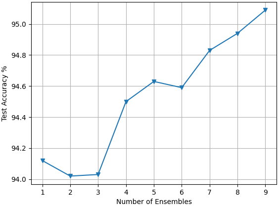
(a) Accuracy

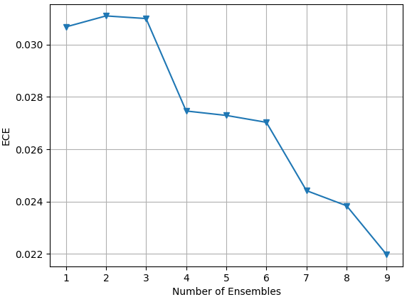
(b) Expected calibration error

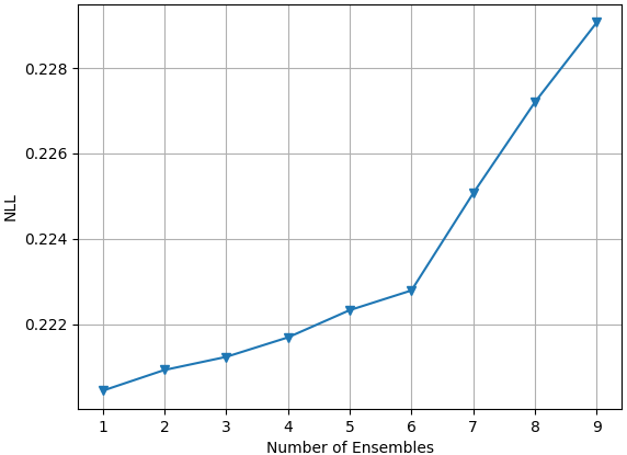
(c) Negative log-likelihood

Figure 2: Accuracy and calibration evaluation metrics as a function of the number of ensembles.

4 Conclusions and Future Work

In this work, we proposed the UraeNAS approach that leverages probabilistic differentiable neural architecture search and approximate Bayesian inference to learn a joint distribution of the architecture and weight parameters in a neural network. Through our experiments with CIFAR-10 for in-distribution data and corrupted CIFAR-10 for out-of-distribution data, we conclude with the following remarks: (1) weight samples/ensemble improves calibration and accuracy compared to (single) deterministic model;(2) architecture samples improve both accuracy and calibration/robustness over the weight ensemble;(3) joint architecture and weight ensemble improve both accuracy and calibration/robustness over deterministic, weight-only ensembles, and architecture-only ensembles.

As a follow-up work, we will compare UraeNAS with other probabilistic weight ensembling approaches Havasi et al. (2021) that improve on naive deep ensembles, as well as deterministic architecture ensembling techniques Egele et al. (2021) to systematically study the computational cost vs. robustness/accuracy trade-off. Furthermore, we will expand the benchmark data and architecture space to study the generalizability of UraeNAS.

5 Acknowledgments

This material is based upon work supported by the US Department of Energy, Office of Science, Office of Fusion Energy Sciences under award DESC0021203, and Advanced Scientific Computing Research through SciDAC Rapids2 under the contract number DE-AC02-06CH11357. We gratefully acknowledge the computing resources provided on Swing, a high-performance computing cluster operated by the Laboratory Computing Resource Center at Argonne National Laboratory.

Appendix A Appendix

Algorithm 1 Unified probabilistic architecture and weight ensembling NAS (UraeNAS)

1:  Inputs: training data $\mathcal{D}_{t}=\{(x_{i},y_{i})\}_{i=1}^{N}$, validation data $\mathcal{D}_{v}=\{(x_{i},y_{i})\}_{i=1}^{N}$, operation candidate space $O$, number of architecture ensembles ($M_{\theta}$), number of weight ensembles ($M_{w}$), model initialization $(\bm{\beta}^{0},\ \bm{w}^{0})$, learning rates $(\eta,\alpha_{0})$, total training epochs $K$, number of cycles $C$, and exploration threshold $r$ for cSGLD.

2:  Method: # Train Phase

3:  for $k=1,2,\dots,K$ do

4:     Update $\bm{\beta}^{(k)}\leftarrow\bm{\beta}^{(k-1)}-\eta\nabla\mathbb{E}_{q(\bm{\theta}|\bm{\beta}^{(k-1)})}\mathcal{L}_{val}(\bm{w}^{(k-1)},\bm{\theta})$

5:      Adjust cyclical learning rate $\alpha_{k}=\frac{\alpha_{0}}{2}\bigg{[}cos(\frac{\pi mod(k-1,\lceil K/C\rceil)}{\lceil K/C\rceil})+1\bigg{]}$

6:     if  $\frac{mod(k-1,[K/M])}{[K/M]}<r$ then

7:        Exploration: $\bm{w}^{(k)}\leftarrow\bm{w}^{(k-1)}-\alpha_{k}\nabla\mathbb{E}_{q(\bm{\theta}|\bm{\beta}^{(k)})}\mathcal{L}_{train}(\bm{w}^{(k-1)},\bm{\theta})$

8:     else

9:        Sampling: $\bm{w}^{(k)}\leftarrow\bm{w}^{(k-1)}-\alpha_{k}\nabla\mathbb{E}_{q(\bm{\theta}|\bm{\beta}^{(k)})}\mathcal{L}_{train}(\bm{w}^{(k-1)},\bm{\theta})+\sqrt{2\alpha_{k}}\epsilon_{k}$,     $\epsilon_{k}\sim N(0,I)$

10:     end if

11:  end for

12:  Store the converged architecture hyper-parameters $\bm{\beta}^{(K)}$. # Evaluation Phase

13:  for $m=1,2,\dots,M_{\theta}$ do

14:     Sample $\bm{\theta}_{m}\stackrel{{\scriptstyle iid}}{{\sim}}\text{Dirichlet}(\bm{\beta}^{(K)})$ to generate model architecture $m$.

15:     for $k=1,2,\dots,(2K)$ do

16:        Update weight parameters $\bm{w}^{(k)}$ using steps 5 to 10.

17:        Store last $\lfloor\frac{M_{w}}{C}\rfloor$ weight parameters $\bm{w}^{(k)}$ in Sampling stage of each cycle.

18:     end for

19:  end for

20:  Load models $\mathcal{M}:(\bm{w},\bm{\theta})_{m},m=1,2,\dots\mathcal{E}$,      $\mathcal{E}\leq M_{w}\times M_{\theta}$ and generate predictions $y_{m}$.

21:  Output: Stored models corresponding to $(\bm{w}_{m_{1}},\bm{\theta}_{m_{2}})$    $1\leq m_{1}\leq M_{w},1\leq m_{2}\leq M_{\theta}$, Ensemble predictions $y_{avg}=\frac{1}{m}\sum_{m=1}^{M}y_{m}$

References

- Hendrycks et al. (2021) Hendrycks, D., Carlini, N., Schulman, J., and Steinhardt, J. (2021), “Unsolved problems in ml safety,” arXiv preprint arXiv:2109.13916.
- Lakshminarayanan et al. (2017) Lakshminarayanan, B., Pritzel, A., and Blundell, C. (2017), “Simple and scalable predictive uncertainty estimation using deep ensembles,” Advances in neural information processing systems, 30.
- Wilson and Izmailov (2020) Wilson, A. G. and Izmailov, P. (2020), “Bayesian deep learning and a probabilistic perspective of generalization,” Advances in neural information processing systems, 33, 4697–4708.
- Jantre et al. (2022) Jantre, S., Madireddy, S., Bhattacharya, S., Maiti, T., and Balaprakash, P. (2022), “Sequential Bayesian Neural Subnetwork Ensembles,” arXiv preprint arXiv:2206.00794.
- Gal and Ghahramani (2016) Gal, Y. and Ghahramani, Z. (2016), “Dropout as a bayesian approximation: Representing model uncertainty in deep learning,” in international conference on machine learning, pp. 1050–1059, PMLR.
- Wan et al. (2013) Wan, L., Zeiler, M., Zhang, S., Le Cun, Y., and Fergus, R. (2013), “Regularization of neural networks using dropconnect,” in International conference on machine learning, pp. 1058–1066, PMLR.
- Singh et al. (2016) Singh, S., Hoiem, D., and Forsyth, D. (2016), “Swapout: Learning an ensemble of deep architectures,” Advances in neural information processing systems, 29.
- Jantre et al. (2021) Jantre, S., Bhattacharya, S., and Maiti, T. (2021), “Layer Adaptive Node Selection in Bayesian Neural Networks: Statistical Guarantees and Implementation Details,” arXiv preprint arXiv:2108.11000.
- Wen et al. (2020) Wen, Y., Tran, D., and Ba, J. (2020), “Batchensemble: an alternative approach to efficient ensemble and lifelong learning,” arXiv preprint arXiv:2002.06715.
- Havasi et al. (2021) Havasi, M., Jenatton, R., Fort, S., Liu, J. Z., Snoek, J., Lakshminarayanan, B., Dai, A. M., and Tran, D. (2021), “Training independent subnetworks for robust prediction,” in 9th International Conference on Learning Representations (ICLR-2021).
- Izmailov et al. (2021) Izmailov, P., Vikram, S., Hoffman, M. D., and Wilson, A. G. G. (2021), “What Are Bayesian Neural Network Posteriors Really Like?” in Proceedings of the 38th International Conference on Machine Learning (ICML-2021), pp. 4629–4640.
- Zoph and Le (2017) Zoph, B. and Le, Q. (2017), “Neural Architecture Search with Reinforcement Learning,” in International Conference on Learning Representations.
- Liu et al. (2018) Liu, C., Zoph, B., Neumann, M., Shlens, J., Hua, W., Li, L.-J., Fei-Fei, L., Yuille, A., Huang, J., and Murphy, K. (2018), “Progressive neural architecture search,” in Proceedings of the European conference on computer vision (ECCV), pp. 19–34.
- Real et al. (2019) Real, E., Aggarwal, A., Huang, Y., and Le, Q. V. (2019), “Regularized evolution for image classifier architecture search,” in Proceedings of the AAAI conference on artificial intelligence, vol. 33, pp. 4780–4789.
- Liu et al. (2019) Liu, H., Simonyan, K., and Yang, Y. (2019), “DARTS: Differentiable Architecture Search,” in International Conference on Learning Representations.
- Chen et al. (2021) Chen, X., Wang, R., Cheng, M., Tang, X., and Hsieh, C.-J. (2021), “Dr{NAS}: Dirichlet Neural Architecture Search,” in International Conference on Learning Representations.
- Zhou et al. (2019) Zhou, H., Yang, M., Wang, J., and Pan, W. (2019), “BayesNAS: A Bayesian Approach for Neural Architecture Search,” in Proceedings of the 36th International Conference on Machine Learning.
- Zhang et al. (2022) Zhang, M., Pan, S., Chang, X., Su, S., Hu, J., Haffari, G. R., and Yang, B. (2022), “BaLeNAS: Differentiable Architecture Search via the Bayesian Learning Rule,” in Proceedings of the IEEE/CVF Conference on Computer Vision and Pattern Recognition, pp. 11871–11880.
- Xie et al. (2019) Xie, S., Zheng, H., Liu, C., and Lin, L. (2019), “SNAS: stochastic neural architecture search,” in International Conference on Learning Representations.
- Dong and Yang (2019) Dong, X. and Yang, Y. (2019), “Searching for a Robust Neural Architecture in Four GPU Hours,” in Proceedings of the IEEE/CVF Conference on Computer Vision and Pattern Recognition (CVPR).
- Zhang et al. (2020) Zhang, R., Li, C., Zhang, J., Chen, C., and Wilson, A. G. (2020), “Cyclical Stochastic Gradient MCMC for Bayesian Deep Learning,” in International Conference on Learning Representations.
- Dong and Yang (2020) Dong, X. and Yang, Y. (2020), “NAS-Bench-201: Extending the Scope of Reproducible Neural Architecture Search,” in International Conference on Learning Representations.
- Hendrycks and Dietterich (2019) Hendrycks, D. and Dietterich, T. (2019), “Benchmarking neural network robustness to common corruptions and perturbations,” in 7th International Conference on Learning Representations (ICLR-2019).
- Egele et al. (2021) Egele, R., Maulik, R., Raghavan, K., Balaprakash, P., and Lusch, B. (2021), “AutoDEUQ: Automated Deep Ensemble with Uncertainty Quantification,” arXiv preprint arXiv:2110.13511.