Unweighted estimation based on optimal sample under measurement constraints

Abstract

To tackle massive data, subsampling is a practical approach to select the more informative data points. However, when responses are expensive to measure, developing efficient subsampling schemes is challenging, and an optimal sampling approach under measurement constraints was developed to meet this challenge. This method uses the inverses of optimal sampling probabilities to reweight the objective function, which assigns smaller weights to the more important data points. Thus the estimation efficiency of the resulting estimator can be improved. In this paper, we propose an unweighted estimating procedure based on optimal subsamples to obtain a more efficient estimator. We obtain the unconditional asymptotic distribution of the estimator via martingale techniques without conditioning on the pilot estimate, which has been less investigated in the existing subsampling literature. Both asymptotic results and numerical results show that the unweighted estimator is more efficient in parameter estimation.

keywords: Generalized Linear Models; Massive Data; Martingale Central Limit Theorem

MSC2020: Primary 62D05; secondary 62J12

NCMIS, KLSC, Academy of Mathematics and Systems Science, CAS, Beijing 100190, China ¹

School of Mathematical Sciences, University of Chinese Academy of Sciences, Beijing 100049, China ²

Department of Statistics, University of Connecticut, Storrs, CT 06269, U.S.A. ³

1 INTRODUCTION

Data acquisition is becoming easier nowadays, and massive data bring new challenges to data storage and processing. Conventional statistical models may not be applicable due to limited computational resources. Facing such problems, subsampling has become a popular approach to reduce computational burdens. The key idea of subsampling is to collect more informative data points from the full data and perform calculations on a smaller data set, see Drineas et al. (2006); Drineas et al. (2011); Mahoney (2011). In some circumstances, covariates $\{X_{i}\}$ are available for all the data points, but responses $\{Y_{i}\}$ can be obtained for only a small portion because they are expensive to measure. For example, the extremely large size of modern galaxy datasets has made visual classification of galaxies impractical. Most subsampling probabilities developed recently for generalized linear models (GLMs) rely on complete responses in the full data set, see Wang et al. (2018); Wang (2019), Ai et al. (2021). In order to handle the difficulty when responses are hard to measure, Zhang et al. (2021) proposed a response-free optimal sampling scheme under measurement constraints (OSUMC) for GLMs. However, their method uses the reweighted estimator which is not the most efficient one, since it assigns smaller weights to the more informative data points in the objective function. The robust sampling probabilities proposed in Nie et al. (2018) do not depend on the responses either, but their investigation focused on linear regression models.

In this paper, we focus on a subsampling method under measurement constraints and propose a more efficient estimator based on the same subsamples taken according to OSUMC for GLMs. We use martingale techniques to derive the unconditional asymptotic distribution of the unweighted estimator and show that its asymptotic covariance matrix is smaller, in the Loewner ordering, than that of the weighted estimator. Before showing the structure of the paper, we first give a short overview of the emerging field of subsampling methods.

Various subsampling methods have been studied in recent years. For linear regression, Drineas et al. (2006) developed a subsampling method based on statistical leveraging scores. Drineas et al. (2011) developed an algorithm using randomized Hardamard transform. Ma et al. (2015) investigated the statistical perspective of leverage sampling. Wang et al. (2019) developed an information-based procedure to select optimal subdata for linear regression deteministically. Zhang & Wang (2021) proposed a distributed sampling-based approach for linear models. Ma et al. (2020) studied the statistical properties of sampling estimators and proposed several estimators based on asymptotic results which are related to leveraging scores. Beyond linear models, Fithian & Hastie (2014) proposed a local case-control subsampling method to handle imbalanced data sets for logistic regression. Wang et al. (2018) developed an optimal sampling method under A-optimality criterion (OSMAC) for logistic regression. Their estimator can be improved because inverse probability reweighting is applied on the objective function, and Wang (2019) developed a more efficient estimator for logistic regression based on optimal subsample. They proposed an unweighted estimator with bias correction using an idea similar to Fithian & Hastie (2014). They also introduced a Poisson sampling algorithm to reduce RAM usage when calculating optimal sampling probabilities. Ai et al. (2021) generalized OSMAC to GLMs and obtained optimal subsampling probabilities under A- and L-optimality criteria for GLMs. These optimal sampling methods require all the responses in order to construct optimal probabilities, which is not possible under measurement constraints. Zhang et al. (2021) developed an optimal sampling method under measurement constraints. Their estimator is also based on the weighted objective function and thus the performance can be improved. Recently, Cheng et al. (2020) extended an information-based data selection approach for linear models to logistic regression. Yu et al. (2022) derived optimal Poisson subsampling probabilies under the A- and L-optimality criteria for quasi-likelihood estimation, and developed a distributed subsampling framwork to deal with data stored in different machines. Wang & Ma (2020) developed an optimal sampling method for quantile regression. Pronzato & Wang (2021) proposed a sequential online subsampling procedure based on optimal bounded design measures.

We focus on GLMs in this paper, which include commonly used models such as linear, logistic and Poisson regression. The rest of the paper is organized as follows. Section 2 presents the model setup and briefly reviews the OSUMC method. The more efficient estimator and its asymptotic properties are presented in Section 3. Section 4 provides numerical simulations. We summarize our paper in Section 5. Proofs and technical details are presented in the Supplementary Material.

2 BACKGROUND AND MODEL SETUP

We start by reviewing GLMs. Consider independent and identically distributed (i.i.d) data $(X_{1},Y_{1})$, $(X_{2},Y_{2})$,…, $(X_{n},Y_{n})$ from the distribution of $(X,Y)$, where $X\in\mathbb{R}^{p}$ is the covariate vector and $Y$ is the response variable. Assume that the conditional density of $Y$ given $X$ satisfies that

$$f(y|x,\beta_{0},\sigma)\propto\exp\left\{\frac{yx^{T}\beta_{0}-b(x^{T}\beta_{0})}{c(\sigma)}\right\},$$

where $\beta_{0}$ is the unknown parameter we need to estimate from data, $b(\cdot)$ and $c(\cdot)$ are known functions, and $\sigma$ is the dispersion parameter. In this paper, we are only interested in estimating $\beta_{0}$. Thus, we take $c(\sigma)=1$ without loss of generality. We also include an intercept in the model, as is almost always the case in practice. We obtain the maximum likelihood estimator (MLE) of $\beta_{0}$ through maximizing the loglikelihood function, namely,

$$\hat{\beta}_{\text{MLE}}:=\mathop{\arg\max}_{\beta}\frac{1}{n}\sum_{i=1}^{n}\left\{Y_{i}X_{i}^{T}\beta-b(X_{i}^{T}\beta)\right\},$$ (1)

which is the same as solving the following score equation:

$$\Psi_{n}(\beta):=\frac{1}{n}\sum_{i=1}^{n}\{b^{{}^{\prime}}(X_{i}^{T}\beta)-Y_{i}\}X_{i}=0,$$

where $b^{{}^{\prime}}(\cdot)$ is the derivative of $b(\cdot)$. There is no general closed-form solution to $\hat{\beta}_{\text{MLE}}$, and iterative algorithms such as Newton’s method are often used. Therefore, when the data are massive, the computational burden of estimating $\beta_{0}$ is very heavy. To handle this problem, Ai et al. (2021) proposed a subsampling-based approach, which constructs sampling probabilities $\{\pi_{i}\}_{i=1}^{n}$ that depend on both the covariates $\{X_{i}\}$ and the responses $\{Y_{i}\}$. However, it is infeasible to obtain all the responses under measurement constraints. For example, it costs considerable money and time to synthesize superconductors. When we use data-driven methods to predict the critical temperature with the chemical composition of superconductors, it may be more pratical to measure a small number of materials to build a data-driven model. To tackle this type of “many $X$, few $Y$” scenario, Zhang et al. (2021) developed OSUMC subsampling probabilities.

Assume we obtain a subsample of size $r$ by sampling with replacement according to the probabilities $\pi=\{\pi_{i}\}_{i=1}^{n}$. A reweighted estimator is often used in subsample literature, defined as the minimizer of the reweighted target function, namely

$$\hat{\beta}_{\mathrm{w}}:=\mathop{\arg\max}_{\beta}\frac{1}{r}\sum_{i=1}^{r}\frac{Y_{i}^{*}X_{i}^{*{T}}\beta-b(X_{i}^{*{T}}\beta)}{n\pi_{i}^{*}},$$ (2)

where $(X_{i}^{*},Y_{i}^{*})$ is the data sampled in the $i$th step, and $\pi_{i}^{*}$ denotes the corresponding sampling probability. Equivalently, we can solve the reweighted score function

$$\Psi^{*}_{\mathrm{w}}(\beta):=\frac{1}{r}\sum_{i=1}^{r}\frac{b^{{}^{\prime}}(X_{i}^{*{T}}\beta)-Y_{i}^{*}}{n\pi_{i}^{*}}X_{i}^{*}=0,$$

to obtain the reweighted estimator. Zhang et al. (2021) proposed a scheme to derive the optimal subsampling probabilities for GLMs under measurement constraints. They first proved that $\hat{\beta}_{\mathrm{w}}$ is asymptotically normal:

$$\mathbb{V}\{\Psi^{*}_{\mathrm{w}}(\beta_{0})\}^{-\frac{1}{2}}\Phi(\hat{\beta}_{\mathrm{w}}-\beta_{0})\xrightarrow{d}N(0,I),$$

where the notation “$\xrightarrow{d}$” denotes convergence in distribution,

$$\mathbb{V}\{\Psi^{*}_{\mathrm{w}}(\beta_{0})\}:=\mathbb{E}\left[\mathbb{V}\{\Psi^{*}_{\mathrm{w}}(\beta_{0})|X_{1}^{n}\}\right]=\mathbb{E}\left\{\frac{1}{n^{2}}\sum_{i=1}^{n}b^{{}^{\prime\prime}}(X_{i}^{T}\beta_{0})X_{i}X_{i}^{T}\left(\frac{1}{r\pi_{i}}-\frac{1}{r}+1\right)\right\},$$

$X_{1}^{n}:=(X_{1},X_{2},...,X_{n})$, $b^{{}^{\prime\prime}}(\cdot)$ is the second derivative of $b(\cdot)$, and

$$\Phi:=\mathbb{E}\left\{\frac{1}{n}\sum_{i=1}^{n}b^{{}^{\prime\prime}}(X_{i}^{T}\beta_{0})X_{i}X_{i}^{T}\right\}.$$ (3)

Since the matrix $\Phi^{-1}\mathbb{V}\{\Psi^{*}_{\mathrm{w}}(\beta_{0})|X_{1}^{n}\}\Phi^{-1}$ converges to the asymptotic variance of $\hat{\beta}_{\mathrm{w}}$, Zhang et al. (2021) minimized its trace, $\text{tr}(\Phi^{-1}\mathbb{V}\{\Psi^{*}_{\mathrm{w}}(\beta_{0})|X_{1}^{n}\}\Phi^{-1})$, to obtain the optimal sampling probabilities which depend only on covariate vectors $X_{1}$ ,…, $X_{n}$:

$$\pi_{i}^{\mathrm{A-OS}}(\beta_{0},\Phi)=\frac{\sqrt{b^{{}^{\prime\prime}}(X_{i}^{T}\beta_{0})}\|\Phi^{-1}X_{i}\|}{\sum_{j=1}^{n}\sqrt{b^{{}^{\prime\prime}}(X_{j}^{T}\beta_{0})}\|\Phi^{-1}X_{j}\|}.$$ (4)

To avoid the matrix multiplication in $\|\Phi^{-1}X_{i}\|$ in (4), we can consider a variant of (4) which omits the inverse matrix $\Phi^{-1}$:

$$\pi_{i}^{\mathrm{L-OS}}(\beta_{0})=\frac{\sqrt{b^{{}^{\prime\prime}}(X_{i}^{T}\beta_{0})}\|X_{i}\|}{\sum_{j=1}^{n}\sqrt{b^{{}^{\prime\prime}}(X_{j}^{T}\beta_{0})}\|X_{j}\|}.$$ (5)

Here, $\{\pi_{i}^{\mathrm{L-OS}}\}_{i=1}^{n}$ are other widely used optimal probabilities, derived by minimizing the quantity $\text{tr}(L\Phi^{-1}\mathbb{V}\{\Psi^{*}_{\mathrm{w}}(\beta_{0})|X_{1}^{n}\}\Phi^{-1}L^{T})$ with $L=\Phi$. This is a special case of using the L-optimality criterion to obtain optimal subsampling probabilities (see Wang et al., 2018; Ai et al., 2021). The probabilities in (4) and (5) are useful when the responses are not available, as we discussed before. However, as pointed out in Wang (2019), under the logistic model framework, the weighting scheme adopted in (2) does not bring us the most efficient estimator. Intuitively, if a data point $(X_{i},Y_{i})$ has a larger sampling probability, it contains more information about $\beta_{0}$. However, data points with higher sampling probabilities have smaller weights in (2). This will reduce the efficiency of the estimator. We propose a more efficient estimator based on the unweighted target function.

3 UNWEIGHTED ESTIMATION AND ASYMPTOTIC THEORY

In this section, we present an algorithm with an unweighted estimator and derive its asymptotic property. As we discussed before, the reweighted estimator reduces the importance of more informative data points. To overcome this problem, Wang (2019) developed a method to correct the bias of the unweighted estimator in logistic regression. In this section, we show that, using the optimal probabilities under measurement constraints, the unweighted estimator is asymptotically unbiased and therefore it is a better estimator since it has a smaller asymptotic variance matrix in the Loewner ordering. To make our investigation more general and put the probabilities in (4) and (5) in an unified class, we consider the following general class of subsampling probabilities in the rest of the paper:

$$\pi_{i}^{\mathrm{OS}}(\beta_{0},\Phi)=\frac{\sqrt{b^{{}^{\prime\prime}}(X_{i}^{T}\beta_{0})}\|L\Phi^{-1}X_{i}\|}{\sum_{j=1}^{n}\sqrt{b^{{}^{\prime\prime}}(X_{j}^{T}\beta_{0})}\|L\Phi^{-1}X_{j}\|},$$ (6)

where $L$ is a fixed matrix. Here the probabilities $\{\pi_{i}^{\mathrm{OS}}(\beta_{0},\Phi)\}_{i=1}^{n}$ are optimal in that they minimize the asymptotic variance of $L\hat{\beta}_{\mathrm{w}}$. Specifically, when $L=I$, the probabilities in (6) reduce to those in (4) and when $L=\Phi$, they reduce to those in (5).

We define our unweighted estimator as:

$$\hat{\beta}_{\mathrm{uw}}:=\mathop{\arg\max}_{\beta}\frac{1}{r}\sum_{i=1}^{r}\left\{Y_{i}^{*}X_{i}^{*{T}}\beta-b(X_{i}^{*{T}}\beta)\right\},$$ (7)

where $(X_{i}^{*},Y_{i}^{*})$’s are sampled according to the probabilities in (6).

3.1 Notation and main algorithm

We first introduce some notations and the main algorithm. Recall that $X_{1}^{n}:=(X_{1},X_{2},...,X_{n})$ and denote $Y_{1}^{n}:=(Y_{1},Y_{2},...,Y_{n})$. For a vector $X\in\mathbb{R}^{p}$, we use $\|X\|$ to denote its Euclidean norm. For a matrix $A\in\mathbb{R}^{p\times p}$, we use $\lambda_{\min}(A)$ and $\lambda_{\max}(A)$ to denote its minimum and maxmum eigenvalues, respectively, $\|A\|_{F}$ to denote its Frobenius norm, and $\text{tr}(A)$ to denote its trace. For two positive semi-definite matrices $A$ and $B$, $A\geq B$ if and only if $A-B$ is positive semi-definite; this is known as the Loewner ordering. For parameter $\beta$, we assume that $\beta$ takes values in a compact set $\beta\in\mathbb{B}$. Now, we present the main algorithm in Algorithm 1. Since the probabilities in (6) involve unknown quantities, $\beta_{0}$ and $\Phi$, we use pilot estimates to replace them in Algorithm 1.

Algorithm 1 Unweighted estimation for GLM under measurement constraints

1:  Take a pilot subsample of size $r_{\mathrm{p}}$: $\{(X_{i}^{*_{\mathrm{p}}},Y_{i}^{*_{\mathrm{p}}})\}_{i=1}^{r_{\mathrm{p}}}$ with simple random sampling from the full data set $\{(X_{i},Y_{i})\}_{i=1}^{n}$. Calculate the pilot estimate of $\beta_{0}$:

$$\hat{\beta}_{\mathrm{p}}:=\mathop{\arg\max}_{\beta}\frac{1}{r_{\mathrm{p}}}\sum_{i=1}^{r_{\mathrm{p}}}\left\{Y_{i}^{*_{\mathrm{p}}}X_{i}^{*_{\mathrm{p}}{T}}\beta-b(X_{i}^{*_{\mathrm{p}}{T}}\beta)\right\},$$

and the pilot estimate of $\Phi$:

$$\hat{\Phi}_{\mathrm{p}}:=\frac{1}{r_{\mathrm{p}}}\sum_{i=1}^{r_{\mathrm{p}}}b^{{}^{\prime\prime}}(X_{i}^{*_{\mathrm{p}}{T}}\hat{\beta}_{\mathrm{p}})X_{i}^{*_{\mathrm{p}}}X_{i}^{*_{\mathrm{p}}{T}}.$$

2:  Use $\hat{\beta}_{\mathrm{p}}$ and $\hat{\Phi}_{\mathrm{p}}$ to replace $\beta_{0}$ and $\Phi$ in (6), respectively, and calculate the sampling probabilities $\{\pi_{i}^{\mathrm{OS}}(\hat{\beta}_{\mathrm{p}},\hat{\Phi}_{\mathrm{p}})\}_{i=1}^{n}$.

3:  Obtain a subsample $\{(X_{i}^{*},Y_{i}^{*})\}_{i=1}^{r}$ of size $r$ according to the sampling probabilities $\{\pi_{i}^{\mathrm{OS}}(\hat{\beta}_{\mathrm{p}},\hat{\Phi}_{\mathrm{p}})\}_{i=1}^{n}$ using sampling with replacement, and solve the estimation equation:

$$\Psi_{\mathrm{uw}}^{*}(\beta):=\frac{1}{r}\sum_{i=1}^{r}\{b^{{}^{\prime}}(X_{i}^{*{T}}\beta)-Y_{i}^{*}\}X_{i}^{*}=0,$$

to obtain the unweighted estimator defined in (7).

Remark 1.

Our Algorithm 1 is different from the subsampling algorithm in Zhang et al. (2021) at step 3 of obtaining the subsampling estimators. There are two types of weights in the subsampling algorithms: one is the sampling weights which we call subsampling probabilities in this paper, and the other is the estimation weights used to construct the target function. Algorithm 1 and Zhang et al. (2021)’s algorithm share the same sampling probabilities (sampling weights) but they use different estimation weights. Zhang et al. (2021) use the estimation weights $1/\pi_{i}^{\mathrm{OS}}(\hat{\beta}_{\mathrm{p}},\hat{\Phi}_{\mathrm{p}})$ while we set the estimation weights to be uniformly one, i.e., the target function is unweighted. We will show in Section 3.3 that our estimator improves the estimation efficiency. This does not contradict the fact that $\{\pi_{i}^{\mathrm{OS}}\}_{i=1}^{n}$ are optimal for the algorithm in Zhang et al. (2021), because they force the estimation weights to be the inverses of the sampling weights while we do not enforce this requirement.

Remark 2.

The computational complexity of our two-step Algorithm 1 is the same as the OSUMC estimator in Zhang et al. (2021), because we use the same sampling probabilities and the two methods differ only in the weights of the target function. With Newton’s method, it requires $O(\zeta_{\mathrm{p}}r_{\mathrm{p}}p^{2})$ time to compute the pilot estimates, where $\zeta_{\mathrm{p}}$ is the number of iterations for the algorithm to convergence based on the pilot sample. The time complexities of calculating sampling probabilities $\{\pi^{\mathrm{A-OS}}\}_{i=1}^{n}$ and $\{\pi^{\mathrm{L-OS}}\}_{i=1}^{n}$ are $O(np^{2})$ and $O(np)$, respectively. After obtaining the second stage subsample with the optimal sampling probabilities, it takes $O(\zeta rp^{2})$ time to solve the unweighted target function where $\zeta$ is the number of iterations of Newton’s algorithm. Thus, the total computational time is $O(np^{2}+\zeta_{\mathrm{p}}r_{\mathrm{p}}p^{2}+\zeta rp^{2})$ for A-optimality and $O(np+\zeta_{\mathrm{p}}r_{\mathrm{p}}p^{2}+\zeta rp^{2})$ for L-optimality. The computational complexity of our algorithm based on the A-optimality criterion is the same as the OSUMC algorithm in Zhang et al. (2021). Therefore, our method increase the estimation efficiency without increasing the computational burden.

3.2 Asymptotic normality of $\hat{\beta}_{\mathrm{uw}}$

We focus on unconditional asymptotic results for the unweighted algorithm, and use martingale techniques to prove theorems. To present the asymptotic results, we summarize some regularity conditions first.

Assumption 1.

The second derivative $b^{{}^{\prime\prime}}(\cdot)$ is bounded and continuous.

Assumption 2.

The fourth moment of the covariate is finite, i.e., $\mathbb{E}\left(\|X\|^{4}\right)<\infty$.

Assumption 3.

Let $g(x):=\inf_{\beta\in\mathbb{B}}b^{{}^{\prime\prime}}(x^{T}\beta)$. Assume that $\lambda_{\min}[\mathbb{E}\{g(X)XX^{T}\}]>0$. Assume that there exists a function $h(x)$ such that $|b^{{}^{\prime\prime\prime}}(x^{T}\beta)|\leq h(x)$ and $\mathbb{E}\{h(X)\|X\|^{4}\}<\infty$, where $b^{{}^{\prime\prime\prime}}(\cdot)$ denotes the third derivative of $b(\cdot)$.

Assumption 1 is commonly used in GLM literature, e.g., Zhang et al. (2021). Assumption 2 is a moment condition on $X$. The second part of Assumption 3 is similar to the third-derivative condition used in the classical theory of MLE. However, here we need a stronger moment condition, $\mathbb{E}[h(X)\|X\|^{4}]<\infty$, since we use an unequal probability sampling method. Before we prove the asymptotic normality of $\hat{\beta}_{\mathrm{uw}}$, we need to prove some lemmas. First, we present the convergence of $\dot{\Psi}_{\mathrm{uw}}^{*}(\beta)$.

Lemma 1.

Under assumptions A1-A3, for every sequence $\beta_{n}\xrightarrow{p}\beta_{0}$,

$$\hat{m}\dot{\Psi}_{\mathrm{uw}}^{*}(\beta_{n})\xrightarrow{p}\Gamma:=\mathbb{E}\left[\left\{b^{{}^{\prime\prime}}(X^{T}\beta_{0})\right\}^{\frac{3}{2}}\|L\Phi^{-1}X\|XX^{T}\right],$$

where $\hat{m}=(1/n)\sum_{i=1}^{n}\sqrt{b^{{}^{\prime\prime}}(X_{i}^{T}\hat{\beta}_{\mathrm{p}})}\|L\hat{\Phi}_{\mathrm{p}}^{-1}X_{i}\|$ and the notation “$\xrightarrow{p}$” denotes convergence in probability.

Furthermore, to establish the asymptotic normality of $\hat{\beta}_{\mathrm{uw}}$, we present the asymptotic normality of $\Psi_{\mathrm{uw}}^{*}(\beta_{0})$.

Lemma 2.

Under assumptions A1-A3, if $r/n\to\rho\in[0,1)$, $r_{\mathrm{p}}/\sqrt{n}\to 0$ and $\exists\delta>0$ such that

$$\mathbb{E}\left\{\left|b^{{}^{\prime}}(X^{T}\beta_{0})-Y\right|^{4+2\delta}\left\|X\right\|^{8+4\delta}\right\}<\infty,$$ (8)

then

$$\sqrt{r}\hat{m}\Psi_{\mathrm{uw}}^{*}(\beta_{0})\xrightarrow{d}N(0,m\Gamma+\rho\Omega),$$

where $m:=\mathbb{E}\left\{\sqrt{b^{{}^{\prime\prime}}(X^{T}\beta_{0})}\|L\Phi^{-1}X\|\right\}$ and $\Omega=\mathbb{E}\left[\left\{b^{{}^{\prime\prime}}(X^{T}\beta_{0})\right\}^{2}\|L\Phi^{-1}X\|^{2}XX^{T}\right]$. If specifically $\rho=0$, then the required condition in (8) can be weakened to

$$\mathbb{E}\left\{\left|b^{{}^{\prime}}(X^{T}\beta_{0})-Y\right|^{2+\delta}\left\|X\right\|^{4+2\delta}\right\}<\infty.$$

We will use the central limit theorem for martingales described in Jakubowski (1980) and Zhang et al. (2021) to prove this Lemma in the supplementary material. In Algorithm 1, the pilot subsample and the optimal subsample are from the same full data so the unconditional distributions of the two subsamples are not independent and it is possible to have overlaps. The assumption $r_{\mathrm{p}}/\sqrt{n}\to 0$ is to ensure that the data points used in the pilot subsample are asymptotically negligible when deriving the unconditional asymptotic distribution of $\Psi_{\mathrm{uw}}^{*}(\beta_{0})$ which depends on both subsamples. This assumption can be replaced by other alternatives such as assuming that the pilot estimator is independent of the full data (e.g., Fithian & Hastie, 2014) and this is appropriate if we modify step 3 of Algorithm 1 to sample from the rest of the data with the pilot subsample data points removed.

Now, we are ready to show the asymptotic normality of the unweighted estimator.

Theorem 1.

Under assumptions A1-A3, assuming that $\Gamma$ is positive-definite, we have

$$\hat{\beta}_{\mathrm{uw}}-\beta_{0}=-\Gamma^{-1}\hat{m}\Psi_{\mathrm{uw}}^{*}(\beta_{0})+o_{p}\left(1/\sqrt{r}\right).$$

In addition, under the conditions of Lemma 2

$$\sqrt{r}(\hat{\beta}_{\mathrm{uw}}-\beta_{0})\xrightarrow{d}N(0,\Sigma_{\mathrm{uw}}^{\rho}),$$

where

$$\Sigma_{\mathrm{uw}}^{\rho}:=m\Gamma^{-1}+\rho\Gamma^{-1}\Omega\Gamma^{-1}.$$ (9)

Theorem 1 shows that $\hat{\beta}_{\mathrm{uw}}$ is asymptotically unbiased, and from (9) we see that the asymptotic variance of $\hat{\beta}_{\mathrm{uw}}$ can be split into two parts, $m\Gamma^{-1}$ and $\rho\Gamma^{-1}\Omega\Gamma^{-1}$. Here, $m\Gamma^{-1}$ is the contribution from the randomness of subsampling and $\rho\Gamma^{-1}\Omega\Gamma^{-1}$ is due to the randomness of the full data. If the subsample size $r$ is of a smaller order than the full data sample size $n$, i.e., $\rho=0$, then the randomness of the full data is negligible. If $r$ is of the same order as $n$, we need a stronger moment condition (as stated in Lemma 2) to establish asymptotic normality. In the subsampling setting, we usually expect $r\ll n$, and therefore $m\Gamma^{-1}$ is the dominating term of the asymptotic variance of $\hat{\beta}_{\mathrm{uw}}$.

To estimate the asymptotic variance of $\hat{\beta}_{\mathrm{uw}}$, we propose the following formulas involving only the selected subsample:

$$\hat{\mathbb{V}}(\hat{\beta}_{\mathrm{uw}})=\frac{1}{r}\hat{m}\hat{\Gamma}^{-1}+\frac{1}{n}\hat{\Gamma}^{-1}\hat{\Omega}\hat{\Gamma}^{-1},$$ (10)

where

$$\hat{\Gamma}=\frac{\hat{m}}{r}\sum_{i=1}^{r}b^{{}^{\prime\prime}}(X_{i}^{*{T}}\hat{\beta}_{\mathrm{uw}})X_{i}^{*}X_{i}^{*{T}},$$

and

$$\hat{\Omega}=\frac{n\hat{m}^{2}}{r}\sum_{i=1}^{r}\pi_{i}^{*}b^{{}^{\prime\prime}}(X_{i}^{*{T}}\hat{\beta}_{\mathrm{uw}})X_{i}^{*}X_{i}^{*{T}}.$$

Our estimator of the asymptotic variance follows the similar idea that is described in Wang et al. (2018) and Wang (2019).

3.3 Efficiency of the unweighted estimator

In this section, we compare the efficiency of the unweighted estimator $\hat{\beta}_{\mathrm{uw}}$ with the weighted estimator $\hat{\beta}_{\mathrm{w}}$ defined in (2). We first restate the asymptotic result in Zhang et al. (2021). In their paper, they proved that under some regularity conditions, $\hat{\beta}_{\mathrm{w}}$ is asymptotically normal

$$\mathbb{V}\{\Psi^{*}_{\mathrm{w}}(\beta_{0})\}^{-\frac{1}{2}}\Phi(\hat{\beta}_{\mathrm{w}}-\beta_{0})\xrightarrow{d}N(0,I),$$

where

$$\mathbb{V}\{\Psi^{*}_{\mathrm{w}}(\beta_{0})\}=\mathbb{E}\left[\frac{1}{n^{2}}\sum_{i=1}^{n}b^{{}^{\prime\prime}}(X_{i}^{T}\beta_{0})X_{i}X_{i}^{T}\left\{\frac{1}{r\pi_{i}}-\frac{1}{r}+1\right\}\right].$$

Denote

$$\Lambda:=\mathbb{E}\left\{\frac{b^{{}^{\prime\prime}}(X^{T}\beta_{0})XX^{T}}{\sqrt{b^{{}^{\prime\prime}}(X^{T}\beta_{0})}\|L\Phi^{-1}X\|}\right\},$$

and replace $\pi=\{\pi_{i}\}_{i=1}^{n}$ in $\mathbb{V}\{\Psi^{*}_{\mathrm{w}}(\beta_{0})\}$ with the optimal sampling probabilities defined in (6). We then have that

$$\mathbb{V}\{\Psi^{*}_{\mathrm{w}}(\beta_{0})\}=\frac{1}{r}{\frac{n-1}{n}}m\Lambda+\frac{1}{n}\Phi,$$ (11)

where $m$ is defined in Lemma 2 and $\Phi$ is defined in (3). The details of the calculation are presented in the supplementary material. From (11), if $r/n\to\rho$, the asymptotic variance of $\sqrt{r}(\hat{\beta}_{\mathrm{w}}-\beta_{0})$ is

$$\Sigma_{\mathrm{w}}^{\rho}:=m\Phi^{-1}\Lambda\Phi^{-1}+\rho\Phi^{-1}.$$ (12)

The asymptotic variance $\Sigma_{\mathrm{w}}^{\rho}$ consists of two parts: the term $m\Phi^{-1}\Lambda\Phi^{-1}$ is due to the randomness of subsampling while the term $\rho\Phi^{-1}$ is due to the randomness of the full data. Similarly, in the asymptotic variance $\Sigma_{\mathrm{uw}}^{\rho}$ defined in (9) for the unweighted estimator, $m\Gamma^{-1}$ is due to the randomness of subsampling and $\rho\Gamma^{-1}\Omega\Gamma^{-1}$ is due to the randomness of the full data. We have the following results comparing the aforementioned terms for the weighted and unweighted estimators.

Theorem 2.

If $\Phi$, $\Gamma$ and $\Lambda$ are finite and positive-definite, then

$$\Gamma^{-1}\leq\Phi^{-1}\Lambda\Phi^{-1},\quad and\quad\Gamma^{-1}\Omega\Gamma^{-1}\geq\Phi^{-1},$$

where the inequalities are in the Loewner ordering.

From Theorem 2, $m\Gamma^{-1}\leq m\Phi^{-1}\Lambda\Phi^{-1}$. Thus, compared with the weighted estimator, the unweighted estimator has a smaller asymptotic variance component from the randomness of subsampling. On the other hand, since $\rho\Gamma^{-1}\Omega\Gamma^{-1}\geq\rho\Phi^{-1}$, the asymptotic variance component due to the full data randomness is larger for the unweighted estimator. A major motivation of subsampling is to reduce the computational or data measurement cost significantly, so it is typical that $r\ll n$ and therefore $\rho$ is typically very small. In this scenario, the asymptotic variance component due to subsampling is the dominating term, and the unweighted estimator has a higher estimation efficiency than the weighted estimator. In the case that $r/n\to 0$, the asymptotic variance component due to full data randomness is negligible.

We can also get some insights on the difference between the weighted and unweighted estimators by considering them conditionally on the full data. Given the full data, the subsample weighted estimator $\hat{\beta}_{\mathrm{w}}$ is asymptotically unbiased for the full data unweighted MLE $\hat{\beta}_{\text{MLE}}$ in (1), while the subsample unweighted estimator $\hat{\beta}_{\mathrm{uw}}$ is asymptotically unbiased for the full data weighted MLE defined as

$$\hat{\beta}_{\text{wMLE}}:=\mathop{\arg\max}_{\beta}\frac{1}{n}\sum_{i=1}^{n}{w_{i}}\left\{Y_{i}X_{i}^{T}\beta-b(X_{i}^{T}\beta)\right\},$$

where $w_{i}=\sqrt{b^{{}^{\prime\prime}}(X_{i}^{T}\beta_{0})}\|L\Phi^{-1}X_{i}\|$ does not depend on the $\{Y_{i}\}$. Here, $\hat{\beta}_{\text{wMLE}}$ is asymptotically unbiased for the true parameter because the weights $\{w_{i}\}$ are only related to the $\{X_{i}\}$. We see that $\hat{\beta}_{\mathrm{w}}$ and $\hat{\beta}_{\mathrm{uw}}$ essentially approximate different full data estimators $\hat{\beta}_{\text{MLE}}$ and $\hat{\beta}_{\text{wMLE}}$, respectively. It is well known that $\hat{\beta}_{\text{MLE}}$ is more efficient than $\hat{\beta}_{\text{wMLE}}$ based on the full data, but its variation is much smaller than that of $\hat{\beta}_{\mathrm{w}}$ or $\hat{\beta}_{\mathrm{uw}}$, and it is negligible if $r/n\rightarrow 0$. Thus the variation of $\hat{\beta}_{\mathrm{w}}$ around $\hat{\beta}_{\text{MLE}}$ and the variation of $\hat{\beta}_{\mathrm{uw}}$ around $\hat{\beta}_{\text{wMLE}}$ are the major components of the asymptotic variances of $\hat{\beta}_{\mathrm{w}}$ and $\hat{\beta}_{\mathrm{uw}}$ in terms of estimating the true parameter.

When the model is correctly specified, then $\hat{\beta}_{\mathrm{w}}$ and $\hat{\beta}_{\mathrm{uw}}$ are consistent for the same true parameter. However, if the model is misspecified, then $\hat{\beta}_{\mathrm{w}}$ and $\hat{\beta}_{\mathrm{uw}}$ will typically converge to different limits. Heuristically, $\hat{\beta}_{\mathrm{w}}$ will converge to the solution of $\mathbb{E}[X\{Y-b^{{}^{\prime}}(X^{T}\beta)\}]$ while $\hat{\beta}_{\mathrm{uw}}$ will converge to the solution of $\mathbb{E}[wX\{Y-b^{{}^{\prime}}(X^{T}\beta)\}]$ with $w=\sqrt{b^{{}^{\prime\prime}}(X^{T}\beta_{0})}\|L\Phi^{-1}X\|$. In this scenario, it is difficult to compare the efficiency of $\hat{\beta}_{\mathrm{w}}$ with that of $\hat{\beta}_{\mathrm{uw}}$, because it is unknown which solution is closer to the true data-generating parameter.

4 NUMERICAL RESULTS

We investigate the efficiency of the unweighted estimator in parameter estimation through numerical experiments in this section. We present simulation results in Section 4.1 and experiments for real data in Section 4.2.

4.1 Simulation Results

In this section, we use simulations to evaluate the performance of the more efficient estimator we proposed. To compare with the original OSUMC estimator, we use the same setups as described in Section 5 and in the appendix of Zhang et al. (2021), and show numerical results for logistic, Poisson and linear regressions.

4.1.1 Logistic Regression and Poisson regression

We first present simulations for logistic regression for which the conditional density of the response has the form

$$f(y|x,\beta_{0})=\exp\left\{yx^{T}\beta_{0}-\log(1+e^{x^{T}\beta_{0}})\right\},\text{ for }y=0,1.$$

This model implies that the probability of $Y=1$ given $X$ is

$$P(Y=1|X,\beta_{0})=\frac{e^{X^{T}\beta_{0}}}{1+e^{X^{T}\beta_{0}}}.$$

To generate the full data, we set the true parameter $\beta_{0}$ as a 20 dimensional vector with all entries equal to 1. The full data sample size is $n=100,000$ and four distributions of $X$ are considered, which are exactly the same distributions used in Zhang et al. (2021). We present these four covariate distributions below for completeness:

1. mzNormal: The covariate $X$ follows a multivariate normal distribution $N(0,\Sigma)$, where $\Sigma_{ij}=0.5^{I{(i\neq j)}}$ and $I(\cdot)$ represents the indicator function. We have almost equal numbers of 1’s and 0’s in this scenario.

2. nzNormal: The covariate $X$ follows a multivariate normal distribution $N(0.5,\Sigma)$, where $\Sigma$ is defined in mzNormal. In this scenario, roughly 75% of the responses are 1’s.

3. unNormal: The covariate $X$ follows a multivariate normal distribution $N(0,\Sigma_{1})$, where $\Sigma_{1}=U_{1}\Sigma U_{1}$, $U_{1}=diag(1,1/2,...,1/20)$ and $\Sigma$ is the same covariance matrix as we used in mzNormal. For this case, the components of $X$ have different variances.

4. mixNormal: The covariate $X$ follows a mixed multivariate normal distribution, namely, $X\sim 0.5N(0.5,\Sigma)+0.5N(-0.5,\Sigma)$, where $\Sigma$ is the same as what we used in mzNormal.

To compare the performance of the new estimator with the weighted one, we use the empirical MSE of $\hat{\beta}$:

$$\text{eMSE}(\hat{\beta})=\frac{1}{S}\sum_{s=1}^{S}\|\hat{\beta}^{(s)}-\beta_{0}\|.$$ (13)

Here, $\hat{\beta}^{(s)}$ is the estimated parameter we obtained in the $s$-th repetition of the simulation. We repeated the simulation for $S=500$ times to calculate $\text{eMSE}(\hat{\beta})$. For the pilot estimate, we used $r_{\mathrm{p}}=500$ for both weighted and unweighted methods. In every repetition, we generated the full data, which means we focus on the unconditional empirical MSE. Figure 1 shows that our unweighted estimator performs better than the original OSUMC weighted estimator under each setting when applied to logistic regression. This is true for both A-optimality and L-optimality criteria. For instance, when $X$ has a mixNormal distribution, the emprical MSE of the weighted estimator is over 1.15 times as large as that of the unweighted one. In most cases, $\pi_{i}^{\mathrm{A-OS}}$ and $\pi_{i}^{\mathrm{L-OS}}$ perform similarly. When $X$ has a unNormal design, $\pi_{i}^{\mathrm{A-OS}}$ performs significantly better than $\pi_{i}^{\mathrm{L-OS}}$ because the A-optimality aims to directly minimize asymptotic MSE.

To evaluate the performance of (10) in estimating the asymptotic variance, we compare $\text{tr}\{\hat{\mathbb{V}}(\hat{\beta}_{\mathrm{uw}})\}$ with the empirical variance. Figure 2 shows that the estimated variances are very close to the empirical variances under the logistic regression model.

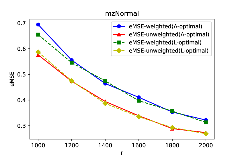
(a) mzNormal

(b) nzNormal

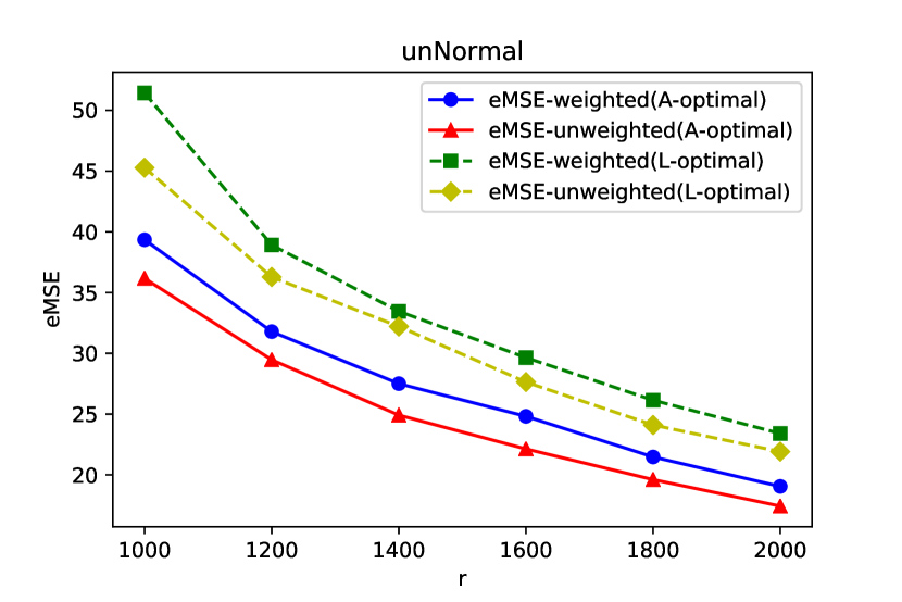
(c) unNormal

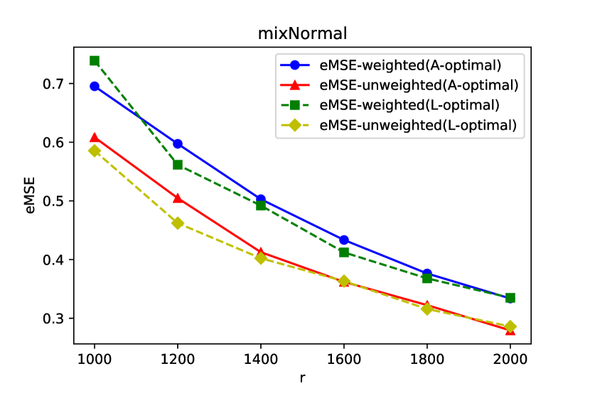
(d) mixNormal

Figure 1: eMSE for different subsample sizes $r$ with a pilot sample size $r_{\mathrm{p}}=500$ for logistic regression under different settings.

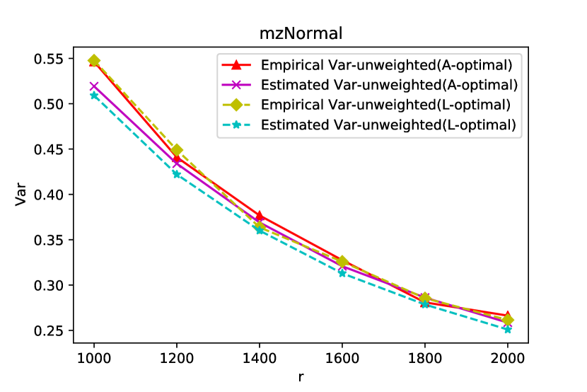
(a) mzNormal

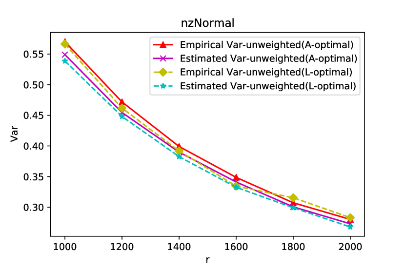
(b) nzNormal

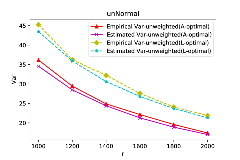
(c) unNormal

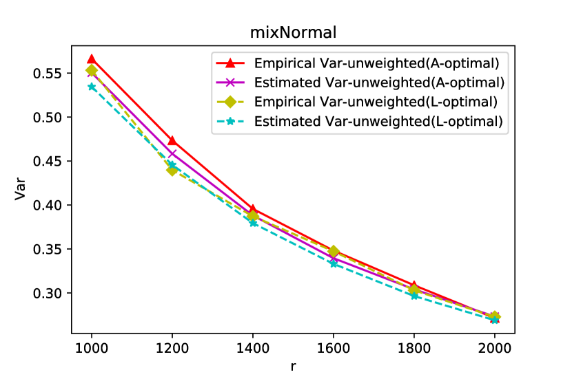
(d) mixNormal

Figure 2: Empirical variance and estimated variance, $\text{tr}\{\hat{\mathbb{V}}(\hat{\beta}_{\mathrm{uw}})\}$, for different subsample sizes $r$ with a pilot sample size $r_{\mathrm{p}}=500$ for the unweighted estimator under different settings.

Performances of the unweighted estimator under the Poisson regression are also investigated. The Poisson regression model has a form of

$$f(y|x,\beta_{0})=\exp\left\{yx^{T}\beta_{0}-e^{x^{T}\beta_{0}}-\log(y!)\right\},\text{ for }y=0,1,2,...$$

We generated $n=100,000$ data points. A $100\times 1$ vector of $0.5$ is used as the true value of the parameter, $\beta_{0}$, in this scenario. We use the same settings discussed in the appendix of Zhang et al. (2021). Specifically, covariates are generated using the following two settings:

1. Case 1: Each component of $X$ is generated independently from the uniform distribution over $[-0.5,0.5]$.

2. Case 2: First half of the components of $X$ are generated independently from the uniform distribution over $[-0.5,0.5]$, and the other half of the components of $X$ are generated indepedently from the uniform distribution over $[-1,1]$.

Again we repeated the experiment for $S=500$ times and in each repetition we sampled $r_{\mathrm{p}}=500$ data points to obtain pilot estimates. We also compared the empirical MSE defined in (13) and calculated $\text{tr}\{\hat{\mathbb{V}}(\hat{\beta}_{\mathrm{uw}})\}$ to investigate the performance of the estimated variance defined in (10). Empirical MSEs of the unweighted and weighted estimators are presented in Figure 3. For Poisson regression, our unweighted estimator also outperforms the weighted OSUMC estimator under both criteria, and $\pi_{i}^{\mathrm{A-OS}}$ and $\pi_{i}^{\mathrm{L-OS}}$ perform similarly. For Case 1, The empirical MSE of the weighted estimator is around 1.5 times as large as that of the unweighted estimator we proposed. For Case 2, the empirical MSE of our estimator is about half of that of the weighted estimator. The results for the estimated variances are presented in Figure 4. The estimated variance we proposed in (10) also works well under the Poisson model.

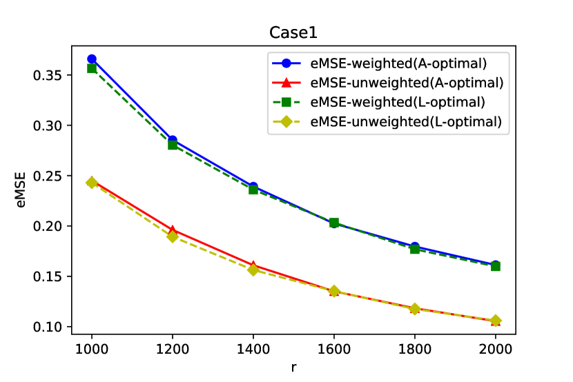
(a) Case1

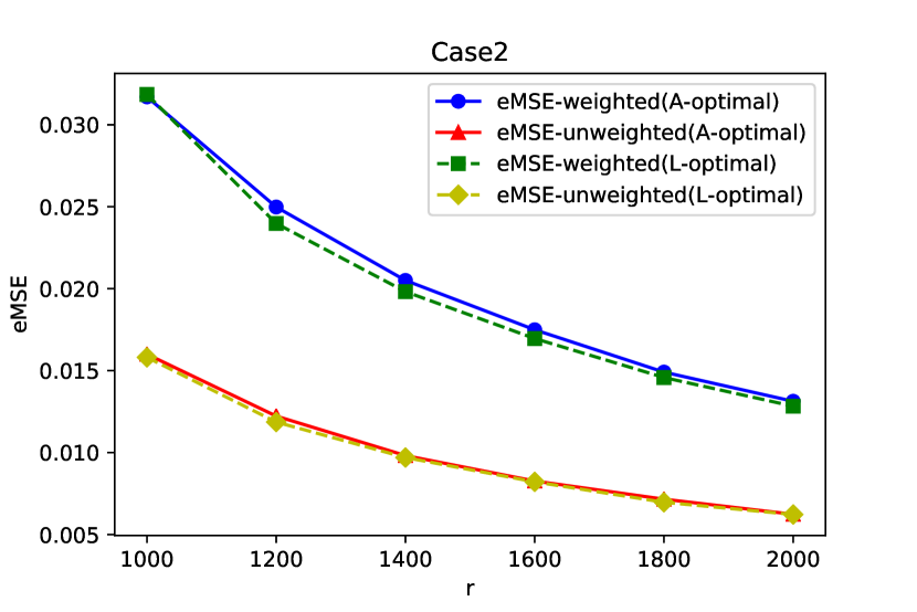
(b) Case2

Figure 3: eMSE for different subsample sizes $r$ with a pilot sample size $r_{\mathrm{p}}=500$ for Poisson regression under different settings.

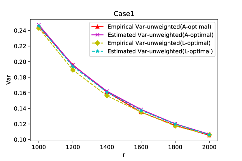
(a) Case1

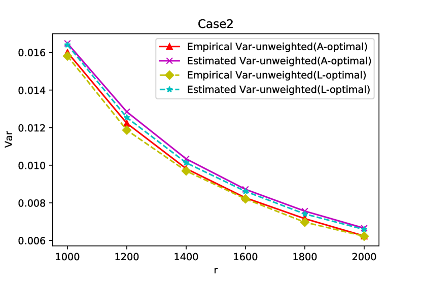
(b) Case2

Figure 4: Empirical variance and estimated variance, $\text{tr}\{\hat{\mathbb{V}}(\hat{\beta}_{\mathrm{uw}})\}$, for different subsample sizes $r$ with a pilot sample size $r_{\mathrm{p}}=500$ for the unweighted estimator under different settings.

4.1.2 Linear Model

We now present simulation results for linear regression. We used the settings in Zhang et al. (2021) which generated full data of size $n=100,000$ from the following model:

$$Y=X\beta_{0}+\epsilon,$$

where $\beta_{0}=(\underbrace{0.1,...,0.1}_{\text{5}},\underbrace{10,...,10}_{\text{20}},\underbrace{0.1,...,0.1}_{\text{5}})^{T}$ is a 30 dimensional vector, and $\epsilon\sim N(0,9I_{n})$. We used the following distributions of $X$:

1. GA: The covariate $X$ follows a multivariate normal distribution $N(1_{p},\Sigma_{2})$, where $p=30$, $\Sigma_{2}=U_{2}\Sigma U_{2}$ and $U_{2}=diag(5,5/2,...,5/30)$. The entries of $\Sigma$ are $\Sigma_{ij}=0.5^{I(i\neq j)}$, which is the same as we defined before.

2. T3: The covariate $X$ follows a multivariate t-distribution which has degrees of freedom 3, $T_{3}(0,\Sigma_{2})$, and $\Sigma_{2}$ is defined in GA above.

3. T1: The covariate $X$ follows a multivariate t-distribution which has degrees of freedom 1, $T_{1}(0,\Sigma_{2})$, and $\Sigma_{2}$ is the same as GA.

4. EXP: Components of $X$ are i.i.d. from an exponential distribution with a rate parameter of 2.

The first three settings are exactly the same settings used in Zhang et al. (2021). The last setting is used in Wang et al. (2019) and Wang (2019). Since the sampling probabilities are not related to the responses for linear models, Algorithm 1 can be simplified. For completeness, we present the simplified algorithm as Algorithm 2, which is similar to the algorithm used in Ma et al. (2015).

Algorithm 2 Unweighted estimation for linear model under measurement constraints

1:  Caculate the sampling probabilities $\{\pi_{i}\}_{i=1}^{n}$ using the following formula:

$$\pi_{i}^{\mathrm{A-OS}}=\frac{\left\|\left(\sum_{j=1}^{n}X_{j}X_{j}^{T}\right)^{-1}X_{i}\right\|}{\sum_{k=1}^{n}\left\|\left(\sum_{j=1}^{n}X_{j}X_{j}^{T}\right)^{-1}X_{k}\right\|}$$

2:  Obtain a subsample $\{(X_{i}^{*},Y_{i}^{*})\}_{i=1}^{r}$ of size $r$ according to the sampling probabilities $\{\pi_{i}^{\mathrm{A-OS}}\}_{i=1}^{n}$ using sampling with replacement, and solve the estimation equation

$$\Psi_{\mathrm{uw}}^{*}(\beta):=\frac{1}{r}\sum_{i=1}^{r}(X_{i}^{*{T}}\beta-Y_{i}^{*})X_{i}^{*}=0,$$

to obtain the unweighted estimator.

We also repeated the simulation for $S=500$ times and compared the empirical MSEs. In this section, we present the numerical results under A-optimality only. The results under L-optimality are similar and we present them in the supplementary material. Simulation results of unconditionally empirical MSE are presented in Figure 5. We see that the unweighted estimator is more efficient in every case. Especially, when $X$ has a $T_{3}$ or $T_{1}$ distribution, the unweighted estimator performs significantly better than the weighted estimator. As described in Zhang et al. (2021), the OSUMC estimator outperforms other sampling methods more obviously when $X$ is heavy-tailed. We notice that using the unweighted estimator, the advantage of OSUMC can be significantly reinforced when the design is heavy-tailed, despite $X$ not meeting the regularity conditions we presented in Section 3.

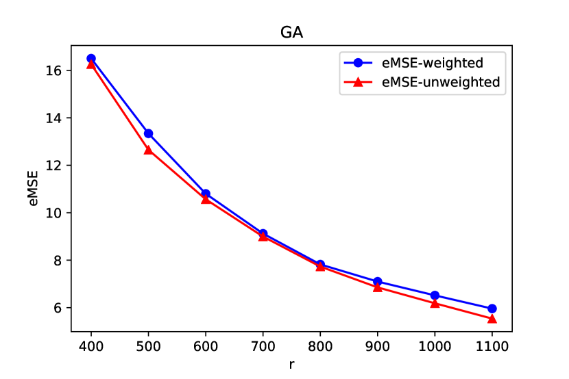
(a) GA

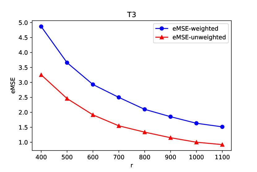
(b) T3

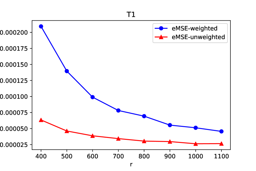
(c) T1

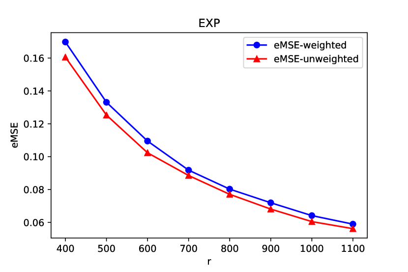
(d) EXP

Figure 5: eMSE for different subsample sizes $r$ for linear regression under different settings.

4.1.3 Computational Complexity

We present the computation times for the simulations based on logistic regression in Table 1. We used the same four settings for the logistic regression in Section 4.1.1, and repeated the experiments for $S=500$ times. We recorded the computing time for the weighted and unweighted procedures and implemented both $\pi^{\mathrm{A-OS}}$ and $\pi^{\mathrm{L-OS}}$ using Python. Our computations were carried out on a laptop running Windows 10 with an Intel i5 processor and 8GB memory, and we used the package: sklearn.linear_model.LogisticRegression for optimization. We present the results with subsample size $r=1000$. The results for other subsample size are similar and thus are omitted.

Table 1: Computational time (seconds)

	A-optimiality			L-optimality		Full data
	weighted	unweighted		weighted	unweighted
mzNormal	42.38	36.70		32.15	26.42	177.10
nzNormal	39.98	36.38		30.31	26.89	165.15
unNormal	41.20	37.47		32.61	28.69	256.45
mixNormal	40.97	36.14		31.92	27.45	162.44

In Table 1, both the weighted and unweighted subsample estimators significantly reduce the computation time compared with the MLE. The computation time of the unweighted estimator is not significantly different from that of the weighted estimator. The probabilities based on L-optimality reduce computation time more than the probabilities based on the A-optimality, in agreement with the analysis in Section 3. Interestingly, we see that the unweighted estimator is faster than the weighted estimator. This is because the target function of the unweighted estimator is usually smoother than that of the weighted estimator, and thus it takes fewer iterations for the algorithm to converge. To confirm this, we present the average numbers of iterations for optimizing the weighted and unweighted target functions in Table 2.

Table 2: Average number of iterations of the optimization algorithm

	A-optimiality			L-optimality
	weighted	unweighted		weighted	unweighted
mzNormal	18.53	10.68		18.51	10.77
nzNormal	19.08	10.85		18.74	10.88
unNormal	22.71	11.81		22.77	12.42
mixNormal	19.04	10.85		18.88	10.82

4.2 Experiments for real data

We apply our more efficient unweighted estimator to real data and evaluate its performance in this section.

4.2.1 Superconductivty Data Set

In this section, we apply our more efficient estimator to the superconductivty data set used in Zhang et al. (2021). The data set is available from the Machine Learning Repository at https://archive.ics.uci.edu/ml/datasets/Superconductivty+Data#. It contains 21,263 different data points, and every data point has 81 features with one continuous response. Each data point represents a superconductor. The response is the superconductor’s critical temperature and the features are extracted from its chemical formula. For example, the 81st column is the number of elements of the superconductor. We use standardized features as covariate variables and adopted a multiple linear regression model to fit the critical temperature from the chemical formula of the superconductor. Specially, the linear regression model is

$$Y=\beta^{(0)}+\beta^{(1)}Z_{1}+\beta^{(2)}Z_{2}+...+\beta^{(81)}Z_{81}+\epsilon,$$

where $Z_{i}$s represent the standardized features, $Y$ is the critical temperature, and $\epsilon$ is the normally distributed error. To measure the performances of sampling methods in parameter estimation, we use the empirical MSE of the estimator

$$\text{eMSE}(\hat{\beta})=\frac{1}{S}\sum_{s=1}^{S}\|\hat{\beta}^{(s)}-\hat{\beta}_{\text{MLE}}\|,$$ (14)

and the relative efficiency

$$\text{Relative Efficiency}=\frac{\text{eMSE}(\hat{\beta}_{\mathrm{w}})}{\text{eMSE}(\hat{\beta}_{\mathrm{uw}})},$$ (15)

where $\hat{\beta}^{(s)}$ represents the estimate in the $s$-th repetition. Here we use the full data estimator $\hat{\beta}_{\text{MLE}}$ instead of the “true” parameter $\beta_{0}$ to calculate eMSE because the true parameter is unknown for real data sets. We repeated the experiment for $S=1000$ times, and present the numerical results in Figure 6. Our unweighted estimator also outperforms the weighted estimator when applied to the Superconductivity data set and $\pi_{i}^{\mathrm{A-OS}}$ result in smaller eMSE than $\pi_{i}^{\mathrm{L-OS}}$ for both the weighted and unweighted estimators.

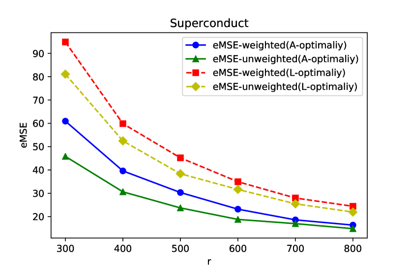
(a) eMSE

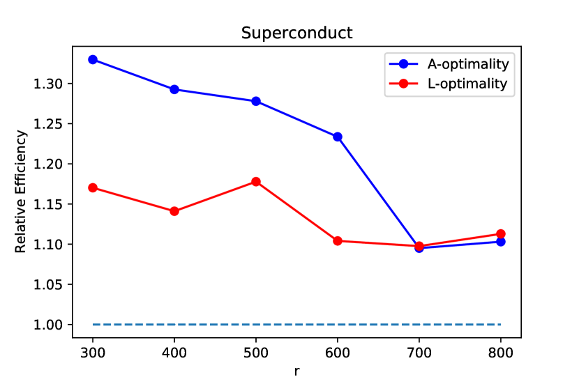
(b) Relative Efficiency

Figure 6: eMSE and Relative Efficiency for Superconductivty data set with different subsample data sizes $r$.

4.2.2 Supersymmetric Data Set

In this section, the supersymmetric (SUSY) benchmark data set is used to evaluate the performance of the unweighted estimator when applied to real data under logistic model. The SUSY data set is available from the Machine Learning Repository at https://archive.ics.uci.edu/ml/datasets/SUSY, and was also used in Wang et al. (2018) and Wang (2019). The data are composed of $n=5,000,000$ data points. Each data point represents a process and has one binary response with 18 covariates. The response variable represents whether the process produces new supersymmetric particles or the process is a background process. The kinematic features of the process are used as covariates. We used a logistic regression model to fit the data. Specifically, we model the probability that a process produces new supersymmetric particles as

$$P(Y=1|Z,\beta)=\frac{e^{\beta^{(0)}+\sum_{i=1}^{18}\beta^{(i)}Z_{i}}}{1+e^{\beta^{(0)}+\sum_{i=1}^{18}\beta^{(i)}Z_{i}}},$$

where $Z_{i}$’s are the kinematic features of a process. In order to compare the efficiency of parameter estimation, we again use the regression coefficient $\hat{\beta}_{\text{MLE}}$ derived from the full data as the “true parameter”. The empirical MSE of the estimator defined in (14) and the relative efficiency defined in (15) are also considered. We repeated the experiment for $S=1000$ times and drew a pilot subsample of size $r_{\mathrm{p}}=500$ in each repetition. Figure 7 shows that the unweighted estimator is over 130% more efficient than the weighted one when applied to the SUSY data set when using $\pi_{i}^{\mathrm{A-OS}}$, and over 110% more efficient when using $\pi^{\mathrm{L-OS}}$. Also, $\pi_{i}^{\mathrm{A-OS}}$ performs better than $\pi_{i}^{\mathrm{L-OS}}$ for the SUSY data set.

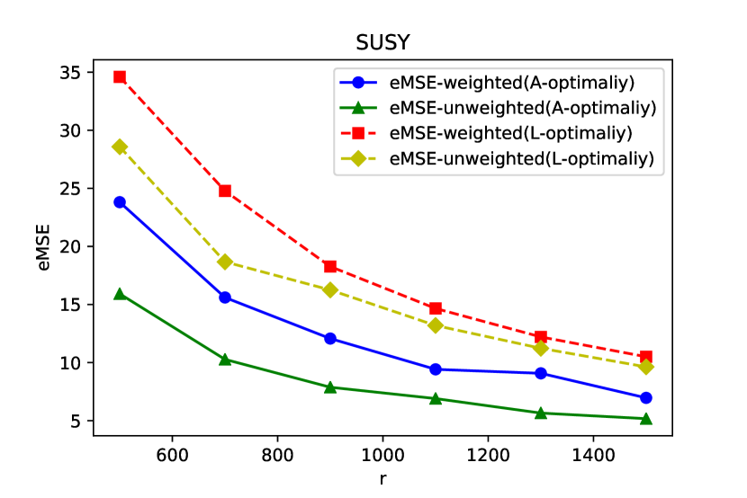
(a) eMSE

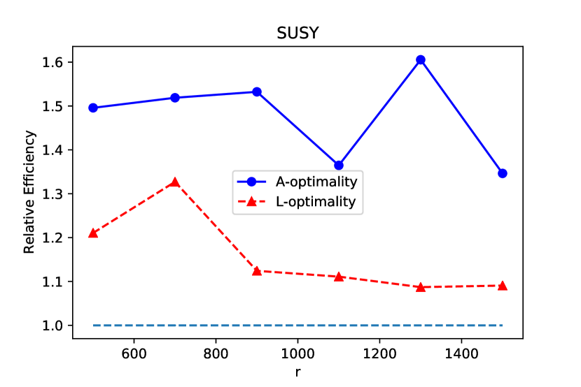
(b) Relative Efficiency

Figure 7: eMSE and Relative Efficiency for SUSY data set with different subsample data sizes $r$ and a pilot sample size $r_{\mathrm{p}}=500$.

5 CONCLUSION

We proposed a novel unweighted estimator based on OSUMC subsample for GLMs. It can be used to reduce computational burdens when responses are hard to acquire. A two-step scheme was proposed and we showed the asymptotic normality of the estimator unconditionally. We proved asymptotic results under a martingale framework without conditioning on pilot estimates. Furthermore, we showed that our new estimator is more efficient than the original OSUMC estimator for parameter estimation under subsampling settings. Several numerical experiments were implemented to demonstrate the superiouity of our unweighted estimator over the original weighted esitmator.

Some extensions may be interesting for future research. Sampling with replacement is used for both the weighted estimator and our new unweighted estimator based on OSUMC. Poisson sampling is an alternative that reduces the RAM usage for subsampling methods. Therefore, Poisson sampling is worth developing under measurement constraints. Extending our subsampling procedure to models beyond GLMs is also an interesting topic for future studies.

Appendix A Proofs and technical details

In this appendix, we provide proofs in Section 3. Technical details related to asymptotic results are presented in Section A.1; technical details related to estimation efficiency are presented in Section A.2.

A.1 Proofs of asymptotic results

We present proofs of the asymptotic results in this section. The proof of Lemma 1 is presented in Section A.1.1. The proof of Lemma 2 is presented in Section A.1.3. The proof of Theorem 1 is presented in Section A.1.3. We first recall some notations defined in the main paper:

$$\Psi_{\mathrm{uw}}^{*}(\beta)=\frac{1}{r}\sum_{i=1}^{r}\{b^{{}^{\prime}}(X_{i}^{*{T}}\beta)-Y_{i}^{*}\}X_{i}^{*},$$

$$\hat{m}=\frac{1}{n}\sum_{i=1}^{n}\sqrt{b^{{}^{\prime\prime}}(X_{i}^{T}\hat{\beta}_{\mathrm{p}})}\|L\hat{\Phi}_{\mathrm{p}}^{-1}X_{i}\|,$$

$$\Phi=\mathbb{E}\left\{\frac{1}{n}\sum_{i=1}^{n}b^{{}^{\prime\prime}}(X_{i}^{T}\beta_{0})X_{i}X_{i}^{T}\right\}=\mathbb{E}\{b^{{}^{\prime\prime}}(X^{T}\beta_{0})XX^{T}\},$$

and

$$\hat{\Phi}_{\mathrm{p}}=\frac{1}{r_{\mathrm{p}}}\sum_{i=1}^{r_{\mathrm{p}}}b^{{}^{\prime\prime}}(X_{i}^{*_{\mathrm{p}}{T}}\hat{\beta}_{\mathrm{p}})X_{i}^{*_{\mathrm{p}}}X_{i}^{*_{\mathrm{p}}{T}}.$$

In the following, we denote

$$\Psi_{\mathrm{uw}}^{*\mathrm{m}}:=\hat{m}\Psi_{\mathrm{uw}}^{*}(\beta)=\hat{m}\frac{1}{r}\sum_{i=1}^{r}\{b^{{}^{\prime}}(X_{i}^{*{T}}\beta)-Y_{i}^{*}\}X_{i}^{*}.$$

Here we use $\hat{m}$ to rescale the score function in order to simplify the proof. We also denote

$$M_{n,i}:=\hat{m}\{b^{{}^{\prime}}(X_{i}^{*{T}}\beta)-Y_{i}^{*}\}X_{i}^{*}-Q,$$

and

$$Q:=\frac{1}{n}\sum_{j=1}^{n}\sqrt{b^{{}^{\prime\prime}}(X_{j}^{T}\hat{\beta}_{\mathrm{p}})}\|L\hat{\Phi}_{\mathrm{p}}^{-1}X_{j}\|\{b^{{}^{\prime}}(X_{j}^{T}\beta)-Y_{j}\}X_{j}.$$

We then have

$$\Psi^{*\mathrm{m}}_{\mathrm{uw}}(\beta)=\frac{1}{r}\sum_{i=1}^{r}M_{n,i}+Q.$$

For filtration $\{\mathcal{F}_{n,i}\}_{i=1}^{r}$: $\mathcal{F}_{n,0}=\sigma(X_{1}^{n},Y_{1}^{n},\hat{\beta}_{\mathrm{p}},\hat{\Phi}_{\mathrm{p}})$; $\mathcal{F}_{n,1}=\sigma(X_{1}^{n},Y_{1}^{n},\hat{\beta}_{p},\hat{\Phi}_{\mathrm{p}})\lor\sigma(*_{1})$;$\dots$;$\mathcal{F}_{n,i}=\sigma(X_{1}^{n},Y_{1}^{n},\hat{\beta}_{\mathrm{p}},\hat{\Phi}_{\mathrm{p}})\lor\sigma(*_{1})\lor\dots\lor\sigma(*_{i})$, where $\sigma(*_{i})$ is the $\sigma$-algebra generated by the $i$-th sampling step, we have

$$\mathbb{E}(M_{n,i}|\mathcal{F}_{n,i-1}) =\mathbb{E}\left[\hat{m}\{b^{{}^{\prime}}(X_{i}^{*{T}}\beta)-Y_{i}^{*}\}X_{i}^{*}|\mathcal{F}_{n,i-1}\right]-Q$$

$$=\hat{m}\sum_{j=1}^{n}\pi_{j}^{\mathrm{OS}}(\hat{\beta}_{\mathrm{p}},\hat{\Phi}_{\mathrm{p}})\{b^{{}^{\prime}}(X_{j}^{T}\beta)-Y_{j}\}X_{j}-Q.$$

Since

$$\pi_{j}^{\mathrm{OS}}(\hat{\beta}_{\mathrm{p}},\hat{\Phi}_{\mathrm{p}})=\frac{\sqrt{b^{{}^{\prime\prime}}(X_{j}^{T}\hat{\beta}_{\mathrm{p}})}\|L\hat{\Phi}_{\mathrm{p}}^{-1}X_{j}\|}{\sum_{i=1}^{n}\sqrt{b^{{}^{\prime\prime}}(X_{i}^{T}\hat{\beta}_{\mathrm{p}})}\|L\hat{\Phi}_{\mathrm{p}}^{-1}X_{i}\|}=\frac{\sqrt{b^{{}^{\prime\prime}}(X_{j}^{T}\hat{\beta}_{\mathrm{p}})}\|L\hat{\Phi}_{\mathrm{p}}^{-1}X_{j}\|}{n\hat{m}},$$

we obtain that

$$\mathbb{E}(M_{n,i}|\mathcal{F}_{n,i-1})=0.$$

Therefore, $M_{n,i}$ is a martingale difference sequence, and we now present some lemmas we will use to prove asymptotic results.

Lemma A.3 (Martingale Law of Large Numbers).

If triangle array $(M_{n,i})_{i=1}^{r}$ is a martingale difference sequence, and uniformly integrable:

$$\lim_{B\to\infty}\sup_{n,i}\mathbb{E}\left[\|M_{n,i}\|I\{\|M_{n,i}\|\geq B\}\right]=0,$$

then

$$\mathbb{E}\left\{\left|\frac{1}{r}\sum_{i=1}^{r}M_{n,i}\right|\right\}\to 0.$$

Remark 3.

This is a direct corollary of Theorem 2(b) in Andrews (1988), which is mentioned in Section 3 of Andrews (1988). Specially, if $(M_{n,i})_{i=1}^{r}$ is an identically distributed martingale difference sequence for fixed $n$, which is the case for sampling with replacement, we only need that $(M_{n,i})_{i=1}^{r}$ is uniformly integrable for index $n$, since

$$\sup_{n}\mathbb{E}\left[\|M_{n,1}\|I\{\|M_{n,1}\|\geq B\}\right]=\sup_{n,i}\mathbb{E}\left[\|M_{n,i}\|I\{\|M_{n,i}\|\geq B\}\right].$$

Lemma A.4.

Let $\mathbf{v_{1}}$,…,$\mathbf{v_{n}}$ be i.i.d random vector with the same distribution of $\mathbf{v}$. Let $g_{1}$ be a bounded function that may depend on $n$ and other random variables, and $g_{2}$ be a fixed function that does not depend on $n$. If $g_{1}(\mathbf{v_{i}})=o_{p}(1)$ for each $i$ as $n\to\infty$, and $\mathbb{E}|g_{2}(\mathbf{v})|<\infty$, then

$$\frac{1}{n}\sum_{i=1}^{n}g_{1}(\mathbf{v_{i}})g_{2}(\mathbf{v_{i}})=o_{p}(1).$$

This is Lemma 1 in Wang (2019).

Lemma A.5.

Let $M$, $N$ be self-adjoint $k\times k$ matrices, and $m_{j}$, $n_{j}$ be their eigenvalues arranged in increasing order. Then

$$\sum(n_{j}-m_{j})^{2}\leq\|N-M\|_{F}^{2}.$$

This lemma is usually referred to as the Hoffman-Wielandt inequality, see Theorem 18 in Chapter 10 of Lax (2007). Before we prove the main results, we first prove Lemma A.6.

Lemma A.6.

There exists an $r_{*}$ such that when $r_{\mathrm{p}}\geq r_{*}$ , $\lambda_{\max}(\hat{\Phi}_{\mathrm{p}}^{-1})<C$ a.s., where $C$ is a finite constant. In addition, we have $\hat{\beta}_{\mathrm{p}}\xrightarrow{p}\beta_{0}$ and $\hat{\Phi}_{\mathrm{p}}\xrightarrow{p}\Phi$, as $r_{\mathrm{p}}\to\infty$.

Proof.

We have

$$\hat{\Phi}_{\mathrm{p}}=\frac{1}{r_{\mathrm{p}}}\sum_{i=1}^{r_{\mathrm{p}}}b^{{}^{\prime\prime}}(X_{i}^{*_{\mathrm{p}}}\hat{\beta}_{\mathrm{p}})X_{i}^{*_{\mathrm{p}}}X_{i}^{*_{\mathrm{p}}{T}}\geq\frac{1}{r_{\mathrm{p}}}\sum_{i=1}^{r_{\mathrm{p}}}g(X_{i}^{*_{\mathrm{p}}})X_{i}^{*_{\mathrm{p}}}X_{i}^{*_{\mathrm{p}}{T}},$$

and therefore

$$\hat{\Phi}_{\mathrm{p}}^{-1}\leq\left\{\frac{1}{r_{\mathrm{p}}}\sum_{i=1}^{r_{\mathrm{p}}}g(X_{i}^{*_{\mathrm{p}}})X_{i}^{*_{\mathrm{p}}}X_{i}^{*_{\mathrm{p}}{T}}\right\}^{-1}.$$

Then, we have

$$\lambda_{\max}\left(\hat{\Phi}_{\mathrm{p}}^{-1}\right)\leq\lambda_{\max}\left[\left\{\frac{1}{r_{\mathrm{p}}}\sum_{i=1}^{r_{\mathrm{p}}}g(X_{i}^{*_{\mathrm{p}}})X_{i}^{*_{\mathrm{p}}}X_{i}^{*_{\mathrm{p}}{T}}\right\}^{-1}\right]$$

$$\leq\lambda_{\max}\left[\mathbb{E}\{g(X)XX^{T}\}^{-1}\right]+\left|\lambda_{\max}\left[\left\{\frac{1}{r_{\mathrm{p}}}\sum_{i=1}^{r_{\mathrm{p}}}g(X_{i}^{*_{\mathrm{p}}})X_{i}^{*_{\mathrm{p}}}X_{i}^{{}^{*_{\mathrm{p}}{T}}}\right\}^{-1}\right]-\lambda_{\max}\left[\mathbb{E}\{g(X)XX^{T}\}^{-1}\right]\right|$$

$$\leq\lambda_{\max}\left[\mathbb{E}\{g(X)XX^{T}\}^{-1}\right]+\left\|\left\{\frac{1}{r_{\mathrm{p}}}\sum_{i=1}^{r_{\mathrm{p}}}g(X_{i}^{*_{\mathrm{p}}})X_{i}^{*_{\mathrm{p}}}X_{i}^{*_{0}^{T}}\right\}^{-1}-\mathbb{E}\{g(X)XX^{T}\}^{-1}\right\|_{F},$$

the last inequality is due to Lemma A.5. Applying the Strong Law of Large Numbers, we obtain

$$\left\|\left\{\frac{1}{r_{\mathrm{p}}}\sum_{i=1}^{r_{\mathrm{p}}}g(X_{i}^{*_{\mathrm{p}}})X_{i}^{*_{\mathrm{p}}}X_{i}^{*_{\mathrm{p}}{T}}\right\}^{-1}-\mathbb{E}\{g(X)XX^{T}\}^{-1}\right\|_{F}=o(1),$$

and therefore we can find a constant $C$ and a $r_{*}$ such that

$$\lambda_{\max}\left(\hat{\Phi}_{\mathrm{p}}^{-1}\right)<C,$$

when $r>r_{*}$.

Next, we prove the second part of the lemma. Since we use simple random sampling in Algorithm 1, the asymptotic property of $\hat{\beta}_{\mathrm{p}}$ is the same as i.i.d data. Thus, the consistency of $\hat{\beta}_{\mathrm{p}}$ is easy to obtain, see McCullagh & Nelder (1989). Now, we know that $b^{{}^{\prime\prime}}(X_{i}^{*_{\mathrm{p}}{T}}\hat{\beta}_{\mathrm{p}})-b^{{}^{\prime\prime}}(X_{i}^{*_{\mathrm{p}}{T}}\beta_{0})$ is $o_{p}(1)$ and bounded and

$$\left\|\mathbb{E}\left(X_{i}^{*_{\mathrm{p}}}X_{i}^{*_{\mathrm{p}}{T}}\right)\right\|_{F}\leq\mathbb{E}(\|X_{i}^{*_{\mathrm{p}}}\|^{2})<\infty.$$

By Lemma A.4 and the Law of Large Numbers, we have

$$\hat{\Phi}_{\mathrm{p}}\xrightarrow{p}\Phi.$$

This complete the proof. ∎

Therefore, in the rest of the paper, we always assume that

$$\lambda_{\max}(\hat{\Phi}_{\mathrm{p}}^{-1})\leq C.$$

Now, we show the proofs of asymptotic results presented in Section 3.

A.1.1 Proof of Lemma 1

We prove Lemma 1 in this section, and we first introduce some notations we use in this section. We have already defined

$$\Gamma(\beta)=\mathbb{E}\left\{\sqrt{b^{{}^{\prime\prime}}(X^{T}\beta_{0})}\|L\Phi^{-1}X\|b^{{}^{\prime\prime}}(X^{T}\beta)XX^{T}\right\}.$$

Denote

$$\tilde{M}_{n,i}=\hat{m}b^{{}^{\prime\prime}}(X_{i}^{*{T}}\beta)X_{i}^{*}X_{i}^{*{T}}-\tilde{Q},$$

$$\tilde{Q}=\frac{1}{n}\sum_{j=1}^{n}\sqrt{b^{{}^{\prime\prime}}(X_{j}^{T}\hat{\beta}_{\mathrm{p}})}\|L\hat{\Phi}_{\mathrm{p}}^{-1}X_{j}\|b^{{}^{\prime\prime}}(X_{j}^{T}\beta)X_{j}X_{j}^{T}.$$

Then, we have

$$\dot{\Psi}_{\mathrm{uw}}^{*\mathrm{m}}(\beta)-\Gamma(\beta)=\frac{1}{r}\sum_{i=1}^{r}\tilde{M}_{n,i}+\tilde{Q}-\Gamma(\beta).$$

For filtration $\{\mathcal{F}_{n,i}\}_{i=1}^{r}$: $\mathcal{F}_{n,0}=\sigma(X_{1}^{n},Y_{1}^{n},\hat{\beta}_{\mathrm{p}},\hat{\Phi}_{\mathrm{p}})$; $\mathcal{F}_{n,1}=\sigma(X_{1}^{n},Y_{1}^{n},\hat{\beta}_{\mathrm{p}},\hat{\Phi}_{\mathrm{p}})\lor\sigma(*_{1})$; $\dots$;$\mathcal{F}_{n,i}=\sigma(X_{1}^{n},Y_{1}^{n},\hat{\beta}_{\mathrm{p}},\hat{\Phi}_{\mathrm{p}})\lor\sigma(*_{1})\lor\dots\lor\sigma(*_{i})$, we have

$$\mathbb{E}(\tilde{M}_{n,i}|\mathcal{F}_{n,i-1})=0.$$

Therefore, $\tilde{M}_{n,i}$ is a martingale difference sequence. If we denote

$$\hat{w}_{i}=\sqrt{b^{{}^{\prime\prime}}(X_{i}^{T}\hat{\beta}_{\mathrm{p}})}\|L\hat{\Phi}_{\mathrm{p}}^{-1}X_{i}\|>0,$$

we will then know that

$$\hat{m}=\frac{1}{n}\sum_{j=1}^{n}\hat{w}_{j},$$

and

$$|\hat{w}_{i}|\lesssim\|L\hat{\Phi}_{\mathrm{p}}^{-1}X_{i}\|\lesssim\|X_{i}\|,$$

due to Assumption 1 and Lemma A.6, where the notion “$\lesssim$” means that there exist a constant $K$, such that $\hat{w}_{i}\leq K\|X_{i}\|$. Now, we present the proof of Lemma 1.

Proof of Lemma 1.

To show that $\dot{\Psi}_{\mathrm{uw}}^{*\mathrm{m}}(\beta_{n})\xrightarrow{p}\Gamma$ for every sequence $\beta_{n}\xrightarrow{p}\beta_{0}$, we first show that for every $\beta\in\mathbb{B}$,

$$\dot{\Psi}_{\mathrm{uw}}^{*\mathrm{m}}(\beta)-\Gamma(\beta)=\hat{m}\frac{1}{r}\sum_{i=1}^{r}b^{{}^{\prime\prime}}(X_{i}^{*{T}}\beta)X_{i}^{*}X_{i}^{*{T}}-\Gamma(\beta)=o_{p}(1),$$

where

$$\Gamma(\beta):=\mathbb{E}\left\{\sqrt{b^{{}^{\prime\prime}}(X^{T}\beta_{0})}\|L\Phi^{-1}X\|b^{{}^{\prime\prime}}(X^{T}\beta)XX^{T}\right\}.$$

We already know that

$$\dot{\Psi}_{\mathrm{uw}}^{*\mathrm{m}}(\beta)-\Gamma(\beta)=\frac{1}{r}\sum_{i=1}^{r}\tilde{M}_{n,i}+\tilde{Q}-\Gamma(\beta),$$

and $(\tilde{M}_{n,i})_{i}^{r}$ is an identically distributed martingale difference sequence. Therefore, for each entry of $\dot{\Psi}_{\mathrm{uw}}^{*\mathrm{m}}(\beta)$, assuming $0<\delta<1$, we have

$$\left\{\mathbb{E}\left(\left|\tilde{M}_{n,1}^{(lk)}\right|^{1+\delta}\right)\right\}^{\frac{1}{1+\delta}}$$

$$\leq\left[\mathbb{E}\left\{\left|\hat{m}b^{{}^{\prime\prime}}(X_{1}^{*{T}}\beta)X_{1}^{*{(l)}}X_{1}^{*{(k)}}\right|^{1+\delta}\right\}\right]^{\frac{1}{1+\delta}}+\left[\mathbb{E}\left\{\left|\frac{1}{n}\sum_{j=1}^{n}\hat{w}_{j}b^{{}^{\prime\prime}}(X_{j}^{T}\beta)X_{j}^{(l)}X_{j}^{(k)}\right|^{1+\delta}\right\}\right]^{\frac{1}{1+\delta}}$$

$$:=I_{1}^{\frac{1}{1+\delta}}+I_{2}^{\frac{1}{1+\delta}},$$

due to the Minkowski inequality. Then, for $I_{1}$, we have

$$I_{1} \lesssim\mathbb{E}\left(\hat{m}^{1+\delta}\left|X_{1}^{*{(l)}}X_{1}^{*{(k)}}\right|^{1+\delta}\right)=\mathbb{E}\left\{\mathbb{E}\left(\hat{m}^{1+\delta}\left|X_{1}^{*{(l)}}X_{1}^{*{(k)}}\right|^{1+\delta}\bigg{|}\mathcal{F}_{n,0}\right)\right\}$$

$$=\mathbb{E}\left(\hat{m}^{\delta}\frac{1}{n}\sum_{j=1}^{n}\hat{w}_{j}\left|X_{j}^{(l)}X_{j}^{(k)}\right|^{1+\delta}\right)\lesssim\mathbb{E}\left\{\left(\frac{1}{n}\sum_{i=1}^{n}\|X_{i}\|\right)^{\delta}\frac{1}{n}\sum_{j=1}^{n}\|X_{j}\|\left|X_{j}^{(l)}X_{j}^{(k)}\right|^{1+\delta}\right\}$$

$$\leq\left\{\mathbb{E}\left(\frac{1}{n}\sum_{i=1}^{n}\|X_{i}\|\right)\right\}^{\delta}\left[\mathbb{E}\left\{\left(\frac{1}{n}\sum_{j=1}^{n}\|X_{j}\|\left|X_{j}^{(l)}X_{j}^{(k)}\right|^{1+\delta}\right)^{\frac{1}{1-\delta}}\right\}\right]^{1-\delta}.$$

The last inequality is due to the Hölder inequality when $p=1/\delta$ and $q=1/(1-\delta)$. Since $1/(1-\delta)>1$, we then use the Minkowski inequality and obtain

$$I_{1} \lesssim\left\{\mathbb{E}\left(\frac{1}{n}\sum_{i=1}^{n}\|X_{i}\|\right)\right\}^{\delta}\left[\frac{1}{n}\sum_{j=1}^{n}\mathbb{E}\left\{\left(\|X_{j}\|\left|X_{j}^{(l)}X_{j}^{(k)}\right|^{1+\delta}\right)^{\frac{1}{1-\delta}}\right\}\right]^{1-\delta}$$

$$\leq\left\{\mathbb{E}\left(\|X\|\right)\right\}^{\delta}\left\{\mathbb{E}\left(\|X\|^{\frac{1}{1-\delta}}\left|X^{(l)}X^{(k)}\right|^{\frac{1+\delta}{1-\delta}}\right)\right\}^{1-\delta}.$$

For $I_{2}$, applying the Minkowski inequality, we obtain

$$I_{2} \leq\frac{1}{n}\sum_{j=1}^{n}\mathbb{E}\left\{\left|\hat{w}_{j}b^{{}^{\prime\prime}}(X_{j}^{T}\beta)X_{j}^{(l)}X_{j}^{(k)}\right|^{1+\delta}\right\}$$

$$\lesssim\mathbb{E}\left(\|X\|^{1+\delta}|X^{(l)}X^{(k)}|^{1+\delta}\right).$$

To see $\mathbb{E}\left(\|X\|^{\frac{1}{1-\delta}}\left|X^{(l)}X^{(k)}\right|^{\frac{1+\delta}{1-\delta}}\right)<\infty$, we only need to add all the entries:

$$\sum_{l,k}\mathbb{E}\left(\|X\|^{\frac{1}{1-\delta}}\left|X^{(l)}X^{(k)}\right|^{\frac{1+\delta}{1-\delta}}\right)=\sum_{l,k}\mathbb{E}\left(\|X\|^{\frac{1}{1-\delta}}\left|X^{(l)}\right|^{\frac{1+\delta}{1-\delta}}\left|X^{(k)}\right|^{\frac{1+\delta}{1-\delta}}\right)\lesssim\mathbb{E}\left(\|X\|^{\frac{3+2\delta}{1-\delta}}\right),$$

Similarly, we also have

$$\sum_{l,k}\mathbb{E}\left(\|X\|^{1+\delta}|X^{(l)}X^{(k)}|^{1+\delta}\right)\lesssim\mathbb{E}\left(\|X\|^{3+3\delta}\right).$$

If we let $\delta=1/6$, we then have

$$\mathbb{E}\left(\|X\|^{\frac{3+2\delta}{1-\delta}}\right)=\mathbb{E}(\|X\|^{4})<\infty,$$

and

$$\mathbb{E}\left(\|X\|^{3+3\delta}\right)=\mathbb{E}\left(\|X\|^{3.5}\right)<\infty.$$

Therefore, $\sup_{n}\mathbb{E}(|\tilde{M}_{n,1}^{(lk)}|^{1+\delta})<\infty$ and we know that $(\tilde{M}_{n,i})_{i}^{r}$ is $L^{1}$ uniformly integrable. Now applying Lemma A.3, we can show that

$$\frac{1}{r}\sum_{i=1}^{r}\tilde{M}_{n,i}=o_{p}(1).$$

Next, we prove

$$\tilde{Q}-\Gamma(\beta)$$

$$=\frac{1}{n}\sum_{j=1}^{n}\hat{w}_{j}b^{{}^{\prime\prime}}(X_{j}^{T}\beta)X_{j}X{j}^{T}-\mathbb{E}\left\{\sqrt{b^{{}^{\prime\prime}}(X^{T}\beta_{0})}\|L\Phi^{-1}X\|b^{{}^{\prime\prime}}(X^{T}\beta)XX^{T}\right\}$$

$$=o_{p}(1).$$

For the consistency of $\hat{\beta}_{\mathrm{p}}$ and $\hat{\Phi}_{\mathrm{p}}^{-1}$, it is easy to know that

$$\sqrt{b^{{}^{\prime\prime}}(X_{j}^{T}\hat{\beta}_{\mathrm{p}})}\|L\hat{\Phi}_{\mathrm{p}}^{-1}X_{j}\|-\sqrt{b^{{}^{\prime\prime}}(X_{j}^{T}\beta_{0})}\|L\Phi^{-1}X_{j}\|=o_{p}(1).$$

Considering each entry of $\tilde{Q}$ and $\Gamma(\beta)$, we know that

$$\frac{1}{n}\sum_{j=1}^{n}\hat{w}_{j}b^{{}^{\prime\prime}}(X_{j}^{T}\beta)X_{j}^{(l)}X_{j}^{(k)}-\frac{1}{n}\sum_{j=1}^{n}\sqrt{b^{{}^{\prime\prime}}(X_{j}^{T}\beta_{0})}\|L\Phi^{-1}X_{j}\|b^{{}^{\prime\prime}}(X_{j}^{T}\beta)X_{j}^{(l)}X_{j}^{(k)}$$

$$=\frac{1}{n}\sum_{j=1}^{n}\left\{\sqrt{b^{{}^{\prime\prime}}(X_{j}^{T}\hat{\beta}_{\mathrm{p}})}\|L\hat{\Phi}_{\mathrm{p}}^{-1}X_{j}\|-\sqrt{b^{{}^{\prime\prime}}(X_{j}^{T}\beta_{0})}\|L\Phi^{-1}X_{j}\|\right\}b^{{}^{\prime\prime}}(X_{j}^{T}\beta)X_{j}^{(l)}X_{j}^{(k)}.$$

Then, since we include intercept in the model we know $\|X_{j}\|\geq 1$, and thus we have

$$\frac{1}{n}\sum_{j=1}^{n}\left\{\sqrt{b^{{}^{\prime\prime}}(X_{j}^{T}\hat{\beta}_{\mathrm{p}})}\|L\hat{\Phi}_{\mathrm{p}}^{-1}X_{j}\|-\sqrt{b^{{}^{\prime\prime}}(X_{j}^{T}\beta_{0})}\|L\Phi^{-1}X_{j}\|\right\}b^{{}^{\prime\prime}}(X_{j}^{T}\beta)X_{j}^{(l)}X_{j}^{(k)}$$

$$=\frac{1}{n}\sum_{j=1}^{n}\left\{\sqrt{b^{{}^{\prime\prime}}(X_{j}^{T}\hat{\beta}_{\mathrm{p}})}\frac{\|L\hat{\Phi}_{\mathrm{p}}^{-1}X_{j}\|}{\|X_{j}\|}-\sqrt{b^{{}^{\prime\prime}}(X_{j}^{T}\beta_{0})}\frac{\|L\Phi^{-1}X_{j}\|}{\|X_{j}\|}\right\}\|X_{j}\|b^{{}^{\prime\prime}}(X_{j}^{T}\beta)X_{j}^{(l)}X_{j}^{(k)}.$$

We know that

$$\frac{\|L\Phi^{-1}X_{j}\|}{\|X_{j}\|}\leq C,\quad and\quad\frac{\|L\hat{\Phi}_{\mathrm{p}}^{-1}X_{j}\|}{\|X_{j}\|}\leq C,$$

which means

$$\left\{\sqrt{b^{{}^{\prime\prime}}(X_{j}^{T}\hat{\beta}_{\mathrm{p}})}\frac{\|L\hat{\Phi}_{\mathrm{p}}^{-1}X_{j}\|}{\|X_{j}\|}-\sqrt{b^{{}^{\prime\prime}}(X_{j}^{T}\beta_{0})}\frac{\|L\Phi^{-1}X_{j}\|}{\|X_{j}\|}\right\}$$

is bounded and also is $o_{p}(1)$. We now show that $\|X_{j}\|b^{{}^{\prime\prime}}(X_{j}^{T}\beta)X_{j}^{(l)}X_{j}^{(k)}$ is integrable, since

$$\mathbb{E}\left\{\|X_{j}\|b^{{}^{\prime\prime}}(X_{j}^{T}\beta)|X^{(l)}|\cdot|X^{(k)}|\right\} \lesssim\mathbb{E}\left(\|X_{j}\|\cdot|X^{(l)}|\cdot|X^{(k)}|\right)$$

$$\leq\sum_{l,k}\mathbb{E}\left(\|X_{j}\|\cdot|X^{(l)}|\cdot|X^{(k)}|\right)$$

$$\lesssim\mathbb{E}\left(\|X_{j}\|^{3}\right)<\infty.$$

Then, applying Lemma A.4 and the Law of Large Numbers, we have

$$\tilde{Q}^{(lk)}-\Gamma(\beta)^{(lk)}$$

$$=\frac{1}{n}\sum_{j=1}^{n}\sqrt{b^{{}^{\prime\prime}}(X_{j}^{T}\beta_{0})}\|L\Phi^{-1}X_{j}\|b^{{}^{\prime\prime}}(X_{j}^{T}\beta)X_{j}^{(l)}X_{j}^{(k)}-\Gamma(\beta)^{(lk)}+o_{p}(1)$$

$$=o_{p}(1),$$

which means $\tilde{Q}-\Gamma(\beta)=o_{p}(1)$. Therefore,

$$\dot{\Psi}_{\mathrm{uw}}^{*\mathrm{m}}(\beta)-\Gamma(\beta)=o_{p}(1).$$

We have already proved that $\dot{\Psi}_{\mathrm{uw}}^{*\mathrm{m}}(\beta)\xrightarrow{p}\Gamma(\beta)$, for every $\beta\in\mathbb{B}$, and we next prove $\dot{\Psi}_{\mathrm{uw}}^{*\mathrm{m}}(\beta_{n})\xrightarrow{p}\Gamma$, for every sequence $\beta_{n}\xrightarrow{p}\beta_{0}$. For each entry of $\dot{\Psi}_{n}^{*}(\beta)$ and $\Gamma(\beta)$, taking $\beta_{1},\beta_{2}\in\mathbb{B}$, we use the mean value theorem and obtain

$$\left|\left\{\dot{\Psi}_{\mathrm{uw}}^{*\mathrm{m}}(\beta_{1})^{(lk)}-\Gamma(\beta_{1})^{(lk)}\right\}-\left\{\dot{\Psi}_{\mathrm{uw}}^{*\mathrm{m}}(\beta_{2})^{(lk)}-\Gamma(\beta_{2})^{(lk)}\right\}\right|$$

$$=\bigg{\|}\bigg{\{}\hat{m}\frac{1}{r}\sum_{i=1}^{r}b^{{}^{\prime\prime\prime}}(X_{i}^{*{T}}\tilde{\beta_{1}})X_{i}^{*{(l)}}X_{i}^{*{(k)}}X_{i}^{*}$$

$$\quad-\mathbb{E}[\sqrt{b^{{}^{\prime\prime}}(X^{T}\beta_{0})}\|L\Phi^{-1}X\|b^{{}^{\prime\prime\prime}}(X^{T}\tilde{\beta}_{2})X^{(l)}X^{(k)}X]\bigg{\}}\cdot(\beta_{1}-\beta_{2})\bigg{\|}$$

$$\lesssim\left\{\hat{m}\frac{1}{r}\sum_{i=1}^{r}h(X_{i}^{*})\left|X_{i}^{*{(l)}}X_{i}^{*{(k)}}\right|\|X_{i}^{*}\|+O(1)\right\}\|\beta_{1}-\beta_{2}\|$$

$$:=L_{n}\|\beta_{1}-\beta_{2}\|,$$

the second inequality is due to Assumption 3. Then, we need to show $L_{n}=O_{p}(1)$. Actually, we know that

$$\mathbb{E}\left\{\hat{m}\frac{1}{r}\sum_{i=1}^{r}h(X_{i}^{*})\left|X_{i}^{*{(l)}}X_{i}^{*{(k)}}\right|\|X_{i}^{*}\|\right\} =\mathbb{E}\left\{\frac{1}{n}\sum_{j=1}^{n}\hat{w}_{j}h(X_{j})\left|X_{j}^{(l)}X_{j}^{(k)}\right\rvert\|X_{j}\|\right\}$$

$$\lesssim\mathbb{E}\left\{\frac{1}{n}\sum_{j=1}^{n}h(X_{j})\left|X_{j}^{(l)}X_{j}^{(k)}\right\rvert\|X_{j}\|^{2}\right\}$$

$$=\mathbb{E}\left\{h(X)\left|X^{(l)}X^{(k)}\right|\|X\|^{2}\right\},$$

and $\mathbb{E}\left\{h(X)\left|X^{(l)}X^{(k)}\right\rvert\|X\|^{2}\right\}\leq\sum_{l,k}\mathbb{E}\left\{h(X)\left|X^{(l)}X^{(k)}\right|\|X\|^{2}\right\}\lesssim\mathbb{E}\left\{h(X)\|X\|^{4}\right\}<\infty$, which is guaranteed because of Assumption 3; therefore, $L_{n}$ is $O_{p}(1)$. Now we apply Theorem 21.10 in Davidson (1994) to conclude that $\dot{\Psi}_{\mathrm{uw}}^{*\mathrm{m}}(\beta)-\Gamma(\beta)$ is stochastic equicontinuous. Then consistency of $\dot{\Psi}_{\mathrm{uw}}^{*\mathrm{m}}(\beta)$ and stochastic equicontinuity implies

$$\sup_{\beta\in\mathbb{B}}\|\dot{\Psi}_{\mathrm{uw}}^{*\mathrm{m}}(\beta)-\Gamma(\beta)\|\xrightarrow{p}0,$$

due to Theorem 21.9 in Davidson (1994). Finally, applying Theorem 21.6 in Davidson (1994), we conclude that for every sequence $\beta_{n}\xrightarrow{p}\beta_{0}$, we have

$$\dot{\Psi}_{\mathrm{uw}}^{*\mathrm{m}}(\beta_{n})\xrightarrow{p}\Gamma(\beta_{0})=\Gamma.$$

∎

A.1.2 Proof of Lemma 2

In this section, our goal is to prove Lemma 2. We first prove that when $r/n\to 0$, under the condition

$$\mathbb{E}\left\{\left|b^{{}^{\prime}}(X^{T}\beta_{0})-Y\right|^{2+\delta}\left\|X\right\|^{4+2\delta}\right\}<\infty,$$

we have

$$\sqrt{r}\Psi_{\mathrm{uw}}^{*\mathrm{m}}(\beta_{0})\xrightarrow{d}N(0,m\Gamma).$$

We use the following martingale central limit theorem (CLT) in Hilbert space to prove this weaker verision of asymptotic normality.

Lemma A.7 (Martingale Central Limit Theorem).

Let $H$ be separable Hilbert space, ${X_{nk}}$ be $H$-valued martingale difference sequence w.r.t. ${\mathcal{F}_{nk}}$, namely, $\{X_{nk}\}$ is adapted to $\{\mathcal{F}_{nk}\}$, $\mathbb{E}\|X_{nk}\|^{2}<\infty$, $\mathbb{E}(X_{nk}|\mathcal{F}_{nk-1})=0$, and $N(0,S)$ be Gaussian distribution, if the following conditions hold:

1. $\sum_{k=1}^{k(n)}\mathbb{E}\left(\|X_{nk}\|^{2}|\mathcal{F}_{n,k-1}\right)\xrightarrow{p}\text{tr}(S)$,

2. $\sum_{k=1}^{k(n)}\mathbb{E}\left[\|X_{nk}\|^{2}I\{\|X_{nk}\|>\varepsilon\}|\mathcal{F}_{n,k-1}\right]\xrightarrow{p}0$, for every $\varepsilon>0$,

3. $\sum_{k=1}^{k(n)}\mathbb{E}\left\{(X_{nk},e_{i})(X_{nk},e_{j})|\mathcal{F}_{n,k-1}\right\}\xrightarrow{p}(Se_{i},e_{j})$ for some orthonormal basis ${e_{i}}$ in $H$ and $i,j\in\mathcal{N}$,

then $S_{n}:=\sum_{k=1}^{k(n)}X_{nk}\xrightarrow{d}N(0,S)$.

See Theorem C in Jakubowski (1980). We now present the proof.

Proof for the case of $\rho=0$.

Note that

$$\sqrt{r}\Psi_{\mathrm{uw}}^{*\mathrm{m}}(\beta_{0})=\frac{1}{\sqrt{r}}\sum_{i=1}^{r}M_{n,i}+\sqrt{r}Q.$$

First, we prove

$$\sqrt{r}Q=o_{p}(1).$$

We know that

$$\sqrt{r}Q =\sqrt{r}\frac{1}{n}\sum_{j=1}^{n}\sqrt{b^{{}^{\prime\prime}}(X_{j}^{T}\hat{\beta}_{\mathrm{p}})}\|L\hat{\Phi}_{\mathrm{p}}^{-1}X_{j}\|\left\{b^{{}^{\prime}}(X_{j}^{T}\beta_{0})-Y_{j}\right\}X_{j}$$

$$=\sqrt{\frac{r}{n}}\frac{1}{\sqrt{n}}\sum_{j=1}^{n}\sqrt{b^{{}^{\prime\prime}}(X_{j}^{T}\hat{\beta}_{\mathrm{p}})}\|L\hat{\Phi}_{\mathrm{p}}^{-1}X_{j}\|\left\{b^{{}^{\prime}}(X_{j}^{T}\beta_{0})-Y_{j}\right\}X_{j}.$$

When $r/n\to 0$, it is sufficient to show that

$$\frac{1}{\sqrt{n}}\sum_{j=1}^{n}\sqrt{b^{{}^{\prime\prime}}(X_{j}^{T}\hat{\beta}_{\mathrm{p}})}\|L\hat{\Phi}_{\mathrm{p}}^{-1}X_{j}\|\left\{b^{{}^{\prime}}(X_{j}^{T}\beta_{0})-Y_{j}\right\}X_{j}=O_{p}(1).$$

The data points used to estimate $\hat{\beta}_{\mathrm{p}}$ and $\hat{\Phi}_{\mathrm{p}}$ can be ignored, because

$$\frac{1}{\sqrt{n}}\sum_{j=1}^{n}\sqrt{b^{{}^{\prime\prime}}(X_{j}^{T}\hat{\beta}_{\mathrm{p}})}\|L\hat{\Phi}_{\mathrm{p}}^{-1}X_{j}\|\left\{b^{{}^{\prime}}(X_{j}^{T}\beta_{0})-Y_{j}\right\}X_{j}$$

$$=\frac{1}{\sqrt{n}}\sum_{k=1}^{r_{\mathrm{p}}}\sqrt{b^{{}^{\prime\prime}}(X_{k}^{*_{\mathrm{p}}T}\hat{\beta}_{\mathrm{p}})}\|L\Phi_{\mathrm{p}}^{-1}X_{k}^{*_{\mathrm{p}}}\|\left\{b^{{}^{\prime}}(X_{k}^{*_{\mathrm{p}}T}\beta_{0})-Y_{k}^{*_{\mathrm{p}}}\right\}X_{k}^{*_{\mathrm{p}}}$$

$$\quad+\sqrt{1-\frac{r_{\mathrm{p}}}{n}}\frac{1}{\sqrt{n-r_{\mathrm{p}}}}\sum_{j=1}^{n-r_{\mathrm{p}}}\sqrt{b^{{}^{\prime\prime}}(X_{j}^{T}\hat{\beta}_{\mathrm{p}})}\|L\hat{\Phi}_{\mathrm{p}}^{-1}X_{j}\|\left\{b^{{}^{\prime}}(X_{j}^{T}\beta_{0})-Y_{j}\right\}X_{j}$$

$$\lesssim\frac{1}{\sqrt{n}}\sum_{k=1}^{r_{\mathrm{p}}}\|X_{k}^{*_{\mathrm{p}}}\|\left\{b^{{}^{\prime}}(X_{k}^{*_{\mathrm{p}}T}\beta_{0})-Y_{k}^{*_{\mathrm{p}}}\right\}X_{k}^{*_{\mathrm{p}}}$$

$$\quad+\sqrt{1-\frac{r_{\mathrm{p}}}{n}}\frac{1}{\sqrt{n-r_{\mathrm{p}}}}\sum_{j=1}^{n-r_{\mathrm{p}}}\sqrt{b^{{}^{\prime\prime}}(X_{j}^{T}\hat{\beta}_{\mathrm{p}})}\|L\hat{\Phi}_{\mathrm{p}}^{-1}X_{j}\|\left\{b^{{}^{\prime}}(X_{j}^{T}\beta_{0})-Y_{j}\right\}X_{j}$$

$$=O_{p}\left(\frac{r_{\mathrm{p}}}{\sqrt{n}}\right)+\sqrt{1-\frac{r_{\mathrm{p}}}{n}}\frac{1}{\sqrt{n-r_{\mathrm{p}}}}\sum_{j=1}^{n-r_{\mathrm{p}}}\sqrt{b^{{}^{\prime\prime}}(X_{j}^{T}\hat{\beta}_{\mathrm{p}})}\|L\hat{\Phi}_{\mathrm{p}}^{-1}X_{j}\|\left\{b^{{}^{\prime}}(X_{j}^{T}\beta_{0})-Y_{j}\right\}X_{j},$$

where $X_{k}^{*_{\mathrm{p}}}$ and $Y_{k}^{*_{\mathrm{p}}}$ denote the data points in the pilot sample. The last equation is due to the fact that $\mathbb{E}\left[\|X\|\left\{b^{{}^{\prime}}(X^{T}\beta_{0})-Y\right\}X\right]<\infty$. Since that $r_{\mathrm{p}}/\sqrt{n}\to 0$, we know that the data points in the pilot sample can be ignored. We know that $r_{\mathrm{p}}/n\to 0$, and thus to ease the notation, we can assume that $X_{j},Y_{j}$ are independent of $\hat{\beta}_{\mathrm{p}}$ and $\hat{\Phi}_{\mathrm{p}}$. Conditionally on $\hat{\beta}_{\mathrm{p}}$ and $\hat{\Phi}_{\mathrm{p}}$, we have

$$\left\|\mathbb{V}\left[\hat{w}_{1}\left\{b^{{}^{\prime}}(X_{1}^{T}\beta_{0})-Y_{1}\right\}X_{1}\bigg{|}\hat{\beta}_{\mathrm{p}},\hat{\Phi}_{\mathrm{p}}\right]\right\|_{F} \lesssim\left\|\mathbb{V}\left[\|X_{1}\|\left\{b^{{}^{\prime}}(X_{1}^{T}\beta_{0})-Y_{1}\right\}X_{1}\bigg{|}\hat{\beta}_{\mathrm{p}},\hat{\Phi}_{\mathrm{p}}\right]\right\|_{F}$$

$$=\mathbb{E}\left\{b^{{}^{\prime\prime}}(X_{1}^{T}\beta_{0})\|X_{1}\|^{4}\right\}$$

$$\lesssim\mathbb{E}\left(\|X_{1}\|^{4}\right)<\infty.$$

Here, we can use a normal CLT for i.i.d. data to show that

$$\frac{1}{\sqrt{n}}\sum_{j=1}^{n}\sqrt{b^{{}^{\prime\prime}}(X_{j}^{T}\hat{\beta}_{\mathrm{p}})}\|L\hat{\Phi}_{\mathrm{p}}^{-1}X_{j}\|\left\{b^{{}^{\prime}}(X_{j}^{T}\beta_{0})-Y_{j}\right\}X_{j}=O_{p|\hat{\beta}_{\mathrm{p}},\hat{\Phi}_{\mathrm{p}}}(1),$$

and therefore $O_{p}(1)$ unconditionally (see Xiong & Li, 2008; Wang, 2019). This is sufficient to show that

$$\sqrt{r}Q=o_{p}(1).$$

Therefore, we have

$$\sqrt{r}\Psi_{\mathrm{uw}}^{*\mathrm{m}}(\beta_{0})=\frac{1}{\sqrt{r}}\sum_{i=1}^{r}M_{n,i}+o_{p}(1).$$

Next, our goal is to show the asymptotic normality of $\left(\sum_{i=1}^{r}M_{n,i}\right)/\sqrt{r}$, using the martingale CLT for Hilbert space. We can check the conditions of the martingale CLT for Hilbert space. Denote

$$\xi_{n,i}=\frac{1}{\sqrt{r}}M_{n,i},$$

and we have $\mathbb{E}(\xi_{n,i}|\mathcal{F}_{n,i-1})=0$. In addition, we have $\mathbb{E}(\|\xi_{n,i}\|^{2})<\infty$ because

$$\left\{\mathbb{E}\left(\|M_{n,1}\|^{2}\right)\right\}^{\frac{1}{2}}$$

$$\leq\left(\mathbb{E}\left[\left\|\hat{m}\{b^{{}^{\prime}}(X_{1}^{*{T}}\beta_{0})-Y_{1}^{*}\}X_{1}^{*}\right\|^{2}\right]\right)^{\frac{1}{2}}+\left(\mathbb{E}\left[\left\|\frac{1}{n}\sum_{j=1}^{n}\hat{w}_{j}\left\{b^{{}^{\prime}}(X_{j}^{T}\beta_{0})-Y_{j}\right\}X_{j}\right\|^{2}\right]\right)^{\frac{1}{2}}$$

$$:=I_{1}^{\frac{1}{2}}+I_{2}^{\frac{1}{2}}<\infty.$$

We know $I_{1}<\infty$ because

$$I_{1} =\mathbb{E}\left[\hat{m}^{2}\{b^{{}^{\prime}}(X_{1}^{*{T}}\beta_{0})-Y_{1}^{*}\}^{2}\left\|X_{1}^{*}\right\|^{2}\right]=\mathbb{E}\left(\mathbb{E}\left[\hat{m}^{2}\{b^{{}^{\prime}}(X_{1}^{*{T}}\beta_{0})-Y_{1}^{*}\}^{2}\left\|X_{1}^{*}\right\|^{2}\bigg{|}\mathcal{F}_{n,0}\right]\right)$$

$$=\mathbb{E}\left[\hat{m}\frac{1}{n}\sum_{j=1}^{n}\hat{w}_{j}\{b^{{}^{\prime}}(X_{j}^{T}\beta_{0})-Y_{j}\}^{2}\|X_{j}\|^{2}\right]$$

$$\lesssim\mathbb{E}\left(\left(\frac{1}{n}\sum_{j=1}^{n}\|X_{j}\|\right)\left[\frac{1}{n}\sum_{j=1}^{n}\{b^{{}^{\prime}}(X_{j}^{T}\beta_{0})-Y_{j}\}^{2}\|X_{j}\|^{3}\right]\right)$$

$$=\mathbb{E}\left\{\mathbb{E}\left(\left(\frac{1}{n}\sum_{j=1}^{n}\|X_{j}\|\right)\left[\frac{1}{n}\sum_{j=1}^{n}\{b^{{}^{\prime}}(X_{j}^{T}\beta_{0})-Y_{j}\}^{2}\|X_{j}\|^{3}\right]\bigg{|}X_{1}^{n}\right)\right\}$$

$$=\mathbb{E}\left[\left(\frac{1}{n}\sum_{j=1}^{n}\|X_{j}\|\right)\left\{\frac{1}{n}\sum_{j=1}^{n}b^{{}^{\prime\prime}}(X_{j}^{T}\beta_{0})\|X_{j}\|^{3}\right\}\right]$$

$$\lesssim\mathbb{E}\left\{\left(\frac{1}{n}\sum_{i=1}^{n}\|X_{i}\|\right)\left(\frac{1}{n}\sum_{j=1}^{n}\|X_{j}\|^{3}\right)\right\}$$

$$=\mathbb{E}\left(\frac{1}{n^{2}}\sum_{i=1}^{n}\|X_{i}\|^{4}+\frac{1}{n^{2}}\sum_{i\neq j}\|X_{i}\|\|X_{j}\|^{3}\right)$$

$$=\frac{1}{n}\mathbb{E}(\|X\|^{4})+\frac{n(n-1)}{n^{2}}\mathbb{E}(\|X\|)\mathbb{E}(\|X\|^{3})<\infty.$$

Similarly, using Minkowski inequality, we know $I_{2}<\infty$ because

$$I_{2} \leq\frac{1}{n}\sum_{j=1}^{n}\mathbb{E}\left[\left\|\hat{w}_{j}\left\{b^{{}^{\prime}}(X_{j}^{T}\beta_{0})-Y_{j}\right\}X_{j}\right\|^{2}\right]$$

$$\lesssim\frac{1}{n}\sum_{j=1}^{n}\mathbb{E}\left[\left\{b^{{}^{\prime}}(X_{j}^{T}\beta_{0})-Y_{j}\right\}^{2}\left\|X_{j}\right\|^{4}\right]$$

$$=\frac{1}{n}\sum_{j=1}^{n}\mathbb{E}\left\{b^{{}^{\prime\prime}}(X_{j}^{T}\beta_{0})\left\|X_{j}\right\|^{4}\right\}$$

$$\lesssim\mathbb{E}(\left\|X\right\|^{4})<\infty.$$

Therefore $\mathbb{E}(\|M_{n,1}\|^{2})<\infty$, which means $\mathbb{E}(\|\xi_{n,i}\|^{2})<\infty$. We then verify the three conditions of Lemma A.7. Condition 1 and 3 are trivial to verify. For condition 1, we can see

$$\sum_{i=1}^{r}\mathbb{E}\left(\left\|\xi_{n,i}\right\|^{2}|\mathcal{F}_{n,i-1}\right) =\mathbb{E}\left(\|M_{n,1}\|^{2}|\mathcal{F}_{n,0}\right)$$

$$=\frac{1}{n}\sum_{k=1}^{n}\hat{w}_{k}\frac{1}{n}\sum_{j=1}^{n}\hat{w}_{j}\{b^{{}^{\prime}}(X_{j}^{T}\beta_{0})-Y_{j}\}^{2}\|X_{j}\|^{2}$$

$$\quad-\frac{1}{n}\sum_{k=1}^{n}\hat{w}_{k}\{b^{{}^{\prime}}(X_{k}^{T}\beta_{0})-Y_{k}\}X_{k}^{T}\frac{1}{n}\sum_{j=1}^{n}\hat{w}_{j}\{b^{{}^{\prime}}(X_{j}^{T}\beta_{0})-Y_{j}\}X_{j}.$$

We have already known that $\|X_{j}\|\{b^{{}^{\prime}}(X_{j}^{T}\beta_{0})-Y_{j}\}X_{j}$ is integrable and also

$$\mathbb{E}\left[\{b^{{}^{\prime}}(X_{j}^{T}\beta_{0})-Y_{j}\}^{2}\|X_{j}\|^{3}\right] =\mathbb{E}\left(\mathbb{E}\left[\{b^{{}^{\prime}}(X_{j}^{T}\beta_{0})-Y_{j}\}^{2}\|X_{j}\|^{3}\bigg{|}X_{j}\right]\right)$$

$$=\mathbb{E}\left\{b^{{}^{\prime\prime}}(X_{j}^{T}\beta_{0})\|X_{j}\|^{3}\right\}$$

$$\lesssim\mathbb{E}\left(\|X_{j}\|^{3}\right)<\infty.$$

Therefore, $\|X_{j}\|$, $\|X_{j}\|\{b^{{}^{\prime}}(X_{j}^{T}\beta_{0})-Y_{j}\}X_{j}$ and $\{b^{{}^{\prime}}(X_{j}^{T}\beta_{0})-Y_{j}\}^{2}\|X_{j}\|^{3}$ are all integrable. Then, applying Lemma A.4 and the Law of Large Numbers, we respectively have that

$$\frac{1}{n}\sum_{k=1}^{n}\hat{w}_{k} =\frac{1}{n}\sum_{k=1}^{n}\sqrt{b^{{}^{\prime\prime}}(X_{k}^{T}\beta_{0})}\|L\Phi^{-1}X_{k}\|+o_{p}(1)$$

$$=\mathbb{E}\left\{\sqrt{b^{{}^{\prime\prime}}(X^{T}\beta_{0})}\|L\Phi^{-1}X\|\right\}+o_{p}(1),$$

and

$$\frac{1}{n}\sum_{j=1}^{n}\hat{w}_{j}\{b^{{}^{\prime}}(X_{j}^{T}\beta_{0})-Y_{j}\}^{2}\|X_{j}\|^{2}$$

$$=\frac{1}{n}\sum_{j=1}^{n}\sqrt{b^{{}^{\prime\prime}}(X_{j}^{T}\beta_{0})}\|L\Phi^{-1}X_{j}\|\{b^{{}^{\prime}}(X_{j}^{T}\beta_{0})-Y_{j}\}^{2}\|X_{j}\|^{2}+o_{p}(1)$$

$$=\mathbb{E}\left[\left\{b^{{}^{\prime\prime}}(X_{j}^{T}\beta_{0})\right\}^{\frac{3}{2}}\|L\Phi^{-1}X_{j}\|\|X_{j}\|^{2}\right]+o_{p}(1),$$

and

$$\frac{1}{n}\sum_{j=1}^{n}\hat{w}_{j}\{b^{{}^{\prime}}(X_{j}^{T}\beta_{0})-Y_{j}\}X_{j}$$

$$=\frac{1}{n}\sum_{j=1}^{n}\sqrt{b^{{}^{\prime\prime}}(X_{j}^{T}\beta_{0})}\|L\Phi^{-1}X_{j}\|\{b^{{}^{\prime}}(X_{j}^{T}\beta_{0})-Y_{j}\}X_{j}+o_{p}(1)$$

$$=o_{p}(1).$$

Therefore, we have

$$\sum_{i=1}^{r}\mathbb{E}\left(\left\|\xi_{n,i}\right\|^{2}|\mathcal{F}_{n,i-1}\right) =\frac{1}{n}\sum_{k=1}^{n}\hat{w}_{k}\frac{1}{n}\sum_{j=1}^{n}\hat{w}_{j}\{b^{{}^{\prime}}(X_{j}^{T}\beta_{0})-Y_{j}\}^{2}\|X_{j}\|^{2}$$

$$\quad-\frac{1}{n}\sum_{k=1}^{n}\hat{w}_{k}\{b^{{}^{\prime}}(X_{k}^{T}\beta_{0})-Y_{k}\}X_{k}^{T}\frac{1}{n}\sum_{j=1}^{n}\hat{w}_{j}\{b^{{}^{\prime}}(X_{j}^{T}\beta_{0})-Y_{j}\}X_{j}$$

$$\xrightarrow{p}\mathbb{E}\left\{\sqrt{b^{{}^{\prime\prime}}(X^{T}\beta_{0})}\|L\Phi^{-1}X\|\right\}\mathbb{E}\left[\left\{b^{{}^{\prime\prime}}(X^{T}\beta_{0})\right\}^{\frac{3}{2}}\|L\Phi^{-1}X\|\|X\|^{2}\right]$$

$$=\text{tr}(m\Gamma),$$

which means condition 1 is verified. For condition 3, similarly as condition 1, we can prove that

$$\sum_{i=1}^{r}\mathbb{E}\left(\xi_{n,i}\xi_{n,i}^{T}|\mathcal{F}_{n,i-1}\right) =\mathbb{E}\left(M_{n,1}M_{n,1}^{T}|\mathcal{F}_{n,0}\right)$$

$$=\frac{1}{n}\sum_{k=1}^{n}\hat{w}_{k}\frac{1}{n}\sum_{j=1}^{n}\hat{w}_{j}\{b^{{}^{\prime}}(X_{j}^{T}\beta_{0})-Y_{j}\}^{2}X_{j}X_{j}^{T}$$

$$\quad-\frac{1}{n}\sum_{k=1}^{n}\hat{w}_{k}\{b^{{}^{\prime}}(X_{k}^{T}\beta_{0})-Y_{k}\}X_{k}\frac{1}{n}\sum_{j=1}^{n}\hat{w}_{j}\{b^{{}^{\prime}}(X_{j}^{T}\beta_{0})-Y_{j}\}X_{j}^{T}$$

$$\xrightarrow{p}\mathbb{E}\left\{\sqrt{b^{{}^{\prime\prime}}(X^{T}\beta_{0})}\|L\Phi^{-1}X\|\right\}\mathbb{E}\left[\left\{b^{{}^{\prime\prime}}(X^{T}\beta_{0})\right\}^{\frac{3}{2}}\|L\Phi^{-1}X\|XX^{T}\right]$$

$$=m\Gamma.$$ (A.1)

Let the orthonormal basis $e_{i}$ be $e_{1}=(1,0,0,...,0)^{T}$, $e_{2}=(0,1,0,...,0)^{T}$,…, then condition 3 is the same as the convergence in probability of each entry of $\mathbb{E}\left[M_{n,1}M_{n,1}^{T}|\mathcal{F}_{n,0}\right]$, which is guaranteed. To prove condition 2, we first show that $\sup_{n}\mathbb{E}\left[\|M_{n,1}\|^{2+\delta}|\right]<\infty$. We have

$$\left\{\mathbb{E}\left(\left\|M_{n,1}\right\|^{2+\delta}\right)\right\}^{\frac{1}{2+\delta}}$$

$$\leq\left(\mathbb{E}\left[\left\|\hat{m}\{b^{{}^{\prime}}(X_{1}^{*{T}}\beta_{0})-Y_{1}^{*}\}X_{1}^{*}\right\|^{2+\delta}\right]\right)^{\frac{1}{2+\delta}}+\left(\mathbb{E}\left[\left\|\frac{1}{n}\sum_{j=1}^{n}\hat{w}_{j}\{b^{{}^{\prime}}(X_{j}^{T}\beta_{0})-Y_{j}\}X_{j}\right\|^{2+\delta}\right]\right)^{\frac{1}{2+\delta}}$$

$$:=I_{1}^{\frac{1}{2+\delta}}+I_{2}^{\frac{1}{2+\delta}}.$$

For $I_{1}$, we know

$$I_{1} =\mathbb{E}\left[\left\|\hat{m}\{b^{{}^{\prime}}(X_{1}^{*{T}}\beta_{0})-Y_{1}^{*}\}X_{1}^{*}\right\|^{2+\delta}\right]$$

$$=\mathbb{E}\left(\mathbb{E}\left[\left\|\hat{m}\{b^{{}^{\prime}}(X_{1}^{*{T}}\beta_{0})-Y_{1}^{*}\}X_{1}^{*}\right\|^{2+\delta}\bigg{|}\mathcal{F}_{n,0}\right]\right)$$

$$=\mathbb{E}\left\{\hat{m}^{1+\delta}\frac{1}{n}\sum_{j=1}^{n}\hat{w}_{j}\left|b^{{}^{\prime}}(X_{j}^{T}\beta_{0})-Y_{j}\right|^{2+\delta}\|X_{j}\|^{2+\delta}\right\}$$

$$\lesssim\mathbb{E}\left[\left(\frac{1}{n}\sum_{j=1}^{n}\|X_{j}\|\right)^{1+\delta}\left\{\frac{1}{n}\sum_{j=1}^{n}\left|b^{{}^{\prime}}(X_{j}^{T}\beta_{0})-Y_{j}\right|^{2+\delta}\|X_{j}\|^{3+\delta}\right\}\right]$$

$$\leq\mathbb{E}\left[\left(\frac{1}{n}\sum_{i=1}^{n}\|X_{i}\|^{1+\delta}\right)\left\{\frac{1}{n}\sum_{j=1}^{n}\left|b^{{}^{\prime}}(X_{j}^{T}\beta_{0})-Y_{j}\right|^{2+\delta}\|X_{j}\|^{3+\delta}\right\}\right]$$

$$=\mathbb{E}\left\{\frac{1}{n^{2}}\sum_{i=1}^{n}\left|b^{{}^{\prime}}(X_{j}^{T}\beta_{0})-Y_{j}\right|^{2+\delta}\|X_{j}\|^{4+2\delta}+\frac{1}{n^{2}}\sum_{i\neq j}\|X_{i}\|^{1+\delta}\left|b^{{}^{\prime}}(X_{j}^{T}\beta_{0})-Y_{j}\right|^{2+\delta}\|X_{j}\|^{3+\delta}\right\}$$

$$=\frac{1}{n}\mathbb{E}\left\{\left|b^{{}^{\prime}}(X^{T}\beta_{0})-Y\right|^{2+\delta}\|X\|^{4+2\delta}\right\}+\frac{n(n-1)}{n^{2}}\mathbb{E}\left(\|X\|^{1+\delta}\right)\mathbb{E}\left\{\left|b^{{}^{\prime}}(X^{T}\beta_{0})-Y\right|^{2+\delta}\|X\|^{3+\delta}\right\}.$$

For $I_{2}$, we know

$$I_{2} \leq\frac{1}{n}\sum_{j=1}^{n}\mathbb{E}\left[\left\|\hat{w}_{j}\left\{b^{{}^{\prime}}(X_{j}^{T}\beta_{0})-Y_{j}\right\}X_{j}\right\|^{2+\delta}\right]$$

$$\lesssim\frac{1}{n}\sum_{j=1}^{n}\mathbb{E}\left\{\left|b^{{}^{\prime}}(X_{j}^{T}\beta_{0})-Y_{j}\right|^{2+\delta}\left\|X_{j}\right\|^{4+2\delta}\right\}$$

$$=\mathbb{E}\left\{\left|b^{{}^{\prime}}(X^{T}\beta_{0})-Y\right|^{2+\delta}\left\|X\right\|^{4+2\delta}\right\}.$$

Since we include the intercept in the model, we have $\|X\|\geq 1$. Then, it is easy to know that $\mathbb{E}\left\{\left|b^{{}^{\prime}}(X^{T}\beta_{0})-Y\right|^{2+\delta}\|X\|^{3+\delta}\right\}\leq\mathbb{E}\left\{\left|b^{{}^{\prime}}(X^{T}\beta_{0})-Y\right|^{2+\delta}\|X\|^{4+2\delta}\right\}$. Then, $\sup_{n}\mathbb{E}\left(\|M_{n,1}\|^{2+\delta}\right)<\infty$, and condition 2 is due to $\sup_{n}\mathbb{E}\left(\|M_{n,1}\|^{2+\delta}|\right)<\infty$, because

$$\sum_{i=1}^{r}\mathbb{E}\left[\|\xi_{n,i}\|^{2}I\{\|\xi_{n,i}\|^{2}>\varepsilon\}|\mathcal{F}_{n,i-1}\right]=\mathbb{E}\left[\|M_{n,1}\|^{2}I\{\|M_{n,1}\|^{2}>\varepsilon r\}|\mathcal{F}_{n,0}\right],$$

and applying Markov inequality, we have

$$\mathbb{E}\left(\mathbb{E}\left[\|M_{n,1}\|^{2}I\{\|M_{n,1}\|^{2}>\varepsilon r\}|\mathcal{F}_{n,0}\right]\right) =\mathbb{E}\left[\|M_{n,1}\|^{2}I\{\|M_{n,1}\|^{2}>\varepsilon r\}\right]$$

$$\leq\frac{1}{\varepsilon^{\frac{\delta}{2}}r^{\frac{\delta}{2}}}\mathbb{E}\left[\|M_{n,1}\|^{2+\delta}I\{\|M_{n,1}\|^{2}>\varepsilon r\}\right]$$

$$\leq\frac{1}{\varepsilon^{\frac{\delta}{2}}r^{\frac{\delta}{2}}}\mathbb{E}\left(\|M_{n,1}\|^{2+\delta}\right)$$

$$\leq\frac{1}{\varepsilon^{\frac{\delta}{2}}r^{\frac{\delta}{2}}}\sup_{n}\mathbb{E}\left(\|M_{n,1}\|^{2+\delta}\right)\to 0.$$

Therefore,

$$\frac{1}{\sqrt{r}}\sum_{i=1}^{r}M_{n,i}\xrightarrow{d}N(0,m\Gamma).$$

Then, the three conditions of Lemma A.7 have been verified and we know

$$\sqrt{r}\Psi_{\mathrm{uw}}^{*\mathrm{m}}(\beta_{0})\xrightarrow{d}N(0,m\Gamma).$$

∎

Next, for the more general case of $r/n\to\rho\in[0,1)$, we prove that

$$\sqrt{r}\Psi_{\mathrm{uw}}^{*\mathrm{m}}(\beta_{0})\xrightarrow{d}N(0,m\Gamma+\rho\Omega),$$

under a stronger moment condition:

$$\mathbb{E}\left\{\left|b^{{}^{\prime}}(X^{T}\beta_{0})-Y\right|^{4+2\delta}\left\|X\right\|^{8+4\delta}\right\}<\infty.$$

We prove the result with the following martingle CLT:

Lemma A.8 (Multivariate version of martingale CLT).

For $k=1,2,3,...,$ let $\{\xi_{ki};i=1,2,...,N_{k}\}$ be a martingale difference sequence in $\mathbb{R}^{p}$ relative to the filtration $\{\mathcal{F}_{ki};i=0,1,...,N_{k}\}$ and let $Y_{k}\in\mathbb{R}^{p}$ be an $\mathcal{F}_{k0}$-measurable random vector. Set $S_{k}=\sum_{i=1}^{N_{k}}\xi_{ki}$. Assume the following conditions.

1. $\lim\limits_{k\to\infty}\sum_{i=1}^{N_{k}}\mathbb{E}(\|\xi_{ki}\|^{4})=0$.

2. $\lim\limits_{k\to\infty}\mathbb{E}\left\{\left\|\sum_{i=1}^{N_{k}}\mathbb{E}(\xi_{ki}\xi_{ki}^{T}|\mathcal{F}_{k,i-1})-B_{k}\right\|^{2}\right\}=0$ for some sequence of positive definite matrices $\{B_{k}\}_{k=1}^{\infty}$ with $\sup_{k}\lambda_{\max}(B_{k})<\infty$ i.e. the largest eigenvalue is uniformly bounded.

3. For some probability distribution $L_{0}$, $*$ denotes convolution and $L(\cdot)$ denotes the law of random variables:

   $$L(Y_{k})*N(0,B_{k})\xrightarrow{d}L_{0}.$$

Then we have

$$L(Y_{k}+S_{k})\xrightarrow{d}L_{0}.$$

We refer to Lemma 5 of Zhang et al. (2021). Then we can present the proof.

Proof for the case of $\rho\in[0,1)$.

We know that

$$\sqrt{r}\Psi_{\mathrm{uw}}^{*\mathrm{m}}(\beta_{0})=\frac{1}{\sqrt{r}}\sum_{i=1}^{r}M_{n,i}+\sqrt{r}Q.$$

Denote

$$B_{k}=m\Gamma=\mathbb{E}\left\{\sqrt{b^{{}^{\prime\prime}}(X^{T}\beta_{0})}\|L\Phi^{-1}X\|\right\}\mathbb{E}\left[\left\{b^{{}^{\prime\prime}}(X^{T}\beta_{0})\right\}^{\frac{3}{2}}\|L\Phi^{-1}X\|XX^{T}\right].$$

In (A.1), we have already proved that

$$\sum_{i=1}^{r}\mathbb{E}\left(\xi_{n,i}\xi_{n,i}^{T}|\mathcal{F}_{n,i-1}\right)\xrightarrow{p}m\Gamma.$$

If we can prove $\mathbb{E}\left(M_{n,1}M_{n,1}^{T}|\mathcal{F}_{n,0}\right)$ is $L^{2}$ uniformly integrable, then we can prove $\mathbb{E}\left(M_{n,1}M_{n,1}^{T}|\mathcal{F}_{n,0}\right)\xrightarrow{L^{2}}m\Gamma$, which is condition 2. Since

$$\mathbb{E}\left\{\left\|\mathbb{E}\left(M_{n,1}M_{n,1}^{T}|\mathcal{F}_{n,0}\right)\right\|^{2+\delta}\right\}\leq\mathbb{E}\left(\left\|M_{n,1}M_{n,1}^{T}\right\|^{2+\delta}\right)=\mathbb{E}\left(\left\|M_{n,1}\right\|^{4+2\delta}\right),$$

it is sufficient to show $\sup_{n}\mathbb{E}\left(\left\|M_{n,1}\right\|^{4+2\delta}\right)<\infty$. This is true because

$$\left\{\mathbb{E}\left(\left\|M_{n,1}\right\|^{4+2\delta}\right)\right\}^{\frac{1}{4+2\delta}}$$

$$\leq\left(\mathbb{E}\left[\left\|\hat{m}\{b^{{}^{\prime}}(X_{1}^{*{T}}\beta_{0})-Y_{1}^{*}\}X_{1}^{*}\right\|^{4+2\delta}\right]\right)^{\frac{1}{4+2\delta}}+\left(\mathbb{E}\left[\left\|\frac{1}{n}\sum_{j=1}^{n}\hat{w}_{j}\{b^{{}^{\prime}}(X_{j}^{T}\beta_{0})-Y_{j}\}X_{j}\right\|^{4+2\delta}\right]\right)^{\frac{1}{4+2\delta}}$$

$$:=I_{1}^{\frac{1}{4+2\delta}}+I_{2}^{\frac{1}{4+2\delta}},$$

and for $I_{1}$, we know

$$I_{1} =\mathbb{E}\left[\left\|\hat{m}\{b^{{}^{\prime}}(X_{1}^{*{T}}\beta_{0})-Y_{1}^{*}\}X_{1}^{*}\right\|^{4+2\delta}\right]$$

$$=\mathbb{E}\left(\mathbb{E}\left[\left\|\hat{m}\{b^{{}^{\prime}}(X_{1}^{*{T}}\beta_{0})-Y_{1}^{*}\}X_{1}^{*}\right\|^{4+2\delta}\bigg{|}\mathcal{F}_{n,0}\right]\right)$$

$$=\mathbb{E}\left\{\hat{m}^{3+2\delta}\frac{1}{n}\sum_{j=1}^{n}\hat{w}_{j}\left|b^{{}^{\prime}}(X_{j}^{T}\beta_{0})-Y_{j}\right|^{4+2\delta}\|X_{j}\|^{4+2\delta}\right\}$$

$$\lesssim\mathbb{E}\left[\left(\frac{1}{n}\sum_{j=1}^{n}\|X_{j}\|\right)^{3+2\delta}\left\{\frac{1}{n}\sum_{j=1}^{n}\left|b^{{}^{\prime}}(X_{j}^{T}\beta_{0})-Y_{j}\right|^{4+2\delta}\|X_{j}\|^{5+2\delta}\right\}\right]$$

$$\leq\mathbb{E}\left[\left(\frac{1}{n}\sum_{i=1}^{n}\|X_{i}\|^{3+2\delta}\right)\left\{\frac{1}{n}\sum_{j=1}^{n}\left|b^{{}^{\prime}}(X_{j}^{T}\beta_{0})-Y_{j}\right|^{4+2\delta}\|X_{j}\|^{5+2\delta}\right\}\right]$$

$$=\mathbb{E}\left\{\frac{1}{n^{2}}\sum_{i=1}^{n}\left|b^{{}^{\prime}}(X_{j}^{T}\beta_{0})-Y_{j}\right|^{4+2\delta}\|X_{j}\|^{8+4\delta}+\frac{1}{n^{2}}\sum_{i\neq j}\|X_{i}\|^{3+2\delta}\left|b^{{}^{\prime}}(X_{j}^{T}\beta_{0})-Y_{j}\right|^{4+2\delta}\|X_{j}\|^{5+2\delta}\right\}$$

$$=\frac{1}{n}\mathbb{E}\left\{\left|b^{{}^{\prime}}(X^{T}\beta_{0})-Y\right|^{4+2\delta}\|X\|^{8+4\delta}\right\}+\frac{n(n-1)}{n^{2}}\mathbb{E}\left(\|X\|^{3+2\delta}\right)\mathbb{E}\left\{\left|b^{{}^{\prime}}(X^{T}\beta_{0})-Y\right|^{4+2\delta}\|X\|^{5+2\delta}\right\},$$

and for $I_{2}$, we know

$$I_{2} \leq\frac{1}{n}\sum_{j=1}^{n}\mathbb{E}\left[\left\|\hat{w}_{j}\left\{b^{{}^{\prime}}(X_{j}^{T}\beta_{0})-Y_{j}\right\}X_{j}\right\|^{4+2\delta}\right]$$

$$\lesssim\frac{1}{n}\sum_{j=1}^{n}\mathbb{E}\left\{\left|b^{{}^{\prime}}(X_{j}^{T}\beta_{0})-Y_{j}\right\rvert^{4+2\delta}\left\|X_{j}\right\|^{8+4\delta}\right\}$$

$$=\mathbb{E}\left\{\left|b^{{}^{\prime}}(X^{T}\beta_{0})-Y\right|^{4+2\delta}\left\|X\right\|^{8+4\delta}\right\}.$$

Then, we have $\sup_{n}\mathbb{E}\left(\left\|M_{n,1}\right\|^{4+2\delta}\right)<\infty$. In addition, we also know that condition 1 is guaranteed, since

$$\sum_{i=1}^{r}\mathbb{E}(\|\xi_{n,i}\|^{4})=\frac{1}{r}\mathbb{E}\left(\|M_{n,1}\|^{4}\right)\to 0.$$

Now, we verify condition 3. We know that $Q$ is $\mathcal{F}_{n,0}$-measurable and

$$\sqrt{r}Q =\sqrt{r}\frac{1}{n}\sum_{j=1}^{n}\sqrt{b^{{}^{\prime\prime}}(X_{j}^{T}\hat{\beta}_{\mathrm{p}})}\|L\hat{\Phi}_{\mathrm{p}}^{-1}X_{j}\|\left\{b^{{}^{\prime}}(X_{j}^{T}\beta_{0})-Y_{j}\right\}X_{j}$$

$$=\sqrt{\frac{r}{n}}\frac{1}{\sqrt{n}}\sum_{j=1}^{n}\sqrt{b^{{}^{\prime\prime}}(X_{j}^{T}\hat{\beta}_{\mathrm{p}})}\|L\hat{\Phi}_{\mathrm{p}}^{-1}X_{j}\|\left\{b^{{}^{\prime}}(X_{j}^{T}\beta_{0})-Y_{j}\right\}X_{j}.$$

Since $r_{\mathrm{p}}/\sqrt{n}\to 0$, we can use the same deduction in the case of $\rho=0$ and know that the data points used to estimate $\hat{\beta}_{\mathrm{p}}$ and $\hat{\Phi}_{\mathrm{p}}$ can be ignored. Therefore, we assume $\hat{\beta}_{\mathrm{p}}$ and $\hat{\Phi}_{\mathrm{p}}$ are independent with $X_{j},Y_{j}$’s. Now we denote

$$\tilde{\Omega}=\mathbb{E}\left[\left\{b^{{}^{\prime\prime}}(X^{T}\beta_{0})\right\}^{2}\|L\Phi^{-1}X\|^{2}l^{T}XX^{T}l\right],$$

for every $l\in\mathbb{R}^{p}$, and

$$\tau_{n_{i}}=\tilde{\Omega}^{-\frac{1}{2}}\sqrt{b^{{}^{\prime\prime}}(X_{i}^{T}\hat{\beta}_{\mathrm{p}})}\|L\hat{\Phi}_{\mathrm{p}}^{-1}X_{i}\|\left\{b^{{}^{\prime}}(X_{i}^{T}\beta_{0})-Y_{i}\right\}l^{T}X_{i}.$$

Then, $\tau_{n_{i}}$’s are i.i.d. conditional on $\hat{\beta}_{\mathrm{p}}$ and $\hat{\Phi}_{\mathrm{p}}$. Thus, they are interchangeable due to Theorem 7.3.2 of Chow & Teicher (2003). We now apply the central limit theorem of interchangeable random variables in Theorem 2 of Blum et al. (1958). We should verify the three conditions of the theorem. The first condition is trivial to verify, $\forall i\neq j$,

$$\mathbb{E}(\tau_{n_{i}}\tau_{n_{j}})=\mathbb{E}\left\{\mathbb{E}(\tau_{n_{i}}\tau_{n_{j}}|\hat{\beta}_{\mathrm{p}},\hat{\Phi}_{\mathrm{p}})\right\}=0.$$

Then, we show $\mathbb{E}(|\tau_{n_{i}}|^{3})=o(\sqrt{n})$ because

$$\mathbb{E}(|\tau_{n_{i}}|^{3}) =\tilde{\Omega}^{-\frac{3}{2}}\mathbb{E}\left[\left\{b^{{}^{\prime\prime}}(X_{i}^{T}\hat{\beta}_{\mathrm{p}})\right\}^{\frac{3}{2}}\|L\hat{\Phi}_{\mathrm{p}}^{-1}X_{i}\|^{3}\left|b^{{}^{\prime}}(X_{i}^{T}\beta_{0})-Y_{i}\right|^{3}(l^{T}X_{i})^{3}\right]$$

$$\lesssim\tilde{\Omega}^{-\frac{3}{2}}\|l\|^{3}\mathbb{E}\left\{\left|b^{{}^{\prime}}(X_{i}^{T}\beta_{0})-Y_{i}\right|^{3}\|X_{i}\|^{6}\right\}$$

$$=o(\sqrt{n}).$$

Next, we verify that $\forall i\neq j$, $\mathbb{E}\left(\tau_{n_{i}}^{2}\tau_{n_{j}}^{2}\right)\to 1$. We can see

$$\tau_{n_{i}}^{2}\tau_{n_{j}}^{2} =\tilde{\Omega}^{-2}\hat{w}_{i}^{2}\left|b^{{}^{\prime}}(X_{i}^{T}\beta_{0})-Y_{i}\right|^{2}(l^{T}X_{i})^{2}\hat{w}_{j}^{2}\left|b^{{}^{\prime}}(X_{j}^{T}\beta_{0})-Y_{j}\right|^{2}(l^{T}X_{j})^{2}$$

$$\lesssim\tilde{\Omega}^{-2}\|l\|^{4}\left|b^{{}^{\prime}}(X_{i}^{T}\beta_{0})-Y_{i}\right|^{2}\|X_{i}\|^{4}\left|b^{{}^{\prime}}(X_{j}^{T}\beta_{0})-Y_{j}\right|^{2}\|X_{j}\|^{4},$$

and

$$\mathbb{E}\left\{\left|b^{{}^{\prime}}(X_{i}^{T}\beta_{0})-Y_{i}\right|^{2}\|X_{i}\|^{4}\left|b^{{}^{\prime}}(X_{j}^{T}\beta_{0})-Y_{j}\right|^{2}\|X_{j}\|^{4}\right\}=\mathbb{E}\left\{b^{{}^{\prime\prime}}(X^{T}\beta_{0})\|X\|^{4}\right\}^{2}<\infty.$$

Therefore, by the dominating convergence theorem, we have

$$\mathbb{E}\left(\tau_{n_{i}}^{2}\tau_{n_{j}}^{2}\right)$$

$$\to\mathbb{E}\bigg{\{}\tilde{\Omega}^{-2}b^{{}^{\prime\prime}}(X_{i}^{T}\beta_{0})\|L\Phi^{-1}X_{i}\|^{2}\left|b^{{}^{\prime}}(X_{i}^{T}\beta_{0})-Y_{i}\right|^{2}(l^{T}X_{i})^{2}\times$$

$$\quad\quad\quad b^{{}^{\prime\prime}}(X_{j}^{T}\beta_{0})\|L\Phi^{-1}X_{j}\|^{2}\left|b^{{}^{\prime}}(X_{j}^{T}\beta_{0})-Y_{j}\right|^{2}(l^{T}X_{j})^{2}\bigg{\}}$$

$$=1.$$

We then use Theorem 2 of Blum et al. (1958) and obtain

$$\frac{1}{\sqrt{n}}\sum_{i=1}^{n}\tau_{n_{i}}\xrightarrow{d}N(0,1).$$

Thus, from Cramér-Wold device, we know that

$$\sqrt{r}Q\xrightarrow{d}N(0,\rho\Omega).$$

We use $\phi_{X}(t)$ to denote the characteriatic function of random vector $X$, then

$$\phi_{\sqrt{r}Q}(t)=\mathbb{E}e^{it^{T}\sqrt{r}Q}\to e^{-\frac{1}{2}t^{T}\rho\Omega t},$$

and therefore

$$\phi_{\sqrt{r}Q}(t)\cdot\phi_{N(0,m\Gamma)}(t)=\mathbb{E}e^{it^{T}\sqrt{r}Q}e^{-\frac{1}{2}t^{T}(m\Gamma)t}\to e^{-\frac{1}{2}t^{T}(m\Gamma+\rho\Omega)t}.$$

Let $L_{0}=N(0,m\Gamma+\rho\Omega)$. We then have

$$L\left(\sqrt{r}Q\right)*N(0,m\Gamma)\xrightarrow{d}L_{0},$$

which means condition 3 is true. Therefore, we have already verified three conditions of Lemma A.8 and know that

$$\sqrt{r}\Psi_{\mathrm{uw}}^{*\mathrm{m}}(\beta_{0})=\sum_{i=1}^{r}\xi_{n,i}+\sqrt{r}Q\xrightarrow{d}N(0,m\Gamma+\rho\Omega).$$

∎

A.1.3 Proof of Theorem 1

Proof of Theorem 1.

We now show the asymptotic normality of $\hat{\beta}_{\mathrm{uw}}$. We know that the estimator $\hat{\beta}_{\mathrm{uw}}$ is defined as (7); therefore it is the minimizer of

$$\lambda_{\mathrm{uw}}^{*}(\beta)=\hat{m}\sum_{i=1}^{r}\left\{b(X_{i}^{*{T}}\beta)-Y_{i}^{*}X_{i}^{*{T}}\beta\right\}.$$

Thus, $\sqrt{r}(\hat{\beta}_{\mathrm{uw}}-\beta_{0})$ is the minimizer of

$$\gamma(s)=\lambda_{\mathrm{uw}}^{*}(\beta_{0}+s/\sqrt{r})-\lambda_{\mathrm{uw}}^{*}(\beta_{0}).$$

Applying Taylor’s Theorem, we have

$$\gamma(s) =\frac{1}{\sqrt{r}}s^{T}\dot{\lambda}_{\mathrm{uw}}^{*}(\beta_{0})+\frac{1}{2r}s^{T}\ddot{\lambda}_{\mathrm{uw}}^{*}\left(\beta_{0}+\acute{s}/\sqrt{r}\right)s$$

$$=s^{T}\sqrt{r}\Psi_{\mathrm{uw}}^{*\mathrm{m}}(\beta_{0})+\frac{1}{2}s^{T}\dot{\Psi}_{\mathrm{uw}}^{*\mathrm{m}}\left(\beta_{0}+\acute{s}/\sqrt{r}\right)s$$

$$=s^{T}\sqrt{r}\Psi_{\mathrm{uw}}^{*\mathrm{m}}(\beta_{0})+\frac{1}{2}s^{T}\left\{\Gamma\left(\beta_{0}\right)+o_{p}(1)\right\}s$$

$$=s^{T}\sqrt{r}\Psi_{\mathrm{uw}}^{*\mathrm{m}}(\beta_{0})+\frac{1}{2}s^{T}\Gamma s+o_{p}(\|s\|^{2}).$$

The third equation is due to Lemma 1 and $\beta_{0}+\acute{s}/\sqrt{r}\xrightarrow{p}\beta_{0}$. Then we apply the Basic Corollary in page 2 of Hjort & Pollard (2011) and obtain

$$\sqrt{r}(\hat{\beta}_{\mathrm{uw}}-\beta_{0})=-\Gamma^{-1}\sqrt{r}\Psi_{\mathrm{uw}}^{*\mathrm{m}}(\beta_{0})+o_{p}(1).$$

Now, due to Lemma 2 and Slutsky’s theorem, we have

$$\sqrt{r}(\hat{\beta}_{\mathrm{uw}}-\beta_{0})\xrightarrow{d}N(0,\Sigma_{\mathrm{uw}}^{\rho}),$$

under the conditions of Lemma 2. This completes the proof. ∎

A.2 Proofs of Efficency Comparison

In this section, we present the technique details in Section 3.3. The proof of Equation (11) is presented in Section A.2.1. The proof of Theorem 2 is presented in Section A.2.2.

A.2.1 Proof of Equation (11)

Proof of Equation (11).

Inserting in the optimal probability defined in (6), we obtain that

$$\mathbb{E}\left[\frac{1}{n^{2}}\sum_{i=1}^{n}b^{{}^{\prime\prime}}(X_{i}^{T}\beta_{0})X_{i}X_{i}^{T}\left\{\frac{1}{r\pi_{i}}-\frac{1}{r}+1\right\}\right]$$

$$=\mathbb{E}\left\{\frac{1}{n^{2}}\sum_{i=1}^{n}b^{{}^{\prime\prime}}(X_{i}^{T}\beta_{0})X_{i}X_{i}^{T}\frac{1}{r}\frac{\sum_{j=1}^{n}\sqrt{b^{{}^{\prime\prime}}(X_{j}^{T}\beta_{0})}\left\|L\Phi^{-1}X_{j}\right\|}{\sqrt{b^{{}^{\prime\prime}}(X_{i}^{T}\beta_{0})}\left\|L\Phi^{-1}X_{i}\right\|}\right\}-\mathbb{E}\left\{\frac{1}{rn^{2}}\sum_{i=1}^{n}b^{{}^{\prime\prime}}(X_{i}^{T}\beta_{0})X_{i}X_{i}^{T}\right\}$$

$$\quad+\mathbb{E}\left\{\frac{1}{n^{2}}\sum_{i=1}^{n}b^{{}^{\prime\prime}}(X_{i}^{T}\beta_{0})X_{i}X_{i}^{T}\right\}$$

$$=\frac{1}{r}\mathbb{E}\left\{\frac{1}{n}\sum_{j=1}^{n}\sqrt{b^{{}^{\prime\prime}}(X_{j}^{T}\beta_{0})}\left\|L\Phi^{-1}X_{j}\right\|\frac{1}{n}\sum_{i=1}^{n}\frac{b^{{}^{\prime\prime}}(X_{i}^{T}\beta_{0})X_{i}X_{i}^{T}}{\sqrt{b^{{}^{\prime\prime}}(X_{i}^{T}\beta_{0})}\left\|L\Phi^{-1}X_{i}\right\|}\right\}-\frac{1}{rn}\Phi+\frac{1}{n}\Phi$$

$$=\frac{1}{rn^{2}}\sum_{i=1}^{n}\mathbb{E}\left\{b^{{}^{\prime\prime}}(X_{i}^{T}\beta_{0})X_{i}X_{i}^{T}\right\}+\frac{1}{rn^{2}}\sum_{i\neq j}\mathbb{E}\left\{\sqrt{b^{{}^{\prime\prime}}(X_{i}^{T}\beta_{0})}\left\|L\Phi^{-1}X_{i}\right\|\frac{b^{{}^{\prime\prime}}(X_{j}^{T}\beta_{0})X_{j}X_{j}^{T}}{\sqrt{b^{{}^{\prime\prime}}(X_{j}^{T}\beta_{0})}\left\|L\Phi^{-1}X_{j}\right\|}\right\}$$

$$\quad-\frac{1}{rn}\Phi+\frac{1}{n}\Phi$$

$$=\frac{1}{rn}\Phi+\frac{1}{r}\frac{n(n-1)}{n^{2}}m\Lambda-\frac{1}{rn}\Phi+\frac{1}{n}\Phi$$

$$=\frac{1}{r}\frac{n(n-1)}{n^{2}}m\Lambda+\frac{1}{n}\Phi=\frac{1}{r}\frac{n-1}{n}m\Lambda+\frac{1}{n}\Phi.$$

This completes the proof ∎

A.2.2 Proof of Theorem 2

Proof of Theorem 2.

First, we prove that $\Gamma^{-1}\leq\Phi^{-1}\Lambda\Phi^{-1}$. Denote $\mathbf{v}=\sqrt{b^{{}^{\prime\prime}}(X^{T}\beta_{0})}X$ and $h=\sqrt{b^{{}^{\prime\prime}}(X^{T}\beta_{0})}\|L\Phi^{-1}X\|$. We then only need to prove

$$\mathbb{E}(h\mathbf{v}\mathbf{v}^{T})^{-1}\leq\mathbb{E}(\mathbf{v}\mathbf{v}^{T})^{-1}\mathbb{E}(h^{-1}\mathbf{v}\mathbf{v}^{T})\mathbb{E}(\mathbf{v}\mathbf{v}^{T})^{-1}.$$

Denote

$$\mathbf{f}:=\sqrt{h}\mathbb{E}(h\mathbf{v}\mathbf{v}^{T})^{-1}\mathbf{v}-\frac{1}{\sqrt{h}}\mathbb{E}(\mathbf{v}\mathbf{v}^{T})^{-1}\mathbf{v}.$$

Since $\mathbf{f}\mathbf{f}^{T}\geq 0$, we have

$$0\leq\mathbb{E}(\mathbf{f}\mathbf{f}^{T})=\mathbb{E}(\mathbf{v}\mathbf{v}^{T})^{-1}\mathbb{E}(h^{-1}\mathbf{v}\mathbf{v}^{T})\mathbb{E}(\mathbf{v}\mathbf{v}^{T})^{-1}-\mathbb{E}(h\mathbf{v}\mathbf{v}^{T})^{-1}.$$

Next, we prove $\Phi^{-1}\leq\Gamma^{-1}\Omega\Gamma^{-1}$. It is straightforward to verify that $\Phi=\mathbb{E}(\mathbf{v}\mathbf{v}^{T})$ and $\Gamma^{-1}\Omega\Gamma^{-1}=\mathbb{E}(h\mathbf{v}\mathbf{v}^{T})^{-1}\mathbb{E}(h^{2}\mathbf{v}\mathbf{v}^{T})\mathbb{E}(h\mathbf{v}\mathbf{v}^{T})^{-1}$. Denote

$$\mathbf{g}:=\mathbb{E}(\mathbf{v}\mathbf{v}^{T})^{-1}\mathbf{v}-h\mathbb{E}(h\mathbf{v}\mathbf{v}^{T})^{-1}\mathbf{v}.$$

Since $\mathbf{g}\mathbf{g}^{T}\geq 0$, we have

$$0\leq\mathbb{E}(\mathbf{g}\mathbf{g}^{T})\leq\mathbb{E}(h\mathbf{v}\mathbf{v}^{T})^{-1}\mathbb{E}(h^{2}\mathbf{v}\mathbf{v}^{T})\mathbb{E}(h\mathbf{v}\mathbf{v}^{T})^{-1}-\mathbb{E}(\mathbf{v}\mathbf{v}^{T})^{-1}.$$

This completes the proof. ∎

A.3 Additional numerical experiments

In this section, we present additional numerical experiment results.

A.3.1 Numerical results using L-optimality criterion under Linear regression

We now present the numerical results for linear model when using sampling probabilities obtained under L-optimality criterion, $\pi_{i}^{\mathrm{L-OS}}$. In this scenario, the subsampling probabilities in Algorithm 2 are

$$\pi_{i}^{\mathrm{L-OS}}=\frac{\left\|X_{i}\right\|}{\sum_{k=1}^{n}\left\|X_{k}\right\|}.$$

We use the same settings as those in Section 4.1 for linear models to investigate the performance of $\pi_{i}^{\mathrm{L-OS}}$. The results are presented in Figure A.1. For the T1 case, we use a trimmed mean with $\alpha=0.05$ to calculate the empirical MSEs. From Figure A.1, the results are similar to those in Section 4.1 for A-optimality criterion. The unweighted estimator outperforms the weighted estimator for all the cases as well when we use $\pi_{i}^{\mathrm{L-OS}}$.

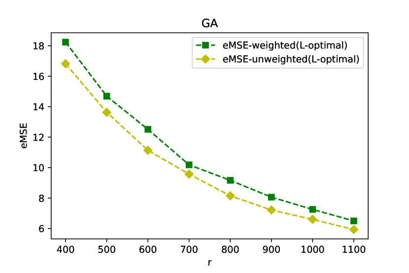
(a) GA

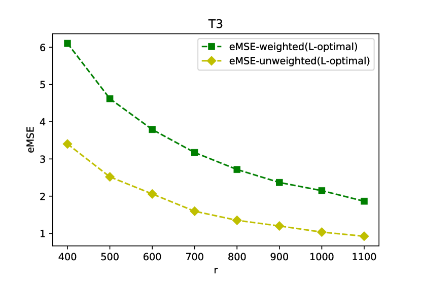
(b) T3

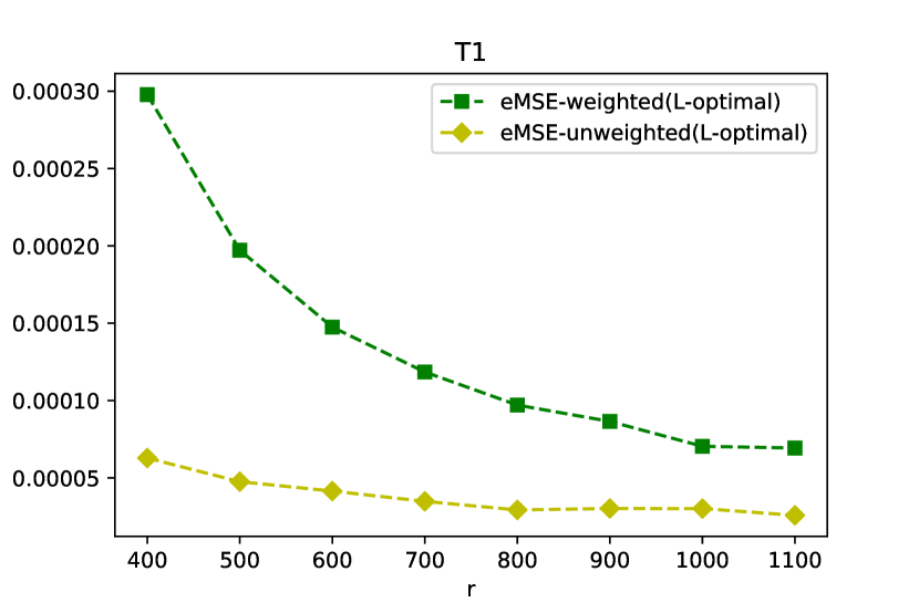
(c) T1

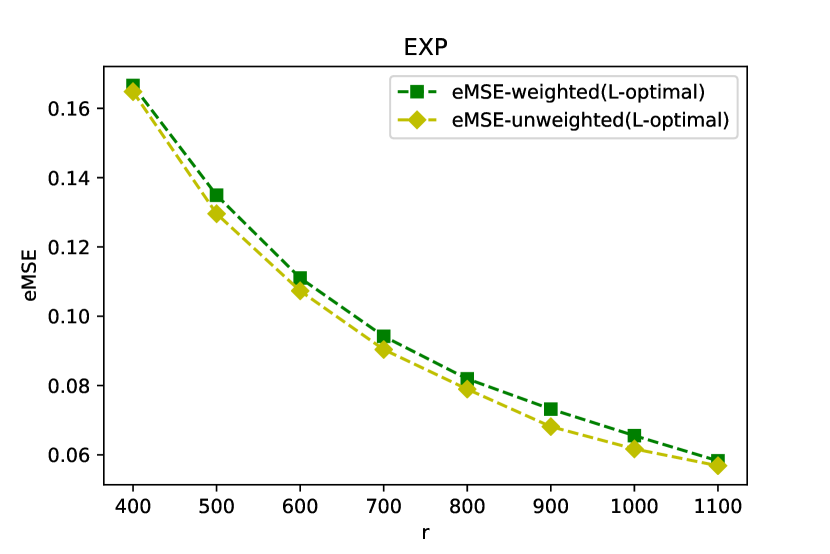
(d) EXP

Figure A.1: eMSE for different subsampe sizes $r$ for linear regression under different settings.

A.3.2 Influence of the pilot estimation

In this section, we use numerical experiments to evaluate the effect of the pilot estimation method. We use the same settings as in Section 4.1 for logistic regression and take $N=100000$. We set the pilot subsample size to be $r_{\mathrm{p}}=500$. To compare the performances of using different methods to obtain the pilot estimates, we consider the simple random sampling and the case-control sampling (Fithian & Hastie, 2014; Wang, 2019). The case-control sampling method use the following probabilities:

$$\pi_{0i}=\frac{c_{0}(1-y_{i})+c_{1}y_{i}}{n}$$

to take data points, where $c_{0}$ and $c_{1}$ are constants to balance the responses. We choose $c_{0}=\{2(1-p_{m})\}^{-1}$ and $c_{1}=(2p_{m})^{-1}$, where $p_{m}$ denotes the prior maginal probability $\mathbb{P}(y=1)$. We present the results in Figure A.2. It is seen that the eMSEs of the final subsample estimators obtained by using simple random sampling and case-control sampling as the pilot estimation method are similar for both A-optimal and L-optimal probabilities. This indicates that the influence of the methods used to obtain the pilot estimates is not significant for the setting considered.

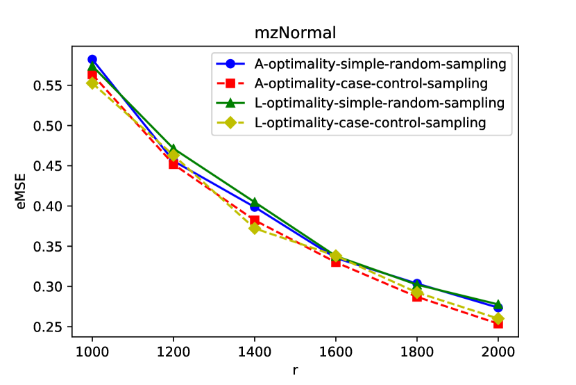
(a) mzNormal

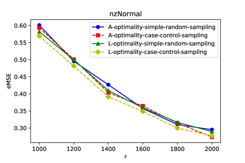
(b) nzNormal

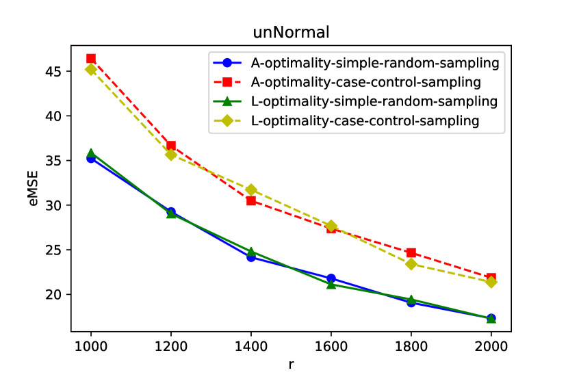
(c) unNormal

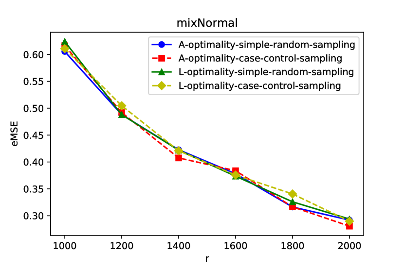
(d) mixNormal

Figure A.2: eMSE for different subsample sizes $r$ with a pilot sample size $r_{\mathrm{p}}=500$ for logistic regression under different settings and different sampling methods for pilot estimation.

References

- Ai et al. (2021) Ai, M., Yu, J., Zhang, H., & Wang, H. (2021). Optimal subsampling algorithms for big data regressions. Statistica Sinica, 31(2):749–772.
- Andrews (1988) Andrews, D. W. (1988). Laws of large numbers for dependent non-identically distributed random variables. Econometric theory, 4(3):458–467.
- Blum et al. (1958) Blum, J., Chernoff, H., Rosenblatt, M., & Teicher, H. (1958). Central limit theorems for interchangeable processes. Canad. J. Math, 10:222–229.
- Cheng et al. (2020) Cheng, Q., Wang, H., & Yang, M. (2020). Information-based optimal subdata selection for big data logistic regression. Journal of Statistical Planning and Inference, 209:112 – 122.
- Chow & Teicher (2003) Chow, Y. S. C. & Teicher, H. (2003). Probability Theory: Independence, Interchangeability, Martingales. Springer, New York.
- Davidson (1994) Davidson, J. (1994). Stochastic Limit Theory. Oxford University Press.
- Drineas et al. (2011) Drineas, P., Mahoney, M., Muthukrishnan, S., & Sarlos, T. (2011). Faster least squares approximation. Numerische Mathematik, 117:219–249.
- Drineas et al. (2006) Drineas, P., Mahoney, M. W., & Muthukrishnan, S. (2006). Sampling algorithms for regression and applications. In Proceedings of the seventeenth annual ACM-SIAM symposium on Discrete algorithm, pages 1127–1136. Society for Industrial and Applied Mathematics.
- Fithian & Hastie (2014) Fithian, W. & Hastie, T. (2014). Local case-control sampling: Efficient subsampling in imbalanced data sets. Annals of statistics, 42(5):1693.
- Hjort & Pollard (2011) Hjort, N. L. & Pollard, D. (2011). Asymptotics for minimisers of convex processes. arXiv preprint arXiv:1107.3806.
- Jakubowski (1980) Jakubowski, A. (1980). On limit theorems for sums of dependent hilbert space valued random variables. In Mathematical Statistics and Probability Theory, pages 178–187. Springer.
- Lax (2007) Lax, P. D. (2007). Linear Algebra and its Applications. Wiley, New York.
- Ma et al. (2015) Ma, P., Mahoney, M. W., & Yu, B. (2015). A statistical perspective on algorithmic leveraging. The Journal of Machine Learning Research, 16(1):861–911.
- Ma et al. (2020) Ma, P., Zhang, X., Xing, X., Ma, J., & Mahoney, M. (2020). Asymptotic analysis of sampling estimators for randomized numerical linear algebra algorithms. volume 108 of Proceedings of Machine Learning Research, pages 1026–1035, Online. PMLR.
- Mahoney (2011) Mahoney, M. W. (2011). Randomized algorithms for matrices and data. Foundations and Trends® in Machine Learning, 3(2):123–224.
- McCullagh & Nelder (1989) McCullagh, P. & Nelder, J. A. (1989). Generalized Linear Models, no. 37 in Monograph on Statistics and Applied Probability. Chapman & Hall,.
- Nie et al. (2018) Nie, R., Wiens, D. P., & Zhai, Z. (2018). Minimax robust active learning for approximately specified regression models. Canadian Journal of Statistics, 46(1):104–122.
- Pronzato & Wang (2021) Pronzato, L. & Wang, H. (2021). Sequential online subsampling for thinning experimental designs. Journal of Statistical Planning and Inference, 212:169–193.
- Wang (2019) Wang, H. (2019). More efficient estimation for logistic regression with optimal subsamples. Journal of Machine Learning Research, 20(132):1–59.
- Wang & Ma (2020) Wang, H. & Ma, Y. (2020). Optimal subsampling for quantile regression in big data. Biometrika, 108(1):99–112.
- Wang et al. (2019) Wang, H., Yang, M., & Stufken, J. (2019). Information-based optimal subdata selection for big data linear regression. Journal of the American Statistical Association, 114(525):393–405.
- Wang et al. (2018) Wang, H., Zhu, R., & Ma, P. (2018). Optimal subsampling for large sample logistic regression. Journal of the American Statistical Association, 113(522):829–844.
- Xiong & Li (2008) Xiong, S. & Li, G. (2008). Some results on the convergence of conditional distributions. Statistics & Probability Letters, 78(18):3249–3253.
- Yu et al. (2022) Yu, J., Wang, H., Ai, M., & Zhang, H. (2022). Optimal distributed subsampling for maximum quasi-likelihood estimators with massive data. Journal of the American Statistical Association, 117(537):265–276.
- Zhang & Wang (2021) Zhang, H. & Wang, H. (2021). Distributed subdata selection for big data via sampling-based approach. Computational Statistics & Data Analysis, 153:107072.
- Zhang et al. (2021) Zhang, T., Ning, Y., & Ruppert, D. (2021). Optimal sampling for generalized linear models under measurement constraints. Journal of Computational and Graphical Statistics, 30(1):106–114.