Multi-Task Dynamical Systems

Abstract

Time series datasets are often composed of a variety of sequences from the same domain, but from different entities, such as individuals, products, or organizations. We are interested in how time series models can be specialized to individual sequences (capturing the specific characteristics) while still retaining statistical power by sharing commonalities across the sequences. This paper describes the multi-task dynamical system (MTDS); a general methodology for extending multi-task learning (MTL) to time series models. Our approach endows dynamical systems with a set of hierarchical latent variables which can modulate all model parameters. To our knowledge, this is a novel development of MTL, and applies to time series both with and without control inputs. We apply the MTDS to motion-capture data of people walking in various styles using a multi-task recurrent neural network (RNN), and to patient drug-response data using a multi-task pharmacodynamic model.

Keywords: time series, dynamical systems, multi-task learning, latent variable models, sequential Bayesian inference

1 Introduction

Perhaps the most important class of time series models today are dynamical systems, which encompass a wide variety of models. Applications may be found in domains as diverse as physical modelling (see e.g. Linderman et al., 2017), drug response (e.g. White et al., 2008), public transport demand forecasting (e.g. Toqué et al., 2016), motion capture (e.g. Martinez et al., 2017), and retail sales data (e.g. Rangapuram et al., 2018) to name but a few. Since such time series data can arise from various sources (such as different people, systems, locations or organizations), each data set often comprises a variety of sequences with different characteristics. For instance, motion capture data might include different styles of walking, and healthcare data might exhibit a variety of personalized responses to the same drug. These characteristic differences often require different dynamics, which a single dynamical system is unable to provide, at least explicitly. In this paper, we describe how dynamical systems can be modified to adapt to this inter-sequence variation via the use of a set of hierarchical latent variables, thus enabling ‘personalization’ or ‘customization’ of the models.

There are two common approaches to modelling such inter-sequence variation: the most flexible option is to train an individual model per sequence (as per the graphical model in Figure 1a). An individual model can in principle capture idiosyncratic features, but suffers from overfitting and fails to exploit the regularities between the sequences in the training set. More commonly, the different sequences are pooled together to train a single dynamical system, despite the inter-sequence variation (a one-size-fits-all approach, Figure 1c). This may fail to capture the idiosyncratic features at all; a simple model such as a linear dynamical system (LDS) will learn only an average effect.

(a)

(b)

(c)

Figure 1: Comparison of approaches for modelling multiple sequences using dynamical systems with inputs $\mathbf{u}$, observations $\mathbf{y}$, hidden states $\mathbf{x}$, task variables $\mathbf{z}$; and dynamical system parameters ${\bm{\theta}}$, multi-task parameters ${\bm{\phi}}$. Panels show (a) a single task approach, where each sequence is learned separately; (b) the multi-task dynamical system; (c) the pooled approach.

In contrast to these approaches, we aim to learn a family of dynamical systems that is consistent with the sequences in the training set. Each training sequence is given a bespoke model from the ‘sequence family’, but this family exploits the regularities observed across all sequences, which can substantially reduce overfitting. We achieve this via use of a set of hierarchical latent variables, similar to the approach used in multi-task learning for iid data, now with each sequence treated as a task. We hence call this approach the multi-task dynamical system (MTDS). The MTDS learns a low dimensional manifold in parameter space, indexed by a latent code $\mathbf{z}\in{\mathcal{Z}}$, which corresponds to the specialization of each sequence model. See Figure 1b for a graphical model.

The choice of a low dimensional manifold enables the MTDS to determine directions in parameter space with respect to which the parameters ${\bm{\theta}}\in\Theta$ need not change, sharing strength across sequences. This avoids considering directions in $\Theta$ which result in unlikely or uncharacteristic predictions, as well as ignoring so-called ‘sloppy directions’ (Transtrum et al., 2011), which can add great complexity to inference, with little benefit in terms of fit or generalization. But it can also find the key direction(s) of variability in $\Theta$ between training sequences. As a simple example, consider sequences generated from the family of $d$th order linear ODEs. Such sequences may vary in terms of oscillation frequencies, magnitude, half life to an input impulse, etc. A good approximation of these sequences is possible via a $d$-dimensional LDS (see e.g. Aström and Murray, 2010, §2.2, §5.3), but while the ODE has $d{+}1$ degrees of freedom, the LDS has ${\mathcal{O}}(d^{2})$ in general. An MTDS approach can learn the relevant $d{+}1$ degrees of freedom of the LDS in $\Theta$ simply by training on example sequences. For an example of this, see §4, Bird (2021).

Unlike previous efforts to customize time series models, our MTDS construction allows application to general classes of dynamical systems. This is available due to our choice of learning an arbitrary manifold over all the model parameters (both system and emission), rather than being constrained to pre-determined parameter sets (see the related work in Section 3). This allows the MTDS to model variability in observation space (such as magnitude or offset), as well as different responses to inputs, different sensitivity to initial conditions, and differences in dynamic evolution. The MTDS can thus be applied to classical ARMA models, state space models, and modern recurrent neural networks (RNNs).

The MTDS provides user visibility of the task specialization, as well as the ability to control it directly if desired, via use of the hierarchical latent variable $\mathbf{z}$. This stands in contrast to a RNN approach, which also has the flexibility to model inter-sequence variation, but does so in an implicit and opaque ‘black-box’ manner. This prohibits interpretability and end-user control, but can also suffer from mode drift where the personalization erroneously changes over time. For example, in Ghosh et al. (2017) a RNN generates a motion capture (mocap) sequence which performs an unprompted transition from walking to drinking. Our contributions with respect to such end-user control will be explored further in the empirical work, especially in Section 4.

In this paper we propose the MTDS, which endows dynamical systems with the ability to adapt to inter-sequence variation. Our contributions go beyond existing work by: (i) allowing the full adaptation of all parameters of general dynamical systems via use of a learned nonlinear manifold; (ii) describing efficient general purpose forms of learning and inference; (iii) performing in-depth experimental studies using data from human locomotion data and medical time series; and (iv) investigating the advantages of our proposal, which—compared to standard single-task and pooled approaches—include substantial improvements in data efficiency, robustness to dataset-shift, user control (which may be used for style transfer, for example), and online customization of interpretable models.

In what follows, Section 2 introduces the MTDS, including a discussion of learning and inference, and Section 3 provides an overview of related work. We provide two in-depth case studies: a multi-task RNN in Section 4 for a mocap data application, and a multi-task pharmacodynamic model in Section 5 for personalized drug response modelling.

2 The Multi-Task Dynamical System

In this section, we define the multi-task dynamical system (Section 2.1) and provide methods for learning (Section 2.2) and inference (Section 2.3).

2.1 Definition

Consider a collection of $N$ input-output sequences $\mathcal{D}=\big{\{}\mkern 2.0mu(\mkern 1.0mu\mathbf{u}_{1\mathrel{\mathop{\mathchar 58\relax}}T_{i}}^{(i)},\;\mathbf{y}_{1\mathrel{\mathop{\mathchar 58\relax}}T_{i}}^{(i)}\mkern 1.0mu)\mkern 2.0mu\big{\}}_{i=1}^{N}$ consisting of inputs and outputs respectively, where $T_{i}$ is the length of sequence $i$. Each sequence $i$ is described by a different dynamical system with state variables $\mathbf{x}_{t}^{(i)}\in{\mathcal{X}}$, $t=1,\ldots,T_{i}$ whose parameter ${\bm{\theta}}^{(i)}\in\Theta$ depends on the hierarchical latent variable $\mathbf{z}^{(i)}\in{\mathcal{Z}}$. See Figure 1(b) for a graphical model. The MTDS is defined by the equations:

$${\bm{\theta}}^{(i)} \;=\;\mathbf{h}_{{\bm{\phi}}}(\mathbf{z}^{(i)}),\quad\mathbf{z}^{(i)}\;\sim\;p(\mathbf{z})$$ (1)

$$\mathbf{x}_{t}^{(i)} \;\sim\;p(\mathbf{x}\mid\;\mathbf{x}_{t-1}^{(i)},\;\mathbf{u}_{t}^{(i)},\;{\bm{\theta}}^{(i)}),$$ (2)

$$\mathbf{y}_{t}^{(i)} \;\sim\;p(\mathbf{y}\mid\;\mathbf{x}_{t}^{(i)},\;\mathbf{u}_{t}^{(i)},\;{\bm{\theta}}^{(i)}),$$ (3)

for $t=1,\ldots,T_{i}$ for each $i=1,\ldots,N$, where eq. (2) represents the dynamic evolution and is sometimes referred to as the system equation, and eq. (3) is the emission equation. In this paper we assume $\mathbf{x}_{0}\vcentcolon=\mathbf{0}$, and ${\mathcal{Z}}=\mathbb{R}^{k}$ which the vector-valued function $\mathbf{h}_{{\bm{\phi}}}(\cdot)$ transforms to conformable model parameters ${\bm{\theta}}\in\mathbb{R}^{d}$. By restricting the parameter manifold to $k\ll d$ dimensions, eqs. (1-3) result in a multi-task model rather than simply a hierarchical model.

The MTDS model thus requires the specification of three key quantities:

1. The base model (eqs. 2-3), such as a LDS or RNN.

2. The dimensions of ${\bm{\theta}}$ that depend on the latent variable $\mathbf{z}$ (for example, one might choose the emissions (eq. 3) to be constant wrt. $\mathbf{z}$, or to modulate only the offset/bias terms of eqs. (2) and (3) wrt. $\mathbf{z}$).

3. The choice of prior $p({\bm{\theta}})$, that is, the choice of distribution $p(\mathbf{z})$ and transformation $\mathbf{h}_{{\bm{\phi}}}$.

We restrict our focus to deterministic state dynamical systems which simplifies the exposition and is motivated by our focus on longer term prediction. In our experience we have found deterministic models generally outperform stochastic state models for long-term prediction, see also (for example) Bengio et al. (2015); Chiappa et al. (2017), and additional comments in Appendix A.2. Some example choices of base model are elaborated upon in Sections 4.2 and 5.2.1. Note that where the dynamics of eq. (2) are linear, some care must be given to ensuring the stability of the system (see Bird, 2021, §3.2).

The choice of prior $p({\bm{\theta}})$ considered in this paper is a (nonlinear) factor analysis model, described by:

$${\bm{\theta}}\,=\,\mathbf{h}_{{\bm{\phi}}}(\mathbf{z}),\qquad\qquad p(\mathbf{z})\,=\,\mathcal{N}\left(0,I\right),$$ (4)

where $\mathbf{h}_{{\bm{\phi}}}$ is some deterministic function. An affine $\mathbf{h}_{{\bm{\phi}}}$ may be useful where interpretability is important, or base models are highly flexible. Non-affine functions, such as multilayer perceptrons (cf. Kingma and Welling, 2014; Rezende et al., 2014) have proved to be important when using relatively inflexible base models such as LDSs. See Appendix A.1 for some additional considerations.

2.2 Learning

The parameters ${\bm{\phi}}$ of an MTDS can be learned from a data set $\mathcal{D}\vcentcolon=\{Y^{(i)},U^{(i)}\}_{i=1}^{N}$, defining $Y\vcentcolon=\mathbf{y}_{1\mathrel{\mathop{\mathchar 58\relax}}T},\;U\vcentcolon=\mathbf{u}_{1\mathrel{\mathop{\mathchar 58\relax}}T}$ to reduce the notational burden. We can learn the parameters via maximum marginal likelihood:

$${\bm{\phi}}^{*}\; =\;\arg\max_{\bm{\phi}}\,\sum_{i=1}^{N}\log p(Y^{(i)}\,|\,U^{(i)},{\bm{\phi}}),$$ (5)

where

$$\log p(Y\,|\,U,{\bm{\phi}})\; =\;\log\int_{\mathcal{Z}}p(Y\,|\,U,\mathbf{h}_{{\bm{\phi}}}(\mathbf{z}))\,p(\mathbf{z})\operatorname{d\!}\mathbf{z}.$$ (6)

The first term in this integrand,

$$p(Y\,|\,U,\mathbf{h}_{{\bm{\phi}}}(\mathbf{z}))\; =\;\int_{{\mathcal{X}}^{T}}p(Y\,|\,X,U,\mathbf{h}_{{\bm{\phi}}}(\mathbf{z}))\,p(X|U,\mathbf{h}_{{\bm{\phi}}}(\mathbf{z}))\operatorname{d\!}X$$ (7)

is generally intractable for stochastic dynamics (with notable exceptions of discrete and linear-Gaussian models). In this paper we restrict our attention to deterministic state models (see above, and discussion in Appendix A.2), but eq. (7) may be approached via existing methods such as variational methods (e.g. Goyal et al., 2017; Miladinović et al., 2019) or a Monte Carlo objective (MCO) e.g. Maddison et al. (2017); Le et al. (2018); Naesseth et al. (2018).

We then turn to the integral in equation (6). Generally, this integral is also unavailable in closed form, and must be approximated. We make use of a variational approach, optimizing the Evidence Lower Bound (ELBO), $\mathcal{L}(Y,U;{\bm{\phi}},{\bm{\lambda}})\,\leq\,\log p(Y\,|\,U,{\bm{\phi}})$, defined by:

$$\mathcal{L}(Y,U;{\bm{\phi}},{\bm{\lambda}}) \,=\,\mathbb{E}_{\mathchoice{q_{\raisebox{-2.0pt}{\scalebox{0.7}{$\displaystyle{\bm{\lambda}}$}}}}{q_{\raisebox{-2.0pt}{\scalebox{0.7}{$\textstyle{\bm{\lambda}}$}}}}{q_{\raisebox{-2.0pt}{\scalebox{0.7}{$\scriptstyle{\bm{\lambda}}$}}}}{q_{\raisebox{-2.0pt}{\scalebox{0.7}{$\scriptscriptstyle{\bm{\lambda}}$}}}}(\mathbf{z}\,|\,Y,U)}\left[\log p(Y\,|\,U,\mathbf{h}_{{\bm{\phi}}}(\mathbf{z}))\right]-\text{KL}\left(\,\mathchoice{q_{\raisebox{-2.0pt}{\scalebox{0.7}{$\displaystyle{\bm{\lambda}}$}}}}{q_{\raisebox{-2.0pt}{\scalebox{0.7}{$\textstyle{\bm{\lambda}}$}}}}{q_{\raisebox{-2.0pt}{\scalebox{0.7}{$\scriptstyle{\bm{\lambda}}$}}}}{q_{\raisebox{-2.0pt}{\scalebox{0.7}{$\scriptscriptstyle{\bm{\lambda}}$}}}}(\mathbf{z}\,|\,Y,U)\,\,\middle\|\,\,p(\mathbf{z})\,\right),$$ (8)

where KL is the Kullback-Leibler divergence and $\mathchoice{q_{\raisebox{-2.0pt}{\scalebox{0.7}{$\displaystyle{\bm{\lambda}}$}}}}{q_{\raisebox{-2.0pt}{\scalebox{0.7}{$\textstyle{\bm{\lambda}}$}}}}{q_{\raisebox{-2.0pt}{\scalebox{0.7}{$\scriptstyle{\bm{\lambda}}$}}}}{q_{\raisebox{-2.0pt}{\scalebox{0.7}{$\scriptscriptstyle{\bm{\lambda}}$}}}}(\mathbf{z}\,|\,Y,U)$ is an approximate posterior for $\mathbf{z}$. The lower bound $\sum_{i=1}^{N}\mathcal{L}(Y^{(i)},U^{(i)};{\bm{\phi}},{\bm{\lambda}})$ may then be optimized via reparameterization (Kingma and Welling, 2014; Rezende et al., 2014), with minibatches of size $N_{\textrm{batch}}<N$. We will generally consider $\mathchoice{q_{\raisebox{-2.0pt}{\scalebox{0.7}{$\displaystyle{\bm{\lambda}}$}}}}{q_{\raisebox{-2.0pt}{\scalebox{0.7}{$\textstyle{\bm{\lambda}}$}}}}{q_{\raisebox{-2.0pt}{\scalebox{0.7}{$\scriptstyle{\bm{\lambda}}$}}}}{q_{\raisebox{-2.0pt}{\scalebox{0.7}{$\scriptscriptstyle{\bm{\lambda}}$}}}}(\mathbf{z}\,|\,Y,U)=\,\mathcal{N}\left(\mathchoice{\bm{\mu}_{\raisebox{-0.8pt}{\scalebox{0.7}{$\displaystyle{\bm{\lambda}}$}}}}{\bm{\mu}_{\raisebox{-0.8pt}{\scalebox{0.7}{$\textstyle{\bm{\lambda}}$}}}}{\bm{\mu}_{\raisebox{-0.8pt}{\scalebox{0.7}{$\scriptstyle{\bm{\lambda}}$}}}}{\bm{\mu}_{\raisebox{-0.8pt}{\scalebox{0.7}{$\scriptscriptstyle{\bm{\lambda}}$}}}}(Y,U),\,\mathchoice{\mathbf{s}_{\raisebox{-1.5pt}{\scalebox{0.7}{$\displaystyle{\bm{\lambda}}$}}}}{\mathbf{s}_{\raisebox{-1.5pt}{\scalebox{0.7}{$\textstyle{\bm{\lambda}}$}}}}{\mathbf{s}_{\raisebox{-1.5pt}{\scalebox{0.7}{$\scriptstyle{\bm{\lambda}}$}}}}{\mathbf{s}_{\raisebox{-1.5pt}{\scalebox{0.7}{$\scriptscriptstyle{\bm{\lambda}}$}}}}(Y,U)\right)$, where $\mathchoice{\bm{\mu}_{\raisebox{-0.8pt}{\scalebox{0.7}{$\displaystyle{\bm{\lambda}}$}}}}{\bm{\mu}_{\raisebox{-0.8pt}{\scalebox{0.7}{$\textstyle{\bm{\lambda}}$}}}}{\bm{\mu}_{\raisebox{-0.8pt}{\scalebox{0.7}{$\scriptstyle{\bm{\lambda}}$}}}}{\bm{\mu}_{\raisebox{-0.8pt}{\scalebox{0.7}{$\scriptscriptstyle{\bm{\lambda}}$}}}}$, $\mathchoice{\mathbf{s}_{\raisebox{-1.5pt}{\scalebox{0.7}{$\displaystyle{\bm{\lambda}}$}}}}{\mathbf{s}_{\raisebox{-1.5pt}{\scalebox{0.7}{$\textstyle{\bm{\lambda}}$}}}}{\mathbf{s}_{\raisebox{-1.5pt}{\scalebox{0.7}{$\scriptstyle{\bm{\lambda}}$}}}}{\mathbf{s}_{\raisebox{-1.5pt}{\scalebox{0.7}{$\scriptscriptstyle{\bm{\lambda}}$}}}}$ are either inference networks (as e.g. Fabius and van Amersfoort, 2015) or optimized directly as parameters. These variational parameters may of direct interest (e.g. for visualization), but may alternatively be an auxiliary artifact to be discarded after optimization. In all our experiments, we chose the $\mathchoice{\mathbf{s}_{\raisebox{-1.5pt}{\scalebox{0.7}{$\displaystyle{\bm{\lambda}}$}}}}{\mathbf{s}_{\raisebox{-1.5pt}{\scalebox{0.7}{$\textstyle{\bm{\lambda}}$}}}}{\mathbf{s}_{\raisebox{-1.5pt}{\scalebox{0.7}{$\scriptstyle{\bm{\lambda}}$}}}}{\mathbf{s}_{\raisebox{-1.5pt}{\scalebox{0.7}{$\scriptscriptstyle{\bm{\lambda}}$}}}}(Y,U)$ to be diagonal matrices.

We can optimize the ELBO in eq. (8) via access to $\nabla_{\bm{\phi}}\log p(Y\,|\,U,\mathbf{h}_{{\bm{\phi}}}(\mathbf{z}))$ which we assume to be available (typically via use of an automatic differentiation framework). For our implementation, see Appendix A.3. A tighter lower bound can be achieved using related ideas, for example, using the bound introduced by the importance weighted autoencoder (IWAE) of Burda et al. (2016). Where $p(Y\,|\,U,\mathbf{h}_{{\bm{\phi}}}(\mathbf{z}))$ is a powerful base model such as an RNN, the ELBO is well-known to exhibit latent collapse: a higher value of the ELBO can be achieved if the model is able to avoid using the latent $\mathbf{z}$ (e.g. Chen et al., 2017). In our experiments we used a form of KL annealing (Bowman et al., 2016) to avoid this.

2.3 Inference of $\mathbf{z}$

A key quantity for predicting future observations is the posterior predictive distribution. For an unseen test sequence $\{Y^{\prime},U^{\prime}\}$, the posterior predictive distribution is

$$p(\mathbf{y}_{t+1\mathrel{\mathop{\mathchar 58\relax}}T}^{\prime}\,|\,\mathbf{y}_{1\mathrel{\mathop{\mathchar 58\relax}}t}^{\prime},\,\mathbf{u}_{1\mathrel{\mathop{\mathchar 58\relax}}T}^{\prime})\,=\,\int_{\mathcal{Z}}p(\mathbf{y}_{t+1\mathrel{\mathop{\mathchar 58\relax}}T}^{\prime}\,|\,\mathbf{u}_{1\mathrel{\mathop{\mathchar 58\relax}}T}^{\prime},\,\mathbf{z})\,p(\mathbf{z}\,|\,\mathbf{y}_{1\mathrel{\mathop{\mathchar 58\relax}}t}^{\prime},\,\mathbf{u}_{1\mathrel{\mathop{\mathchar 58\relax}}t}^{\prime})\operatorname{d\!}\mathbf{z},$$ (9)

usually estimated via Monte Carlo. We must therefore have access to the posterior $p(\mathbf{z}\,|\,\mathbf{y}_{1\mathrel{\mathop{\mathchar 58\relax}}t}^{\prime},\,\mathbf{u}_{1\mathrel{\mathop{\mathchar 58\relax}}t}^{\prime})$. This may sometimes be available as an artifact of the variational optimization, but in general we cannot assume that the variational distributions $\mathchoice{q_{\raisebox{-2.0pt}{\scalebox{0.7}{$\displaystyle{\bm{\lambda}}$}}}}{q_{\raisebox{-2.0pt}{\scalebox{0.7}{$\textstyle{\bm{\lambda}}$}}}}{q_{\raisebox{-2.0pt}{\scalebox{0.7}{$\scriptstyle{\bm{\lambda}}$}}}}{q_{\raisebox{-2.0pt}{\scalebox{0.7}{$\scriptscriptstyle{\bm{\lambda}}$}}}}$ generalize to $t>T$ or to out-of-sample sequences. In this section we consider a more general method of inference.

Inferring $\mathbf{z}$ is possible via a wide variety of variational or Monte Carlo approaches. However, given the sequential nature of the model, it is natural to consider exploiting the posterior at time $t$ for calculating the posterior at time $t{+}1$. Bayes’ rule implies an update of the following form:

$$p(\mathbf{z}\,|\,\mathbf{y}_{1\mathrel{\mathop{\mathchar 58\relax}}t+1}^{\prime},\mathbf{u}_{1\mathrel{\mathop{\mathchar 58\relax}}t+1}^{\prime})\;\propto\;p(\mathbf{y}_{t+1}^{\prime}\,|\,\mathbf{y}_{1\mathrel{\mathop{\mathchar 58\relax}}t}^{\prime},\mathbf{u}_{1\mathrel{\mathop{\mathchar 58\relax}}t+1}^{\prime},\mathbf{h}_{{\bm{\phi}}}(\mathbf{z}))\,p(\mathbf{z}\,|\,\mathbf{y}_{1\mathrel{\mathop{\mathchar 58\relax}}t}^{\prime},\mathbf{u}_{1\mathrel{\mathop{\mathchar 58\relax}}t}^{\prime}),$$ (10)

following the conditional independence assumptions of the MTDS. This update (in principle) incorporates the information learned at time $t$ in an optimal way. We are interested in inferential methods which can exploit this prior information efficiently. Below we discuss existing work using both Monte Carlo (MC) and variational inference, before discussing our preferred approach in Sec. 2.3.3 using adaptive importance sampling.

2.3.1 Monte Carlo Inference

A gold standard of inference over $\mathbf{z}$ may be the No U-Turn Sampler (NUTS) of Hoffman and Gelman (2014) (a form of Hamiltonian Monte Carlo), provided $k$ is not too large and efficiency is not a concern. However, eq. (10) casts doubt on the use of Markov Chain Monte Carlo (MCMC) methods, since it is not obvious how to incorporate at time $t{+}1$ the samples of $\mathbf{z}$ obtained at time $t$. Perhaps a more relevant approach is Sequential Monte Carlo (SMC, e.g. Doucet et al., 2000) which is designed for use in a sequential context. Unfortunately, naïve use of SMC (particle filtering) will result in severe particle depletion over time. To see this, let the posterior after time $t$ be approximated as $p(\mathbf{z}\,|\,\mathbf{y}_{1\mathrel{\mathop{\mathchar 58\relax}}t}^{\prime},\mathbf{u}_{1\mathrel{\mathop{\mathchar 58\relax}}t}^{\prime})=\frac{1}{M}\sum_{m=1}^{M}w_{m}\delta(\mathbf{z}-\mathbf{z}_{m})$. Then the updated posterior at time $t+1$ will be:

$$p(\mathbf{z}\,|\,\mathbf{y}_{1\mathrel{\mathop{\mathchar 58\relax}}t+1}^{\prime},\mathbf{u}_{1\mathrel{\mathop{\mathchar 58\relax}}t+1}^{\prime}) \;\propto\;\frac{1}{M}\sum_{m=1}^{M}w_{m}p(\mathbf{y}_{t+1}^{\prime}\,|\,\mathbf{y}_{1\mathrel{\mathop{\mathchar 58\relax}}t}^{\prime},\mathbf{u}_{t+1}^{\prime},\mathbf{h}_{{\bm{\phi}}}(\mathbf{z}))\delta(\mathbf{z}-\mathbf{z}_{m}),$$

$$\Rightarrow p(\mathbf{z}\,|\,\mathbf{y}_{1\mathrel{\mathop{\mathchar 58\relax}}t+1}^{\prime},\mathbf{u}_{1\mathrel{\mathop{\mathchar 58\relax}}t+1}^{\prime}) \;=\;\frac{1}{M}\sum_{m=1}^{M}\tilde{w}_{m}\delta(\mathbf{z}-\mathbf{z}_{m}),$$

where $\tilde{w}_{m}=\frac{w_{m}p(\mathbf{y}_{t+1}^{\prime}\,|\,\mathbf{y}_{1\mathrel{\mathop{\mathchar 58\relax}}t}^{\prime},\mathbf{u}_{t+1}^{\prime},\mathbf{h}_{{\bm{\phi}}}(\mathbf{z}_{m}))}{\sum_{j=1}^{M}w_{j}p(\mathbf{y}_{t+1}^{\prime}\,|\,\mathbf{y}_{1\mathrel{\mathop{\mathchar 58\relax}}t}^{\prime},\mathbf{u}_{t+1}^{\prime},\mathbf{h}_{{\bm{\phi}}}(\mathbf{z}_{j}))}$, simply a re-weighting of existing particles. The number of particles with significant weights $w_{m}$ will reduce quickly over time (see e.g. Doucet et al., 2000, sec. II.C). But since the model is static with respect to $\mathbf{z}$ (see Chopin, 2002), there is no dynamic process to ‘jitter’ the $\{\mathbf{z}_{m}\}$ as in a typical particle filter, and hence a resampling step cannot improve diversity.

Chopin (2002) discusses two related solutions: firstly using ‘rejuvenation steps’ (cf. Gilks and Berzuini, 2001) which applies a Markov transition kernel to each particle. The downside to this approach is the requirement to run until convergence; and the diagnosis thereof, which may take a long time. The second alternative given is to sample from a ‘fixed’ (or global) proposal distribution (accepting a move with the usual Metropolis-Hastings probability) for which convergence is more easily monitored. This introduces a further difficulty, however, of appropriately tuning the proposal distribution. Neither option appears practical as an efficient inner step for iterations of eq. (10).

2.3.2 Variational Inference

Variational inference (VI) considers a parametric approximation to the posterior $p(\mathbf{z}\,|\,\mathbf{y}_{1\mathrel{\mathop{\mathchar 58\relax}}t},\,\mathbf{u}_{1\mathrel{\mathop{\mathchar 58\relax}}t})$; variational approaches may not be statistically consistent, but they can generally obtain an approximation more quickly than MC methods. A well-known approach to problems with the structure of eq. (10) is assumed density filtering (ADF, see e.g. Opper and Winther, 1998). For each $t$, ADF performs the Bayesian update and then projects the posterior into a parametric family ${\mathcal{Q}}$. The projection is done with respect to the reverse KL Divergence, i.e. $q_{t+1}=\arg\min_{q\in{\mathcal{Q}}}\text{KL}\left(p(\mathbf{z}\,|\,\mathbf{y}_{1\mathrel{\mathop{\mathchar 58\relax}}t+1}^{\prime},\mathbf{u}_{1\mathrel{\mathop{\mathchar 58\relax}}t+1}^{\prime})\,\,\middle\|\,\,q\right)$. Intuitively, the projection finds an ‘outer approximation’ of the true posterior, avoiding the ‘mode seeking’ behaviour of the usual forward KL, which is particularly problematic if it attaches to the wrong mode.

Clearly the performance of ADF depends crucially on the choice of ${\mathcal{Q}}$. Unfortunately, where ${\mathcal{Q}}$ is expressive enough to capture a good approximation, the optimization problem will usually be challenging, typically requiring a stochastic gradient approach, resulting in an expensive inner loop. Furthermore, when the changes from $q_{t}$ to $q_{t+1}$ are relatively small, the gradient signal will be weak, which may result in misdiagnosed convergence and a consequent accumulation of error over increasing $t$. Some improvements are possible, such as re-use of stale gradients (Tomasetti et al., 2019) or standard variance reduction techniques. Nevertheless, given the possible inefficiencies of stochastic gradient approaches, compounded errors, and inaccuracies derived from ${\mathcal{Q}}$, ADF may be considered unreliable for general use.

2.3.3 An Adaptive Importance Sampling Approach

Having discussed an overview of possible options, we now introduce our proposed method: a sequential application of adaptive importance sampling (IS). This blends the advantages of both MC and VI methods by using a parametric posterior approximation $q_{\textrm{prop}}$ which is fitted via Monte Carlo methods, specifically, adaptive IS (see below). The parametric posterior generates the required diversity in samples without resorting to MCMC moves, and the use of IS accelerates convergence and avoids the compounded errors of ADF. The key quantity for IS is the proposal distribution $q_{\textrm{prop}}$: IS will not perform well unless $q_{\textrm{prop}}$ is well-matched to the target distribution. Our observation is that the natural annealing properties of the filtering distributions (eq. 10) allow a slow and reliable adaptation of the proposal distribution; it has proved highly effective in our applied work.

The target distribution (the posterior) can be multimodal and highly non-Gaussian, but in practice can usually be well approximated by a Gaussian mixture model (GMM). We have found this to be a good choice for $q_{\textrm{prop}}$ in our experiments. At each time $t$, the proposal distribution $q_{\textrm{prop}}$ is improved over $N_{\scriptscriptstyle\textrm{AdaIS}}$ iterations using adaptive importance sampling (AdaIS), described for mixture models in Cappé et al. (2008). We briefly review the methodology for a single target distribution $p_{*}$. Let the AdaIS procedure at the $n$th iteration fit the proposal:

$$q_{\textrm{prop}}^{n}(\mathbf{z})\;\vcentcolon=\;\sum_{j=1}^{J}\alpha_{j}^{n}\mathcal{N}\left(\mathbf{z}\,\mid\,\bm{\mu}_{j}^{n},\,\Sigma_{j}^{n}\right),$$ (11)

with $\alpha_{j}^{n}\in\mathbb{R}_{+}$ such that $\sum_{j=1}^{J}\alpha_{j}^{n}=1$ (for all $n$). For each iteration $n$, perform:

$$\mathbf{z}_{m}\, \sim\,q_{\textrm{prop}}^{n-1},\quad m=1,\dotsc,M\qquad\quad (\textrm{sample})$$

$$\tilde{w}_{m}\, \propto\,p_{*}(\mathbf{z}_{m})/q_{\textrm{prop}}^{n-1}(\mathbf{z}_{m}),\quad m=1,\dotsc,M\qquad\quad (\textrm{calculate weights})$$

(where $q_{\textrm{prop}}^{0}$ is the prior). The $n$th proposal distribution $q_{\textrm{prop}}^{n}$ is then fitted to the resulting empirical distribution $\sum_{m=1}^{M}\tilde{w}_{m}\delta(\mathbf{z}-\mathbf{z}_{m})$, estimating $\{\alpha_{j}^{n},\bm{\mu}_{j}^{n},\Sigma_{j}^{n}\}_{j=1}^{J}$ via weighted Expectation Maximization (see Cappé et al., 2008, for details). We can monitor the effective sample size (ESS, see ch. 9, Owen, 2013) every iteration to understand the quality of $q_{\textrm{prop}}$, and stop once the ESS has reached a certain threshold $M_{\textrm{ess}}$, or when $n=N_{\scriptscriptstyle\textrm{AdaIS}}$; see Algorithm 1.

Result: Approximate posteriors $\{q_{t}\}_{t=1}^{T}$

Inputs: $\mathbf{y}_{1\mathrel{\mathop{\mathchar 58\relax}}T}^{\prime},\,\mathbf{u}_{1\mathrel{\mathop{\mathchar 58\relax}}T}^{\prime},\,{\bm{\phi}},\,M,\,M_{\textrm{ess}},\,N_{\scriptscriptstyle\textrm{AdaIS}},\,J$

$q_{0}\leftarrow p(\mathbf{z})$

for $t=1\mathrel{\mathop{\mathchar 58\relax}}T$ do

       $\textrm{ess}\leftarrow 0$

       $q_{\textrm{prop}}^{0}\leftarrow q_{t-1}$

       for $n=1\mathrel{\mathop{\mathchar 58\relax}}\textrm{$N_{\scriptscriptstyle\textrm{AdaIS}}$}$ do

             for m = 1:M do

                   $\mathbf{z}_{m}\,\sim\,q_{\textrm{prop}}^{n-1}$

                   $w_{m}\,\leftarrow\,\frac{p(\mathbf{y}_{1\mathrel{\mathop{\mathchar 58\relax}}t}^{\prime}\,|\,\mathbf{u}_{1\mathrel{\mathop{\mathchar 58\relax}}t}^{\prime},\mathbf{h}_{{\bm{\phi}}}(\mathbf{z}_{m}))p(\mathbf{z})}{q_{\textrm{prop}}^{n-1}(\mathbf{z}_{m})}$

                  

             end for

            $\tilde{w}_{m}\,\leftarrow\,\frac{w_{m}}{\sum_{\ell=1}^{M}w_{\ell}},\enskip m=1,\dotsc,M$

             $q_{\textrm{prop}}^{n}\leftarrow\textrm{WeightedEM}\left(\{\mathbf{z}_{m}\}_{m=1}^{M},\{\tilde{w}_{m}\}_{m=1}^{M},J;\,\,{\footnotesize\textrm{init}}=q_{\textrm{prop}}^{n-1}\right)$

             $\textrm{ess}\,\leftarrow\,\textrm{EffectiveSampleSize}\left(\{\tilde{w}_{m}\}_{m=1}^{M}\right)$

             if $\textrm{ess}>\textrm{$M_{\textrm{ess}}$}$ then

                  break

             end if

            

       end for

      $q_{t}\leftarrow q_{\textrm{prop}}^{n}$

end for

Algorithm 1 Filtered inference via Iterated AdaIS.

In our sequential setting, we fit a sequence of proposal distributions $q_{1},q_{2},\ldots,q_{T}$, with each proposal $q_{t}$ being tuned via AdaIS (using up to $N_{\scriptscriptstyle\textrm{AdaIS}}$ adaptations), and $q_{t-1}$ forming the prior for $q_{t}$. (We can define $q_{0}\vcentcolon=p(\mathbf{z})$ for the MTDS.) The method is thus able to make use of the previous posterior without suffering from accumulated errors, and the AdaIS updates benefit from the fast initial convergence of the EM algorithm (see e.g. Xu and Jordan, 1996). The method is more challenging in the case where $p_{*}$ is intractable, but it can be achieved by integrating ideas from Chopin et al. (2013), for example. Typically only a small number of AdaIS iterations are required (usually $N_{\scriptscriptstyle\textrm{AdaIS}}\leq 5$ for our problems), rendering the procedure substantially faster than MCMC moves—and by avoiding stochastic gradients—substantially faster than variational approaches. Finally, we have found the use of low-discrepancy MC samples such as Sobol sequences helpful in reducing sampling variance and further speeding convergence when drawing samples from each $q_{\textrm{prop}}^{n}$.

Application of adaptive importance sampling to sequential problems with static latent variables such as eq. (10) is a novel development as far as we are aware, and it has proved superior in our experiments (in terms of speed, accuracy and robustness) to the alternative approaches discussed above. The viability of this approach is perhaps questionable for larger values of $k$ (we use $k\leq 10$), but it is unclear whether larger latent spaces will be commonplace. Recall that $k$ refers to the degrees of freedom of the model family rather than the models themselves, which can have many orders of magnitude more parameters. For relatively small deterministic LDS models, and $k=4$, inference has taken ${\mathcal{O}}(\textrm{100ms})$ on a standard laptop per posterior $q_{t}$, and one may choose to thin the sequence of posteriors to multiples of $\upsilon$ steps ($t=\upsilon,2\upsilon,3\upsilon,\ldots$) rather than every step. An empirical study evaluating the MTDS on synthetic data using the AdaIS algorithm can be found in Chapter 4 of Bird (2021).

3 Related Work

Multi-task learning itself is a large and varied area of machine learning. The goal of MTL is to share statistical strength between models, which is achieved in classic work by sharing parameter sets (Caruana, 1998), clustering tasks (Bakker and Heskes, 2003) or learning a low-dimensional subspace prior over parameters (Ando and Zhang, 2005). Our approach is most similar to Ando and Zhang (2005), although we use a more flexible prior, and crucially apply the hierarchical prior to time-structured problems via dynamical systems. There is relatively little work directly extending MTL approaches to dynamical systems, but ‘families’ of time series data are common and hence have attracted a variety of approaches in different fields including machine learning and statistics. We provide a review of some relevant work below.

Supervised Adaptation:

Probably the simplest form of MTL for time series involves the case where side information, $\bm{\zeta}$, is available, perhaps via demographics, or other task descriptions. For RNNs, this is commonly exploited in two ways: $\bm{\zeta}$ can be used to customize the $\mathbf{x}_{0}$ (‘initial state customization’) or appended to the inputs for each $t$ (‘bias customization’), see Goodfellow et al. (2016, §10.2.4). In the latter case we use the phrase ‘bias customization‘, since by appending the task variable to each input $\tilde{\mathbf{u}}_{t}\leftarrow[\mathbf{u}_{t}^{\mkern-1.5mu\mathsf{T}},\bm{\zeta}^{\mkern-1.5mu\mathsf{T}}]^{\mkern-1.5mu\mathsf{T}}$ for each $t$, a RNN cell takes the following form:

$$\mathbf{x}_{t}\, =\,\tanh\left(A\mathbf{x}_{t-1}+B\tilde{\mathbf{u}}_{t}+\mathbf{b}\right)\,=\,\tanh\left(A\mathbf{x}_{t-1}+[B_{1}\,B_{2}]\begin{bmatrix}\mathbf{u}_{t}\\ \bm{\zeta}\end{bmatrix}+\mathbf{b}\right)$$

$$=\,\tanh\left(A\mathbf{x}_{t-1}+B_{1}\mathbf{u}_{t}+(\mathbf{b}+B_{2}\bm{\zeta})\right),$$

where $B_{1},B_{2}$ are vertical blocks of the matrix $B$. This is identical to an RNN cell with the original inputs $\{\mathbf{u}_{t}\}$, but now with a customized cell bias $\mathbf{b}+B_{2}\bm{\zeta}$. A similar argument applies to linear dynamical systems, Long Short-Term Memory networks (LSTMs, Hochreiter and Schmidhuber, 1997) and Gated Recurrent Units (GRUs, Cho et al., 2014).

For initial state customization, we may expect that the customization will be lost for large $t$, whereas bias customization ensures at least that the task information is not forgotten. In contrast to both approaches, our work is more expressive and moreover makes no assumption that the necessary task information is available in $\bm{\zeta}$; in fact both our applications (Section 4, 5) find a richer and more predictive task description than is suggested by known $\bm{\zeta}$ metadata. Salinas et al. (2017); Rangapuram et al. (2018) go beyond bias customization by using an RNN to predict time-varying parameters of linear state space models from $\bm{\zeta}$ and $\{\mathbf{u}_{t}\}$. However, they still assume that all task information is contained in the inputs / metadata, and restrict their work to linear systems.

Unsupervised Bias Customization:

A number of dynamical models following an unsupervised ‘bias customization’ approach have been proposed recently. Miladinović et al. (2019) and Hsu et al. (2017) propose models where the biases of a Long Short-Term Memory cell (LSTM) depend on a (hierarchical) latent variable. Yingzhen and Mandt (2018) propose a dynamical system where the latent dynamics are concatenated with a time-constant latent variable prior to the emission. In contrast, our MTDS model performs full customization of the dynamics and emission distributions. Note in particular that bias-customization is a highly inflexible strategy for simpler models such as the LDS.

(a)

(b)

(c)

Figure 2: Comparison of MTL approaches: (a) MT iid model; (b) MT dynamical system; (c) MT Gaussian process. A thick horizontal bar represents a set of fully connected nodes.

Adjusting Transition Weights:

In the context of autoregressive or ‘gated’ Boltzmann machines, Memisevic and Hinton (2007) propose dynamics based on the sum of transition matrices, weighted by a (binary-valued vector) latent variable. This idea is extended in Memisevic and Hinton (2010) to be a sum of low rank transition matrices, which substantially lowers the parameter count. Spieckermann et al. (2015) use a similar idea to adjust the transition matrix of an RNN, although the latent variable $\mathbf{z}$ is optimized as a parameter. The MTDS goes beyond these models by modulating all weights of general dynamical systems via nonlinear manifolds in parameter space via a probabilistic objective.

Clustering via Time Series Dynamics:

A related idea to the MTDS is clustering a collection of time series via their dynamics. This is useful in a variety of circumstances including scientific discovery, exploratory analysis and model building. Approaches include using different projections of the same multivariate latent process (e.g. Inoue et al., 2007; Chiappa and Barber, 2007), or independent dynamical systems which merely share parameters, similar to the MTDS (e.g. Lin et al., 2019). The MTDS uses a relaxation of the cluster assumption to a real-valued latent $\mathbf{z}$.

Multi-task GPs (MTGPs):

Multi-task GPs (Bonilla et al., 2008) are commonly used for sequence prediction. Examples include those in Osborne et al. (2008); Titsias and Lázaro-Gredilla (2011); Álvarez et al. (2012); Roberts et al. (2013). MTGPs however are only linear combinations of latent functions (see Figure 2(c)). Since the sharing of information is mediated via the same latent process, an MTGP can only provide different projections of the same underlying phenomena. In contrast, an MTDS can also gain strength over dynamic properties such as differing oscillation frequencies and damping factors, modulations of which cannot be expressed as finite linear combinations of a set of training task observations.

Configurations beyond that shown in Figure 2(c) are possible. For example Linear latent Force Models (LLFMs, Álvarez et al. 2013) have inputs which are best thought of in our notation as $\mathbf{x}$ variables, although they are referred to as $\mathbf{u}$’s in the LLFM paper. ODE structure on the $\mathbf{y}$’s in LLFMs gives rise to a process convolution of the input processes $\mathbf{x}$ with respect to the Green’s function associated with each ODE. The shared set of input processes $\mathbf{x}_{q}(t),\;q=1,\ldots,Q$ gives rise to correlated outputs amongst the $\mathbf{y}$’s. Thus, despite the process convolutions, the structure on the $\mathbf{y}$’s is similar to the work on multi-task GPs cited above, in that they linearly combine the $\mathbf{x}$’s. In contrast, an MTDS can allow entirely different realizations of the latent process, as well as make use of inputs $\{\mathbf{u}_{t}\}$.

Application to Video Data:

Models for video data have considered the related problem of scene decomposition. Methods include Denton and Birodkar (2017); Villegas et al. (2017); Tulyakov et al. (2018) which decompose time-varying and static features of a video using adversarial ideas or architectural constraints. Hsieh et al. (2018) extends these approaches by learning a parts-based scene decomposition, and applying such a latent decomposition to each part. These methods have a broad similarity to the unsupervised bias-customization approaches; in particular, the dynamic evolution cannot be easily customized.

Mixed Effects and Hierarchical Models:

Mixed effects (ME) models are a statistical approach to account for inter-individual differences in data, and have been applied to time series data. In the Bayesian context, these models can be interpreted as hierarchical models, which bear some similarity to the MTDS. However, the philosophy is very different: ME models usually consider the random parameters as ‘nuisance variation’ to be integrated out; the MTDS uses low-dimensional assumptions to gain strength for learning bespoke parameters. ME models for time series models tend to be relatively simple (e.g. Tsimikas and Ledolter, 1997), or include bespoke and complex learning algorithms (e.g. Zhou et al., 2013) which do not generalize easily. In contrast, our MTDS methods are more widely applicable, and can be used to facilitate improved predictions as more data are observed.

4 Application to Mocap Data

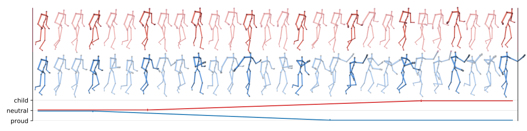
Figure 3: Morphing the style of a human locomotion sequence over time: (red) from neutral to childlike; (blue) from neutral to proud; (bottom) interpolation schedule.

We now turn to real-world applications of the multi-task dynamical system. This section details the first of two such applications: modelling human locomotion. This is a clear example of a sequence family: humans can walk in a variety of different styles depending on their current activity or mood, but for each person there is a unique character present in all these styles. More generally, despite inter-individual differences (see e.g. Lee and Grimson, 2002) there is an intrinsic similarity to all human locomotion. We might therefore expect the majority of such differences to be captured with relatively few degrees of freedom.

To this end, we train an MTDS on motion capture (mocap) data, which is introduced in Section 4.1. The MTDS can help to address several outstanding problems in this context: training dynamical models on limited data, robustness to dataset shift, and style transfer for generative models. We give our experimental results for each of these categories in Section 4.4, with the experimental setup given in Section 4.3. A result of particular interest is that the MTDS allows interpolation or morphing of style over time (see Figure 3), which, to the best of our knowledge, is an entirely novel contribution.

4.1 Data and Pre-Processing

This section provides an introduction to the mocap data that was used (Section 4.1.1), together with the representation constructed for the observations (Section 4.1.2).

4.1.1 Mocap Data

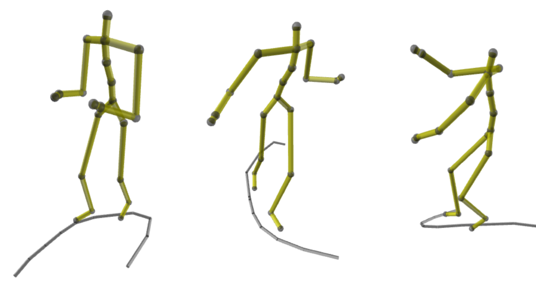
(a)

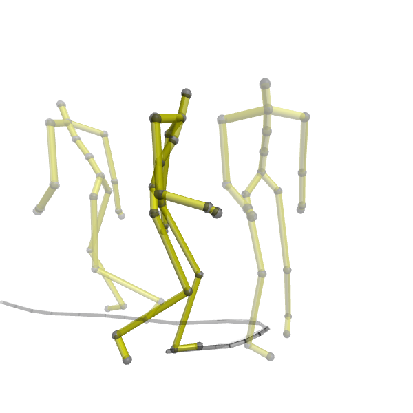
(b)

Figure 4: (a) Example frames from mocap data set, together with $\pm 1$ second ground trajectory shown in grey. (b) Example subsequence where the skeleton rotates in the opposite direction to the corner.

The data are obtained from Mason et al. (2018) which consists of planar walking and running motions in 8 styles recorded with a motion capture (mocap) suit by a single actor. These styles are: ‘angry’, ‘childlike’, ‘depressed’, ‘neutral’, ‘old’, ‘proud’, ‘sexy’, ‘strutting’. The path (or ‘trajectory’) along which the skeleton is walking is provided as an input, in order to avoid modelling the random/unpredictable choices of the actor. See Figure 4 for examples. In this case the sequence family corresponds to the possible walking styles humans exhibit while following a pre-determined path.

The original data is recorded at 120 fps; we downsample to 30 fps as per Martinez et al. (2017); Pavllo et al. (2018). Each style has 3 to 5 individual sequences of varying length, totalling ca. $2000$ frames per style. The data are mapped to a 21-joint skeleton: this is a subset of the CMU skeleton (De la Torre et al., 2009) used by Holden et al. (2016), see Figure 5(a). Unlike Mason et al. (2018), we do not perform any data augmentation such as mirroring. Our interests are primarily in the contribution of the MTDS in modelling style, rather than in producing high fidelity computer graphics. For inputs to the model, we provide the ground trajectory, the gait cycle (a value in $[0,2\pi)$ corresponding to the phase of the leg motion), and a Boolean indicator for the rotational direction while traversing a corner (see Appendix B.1 for further details).

4.1.2 Data Representation

We choose a Lagrangian representation (Figure 5(c)) where the coordinate frame is centered at the root joint of the skeleton (joint 1 in Fig. 5(a), the pelvis), projected onto the ground. The frame is rotated such that the $z$-axis points in the ‘forward’ direction, approximately normal to the plane described by the shoulder blades and pelvis. This is in contrast to the Eulerian frame, which has a fixed position for all $t$ (Figure 5(b)). In the Lagrangian frame, the joint positions are always relative to the root joint, which avoids confusing their motion with the trajectory and rotation of the entire skeleton. The relative joint positions are encoded by position rather than by the angle made with their parent joint. This may result in the model violating bone length constraints, but reduces the sensitivity of internal joints, as discussed for example in §2.1, Pavllo et al. (2018).

Finally, we choose to encode the root joint via its velocity (i.e. via differencing), which allows an animator to more easily amend the trajectory of the model output. We do not represent joints 2 to 21 (relative joint motion) in this way to avoid accumulated errors over time. Our per-frame representation hence consists of the ‘velocity’ $\dot{x},\dot{z},\dot{\omega}$ of the co-ordinate frame, the vertical position of the root joint, and 3-d position of the remaining 20 joints, resulting in $\mathbf{y}_{t}\in R^{64}$. The $\{\mathbf{y}_{t}\}$ are standardized to have zero mean and unit variance per observation channel.

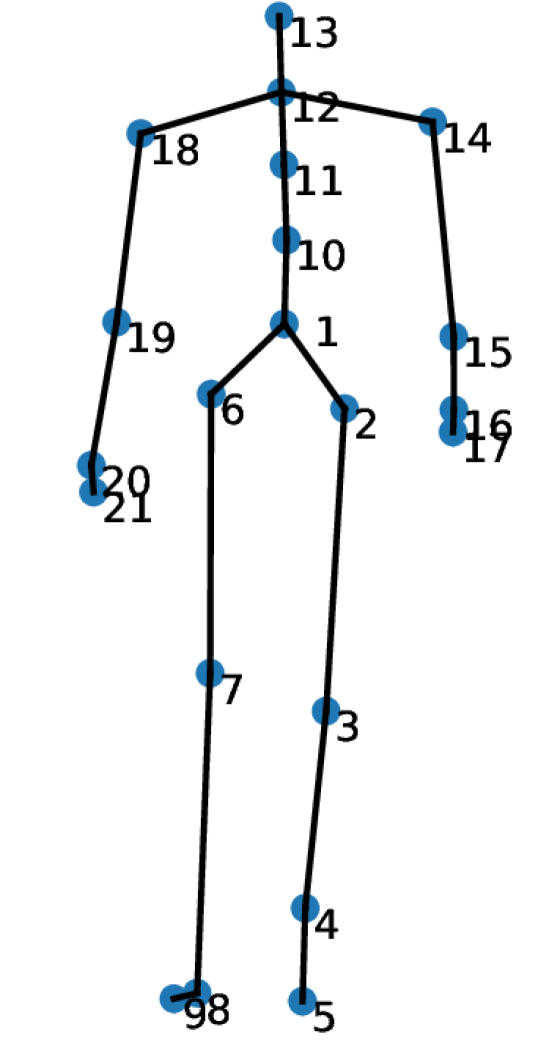
(a)

(b)

(c)

Figure 5: (a) The 21-joint skeleton. (b) Eulerian representation. (c) Lagrangian representation.

4.2 MTDS Model

A natural choice of base model for the MTDS is a RNN (or gated variant such as LSTM or GRU) due to the widespread use of such models in the mocap literature. A graphical model of a multi-task RNN (MT-RNN) is shown in Figure 6(a). Preliminary experiments using MT-RNNs showed strong performance on the training data, but on changing the value of $\mathbf{z}$, predictions either did not change, or became implausible. This appears to be due to some form of information leakage about style (despite substantial efforts to the contrary—see Appendix Section B.1). The RNN was hence performing some of the style inference instead of relying on the latent $\mathbf{z}$. Furthermore, since certain features such as trajectory corner types, or extreme values of speed, or gait frequency are only found within a single style (or group of styles), the response to such unique inputs was only learned for certain values of $\mathbf{z}$.

In order to capture the global input-output relationships across all styles, we propose a 2-layer RNN structure, where the first layer is not multi-task and is able to learn a shared representation across all tasks. The second layer is a MT-RNN which performs specialization to the style using the latent variable $\mathbf{z}$. The separation of responsibility between layers is assisted by three important refinements. The first layer passes information to the second layer via a bottleneck of $\ell$ units, encouraging the first layer to focus on the globally most important features. Secondly, we omit a skip connection from the first layer, which would undermine the bottleneck. Finally, the MT-RNN has a relatively higher learning rate, resulting in a preference to model more variation than the first layer. Since its only inputs are the low-dimensional shared representation of the first layer, $\mathbf{z}$ is forced to explain more of the variance.

(a) XXXX (a) Standard MT-RNN

(b) (b) Proposed MTDS model XXXXXXXX

Figure 6: Graphical model of a standard MT-RNN and the proposed MTDS, for a single style $i$. For clarity, the superscript $i$ is omitted, and the dependence on $\mathbf{z}$ is shown in a different colour.

In detail, our proposed MTDS model is a 2 hidden-layer recurrent model where the first hidden layer is a 1024 unit GRU and the second hidden layer is a 128 unit MT-RNN, followed by a linear decoding layer. Explicitly, omitting index $i$, the model for a style represented by the task variable $\mathbf{z}$ is:

$$[{\bm{\psi}}_{2}(\mathbf{z}),C(\mathbf{z}),\mathbf{d}(\mathbf{z})] =\mathbf{h}_{{\bm{\phi}}}(\mathbf{z}),$$ (12)

$$\mathbf{x}_{1,t} =\textrm{\small GRUCell}_{1024}\left(\mathbf{x}_{1,t\raisebox{-0.45206pt}{\scalebox{0.5}[1.0]{$-$}}1},\,\mathbf{u}_{t};\,\,\,{\bm{\psi}}_{1}\right),$$ (13)

$$\mathbf{x}_{2,t} =\textrm{\small RNNCell}_{128}\left(\mathbf{x}_{2,t\raisebox{-0.45206pt}{\scalebox{0.5}[1.0]{$-$}}1},\,H\mathbf{x}_{1,t\raisebox{-0.45206pt}{\scalebox{0.5}[1.0]{$-$}}1};\,{\bm{\psi}}_{2}(\mathbf{z})\right),$$ (14)

$$\hat{\mathbf{y}}_{t} =C(\mathbf{z})\mathbf{x}_{2,t}+\mathbf{d}(\mathbf{z}),$$ (15)

for $t=1,\ldots,T$; GRUCell, RNNCell are defined in Appendix B.2. See Figure 6b for a graphical model. The parameters which depend on $\mathbf{z}$ are ${\bm{\theta}}=\{{\bm{\psi}}_{2},C,\mathbf{d}\}\in\mathbb{R}^{d}$ and the learnable parameters are thus $\{{\bm{\psi}}_{1},H,{\bm{\phi}}\}$. In our experiments, we use $\ell=24$ units for the bottleneck matrix $H$. The first layer GRU uses 1024 units primarily for qualitative reasons, since it was observed to produce smoother animations than smaller networks. Using a MT-GRU instead of a MT-RNN in the second layer produced worse style transfer; changing the value of $\mathbf{z}$ in this case often made little difference to the style. We have observed in other work that GRUs can more easily perform style inference via use of their gates (see Bird, 2021, §4.5).

The choice of $\mathbf{h}_{{\bm{\phi}}}$ in this instance appears to be relatively unimportant. In practice we used an affine function (i.e. $\mathbf{h}_{{\bm{\phi}}}(\mathbf{z})=W\mathbf{z}+\mathbf{b}$ for $W\in\mathbb{R}^{d\times k}$ and $\mathbf{b}\in\mathbb{R}^{d}$). Preliminary experiments suggested that use of a multi-layer perceptron (MLP) for $\mathbf{h}_{{\bm{\phi}}}$ resulted in similar performance, but initialization was more difficult, and inference of $\mathbf{z}$ was slower.

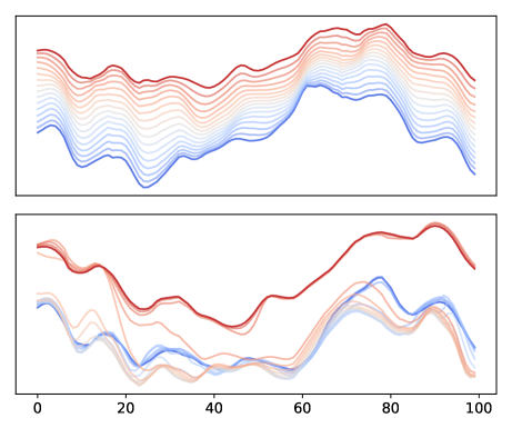
Figure 7: Sequence interpolation for model of joint 11 ($x$ direction) over time $t=1,\ldots,100$ with latent $\mathbf{z}$ varied from ‘strutting’ (blue) to ‘angry’ (red) style. (top) MTDS model; (bottom) MT-Bias model.

In order to ensure smooth variation of the dynamics wrt. $\mathbf{z}$, it proved important to fix the dynamical bias of the MT-RNN layer to a single point estimate (i.e. no dependence on $\mathbf{z}$). Smooth variation of this parameter otherwise resulted in ‘jumps’ when interpolating between sequences styles. A particularly stark example is given in Figure 7 which visualizes various sequence predictions of a given joint while interpolating the latent $\mathbf{z}$ from a ‘strutting’ (blue) to ‘angry’ (red) style. The top figure shows the model output for the MT-RNN model where the bias is fixed wrt. $\mathbf{z}$, the bottom shows the output for the model where only the bias depends on $\mathbf{z}$. We speculate that modulating the bias induces bifurcations in the state space, whereas adapting the transition matrix allows for smooth interpolation. This is consistent with the results of Sussillo and Barak (2013).

4.2.1 Related Work in the Mocap Literature

Generative models for mocap data include those proposed by Wang et al. (2008), Taylor et al. (2010), Holden et al. (2016). Competitive RNN-based approaches are introduced in Fragkiadaki et al. (2015), and Martinez et al. (2017) introduce the idea of sequence-to-sequence or ‘sampling-based’ training (cf. Bengio et al., 2015) in order to avoid predictions converging to a mean pose. We are not aware of any work which learns style-specific representations within the same model, except for Mason et al. (2018) who use residual adapters (and note that no quantitative results are given in their paper); much less of any models which permit style interpolation. The ideas of Tulyakov et al. (2018); Hsieh et al. (2018) (discussed in Sec. 3) may perhaps be applied, but such architectures modulate the style simply via changing the bias or input to the recurrent generation network (similar to Miladinović et al., 2019). While these papers propose additional modifications to the architecture or objective function, we wish to isolate the contribution of our latent $\mathbf{z}$, motivating our decision to consider bias-customized variants as our primary point of comparison.

4.3 Experimental Setup

In order to understand the benefits of the MTDS approach, we consider a number of different experiments which include: performance under limited training data, predictions on novel styles, and style transfer. We provide further details of these in the results section (Section 4.4). In the current section, we discuss the competitor models (Section 4.3.1) and provide an overview of learning and inference (Section 4.3.2).

4.3.1 Benchmark Models

For comparison, we implement a standard 1024-unit GRU pooled over all styles, which serves both as a competitor model (Martinez et al., 2017) and an ablation test. This pooled model can perform some ‘multi-task’-style customization, but in an implicit and black-box manner. Style inference follows the approach of Martinez et al. (2017), where an initial seed sequence $\mathbf{y}_{1\mathrel{\mathop{\mathchar 58\relax}}T_{\textrm{\scriptsize enc}}}$ is provided to the network before prediction. In our experiments we use $T_{\textrm{\scriptsize enc}}=64$ frames. This is essentially a sequence-to-sequence (seq2seq) learning architecture with shared weights between the encoder and decoder.

Secondly, we provide a restricted form of our MTDS model, where only the bias/offset of the RNN is a function of $\mathbf{z}$, providing a comparison to existing work (as discussed above; Section 4.2.1). We denote this simpler approach as the MT-Bias approach in contrast to the full MT approach proposed in this paper. We also provide constant baseline predictions of (i) the training set mean and (ii) the last observed frame of the seed sequence (‘zero-velocity’ prediction).

4.3.2 Learning and Inference

The standard benchmark models were trained by encoding a 64-step seed sequence, and predicting a 64-step forecast without access to the true $\{\mathbf{y}_{t}\}$, in contrast to ‘teacher forcing’. We call this an ‘open-loop’ criterion, as the model receives no feedback during a prediction cycle when training. This forces the model to learn to recover from its mistakes and was first introduced in this context in Martinez et al. (2017). In case the advantage of this is not obvious to the reader, we also provide results using a standard closed-loop criterion (i.e. via teacher forcing) too. For the MT and MT-Bias models, we use a seed sequence to infer the latent $\mathbf{z}$, but not to infer the dynamic state $\mathbf{x}_{0}$ (as in a seq2seq model) to avoid information leakage about the style. Both of these models are learned using the variational procedure described in Section 2.2 and hyperparameters for all models were chosen with respect to a 12.5% validation set. We optimized the posterior distribution of each $\mathbf{z}^{(i)}$ directly for the sake of simplicity, but one can use a recurrent inference network instead such as that proposed in Fabius and van Amersfoort (2015). We report results for a variety of latent dimensions to provide the reader with an intuition of this hyperparameter’s importance. Further details regarding learning can be found in Appendix B.3. The predictive posterior of eq. (9) is used for predictions for MT and MT-Bias models at test time, but due to use of the length-64 seed sequence we found that the posterior was sufficiently concentrated that a MAP estimate of $\mathbf{z}$ performed similarly to our sequential AdaIS method.

4.4 Results

Figure 8: $k=8$ mean embedding of each sequence segment, visualized via t-SNE, coloured by its (unseen) task label.

Figure 8 shows a t-SNE plot (Van der Maaten and Hinton, 2008) of the $k=8$ mean embedding of $\mathbf{z}$ for each of the 64-frame segments in the data set, coloured by the true style label. (We remind the reader that this label is unavailable during training.) Our MTDS model can successfully disambiguate the styles without supervision, and in fact provides a more fine-grained representation than the original labels. Many walking styles have at least two sub-styles (e.g. ‘childlike’ comprises both skipping and juggling motions). This visualization suggests that our MTDS model can indeed learn a useful manifold over sequence styles; further investigation in Section 4.4.4 validates the intermediate points on this manifold, and demonstrates the potential of style interpolation.

This granular description of sequence style, and customization of predictions is unavailable from any of our competitor models. In the case of standard GRUs, style customization is occurring, but it is entangled in the various hidden units, and unavailable to an end user. Moreover, it cannot be controlled should a different style be desired. MT-Bias models appear to achieve a poorer latent representation than the full MT approach (see Appendix B.4.1 where the MT-Bias shows substantial conflation of styles). This results in significantly less control over style than our MTDS model, as is demonstrated in the style transfer experiments in Section 4.4.3, as well as poorer inter-style interpolation (as e.g. in Figure 7).

To demonstrate the benefit of the MTDS approach quantitatively, we provide results from three experiments, concerning: data efficiency (Sec. 4.4.1), performance on unseen walking styles (Sec. 4.4.2), and style transfer (Sec. 4.4.3). We conclude in Section 4.5.

4.4.1 Data Efficiency

		MSE
		Training set size
Model		3%	7%	13%	27%	53%	97%
Training mean		0.76	0.76	0.72	0.73	0.73	0.73
Zero-velocity		1.23	1.23	1.23	1.23	1.23	1.23
STL GRU (open loop)		1.11	0.88	0.40	0.33	0.18	0.18
Pooled GRU (closed loop)		0.79	0.61	0.82	0.87	0.76	1.21
Pooled GRU (open loop)		0.69	0.52	0.36	0.29	0.16	0.16
MT Bias ($k=3$)		0.93	0.44	0.30	0.21	0.14	0.16
MT Bias ($k=5$)		0.98	0.44	0.30	0.20	0.14	0.16
MT Bias ($k=7$)		0.94	0.49	0.30	0.21	0.15	0.16
MTDS ($k=3$)		0.62	0.34	0.35	0.21	0.21	0.19
MTDS ($k=5$)		0.53	0.29	0.22	0.19	0.15	0.16
MTDS ($k=7$)		0.51	0.27	0.24	0.20	0.16	0.18

Table 1: Experiment 1 (data efficiency): MSE for length-64 predictions where training set size is expressed as a fraction of the original data set. The best performances for each training set size (up to $\alpha=0.05$ significance—see text) are shown in bold.

We test the conventional advantage of MTL by considering reduced subsets of the original data set. We perform six experiments which use between $2^{8}$ to $2^{13}$ frames per style (logarithmically spaced) for training, with sampling stratified carefully across major variations of all styles. A ‘single-task’ 1024-unit GRU benchmark is also included for comparison, which is trained and tested on a single style. In all cases, the test performance (MSE) is calculated from 4 held-out sequences from each style (64 frames each), and averaged over all styles.

The results for the six data set sizes are shown in Table 1. Results in each column are compared to the best performing model using a paired $t$-test; the results which have comparable performance to the best model (i.e. are not significantly different at an $\alpha=0.05$ level) for the held out sequences are shown in bold. The open-loop GRU (Martinez et al., 2017) performs far better than the standard closed-loop variant, and we will omit the latter from further discussion. The results show strong performances for the MTDS approach, which tends to perform best for $k>3$ (results for $k=5$ and $k=7$ are not significantly different). For small data sets (< 50% of the data set), we observe advantages from all multi-task models (including the Pooled GRU) over a STL approach. However, the MTDS demonstrates far superior performance than the other MT approaches for smaller data sets; achieving a MSE of 0.27 after only 7% of the data set. The MT-Bias model requires more than twice this amount of data to obtain the same performance, and the Pooled GRU requires more than four times this amount. These results are plotted graphically in Figure 9(a). For data set sizes up to (and including) 13% of the original, the MTDS is equal or better across all styles and data set sizes, except for the {‘angry’, ‘sexy’} styles for the smallest data set (data not shown).

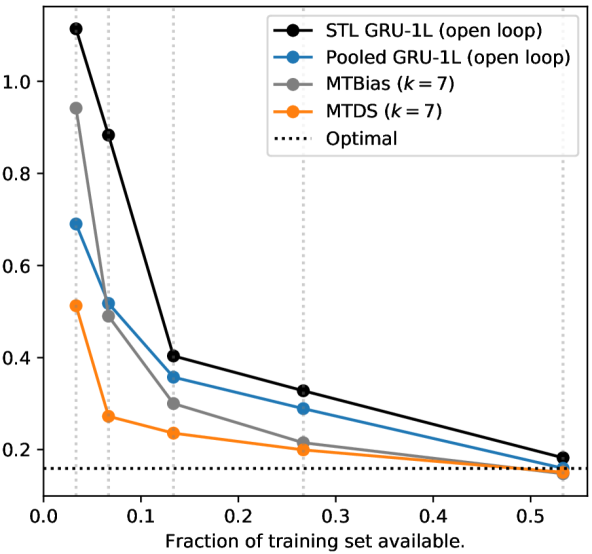
(a)

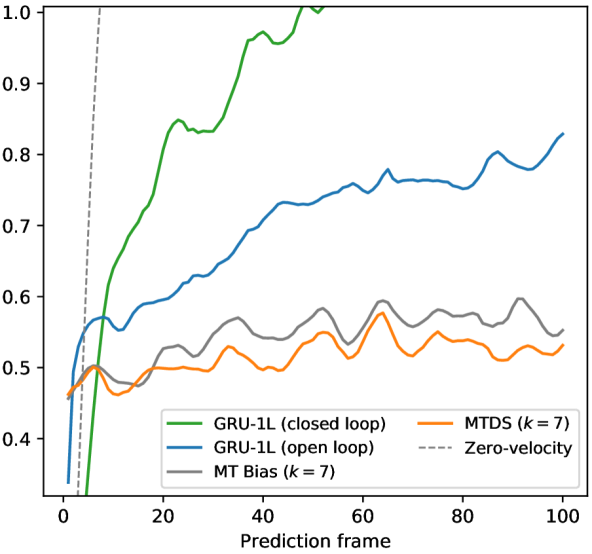
(b)

Figure 9: (a) Experiment 1 (data efficiency): out-of-sample MSE by % of training set seen. The performance achieved by the GRU models for the entire training set is shown as the ‘Optimal’ dashed line. (b) Experiment 2 (novel test data): MSE performance (avg over folds).

4.4.2 Novel Test Data

Our second experiment investigates how well the MTDS can generalize to novel sequence styles. This is similar to a domain adaptation or zero-shot learning task. We consider a leave-one-out (LOO) procedure with eight folds, where each fold has a training set comprising 7 styles, and a test set comprising the held-out style. We consider the deterioration of predictive MSE over a large time window ($\tau\leq 200$ frames, ca. 7 seconds). It can be relatively easy to predict $\tau$-steps ahead for $\tau\leq 10$ (see Martinez et al., 2017) even for novel sequences, but the error usually deteriorates with increasing $\tau$. Our results report the predictive MSE for each $\tau$ averaged over the 8 folds, and over 32 different starting locations within each fold. The competitor models are as above (excluding the STL model), but we also include a 2-layer GRU (with 1024 units in each layer) as the training set is larger than in the previous experiment and can reliably learn such a model.

A summary of results is shown in Figure 9(b), where the axes are truncated for clarity. The standard Pooled GRUs work well for small values of $\tau$ but degrade very quickly. The closed-loop variants perform the best for $\tau\leq 5$ but degrade even more rapidly than the open-loop approach. The deteriorating results for these models are consistent with the inputs moving the state into an area where the dynamics have not been trained. In contrast, the MTDS and MT-Bias models find a better customization which evidences very little worsening over the predictive interval. Importantly, these models are able to ‘remember’ their customization over long intervals via the latent $\mathbf{z}$. The $k=7$ MTDS shows equal or better performance to the pooled GRU on all styles for $\tau\geq 10$, and its initial performance may perhaps be improved via interpolation from the seed sequence given the performance of the ‘zero-velocity’ baseline for $\tau\leq 5$. The results of the 2-layer competitors are shown in Table 2, but they achieve similar performance to the 1-layer models on aggregate (a similar result is suggested in Martinez et al., 2017).

		MSE
Model		$\tau=5$	$\tau=10$	$\tau=20$	$\tau=50$	$\tau=100$	$\tau=200$
Training mean		1.04	1.04	1.05	1.04	1.06	1.07
Zero-velocity		0.69	1.20	1.37	1.21	1.35	1.48
Pooled 1-layer GRU (closed loop)		0.35	0.64	0.81	1.00	1.45	7.28
Pooled 2-layer GRU (closed loop)		0.34	0.61	0.79	0.97	1.41	6.34
Pooled 1-layer GRU (open loop)		0.56	0.56	0.60	0.73	0.83	0.92
Pooled 2-layer GRU (open loop)		0.53	0.55	0.59	0.73	0.85	0.94
MT Bias ($k=3$)		0.60	0.60	0.58	0.59	0.64	0.63
MT Bias ($k=7$)		0.50	0.48	0.53	0.57	0.55	0.63
MTDS ($k=3$)		0.61	0.62	0.59	0.61	0.63	0.63
MTDS ($k=7$)		0.49	0.46	0.50	0.54	0.53	0.61

Table 2: Experiment 2 (novel test data): average predictive MSE at $\tau=5,10,20,50,100,200$. The best performing model(s) (up to $\alpha=0.05$ significance) for each $t$ is highlighted in bold.

These experiments demonstrate that it can be crucial to retain control over the task inference for novel data, rather than delegating it to a black-box procedure; the implicit inference of standard GRU networks can perform very poorly when presented with unexpected inputs. For this experiment, while the full MTDS consistently outperforms the MT-Bias approach, the difference is not large. In practice, perhaps either could be used. We note that all models struggle to capture the arm movements of the unseen styles since these are often entirely novel. Customization to the legs and trunk is easier since less extrapolation is required (see animation videos linked in Section 4.4.4).

4.4.3 Style Transfer

Finally, we investigate how much user control is available via the latent code, $\mathbf{z}$. We can hold the input trajectory $\{\mathbf{u}_{t}\}$ constant, and vary the latent $\mathbf{z}$ from its inferred position. In theory, this should result in style transfer: the same trajectory of locomotion but performed in a different style. This is unavailable from any existing GRU approaches (see related work), and hence in this section we can only compare the full MTDS with the restricted MT-Bias model. For each pair of styles $(s_{1},s_{2})$ we investigate style transfer from a source sequence of style $s_{1}$ to a target style $s_{2}$. Due to the within-style variation, we use four different source sequences for each pair $(s_{1},s_{2})$. We learn the embedding using a $k=8$ model, and choose a single latent value $\mathbf{z}^{(s_{2})}$ for each of the eight target styles $s_{2}=1,\ldots,8$ to perform the style transfer; see Appendix B.4.2 for more details. Evaluation is performed via use of a classifier, for which we use a 512-unit GRU to encode the sequence followed by a 300-unit hidden layer MLP with multinomial emissions. The classifier is trained on the complete data using the (previously unused) labels from Mason et al. (2018). Qualitative results are available via the videos linked in Section 4.4.4, and further experimental details are given in Appendix B.4.2.

Target	Angry	Child	Depr.	Neut.	Old	Proud	Sexy	Strut
MT Bias	0.78	0.59	0.65	0.79	0.55	0.71	0.55	0.71
MTDS	0.86	0.95	0.81	0.93	0.86	0.82	0.90	0.92

Table 3: Experiment 3 (style transfer): classifier probability of target style averaged over all input styles.

The results are summarized in Table 3, which provides the average ‘probability’ assigned by the classifier for each target style $s_{2}$, averaged over all the input sequences where the source $s_{1}\neq s_{2}$. (The best performing model for each style is highlighted in bold.) Successful style transfer should result in the classifier assigning a high probability to the target style. The results suggest that the style can generally be well controlled by $\mathbf{z}$ in the case of the full MTDS, but the MT-Bias model exhibits reduced control for some (source, target) pairs. Style transfer appears to be easier between more similar styles; the lowest scores tend to be for transfer from the ‘childlike’ and ‘angry’ styles (which have unusually fast trajectories) or the ‘old’ style (which has unusually slow ones). Appendix B.4.2 provides a more detailed comparison of this performance.

These results demonstrate that an MTDS approach can provide end-user control of task-level attributes, in this case resulting in style transfer. We have also seen that our full MT parameterization provides far greater control than the limited MT-Bias approach. Some insight is available from the respective latent representations (Appendix B.4.1), for which the MT-Bias model has apparently conflated a variety of styles. In this case, such styles can only be disambiguated via the inputs, and changing the latent $\mathbf{z}$ alone may result in unrecognizable changes. Further improvements to the MTDS may be possible via use of domain knowledge or adversarial objectives; we leave this to future work.

4.4.4 Qualitative Results

Finally, we discuss the qualitative results of our MTDS model, making use of the latent representation (as in Figure 8, page 8) and animations of the predictions.

The latent representation of the MTDS appears sensible; similar motions are located close together, and differing ones are further apart. For instance, the neighboring ‘old’ and ‘depressed’ styles in Figure 8 both involve leaning over, and the neighboring ‘childlike’ and ‘sexy’ clusters both comprise ‘skipping’-type motions. As such, the learned embeddings appear to capture more information than the original labels. Smooth interpolation between styles is also available from the full MTDS model as suggested by Figure 3 (page 3), and Figure 7 (top, page 7); this can be verified in the animations linked below. Interpolation of the style manifold of the MT-Bias model tends to result in ‘jumps’, as suggested by Figure 7 (bottom).

The animations for all experiments have been collected into a project webpage. They form a crucial part of the model evaluation, which cannot be adequately summarized in static figures. These animations include:

1. In-sample predictions: demonstrating the best possible performance of the models.

2. MTL examples from Section 4.4.1 comparing the quality of animations and fit to the ground truth for two limited training set sizes (6.7% and 13.3% of the full data).

3. Novel test examples from Section 4.4.2 showing the adaptions obtained by each model to novel sequences.

4. Style morphing. This animation demonstrates the effect of interpolating $\mathbf{z}$ over time by morphing between all eight styles, which goes beyond the style transfer of Section 4.4.3.

4.5 Conclusion

We have shown that the MTDS framework can be applied to RNN-type models and can capture the inter-sequence differences of a training set ${\mathcal{D}}$ using the latent variable $\mathbf{z}$. This is not limited to simple low-dimensional sequences, but can be applied to complex sequences with highly nonlinear relationships, such as mocap data. Our experiments have suggested a number of advantages over existing approaches. Firstly, the MTDS can result in substantial improvements in performance in small data settings. Secondly, the same model can avoid performance deterioration under dataset shift, and thirdly, be used to perform highly effective style transfer. Finally, the resulting sequence family admits interpolation between its members, which for this application produces smooth morphing between walking styles.

5 Application to Drug Response Data

Our second application of the multi-task dynamical system is in the medical domain. In this context (unlike many high-profile applications of machine learning) sample sizes are small, and consequences of mistakes can be severe. For this reason, models tend to be simple, inflexible and predict average effects. Personalization of these models is often thought to require larger samples and more covariates (e.g. genomic and proteomic data), and thus the necessary data sets may be unavailable for many years to come, and carry increased requirements for secure infrastructure and privacy protection. Our notion of a sequence family, modelled by a multi-task dynamical system (MTDS), allows us to take a step towards personalization without this additional data.

In this section, we consider the example of predicting patient response to the anaesthetic agent propofol. We learn a family of possible responses, using a MTDS, and provide an increasingly personalized prediction as more observations are seen. Our goal is not to provide the best possible model, but to show how the MTDS can personalize the existing model that is in use by current practitioners. We may hence improve predictions while maintaining trust. If an alternative model becomes acceptable to clinicians in future, then the MTDS can equally be applied to this too.

This section is structured as follows: Section 5.1 introduces the modelling background, Section 5.2 describes our proposed base model and the MTDS variant. Section 5.3 introduces the experiments, and the results are provided in Section 5.4. We conclude in Section 5.5.

5.1 Background

In this section, we introduce the modelling task (Section 5.1.1), discuss existing approaches (PK/PD models, Section 5.1.2), and provide the necessary background of our target model (Section 5.1.3).

5.1.1 Introduction

In order to sedate a patient, an anaesthetist initially targets a certain blood concentration of an anaesthetic agent. In the case of propofol, this may be between 0.5 - 5.0 $\mu$g/ml. The drug is administered via use of an intravenous infusion pump, which uses an internal model to provide the desired concentration. The response of the patient is quantified via vital signs, providing an important feedback loop to anaesthetists; in our case the vital signs are systolic and diastolic blood pressure and BIS, a measure of consciousness.

The patient response to the drug infusion depends on their physiology, resulting in substantial inter-patient variation. Some examples of modelled responses to the same infusion sequence are shown in Figure 10(a) for systolic blood pressure; real data exhibit similar inter-patient differences. The initial dosage targets a BIS value in the range 40-60, but the vital signs must be monitored on a continual basis to ensure the patient stays within the therapeutic window. This task is made substantially harder due to the lag between dose and response. Further complications are introduced in practice (e.g. due to surgical stimuli or multiple drugs); we limit the scope of this work to predict the response to a single drug (propofol) in a stationary environment. This is an important first step towards a control system for steady state anaesthetic maintenance, with the potential to free up considerable time from practicing anaesthetists.

5.1.2 PK/PD Models

Drug response is typically modelled via pharmacokinetic/pharmacodynamic (PK/PD) models. See Bailey and Haddad (2005) for an introduction. The PK component models the distribution of drug concentration throughout the body. There is substantial existing work for personalizing PK models (important examples include Marsh et al. 1991; Schnider et al. 1998; White et al. 2008; Eleveld et al. 2018). Various studies (see e.g. Masui et al., 2010; Glen and White, 2014; Hüppe et al., 2019) have compared the predictive performance of propofol PK models currently used in clinical practice. These studies have confirmed a degree of bias and inaccuracy of the models but overall their performance is considered by most clinicians to be adequate for clinical use (at least within the populations in which they were developed).

A PD model maps the drug distribution estimated by the PK model to the physiological effect. In practice, it is difficult to provide analytic models of PD processes, and most proposals instead take an empirical approach (Bailey and Haddad, 2005). However, despite the relatively simple models proposed, there is comparatively little work on their personalization. Many commercially available implementations of the Marsh and Schnider models use fixed population-level parameters, but it is widely accepted by practicing anaesthetists that there exists a significant amount of inter-individual variability in PD response to propofol, a point recently demonstrated in Van Hese et al. (2020). Eleveld et al. (2018) adjust the PD parameters based on age, but the available improvements are relatively small. Since there is more scope to improve this component, we focus our efforts on providing a personalized PD model, and use the PK model of White et al. (2008) as-is.

(a)

(b)

Figure 10: (a) Differing systolic blood pressure responses across patients to a given drug infusion shown in the bottom panel. The responses follow individual PD models trained offline. (b) A standard PK/PD model. The effect compartment $C_{e}$ of the PD model attaches to the central compartment, $C_{1}$ of the PK model. The concentration in $C_{e}$ is assumed to be directly related to the pharmacodynamic effect, $\mathbf{y}$, e.g. BPsys as in the opposite figure.

5.1.3 PD Models

Most PD models propose that the physiological effect can be determined directly (up to random noise) from the drug concentration at some effect site ($C_{e}$). This is a notional physiological site which contains the receptors bound by the drug compound of interest. The concentration of the drug at $C_{e}$ is affected by the concentration in the blood plasma, modelled in the PK model as the central compartment, $C_{1}$. We will denote the concentration of the two sites as $x(t)$ and $c_{1}(t)$ respectively. A lag between these two concentrations is usually observed, and may be caused by multiple factors including distribution, receptor binding time, and the effects of intermediate substances. For more details see e.g.  Holford (2018).

A standard choice in the PD literature is to model the effect site concentration $x(t)$ by the following differential equation:

$$\frac{\operatorname{d\!}x}{\operatorname{d\!}t}=k_{1e}c_{1}(t)-k_{e0}x(t),$$ (16)

where the rate of in-flow to the effect site is denoted $k_{1e}$ and the elimination rate is denoted $k_{e0}$. We assume that the central compartment concentration $c_{1}(t)$ is available (via application of a PK model to the raw drug infusion sequence $\omega(t)$). A schematic is shown in Figure 10(b). Where multiple effects are observed simultaneously (e.g. BPsys, BPdia, BIS), it is common to use one effect site per observation channel, resulting in effect site concentrations $x_{j}(t)$ for $j=1,\ldots,n_{y}$. The relationship of $\mathbf{x}(t)$ to the observations $\mathbf{y}(t)$ is usually modelled by some nonlinear transformation $\mathchoice{g_{\raisebox{-0.95pt}{\scalebox{0.7}{$\displaystyle{\bm{\eta}}$}}}}{g_{\raisebox{-0.95pt}{\scalebox{0.7}{$\textstyle{\bm{\eta}}$}}}}{g_{\raisebox{-0.95pt}{\scalebox{0.7}{$\scriptstyle{\bm{\eta}}$}}}}{g_{\raisebox{-0.95pt}{\scalebox{0.7}{$\scriptscriptstyle{\bm{\eta}}$}}}}$ plus white (Gaussian) noise, i.e. for a given time $t$,

$$y_{j}(t)\,\sim\,\mathcal{N}\left(\mathchoice{g_{\raisebox{-1.3pt}{\scalebox{0.7}{$\displaystyle{\bm{\eta}}_{j}$}}}}{g_{\raisebox{-1.3pt}{\scalebox{0.7}{$\textstyle{\bm{\eta}}_{j}$}}}}{g_{\raisebox{-1.3pt}{\scalebox{0.7}{$\scriptstyle{\bm{\eta}}_{j}$}}}}{g_{\raisebox{-1.3pt}{\scalebox{0.7}{$\scriptscriptstyle{\bm{\eta}}_{j}$}}}}(x_{j}(t)),\mkern 4.0mu\nu_{j}^{-1}\right),$$ (17)

for $j=1,\ldots,n_{y}$ with parameters ${\bm{\eta}},\bm{\nu}$. Most common choices of $\mathchoice{g_{\raisebox{-0.95pt}{\scalebox{0.7}{$\displaystyle{\bm{\eta}}$}}}}{g_{\raisebox{-0.95pt}{\scalebox{0.7}{$\textstyle{\bm{\eta}}$}}}}{g_{\raisebox{-0.95pt}{\scalebox{0.7}{$\scriptstyle{\bm{\eta}}$}}}}{g_{\raisebox{-0.95pt}{\scalebox{0.7}{$\scriptscriptstyle{\bm{\eta}}$}}}}(\cdot)$ are sigmoidal in nature and include the Hill function (Wagner, 1968) and the generalized logistic sigmoid (Georgatzis et al., 2016).

5.2 Proposed Model

In this section, we consider learning a sequence family of PD responses using an MTDS, conditioned on a propofol infusion sequence. At test time we can choose the most probable future response from the family by comparison to the patient’s current observations. The parameterization of the base PD model is described in Section 5.2.1 followed by the MTDS version in Section 5.2.2 which enables online personalization. We compare this to related work in 5.2.3.

5.2.1 Base PD Model

Our proposed base model is a relaxation of the PD model described above in discrete time. We assume access to the PK model prediction applied to each drug infusion sequence. Specifically, let the inputs $\{u_{t}\}$ be the modelled central compartment concentration discretized on the unit grid $t=1,\ldots,T$, using the parameters of White et al. (2008). Denoting the effect site concentration at time $t$ as $x_{t}$, eq. (16) may be discretized as:

$$x_{t} =\beta_{1}x_{t-1}+\beta_{2}u_{t-1},$$ (18)

for some $\beta_{1}$, $\beta_{2}$, with no loss of generality if $c_{1}(t)$ is constant in each interval $(t-1,t]$. These coefficients are related to the rate constants as:

$$\beta_{1}\, =\,e^{-k_{e0}}\qquad \Rightarrow\beta_{1}\,\in\,(0,1)$$

$$\beta_{2}\, =\,\frac{k_{1e}}{k_{e0}}\left(1-e^{-k_{e0}}\right)\qquad \Rightarrow\beta_{2}\,>\,0,$$

since the rate constants are positive. We derive these relationships via use of Laplace transforms and the convolution theorem (see Appendix C.2 for further details). Since $\beta_{1}\in(0,1)$, the ARX(1) process in eq. (18) is stable and non-oscillating.

The nonlinear emission is modelled via a function $\mathchoice{g_{\raisebox{-0.95pt}{\scalebox{0.7}{$\displaystyle{\bm{\eta}}$}}}}{g_{\raisebox{-0.95pt}{\scalebox{0.7}{$\textstyle{\bm{\eta}}$}}}}{g_{\raisebox{-0.95pt}{\scalebox{0.7}{$\scriptstyle{\bm{\eta}}$}}}}{g_{\raisebox{-0.95pt}{\scalebox{0.7}{$\scriptscriptstyle{\bm{\eta}}$}}}}(\cdot)$ with parameter vector ${\bm{\eta}}$. We have found the choices in previous work (generalized sigmoid, Hill function) to be numerically unstable for gradient-based optimization or insufficiently flexible. Instead we use a basis of logistic sigmoid ($\sigma$) functions and express:

$$\mathchoice{g_{\raisebox{-0.95pt}{\scalebox{0.7}{$\displaystyle{\bm{\eta}}$}}}}{g_{\raisebox{-0.95pt}{\scalebox{0.7}{$\textstyle{\bm{\eta}}$}}}}{g_{\raisebox{-0.95pt}{\scalebox{0.7}{$\scriptstyle{\bm{\eta}}$}}}}{g_{\raisebox{-0.95pt}{\scalebox{0.7}{$\scriptscriptstyle{\bm{\eta}}$}}}}(x)\,=\,\sum_{r=1}^{L}\eta_{r}\,\sigma(\,a_{r}(x-b_{r})),$$ (19)

with constants $a_{r}<0$ and coefficients $\eta_{r}\geq 0$ for all $r$. These constraints enforce the desired monotonicity that as concentration increases, the observations (blood pressure etc.) are non-increasing. We fitted an 8-dimensional basis with pre-selected constants $\{a_{r},b_{r}\}_{r=1}^{8}$ chosen by optimising the fit to the learned generalized sigmoid functions used by Georgatzis et al. (2016).

To complete the model, we introduce additional parameters $\bm{\beta}_{3}$ and $\bm{\alpha}$ which provide personalized offsets to the values of the effect site dynamics and the emission respectively. These are degrees of freedom one might expect in a dynamical system, but are not present in the usual PD formulation. The full model for a given patient can be written with $\mathbf{x}_{t}\in\mathbb{R}^{n_{x}}$ and $\mathbf{y}_{t}\in\mathbb{R}^{n_{y}}$ as:

$$\mathbf{x}_{t}\, =\,{\bm{\beta}}_{1}\odot\mathbf{x}_{t-1}\,+\,{\bm{\beta}}_{2}u_{t}$$ (20a)

$$y_{tj}\, =\,\mathchoice{g_{\raisebox{-1.3pt}{\scalebox{0.7}{$\displaystyle{\bm{\eta}}_{j}$}}}}{g_{\raisebox{-1.3pt}{\scalebox{0.7}{$\textstyle{\bm{\eta}}_{j}$}}}}{g_{\raisebox{-1.3pt}{\scalebox{0.7}{$\scriptstyle{\bm{\eta}}_{j}$}}}}{g_{\raisebox{-1.3pt}{\scalebox{0.7}{$\scriptscriptstyle{\bm{\eta}}_{j}$}}}}(x_{tj}+\beta_{3j})\,+\,\alpha_{j}\,+\,\epsilon_{tj},$$ (20b)

$\epsilon_{tj}\sim\mathcal{N}\left(0,\,\nu_{j}^{-1}\right)$ for $j=1,\ldots,n_{y}$ and $t=1,\ldots,T$. Here $\bm{\beta}_{j}\in\mathbb{R}^{n_{y}},j=1,\ldots,3$, with each dimension corresponding to the parameters of each channel’s dynamics, $\bm{\eta}_{j}\in\mathbb{R}^{L},j=1,\ldots,n_{y}$ are the per-channel nonlinear coefficients (see eq. 19) and $\odot$ denotes elementwise multiplication.

This results in a nonlinear deterministic-state dynamical system where each dimension is independent. A stochastic state might be considered as an extension to the standard PD approach, but preliminary investigation showed superior predictions with the deterministic approach. The parameters of the model are $\bm{\nu}$ and ${\bm{\theta}}=\{\bm{\alpha},$ $\bm{\beta}_{1},\bm{\beta}_{2},\bm{\beta}_{3},$ ${\bm{\eta}}_{1},\ldots,{\bm{\eta}}_{n_{y}}\}\in\mathbb{R}^{d}$, $d=36$, while $\mathbf{a},\mathbf{b}$ are constants. In principle, $\bm{\alpha}$ may be estimated prior to anaesthetic induction since it relates to pre-infusion patient-specific vitals levels.

5.2.2 MTDS Model

We now discuss a version of this PD model which can achieve increasing personalization over time. Unlike the MT-RNN in Section 4, it is not entirely impractical to place an uninformative prior over ${\bm{\theta}}$ and perform Bayesian inference online. But this ‘single task’ (ST) approach fails to take advantage of the inductive bias from the training data, resulting in poor performance for patients with limited data, and poorly conditioned and expensive inference. An MTDS approach avoids these limitations; we describe its application below.

We assume that each patient $i$ can be described by the above PD model with parameter ${\bm{\theta}}^{(i)}$. The parameters for patient $i$ (denoted with the associated superscript) will be modelled by use of a latent code $\mathbf{z}^{(i)}\in\mathbb{R}^{k}$ with prior $\mathbf{z}^{(i)}\,\sim\,\mathcal{N}\left(0,I_{k}\right)$ which relates to the parameters as:

$${\bm{\theta}}^{(i)}\,=\,[\bm{\alpha}^{(i)},{\bm{\beta}}_{1}^{(i)},{\bm{\beta}}_{2}^{(i)}, \,{\bm{\beta}}_{3}^{(i)},{\bm{\eta}}_{1}^{(i)},\ldots,{\bm{\eta}}_{n_{y}}^{(i)}]\,=\,\mathbf{h}_{{\bm{\phi}}}(\mathbf{z}^{(i)}).$$ (21)

See Figure 11(a) for a graphical model. Here we choose $\mathbf{h}_{{\bm{\phi}}}(\mathbf{z})\,=\,\mathbf{f}(\Phi\mkern 1.5mu\mathbf{z}+\mathbf{c})$ for some ‘loading matrix’ $\Phi$, offset $\mathbf{c}$ and elementwise transformation function $\mathbf{f}$ (see below). This construction extends the basic PD model in eq. (20) to a family of PD models, where each patient has a personalized parameter vector ${\bm{\theta}}^{(i)}$. The improvements over the ST approach are facilitated by the rank-$k$ $\Phi$, and the ‘default’ parameter ${\bm{\theta}}^{(0)}\vcentcolon=\mathbb{E}_{p(\mathbf{z})}[\mathbf{h}_{{\bm{\phi}}}(\mathbf{z})]$ learned from the training data. We call this an ‘MTPD’ model.

The function $\mathbf{f}$ consists of elementwise univariate transformations which ensure that each parameter satisfies the required constraints. For example, the unit interval constraints for ${\bm{\beta}}_{1}^{(i)}$ is enforced via a logistic sigmoid, and the non-negativity constraints for ${\bm{\beta}}_{2}^{(i)}$ by $\text{softplus}(x)=\log(1+e^{x})$ etc. If parameters are unconstrained, no nonlinearity is applied. The use of an (elementwise constrained) affine $\mathbf{h}_{{\bm{\phi}}}$ can result in an interpretable latent code for clinical practice; the meaning of each element of $\mathbf{z}$ can easily be obtained via inspection of the matrix $\Phi\in\mathbb{R}^{d\times k}$.

We have formulated this model for an unknown $\mathbf{z}$ which is inferred over time. However, some information may be gleaned from covariates $\bm{\zeta}$ such as age, height, weight etc. To the extent that these covariates ‘describe’ the differences between patient responses, we can set $\mathbf{z}\leftarrow\bm{\zeta}$ which we call a task-descriptor approach. In this case, test time inference is not required, but the model cannot adapt to the response. A hybrid approach is also possible, which performs inference only on a subset of the dimensions of $\mathbf{z}$.

(a)

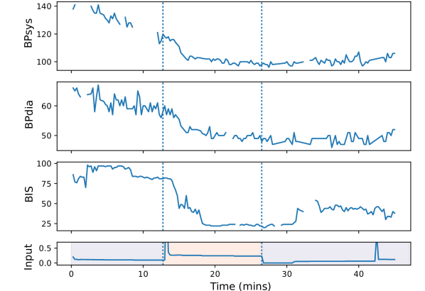
(b)

Figure 11: (a) MT PD model for a single patient; the superscript $i$ is omitted for clarity. (b) Vital signs ($\mathbf{y}_{t}$) and drug infusion ($u_{t}$) for an example patient.

5.2.3 Related Work

We pause here to briefly review related work in the machine learning literature concerning personalized treatment modelling. Deep learning methods are not considered, due to the small sample sizes encountered in clinical trials. Georgatzis et al. (2016) demonstrate that relaxing the PK/PD model class to a general state space model can result in improved model fit and in-sample prediction, but such models cannot be applied to new patients at test time. Multi-task GPs (MTGPs) have been used for condition monitoring, for example in Dürichen et al. (2015), but for gaining strength over multiple observation channels. The approach cannot easily gain strength over different patients (see MTGP discussion in Section 3) and further, cannot integrate control inputs. Alaa et al. (2018) permit gaining strength over patients via use of a mixture of GPs. But in their work, personalization is achieved via use of covariates, restricted to a fixed set of subtypes, and is still unable to integrate control inputs.

Schulam and Saria (2015) propose a form of generalized linear mixed effects model, which assumes an additive decomposition of population, individual and (GP-based) noise components. Further extensions are proposed in Xu et al. (2016); Futoma et al. (2016), but these approaches only adjust linear coefficients, and cannot customize dynamical parameters. These approaches are extended further by Soleimani et al. (2017); Cheng et al. (2020), who include first order ODEs of control inputs. Nevertheless, these still relate additively to the observations (exploiting the linearity of GPs); extensions to nonlinear dynamical systems (e.g. PK/PD models) are not straight-forward. Furthermore, no methods for online inference are presented, and no multi-task ideas are used; adaptivity is restricted to simple mixed effects.

5.3 Experimental Setup

This section describes the experimental setup for the evaluation of our model. Section 5.3.1 describes the data, Section 5.3.2 describes the form of evaluation, and the details of the models under comparison are given in Section 5.3.3 - Section 5.3.4.

5.3.1 Data

The data were obtained from an anaesthesia study carried out at the Golden Jubilee National Hospital in Glasgow, Scotland, as described in Georgatzis et al. (2016). These consist of $N=40$ time series of Caucasian patients; the median length is 36 minutes (range approx. 27 - 50 mins) and the data are subsampled to 15-second intervals. Each patient was assigned to one of two pre-operative infusion schedules of propofol following a high-low-high or low-high-low sequence (see Appendix C.1). Each patient has additional covariates of age, gender, height, weight (and body mass index). The observations $\mathbf{y}_{t}$ at each time $t$ have $n_{y}=3$ channels comprising systolic and diastolic blood pressure (BPsys, BPdia) and BIS, however 13 patients have no BIS channel, which is considered as missing data. An example time series is shown in Figure 11(b): the observations $\{\mathbf{y}_{t}\}$ are shown in the top panels, and the raw drug infusion input at the bottom. The infusion schedule is indicated via the vertical dotted lines with the middle section targeting a higher propofol concentration. One can observe many of the discussed features here including lagged and nonlinear responses. The missing values are due to sensor dropouts and other noise which was removed with clinical supervision.

5.3.2 Evaluation

We evaluate predictions from our MTPD model by Root Mean Squared Error (RMSE) over 20- and 40-step ahead windows (a clinically relevant interval of 5 or 10 mins). The performance is reported at both 12 minutes and 24 minutes to understand if the predictions are improving over time. We follow a leave-one-out (LOO) procedure due to the relatively small number of patients (in machine learning terms); for each of 40 folds, a model is learned on 39 patients and tested on the held-out patient, and the results are averaged. During training, the RMSE is weighted such that each patient has an equal contribution to the objective despite differing sequence lengths, to avoid a bias towards patients with longer sequences.

Name	Parameters	Adapt-  ive $\bm{\alpha}$	Details
Pooled	${\bm{\theta}}={\bm{\theta}}_{0}$	✗	One-size-fits-all model.
Pooled-$\alpha$	${\bm{\theta}}={\bm{\theta}}_{0}$	✓	As above, but with adaptive $\bm{\alpha}$.
Task-ID	${\bm{\theta}}=\mathbf{h}_{{\bm{\phi}}}(\bm{\zeta})$	✗	Customized using patient covariates.
Task-ID-$\alpha$	${\bm{\theta}}=\mathbf{h}_{{\bm{\phi}}}(\bm{\zeta})$	✓	As above, but with adaptive $\bm{\alpha}$.
MTPD-$k$	${\bm{\theta}}=\mathbf{h}_{{\bm{\phi}}}(\mathbf{z})$,    $\mathbf{z}\sim\mathcal{N}\left(0,I_{k}\right)$	✓	$k=5,7$ chosen using the ELBO.
Single Task	${\bm{\theta}}\sim\mathcal{N}\left(0,100^{2}I_{33}\right)$	✓	(Relatively) uninformative Gaussian prior on all dimensions of ${\bm{\theta}}$.

Table 4: Versions of the pharmacodynamic model considered in our experiments.

5.3.3 PD model variants

We consider a number of variants of the PD model described in Section 5.2.1. See Table 4 for an overview.

Pooled Model and Task-ID Model:

The most basic benchmarks are a one-size-fits-all Pooled model, and a task-descriptor (‘Task-ID’) version. The Task-ID model adapts ${\bm{\theta}}$ from known covariates or ‘task-descriptors’ of the patients ($\bm{\zeta}$) via $\mathbf{h}_{{\bm{\phi}}}$; the use of patient covariates resulted in practice in a small improvement on the training set, but regularization of ${\bm{\phi}}$ was essential to to avoid poor performance on the validation set. These models use a single set of parameters estimated from the training set, and perform no online adaptation. This provides a proxy for state-of-the-art models such as those in Jeleazcov et al. (2015); Eleveld et al. (2018).

Adaptive-offset Models:

We also provide improvements of these benchmarks which adapt the ‘offset’ or ‘level’ $\bm{\alpha}$ online, denoted ‘Pooled-$\alpha$’ and ‘Task-ID-$\alpha$’ respectively. Online inference of the level $\bm{\alpha}$ is not usually considered in the literature, but it provides a helpful comparison point due to the inter-patient variance of this parameter in fitting real-world data (see Figure 10(a), page 10(a)). The prior for the adaptive offsets $\bm{\alpha}$ for the Pooled-$\alpha$ and Task-ID-$\alpha$ models was obtained by fitting a Gaussian to the learned offsets $\{\bm{\alpha}^{(i)}\}_{i=1}^{N}$ in the training set (we fit a per-channel Gaussian). At test time, we use sequential inference via exact Bayesian updating using standard Gaussian formulae.

MTPD Model:

The MTPD model is implemented according to eqs. (20) and (21) in Section 5.2. Figure 13 shows the average per-patient ELBO (see equation 8) of an MTPD model fitted on the entire dataset for latent dimensions $k=1,\ldots,9$. This motivates the choice of latent dimensions $k=5$ and $k=7$; the respective models will be referred to as MTPD-5 and MTPD-7. Learning and inference largely follow Bird et al. (2019), although that paper used a MAP approximation to the marginal likelihood (eq. 6); we obtain similar results with the variational approach discussed in Section 2.2. Furthermore, we use the AdaIS method (Section 2.3.3, with parameters $J=4,N_{\scriptscriptstyle\textrm{AdaIS}}=5$) to perform inference of the latent $\mathbf{z}$ for each patient, which proved to be two orders of magnitude faster than the Hamiltonian Monte Carlo (HMC) approach of Bird et al. (2019).

Single Task Model:

The single-task version of the PD model is the most flexible variant and requires no offline learning stage. Instead, a relatively uninformative prior is placed on each parameter (see Bird et al., 2019; parameters are constrained to their support via sigmoidal or softplus transformations where relevant, cf. Section 5.2.2). Due to the high-dimensional and poorly conditioned nature of the posteriors here, we could not use the AdaIS method of Section 2.3.3 and instead use HMC as per Bird et al.. Even with the mature library Stan (Carpenter et al., 2016) we had to perform offline work to estimate the mass matrix of the sampler in order to avoid unstable chain dynamics and numerical problems.

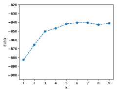
[]   $t=12$ m $t=24$ m RMSE RMSE RMSE RMSE 20-ahead 40-ahead 20-ahead 40-ahead BPsys 5.40 5.31 5.43 5.19 BPdia 3.63 3.79 3.55 3.75 BIS 7.42 7.35 7.68 7.81

Figure 12: Average (per patient) ELBO of MTPD model fitted on entire dataset for varying latent dimension $k$

Figure 13: Minimum possible predictive RMSE of PD model class. 20-, 40-step errors calculated in-sample for per-patient models after $t=12,24$.

5.3.4 LSTM Benchmark

It is unlikely that more complex/‘neural’ models such as RNNs will be accepted by practicing anaesthetists in the near future for a variety of reasons. The sample complexity of a RNN is poorly matched to the typical sample size of a clinical trial, predictions may perform very poorly under dataset shift (see Section 4.4.2), and the model is inscrutable, which precludes both an understanding of the prediction, and the ability to alter it. Nevertheless, it is still useful to provide a ‘neural’ benchmark to help us understand the opportunity cost of using simpler models. Note that if black box models are permissible, we might also expect improvements to RNNs using an MTDS approach (as in Section 4).

For the benchmark, we use a one-layer LSTM, with a hidden layer size of 32 and L2 regularization coefficient $10^{-3}$ chosen by grid search from $\{16,32,128\}$ $\times\,\{10^{-5},10^{-4},$ $10^{-3},10^{-2},10^{-1}\}$, and fitted via use of the Adam optimizer. As in Section 4 we train the model in an open-loop (or seq2seq) fashion, encoding 40 timesteps of inputs and outputs prior to a 40-step prediction. In each training iteration, the starting time $t$ is randomized. Observations with missing values required transformation for the ‘encoder’ section of the LSTM: these were handled by zero-imputation, concatenated with a one-hot encoding of the pattern of missingness.

5.4 Results

This section provides the experimental results, with an introduction in Section 5.4.1, and the leave-one-out results presented in Section 5.4.2.

Figure 14: Example predictions (mean and 90% CI) for BIS channel of a patient at $t=10,20,30$ minutes using Pooled-$\alpha$ and MTPD-5 models. The PK central compartment concentration is shown in the bottom panel. Retrospective fits are shown without intervals for clarity.

5.4.1 Introduction

Example predictions from both the MTPD-5 and Pooled-$\alpha$ models can be seen in Figure 14 for the BIS channel. One can see the models adapting over time at $t=10,20,30$ minutes, where the credible intervals show the predictive posterior for the underlying PD function. While the adaptive Pooled-$\alpha$ model (green) is fixed in shape and only updates its offset, the MTDS approach permits much greater flexibility, providing continual adaption over increasing $t$. Further examples can be seen in Bird et al. (2019, supplementary material).

Table 13 provides a lower bound of the error that can be achieved by the PD model class of Section 5.2.1 for the data in Section 5.3.1 via its in-sample error. To estimate this, we train a single-task model for each patient $i$ on the complete sequence $t=1,\ldots,T_{i}$ and report its in-sample error for 20-step and 40-step ahead predictions at $t=12,24$ as per Section 5.3. The RMSE of the BIS channel is relatively high, in part due to noise processes, but also since the PD model class is insufficiently flexible for this channel. For an example of BIS violating the PD model assumptions, see the step-change in the BIS channel observations at $t=30$ in Figure 14 which may perhaps correspond to a phase change in patient state (see e.g.  Mukamel et al. 2014) or some form of hysteresis.

5.4.2 Test set Results

The out-of-sample performance (LOO average) relative to the optimal performance (per the results in Table 13) is shown in Table 5 for all models. This is reported as Standardized RMSE (SRMSE), which is a ratio of the model RMSE to the optimal fit in Table 13. A value of $1.00$ indicates the same level of performance as the optimal PD fit, and a higher value indicates a worse fit. Results for the three channels are listed separately. One can see that the non-adaptive approaches often proposed in the literature (both Pooled and Task-ID) are highly suboptimal; for the blood pressure channels, the RMSE is more than twice that of the optimal fit.

			$t=12$ m			$t=24$ m
			SRMSE	SRMSE		SRMSE	SRMSE
			20-ahead	40-ahead		20-ahead	40-ahead
	Pooled		2.86	2.65		3.25	3.11
	Task-ID		2.84	2.64		3.23	3.10
	Pooled+$\alpha$		1.23	1.31		1.37	1.41
BPsys	Task-ID+$\alpha$		1.26	1.37		1.55	1.67
	STL		2.10	2.29		1.29	1.60
	MTDS-5		1.18	1.30		1.00	1.15
	MTDS-7		1.19	1.31		1.00	1.12
	LSTM (open loop)		1.59	1.76		1.46	1.48
	Pooled		2.42	2.37		2.59	2.35
	Task-ID		2.40	2.35		2.57	2.34
	Pooled+$\alpha$		1.03	1.13		1.21	1.15
BPdia	Task-ID+$\alpha$		1.16	1.30		1.23	1.24
	STL		1.50	1.74		1.57	1.58
	MTDS-5		1.12	1.24		1.01	1.03
	MTDS-7		1.15	1.25		1.02	0.99
	LSTM (open loop)		1.61	1.80		1.26	1.41
	Pooled		1.66	1.87		2.08	1.82
	Task-ID		1.69	1.90		2.11	1.84
	Pooled+$\alpha$		1.45	1.67		1.47	1.49
BIS	Task-ID+$\alpha$		1.66	2.01		1.65	1.69
	STL		1.97	3.16		1.31	1.61
	MTDS-5		1.35	1.81		1.21	1.29
	MTDS-7		1.32	1.85		1.19	1.28
	LSTM (open loop)		1.19	1.55		0.88	1.28

Table 5: The out-of-sample performance of each model standardized by the optimal PD results in Table 13 (lower is better). For each channel, models are split into standard PD approaches, adaptive PD approaches, and non-PD approaches. As per Table 13, the results give the 20 and 40-step predictive RMSE after $t=12,24$. The results highlighted in bold are the best performance from a PD model.

By $t=24$ there is a clear win for the MTDS models over all other PD approaches. The 20-step performance is essentially optimal for the BPsys and BPdia channels, and further, the performance is substantially better than the flexible black-box LSTM model. For BIS, an optimal performance is not achieved by any approach within the class of PD models, but the MTDS results are a promising step forward (for the LSTM results, see below). The ST approach performs relatively poorly for all channels, and inference takes 1-2 orders of magnitude longer than other approaches. Nevertheless, its performance is expected to improve with increasing $t$. The adaptive Pooled-$\alpha$ model performs better initially, but it is not flexible enough to provide much customization, and shows no improvement over time. The performance of the patient covariate model Task-ID (both adaptive and non) is similar to or worse than the Pooled version. While Task-ID models clearly suffer from overfitting, the in-sample improvement is fairly small, suggesting the available patient covariates may lack the required information to attain meaningful improvement. Note that patient covariates have already been used in the PK component, and are hence incorporated in the inputs.

There appears to be some performance advantage for using the LSTM model for the BIS channel (although the MTDS is able to reduce the gap by $t=24$). This may be due to the particularly serious mis-specification of the PD model for BIS, as mentioned above. The SRMSE of 0.88 for the BIS prediction at $t=24$ indicates that the LSTM can fit the data better than the in-sample PD model. In particular, the 1-d latent linear dynamics of the PD model cannot fit the stepped level changes and hysteresis sometimes observed. The latter results in correlated noise to the fit, which further misleads online inference for the MTDS. For further experimental results and discussion see Bird (2021), §6.

5.5 Conclusion

The application of the MTDS framework to PK/PD modelling problem provides a novel approach to personalized medicine, which (for our propofol data set) shows substantial promise over traditional approaches using patient covariates. For a novel patient, our approach initializes with a close approximation to the current state-of-the-art, but can achieve increasing personalization over time, without deviating from the model class accepted by clinical practitioners. This is performed via an efficient online Bayesian filtering approach, which reduces the risk of overfitting compared to a point estimate or amortized approach.

The experiments have highlighted a number of areas for further improvement. Firstly, the BIS channel may benefit from a more flexible PD model class. This can be seen from the relatively poor performance of optimal PD fits, visual inspection, and comparison with LSTM models. Secondly, model predictions can likely be improved via better experimental design of the infusion sequence. Finally, incorporating artefact models (see e.g. Quinn et al., 2009) should reduce the sensitivity of the inference to correlated noise and artefacts, reducing suboptimal predictions.

6 Conclusion

This paper has defined a new class of time series model: the multi-task dynamical system, together with methods of learning and inference. We have demonstrated the efficacy of these via two detailed experiments. Our results show that the MTDS can indeed learn an embedding of sequence characteristics, resulting in a family of dynamical systems which span the inter-sequence variation of the training set. This latent encoding can be used to personalize forecasts—leading to increased accuracy—or to modulate their characteristics at will, depending on the goals of an end user.

We believe that datasets containing multiple sequences often manifest the inter-sequence variation discussed in this paper. This extends to natural language or video data; other examples might often be found in a business context, albeit rarely in the public domain. If this belief is correct, predicting time series data accurately must require task inference (in the sense described here), unless one can use a separate model for each time series. For task inference, the only general-purpose alternatives to the MTDS are neural models (such as RNNs), which perform task inference implicitly. In contrast, our MTDS approach performs this explicitly and encompasses a number of existing models in the literature. We have shown a number of advantages of explicit inference in our experiments including interpretability, data efficiency, robustness to dataset shift, end-user control, and visualization.

Future work may consider extending the MTDS to handle non-stationary data explicitly via a time-varying dynamic task variable $\mathbf{z}_{t}$. Also, while the MTDS appears to interpolate well between tasks, it may not be able to extrapolate so well, as evidenced in Section 4.4.2. This can be handled by retraining, but it may be advantageous to consider extensions that can adapt faster to novel tasks.

Acknowledgments

The authors would like to thank Stefan Schraag, Shiona McKelvie, Mani Chandra and Nick Sutcliffe for the original study design and data collection for the drug response data. They also thank Ian Mason for making available the mocap data, as well as a helpful discussion. This work was supported by The Alan Turing Institute under the EPSRC grant EP/N510129/1.

A Further Details of General MTDS Models

In this section we provide further details about the construction of MTDS models.

A.1 Choice of Prior for Large $d$

For modern ‘neural’ applications, the dimension $d$ of the output space $\Theta=\mathbb{R}^{d}$, corresponding to the system and emission parameters, may be very large, e.g. ${\mathcal{O}}(10^{6})$ for RNNs. The parameter ${\bm{\phi}}$ will therefore be even larger; in the case of an affine $\mathbf{h}_{{\bm{\phi}}}$, the parameter will have $(k{+}1){\times}d$ dimensions, and for an MLP, ${\bm{\phi}}$ could be an order of magnitude larger even than this. Practical choices of prior will restrict the final layer of such an MLP to be relatively small, reducing the flexibility of this nonlinear approach. Nevertheless, use of an MLP may still be advantageous since, for example:

1. The MLP can result in non-Gaussian densities in parameter space, even if the manifold of the support is relatively simple.

2. A linear space of recurrent model parameters can yield highly non-linear changes even to simple dynamical systems via bifurcation (see e.g. Strogatz, 2018, §8). We speculate it might be advantageous to curve the manifold to avoid such phenomena.

3. More expressive choices may help utilization of the latent space (see e.g. Chen et al., 2017).

Nonetheless, it may often be reasonable to use a linear factor analysis model (i.e. $\mathbf{h}_{{\bm{\phi}}}$ is affine) when ${\bm{\theta}}$ is large. Empirically we have observed higher marginal likelihoods for smaller state space models when using a nonlinear manifold, but affine and nonlinear manifolds may work equally well for larger RNN models.

A.2 Use of Deterministic State Models

In this paper, we restrict our focus to deterministic state dynamical systems because the applications do not demand stochastic state models, and long-term predictions appear to benefit from the deterministic state. Some intuition of the latter can be found in Martinez et al. (2017) where use of a deterministic state forces the models to learn to ‘recover’ from their mistakes. Similar observations can be found in Bengio et al. (2015) or Chiappa et al. (2017) for example.

We also propose that the choice of deterministic state models is less limiting than it may first appear. Consider a simple linear dynamical system with no inputs:

$$\mathbf{x}_{t}\, =\,A\,\mathbf{x}_{t-1}+\mathbf{v}_{t},\qquad \mathbf{v}_{t}\sim\mathcal{N}\left(\mathbf{0},R\right),$$ (22)

$$\mathbf{y}_{t}\, =\,C\,\mathbf{x}_{t}+\mathbf{w}_{t},\qquad \mathbf{w}_{t}\sim\mathcal{N}\left(\mathbf{0},S\right).$$ (23)

Now consider a Kalman filter initialized from $p(\mathbf{x}_{t-1}|\mathbf{x}_{1\mathrel{\mathop{\mathchar 58\relax}}t-2})=\mathcal{N}(\mathbf{x}_{t-1}\,|\,\mathbf{m}_{t-1},\,P_{t-1})$ which infers the latent variables recursively (following Särkkä, 2013) via the following steps:

$$\mathbf{m}_{t}^{-} \,=\,A\mathbf{m}_{t-1},$$

$$P_{t}^{-} \,=\,AP_{t-1}A^{\mkern-1.5mu\mathsf{T}}+R.$$

$$K_{t} \,=\,P_{t}^{-}C^{\mkern-1.5mu\mathsf{T}}(CP_{t}^{-}C^{\mkern-1.5mu\mathsf{T}}+S)^{-1}.$$

$$\mathbf{m}_{t} \,=\,\mathbf{m}_{t}^{-}+K_{t}(\mathbf{y}_{t}-C\mathbf{m}_{t}^{-}),$$

$$P_{t} \,=\,P_{t}^{-}-K_{t}CP_{t}^{-}.$$

The conditional likelihood of the observations is $p(\mathbf{y}_{t}\,|\,\mathbf{y}_{1\mathrel{\mathop{\mathchar 58\relax}}t-1})\,=\,\mathcal{N}(C\mathbf{m}_{t}^{-}\,|\,CP_{t}^{-}C^{\mkern-1.5mu\mathsf{T}}+S)$, obtained from eq. (23). The covariance $P_{t}$ typically converges quickly to a fixed point (Barber, 2012, ch. 24), in which case the quantities $P_{t},K_{t}$ converge to time-independent quantities $P,K$ (for more details see Harvey, 1990, §3.3.3). Therefore at steady state the one-state conditional likelihoods can be described by the following system:

$$\mathbf{m}_{t} \,=\,A\mathbf{m}_{t-1}+K(\mathbf{y}_{t}-CA\mathbf{m}_{t-1})$$ (24)

$$\mathbf{y}_{t+1}\,|\,\mathbf{y}_{1\mathrel{\mathop{\mathchar 58\relax}}t} \,\sim\,\mathcal{N}\left(CA\mathbf{m}_{t},\,C(APA^{\mkern-1.5mu\mathsf{T}}+R)C^{\mkern-1.5mu\mathsf{T}}+S\right),$$ (25)

which is the form of a deterministic-state LDS. Hence for every stochastic-state LDS at steady state, there exists a deterministic-state LDS with the same distribution over $\mathbf{y}_{1\mathrel{\mathop{\mathchar 58\relax}}T}$. Notably however, the latter interprets the preceding observations $\mathbf{y}_{1\mathrel{\mathop{\mathchar 58\relax}}t-1}$ (at time $t$) as inputs, whereas the former may have no control inputs. While the steady-state assumption cannot always be made, this idea suggests that learning a deterministic LDS using observations $\mathbf{y}_{1\mathrel{\mathop{\mathchar 58\relax}}T-1}$ as inputs can approximate the likelihood of a stochastic model. Deterministic RNNs use a similar idea (sometimes called ‘teacher forcing’) which enables them to model notionally stochastic time series with high accuracy.

If one does wish to learn a stochastic state MTDS, the latent dynamical state must be integrated out for learning and inference over $\mathbf{z}$. This is a more difficult inference problem. Nevertheless, it is relatively easy to extend the MTDS to stochastic-state LDS models as this can be performed in closed form (as above), and the benefit of this closed-form inference may be further extended in principle to nonlinear models too as in e.g. Karl et al. (2017).

A.3 Implementations

An example implementation of the MTDS in PyTorch is provided at https://github.com/ornithos/pytorch-mtds-mocap, together with the data for the Mocap experiments. At the time of writing, the pharmacodynamic data is not yet publicly available, but a reference implementation of the model is available at https://gist.github.com/ornithos/71abb7349e91db633ce15971785bbae1.

A Julia implementation of AdaIS for performing sequential inference in models with static latent variables (such as the MTDS) can be found at https://github.com/ornithos/SeqAdaptiveIS.

B Application to Mocap Data

This section provides additional details pertaining to the mocap application in Section 4.

B.1 Model Inputs

Our choice of inputs reflects controls that an animator may wish to manipulate. The first input is the trajectory that the skeleton is to follow. As in Holden et al. (2017), we provide the trajectory over the next second (30 frames), sampled every 5 frames. Unlike previous work, the trajectory history of the prior 30 frames is omitted, since it can be retained in the dynamic state of the model. The (2-d) trajectory co-ordinates are given with respect to the Lagrangian co-ordinate frame, and hence can vary rapidly when the skeleton turns quickly. We choose to provide an Eulerian representation of the trajectory too, which sometimes resulted in a smoother prediction.

The velocity implied by the trajectory does not disambiguate the gait frequency vs. stride length. The same velocity may be achieved with fast short steps, or slower long strides. We therefore provide the gait frequency via a phasor (as in Holden et al., 2017). This is provided by sine and cosine components to avoid the discontinuity at $2\pi$. This may also be useful to an animator. A final ambiguity exists from the trajectory at tight corners: the skeleton can rotate either towards the focus of the corner, or in the opposite direction. Figure 4(b) demonstrates the latter, which is not infrequently performed in the data. We provide a boolean indicator for each of the 6 sampled trajectory timesteps, indicating corners for which this happens.

Altogether we have $\mathbf{u}_{t}\in\mathbb{R}^{35}$: 12 inputs each for the Lagrangian trajectory and the differenced Eulerian trajectory, 2 inputs for the gait phase, 6 inputs for the turning indicators and 3 additional inputs of the instantaneous velocity. These inputs $\{\mathbf{u}_{t}\}$ are standardized to have zero mean and unit variance. A particular problem in producing the inputs was the stylistic swaying/movement of the root joint which leaked information about the style in the trajectory and prevented customization of the pelvic movement. This was removed during pre-processing, for more on which see Bird (2021).

B.2 Recurrent Cell Definitions

Equations (13) and (14) refer to a GRUCell and a RNNCell which we define below.

$$\textrm{\small RNNCell}_{n_{x}}\left(\mathbf{x}_{t-1},\,\mathbf{u}_{t};\,\,\,{\bm{\psi}}\right)\,\mathrel{\mathop{\mathchar 58\relax}} =\,\tanh\left(A\mathbf{x}_{t-1}+B\mathbf{u}_{t}+\mathbf{b}\right),$$ (26)

where in this case $${\bm{\psi}} A\in\mathbb{R}^{n_{x}\times n_{x}},B\in\mathbb{R}^{n_{x}\times n_{u}},\mathbf{b}\in\mathbb{R}^{n_{x}}$$ comprises the parameters . The GRU cell can be written via the following four equations:

$$\textrm{\small GRUCell}_{n_{x}}\left(\mathbf{x}_{t-1},\,\mathbf{u}_{t};\,\,\,{\bm{\psi}}\right)\,\mathrel{\mathop{\mathchar 58\relax}} =\,(1-\mathbf{g}^{s}_{t})\odot\mathbf{x}_{t-1}+\mathbf{g}^{s}_{t}\odot\hat{\mathbf{x}}_{t},$$

$$\hat{\mathbf{x}}_{t} \,=\,\tanh\left(A^{\mathbf{x}}\mspace{1.0mu}(\mathbf{g}^{r}_{t}\odot\mathbf{x}_{t-1})+B^{\mathbf{x}}\mspace{1.0mu}\mathbf{u}_{t}+\mathbf{b}^{\mathbf{x}}\right)$$

$$\mathbf{g}^{r}_{t} \,=\,\bm{\sigma}\left(A^{r}\mspace{1.0mu}\mathbf{x}_{t-1}+B^{r}\mspace{1.0mu}\mathbf{u}_{t}+\mathbf{b}^{r}\right)$$

$$\mathbf{g}^{s}_{t} \,=\,\bm{\sigma}\left(A^{s}\mspace{1.0mu}\mathbf{x}_{t-1}+B^{s}\mspace{1.0mu}\mathbf{u}_{t}+\mathbf{b}^{s}\right),$$

where $\odot$ represents elementwise multiplication and ${\bm{\psi}}$ comprises the parameters $A^{r},A^{s},A^{\mathbf{x}}\in\mathbb{R}^{n_{x}\times n_{x}},\,B^{r},B^{s},B^{\mathbf{x}}\in\mathbb{R}^{n_{x}\times n_{u}},\,\mathbf{b}^{r},\mathbf{b}^{s},\mathbf{b}^{\mathbf{x}}\in\mathbb{R}^{n_{x}}$.

B.3 Additional Learning Details

Model	Optimizer	$\eta$	Multi-task $\eta$	Regularization
MT-RNN	Adam	$3\times 10^{-5}$	$1\times 10^{-3}$	$1\times 10^{-2}$
GRU-1L (closed loop)	Adam	$5\times 10^{-4}$	-	$5\times 10^{-4}$
GRU-2L (closed loop)	Adam	$1\times 10^{-4}$	-	$5\times 10^{-4}$
GRU-1L (open loop)	Adam	$5\times 10^{-4}$	-	0
GRU-2L (open loop)	Adam	$1\times 10^{-4}$	-	0

Table 6: Hyper-parameters of mocap models. $\eta$ denotes the learning rate.

MTDS, MT-Bias models:

Each sequence was broken into overlapping segments of length 64 (approx. two second intervals), with a different $\mathbf{z}$ per segment. Unlike open-loop training in Martinez et al. (2017), predictions do not use the previous modelled output $\hat{\mathbf{y}}_{t-1}$ when predicting the following time step. This is required in previous work since the observations $\mathbf{y}_{1\mathrel{\mathop{\mathchar 58\relax}}T_{\textrm{\scriptsize enc}}}$ are required as inputs in the encoding stage, and hence predictions are used in their place for the decoding stage. By use of an explicit latent $\mathbf{z}$, we avoid the need to perform encoding via the sequence model, and hence avoid the need to append the predictions to the inputs; the information from the inputs is already contained in the recurrent state.

The model was optimized for 20 000 iterations with $N_{\textrm{batch}}=16$ using the variational procedure in Section 2.2. We used standard variational inference for each $\mathbf{z}^{(i)}$ (i.e. each posterior is parameterized directly), which worked better in general than amortized inference using an inference network. A form of KL annealing (Bowman et al., 2016) was also used for improving the quality of the latent description. Hyperparameters were chosen primarily via the ELBO, but the qualitative training set fit was also considered where values were similar; specifically we compared the smoothness of animation, and the results of style transfer on a few candidate tasks. The choices are shown in Table 6. The main learning rate $\eta$ applies to the fixed parameters wrt. $\mathbf{z}$ (i.e. ${\bm{\psi}}_{1},H$), and the multi-task learning rate applies to the parameter generation parameters ${\bm{\phi}}$ (i.e. ${\bm{\psi}}_{1},H,C_{1}$) and inference parameters ${\bm{\lambda}}$. L2 regularization was applied to ${\bm{\phi}},{\bm{\psi}}_{1},H$. Models were learned for $k=3,5,7,9$, for which the optimal choice via the ELBO varied across experiments, but was most frequently either $k=5$ or 7. We report multiple values in the results to give the reader some insight into the importance of this hyperparameter. The model was implemented in PyTorch (Paszke et al., 2017) and trained on an NVIDIA K80 GPU.

Benchmark Models:

The models are trained on predicting length 64 sequences (chosen at random at each iteration), using the encoding from the previous $T_{\textrm{\scriptsize enc}}=64$ frames. The hyper-parameters were chosen using a grid search over learning rate, regularization, and optimizer {Adam, SGD}. We perform the search over the pooled data for all 8 styles, with a stratified sample of 12.5% held out for a validation set. The benchmark models were trained for a maximum of 20 000 iterations with early stopping. See Table 6 for the chosen hyperparameters.

B.4 Additional Details of Results

This section provides further details of the qualitative results: the latent representation (Section B.4.1) and style transfer experiment (Section B.4.2)

B.4.1 Qualitative Representation

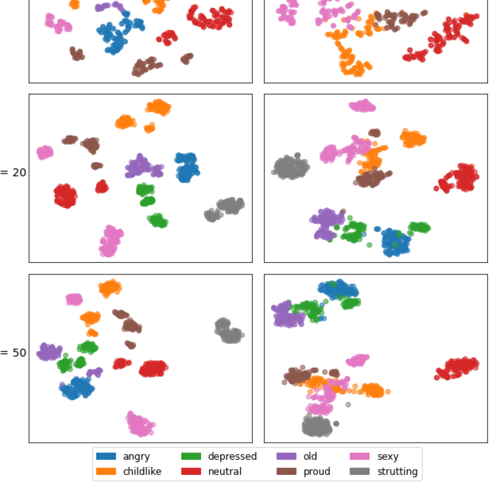
Figure 15: Mean embedding of latent $\mathbf{z}$ coloured by true style of the proposed MTDS model vs. a MT-Bias approach. Figure shows t-SNE plot for perplexity 20. The original $\mathbf{z}$ data have $k=8$ dimensions, and are standardized to have zero mean, unit variance.

Figure 15 compares the t-SNE embeddings for the MTDS and MT-Bias models. The MTDS maintains well-defined clusters for different styles, which are not only homogeneous in terms of the original style label, but obtain a further split into qualitatively different sub-styles. In the MT-Bias case, there are many clusters which ‘bleed into each other’. This means that some differing styles are closer to each other in latent space than some instances of the same style. The representation of the sub-styles is also much weaker. These observations are valid for all values of the ‘perplexity’ parameter in t-SNE, except for small values where little-to-no clustering occurs.

B.4.2 Style Transfer

Experimental Setup:

We pre-process the mocap sequences to standardize the gait frequency across all styles; some styles can be identified purely by calculating the frequency. It is critical for these experiments that the classifier cannot use this information. All sequences are standardized to use the inter-style mean frequency (1 cycle per 33 frames, or 1.1 Hz), which is applied via linear interpolation. This process is made straight-forward by the presence of the phase given in the input sequence $U$.

The experimental setup is as follows. We choose four segments of length 64 for each of the styles $s_{1}=1,\ldots,8$, being careful to represent the variability within each style. These segments are used as the input data $U_{j}^{(s_{1})}$ for each source style $s_{1}$ with $j=1,\ldots,4$ examples. We next seek the ‘canonical’ latent code $\mathbf{z}$ to be associated with each target style $s_{2}$. To this end, we consider the posterior mean ($\mathchoice{\bm{\mu}_{\raisebox{-0.8pt}{\scalebox{0.7}{$\displaystyle{\bm{\lambda}}$}}}}{\bm{\mu}_{\raisebox{-0.8pt}{\scalebox{0.7}{$\textstyle{\bm{\lambda}}$}}}}{\bm{\mu}_{\raisebox{-0.8pt}{\scalebox{0.7}{$\scriptstyle{\bm{\lambda}}$}}}}{\bm{\mu}_{\raisebox{-0.8pt}{\scalebox{0.7}{$\scriptscriptstyle{\bm{\lambda}}$}}}}$) of each training sequence in ${\mathcal{D}}$, but since many styles have multiple clusters (as can be seen in Figure 8), the mean of the $\{\mathchoice{\bm{\mu}_{\raisebox{-0.8pt}{\scalebox{0.7}{$\displaystyle{\bm{\lambda}}$}}}}{\bm{\mu}_{\raisebox{-0.8pt}{\scalebox{0.7}{$\textstyle{\bm{\lambda}}$}}}}{\bm{\mu}_{\raisebox{-0.8pt}{\scalebox{0.7}{$\scriptstyle{\bm{\lambda}}$}}}}{\bm{\mu}_{\raisebox{-0.8pt}{\scalebox{0.7}{$\scriptscriptstyle{\bm{\lambda}}$}}}}\}$ within each style may therefore not correspond to any existing style. We circumvent this problem by optimizing the latent code $\mathbf{z}^{(s_{2})}$ as a discrete choice from among the relevant $\{\mathchoice{\bm{\mu}_{\raisebox{-0.8pt}{\scalebox{0.7}{$\displaystyle{\bm{\lambda}}$}}}}{\bm{\mu}_{\raisebox{-0.8pt}{\scalebox{0.7}{$\textstyle{\bm{\lambda}}$}}}}{\bm{\mu}_{\raisebox{-0.8pt}{\scalebox{0.7}{$\scriptstyle{\bm{\lambda}}$}}}}{\bm{\mu}_{\raisebox{-0.8pt}{\scalebox{0.7}{$\scriptscriptstyle{\bm{\lambda}}$}}}}\}$, choosing the value that performs the best at our style transfer task. The 32 highly varied input sequences guard against overfitting—the ‘canonical’ latent codes for each style must perform well for all styles and sub-styles; the majority of the variability of the original dataset. We perform this independently for both the MT-Bias and MTDS model.

We provide a scalar measurement of the ‘success’ of style transfer for each pair ($s_{1}$, $s_{2}$) by using the resulting ‘probability’ that the classifier assigns the target style $s_{2}$, averaged across the four input sequences for the source $s_{1}$. A score of 1.00 thus requires the classifier to output a highly certain prediction of the target style $s_{2}$ for all of the 32 different input sequences $\{U_{j}^{(s_{1})}\}$.

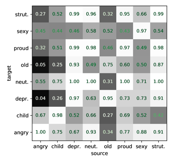
(a) MT-Bias

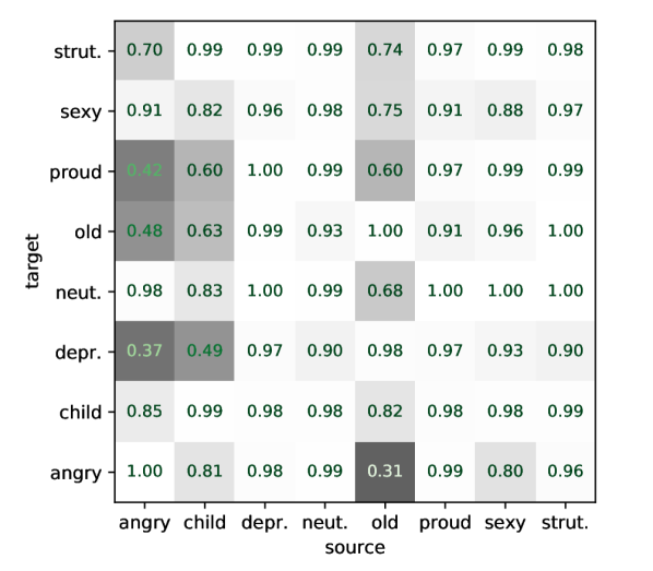
(b) MTDS

Figure 16: Average classification accuracy for style transfer using inputs from source style (columns) and latent code $\mathbf{z}$ from target style (rows). There is no style transfer on the diagonal.

(a) MT-Bias

(b) MTDS

Figure 17: Average classification accuracy for style transfer where only a single source input is used for each (source, target) pair. The configuration of the matrix is the same as Figure 16.

Results Breakdown:

The breakdown of these results into their (source, target) pairs are given in Figure 16. The cells provide the average classifier probability for the target style over each combination (averaged over the four source sequences). Successful style transfer should result in a high score in every cell. For most (source, target) pairs, the full MTDS model substantially outperforms the MT-Bias model, resulting in superior user control in the majority of cases. We can gain some insight into the MT-Bias performance via its latent representation (Figure 15), where we see it has conflated a variety of styles, which are disambiguated therefore only via the inputs. It is therefore not surprising that changing the latent $\mathbf{z}$ often results in unrecognizable changes.

It is notable that both models exhibit worse results when styles are associated with extremes of the input distribution. Specifically, both the ‘childlike’ and ‘angry’ styles have unusually fast trajectories, and the ‘old’ style has unusually slow ones. The lowest scores tend to involve these styles as either the source or the target. This suggests that the first layer (GRU) fails to provide a coherent shared representation of these behaviours, and/or there is some information leakage from the inputs. We leave further investigation and improvements to future work.

Providing style transfer from a wide variety of source styles is a challenging task. We are attempting to find a single latent code which can reliably transfer style from 28 different source sequences, many of which may be mismatched to the target style. We consider a more pragmatic experiment where the variety of source styles is reduced to a single example each. Nonetheless, the same $\mathbf{z}^{(s_{2})}$ is used across all sources $s_{1}$. The results of this secondary experiment are provided in Figure 17. In this case, the MTDS achieves successful style transfer for almost all (source, target) combinations. The MT-Bias model still has many notable failures.

C Application to drug response data

In this section we provide additional details pertaining to the pharmacodynamic application in Section 5.

C.1 Data: Infusion Sequences

The $N=40$ patients are split into two groups, each of which is given a different intravenous schedule of propofol. The two different schedules split the time into three consecutive segments of 10-15 minutes each, within which the TCI pump targeted a high-low-high, or a low-high-low concentration of propofol. The two schedules are visualized in Figure 18 using the propofol concentration predicted via the White et al. (2008) model.

C.2 Derivation of Discrete-Time Relationship for Piecewise Constant $\mathbf{u}(t)$

Equation (16) can be solved by integration using Laplace transformations. Let $U(s)$ be the Laplace transform of $c(t)$, and $X(s)$ the Laplace transform of $x(t)$. Define further a piecewise constant $u(t)=\sum_{i=0}^{T-1}R(t-i)u_{i}$ with a slight abuse of notation for $u$, and for $R(\cdot)$ the unit rectangle function. Then we have:

$$sX(s) =k_{1e}U(s)-k_{e0}X(s)$$ (27)

$$\Rightarrow X(s) =\frac{k_{1e}U(s)}{s+k_{e0}}.$$ (28)

Recognising the RHS as the product of two known Laplace transformations gives:

$$\mathcal{L}(x(t)) =\mathcal{L}(k_{1e}u(t))\cdot\mathcal{L}(e^{-k_{e0}t}H(t))$$ (29)

for the Heaviside step function $$H(t)$$. Then using the convolution theorem:

$$\Rightarrow x(t) =k_{1e}\int_{0}^{t}e^{-k_{e0}\tau}u(t-\tau)\operatorname{d\!}\tau$$ (30)

$$=k_{1e}\left[\sum_{i=0}^{t-1}u_{i}\int_{0}^{t}e^{-k_{e0}\tau}R(t-\tau-i)\operatorname{d\!}\tau\right]$$ (31)

$$=k_{1e}\left[\sum_{i=0}^{t-1}u_{i}\int_{t-i-1}^{t-i}e^{-k_{e0}\tau}\operatorname{d\!}\tau\right]$$ (32)

$$=k_{1e}\sum_{i=0}^{t-1}u_{i}\frac{1}{k_{e0}}\left[e^{-k_{e0}(t-i-1)}-e^{-k_{e0}(t-i)}\right]$$ (33)

$$=\sum_{i=0}^{t-1}\frac{k_{1e}}{k_{e0}}u_{i}\left(1-e^{-k_{e0}}\right)e^{-k_{e0}(t-i-1)}$$ (34)

$$=\frac{k_{1e}}{k_{e0}}\left(1-e^{-k_{e0}}\right)\sum_{i=0}^{t-1}u_{i}(e^{-k_{e0}})^{t-i-1}.$$ (35)

Equation (18) can be written explicitly as $x_{tj}=\beta_{1j}\sum_{i=0}^{t-1}\beta_{2j}^{t-i-1}u_{i}$ by unrolling the recursion. The relationships given in Section 5.2.1 are then derived by comparison with eq. (35).

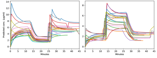
Figure 18: Predictions of White et al. (2008) PK model for each of the 40 patients, split by infusion schedule type: (left) high-low-high, (right) low-high-low. The inter-individual differences seen here are primarily due to the raw infusion chosen by the anaesthetist, rather than the modelled inter-patient variation.

References

- Alaa et al. (2018) Ahmed M Alaa, Jinsung Yoon, Scott Hu, and Mihaela van der Schaar. Personalized Risk Scoring for Critical Care Prognosis using Mixtures of Gaussian Processes. IEEE Transactions on Biomedical Engineering, 65(1):207–218, 2018.
- Álvarez et al. (2012) Mauricio A Álvarez, Lorenzo Rosasco, and Neil D Lawrence. Kernels for Vector-Valued Functions: A Review. Foundations and Trends® in Machine Learning, 4(3):195–266, 2012.
- Álvarez et al. (2013) Mauricio A Álvarez, David Luengo, and Neil D Lawrence. Linear Latent Force Models Using Gaussian Processes. IEEE Transactions on Pattern Analysis and Machine Intelligence, 35:2693–2705, 2013.
- Ando and Zhang (2005) Rie Kubota Ando and Tong Zhang. A Framework for Learning Predictive Structures from Multiple Tasks and Unlabeled Data. Journal of Machine Learning Research, 6(Nov):1817–1853, 2005.
- Aström and Murray (2010) Karl Johan Aström and Richard M Murray. Feedback Systems: an Introduction for Scientists and Engineers. Princeton University Press, 2010.
- Bailey and Haddad (2005) James M Bailey and Wassim M Haddad. Drug Dosing Control in Clinical Pharmacology. IEEE Control Systems, 25(2):35–51, 2005.
- Bakker and Heskes (2003) Bart Bakker and Tom Heskes. Task Clustering and Gating for Bayesian Multitask Learning. Journal of Machine Learning Research, 4(May):83–99, 2003.
- Barber (2012) David Barber. Bayesian Reasoning and Machine Learning. Cambridge University Press, 2012.
- Bengio et al. (2015) Samy Bengio, Oriol Vinyals, Navdeep Jaitly, and Noam Shazeer. Scheduled Sampling for Sequence Prediction with Recurrent Neural Networks. In Advances in Neural Information Processing Systems (NeurIPS) 29, pages 1171–1179, 2015.
- Bird (2021) Alex Bird. Multi-Task Dynamical Systems. PhD thesis, School of Informatics, University of Edinburgh, 2021. URL https://era.ed.ac.uk/handle/1842/38267.
- Bird et al. (2019) Alex Bird, Christopher K. I. Williams, and Christopher Hawthorne. Multi-Task Time Series Analysis applied to Drug Response Modelling. In International Conference on Artificial Intelligence and Statistics (AISTATS), 2019.
- Bonilla et al. (2008) E. Bonilla, K. M. A. Chai, and C. K. I. Williams. Multi-task Gaussian Process Prediction. In J.C. Platt, D. Koller, Y. Singer, and S. Roweis, editors, Advances in Neural Information Processing Systems (NeurIPS) 21. MIT Press, Cambridge, MA, 2008.
- Bowman et al. (2016) Samuel Bowman, Luke Vilnis, Oriol Vinyals, Andrew M Dai, Rafal Jozefowicz, and Samy Bengio. Generating Sentences from a Continuous Space. In Conference on Computational Natural Language Learning (CoNLL), 2016.
- Burda et al. (2016) Yuri Burda, Roger Grosse, and Ruslan Salakhutdinov. Importance Weighted Autoencoders. In International Conference on Learning Representations (ICLR), 2016.
- Cappé et al. (2008) Olivier Cappé, Randal Douc, Arnaud Guillin, Jean-Michel Marin, and Christian P Robert. Adaptive Importance Sampling in General Mixture Classes. Statistics and Computing, 18(4):447–459, 2008.
- Carpenter et al. (2016) Bob Carpenter, Andrew Gelman, Matt Hoffman, Daniel Lee, Ben Goodrich, Michael Betancourt, Michael A Brubaker, Jiqiang Guo, Peter Li, Allen Riddell, et al. Stan: A Probabilistic Programming Language. Journal of Statistical Software, 20(2):1–37, 2016.
- Caruana (1998) R Caruana. Multitask Learning. PhD thesis, Carnegie Mellon University, 1998.
- Chen et al. (2017) Xi Chen, Diederik P Kingma, Tim Salimans, Yan Duan, Prafulla Dhariwal, John Schulman, Ilya Sutskever, and Pieter Abbeel. Variational Lossy Autoencoder. In International Conference on Learning Representations (ICLR), 2017.
- Cheng et al. (2020) Li-Fang Cheng, Bianca Dumitrascu, Michael Zhang, Corey Chivers, Michael Draugelis, Kai Li, and Barbara Engelhardt. Patient-Specific Effects of Medication Using Latent Force Models with Gaussian Processes. In International Conference on Artificial Intelligence and Statistics (AISTATS), 2020.
- Chiappa and Barber (2007) Silvia Chiappa and David Barber. Output Grouping using Dirichlet Mixtures of Linear Gaussian State-Space Models. In International Symposium on Image and Signal Processing and Analysis. IEEE, 2007.
- Chiappa et al. (2017) Silvia Chiappa, Sébastien Racaniere, Daan Wierstra, and Shakir Mohamed. Recurrent Environment Simulators. In International Conference on Learning Representations (ICLR), 2017.
- Cho et al. (2014) Kyunghyun Cho, Bart van Merrienboer, Caglar Gulcehre, Dzmitry Bahdanau, Fethi Bougares, Holger Schwenk, and Yoshua Bengio. Learning Phrase Representations using RNN Encoder–Decoder for Statistical Machine Translation. In Conference on Empirical Methods in Natural Language Processing (EMNLP), 2014.
- Chopin (2002) Nicolas Chopin. A Sequential Particle Filter Method for Static Models. Biometrika, 89(3):539–552, 2002.
- Chopin et al. (2013) Nicolas Chopin, Pierre E Jacob, and Omiros Papaspiliopoulos. SMC2: an Efficient Algorithm for Sequential Analysis of State Space Models. Journal of the Royal Statistical Society: Series B (Statistical Methodology), 75(3):397–426, 2013.
- De la Torre et al. (2009) Fernando De la Torre, Jessica Hodgins, Adam Bargteil, Xavier Martin, Justin Macey, Alex Collado, and Pep Beltran. Guide to the Carnegie Mellon University Multimodal Activity (CMU-MMAC) Database. 2009.
- Denton and Birodkar (2017) Emily L Denton and Vighnesh Birodkar. Unsupervised Learning of Disentangled Representations from Video. In Advances in Neural Information Processing Systems (NeurIPS) 30, pages 4414–4423. 2017.
- Doucet et al. (2000) Arnaud Doucet, Simon Godsill, and Christophe Andrieu. On Sequential Monte Carlo Sampling Methods for Bayesian Filtering. Statistics and Computing, 10(3), 2000.
- Dürichen et al. (2015) Robert Dürichen, Marco AF Pimentel, Lei Clifton, Achim Schweikard, and David A Clifton. Multitask Gaussian Processes for Multivariate Physiological Time-Series Analysis. IEEE Transactions on Biomedical Engineering, 62(1):314–322, 2015.
- Eleveld et al. (2018) DJ Eleveld, P Colin, AR Absalom, and MMRF Struys. Pharmacokinetic–Pharmacodynamic Model for Propofol for Broad Application in Anaesthesia and Sedation. British Journal of Anaesthesia, 120(5):942–959, 2018.
- Fabius and van Amersfoort (2015) Otto Fabius and Joost R van Amersfoort. Variational Recurrent Auto-encoders. In International Conference on Learning Representations (ICLR), 2015.
- Fragkiadaki et al. (2015) Katerina Fragkiadaki, Sergey Levine, Panna Felsen, and Jitendra Malik. Recurrent Network Models for Human Dynamics. In IEEE International Conference on Computer Vision (ICCV), pages 4346–4354, 2015.
- Futoma et al. (2016) Joseph Futoma, Mark Sendak, Blake Cameron, and Katherine Heller. Predicting Disease Progression with a Model for Multivariate Longitudinal Clinical Data. In Machine Learning for Healthcare Conference, 2016.
- Georgatzis et al. (2016) Konstantinos Georgatzis, Christopher K. I. Williams, and Christopher Hawthorne. Input-Output Non-Linear Dynamical Systems applied to Physiological Condition Monitoring. Machine Learning for Healthcare, 2016.
- Ghosh et al. (2017) Partha Ghosh, Jie Song, Emre Aksan, and Otmar Hilliges. Learning Human Motion Models for Long-Term Predictions. In IEEE International Conference on 3D Vision (3DV), pages 458–466, 2017.
- Gilks and Berzuini (2001) Walter R Gilks and Carlo Berzuini. Following a Moving Target – Monte Carlo Inference for Dynamic Bayesian Models. Journal of the Royal Statistical Society: Series B (Statistical Methodology), 63(1):127–146, 2001.
- Glen and White (2014) JB Glen and M White. A Comparison of the Predictive Performance of Three Pharmacokinetic Models for Propofol Using Measured Values Obtained During Target-Controlled Infusion. Anaesthesia, 69(6):550–557, 2014.
- Goodfellow et al. (2016) Ian Goodfellow, Yoshua Bengio, and Aaron Courville. Deep Learning. MIT Press, 2016.
- Goyal et al. (2017) Anirudh Goyal, Alessandro Sordoni, Marc-Alexandre Côté, Nan Rosemary Ke, and Yoshua Bengio. Z-Forcing: Training Stochastic Recurrent Networks. In Advances in Neural Information Processing Systems (NeurIPS) 31, pages 6713–6723, 2017.
- Harvey (1990) Andrew C Harvey. Forecasting, Structural Time Series Models and the Kalman Filter. Cambridge University Press, 1990.
- Hochreiter and Schmidhuber (1997) Sepp Hochreiter and Jürgen Schmidhuber. Long Short-Term Memory. Neural Computation, 9(8):1735–1780, 1997.
- Hoffman and Gelman (2014) Matthew D Hoffman and Andrew Gelman. The No-U-Turn Sampler: Adaptively Setting Path Lengths in Hamiltonian Monte Carlo. Journal of Machine Learning Research, 15(1):1593–1623, 2014.
- Holden et al. (2016) Daniel Holden, Jun Saito, and Taku Komura. A Deep Learning Framework for Character Motion Synthesis and Editing. ACM Transactions on Graphics (TOG), 35(4):138, 2016.
- Holden et al. (2017) Daniel Holden, Taku Komura, and Jun Saito. Phase-Functioned Neural Networks for Character Control. ACM Transactions on Graphics (TOG), 36(4):42, 2017.
- Holford (2018) Nick Holford. Pharmacodynamic Principles and the Time Course of Delayed and Cumulative Drug Effects. Translational and Clinical Pharmacology, 26(2):56–59, 2018.
- Hsieh et al. (2018) Jun-Ting Hsieh, Bingbin Liu, De-An Huang, Li F Fei-Fei, and Juan Carlos Niebles. Learning to Decompose and Disentangle Representations for Video Prediction. In Advances in Neural Information Processing Systems (NeurIPS) 31, pages 517–526, 2018.
- Hsu et al. (2017) Wei-Ning Hsu, Yu Zhang, and James Glass. Unsupervised Learning of Disentangled and Interpretable Representations from Sequential Data. In Advances in Neural Information Processing Systems (NeurIPS) 30, pages 1876–1887. 2017.
- Hüppe et al. (2019) Tobias Hüppe, Felix Maurer, Daniel I. Sessler, Thomas Volk, and Sascha Kreuer. Retrospective comparison of Eleveld, Marsh, and Schnider propofol pharmacokinetic models in 50 patients. British Journal of Anaesthesia, 2019.
- Inoue et al. (2007) Lurdes YT Inoue, Mauricio Neira, Colleen Nelson, Martin Gleave, and Ruth Etzioni. Cluster-Based Network Model for Time-Course Gene Expression Data. Biostatistics, 8:507–525, 2007.
- Jeleazcov et al. (2015) Christian Jeleazcov, Marc Lavielle, Jürgen Schüttler, and Harald Ihmsen. Pharmacodynamic Response Modelling of Arterial Blood Pressure in Adult Volunteers During Propofol Anaesthesia. British Journal of Anaesthesia, 115(2):213–226, 2015.
- Karl et al. (2017) Maximilian Karl, Maximilian Soelch, Justin Bayer, and Patrick van der Smagt. Deep Variational Bayes Filters: Unsupervised Learning of State Space Models from Raw Data. In International Conference on Learning Representations (ICLR), 2017.
- Kingma and Welling (2014) Diederik P Kingma and Max Welling. Stochastic Gradient VB and the Variational Auto-Encoder. In International Conference on Learning Representations (ICLR), 2014.
- Le et al. (2018) Tuan Anh Le, Maximilian Igl, Tom Rainforth, Tom Jin, and Frank Wood. Auto-Encoding Sequential Monte Carlo. In International Conference on Learning Representations (ICLR), 2018.
- Lee and Grimson (2002) Lily Lee and W Eric L Grimson. Gait Analysis for Recognition and Classification. In IEEE International Conference on Automatic Face Gesture Recognition. IEEE, 2002.
- Lin et al. (2019) Alexander Lin, Yingzhuo Zhang, Jeremy Heng, Stephen A Allsop, Kay M Tye, Pierre E Jacob, and Demba Ba. Clustering Time Series with Nonlinear Dynamics: A Bayesian Non-Parametric and Particle-Based Approach. In International Conference on Artificial Intelligence and Statistics (AISTATS), 2019.
- Linderman et al. (2017) Scott Linderman, Matthew Johnson, Andrew Miller, Ryan Adams, David Blei, and Liam Paninski. Bayesian Learning and Inference in Recurrent Switching Linear Dynamical Systems. In International Conference on Artificial Intelligence and Statistics (AISTATS), pages 914–922, 2017.
- Lobo and Schraag (2011) Francisco A Lobo and Stefan Schraag. Limitations of Anaesthesia Depth Monitoring. Current Opinion in Anesthesiology, 24(6):657–664, 2011.
- Maddison et al. (2017) Chris J Maddison, John Lawson, George Tucker, Nicolas Heess, Mohammad Norouzi, Andriy Mnih, Arnaud Doucet, and Yee Teh. Filtering Variational Objectives. In Advances in Neural Information Processing Systems (NeurIPS) 31, pages 6573–6583, 2017.
- Mager et al. (2003) Donald E Mager, Elzbieta Wyska, and William J Jusko. Diversity of Mechanism-Based Pharmacodynamic Models. Drug Metabolism and Disposition, 31(5):510–518, 2003.
- Marsh et al. (1991) B Marsh, M White, N Morton, and GNC Kenny. Pharmacokinetic Model Driven Infusion of Propofol in Children. British Journal of Anaesthesia, 67(1):41–48, 1991.
- Martinez et al. (2017) Julieta Martinez, Michael J Black, and Javier Romero. On Human Motion Prediction Using Recurrent Neural Networks. In IEEE Conference on Computer Vision and Pattern Recognition (CVPR), pages 2891–2900, 2017.
- Mason et al. (2018) Ian Mason, Sebastian Starke, He Zhang, Hakan Bilen, and Taku Komura. Few-Shot Learning of Homogeneous Human Locomotion Styles. In Computer Graphics Forum, volume 37, pages 143–153. Wiley Online Library, 2018.
- Masui et al. (2010) Kenichi Masui, Richard N Upton, Anthony G Doufas, Johan F Coetzee, Tomiei Kazama, Eric P Mortier, and Michel M Struys. The Performance of Compartmental and Physiologically Based Recirculatory Pharmacokinetic Models for Propofol: a Comparison Using Bolus, Continuous, and Target-Controlled Infusion Data. Anesthesia & Analgesia, 111(2):368–379, 2010.
- Memisevic and Hinton (2007) Roland Memisevic and Geoffrey Hinton. Unsupervised Learning of Image Transformations. In IEEE Conference on Computer Vision and Pattern Recognition (CVPR), pages 1–8. IEEE, 2007.
- Memisevic and Hinton (2010) Roland Memisevic and Geoffrey E Hinton. Learning to Represent Spatial Transformations with Factored Higher-Order Boltzmann Machines. Neural Computation, 22(6):1473–1492, 2010.
- Miladinović et al. (2019) Đorđe Miladinović, Muhammad Waleed Gondal, Bernhard Schölkopf, Joachim M. Buhmann, and Stefan Bauer. Disentangled State Space Representations. arXiv e-prints, art. 1906.03255, Jun 2019.
- Mukamel et al. (2014) Eran A Mukamel, Elvira Pirondini, Behtash Babadi, Kin Foon Kevin Wong, Eric T Pierce, P Grace Harrell, John L Walsh, Andres F Salazar-Gomez, Sydney S Cash, Emad N Eskandar, et al. A Transition in Brain State During Propofol-Induced Unconsciousness. Journal of Neuroscience, 34(3):839–845, 2014.
- Myles et al. (2004) PS Myles, K Leslie, J McNeil, A Forbes, MTV Chan, B-Aware Trial Group, et al. Bispectral Index Monitoring to Prevent Awareness During Anaesthesia: the B-Aware Randomised Controlled Trial. The Lancet, 363(9423):1757–1763, 2004.
- Naesseth et al. (2018) Christian Naesseth, Scott Linderman, Rajesh Ranganath, and David Blei. Variational Sequential Monte Carlo. In International Conference on Artificial Intelligence and Statistics (AISTATS), pages 968–977, 2018.
- Opper and Winther (1998) Manfred Opper and Ole Winther. A Bayesian Approach to Online Learning. On-line Learning in Neural Networks, 6:363–378, 1998.
- Osborne et al. (2008) Michael A Osborne, Stephen J Roberts, Alex Rogers, Sarvapali D Ramchurn, and Nicholas R Jennings. Towards Real-Time Information Processing of Sensor Network Data Using Computationally Efficient Multi-Output Gaussian Processes. In International Conference on Information Processing in Sensor Networks, pages 109–120. IEEE Computer Society, 2008.
- Owen (2013) Art B. Owen. Monte Carlo Theory, Methods and Examples. 2013. Published online at time of writing, retrieved from https://artowen.su.domains/mc/.
- Paszke et al. (2017) Adam Paszke, Sam Gross, Soumith Chintala, Gregory Chanan, Edward Yang, Zachary DeVito, Zeming Lin, Alban Desmaison, Luca Antiga, and Adam Lerer. Automatic Differentiation in PyTorch. 2017.
- Pavllo et al. (2018) Dario Pavllo, David Grangier, and Michael Auli. Quaternet: A Quaternion-Based Recurrent Model for Human Motion. In British Machine Vision Conference (BMVC), 2018.
- Quinn et al. (2009) John A Quinn, Christopher K I Williams, and Neil McIntosh. Factorial Switching Linear Dynamical Systems applied to Physiological Condition Monitoring. IEEE Transactions on Pattern Analysis and Machine Intelligence, 31(9):1537–1551, 2009.
- Rangapuram et al. (2018) Syama Sundar Rangapuram, Matthias W Seeger, Jan Gasthaus, Lorenzo Stella, Yuyang Wang, and Tim Januschowski. Deep State Space Models for Time Series Forecasting. In Advances in Neural Information Processing Systems (NeurIPS) 31, pages 7785–7794, 2018.
- Rezende et al. (2014) Danilo Jimenez Rezende, Shakir Mohamed, and Daan Wierstra. Stochastic Backpropagation and Approximate Inference in Deep Generative Models. In International Conference on Machine Learning (ICML), pages 1278–1286, 2014.
- Roberts et al. (2013) Stephen Roberts, Michael Osborne, Mark Ebden, Steven Reece, Neale Gibson, and Suzanne Aigrain. Gaussian Processes for Time-Series Modelling. Philosophical Transactions of the Royal Society A: Mathematical, Physical and Engineering Sciences, 371:20110550, 2013.
- Salinas et al. (2017) David Salinas, Valentin Flunkert, and Jan Gasthaus. DeepAR: Probabilistic Forecasting with Autoregressive Recurrent Networks. In International Conference on Machine Learning (ICML), 2017.
- Särkkä (2013) Simo Särkkä. Bayesian Filtering and Smoothing, volume 3. Cambridge University Press, 2013.
- Schnider et al. (1998) Thomas W Schnider, Charles F Minto, Pedro L Gambus, Corina Andresen, David B Goodale, Steven L Shafer, and Elizabeth J Youngs. The Influence of Method of Administration and Covariates on the Pharmacokinetics of Propofol in Adult Volunteers. The Journal of the American Society of Anesthesiologists, 88(5):1170–1182, 1998.
- Schulam and Saria (2015) Peter Schulam and Suchi Saria. A Framework for Individualizing Predictions of Disease Trajectories by Exploiting Multi-Resolution Structure. In Advances in Neural Information Processing Systems (NeurIPS) 29, pages 748–756, 2015.
- Schuller et al. (2015) PJ Schuller, S Newell, PA Strickland, and JJ Barry. Response of Bispectral Index to Neuromuscular Block in Awake Volunteers. British Journal of Anaesthesia, 115, 2015.
- Soleimani et al. (2017) Hossein Soleimani, Adarsh Subbaswamy, and Suchi Saria. Treatment-Response Models for Counterfactual Reasoning with Continuous-Time, Continuous-Valued Interventions. arXiv preprint arXiv:1704.02038, 2017.
- Spieckermann et al. (2015) Sigurd Spieckermann, Siegmund Düll, Steffen Udluft, Alexander Hentschel, and Thomas Runkler. Exploiting Similarity in System Identification Tasks with Recurrent Neural Networks. Neurocomputing, 169:343–349, 2015.
- Strogatz (2018) Steven H Strogatz. Nonlinear Dynamics and Chaos: with Applications to Physics, Biology, Chemistry, and Engineering. CRC Press, 2018.
- Sussillo and Barak (2013) David Sussillo and Omri Barak. Opening the Black Box: Low-Dimensional Dynamics in High-Dimensional Recurrent Neural Networks. Neural Computation, 25:626–649, 2013.
- Taylor et al. (2010) Graham W Taylor, Leonid Sigal, David J Fleet, and Geoffrey E Hinton. Dynamical Binary Latent Variable Models for 3D Human Pose Tracking. In IEEE Conference on Computer Vision and Pattern Recognition (CVPR), 2010.
- Titsias and Lázaro-Gredilla (2011) Michalis K Titsias and Miguel Lázaro-Gredilla. Spike and Slab Variational Inference for Multi-Task and Multiple Kernel Learning. In Advances in Neural Information Processing Systems (NeurIPS) 24, pages 2339–2347, 2011.
- Tomasetti et al. (2019) Nathaniel Tomasetti, Catherine Forbes, Anastasios Panagiotelis, et al. Updating Variational Bayes: Fast Sequential Posterior Inference. Technical report, Monash University, Department of Econometrics and Business Statistics, 2019.
- Toqué et al. (2016) Florian Toqué, Etienne Côme, Mohamed Khalil El Mahrsi, and Latifa Oukhellou. Forecasting Dynamic Public Transport Origin-Destination Matrices with Long-Short Term Memory Recurrent Neural Networks. In IEEE International Conference on Intelligent Transportation Systems (ITSC). IEEE, 2016.
- Transtrum et al. (2011) Mark K Transtrum, Benjamin B Machta, and James P Sethna. The Geometry of Nonlinear Least Squares with Applications to Sloppy Models and Optimization. Physical Review E, 83(3):036701, 2011.
- Tsimikas and Ledolter (1997) John V Tsimikas and Johannes Ledolter. Mixed Model Representation of State Space Models: New Smoothing Results and their Application to REML Estimation. Statistica Sinica, 7:973–991, 1997.
- Tulyakov et al. (2018) Sergey Tulyakov, Ming-Yu Liu, Xiaodong Yang, and Jan Kautz. MoCoGAN: Decomposing Motion and Content for Video Generation. In IEEE Conference on Computer Vision and Pattern Recognition (CVPR), pages 1526–1535, 2018.
- Van der Maaten and Hinton (2008) Laurens Van der Maaten and Geoffrey Hinton. Visualizing Data Using t-SNE. Journal of Machine Learning Research, 9(11), 2008.
- Van Hese et al. (2020) L Van Hese, T Theys, AR Absalom, S Rex, and E Cuypers. Comparison of Predicted and Real Propofol and Remifentanil Concentrations in Plasma and Brain Tissue During Target-Controlled Infusion: a Prospective Observational Study. Anaesthesia, 75:1626–1634, 2020.
- Villegas et al. (2017) Ruben Villegas, Jimei Yang, Seunghoon Hong, Xunyu Lin, and Honglak Lee. Decomposing Motion and Content for Natural Video Sequence Prediction. In International Conference on Learning Representations (ICLR), 2017.
- Wagner (1968) JG Wagner. Kinetics of Pharmacologic Response I. Proposed Relationships Between Response and Drug Concentration in the Intact Animal and Man. Journal of Theoretical Biology, 20(2):173–201, 1968.
- Wang et al. (2008) Jack M Wang, David J Fleet, and Aaron Hertzmann. Gaussian Process Dynamical Models for Human Motion. IEEE Transactions on Pattern Analysis and Machine Intelligence (PAMI), 30(2):283–298, 2008.
- White et al. (2008) Martin White, Gavin NC Kenny, and Stefan Schraag. Use of Target Controlled Infusion to Derive Age and Gender Covariates for Propofol Clearance. Clinical Pharmacokinetics, 47(2):119–127, 2008.
- Xu and Jordan (1996) Lei Xu and Michael I Jordan. On Convergence Properties of the EM Algorithm for Gaussian Mixtures. Neural Computation, 8(1):129–151, 1996.
- Xu et al. (2016) Yanbo Xu, Yanxun Xu, and Suchi Saria. A Bayesian Nonparametric Approach for Estimating Individualized Treatment-Response Curves. In Machine Learning for Healthcare Conference, 2016.
- Yingzhen and Mandt (2018) Li Yingzhen and Stephan Mandt. Disentangled Sequential Autoencoder. In International Conference on Machine Learning (ICML), pages 5656–5665, 2018.
- Zhou et al. (2013) Jie Zhou, Lu Han, and Sanyang Liu. Nonlinear Mixed-Effects State Space Models with Applications to HIV Dynamics. Statistics & Probability Letters, 83(5):1448–1456, 2013.