Compartmental limit of discrete Bass models on networks

Abstract.

We introduce a new method for proving the convergence and the rate of convergence of discrete Bass models on various networks to their respective compartmental Bass models, as the population size $M$ becomes infinite. In this method, the full set of master equations is reduced to a smaller system of equations, which is closed and exact. The reduced finite system is embedded into an infinite system, and the convergence of that system to the infinite limit system is proved using standard ODE estimates. Finally, an ansatz provides an exact closure of the infinite limit system, which reduces that system to the compartmental model.

Using this method, we show that when the network is complete and homogeneous, the discrete Bass model converges to the original 1969 compartmental Bass model, at the rate of $1/M$. When the network is circular, however, the compartmental limit is different, and the rate of convergence is exponential in $M$. In the case of a heterogeneous network that consists of $K$ homogeneous groups, the limit is given by a heterogeneous compartmental Bass model, and the rate of convergence is $1/M$. Using this compartmental model, we show that when the heterogeneity in the external and internal influence parameters among the $K$ groups is positively monotonically related, heterogeneity slows down the diffusion.

1. Introduction

Diffusion of innovations in networks has attracted the attention of researchers in physics, mathematics, biology, computer science, social sciences, economics, and management science, as it concerns the spreading of “items” ranging from diseases and computer viruses to rumors, information, opinions, technologies, and innovations [1, 4, 16, 21, 22, 25]. In marketing, diffusion of new products plays a key role, with applications in retail service, industrial technology, agriculture, and in educational, pharmaceutical, and consumer-durables markets [19].

The first quantitative model of the diffusion of new products was proposed in 1969 by Bass [5]. In this model, the rate of change of the number of individuals who adopted the product by time $t$ is

$$n^{\prime}(t)=\left(M-n\right)\left(p+\frac{q}{M}n\right),\qquad n(0)=0,$$ (1)

where $n$ is the number of adopters, $M$ is the population size, $M-n$ are the remaining potential adopters, $p$ is the rate of external influences by mass media (TV, newspapers,…) on any nonadopter to adopt, and $\frac{q}{M}$ is the rate of internal influences by any adopter on any nonadopter to adopt (“word of mouth”, “peer effect”). Internal influences are additive, so that the overall rate of internal influences is proportional to $n$.

The Bass model (1) is a compartmental model. Thus, the population is divided into two compartments (groups), adopters and nonadopters, and individuals move between these two compartments at the rate given by (1). The Bass model is one of the most cited papers in Management Science [26]. Almost all its extensions have also been compartmental models; given by a deterministic ODE or ODEs. The main advantage of compartmental models is that they are easy to analyze. From a modeling perspective, however, one should start from first principles, and model the adoption of each individual using a stochastic “particle model”. The macroscopic/aggregate dynamics should then be derived from this discrete Bass model, rather than assumed phenomenologically, which is done in compartmental Bass models. Moreover, the discrete Bass model allows us to relax the assumption that all individuals are connected (i.e., that the social network is a “complete graph”) and have any network structure. The discrete Bass model also enables us to relax the assumption that individuals are homogeneous, and allows for heterogeneous individuals, which is much more realistic.

At present, the only rigorous result on the relation between discrete and compartmental Bass models is by Niu [20], who derived the compartmental Bass model (1) as the $M\to\infty$ limit of the discrete Bass model on a homogeneous complete network. The approach in [20], however, does not extend to other types of networks, nor does it provide the rate of convergence. Fibich and Gibori derived an explicit expression for the macroscopic diffusion in the discrete Bass model on infinite circles [13]. They did not prove rigorously, however, that this expression is the limit of the discrete Bass model on a circle with $M$ nodes as $M\to\infty$, nor did they find the rate of convergence.

In this paper, we present a novel method for proving the convergence of discrete Bass models.This method can be applied to various network types, and it also provides the convergence rate. Since real networks are finite, the convergence rate provides an estimate for the difference between a finite network and its infinite-population compartmental limit.

We first use our method to provide an alternative proof to the convergence of the discrete Bass model on a homogeneous complete network, and to show that the rate of convergence is $\frac{1}{M}$. We then use this method to prove the convergence of the discrete Bass model on the infinite circle, and to show that the rate of convergence is exponential in $M$. Finally, we use this method to prove the convergence of a discrete Bass model in a heterogeneous network. Specifically, we consider a heterogeneous population which consists of $K$ groups, each of which is homogeneous. We show that as $M\to\infty$, the fraction of adopters in the heterogeneous discrete model approaches that of the compartmental model. Then, we analyze the qualitative effect of heterogeneity in the heterogeneous compartmental Bass model. In particular, we show that when the heterogeneity is just in $\{p_{j}\}$, just in $\{q_{j}\}$, or when $\{p_{j}\}$ and $\{q_{j}\}$ are positively monotonically related, then heterogeneity slows down the diffusion.

The main contributions of this paper are:

1. A new method for proving the convergence and the rate of convergence of discrete Bass models as $M\to\infty$. This method is based on embedding a system of ODEs with a varying number of equations in an infinite system.

2. A convergence proof for the discrete Bass model on the circle, and for a heterogeneous network with $K$ groups.

3. Finding the rate of convergence of the discrete Bass model on a homogeneous complete network, a heterogeneous network with $K$ groups, and a homogeneous circle.

4. An elementary proof that heterogeneity slows down the diffusion whenever the heterogeneity is just in $\{p_{j}\}$, just in $\{q_{j}\}$, or when $\{p_{j}\}$ and $\{q_{j}\}$ are positively monotonically related.

2. Discrete Bass model

We begin by introducing the discrete Bass model for the diffusion of new products. A new product is introduced at time $t=0$ to a network with $M$ consumers. We denote by $X_{j}(t)$ the state of consumer $j$ at time $t$, so that

$$X_{j}(t)=\begin{cases}1,\qquad{\rm if}\ j\ {\rm adopts\ the\ product\ by\ time}\ t,\\ 0,\qquad{\rm otherwise.}\end{cases}$$

Since all consumers are initially nonadopters,

$$X_{j}(0)=0,\qquad j=1,\dots,M.$$ (2)

Once a consumer adopts the product, she remains an adopter for all time. The underlying social network is represented by a weighted directed graph, where the weight of the edge from node $i$ to node $j$ is $q_{i,j}\geq 0$, and $q_{i,j}=0$ if there is no edge from $i$ to $j$. We scale the weights so that if $i$ already adopted the product and $q_{i,j}>0$, her rate of internal influence on consumer $j$ to adopt is $\frac{q_{i,j}}{{d_{j}(M)}}$, where $d_{j}(M)$ is the number of edges leading to node $j$ (the indegree of node $j$). This scaling ensures that the maximal internal influence

$$q_{j}:=\sum_{\begin{subarray}{c}m=1\\ m\neq j\end{subarray}}^{M}\frac{q_{m,j}}{{d_{j}(M)}}$$ (3)

on a nonadopter, which occurs when all her peers are adopters, will remain bounded as $M$ tends to infinity if the $q_{m,j}$ are bounded, and will equal their common value when all the $q_{m,j}$ corresponding to edges leading to $j$ are equal. In addition, consumer $j$ experiences an external influence to adopt, at the rate of $p_{j}>0$. Hence, to first order in $\Delta t$,

$${\rm Prob}(X_{j}(t+\Delta t)=1\ |\ {\bf X}(t))=\begin{cases}\hfill 1,\hfill&\qquad{\rm if}\ X_{j}(t)=1,\\ \left(p_{j}+\sum\limits_{\begin{subarray}{c}m=1\\ m\neq j\end{subarray}}^{M}\frac{q_{m,j}}{{d_{j}(M)}}X_{m}(t)\right)\Delta t,&\qquad{\rm if}\ X_{j}(t)=0,\end{cases}$$ (4)

where ${\bf X}(t):=\left(X_{1}(t),\ldots,X_{M}(t)\right)$ is the state of the network at time $t$. The quantity of most interest is the expected fraction of adopters

$$f_{\rm discrete}(t;\{p_{j}\},\{q_{m,j}\},M)=\frac{1}{M}{{\bf E}}\left[N(t)\right],$$ (5)

where $N(t):=\sum_{j=1}^{M}X_{j}(t)$ is the number of adopters at time $t$.

Let $[S_{m_{1}},\dots,S_{m_{n}}]:={\rm Prob}(X_{m_{i}}=0,\ i=1,\dots,n)$ denote the probability that the $n$ nodes $\{m_{1},\dots,m_{n}\}$ are nonadopters, where $1\leq n\leq M$, $m_{i}\in\{1,\dots,M\}$, and $m_{i}\neq m_{j}$ if $i\neq j$. These probabilities satisfy the master equations:

Lemma 1 ([14]).

The master equations for the discrete Bass model $(\ref{eq:general_initial},\ref{eq:discrete_model})$ are

$$\frac{d}{dt}[S_{m_{1}},\dots,S_{m_{n}}](t)= -\left(\sum_{i=1}^{n}p_{m_{i}}+\sum_{j=n+1}^{M}\sum_{i=1}^{n}\frac{q_{l_{j},m_{i}}}{{d_{j}(M)}}\right)[S_{m_{1}},\dots,S_{m_{n}}]$$ (6a)

$$+\sum_{j=n+1}^{M}\left(\sum_{i=1}^{n}\frac{q_{l_{j},m_{i}}}{{d_{j}(M)}}\right)[S_{m_{1}},\dots,S_{m_{n}},S_{l_{j}}],$$

for $$\{m_{1},\dots,m_{n}\}\subsetneq\{1,\dots,M\}, \{l_{n+1},\dots,l_{M}\}=\{1,\dots,M\}\backslash\{m_{1},\dots,m_{n}\}$$ where , and

$$\frac{d}{dt}[S_{1},\dots,S_{M}](t)=-\left(\sum_{i=1}^{M}p_{i}\right)[S_{1},\dots,S_{M}],$$ (6b)

subject to the initial conditions

$$[S_{m_{1}},\dots,S_{m_{n}}](0)=1,\qquad\{m_{1},\dots,m_{n}\}{\subseteq}\{1,\dots,M\}.$$ (6c)

In what follows, we will use equations (6) to analyze the limit of $f_{\rm discrete}$ as $M\to\infty$. Indeed, since ${{\bf E}}\left[X_{j}(t)\right]=1-[S_{j}](t)$, then

$$f_{\rm discrete}=1-\frac{1}{M}\sum_{j=1}^{M}[S_{j}].$$ (7)

Therefore,

$$\lim\limits_{M\to\infty}f_{\rm discrete}(\cdot,M)=1-\lim\limits_{M\to\infty}\frac{1}{M}\sum_{j=1}^{M}[S_{j}](\cdot,M).$$

2.1. Relation between discrete and compartmental Bass models

From a modeling perspective, the discrete Bass model is more fundamental than the compartmental model. The latter model, however, is much easier to analyze. Indeed, the homogeneous compartmental Bass model (1) can be rewritten as

$$\frac{d}{dt}f(t)=(1-f)(p+qf),\qquad f(0)=0,$$ (8)

where $f:=\frac{n}{M}$ is the fraction of adopters. This equation can be easily solved, yielding the Bass formula [5]

$$f_{\rm Bass}(t;p,q)=\frac{1-e^{-(p+q)t}}{1+\frac{q}{p}e^{-(p+q)t}}.$$ (9)

The corresponding discrete network is complete and homogeneous, i.e.

$$p_{j}\equiv p,\qquad q_{k,j}\equiv q,\qquad d_{j}(M)\equiv M-1,\qquad k,j=1,\dots,M,\qquad k\neq j.$$ (10)

In that case, (4) reads

$${\rm Prob}(X_{j}(t+\Delta t)=1\ |\ {\bf X}(t))=\begin{cases}\hfill 1,\hfill&\qquad{\rm if}\ X_{j}(t)=1,\\ \left(p+\frac{q}{M-1}N(t)\right)\Delta t,&\qquad{\rm if}\ X_{j}(t)=0.\end{cases}$$ (11)

The relation between the discrete Bass model on a homogeneous network and the compartmental Bass model was established by Niu:

Theorem 1 ([20]).

Let $p,q>0$. Then the expected fraction of adopters in the discrete Bass model $(\ref{eq:general_initial},\ref{eq:general_homogeneous})$ on a homogeneous complete network approaches that of the homogeneous compartmental Bass model (8) as $M\to\infty$, i.e.,

$$\lim\limits_{M\to\infty}f^{\rm complete}_{\rm discrete}(t;p,q,M)=f_{\rm Bass}(t;p,q).$$ (12)

As far as we know, Theorem 1 is the only previous rigorous proof of convergence of any discrete Bass model as $M\to\infty$.

3. Homogeneous complete network

In this section we introduce a novel method for proving Theorem 1. This method also provides the rate of convergence, and can be extended to other types of networks.

Theorem 2.

Assume the conditions of Theorem 1. Then the limit (12) is uniform in $t$. Moreover, the rate of convergence is $\frac{1}{M}$, i.e.,

$$f^{\rm complete}_{\rm discrete}(t;p,q,M)-f_{\rm Bass}(t;p,q)=O\left(\frac{1}{M}\right),\qquad M\to\infty.$$ (13)

Proof.

Our starting point are the master equations (6). When the network is homogeneous and complete, see (10), then by symmetry, $[S_{m_{1}},\dots,S_{m_{n}}]\\ =[S_{k_{1}},\dots,S_{k_{n}}]$ for any $\{m_{1},\dots,m_{n}\}$ and $\{k_{1},\dots,k_{n}\}\subset\{1,\dots,M\}$. Hence, we can denote by $[S^{n}](t)$ the probability that any arbitrary subset of $n$ nodes are nonadopters at time $t$. Using this symmetry and (10), the master equations (6) reduce to

$$\frac{d}{dt}[S^{n}](t;M)=-n\left(p+\frac{M-n}{M-1}q\right)[S^{n}]+n\frac{M-n}{M-1}q[S^{n+1}],\qquad n=1,\dots,M-1,$$ (14a)

$$\frac{d}{dt}[S^{M}](t;M)=-Mp[S^{M}],$$ (14b)

subject to the initial conditions

$$[S^{n}](0;M)=1,\qquad n=1,\dots,M.$$ (14c)

Moreover, by (7),

$$f^{\rm complete}_{\rm discrete}=1-[S],\qquad[S]:=[S^{1}].$$ (15)

If we formally fix $n$ and let $M\to\infty$ in (14), we get that

$$\frac{d}{dt}[S^{n}_{\infty}](t)=-n(p+q)[S^{n}_{\infty}]+nq[S^{n+1}_{\infty}],\qquad[S^{n}_{\infty}](0)=1,\qquad n=1,2,\dots.$$ (16)

This does not immediately imply that $\lim_{M\to\infty}[S^{n}]=[S^{n}_{\infty}]$, since the number of ODEs in (14) increases with $M$, and becomes infinite in the limit. In Lemma 2 below, however, we will prove that for any $n\geq 1$,

$$\lim_{M\to\infty}[S^{n}](t;M)=[S^{n}_{\infty}](t),\qquad\mbox{uniformly in $t$}.$$ (17a)

Moreover,

$$[S^{n}](t;M)-[S^{n}_{\infty}](t)=O\left(\frac{1}{M}\right),\qquad M\to\infty.$$ (17b)

Therefore, we can proceed to solve the infinite system (16).

To do that, we note that substituting the ansatz

$$[S^{n}_{\infty}]=[S_{\infty}]^{n},\qquad n=1,2,\dots$$ (18)

into (16) transforms that system into

$$n[S_{\infty}]^{n-1}\frac{d}{dt}[S_{\infty}](t)=-n(p+q)[S_{\infty}]^{n}+nq[S_{\infty}]^{n+1},\qquad[S_{\infty}](0)=1.$$

Dividing by $n[S_{\infty}]^{n-1}$, we find that the infinite system reduces to the single ODE and initial condition

$$\frac{d}{dt}[S_{\infty}]=-\left(p+q\right)[S_{\infty}]+q[S_{\infty}]^{2}=-[S_{\infty}](p+q(1-[S_{\infty}]),\qquad[S_{\infty}](0)=1.$$

Therefore, by (8),

$$[S_{\infty}]=1-f_{\rm Bass}.$$ (19)

The results follow from (15), (18), (19), and (17a) and (17b) with $n=1$. ∎

The $O\left(\frac{1}{M}\right)$ rate of convergence which is predicted in Theorem 2 is illustrated numerically in Figure 1, where $f_{\rm Bass}-f^{\rm complete}_{\rm discrete}\approx\frac{C}{M^{0.99}}$. Here, $f^{\rm complete}_{\rm discrete}$ was calculated from the average of $10^{6}$ simulations of $(\ref{eq:general_initial},\ref{eq:general_homogeneous})$.

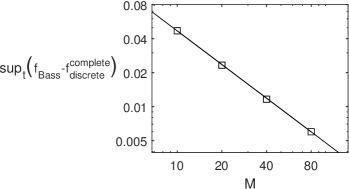
Figure 1. Log-log plot of $\sup_{t}\left(f_{\rm Bass}-f_{\rm discrete}^{\rm complete}\right)$ as a function of $M$. The fitted solid line is $\log y=-0.99\log M-0.78$. Here, $p=0.02$ and $q=0.1$.

3.1. Convergence and rate of convergence

The proof of Theorem 2 makes use of

Lemma 2.

For any $n\in\mathbb{N}$ and $p,q>0$, the solution $[S^{n}](t;p,q,M)$ of (14) converges, uniformly in $t$, to the solution $[S^{n}_{\infty}](t;p,q)$ of (16) as $M\to\infty$. Moreover, $[S^{n}](t;M)-[S^{n}_{\infty}](t)=O\left(\frac{1}{M}\right)$ as $M\to\infty$.

This lemma will be proved in Corollary 1 below. To simplify the notations, let

$$u^{(M)}_{n}(t):=[S^{n}](t;M),\qquad q^{(M)}_{n}:=\frac{M-n}{M-1}q,\qquad n=1,\dots,M,$$ (20a)

$$u^{\infty}_{n}(t):=[S^{n}_{\infty}](t),\qquad n=1,2,\dots,$$ (20b)

Then we can rewrite the systems (14) and (16) as

$$\frac{d}{dt}u^{(M)}_{n}(t)=-n\left(p+q^{(M)}_{n}\right)u^{(M)}_{n}+nq^{(M)}_{n}u^{(M)}_{n+1}.\qquad u^{(M)}_{n}(0)=1,\qquad n=1,\dots,M,$$ (21)

and

$$\frac{d}{dt}{u}_{n}^{\infty}(t)=-n(p+q)u_{n}^{\infty}+nqu_{n+1}^{\infty},\qquad u_{n}^{\infty}(0)=1,\qquad n=1,2,\dots,$$ (22)

respectively. Note that ODE (21) for $\frac{d}{dt}u^{(M)}_{M}$ does not involve the non-existent variable $u^{(M)}_{M+1}$, since

$$q_{M}^{(M)}=0.$$ (23)

For any fixed $n$,

$$\lim_{M\to\infty}q^{(M)}_{n}=q.$$ (24)

Hence, it is reasonable to expect that as $M\to\infty$, solutions of (21) converge to solutions of the limiting infinite system (22). We cannot, however, prove this by applying the standard theorems for continuous dependence of ODE solutions on parameters, since the number of equations increases with $M$ and becomes infinite in the limit, and because of the presence of the unbounded factor $n$ on the right-hand-sides of (21) and (22).

It is convenient for the analysis to have an infinite number of ODEs even for a finite $M$, because then $\{u_{n}^{(M)}\}$ and $\{u_{n}^{\infty}\}$ belong to the same space. Therefore, we embed the finite system (21) into the infinite system

$$\frac{d}{dt}u^{(M)}_{n}(t)=-n\left(p+q^{(M)}_{n}\right)u^{(M)}_{n}+nq^{(M)}_{n}u^{(M)}_{n+1},\qquad u^{(M)}_{n}(0)=1,\qquad n=1,2,\dots,$$ (25a)

where

$$q^{(M)}_{n}=\begin{cases}\frac{M-n}{M-1}q,&\quad n=1,\dots,M,\\ q,&\quad n=M+1,M+2,\dots\end{cases}$$ (25b)

Condition (23) ensures that the first $M$ components $\{u^{(M)}_{n}\}_{n=1}^{M}$ of the solution of (25) are also the solution of (21). In addition, $u^{(M)}_{n}=u_{n}^{\infty}$ for $n=M+1,M+2,\dots$, since equations (22) and (25) for these components are identical, and are decoupled from the first $M$ equations. Hence, solutions of the finite system (21) converge to solutions of the limiting infinite system (22) if and only if solutions of the infinite system (25) converge to that limit.

The discussion so far takes for granted that solutions of the infinite systems (22) and (25) exist. Even though those systems are linear, the existence of solutions is not quite trivial, because the presence of the factor $n$ on the right-hand-sides of (25a) and (22) makes those right-hand-sides unbounded functions of the infinite solution vectors

$$\mathbf{u}^{\infty}\mathrel{:=}(u_{1}^{\infty},u_{2}^{\infty},\cdots),\qquad\mathbf{u}^{(M)}\mathrel{:=}(u_{1}^{(M)},u_{2}^{(M)},\cdots).$$ (26)

From the proof of Theorem 2, however, it follows that

$$u_{n}^{\infty} =(1-f_{\rm Bass})^{n},\qquad n=1,2,\dots,$$

$$u_{n}^{(M)} =(1-f_{\rm Bass})^{n},\qquad n=M+1,M+2,\dots.$$ (27)

Therefore, solutions of the infinite systems (22) and (25) do exist.

The following technical results will be used in the statement and proof of Theorem 3.

Lemma 3.

Let $p,q>0$, let $q^{(M)}_{n}$ be given by (25b), and let

$$\widetilde{\epsilon}\mathrel{:=}\ln(1+\tfrac{p}{q}).$$ (28)

In addition, for every $\epsilon\geq 0$ and ${\bf v}=(v_{1},v_{2},\dots)\in{\mathbb{R}}^{\mathbb{N}}$, define

$$\theta(\epsilon)\mathrel{:=}\frac{qe^{\epsilon}}{p+q},\qquad\|\mathbf{v}\|_{\epsilon}\mathrel{:=}\sup_{1\leq n<\infty}e^{-\epsilon n}|v_{n}|,\qquad{\left|\mkern-1.5mu\left|\mkern-1.5mu\left|\mathbf{v}\right|\mkern-1.5mu\right|\mkern-1.5mu\right|}_{\epsilon}\mathrel{:=}\sup_{t\geq 0}\|\mathbf{v}(t)\|_{\epsilon}.$$ (29)

Then

$$\theta(\epsilon)<1,\qquad 0\leq\epsilon<\widetilde{\epsilon}.$$ (30)

In addition, the function $\|{\bf v}\|_{\epsilon}$ is a norm on the space ${\bf V}_{\epsilon}:=\{{\bf v}\,\Huge|\,\|{\bf v}\|_{\epsilon}<\infty\},$ and the function ${\left|\mkern-1.5mu\left|\mkern-1.5mu\left|{\bf v}(t)\right|\mkern-1.5mu\right|\mkern-1.5mu\right|}_{\epsilon}$ is a norm on the space $C^{0}_{B}([0,\infty),{\bf V}_{\epsilon})$ of bounded continuous functions on $[0,\infty)$ taking values in ${\bf V}_{\epsilon}$.

Proof.

These are standard results. ∎

Theorem 3.

Let $p,q>0$ and $0<\epsilon<\widetilde{\epsilon}$. Let ${\mathbf{u}}^{\infty}$ and ${\mathbf{u}}^{(M)}$ be the solutions of (22) and (25), respectively. Then

$${\left|\mkern-1.5mu\left|\mkern-1.5mu\left|\mathbf{u}^{(M)}-{\mathbf{u}}^{\infty}\right|\mkern-1.5mu\right|\mkern-1.5mu\right|}_{\epsilon}=O\left(\frac{1}{M}\right),\qquad M\to\infty.$$ (31)

Proof.

Since $\{u^{(M)}_{n}\}_{n=1}^{M}$ are probabilities, see (20a), they are bounded between 0 and 1. In addition, $\{u^{(M)}_{n}\}_{n=M+1}^{\infty}$ are given by (27), and so are also bounded between 0 and 1. Therefore, we have the uniform bound

$${\left|\mkern-1.5mu\left|\mkern-1.5mu\left|{\mathbf{u}}^{(M)}\right|\mkern-1.5mu\right|\mkern-1.5mu\right|}_{0}\leq 1.$$ (32)

Both here and in the other cases presented in this paper, the slighty weaker uniform bound ${\left|\mkern-1.5mu\left|\mkern-1.5mu\left|\mathbf{u}^{(M)}\right|\mkern-1.5mu\right|\mkern-1.5mu\right|}_{0}\leq\frac{1}{1-\theta(0)}$ can be obtained directly from relevant system, in this case  (25), by multiplying by an integrating factor, integrating, applying the ${\left|\mkern-1.5mu\left|\mkern-1.5mu\left|\,\right|\mkern-1.5mu\right|\mkern-1.5mu\right|}_{0}$ norm, and estimating the result, in similar fashion to the calculation below.

Subtracting (22) from (25) yields

$$\frac{d}{dt}\left(u^{(M)}_{n}-u_{n}^{\infty}\right) +n(p+q)\left(u^{(M)}_{n}-u_{n}^{\infty}\right)$$

$$\qquad=nq\left(u^{(M)}_{n+1}-u_{n+1}^{\infty}\right)+n\left(q-q^{(M)}_{n}\right)\left(u^{(M)}_{n}-u^{(M)}_{n+1}\right).$$

Multiplying by the integrating factor $e^{n(p+q)t}$, integrating from zero to $t$, and using $u^{(M)}_{n}(0)=u_{n}^{\infty}(0)$, yields

$$u^{(M)}_{n}(t)-u_{n}^{\infty}(t) =nq\int_{0}^{t}e^{-n(p+q)(t-s)}\left(u^{(M)}_{n+1}(s)-u_{n+1}^{\infty}(s)\right)\,ds$$ (33)

$$\qquad+n\left(q-q^{(M)}_{n}\right)\int_{0}^{t}e^{-n(p+q)(t-s)}\left(u^{(M)}_{n}(s)-u^{(M)}_{n+1}(s)\right)\,ds.$$

Let $0<\epsilon<\widetilde{\epsilon}$. Multiplying both sides of the infinite system (33) by $e^{-n\epsilon}$, and taking the supremum over $n,t$ gives

$${\left|\mkern-1.5mu\left|\mkern-1.5mu\left|\mathbf{u}^{(M)}-\mathbf{u}^{\infty}\right|\mkern-1.5mu\right|\mkern-1.5mu\right|}_{\epsilon}\leq\sup_{t,n}e^{\epsilon}nq\int_{0}^{t}e^{-n(p+q)(t-s)}{\left|\mkern-1.5mu\left|\mkern-1.5mu\left|\mathbf{u}^{(M)}-\mathbf{u}^{\infty}\right|\mkern-1.5mu\right|\mkern-1.5mu\right|}_{\epsilon}\,ds$$

$$\qquad\qquad\qquad\qquad+\sup_{t,n}e^{-n\epsilon}n\left|q-q^{(M)}_{n}\right|\int_{0}^{t}e^{-n(p+q)(t-s)}2{\left|\mkern-1.5mu\left|\mkern-1.5mu\left|\mathbf{u}^{(M)}\right|\mkern-1.5mu\right|\mkern-1.5mu\right|}_{0}\,ds$$

$$\quad=\sup_{t,n}\frac{qe^{\epsilon}(1-e^{-n(p+q)t})}{p+q}{\left|\mkern-1.5mu\left|\mkern-1.5mu\left|\mathbf{u}^{(M)}-\mathbf{u}^{\infty}\right|\mkern-1.5mu\right|\mkern-1.5mu\right|}_{\epsilon}$$

$$\qquad\qquad+2{\left|\mkern-1.5mu\left|\mkern-1.5mu\left|\mathbf{u}^{(M)}\right|\mkern-1.5mu\right|\mkern-1.5mu\right|}_{0}\sup_{t,n}\frac{\left|q-q^{(M)}_{n}\right|e^{-n\epsilon}(1-e^{-n(p+q)t})}{p+q}$$

$$\quad\leq\theta(\epsilon){\left|\mkern-1.5mu\left|\mkern-1.5mu\left|\mathbf{u}^{(M)}-\mathbf{u}^{\infty}\right|\mkern-1.5mu\right|\mkern-1.5mu\right|}_{\epsilon}+2\frac{\sup_{n}\left(\left|q-q^{(M)}_{n}\right|e^{-n\epsilon}\right)}{p+q},$$

where in the last inequality we used (32). Since $\theta(\epsilon)<1$, see (30), then

$${\left|\mkern-1.5mu\left|\mkern-1.5mu\left|\mathbf{u}^{(M)}-\mathbf{u}^{\infty}\right|\mkern-1.5mu\right|\mkern-1.5mu\right|}_{\epsilon}\leq\frac{2}{(p+q)(1-\theta(\epsilon))}\sup_{n}\left(\left|q-q^{(M)}_{n}\right|e^{-n\epsilon}\right).$$ (34)

By the definition of $q^{(M)}_{n}$, see (25b), for any $n\geq 1$,

$$\left|q-q^{(M)}_{n}\right|e^{-n\epsilon}\leq q\frac{n-1}{M-1}e^{-n\epsilon}\leq\frac{q}{\epsilon(M-1)}\left(n\epsilon e^{-n\epsilon}\right)\leq\frac{q}{\epsilon(M-1)}C,$$

where $C:=\max_{y\geq 0}(ye^{-y})<\infty$. Therefore, for any fixed $\epsilon>0$,

$$\sup_{n}\left(\left|q-q^{(M)}_{n}\right|e^{-n\epsilon}\right)=O\left(\frac{1}{M}\right),\qquad M\to\infty.$$ (35)

Relation (31) follows from (34) and (35). ∎

Corollary 1.

for any $n\in\mathbb{N}$, $u^{(M)}_{n}(t)\to u_{n}^{\infty}(t)$ uniformly in $t$ as $M\to\infty$, and $u^{(M)}_{n}(t)-u_{n}^{\infty}(t)=O\left(\frac{1}{M}\right)$ as $M\to\infty$.

Proof.

For any $n\in\mathbb{N}$ and $0<\epsilon<\tilde{\epsilon}$.

$$\left|u^{(M)}_{n}(t)-u_{n}^{\infty}(t)\right|\leq e^{n\epsilon}{\left|\mkern-1.5mu\left|\mkern-1.5mu\left|\mathbf{u}^{(M)}-\mathbf{u}^{\infty}\right|\mkern-1.5mu\right|\mkern-1.5mu\right|}_{\epsilon},$$ (36)

see (29). Therefore, the result follows from the convergence estimate (31). ∎

4. Homogeneous circle

To understand the role of the network in the discrete Bass model, it is instructive to consider the diffusion on the “opposite of a complete network”, namely, on a circle with $M$ nodes, where each node has only 2 edges. Thus, we assume that

$$p_{j}\equiv p,\qquad d_{j}(M)\equiv 2,\qquad q_{i,j}=\begin{cases}{q},&i=j\pm 1\mod M,\\ 0,&{\rm otherwise,}\end{cases},\qquad 1\leq i,j\leq M.$$ (37)

In this case, (4) reads

$${}{\rm Prob}(X_{j}(t+\Delta t)=1\ |\ {\bf X}(t))=\begin{cases}\hfill 1,\hfill&\qquad{\rm if}\ X_{j}(t)=1,\\ \left(p+\frac{q}{2}X_{j-1}(t)+\frac{q}{2}X_{j+1}(t)\right)\Delta t,&\qquad{\rm if}\ X_{j}(t)=0.\end{cases}$$ (38)

The $M\to\infty$ limit of the discrete Bass model on a circle was explicitly computed by Fibich and Gibori:

Theorem 4 ([13]).

The expected fraction of adopters in the discrete Bass model $(\ref{eq:general_initial},\ref{eq:general_circle})$ on a homogeneous circle as $M\to\infty$ is

$$\lim\limits_{M\to\infty}f^{\rm circle}_{\rm discrete}(t;p,q,M)=f_{\rm 1D}(t;p,q),\qquad f_{\rm 1D}(t;p,q):=1-e^{-(p+q)t+q\frac{1-e^{-pt}}{p}}.$$ (39)

Proof.

We sketch the proof of [13]. Let $[S^{n}_{\rm circle}](t)$ denote the probability that $n$ adjacent nodes $[S_{k+1},\dots,S_{k+n}]$ are all nonadopters at time $t$. By translation invariance, $[S_{k+1},\dots,S_{k+n}]$ is independent of $k$. Hence,

$$f^{\rm circle}_{\rm discrete}=1-[S^{1}_{\rm circle}].$$

By translation invariance and (37), the master equations (6) reduce to

$$\frac{d}{dt}[S^{n}_{\rm circle}] =-(np+q)[S^{n}_{\rm circle}]+q[S^{n+1}_{\rm circle}],\qquad n=1,\dots,M-1,$$ (40a)

$$\frac{d}{dt}[S^{M}_{\rm circle}] =-Mp[S^{M}_{\rm circle}],$$ (40b)

subject to the initial conditions

$$[S^{n}_{\rm circle}](0)=1\qquad n=1,\dots,M.$$ (40c)

Fixing $n$ and letting $M\to\infty$ in (40) gives the limiting system

$$\frac{d}{dt}[S^{n}_{\infty,\rm circle}]=-(np+q)[S^{n}_{\infty,\rm circle}]+q[S^{n+1}_{\infty,\rm circle}],\qquad[S^{n}_{\infty,\rm circle}](0)=1,\qquad n=1,2,\dots$$ (41)

The ansatz

$$[S^{n}_{\infty,\rm circle}]=e^{-(n-1)pt}[S_{\infty,\rm circle}]$$ (42)

reduces (41) into the single ODE

$$\frac{d}{dt}[S_{\infty,\rm circle}]=-(p+q)[S_{\infty,\rm circle}]+qe^{-pt}[S_{\infty,\rm circle}],\qquad[S_{\infty,\rm circle}](0)=1.$$

Hence

$$[S_{\infty,\rm circle}]=e^{-(p+q)t+q\frac{1-e^{-pt}}{p}}.$$

Since $\lim\limits_{M\to\infty}f^{\rm circle}_{\rm discrete}(t;p,q,M)=1-[S_{\infty,\rm circle}]$, the result follows.

Note, however, that in [13], Fibich and Gibori did not rigorously justify that (41) is the limit of (40) as $M\to\infty$. We will justify this limit, and thus complete the proof of Theorem 4, in Section 4.1. ∎

4.1. Convergence and rate of convergence

Theorem 5.

Assume the conditions of Theorem 4. Then the limit (39) is uniform in $t$. Moreover, the rate of convergence is exponential, i.e., for any $0<\epsilon<\widetilde{\epsilon}$, where $\widetilde{\epsilon}$ is given by (28),

$$f^{\rm circle}_{\rm discrete}(t;p,q,M)-f_{\rm 1D}(t;p,q)=O\left(e^{-M\epsilon}\right),\qquad M\to\infty.$$ (43)

Proof.

In light of the proof of Theorem 4, it only remains to show that for any $n\in\mathbb{N}$ and $p,q>0$:

1. The solution $[S^{n}_{\rm circle}](t;p,q,M)$ of (40) converges, uniformly in $t$, to the solution $[S^{n}_{\infty,\rm circle}](t;p,q)$ of (41) as $M\to\infty$.

2. The rate of convergence is exponential, i.e.,

   $$[S^{n}_{\rm circle}](t;M)-[S^{n}_{\infty,\rm circle}](t)=O\left(e^{-M\epsilon}\right),\qquad M\to\infty.$$

These results are proved in Corollary 2 below. ∎

The exponential rate of convergence predicted in Theorem 5 is illustrated numerically in Figure 2, where we observe that $f_{\rm 1D}-f^{\rm circle}_{\rm discrete}\approx Ce^{-1.3M}$. Here $f^{\rm circle}_{\rm discrete}(t;p,q,M)$ was calculated using the explicit expression obtained in [13, 15].

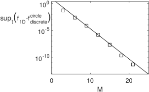
Figure 2. Semi-log plot of $\sup_{t}\left(f_{\rm 1D}-f^{\rm circle}_{\rm discrete}\right)$ as a function of $M$. The fitted solid line is $y=8.8e^{-1.3M}$. Here, $p=0.02$ and $q=0.11$.

The analysis that leads to Corollary 2 is nearly identical to that in Section 3.1, thus illustrating the power of our method. Let

$$u^{(M)}_{n}(t):=[S^{n}_{\rm circle}](t;M),\qquad q^{(M)}_{n}:=\begin{cases}q,&n=1,\dots,M-1,\\ 0,&n=M,\end{cases}\qquad n=1,\dots,M,$$ (44a)

$$u^{\infty}_{n}(t):=[S^{n}_{\infty,\rm circle}](t),\qquad n=1,2,\dots.$$ (44b)

Then we can rewrite the systems (40) and (41) as

$$\frac{d}{dt}u^{(M)}_{n}(t)=-\left(np+q^{(M)}_{n}\right)u^{(M)}_{n}+q^{(M)}_{n}u^{(M)}_{n+1}.\qquad u^{(M)}_{n}(0)=1,\qquad n=1,\dots,M,$$ (45)

and

$$\frac{d}{dt}{u}_{n}^{\infty}(t)=-(np+q)u_{n}^{\infty}+qu_{n+1}^{\infty},\qquad u_{n}^{\infty}(0)=1,\qquad n=1,2,\dots,$$ (46)

respectively. We embed (45) into the infinite system

$$\frac{d}{dt}u^{(M)}_{n}(t)=-\left(np+q^{(M)}_{n}\right)u^{(M)}_{n}+q^{(M)}_{n}u^{(M)}_{n+1},\qquad u^{(M)}_{n}(0)=1,\qquad n=1,2,\dots,$$ (47a)

where

$$q^{(M)}_{n}=\begin{cases}q,&\quad n\neq M,\\ 0,&\quad n=M.\end{cases}$$ (47b)

By (42),

$$u_{n}^{\infty} =e^{-(n-1)pt}[S_{\infty,\rm circle}],\qquad n=1,2,\dots,$$

$$u_{n}^{(M)} =e^{-(n-1)pt}[S_{\infty,\rm circle}],\qquad n=M+1,M+2,\dots.$$ (48)

Therefore, solutions of the infinite systems (46) and (47) do exist.

Lemma 4.

Let $p,q>0$ and $0<\epsilon<\widetilde{\epsilon}$, where $\widetilde{\epsilon}$ is given by (28). Let ${\mathbf{u}}^{\infty}$ and ${\mathbf{u}}^{(M)}$ be the solutions of (46) and (47), respectively. Then

$${\left|\mkern-1.5mu\left|\mkern-1.5mu\left|\mathbf{u}^{(M)}-{\mathbf{u}}^{\infty}\right|\mkern-1.5mu\right|\mkern-1.5mu\right|}_{\epsilon}=O\left(e^{-M\epsilon}\right),\qquad M\to\infty.$$ (49)

Proof.

Since $\{u^{(M)}_{n}\}_{n=1}^{M}$ are probabilities, see (44a), they are bounded between 0 and 1. In addition, $\{u^{(M)}_{n}\}_{n=M+1}^{\infty}$ are given by (48), and so are also bounded between 0 and 1. Therefore, we have the uniform bound

$${\left|\mkern-1.5mu\left|\mkern-1.5mu\left|{\mathbf{u}}^{(M)}\right|\mkern-1.5mu\right|\mkern-1.5mu\right|}_{0}\leq 1.$$ (50)

Subtracting (46) from (45) yields

$$\frac{d}{dt}\left(u^{(M)}_{n}-u_{n}^{\infty}\right) +(np+q)\left(u^{(M)}_{n}-u_{n}^{\infty}\right)$$

$$\qquad=q\left(u^{(M)}_{n+1}-u_{n+1}^{\infty}\right)+\left(q-q^{(M)}_{n}\right)\left(u^{(M)}_{n}-u^{(M)}_{n+1}\right).$$

Multiplying by the integrating factor $e^{(np+q)t}$, integrating from zero to $t$, and using $u^{(M)}_{n}(0)=u_{n}^{\infty}(0)$, yields

$$u^{(M)}_{n}(t)-u_{n}^{\infty}(t) =q\int_{0}^{t}e^{-(np+q)(t-s)}\left(u^{(M)}_{n+1}(s)-u_{n+1}^{\infty}(s)\right)\,ds$$ (51)

$$\qquad+\left(q-q^{(M)}_{n}\right)\int_{0}^{t}e^{-(np+q)(t-s)}\left(u^{(M)}_{n}(s)-u^{(M)}_{n+1}(s)\right)\,ds.$$

Let $0<\epsilon<\widetilde{\epsilon}$. Multiplying both sides of the infinite system (51) by $e^{-n\epsilon}$, and taking the supremum over $n,t$ gives

$${\left|\mkern-1.5mu\left|\mkern-1.5mu\left|\mathbf{u}^{(M)}-\mathbf{u}^{\infty}\right|\mkern-1.5mu\right|\mkern-1.5mu\right|}_{\epsilon}\leq\sup_{t,n}e^{\epsilon}q\int_{0}^{t}e^{-(np+q)(t-s)}{\left|\mkern-1.5mu\left|\mkern-1.5mu\left|\mathbf{u}^{(M)}-\mathbf{u}^{\infty}\right|\mkern-1.5mu\right|\mkern-1.5mu\right|}_{\epsilon}\,ds$$

$$\qquad\qquad\qquad\qquad+\sup_{t,n}e^{-n\epsilon}\left|q-q^{(M)}_{n}\right|\int_{0}^{t}e^{-(np+q)(t-s)}2{\left|\mkern-1.5mu\left|\mkern-1.5mu\left|\mathbf{u}^{(M)}\right|\mkern-1.5mu\right|\mkern-1.5mu\right|}_{0}\,ds$$

$$\quad=\sup_{t,n}\frac{qe^{\epsilon}(1-e^{-(np+q)t})}{np+q}{\left|\mkern-1.5mu\left|\mkern-1.5mu\left|\mathbf{u}^{(M)}-\mathbf{u}^{\infty}\right|\mkern-1.5mu\right|\mkern-1.5mu\right|}_{\epsilon}$$

$$\qquad\qquad+2{\left|\mkern-1.5mu\left|\mkern-1.5mu\left|\mathbf{u}^{(M)}\right|\mkern-1.5mu\right|\mkern-1.5mu\right|}_{0}\sup_{t,n}\frac{\left|q-q^{(M)}_{n}\right|e^{-n\epsilon}(1-e^{-(np+q)t})}{np+q}$$

$$\quad\leq\theta(\epsilon){\left|\mkern-1.5mu\left|\mkern-1.5mu\left|\mathbf{u}^{(M)}-\mathbf{u}^{\infty}\right|\mkern-1.5mu\right|\mkern-1.5mu\right|}_{\epsilon}+2\frac{\sup_{n}\left(\left|q-q^{(M)}_{n}\right|e^{-n\epsilon}\right)}{p+q},$$

where in the last inequality we used (50). Since $\theta(\epsilon)<1$, see (30), then

$${\left|\mkern-1.5mu\left|\mkern-1.5mu\left|\mathbf{u}^{(M)}-\mathbf{u}^{\infty}\right|\mkern-1.5mu\right|\mkern-1.5mu\right|}_{\epsilon}\leq\frac{2}{(p+q)(1-\theta(\epsilon))}\sup_{n}\left(\left|q-q^{(M)}_{n}\right|e^{-n\epsilon}\right).$$ (52)

By the definition of $q^{(M)}_{n}$, see (47b),

$$\sup_{n}\left(\left|q-q^{(M)}_{n}\right|e^{-n\epsilon}\right)=\left|q-q^{(M)}_{M}\right|e^{-M\epsilon}=qe^{-M\epsilon}.$$ (53)

Relation (49) follows from (52) and (53). ∎

Corollary 2.

For any $n\in\mathbb{N}$ and $0<\epsilon<\tilde{\epsilon}$, $u^{(M)}_{n}(t)\to u_{n}^{\infty}(t)$ uniformly in $t$ as $M\to\infty$, and $u^{(M)}_{n}(t)-u_{n}^{\infty}(t)=O\left(e^{-M\epsilon}\right)$ as $M\to\infty$.

Proof.

Same as Corollary 1, only with the convergence estimate (49). ∎

5. Heterogeneous network with $K$ homogeneous groups

We now consider a heterogeneous population that consists of $K$ groups, each of which is homogeneous. This situation arises, e.g., when we divide the population according to age groups, levels of income, gender, etc.

5.1. Description of the model

The network consists of $K$ groups. Any node in group $k$ has external influence $p_{k}>0$, any adopter in group $m$ has internal influence $\frac{q_{m,k}}{M-1}\geq 0$ on any nonadopter in group $k$, and the parameters $\{p_{j}\}$ and $\{q_{m,j}\}$ are assumed to satisfy

$$p_{j}>0,\quad q_{m,j}\geq 0\qquad\text{for $m,j\in\{1,\cdots,K\}$.}$$ (54)

Group $k$ has $M_{k}>0$ nodes, and so $\sum_{k=1}^{K}M_{k}=M$.

The discrete model (4) for node $k_{n}$ in group $k$, where $k=1,\dots,K$ and $n=1,\dots,M_{k}$, becomes

$${\rm Prob}(X_{k_{n}}(t+\Delta t)=1\ |\ {\bf X}(t))=\begin{cases}\hfill 1,\hfill&\qquad{\rm if}\ X_{k_{n}}(t)=1,\\ \left(p_{k}+\sum\limits_{m=1}^{K}\frac{q_{m,k}}{M-1}N_{m}(t)\right)\Delta t,&\qquad{\rm if}\ X_{k_{n}}(t)=0,\end{cases}$$ (55)

where $N_{m}(t)$ is the number of adopters in group $m$. The corresponding heterogeneous compartmental Bass model reads, cf. (1),

$$\frac{d}{dt}n_{k}(t)=(M_{k}-n_{k})\left(p_{k}+\sum_{m=1}^{K}\frac{q_{m,k}}{M}n_{m}\right),\qquad n_{k}(0)=0,\qquad 1\leq k\leq K,$$ (56)

where $n_{k}$ is the number of adopters in group $k$. Although complete consistency with (55) would require dividing $q_{m,k}$ in (56) by $M-1$ rather than $M$, the use of $M$ as the denominator is traditional in Bass models, going back to Bass [5]. In any case, the difference becomes $O\left(\frac{1}{M}\right)$ as $M\to\infty$.

Let us assume that the following limits exist and are positive:

$$a_{k}:=\lim\limits_{M\to\infty}\frac{M_{k}}{M},\qquad k=1,\ldots,K.$$ (57)

Then $a_{k}>0$ and $\sum_{k=1}^{K}a_{k}=1$. Moreover, we assume that

$$\frac{M_{k}}{M}-a_{k}=O\left(\frac{1}{M}\right)\qquad\text{as }M\to\infty,\qquad 1\leq k\leq K.$$ (58)

Relation (58) holds trivially when $K=1$. For $K\geq 2$, it holds if, e.g., $M_{k}=\lfloor a_{k}M\rfloor$ for $1\leq k\leq K-1$ and $M_{K}=M-\sum_{k=1}^{K-1}M_{k}$.

Let $f_{k}:=\frac{n_{k}}{M}$ denote the fraction within the population of group-$k$ adopters. Then (56) can be rewritten as

$$\frac{d}{dt}f_{k}(t)=(\tfrac{M_{k}}{M}-f_{k})\left(p_{k}+\sum_{m=1}^{K}q_{m,k}f_{m}\right),\qquad f_{k}(0)=0,\qquad 1\leq k\leq K.$$ (59)

Since the number of equations in (59) remains fixed as $M\to\infty$, assumption (57), together with standard results on the continuous dependence of solutions of systems of ODEs on parameters and the fact that $f_{k}$ tends to the constant value $\frac{M_{k}}{M}$ as $t\to\infty$, imply that the solution of (59) tends uniformly in time as $M$ tends to infinity to the solution of

$$\frac{d}{dt}f_{k}(t)=(a_{k}-f_{k})\left(p_{k}+\sum_{m=1}^{K}q_{m,k}f_{m}\right),\qquad f_{k}(0)=0,\qquad 1\leq k\leq K,$$ (60)

and assumption (58) implies that the rate of convergence is $O(\frac{1}{M})$.

When $K=1$, both (59) and (60) reduce to (8). Since the solution $f_{k}$ of (60) satisfies $0\leq f_{k}\leq a_{k}$, the maximal influence on a nonadopter from group $k$ is, c.f. (3),

$$q_{k}:=\sum_{m=1}^{K}a_{m}q_{m,k}.$$ (61)

5.2. Convergence and rate of convergence

We can use our method to prove the convergence and the rate of convergence of the $K$-groups heterogeneous discrete Bass model to the heterogeneous compartmental Bass model.

Theorem 6.

Let (54) and (58) hold. Then the expected fraction of adopters in the discrete Bass model $(\ref{eq:general_initial},\ref{eq:discrete_group_model})$ on a heterogeneous network with $K$ groups approaches that of the corresponding heterogeneous compartmental Bass model (60) as $M\to\infty$, i.e.,

$$\lim\limits_{M\to\infty}f^{\rm heter}_{\rm discrete}(t;\{p_{k}\},\{q_{i,k}\},\{a_{k}\},M)=f^{\rm heter}_{\rm Bass}(t;\{p_{k}\},\{q_{i,k}\},\{a_{k}\}),$$ (62)

where $f^{\rm heter}_{\rm Bass}:=\sum_{k=1}^{K}f_{k}$, $\{f_{k}\}$ are the solutions of (60), and the limit is uniform in $t$. Moreover, the rate of convergence is $\frac{1}{M}$, i.e.,

$$f^{\rm heter}_{\rm Bass}(t)-f^{\rm heter}_{\rm discrete}(t)=O\left(\frac{1}{M}\right),\qquad M\to\infty.$$ (63)

Proof.

Let $\vec{M}:=\left(M_{1},\ldots,M_{K}\right)^{T}$, $\vec{k}:=(k_{1},\cdots,k_{K})^{T}$,

$$n(\vec{k}):=\sum_{j=1}^{K}k_{j},$$ (64)

and

$$\vec{K}^{\vec{M}}:=\{\vec{k}\ |\ k_{j}\in\{0,\dots,M_{j}\},\quad 1\leq n(\vec{k})\leq M\}.$$

Let $u_{\vec{k}}(t)$ denote the probability that a set $\{m_{1},\dots,m_{n}\}$ of $n=n(\vec{k})$ consumers which contains $k_{j}$ members from group $j$ for $1\leq j\leq K$, are all non-adopters at time $t$. The master equations (6) reduce to

$$\tfrac{d\hfill}{dt}u_{\vec{k}}(t)=-\left(\vec{k}\cdot\vec{p}+\frac{\left(\vec{M}-\vec{k}\right)}{M-1}^{T}Q{\vec{k}}\right)u_{\vec{k}}+\frac{\left(\vec{M}-\vec{k}\right)}{M-1}^{T}D\left(u_{\vec{k}+\vec{e}_{1}},\cdots,u_{\vec{k}+\vec{e}_{K}}\right)Q{\vec{k}},$$ (65a)

for $$1\leq n(\vec{k})\leq M-1$$, and

$$\tfrac{d\hfill}{dt}u_{\vec{M}}(t)=-\left(\vec{M}\cdot\vec{p}\right)u_{\vec{M}},$$ (65b)

subject to

$$u_{\vec{k}}(0)=1,\qquad\vec{k}\in\vec{K}^{\vec{M}},$$ (65c)

where $$\vec{e}_{i} i$$ is the unit vector in the th coordinate,

$$Q=\left(q_{i,j}\right)=\begin{pmatrix}q_{1,1}&\cdots&q_{1,K}\\ \vdots&\ddots&\vdots\\ q_{K,1}&\cdots&q_{K,K}\end{pmatrix},\qquad D\left(\lambda_{1},\cdots,\lambda_{n}\right)=\begin{pmatrix}\lambda_{1}&&\text{\large$0$}\\ &\ddots\\ \text{\large$0$}&&\lambda_{n}\end{pmatrix}.$$

If we formally fix $\vec{k}$, let $M\to\infty$ in (65), and use (57), we get that

$$\tfrac{d\hfill}{dt}u_{\vec{k}}^{(\infty)}=-\left(\vec{k}\cdot\vec{p}+\vec{a}^{T}Q{\vec{k}}\right)u_{\vec{k}}^{(\infty)}+\vec{a}^{T}D\left(u_{\vec{k}+\vec{e}_{1}}^{(\infty)},\cdots,u_{\vec{k}+\vec{e}_{K}}^{(\infty)}\right)Q{\vec{k}},\qquad u_{\vec{k}}^{(\infty)}(0)=1,$$ (66)

where $\vec{a}:=\left(a_{1},\ldots,a_{K}\right)^{T}$. This does not immediately imply that

$$\lim_{M\to\infty}u_{\vec{k}}=u_{\vec{k}}^{(\infty)},$$ (67)

since the number of ODEs in (65) increases with $M$, and becomes infinite in the limit. In Lemma 5 below, however, we will prove that the limit (67) holds for any $\vec{k}\in\vec{K}^{\infty}$, where

$$\vec{K}^{\infty}:=\{\vec{k}\ |\ k_{j}\in\{0,1,2,\dots\},\quad 1\leq n(\vec{k})<\infty\}.$$

Therefore, we can proceed to solve the infinite system (66).

Let

$$u_{\vec{k}}^{(\infty)}(t):=\prod_{j=1}^{K}\left({u_{\vec{e}_{j}}^{(\infty)}}(t)\right)^{k_{j}},$$ (68a)

where

$$\tfrac{d\hfill}{dt}u_{\vec{e}_{j}}^{(\infty)}(t)=-\left(p_{j}+\sum_{i=1}^{K}a_{i}q_{i,j}\left(1-u_{\vec{e}_{i}}^{(\infty)}\right)\right)u_{\vec{e}_{j}}^{(\infty)},\qquad u_{\vec{e}_{j}}^{(\infty)}(0)=1,\quad j=1,\dots,K.$$ (68b)

It can be verified by direct substitution that (68) satisfies (66) for any $\vec{k}\in\vec{K}^{\infty}$.

Let

$$f_{j}:=a_{j}\left(1-u_{\vec{e}_{j}}^{(\infty)}\right),\qquad j=1,\dots,K.$$

By (68b), $\{f_{j}\}_{j=1}^{K}$ satisfy the heterogeneous compartmental Bass model (60). Hence,

$$\sum_{k=1}^{K}a_{k}u_{\vec{e}_{k}}^{(\infty)}=\sum_{k=1}^{K}\left(a_{k}-f_{k}\right)=1-f^{\rm heter}_{\rm Bass}.$$ (69a)

In addition, by (5),

$$\sum_{k=1}^{K}\frac{M_{k}}{M}u_{\vec{e}_{k}}=\frac{1}{M}\sum_{k=1}^{M}[S_{k}]=1-f^{\rm heter}_{\rm discrete}.$$ (69b)

Therefore, (62) and (63) follow from (69), (58), and Lemma 5. ∎

The $O\left(\frac{1}{M}\right)$ rate of convergence predicted in Theorem 6 is illustrated numerically in Figure 3, where we observe that $f^{\rm heter}_{\rm Bass}-f^{\rm heter}_{\rm discrete}\approx\frac{C}{M^{0.96}}$. Here $f^{\rm heter}_{\rm discrete}(t;\{p_{k}\},\{q_{m,k}\},M)$ was calculated from $10^{6}$ simulations of $(\ref{eq:general_initial},\ref{eq:discrete_group_model})$.

Figure 3. Log-log plot of $\sup_{t}\left(f^{\rm heter}_{\rm Bass}-f^{\rm heter}_{\rm discrete}\right)$ as a function of $M$. The fitted solid line is $\log y=-0.96\log M-0.58$. Here, $K=4$, $\{a_{1},a_{2},a_{3},a_{4}\}=\{0.4,0.1,0.3,0.2\}$, $\{p_{1},p_{2},p_{3},p_{4}\}=\{0,0.02,0.04,0.01\}$, and $\left(q_{i,j}\right)=\left(\begin{smallmatrix}0.1&0.05&0.01&0\\ 0.05&0.025&0.08&0.05\\ 0.01&0.02&0.03&0.04\\ 0.15&0.05&0.05&0.05\end{smallmatrix}\right)$ .

5.3. Proof of Lemma 5

As noted, the proof of Theorem 6 makes use of the following result:

Lemma 5.

For any $\vec{k}\in\vec{K}^{\infty}$, the solution $u_{\vec{k}}(t)$ of (65) converges, uniformly in $t$, to the solution $u_{\vec{k}}^{(\infty)}(t)$ of (66) as $M\to\infty$. Moreover,

$$u_{\vec{k}}-u_{\vec{k}}^{(\infty)}=O\left(\frac{1}{M}\right),\qquad M\to\infty.$$ (70)

This result is proved in Corollary 3 below.

Remark 6.

In some cases, it makes sense to replace (58) with a more general convergence rate

$$\frac{M_{k}}{M}-a_{k}=O\left(\frac{1}{M^{r}}\right)\qquad\text{as }M\to\infty,\qquad 1\leq k\leq K.$$ (71)

For example, if each person is assigned randomly to group $k$ with probability $a_{k}$ then large deviations theory together with the Borel-Cantelli lemma imply that estimate (71) holds almost surely for any $r<\frac{1}{2}$. In that case, the rate of convergence (63) and (70) changes from $1/M$ to $1/M^{\min(1,r)}$.

We now rigorously show that for any $\vec{k}\in\vec{K}^{\infty}$, the solution of (65) approaches the solution of (66) as $M\to\infty$. Similarly to the homogeneous case (Section 3.1), we first embed the finite system (65) into the infinite system

$$\tfrac{d\hfill}{dt}u_{\vec{k}}^{(\vec{M})}=-\left(\vec{k}\cdot\vec{p}+\vec{a}(\vec{M},\vec{k})Q\vec{k}\right)u_{\vec{k}}^{(\vec{M})}+\vec{a}(\vec{M},\vec{k})D \left(u_{\vec{k}+\vec{e}_{1}}^{(\vec{M})},\cdots,u_{\vec{k}+\vec{e}_{K}}^{(\vec{M})}\right)Q\vec{k},$$ (72a)

$$\quad u_{\vec{k}}^{(\vec{M})}(0)=1,\qquad\vec{k}\in\vec{K}^{\infty},$$

where

$$\vec{a}(\vec{M},\vec{k})\mathrel{:=}\begin{cases}\frac{\left(\vec{M}-\vec{k}\right)}{M-1}^{T},&\qquad\vec{k}\in\vec{K}^{\vec{M}},\\ \vec{a}^{T},&\qquad\vec{k}\in\vec{K}^{\infty}\backslash\vec{K}^{\vec{M}}.\end{cases}$$ (72b)

Thus, for $\vec{k}\in\vec{K}^{\vec{M}}$, the ODEs of the infinite systems (72) and (65) are identical. The ODEs of (72) for $\vec{k}\in\vec{K}^{\vec{M}}$ are decoupled from those for $\vec{k}\in\vec{K}^{\infty}\backslash\vec{K}^{\vec{M}}$, since $\vec{a}(\vec{M},\vec{k})(j)=0$ when $k_{j}=M_{j}$ for any $1\leq j\leq K$. In addition, the ODEs of the infinite systems (72) and (66) for $\vec{k}\in\vec{K}^{\infty}\backslash\vec{K}^{\vec{M}}$ are identical, and are decoupled from the corresponding ODEs for $\vec{K}^{\vec{M}}$. Therefore $u_{\vec{k}}^{(\vec{M})}\equiv u_{\vec{k}}^{(\infty)}$ for $\vec{k}\in\vec{K}^{\infty}\backslash\vec{K}^{\vec{M}}$. Hence, solutions of the finite system (65) converge to solutions of the limiting system (66) if and only if solutions of the infinite system (72) converge to that limit.

From the proof of Theorem 6, it follows that

$$u_{\vec{k}}^{(\infty)} =\prod_{j=1}^{K}(1-\frac{f_{j}}{a_{j}})^{k_{j}},\qquad\vec{k}\in\vec{K}^{\infty},$$

$$u_{\vec{k}}^{(\vec{M})} =\prod_{j=1}^{K}(1-\frac{f_{j}}{a_{j}})^{k_{j}},\qquad\vec{k}\in\vec{K}^{\infty}\backslash\vec{K}^{\vec{M}}.$$ (73)

Therefore, solutions of the infinite systems (66) and (72) do exist.

The following technical results will be used in the statement and proof of Theorem 7.

Lemma 7.

Let $\{p_{j}\}$ and $\{q_{m,j}\}$ satisfy (54), let $\vec{a}(\vec{M},\vec{k})$ be given by (72b), and let

$$A\mathrel{:=}\sup_{\vec{M}\in\mathbb{N}^{K},\vec{k}\in\vec{K}^{\infty},}\max_{\omega_{j}\geq 0,\sum_{j=1}^{K}\omega_{j}=1}\vec{a}(\vec{M},\vec{k})Q\vec{\omega},$$ (74)

where $\vec{\omega}=\left(\omega_{1},\dots,\omega_{K}\right)^{T}$ and $Q$ is defined in (65). Then $0<A<\infty$.

Define

$$\widetilde{\varepsilon}\mathrel{:=}\ln(1+\tfrac{\min_{j}p_{j}}{A}),\qquad\theta(\varepsilon)\mathrel{:=}\frac{Ae^{\varepsilon}}{\min_{j}p_{j}+A}.$$ (75)

Also, for every $\varepsilon\geq 0$ and $\mathbf{v}=\left(v_{1},v_{2},\dots\right)\in K^{\mathbb{N}}$, define

$$\|\mathbf{v}\|_{\varepsilon}\mathrel{:=}\sup_{\vec{k}\in\vec{K}^{\infty}}e^{-\varepsilon n(\vec{k})}|v_{\vec{k}}|,\qquad{\left|\mkern-1.5mu\left|\mkern-1.5mu\left|\mathbf{v}\right|\mkern-1.5mu\right|\mkern-1.5mu\right|}_{\varepsilon}\mathrel{:=}\sup_{t\geq 0}\|\mathbf{v}(t)\|,$$ (76)

where $n(\vec{k})$ is defined in (64). Then for all $0\leq\varepsilon<\widetilde{\varepsilon}$, $\vec{M}\in\mathbb{N}^{K}$, and $\vec{k}\in\vec{K}^{\infty}$,

$$\frac{\vec{a}(\vec{M},\vec{k})Q\vec{k}\,e^{\varepsilon}}{\vec{k}\cdot\vec{p}+\vec{a}(\vec{M},\vec{k})Q\vec{k}}\leq\theta(\varepsilon)<1.$$ (77)

In addition, the function $\|{\bf v}\|_{\varepsilon}$ is a norm on the space ${\bf V}_{\epsilon}:=\{{\bf v}\,\Huge|\,\|{\bf v}\|_{\epsilon}<\infty\},$ and the function ${\left|\mkern-1.5mu\left|\mkern-1.5mu\left|{\bf v}(t)\right|\mkern-1.5mu\right|\mkern-1.5mu\right|}_{\epsilon}$ is a norm on the space $C^{0}_{B}([0,\infty),{\bf V}_{\epsilon})$ of bounded continuous functions on $[0,\infty)$ taking values in ${\bf V}_{\epsilon}$.

Proof.

These are standard results. ∎

Theorem 7.

Assume the conditions of Lemma 7. Let ${\mathbf{u}}^{(\infty)}$ and ${\mathbf{u}}^{(M)}$ be the solutions of (66) and (72), respectively. Then for $0<\varepsilon<\widetilde{\varepsilon}$,

$${\big{|}\mkern-1.5mu\big{|}\mkern-1.5mu\big{|}\mathbf{u}^{(\vec{M})}-{\mathbf{u}}^{(\infty)}\big{|}\mkern-1.5mu\big{|}\mkern-1.5mu\big{|}}_{\varepsilon}=O\left(\frac{1}{M}\right),\qquad M\to\infty.$$ (78)

Proof.

Since $\{u^{(M)}_{\vec{k}}\}$ are probabilities for $\vec{k}\in\vec{K}^{\vec{M}}$, see (65), they are bounded between 0 and 1. In addition, $\{u^{(M)}_{\vec{k}}\}$ are given by (73) for $\vec{k}\in\vec{K}^{\infty}\backslash\vec{K}^{\vec{M}}$, and so are also bounded between 0 and 1. Therefore, we have the uniform bound

$${\left|\mkern-1.5mu\left|\mkern-1.5mu\left|{\mathbf{u}}^{(M)}\right|\mkern-1.5mu\right|\mkern-1.5mu\right|}_{0}\leq 1.$$ (79)

Subtracting (66) from (72) yields

$$\tfrac{d\hfill}{dt}\left[u^{(\vec{M})}_{\vec{k}}-u_{\vec{k}}^{(\infty)}\right] =-[\vec{k}\cdot\vec{p}+\vec{a}Q\vec{k}](u^{(\vec{M})}_{\vec{k}}-u_{\vec{k}}^{(\infty)})$$ (80)

$$\quad+\vec{a}D\left(u^{(\vec{M})}_{\vec{k}+\vec{e}_{1}}-u_{\vec{k}+\vec{e}_{1}}^{(\infty)},\cdots,u^{(\vec{M})}_{\vec{k}+\vec{e}_{K}}-u_{\vec{k}+\vec{e}_{K}}^{(\infty)}\right)Q\vec{k}$$

$$\quad+[\vec{a}-\vec{a}(\vec{M},\vec{k})]D\left(u^{(\vec{M})}_{\vec{k}}-u^{(\vec{M})}_{\vec{k}+\vec{e}_{1}},\cdots,u^{(\vec{M})}_{\vec{k}}-u^{(\vec{M})}_{\vec{k}+\vec{e}_{K}}\right)Q\vec{k}.$$

Multiplying by the integrating factor $e^{(\vec{k}\cdot\vec{p}+\vec{a}Q\vec{k})t}$, integrating from zero to $t$, and using $u^{(M)}_{\vec{k}}(0)=u_{\vec{k}}^{(\infty)}(0)$, yields

$$u^{(\vec{M})}_{\vec{k}}(t)-u_{\vec{k}}^{(\infty)}(t)$$ (81)

$$= \int_{0}^{t}e^{-(\vec{k}\cdot\vec{p}+\vec{a}Q\vec{k})(t-s)}\vec{a}D\left(u^{(\vec{M})}_{\vec{k}+\vec{e}_{1}}(s)-u_{\vec{k}+\vec{e}_{1}}^{(\infty)}(s),\cdots,u^{(\vec{M})}_{\vec{k}+\vec{e}_{K}}(s)-u_{\vec{k}+\vec{e}_{K}}^{(\infty)}(s)\right)Q\vec{k}\,ds$$

$$+ \int_{0}^{t}e^{-(\vec{k}\cdot\vec{p}+\vec{a}Q\vec{k})(t-s)}[\vec{a}-\vec{a}(\vec{M},\vec{k})]D\left(u^{(\vec{M})}_{\vec{k}}(s)-u^{(\vec{M})}_{\vec{k}+\vec{e}_{1}}(s),\cdots,u^{(\vec{M})}_{\vec{k}}(s)-u^{(\vec{M})}_{\vec{k}+\vec{e}_{K}}(s)\right)Q\vec{k}\,ds,$$

since $\mathbf{u}^{(\vec{M})}$ and $\mathbf{u}^{(\infty)}$ have the same initial data. Taking the ${\left|\mkern-1.5mu\left|\mkern-1.5mu\left|\,\right|\mkern-1.5mu\right|\mkern-1.5mu\right|}_{\varepsilon}$ norm with $0<\varepsilon<\widetilde{\varepsilon}$ of both sides of (81), estimating on the right, and using (79) yields

$${\big{|}\mkern-1.5mu\big{|}\mkern-1.5mu\big{|}\mathbf{u}^{(\vec{M})}-\mathbf{u}^{(\infty)}\big{|}\mkern-1.5mu\big{|}\mkern-1.5mu\big{|}}_{\varepsilon}$$ (82)

$$\quad\leq\sup_{t,\vec{k}}[\vec{a}Q\vec{k}]e^{-\varepsilon n(\vec{k})}\int_{0}^{t}e^{-(\vec{k}\cdot\vec{p}+\vec{a}Q\vec{k})(t-s)}e^{\varepsilon(1+n(\vec{k}))}{\big{|}\mkern-1.5mu\big{|}\mkern-1.5mu\big{|}\mathbf{u}^{(\vec{M})}-\mathbf{u}^{(\infty)}\big{|}\mkern-1.5mu\big{|}\mkern-1.5mu\big{|}}_{\varepsilon}\,ds$$

$$\qquad+\sup_{t,\vec{k}}2\sum_{i=1}^{K}\left|\vec{a}(\vec{M},\vec{k})(i)-a_{i}\right|\max_{i,j}q_{i,j}n(\vec{k})e^{-\varepsilon n(\vec{k})}\int_{0}^{t}e^{-(\vec{k}\cdot\vec{p}+\vec{a}Q\vec{k})(t-s)}{\big{|}\mkern-1.5mu\big{|}\mkern-1.5mu\big{|}\mathbf{u}^{(\vec{M})}\big{|}\mkern-1.5mu\big{|}\mkern-1.5mu\big{|}}_{0}\,ds$$

$$\quad=\sup_{t,\vec{k}}\frac{[\vec{a}Q\vec{k}]e^{\varepsilon}}{\vec{k}\cdot\vec{p}+\vec{a}Q\vec{k}}{\big{|}\mkern-1.5mu\big{|}\mkern-1.5mu\big{|}\mathbf{u}^{(M)}-\mathbf{u}^{(\infty)}\big{|}\mkern-1.5mu\big{|}\mkern-1.5mu\big{|}}_{\varepsilon}(1-e^{-(\vec{k}\cdot\vec{p}+\vec{a}Q\vec{k})t})$$

$$\qquad+\sup_{t,\vec{k}}\frac{2\sum_{i=1}^{K}\left|\vec{a}(\vec{M},\vec{k})(i)-a_{i}\right|\max_{i,j}q_{i,j}n(\vec{k})e^{-\varepsilon n(\vec{k})}}{\vec{k}\cdot\vec{p}+\vec{a}Q\vec{k}}(1-e^{(\vec{k}\cdot\vec{p}+\vec{a}Q\vec{k})t}){\big{|}\mkern-1.5mu\big{|}\mkern-1.5mu\big{|}\mathbf{u}^{(\vec{M})}\big{|}\mkern-1.5mu\big{|}\mkern-1.5mu\big{|}}_{0}$$

$$\quad\leq\theta(\varepsilon){\big{|}\mkern-1.5mu\big{|}\mkern-1.5mu\big{|}\mathbf{u}^{(\vec{M})}-\mathbf{u}^{(\infty)}\big{|}\mkern-1.5mu\big{|}\mkern-1.5mu\big{|}}_{\varepsilon}+2\max_{i,j}q_{i,j}\frac{\sup_{\vec{k}}\sum_{i=1}^{K}\left|\vec{a}(\vec{M},\vec{k})(i)-a_{i}\right|e^{-\varepsilon n(\vec{k})}}{\min_{j}p_{j}}.$$

Since $\varepsilon<\widetilde{\varepsilon}$, then $\theta(\varepsilon)<1$, see (75), and so (82) implies that

$${\big{|}\mkern-1.5mu\big{|}\mkern-1.5mu\big{|}\mathbf{u}^{(M)}-\mathbf{u}^{(\infty)}\big{|}\mkern-1.5mu\big{|}\mkern-1.5mu\big{|}}_{\varepsilon}\leq\frac{2\max_{i,j}q_{i,j}}{\left(\min_{j}p_{j}\right)(1-\theta(\varepsilon))}\sup_{\vec{k}}\Big{[}\sum_{i=1}^{K}\left|\vec{a}(\vec{M},\vec{k})(i)-a_{i}\right|e^{-\varepsilon n(\vec{k})}\Big{]}.$$ (83)

Relation (78) follows from (83) and Lemma 8 below. ∎

Corollary 3.

For any $\vec{k}\in\vec{K}^{\infty}$, $u_{\vec{k}}^{(\vec{M})}(t)\to u_{\vec{k}}^{(\infty)}(t)$ uniformly in $t$ as $M\to\infty$. Moreover, $u_{\vec{k}}^{(\vec{M})}(t)-u_{\vec{k}}^{(\infty)}(t)=O\left(\frac{1}{M}\right)$ as $M\to\infty$.

Proof.

By (76)

$$\left|u_{\vec{k}}^{(\vec{M})}(t)-u_{\vec{k}}^{(\infty)}(t)\right|\leq e^{\varepsilon n(\vec{k})}{\left|\mkern-1.5mu\left|\mkern-1.5mu\left|\mathbf{u}^{(M)}-\mathbf{u}^{(\infty)}\right|\mkern-1.5mu\right|\mkern-1.5mu\right|}_{\varepsilon},\qquad\vec{k}\in\vec{K}^{\infty}.$$ (84)

Therefore, the result follows from the rate of convergence estimate (78). ∎

Lemma 8.

Let $0<\varepsilon<\widetilde{\varepsilon}$. Then

$$\sup_{\vec{k}\in\vec{K}^{\infty}}\Big{[}\sum_{i=1}^{K}\left|\vec{a}(\vec{M}(M),\vec{k})(i)-a_{i}\right|e^{-\varepsilon n(\vec{k})}\Big{]}=O\left(\frac{1}{M}\right),\qquad M\to\infty.$$ (85)

Proof.

By (72b),

$$\sup_{\vec{k}\in\vec{K}^{\infty}}\Big{[}\sum_{i=1}^{K} \left|\vec{a}(\vec{M}(M),\vec{k})(i)-a_{i}\right|e^{-\varepsilon n(\vec{k})}\Big{]}=\sup_{\vec{k}\in\vec{K}^{\infty}}\Big{[}\sum_{i=1}^{K}\left|\frac{M_{i}-k_{i}}{M-1}-a_{i}\right|e^{-\varepsilon n(\vec{k})}\Big{]}$$

$$\leq\sup_{\vec{k}\in\vec{K}^{\infty}}\Big{[}\sum_{i=1}^{K}\left|\frac{M_{i}}{M-1}-a_{i}\right|e^{-\varepsilon n(\vec{k})}\Big{]}+\sup_{\vec{k}\in\vec{K}^{\infty}}\frac{1}{M-1}\Big{[}\sum_{i=1}^{K}k_{i}e^{-\varepsilon n(\vec{k})}\Big{]}$$

$$\leq\sum_{i=1}^{K}\left|\frac{M_{i}}{M-1}-a_{i}\right|+\frac{1}{M-1}\sup_{x\geq 0}\Big{[}xe^{-\varepsilon x}\Big{]}=O\left(\frac{1}{M}\right),$$

where the last equality follows from (58). ∎

6. Effect of heterogeneity

Despite the general agreement that individuals are anything but homogeneous, only a few studies out of the sizeable literature on compartmental Bass models analyzed the qualitative effect of heterogeneity in compartmental Bass models. Chaterjee and Eliashberg constructed a compartmental diffusion model which allowed for heterogeneity in consumers’ initial perceptions and price hurdles, and showed that heterogeneity can alter the qualitative behavior of aggregate adoption [7]. Bulte and Joshi divided the population into two groups: The influentials with $p=p_{1}$ and $q=q_{1}$, and the imitators with $p=0$ and $q=q_{2}$. Their numerical results revealed that heterogeneity in $p$ and $q$ can change the qualitative behavior of the diffusion [6].

In this section, we analyze the qualitative effect of heterogeneity, within the framework of the compartmental Bass model. In most of the analysis, we will be considering a milder heterogeneity in $q$, in which $\{q_{j}\}_{j=1}^{M}$ are allowed to be heterogeneous, but each individual is equally influenced by any adopter. Formula (3) then yields

$$q_{m,j}={q_{j}},\qquad m\neq j,$$ (86)

and (60) becomes

$$\frac{d}{dt}f_{k}(t)=\left(a_{k}-f_{k}\right)\left(p_{k}+q_{k}f^{\rm heter}_{\rm Bass}\right),\qquad f_{k}(0)=0,\qquad k=1,\ldots,K.$$ (87)

Thus, we compare the fraction of adopters
$f^{\rm het}(t;\{p_{j}\},\{q_{i,j}\},\{a_{j}\}):=f^{\rm heter}_{\rm Bass}(t;\{p_{j}\},\{q_{i,j}\},\{a_{j}\})$ or $f^{\rm het}(t;\{p_{j}\},\{q_{j}\},\{a_{j}\}):=f^{\rm heter}_{\rm Bass}(t;\{p_{j}\},\{q_{j}\},\{a_{j}\})$ in the compartmental model (60), or (87), respectively, with that in the corresponding homogeneous case $f^{\rm hom}:=f_{\rm Bass}(t;\bar{p},\bar{q})$, where

$$\bar{p}:=\sum_{k=1}^{K}a_{k}p_{k},\qquad\bar{q}=\sum_{k=1}^{K}a_{k}q_{k}=\sum_{k=1}^{K}a_{k}\sum_{m=1}^{K}a_{m}q_{m,k}.$$ (88)

We do that using the Bass Inequality Lemma:

Lemma 9.

Let $f^{\rm het}(t)$ satisfy the Bass inequality

$$\frac{d}{dt}f^{\rm het}(t)<(1-f^{\rm het})(p+qf^{\rm het}),\qquad f^{\rm het}(0)=0.$$

Then

$$f^{\rm het}(t)<f_{\rm Bass}(t;p,q),\qquad 0<t<\infty.$$

Proof.

This result was proved in [13, Appendix A]. It is also a special case of Lemma 10 below.  ∎

To apply Lemma 9, let

$$y:=\left(1-f^{\rm het}\right)\left(p+qf^{\rm het}\right)-\frac{d}{dt}{f^{\rm het}}.$$ (89)

Then

$$\frac{d}{dt}f^{\rm het}(t)=(1-{f^{\rm het}})(p+q{f^{\rm het}})-y(t),\qquad 0<t<\infty.$$

Hence, if we can show that $y(t)>0$ for $0<t<\infty$, then by Lemma 9, heterogeneity slows down the adoption.

In Theorem 8, we will show that $y>0$ using the following auxiliary result:

Lemma 10.

Let

$$\frac{d}{dt}f_{1}(t)<H_{2}(f_{1}),\qquad\frac{d}{dt}f_{2}(t)=H_{2}(f_{2}),\qquad 0<t<\infty,\qquad f_{1}(0)=f_{2}(0).$$

Assume that $H_{2}$ is Lipschitz continuous. Then

$$f_{1}(t)<f_{2}(t),\qquad 0<t<\infty.$$

Proof.

See Section 8. ∎

We now use Lemmas 9 and 10 to analyze the case where the heterogeneity in $q$ is mild, and $\{p_{k}\}$ and $\{q_{k}\}$ are positively monotonically related, i.e., $p_{i}\leq p_{j}\iff q_{i}\leq p_{q}$. Without loss of generality, we can assume that

$$p_{1}\leq p_{2}\leq\dots\leq p_{K},\qquad q_{1}\leq q_{2}\leq\dots\leq q_{K}.$$ (90a)

We assume that the network is not homogeneous, i.e., that

$$\exists i,j\ {\rm such\ that}\ p_{i}>p_{j}\ {\rm or}\ q_{i}>q_{j}.$$ (90b)

Theorem 8.

Let $f^{\rm het}$ and $f^{\rm hom}$ denote the fraction of adopters in the mildly heterogeneous compartmental Bass model (87) and in the corresponding homogeneous model (8) with $\bar{p}:=\sum_{k=1}^{K}a_{k}p_{k}$ and $\bar{q}:=\sum_{k=1}^{K}a_{k}q_{k}$, respectively. Assume that (90) holds. Then

$$f^{\rm het}(t;\{p_{k}\}_{k=1}^{K},\{q_{k}\}_{k=1}^{K},\{a_{k}\}_{k=1}^{K})<f^{\rm hom}(t;\bar{p},\bar{q}),\qquad 0<t<\infty.$$

Proof.

Let $y$ be given by (89). Then by (60),

$$y =\left(1-f^{\rm het}\right)\left(\bar{p}+\bar{q}f^{\rm het}\right)-\sum_{k=1}^{K}\frac{d}{dt}f_{k}$$

$$=\sum_{k=1}^{K}\left(a_{k}-f_{k}\right)\left(\bar{p}+\bar{q}f^{\rm het}\right)-\sum_{k=1}^{K}\left(a_{k}-f_{k}\right)\left(p_{k}+q_{k}f^{\rm het}\right)$$

$$=\sum_{k=1}^{K}\left(a_{k}-f_{k}\right)\left(\bar{p}-p_{k}+f^{\rm het}\left(\bar{q}-q_{k}\right)\right)=\sum_{k=1}^{K}f_{k}(p_{k}-\bar{p})+f^{\rm het}\sum_{k=1}^{K}f_{k}(q_{k}-\bar{q}).$$

Thus,

$$y=\sum_{k=1}^{K}f_{k}p_{k}-\bar{p}f^{\rm het}+f^{\rm het}\left(\sum_{k=1}^{K}f_{k}q_{k}-\bar{q}f^{\rm het}\right).$$ (91)

We claim that

$$y(t)>0,\qquad 0<t<\infty.$$ (92)

Therefore, the result follows from Lemma 9.

To prove (92), let

$$\tilde{f}_{k}(t):=\frac{f_{k}}{a_{k}}$$

denote the fraction of adopters within group $k$, and let

$$H_{k}(\tilde{f}_{k}):=(1-\tilde{f}_{k})(p_{k}+q_{k}f^{\rm het}).$$

Then (87) reads

$$\frac{d}{dt}\tilde{f}_{k}(t)=H_{k}(\tilde{f}_{k}),\qquad\tilde{f}_{k}(0)=0,\qquad k=1,\ldots,K.$$

Hence,

$$H_{i}(\tilde{f}_{j})-\frac{d}{dt}\tilde{f}_{j} =\left(1-\tilde{f}_{j}\right)(p_{i}+q_{i}f^{\rm het})-\left(1-\tilde{f}_{j}\right)(p_{j}+q_{j}f^{\rm het})$$

$$=\left(1-\tilde{f}_{j}\right)\left(\left(p_{i}-p_{j}\right)+f^{\rm het}\left(q_{i}-q_{j}\right)\right).$$

Let $i>j$ be for which (90b) holds. Since $\tilde{f}_{j},f^{\rm het}>0$ for $t>0$, then

$$\left(1-\tilde{f}_{j}\right)\left(\left(p_{i}-p_{j}\right)+f^{\rm het}\left(q_{i}-q_{j}\right)\right)>0,$$

and so

$$\frac{d}{dt}\tilde{f}_{j}<H_{i}(\tilde{f}_{j}),\qquad 0<t<\infty.$$

Therefore, by Lemma 10,

$$\tilde{f}_{j}(t)<\tilde{f}_{i}(t),\qquad 0<t<\infty.$$ (93)

Hence,

$$0<(\tilde{f}_{i}-\tilde{f}_{j})\left(p_{i}-p_{j}+f^{\rm het}\left(q_{i}-q_{j}\right)\right)=\left(\frac{f_{i}}{a_{i}}-\frac{f_{j}}{a_{j}}\right)\left(p_{i}-p_{j}+f^{\rm het}\left(q_{i}-q_{j}\right)\right)$$

for $0<t<\infty$. This inequality becomes an equality whenever condition (90b) does not hold, so that $p_{i}=p_{j}$ and $q_{i}=q_{j}$. Hence,

$$0 <\sum_{i=1}^{K}\sum_{j=1}^{K}a_{i}a_{j}\left(\frac{f_{i}}{a_{i}}-\frac{f_{j}}{a_{j}}\right)\left(p_{i}-p_{j}+f^{\rm het}\left(q_{i}-q_{j}\right)\right)$$

$$=~{}~{}\sum_{i=1}^{K}f_{i}p_{i}\sum_{j=1}^{K}a_{j}-\sum_{i=1}^{K}f_{i}\sum_{j=1}^{K}a_{j}p_{j}-\sum_{i=1}^{K}a_{i}p_{i}\sum_{j=1}^{K}f_{j}+\sum_{i=1}^{K}a_{i}\sum_{j=1}^{K}f_{j}p_{j}$$

$$~{}~{}+f^{\rm het}\left(\sum_{i=1}^{K}f_{i}q_{i}\sum_{j=1}^{K}a_{j}-\sum_{i=1}^{K}f_{i}\sum_{j=1}^{K}a_{j}q_{j}-\sum_{i=1}^{K}a_{i}q_{i}\sum_{j=1}^{K}f_{j}+\sum_{i=1}^{K}a_{i}\sum_{j=1}^{K}f_{j}q_{j}\right)$$

$$=2\left(\sum_{i=1}^{K}f_{i}p_{i}-f^{\rm het}\bar{p}+f^{\rm het}\left(\sum_{i=1}^{K}f_{i}q_{i}-f^{\rm het}\bar{q}\right)\right)=2y,$$

see (91). Therefore, we proved (92). ∎

This result was also derived by Fibich and Golan in [14], but their proof is much more complicated, since they analyzed the discrete Bass model directly.

Corollary 4.

Let $\{p_{k}\}$ and $\{q_{k}\}$ be monotonically increasing in $k$, see (90a). Then the adoption level within each group in the compartmental Bass model (87) is monotonically increasing in $k$, i.e.,

$$\tilde{f}_{1}(t)\leq\tilde{f}_{2}(t)\leq\ldots\leq\tilde{f}_{K}(t),\qquad 0<t<\infty.$$

Proof.

This follows from relation (93). ∎

This result is intuitive. Indeed, let $1\leq k<m\leq K$. Then nonadopters from group $k$ experience both weaker external influences $p_{k}\leq p_{m}$ and weaker internal influences $q_{k}f\leq q_{m}f$ than nonadopters from group $m$, see (87). Therefore, they are slower to adopt.

In light of Theorem 8, it is natural to ask whether $f^{\rm het}<f^{\rm hom}$ even if $\{p_{j}\}$ and $\{q_{j}\}$ are not positively monotonically related. The following example shows that this is not always the case.

Example 11.

Let $K=2$, $a_{1}=a_{2}=\frac{1}{2}$, $p_{1}=0$, $p_{2}=2p$, $q_{1,1}=0$, $q_{1,2}=0$, $q_{2,1}=4q$, and $q_{2,2}=0$ (see Figure 4A). Then (60) reads

$$\begin{cases}f_{1}^{\prime}(t)=\left(\frac{1}{2}-f_{1}\right)4qf_{2},&\qquad f_{1}(0)=0,\\ f_{2}^{\prime}(t)=\left(\frac{1}{2}-f_{2}\right)2p,&\qquad f_{2}(0)=0.\end{cases}$$ (94)

Since $q_{2,1}\neq q_{1,1}$, the network is not mildly-heterogeneous in $q$. Since $q_{1}=2q$ and $q_{2}=0$, see (61), the corresponding homogeneous model is (8) with $\bar{p}:=p$ and $\bar{q}:=\frac{1}{2}\left(q_{1}+q_{2}\right)=q$, see (88).

Lemma 12.

Let $f^{\rm het}(t)$ and $f^{\rm hom}$ denote the fraction of adopters in the heterogeneous model (94) and in the corresponding homogeneous model (8) with $\bar{p}=p$ and $\bar{q}=q$, respectively. If $q>p>0$, then

$$f^{\rm het}(t)>f^{\rm hom}(t),\qquad 0<t\ll 1.$$ (95)

Proof.

It is easy to verify that $\frac{d}{dt}f^{\rm het}(0)=\frac{d}{dt}f^{\rm hom}(0)=p$, $\frac{d^{2}}{dt^{2}}f^{\rm het}(0)=2p(q-p)$, and $\frac{d^{2}}{dt^{2}}f^{\rm hom}(0)=p(q-p)$. Hence, when $q>p>0$, $\frac{d^{2}}{dt^{2}}f^{\rm het}(0)>\frac{d^{2}}{dt^{2}}f^{\rm hom}(0)$, and so (95) holds. ∎

Figure 4B shows that indeed, when $q>p$, then initially $f^{\rm het}(t)>f^{\rm hom}(t)$. This dominance flips, however, as $t\to\infty$.

Figure 4. Aggregate adoption in the heterogeneous (dashes) network given by (94) is locally greater than in the corresponding homogeneous (solid) network (8) for $p=0.2q$.

Thus, $f^{\rm het}$ can be larger than $f^{\rm hom}$ if the heterogeneity in $q$ is not mild. But, can we have that $f^{\rm het}>f^{\rm hom}$ when the heterogeneity in $q$ is mild?

We now proceed to analyze a case of a mild heterogeneity in $q$, in which $\{p_{j}\}$ and $\{q_{j}\}$ are negatively monotonically related.

Example 13.

Let $K=2$, $a_{1}=a_{2}=\frac{1}{2}$, $p_{1}=0$, $q_{1}=2q$, $p_{2}=2p$, and $q_{2}=0$. Then the compartmental model (87) reads

$$\begin{cases}f_{1}^{\prime}(t)=\left(\frac{1}{2}-f_{1}\right)2q(f_{1}+f_{2}),&\qquad f_{1}(0)=0,\\ f_{2}^{\prime}(t)=\left(\frac{1}{2}-f_{2}\right)2p,&\qquad f_{2}(0)=0.\end{cases}$$ (96)

Lemma 14.

Let $f^{\rm het}(t)$ and $f^{\rm hom}(t)$ denote the fraction of adopters in the heterogeneous model (96) and in the corresponding homogeneous model (8) with $\bar{p}=p$ and $\bar{q}=q$, respectively. If $p\geq q$, then $f^{\rm het}(t)<f^{\rm hom}(t)$ for $0<t<\infty$.

Proof.

By (96), $f^{\rm het}:=f_{1}+f_{2}$ satisfies

$$\frac{d}{dt}f^{\rm het}(t)=\left(1-f^{\rm het}\right)\left(p+qf^{\rm het}\right)-y,\qquad y:=\left(f_{1}-f_{2}\right)\left(qf^{\rm het}-p\right).$$ (97)

Since $p\geq q$, then $qf^{\rm het}-p<0$ and so by (96), $f_{2}>f_{1}$ for $0<t<\infty$. This implies that $y(t)<0$. Therefore, by Lemma 9, $f^{\rm het}(t)<f^{\rm hom}(t)$. ∎

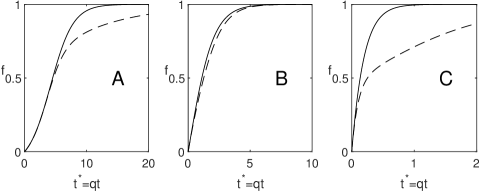
Figure 5. Aggregate adoption in the heterogeneous (dashes) compartmental network (96) is slower than in the corresponding homogeneous (solid) network (8). A) $p=0.1q$. B) $p=q$. C) $p=10q$.

Numerical simulations of (96) confirm that $f^{\rm het}(t)<f^{\rm hom}(t)$ for $p\geq q$ (Figure 5B-C). Moreover, they show that $f^{\rm het}(t)<f^{\rm hom}(t)$ for $p<q$ as well (Figure 5A). This suggests, therefore, that perhaps in the mildly-heterogeneous case (87), $f^{\rm het}<f^{\rm hom}$ for any $\{p_{k}\}$ and $\{q_{k}\}$, and not just when they are positively monotonically related. Whether this is the case, however, is currently open. A proof of Lemma 14 for $p<q$ is also open.

7. Discussion

The problem of proving that solutions of a system of master equations converge, as the number of individuals tends to infinity, to solutions of a compartmental model has been widely studied in many disciplines. The case most relevant for the Bass model for the diffusion of new products is that of the susceptible infected (SI) model in epidemiology [23], in which susceptible individuals correspond to nonadopters and infectives correspond to adopters. Some epidemiological models also include recovered individuals which correspond to “non-contagious” adopters, a category not included in the Bass model, but included in the Bass-SIR model [11, 12].

The approach developed here for proving that convergence consists of three steps.

1. The full set (6) of master equations for the probabilities of the states of all subsets of nodes is reduced to equations for a smaller set of variables, which is sufficient in the sense that the expected fraction of adopters can be written in terms of them, and is closed in the sense that the equations for those variables involve only those variables. The reduced equations for the homogeneous complete network are (14); for the homogeneous circle network are (40), and for the heterogeneous complete network are (65).

2. The reduced equations, which are a finite system of ODEs, are embedded into an infinite system of ODEs and the convergence of that system to the infinite limit system is proven.

3. An ansatz, such as (18) for the homogeneous complete network, (42) for the homogeneous circle network, and (68) for the heterogeneous complete network, provides an exact closure of the infinite limit system, which reduces that system to the compartmental model.

Regarding the analogous problem of proving convergence of epidemiological models to their mean field limits, there are several works with a variety of methods. To the best of our knowledge, all of these studies only considered homogeneous complete networks, and it is not clear whether their methods can be extended to other types of networks. In contrast, our methodology can be applied to various types of networks, with only minor modifications.

The most similar work to ours is [23], in which Simon and Kiss used an ODE approach to prove the convergence of the SIS model on complete networks to its compartmental limit. The key difference between their approach and ours is that our starting point are the master equations for the probabilities of the states of all subsets of nodes (a bottom-up approach), whereas Simon and Kiss started from the master equations for the probability of having $k$ adopters in the system at time $t$ (a top-down approach). It is not clear, however, whether a top-down approach can be extended to other types of netowrks beyond homogeneous complete networks, without introdcing a closure which is not rogorously justified. Other approaches for proving convergence of epidemiological models on homogeneous complete networks include a PDE approach [9, 23, 24], a stochastic approach [10, 17, 18, 23], and an elementary ODE approach that only requires a finite number of ODEs [2].

We now discuss the general problem of deducing convergence of solutions of finite systems of ODEs to those of infinite systems of ODEs. The formal limit system as $M\to\infty$ of a system of $M$ ODEs and initial conditions is the infinite system obtained by taking the limit of the equation and initial condition for each $u_{k}$ separately, with all components $u_{j}$ considered to be fixed.

Not surprisingly, if the component differential equations or initial conditions do not converge formally, then the solutions of the finite system may not converge. For example, if $\tfrac{d\hfill}{dt}u_{k}=M-u_{k}$ for $1\leq k\leq M$ and $u_{k}(0)=0$, then for $t>0$ the solutions $u_{k}(t)=M(1-e^{-t})$ of the finite system tend to infinity as $M\to\infty$. Similarly, if the initial value of $u_{M}$ is chosen sufficiently large then solutions of the finite system may tend to infinity even though the system converges formally to a limit system. For example, let

$$\tfrac{d\hfill}{dt}u_{k}=u_{k+1}\quad\text{and}\quad u_{k}(0)=0$$ (98)

for $1\leq k\leq M-1$, and let $\tfrac{d\hfill}{dt}u_{M}=0$ with $u_{M}(0)=(M!)^{2}$. For $M>k$ the ODE and initial condition for $u_{k}$ are (98) so the system tends formally to the infinite system in which (98) holds for all $k$. However, $u_{M-1}(t)=(M!)^{2}t$, $u_{M-2}(t)=(M!)^{2}\frac{t^{2}}{2}$, and by induction $u_{M-j}(t)=(M!)^{2}\frac{t^{j}}{j!}$, so setting $k=M-j$ yields $u_{k}(t)=\frac{(M!)^{2}t^{M}}{(M-k)!}$, which for $t>0$ tends to infinity with $M$.

Less obviously, the formal convergence of the component equations and initial conditions does not suffice in general to yield convergence of the solutions of the finite system to a specified soluton of the infinite system obtained as the formal limit, even when the initial data of the finite systems are bounded uniformly in $M$. This shows that the result of Theorem 7 is nontrivial. To demonstrate this phenomenon, consider the model system

$$\tfrac{d\hfill}{dt}u_{k}=a(k)(u_{k+1}-u_{k}),\qquad u_{k}(0)=1$$ (99)

for $1\leq k\leq M$, where the parameters $a(k)$ and the value used to replace the non-existent component $u_{M+1}$ appearing in the ODE for $u_{M}$ remain to be specified. For later use, note that solving (99) with $u_{k+1}$ considered to be a known function yields

$$u_{k}(t)=e^{-a(k)t}+a(k)e^{-a(k)t}\int_{0}^{t}u_{k+1}(s)e^{a(k)s}\,ds.$$ (100)

For any fixed $k$ the rule (99) applies for all $M\geq k+1$, so the formal limit system consists of (99) for all $1\leq k<\infty$, no matter what value is chosen for $u_{M+1}$. For any choice of the parameters $a(k)$ this limit system has a solution

$$u_{k}(t)\equiv 1\quad\text{for all $k$.}$$ (101)

However, we will show that for certain parameters $a(k)$ and values used to replace $u_{M+1}$ the solutions of the finite systems do not converge to the specified solution (101) of the limit system. Our method does not show whether the solutions converge to a different solution of the limit system or do not converge.

Two plausible replacements for $u_{M+1}$ are the value

$$u_{M+1}\equiv 1$$ (102)

equal to the initial value of all components, and the value

$$u_{M+1}\equiv 0$$ (103)

which corresponds to simply deleting the non-existent variable $u_{M+1}$ from the ODE for $u_{M}$. When (102) is used then (101) holds for every fixed $k$ even when $M$ is finite, no matter how the parameters $a(k)$ are chosen, because the right sides of the ODEs in (99) are then identically zero.

When $a(k)=1$ for all $k$ and $u_{M}$ is determined by (103) then the solutions $u_{k}$ of the finite system are not exactly equal to (101), but they converge to that value as $M\to\infty$. To see this, solve the ODE for $u_{M}$ to obtain $u_{M}(t)=e^{-t}$, then substitute this result into (100) with $k=M-1$ to obtain $u_{M-1}=(1+t)e^{-t}$. By induction we obtain from (100) that $u_{M-j}(t)=P_{j}(t)e^{-t}$, where $P_{j}(t)$ is the Taylor polynomial approximation of $e^{t}$ whose highest term is $\frac{t^{j}}{j!}$. Setting $j=M-k$ yields $u_{k}(t)=P_{M-k}(t)e^{-t}$ for $1\leq k\leq M$. Since $P_{M-k}(t)$ converges to $e^{t}$ as $M\to\infty$, $u_{k}(t)$ tends to (101) in that limit.

When $a(k)=3^{k}$ and $u_{M+1}$ is given by (103) then the solutions $u_{k}$ can no longer be calculated explicitly, but we can obtain upper bounds that imply that the solutions do not converge to (101). The solution formula (100) yields $u_{M}=e^{-3^{M}t}$, and substituting this into (100) for $k=M-1$ yields $u_{M-1}(t)=e^{-3^{M-1}t}+\frac{3^{M-1}}{3^{M}-3^{M-1}}(e^{-3^{M-1}t}-e^{-3^{M}t})\leq 2e^{-3^{M-1}t}$. Assuming by induction that $u_{k+1}\leq 2e^{-3^{k+1}t}$ and substituting that estimate into (100) yields $u_{k}(t)\leq e^{-3^{k}t}+\frac{2\;3^{k}}{3^{k+1}-3^{k}}(e^{-3^{k}t}-e^{-3^{k+1}t})\leq 2e^{-3^{k}t}$, which confirms that the estimate $u_{k}(t)\leq 2e^{-3^{k}t}$ holds for all $k\leq M$. Since $2e^{-3^{k}t}<1$ for $t>\frac{\ln 2}{3^{k}}$, $u_{k}(t)$ does not converge to $1$ as $M\to\infty$.

8. Proof of Lemma 10

Proof.

Let $g:=f_{1}-f_{2}$. Define

$$E(s)\mathrel{:=}\begin{cases}s^{2}&s>0\\ 0&s\leq 0.\end{cases}$$ (104)

Then $E(g(t))$ is differentiable and

$$\tfrac{d\hfil}{dt}E(g(t)) \leq\begin{cases}2g(t)[H_{2}(f_{1})-H_{2}(f_{2})]&g(t)>0\\ 0&g(t)\leq 0\end{cases}$$ (105)

$$\leq\begin{cases}2g(t)L|g(t)|&g(t)>0\\ 0&g(t)\leq 0\end{cases}\quad=2LE(g(t)).$$

Hence $\frac{d\hfil}{dt}e^{-2Lt}E(g(t))\leq 0$, which can be integrated to yield $e^{-2Lt}E(g(t))\leq E(g(0))=0$ for $t>0$, which by the definition of $E$ implies that

$$g(t)\leq 0 t>0$$ for . (106)

Now suppose that there exists a positive $t_{*}$ at which $g(t_{*})\geq 0$. By (106), $g(t_{*})=0$. Hence, $t_{*}$ is a local maximum of $g$, and so $g^{\prime}(t_{*})=0$. However, for $t>0$, $g^{\prime}(t)<H_{2}(f_{2}+g)-H_{2}(f_{2})$, so $g^{\prime}<0$ whenever $g=0$ at a positive time. This contradiction shows that no such $t_{*}$ exists, and hence $f_{1}(t)-f_{2}(t)=g(t)<0$ for all $t>0$. ∎

Email address: fibich@tau.ac.il
Email address: amitgolan33@gmail.com
Email address: schochet@tauex.tau.ac.il

References

- [1] R. Albert, H. Jeong and A. Barabási, Error and attack tolerance of complex networks, Nature 406 (2000) 378–382.
- [2] B. Armbruster and E. Beck, An elementary proof of convergence to the mean-field equations for an epidemic model, IMA Journal of Applied Mathematics. 82 (2017) 152–157.
- [3] B. Armbruster and E. Beck, Elementary proof of convergence to the mean-field model for the SIR process, J. Math. Biol. 75 (2017) 327–339.
- [4] R. Anderson and R. May, Infectious Diseases of Humans (Oxford University Press, Oxford, 1992).
- [5] F. Bass, A new product growth model for consumer durables, Management Sci. 15 (1969) 1215–1227.
- [6] C. Bulte and Y. V. Joshi, New product diffusion with influentials and imitators, Marketing Science 26 (2007) 400–421.
- [7] R. Chatterjee and J. Eliashberg, The innovation diffusion process in a heterogeneous population: A micromodeling approach, Management Science 36 (1990) 1057–1079.
- [8] G. De Tarde, The laws of imitation (H. Holt, 1903).
- [9] O. Diekmann and J.A.P. Heesterbeek, Mathematical epidemiology of infectious diseases: model building, analysis and interpretation (John Wiley and Sons, Chichester, 2000).
- [10] S.N. Ethier and T.G. Kurtz, Markov Processes: Characterization and Convergence (John Wiley and Sons, USA, 2005)
- [11] G. Fibich, Bass-SIR model for diffusion of new products in social networks, Phys. Rev. E 94 (2016) 032305.
- [12] G. Fibich, Diffusion of new products with recovering consumers, SIAM J. Appl. Math. 77 (2017) 1230-1247.
- [13] G. Fibich and R. Gibori, Aggregate diffusion dynamics in agent-based models with a spatial structure, Oper. Res. 58 (2010) 1450–1468.
- [14] G. Fibich and A. Golan, Diffusion of new products with heterogeneous consumers, Mathematics of Operations Research. doi:10.1287/moor.2022.1261.
- [15] G. Fibich, T. Levin and O. Yakir, Boundary Effects in the Discrete Bass Model, SIAM J. Appl. Math. 79 (2019) 914–937.
- [16] M. Jackson, Social and Economic Networks (Princeton University Press, Princeton and Oxford, 2008).
- [17] T.G. Kurtz, Solutions of Ordinary Differential Equations as Limits of Pure Jump Markov Processes, Journal of Applied Probability. 7 (1970) 49–58.
- [18] T.G. Kurtz, Limit Theorems for Sequences of Jump Markov Processes Approximating Ordinary Differential Processes, Journal of Applied Probability. 8 (1971) 344–356.
- [19] V. Mahajan, E. Muller and F. Bass, New-product diffusion models, in Handbooks in Operations Research and Management Science, eds. J. Eliashberg and G. Lilien (North-Holland, Amsterdam, 1993), volume 5, pp. 349–408.
- [20] S. Niu, A stochastic formulation of the Bass model of new product diffusion, Math. Problems Engrg. 8 (2002) 249–263.
- [21] R. Pastor-Satorras and A. Vespignani, Epidemic spreading in scale-free networks, Phys. Rev. Lett. 86 (2001) 3200–3203.
- [22] E. Rogers, Diffusion of Innovations (Free Press, New York, 2003), fifth edition.
- [23] P. Simon and I. Kiss, From exact stochastic to mean-field ODE models: a new approach to prove convergence results, IMA J. Appl. Math., 78 (2013) 945–964.
- [24] P. Simon, M. Taylor, and I Kiss, Exact epidemic models on graphs using graph-automorphism driven lumping, J. Math. Biol., 62 (2011) 479–508.
- [25] D. Strang and S. Soule, Diffusion in organizations and social movements: From hybrid corn to poison pills, Annu. Rev. Sociol. 24 (1998) 265–290.
- [26] e. W.J. Hopp, Ten most influential papers of management science’s first fifty years, Management Sci. 50 (2004) 1763–1893.