A Moving Window Based Approach to Multi-scan Multi-Target Tracking

Abstract

Multi-target state estimation refers to estimating the number of targets and their trajectories in a surveillance area using measurements contaminated with noise and clutter. In the Bayesian paradigm, the most common approach to multi-target estimation is by recursively propagating the multi-target filtering density, updating it with current measurements set at each timestep. In comparison, multi-target smoothing uses all measurements up to current timestep and recursively propagates the entire history of multi-target state using the multi-target posterior density. The recent Generalized Labeled Multi-Bernoulli (GLMB) smoother is an analytic recursion that propagate the labeled multi-object posterior by recursively updating labels to measurement association maps from the beginning to current timestep. In this paper, we propose a moving window based solution for multi-target tracking using the GLMB smoother, so that only those association maps in a window (consisting of latest maps) get updated, resulting in an efficient approximate solution suitable for practical implementations.

I Introduction

In the Bayesian approach to single-target tracking, the current state (represented by a vector) of the target conditioned on the history of measurements is recursively propagated in time via the filtering density [1, 4]. On the other hand, in the multi-scan approach (to single-target tracking) the entire history of the single-target state (conditioned on the history of measurements) is recursively propagated via the smoothing density [28]. Analogously, in the multi-target state estimation, multi-target state is propagated using the multi-object filtering density [29] and multi-object smoothing density [33], where the multi-target state and observations are represented as Random Finite Sets (RFSs) [18][19].

The Generalized Labeled Multi-Bernoulli (GLMB) filter [29, 30] is an analytic solution to the multi-object filtering density that can be used to estimate multi-target state with target labels (identities). An efficient implementation of the GLMB filter has been proposed in [31] by sampling its components using a Gibbs sampler [7]. This approach was demonstrated to track over a millions targets from about a billion detections in relatively challenging signal scenarios [2]. Due to its versatility and efficiency, the GLMB filter has been extended to track before detect [26, 16], distributed tracking [9, 15], tracking with lineage [24, 5], as well as applied to computer vision [14, 12, 25], Doppler tracking [8, 37], field robotics [20, 21], space situational awareness [34, 35, 10, 11], multi-object sensor scheduling and path planning [3, 22, 6, 23, 36].

A recent research avenue is GLMB smoothing [33], where Gibbs sampling was used to solve multi-dimensional assignment problem in multi-scan multi-object tracking. In addition, this Gibbs sampler was combined with importance to solve the multi-dimensional assignment problem in multi-sensor multi-object tracking [32]. The labeled multi-object states caters for trajectories, and smoothing improves the multi-object states in the all past timesteps as the smoothing density is updated with future information. However, even with single-target smoothing, the computation cost at each timestep increases, and may result in an unaffordable computational cost for practical implementation. In the multi-target state estimation, smoothing poses and even more difficult NP-hard multi-dimensional assignment problem that keeps increasing its complexity with every timestep. Therefore, it is desirable to come up with a multi-target smoothing approach with an approximately similar computational cost per each update step.

In this paper, we propose a novel technique to propagate the multi-object smoothing density with similar computational cost at each timestep. Instead of updating the entire history of the multi-object state trajectory, we only update the latest $N$ scans of the multi-object history. Since the target trajectories in the GLMB smoother are characterised by association maps (see Section II), we propose to link the trajectories in the posterior using a moving window based method.

Section II summarizes the background information related to multi-object state estimation, Section III explains the implementation details of the proposed moving window based multi-target tracker and presents the pseudo code for the moving window based smoother. Section IV presents the numerical results, and Section V concludes the paper.

II Background

We follow the same convention as in [33], and summarize the symbols, notations and definitions in this section. For a given set $S$, $\mathcal{F}(S)$ denotes the class of finite subsets of $S$, $1_{S}(\cdot)$ denotes the indicator function, $\delta_{X}[Y]$ denotes Kroneker-$\delta$ function, where $\delta_{X}[Y]=1$ if $X=Y$, 0 otherwise, and $\langle f,g\rangle$ denotes the inner product, i.e., $\int f(x)g(x)dx$, of two functions $f$ and $g$. The list of variables $X_{m},X_{m+1},...,X_{n}$ is abbreviated as $X_{m:n}$, the cardinality of a finite set $X$ is denoted as $|X|$, and for some function $f$, the product $\prod_{x\in X}f(x)$ is denoted by the (single scan) multi-object exponential $f^{X}$, with $f^{\emptyset}=1$.

II-A Mulit-object States and Trajectories

Let $\mathbb{X}$ denote the single object state space, $\mathbb{L}_{k}$ denote the space of all labels at time $k$, and $\mathbb{B}_{k}$ denote the space of all birth labels at time $k$. Then, the label space for all objects up to time $k$ is given by $\mathbb{L}_{k}=\biguplus\nolimits_{s=0}^{k}\mathbb{B}_{s}$ (note that $\mathbb{L}_{k}=\mathbb{L}_{k-1}\uplus\mathbb{B}_{k}$), and a labeled state of an object existing at time $k$ is given by $\boldsymbol{x}=(x,\ell)\in\mathbb{X}\mathcal{\times}\mathbb{L}_{k}$, where the vector $x\in\mathbb{X}$ is its kinematic state and $\ell=(s,\iota)$ is a unique label, $s$ is the time of birth, and $\iota$ is a unique index to distinguish objects born at the same time. A sequence of labeled states at consecutive times ($s$ to $t$)

$$\mathbf{\tau}=[(x_{s},\ell),(x_{s+1},\ell),...,(x_{t},\ell)],$$ (1)

with the common label $\ell$ and states $x_{s},x_{s+1},...,x_{t}\in\mathbb{X}$ is called a trajectory.

A labeled multi-object state at time $i$ is a finite subset $\boldsymbol{X}_{i}$ of $\mathbb{X}\mathcal{\times}\mathbb{L}_{i}$ with distinct labels. Let $\mathcal{L\,}$:$\mathcal{\,}\mathbb{X}\mathcal{\times}\mathbb{L}_{i}\!\rightarrow\!\mathbb{L}_{i}$ is the projection defined by $\mathcal{L}((x,\ell))\!=\ell$, and $\mathcal{L}(\boldsymbol{X}_{i})$ is the set of lables of $\boldsymbol{X}_{i}$. Note that, a valid $\boldsymbol{X}_{i}$ has distinct labels and results in the distinct label indicator $\Delta(\boldsymbol{X}_{i})\!\triangleq\delta_{|\boldsymbol{X}_{i}|}[|\mathcal{L(}\boldsymbol{X}_{i})|]$ to be equals to one. The labeled multi-object state can also be written as $\boldsymbol{X}_{i}=\left\{\mathbf{\tau(}i\mathbf{)\mathcal{\,}}\text{:}\mathbf{\mathcal{\,}\tau\in}S\right\}$, where $S$ is a set of trajectories defined to have kinematic states and distinct labels at each timestep, and $\mathbf{\tau(}i\mathbf{)}$ denotes the labeled state of trajectory $\mathbf{\tau}$ at time $i$. The trajectory of the object with label $\ell\in\cup_{i=j}^{k}\mathcal{L}(\boldsymbol{X}_{i}\mathbf{)}$ in a given sequence $\boldsymbol{X}_{j:k}$ of labeled multi-object states in the interval $\{j\mathcal{\,}$:$\mathcal{\,}k\}$ is given by:

$$\boldsymbol{x}_{s(\mathbf{\ell}):t(\mathbf{\ell})}^{(\mathbf{\ell})}=[(x_{s(\mathbf{\ell})}^{(\mathbf{\ell})},\mathbf{\ell}),...,(x_{t(\mathbf{\ell})}^{(\mathbf{\ell})},\mathbf{\ell})],$$ (2)

where $s(\mathbf{\ell})$ and $t(\mathbf{\ell})$ are respectively the earliest and latest times the label $\mathbf{\ell}$ exists on the interval $\{j\mathcal{\,}$:$\mathcal{\,}k\}$, and $\boldsymbol{x}_{i}^{(\mathbf{\ell})}=(x_{i}^{(\mathbf{\ell})},\mathbf{\ell})$ denotes the element of $\boldsymbol{X}_{i}$ with label $\ell\in\mathcal{L}(\boldsymbol{X}_{i}\mathbf{)}$ with unlabeled state $x_{i}^{(\mathbf{\ell})}$. The sequnce $\boldsymbol{X}_{j:k}$ can thus be equivalently represented by the set of all trajectories

$$\boldsymbol{X}_{j:k}\equiv\left\{\boldsymbol{x}_{s(\mathbf{\ell}):t(\mathbf{\ell})}^{(\mathbf{\ell})}:\ell\in\bigcup\nolimits_{i=j}^{k}\mathcal{L}(\boldsymbol{X}_{i}\mathbf{)}\right\},$$ (3)

of all labels in $\cup_{i=j}^{k}\mathcal{L}(\boldsymbol{X}_{i})$. Furthermore, for any function $h:\uplus_{I\subseteq\{j:k\}}\mathbb{T}_{I}\rightarrow[0,\infty)$, the multi-scan multi-object exponential [33] is defined as

$$[h]^{\boldsymbol{X}_{j:k}}\triangleq[h]^{\{\boldsymbol{x}_{s(\ell):t(\ell)}^{(\ell)}:\ell\in\mathcal{L}(\boldsymbol{X}_{j:k})\}}=\underset{\ell\in\mathcal{L}(\boldsymbol{X}_{j:k})}{\prod}h(\boldsymbol{x}_{s(\ell):t(\ell)}^{(\ell)}),$$

where for any non-negative integer $n$ and $i_{1}<i_{2}<...<i_{n}$, $\mathbb{T}_{\{i_{1},i_{2},...,i_{n}\}}\triangleq\big{(}\mathbb{X}\times\mathbb{L}_{i_{1}}\big{)}\times....\times\big{(}\mathbb{X}\times\mathbb{L}_{i_{n}}\big{)}$, with $\mathbb{T}_{\emptyset}=\emptyset$. If $j=k$, the multi-scan exponential reduces to single-scan multi-object exponential $h^{\boldsymbol{X}_{j}}$ defined above.

II-B Multi-object System Model

Given the multi-object state $\boldsymbol{X}_{k-1}$ at time $k-1$, each object with state $\boldsymbol{x}_{k-1}=(x_{k-1},\ell_{k-1})\in\boldsymbol{X}_{k-1}$ either survies with probability $P_{S,k-1}(\boldsymbol{x}_{k-1})$ and moves to a new state $\boldsymbol{x}_{k}=(x_{k},\ell_{k})$ with transition density $f_{S,k|k-1}(x_{k}|x_{k-1},\ell_{k})\delta_{\ell_{k-1}}[\ell_{k}]$, or dies with probability $Q_{S,k-1}(\boldsymbol{x}_{k-1})=1-P_{S,k-1}(\boldsymbol{x}_{k-1})$ at time $k$. Further, each object with label $\ell_{k}$ in birth label space $\mathbb{B}_{k}$ is either born with probability $P_{B,k}(\ell_{k})$ and state $x_{k}$ with probability density $f_{B,k}(x_{k},\ell_{k})$, or not born with probability $Q_{B,k}(\ell_{k})=1-P_{B,k}(\ell_{k})$ at time $k$. Thus, the multi-object state $\boldsymbol{X}_{k}$ at time $k$ is the superposition of the suviving states and new birth states, and in the standard multi-object dynamic model, the birth and survival sets are independent of each other, and each object moves and dies independently of each other. The multi-object transition density $\boldsymbol{f}_{k|k-1}(\boldsymbol{X}_{k}|\boldsymbol{X}_{k-1})$ captures the multi-object dynamic model, and see [33, 29] its detailed expressions.

II-C Multi-object Observation Model

Let $\boldsymbol{X}_{k}$ and $Z_{k}$ be the multi-object state at time $k$, and the set of measurements captured by the sensor. Each object $\boldsymbol{x}\in\boldsymbol{X}_{k}$ either generates a measurement $z\in Z_{k}$ (with detection probability $P_{D}(\boldsymbol{x})$) on the measurement space $\mathbb{Z}$ with likelihood $g_{k}(z|\boldsymbol{x})$ or miss-detected (with probability $Q_{D}(\boldsymbol{x})=1-P_{D}(\boldsymbol{x})$). Additionally, the sensor also produces measurement clutter, which is modeled by a Poisson RFS with intensity function $\kappa_{k}$ on $\mathbb{Z}$. Conditional on $\boldsymbol{X}_{k}$, the detections and measurement clutter are independent, and therefore multi-object observation $Z_{k}$ is the superposition of them.

A map of the form $\gamma_{k}:\mathbb{L}_{k}\rightarrow\{-1:|Z_{k}|\}$ is called an association map if it is positive 1-1 (i.e., no two distinct labels are mapped to the same positive value). If $\ell$ generates the $\gamma_{k}(\ell)$-th measurement $\gamma_{k}(\ell)>0$, if $\ell$ is misdetected $\gamma_{k}(\ell)=0$, and if $\ell$ does not exist $\gamma_{k}(\ell)=-1$. Then, the multi-object likelihood function is

$$g_{k}(Z_{k}| \boldsymbol{X}_{k})\propto\underset{\gamma_{k}\in\Gamma_{k}}{\sum}\delta_{\mathcal{L}(\gamma_{k})}[\mathcal{L}(\boldsymbol{X}_{k})][\psi_{k,Z_{k}}^{(\gamma_{k}\circ\mathcal{L}(\cdot))}(\cdot)]^{\boldsymbol{X}_{k}},$$ (4)

where $\mathcal{L}(\gamma_{k})\triangleq\{\ell\in\mathbb{L}_{k}:\gamma_{k}(\ell)\geq 0\}$ is the set of live labels of $\gamma_{k}$, and $\Gamma_{k}$ is the space of all association maps, $\gamma_{k}\circ\mathcal{L}(\cdot)=\gamma_{k}(\mathcal{L}(\cdot))$ and

$$\psi_{k,\{z_{1:m}\}}^{(i)}(\boldsymbol{x})=\begin{cases}\frac{P_{D}(\boldsymbol{x})g_{k}(z_{i}|\boldsymbol{x})}{\kappa_{k}(z_{i})}&i>0\\ Q_{D,k}(\boldsymbol{x})&i=0\end{cases}.$$ (5)

II-D Trajectory Posterior of a Single Object

The GLMB posterior is written in terms of single object periors, and the corresponding association weights [33]. Thus, it is informative to take a close look at the trajectory posterior and the association weight of an object with label $\ell\in\mathbb{L}_{k}$, before the presenting the GLMB posterior. Recall that $s(\ell)$ and $t(\ell)$ respectively denote the earliest and latest times on $\{0:k\}$ such that $\ell$ exists. Assuming that $\ell$ generates the sequence of measurement indices $\alpha_{s(\ell):k}$, its trajectory posterior at time $k$ can be in one of four possible stages: (i) new born, $s(\ell)=k$; (ii) surviving, $t(\ell)=k>s(\ell)$; (iii) die at time $k$, $t(\ell)=k-1$; (iv) died before time $k$, $t(\ell)<k-1$. Thus, its trajectory posterior at time $k$ is given by,

$$\tau{}_{0:k}^{(\alpha_{s(\ell):k})}(x_{s(\ell):t(\ell)},\ell)$$ (6)

$$=\begin{cases}\negthinspace\frac{\Lambda_{B,k}^{(\alpha_{k})}(x_{k},\ell)}{\bar{\Lambda}_{B,k}^{(\alpha_{k})}(\ell)},&\negthinspace\negthinspace\negthinspace\negthinspace\negthinspace s(\ell)=k\\ \negthinspace\frac{\Lambda_{S,k|k-1}^{(\alpha_{k})}(x_{k}|x_{k-1},\ell)\tau_{0:k-1}^{(\alpha_{s(\ell):k-1})}(x_{s(\ell):k-1},\ell)}{\bar{\Lambda}_{S,k|k-1}^{(\alpha_{s(\ell):k})}(\ell)},&\negthinspace\negthinspace\negthinspace\negthinspace\negthinspace t(\ell)=k>s(\ell)\\ \negthinspace\frac{Q_{S,k-1}(x_{k-1},\ell)\tau_{0:k-1}^{(\alpha_{s(\ell):k-1})}(x_{s(\ell):k-1},\ell)}{\bar{Q}_{S,k-1}^{(\alpha_{s(\ell):k-1})}(\ell)},&\negthinspace\negthinspace\negthinspace\negthinspace\negthinspace t(\ell)=k-1\\ \negthinspace\tau_{0:t(\ell)}^{(\alpha_{s(\ell):t(\ell)})}(x_{s(\ell):t(\ell)},\ell),&\negthinspace\negthinspace\negthinspace\negthinspace\negthinspace t(\ell)<k-1\end{cases},$$

where $\tau_{0:k}^{(\alpha_{s(\ell):k-1})}(x_{s(\ell):k-1},\ell)$ is the trajectory posterior at time $k-1$,

$$\Lambda_{B,k}^{(\alpha_{k})}(x,\ell)= \ \psi_{k,Z_{k}}^{(\alpha_{k})}(x,\ell)P_{B,k}(\ell)f_{B,k}(x,\ell),$$ (7)

$$\bar{\Lambda}_{B,k}^{(\alpha_{k})}(\ell)= \int\Lambda_{B,k}^{(\alpha_{k})}(x,\ell)dx,$$ (8)

$$\Lambda{}_{S,k|k-1}^{(\alpha_{k})}(x_{k}|x_{k-1},\ell)= \ \psi_{k,Z_{k}}^{(\alpha_{k})}(x_{k},\ell)P_{S,k-1}(x_{k-1},\ell)$$ (9)

$$\times \ f_{S,k|k-1}(x_{k}|x_{k-1},\ell),$$

$$\bar{\Lambda}{}_{S,k|k-1}^{(\alpha_{s(\ell):k})}(\ell)= \int\tau_{0:k-1}^{(\alpha_{s(\ell):k-1})}(x_{s(\ell):k-1},\ell)$$ (10)

$$\times \ \Lambda_{S,k|k-1}^{(\alpha_{k})}(x_{k}|x_{k-1},\ell)dx_{s(\ell):k},$$

$$\bar{Q}{}_{S,k-1}^{(\alpha_{s(\ell):k-1})}(\ell)= \int\tau_{0:k-1}^{(\alpha_{s(\ell):k-1})}(x_{s(\ell):k-1},\ell)$$ (11)

$$\times \ Q_{S,k-1}(x_{k-1},\ell)dx_{s(\ell):k-1}.$$

The association weight of $\ell$ is given by

$$\eta_{k|k-1}^{(\alpha_{s(\ell):k})}(\ell)=\begin{cases}\bar{\Lambda}_{B,k}^{(\alpha_{k})}(\ell),&\negthinspace\negthinspace\negthinspace\negthinspace s(\ell)=k\\ \bar{\Lambda}_{S,k|k-1}^{(\alpha_{s(\ell):k})}(\ell),&\negthinspace\negthinspace\negthinspace\negthinspace t(\ell)=k>s(\ell)\\ \bar{Q}_{S,k-1}^{(\alpha_{s(\ell):k-1})}(\ell),&\negthinspace\negthinspace\negthinspace\negthinspace t(\ell)=k-1\\ Q_{B,k}(\ell),&\negthinspace\negthinspace\negthinspace\negthinspace\ell\in\mathbb{B}_{k},\alpha_{k}=-1{}^{V}\end{cases}\negthinspace\negthinspace.$$ (12)

II-E Multi-object Bayes Recursion

Given the observation history $Z_{1:k}$, the multi-object posterior $\boldsymbol{\pi}_{0:k}(\boldsymbol{X}_{\negthinspace 0:k})\triangleq\boldsymbol{\pi}_{0:k}(\boldsymbol{X}_{\negthinspace 0:k}|Z_{1:k})$ captures all information about the set of objects in the surveillance region in the interval {$0:k\}$. It can be written in the recursive form

$$\boldsymbol{\pi}_{0:k}(\boldsymbol{X}_{\negthinspace 0:k})\propto g_{k}(Z_{k}|\boldsymbol{X}_{\negthinspace k})\boldsymbol{f}_{k|k-1}(\boldsymbol{X}_{\negthinspace k}|\boldsymbol{X}_{\negthinspace k-1})\boldsymbol{\pi}_{0:k-1}(\boldsymbol{X}_{\negthinspace 0:k-1}).$$ (13)

The GLMB smoother [33] was proposed to as an analytic solution to the multi-object posterior recursion. Assuming that there are no live objects at the beginning, i.e., $\boldsymbol{\pi}_{0}(\boldsymbol{X}_{0})=\delta_{0}[\mathcal{L}(\boldsymbol{X}_{0})]$ with weight $w_{0}^{(\gamma_{0})}=1$, the GLMB posterior at time $k$ is given by [33]

$$\boldsymbol{\pi}_{0:k}(\boldsymbol{\boldsymbol{X}}_{0:}{}_{k})\propto$$ (14)

$$\ \ \ \ \Delta(\boldsymbol{X}_{0:k})\underset{\gamma_{0:k}}{\sum}w_{0:k}^{(\gamma_{0:k})}\delta_{\mathcal{L}(\gamma_{0:k})}[\mathcal{L}(\boldsymbol{X}_{0:k})][\tau_{0:k}^{(\gamma_{0:k}\circ\mathcal{L}(\cdot))}(\cdot)]^{\boldsymbol{X}_{0:k}},$$

where $\Delta(\boldsymbol{X}_{0:k})\triangleq\prod_{i=0}^{k}\Delta(\boldsymbol{X}_{i})$, and

$$\negthinspace\negthinspace\negthinspace\negthinspace w_{0:k}^{(\gamma_{0:k})}= \prod_{j=1}^{k}w_{j}^{(\gamma_{0:j})},$$ (15)

$$\negthinspace\negthinspace\negthinspace\negthinspace w_{j}^{(\gamma_{0:j})}= 1_{\mathcal{F}(\mathbb{B}_{j}\uplus\mathcal{L}(\gamma_{j-1}))}(\mathcal{L}(\gamma_{j}))[\eta_{j|j-1}^{(\gamma_{0:j}(\cdot))}(\cdot)]^{\mathbb{B}_{j}\uplus\mathcal{L}(\gamma_{j-1})}.$$ (16)

It is clear that the GLMB posterior is completely parameterized by the set of components $\{(w_{0:k}^{(\gamma_{0:k})},\tau_{0:k}^{(\gamma_{0:k})})\}$ indexed by $\gamma_{0:k}$. As per (13) the number of such components grow exponentially after each measurement update step, and to achieve tractability, truncation is performed and retain the highest weighted components [33].

III Computing the GLMB Posterior

In this section, we summarize the Gibbs sampler proposed in [33] to truncate the GLMB posterior.

III-A Sampling Distributions

The GLMB posterior is truncated from some discrete probability distribution $\pi$ of association maps $\gamma_{0:k}$, so that those maps with higher weights are more likely to be chosen. Starting with $\mathcal{L}(\gamma_{0})=\emptyset$, we consider

$$\pi(\gamma_{0:k})= \ \overset{k}{\underset{j=1}{\prod}}\pi^{(j)}(\gamma_{j}|\gamma_{0:j-1})\propto w_{0:k}^{(\gamma_{0:k})},$$ (17)

where

$$\pi^{(j)}(\gamma_{j}|\gamma_{0:j-1})\propto \ w_{j}^{(\gamma_{0:j})}$$ (18)

$$\propto \ 1_{\Gamma_{j}}(\gamma_{j})1_{\mathcal{F}(\mathbb{B}_{j}\uplus\mathcal{L}(\gamma_{j-1}))}(\mathcal{L}(\gamma_{j}))$$

$$\times \ [\eta_{j|j-1}^{(\gamma_{0:j}(\cdot))}(\cdot)]^{\mathbb{B}_{j}\uplus\mathcal{L}(\gamma_{j-1})}.$$

The term $1_{\Gamma_{j}}(\gamma_{j})$ makes sure that $\gamma_{j}$ is in the space of all association maps at time $j$, and $1_{\mathcal{F}(\mathbb{B}_{j}\uplus\mathcal{L}(\gamma_{j-1}))}(\mathcal{L}(\gamma_{j}))$ makes sure that only values of $\gamma_{j}$ on $\mathbb{B}_{j}\uplus\mathcal{L}(\gamma_{j-1})$ need to considered.

Given a valid $\gamma_{0:k}$, the Gibbs sampler constructs a sequence of iterates, such that the next iterate $\gamma_{0:k}^{{}^{\prime}}$ is generated from $\gamma_{0:k}$ by sampling each $\gamma_{j}^{{}^{\prime}}(\ell_{n})$ from the conditional

$$\pi_{j,n}(\alpha| \overbrace{\gamma_{0:j-1}^{{}^{\prime}}}^{\mathrm{past}},\overbrace{\gamma_{j}^{{}^{\prime}}(\ell_{1:n-1})}^{\mathrm{current\ (processed)}},\overbrace{\gamma_{j}(\ell_{n+1:|\mathbb{L}_{j}|})}^{\mathrm{current\ (unprocessed)}},\overbrace{\gamma_{j+1:k}}^{\mathrm{future}})$$

$$\propto \ \pi(\gamma_{0:j-1}^{{}^{\prime}},\gamma_{j}^{{}^{\prime}}(\ell_{1:n-1}),\alpha,\gamma_{j}(\ell_{n+1:|\mathbb{L}_{j}|}),\gamma_{j+1:k})$$ (19)

for each $j\in\{1:k\}$, $\ell_{n}\in\{\ell_{1:|\mathbb{L}_{j}|}\}$. Let $\gamma_{\bar{j}}\triangleq(\gamma_{0:j-1},\gamma_{j+1:k})$,

$$\eta_{j,n}^{(\gamma_{\bar{j}})}(\alpha)\triangleq\negthinspace\negthinspace\overset{k\lor(t(\ell_{n})+1)}{\underset{i=j}{\prod}}\negthinspace\negthinspace\eta_{j|j-1}^{(\gamma_{0:j-1}(\ell_{n}),\alpha,\gamma_{j+1:i}(\ell_{n}))}(\ell_{n}),\negthinspace\negthinspace\negthinspace$$ (20)

$$M_{\beta}^{(S)}(\alpha)\triangleq\begin{cases}\delta_{\beta}[\alpha],&\alpha<0\\ 1,&\alpha=0\\ (1-1_{S}(\alpha)&\alpha>0\end{cases},$$

where $a\lor b$ denotes $\text{min}\{a,b\}$. Consider $\gamma_{j}$ of the valid association history $\gamma_{0:k}$, $j\in\{1:k\}$. Then, for any $\ell_{n}\in\mathbb{L}_{j}-(\mathbb{B}_{j}\uplus\mathcal{L}(\gamma_{j-1})),$ the conditional (19) is given by,

$$\pi_{j,n}(\gamma_{j}(\ell_{n} )|\gamma_{j}(\ell_{\bar{n}}),\gamma_{\bar{j}})$$ (21)

$$= \ \delta_{-1}[\gamma_{j}(\ell_{n})]\delta_{\gamma_{\mathrm{min}\{j+1,k\}}(\ell_{n})}[\gamma_{j}(\ell_{n})],$$

and for $\ell_{n}\in\mathbb{B}_{j}\uplus\mathcal{L}(\gamma_{j-1})$

$$\pi_{j,n}( \gamma_{j}(\ell_{n})|\gamma_{j}(\ell_{\bar{n}}),\gamma_{\bar{j}})$$ (22)

$$= \ \eta_{j,n}^{(\gamma_{\bar{j}})}(\gamma_{j}(\ell_{n}))M_{\gamma_{\mathrm{min}\{k,j+1\}}(\ell_{n})}^{(\gamma_{j}(\ell_{\bar{n}}))}(\gamma_{j}(\ell_{n})),$$

and set $\gamma_{j}(\ell_{n})=-1$ for all other $\ell_{n}$.

III-B Computing the Posterior

It is clear that as the time interval, i.e., $\{0:k\}$, grows, the dimensionality of the GLMB posterior (13) increases and it becomes impractical to compute the entire posterior at each timestep using (17). In this work, we propose to mitigate this computational complexity by smoothing over fixed windows, while linking the trajectory estimates between windows using their labels and corresponding association maps. This approach is illustrated in Fig. 1, which results in a computationally efficient approximate solution to the GLMB posterior propagation.

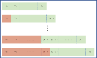
Figure 1: Moving window approach with window size $N$. Maps shaded in brown are not updated.

Given an intial $\gamma_{0:k}$, a set of new samples can be generated based on this technique by using Algorithm 1. There are two methods to further improve the computational efficiency of Algorithm 1. In the first method, since there exist duplicate trajectories, i.e., those with the same association history and label combination, the corresponding trajectory and weight information can be stored and reused instead of calcuating them each time. The second method is to paralallelize Algorithm 1, so that each new sample based on $\gamma_{0:k}$ is simultaneously generated instead of generating one after another.

Furthermore, Algorithm 1 can also be used with a smoothing-while-filtering approach as shown in Algorithm 2. Note that the function $\mathrm{SampleFactors}$ (in Algorithm 2) is given in [33].

inputs: $G_{0:k}=(\gamma_{0:k},w_{0:k},\tau_{0:k})$, $T$ (no. samples)

output: $[G_{0:k}^{(t)}]_{t=1}^{T}=[(\gamma_{0:k}^{(t)}),w_{0:k}^{(t)},\tau_{0:k}^{(t)}]_{t=1}^{T}$

for $t=1:T$

for $j=k-N+1:k$

$P_{j}\coloneqq|\mathbb{B}_{j}\uplus\mathcal{L}(\gamma_{j-1})|$; $M_{j}\coloneqq|Z_{j}|$;

$c:=-1:M_{j}$; $\gamma^{\prime}_{j}=[\ ]$;

for $n=1:P_{j}$

for $\alpha=-1:M_{j}$

$\varkappa(\alpha):=\pi_{j,n}(\alpha|\gamma_{j}^{{}^{\prime}}(\ell_{1:n-1}),\gamma_{j}(\ell_{n+1:P_{j}}),\gamma_{\bar{j}});$

via (22)

end

$\gamma^{\prime}_{j}(\ell_{n})\propto$ $\ \mathrm{Categorical}$$(c,\varkappa);$ $\gamma_{j}^{{}^{\prime}}:=[\gamma_{j}^{{}^{\prime}};\gamma_{j}^{{}^{\prime}}(\ell_{n})];$

end

$\gamma_{j}:=\gamma_{j}^{{}^{\prime}};$ $\gamma_{0:j}:=[\gamma_{0:j-1},\gamma_{j}];$

compute $w_{0:k}$, $\tau_{0:k}$ via (12) and (6)

end

$G_{0:k}^{(t)}:=(\gamma_{0:k},w_{0:k},\tau_{0:k});$

end

Algorithm 1 Windowed-MultiScanGibbs

input: $[G_{0:k-1}^{(h)}]_{h=1}^{H_{k-1}}$, $[T^{(h)}]_{h=1}^{H_{k-1}}$, $T$

output: $[G_{0:k}^{(h)}]_{h=1}^{H_{k}}$

for $h=1:H_{k-1}$

$[G_{0:k}^{(h,t)}]_{t=1}^{\tilde{T}^{(h)}}\coloneqq\mathrm{Unique}(\mathrm{SampleFactors}(G_{0:k}^{(h)},T^{(h)}));$

end

if $k<N,$

keep $H_{k}$ best $[G_{0:k}^{(h)}]_{h=1}^{H_{k}}$

normalize weights $[w_{0:k}^{(h)}]_{h=1}^{H_{k}}$

return

end

keep $\bar{H}_{k}$ best $[G_{0:k}^{(h)}]_{h=1}^{\bar{H}_{k}}$

for $h=1:\bar{H}_{k}$

$[G_{0:k}^{(h,t)}]_{t=1}^{T}\coloneqq\mathrm{WinMultiScanGibbs}(G_{0:k}^{(h)},T);$

end

$[G_{0:k}^{(t)}]_{t=1}^{\tilde{T}}\coloneqq\mathrm{Unique}([G_{0:k}^{(h,t)}]_{h,t=(1,1)}^{(\bar{H}_{k},T)});$

keep $H_{k}$ best $[G_{0:k}^{(h)}]_{h=1}^{H_{k}};$

normalize weights $[w_{0:k}^{(h)}]_{h=1}^{H_{k}}$

Algorithm 2 Windowed-Smoothing-while-Filtering

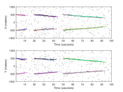
(a) Filtering

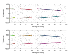
(b) Smoothing (window size = 5)

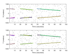
(c) Smoothing (window size = 20)

Figure 2: Estimated trajectories (superimposed on the ground truth - solid lines) from GLMB filtering and GLMB smoothing with window sizes 5 and 20.

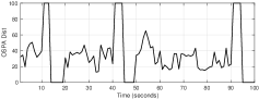
(a) Filtering

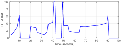
(b) Smoothing (window size = 5)

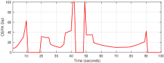
(c) Smoothing (window size = 20)

Figure 3: OSPA performance from GLMB filtering and GLMB smoothing with window sizes 5 and 20.

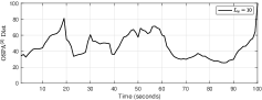
(a) Filtering

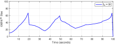
(b) Smoothing (window size = 5)

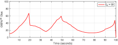
(c) Smoothing (window size = 20)

Figure 4: OSPA⁽²⁾ (with 10 scans) performance from GLMB filtering and GLMB smoothing with window sizes 5 and 20.

(a) Filtering

(b) Smoothing (window size = 5)

(c) Smoothing (window size = 20)

Figure 5: Comparison of estimated cardinality from GLMB filtering and GLMB smoothing with window sizes 5 and 20.

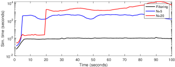
Figure 6: Run time comparison of GLMB filtering and GLMB smoothing with window sizes 5 and 20.

IV Results

A simulation was performed to evaluate performance of the proposed moving window based smoother. Births, deaths and movements of a set of $12$ objects are simulated in a 2D surveillance area of $[-1000,1000]\times[-1000,1000]m^{2}$ over $100$ timesteps. The births occur at timesteps $1$, $20$ and $50$ (respectively $4$, $4$ and $4$), and the objects born at time $1$ die at time $10$, objects born at time $20$ die at time $40$, and objects born at time $50$ die at time $90$. The probability of survival of each object is set to $P_{S}(x^{(\ell)},\ell)=0.95$. The 2D positions of the objects are measured using a sensor that adds noise and measurement cluttter. The probability of detection of the sensor is set to $P_{D}(x^{(\ell)},\ell)=0.3$, and clutter is modeled as a Poisson RFS with the rate of $3$ per scan and points are uniformely distributed over the surveillance region. The objects follow a constant velocity motion model, and the kinematic state of an object is represented by a 4D state vector consisting of 2D position and velocity given by $x_{k}=[p_{x,k},\dot{p}_{x,k},p_{y,k},\dot{p}_{y,k}]$. The single object transition density is modeled by a linear gaussian given by $f_{S,k|k-1}(x_{k+1}^{(\ell)}|x_{k}^{(\ell)})=\mathcal{N}(x_{k+1}^{(\ell)};F_{k}x_{k}^{(\ell)},Q_{k})$ where

$$F_{k}=I_{2}\otimes\left[\begin{array}[]{cc}1&\Delta\\ 0&1\end{array}\right],\hskip 22.76228ptQ_{k}=\sigma_{a}^{2}I_{2}\otimes\left[\begin{array}[]{cc}\frac{\Delta^{4}}{4}&\frac{\Delta^{3}}{2}\\ \frac{\Delta^{3}}{2}&\Delta^{2}\end{array}\right],$$

$I_{2}$ is the $2\times 2$ identity matrix, $\Delta=1s$ is the sampling time, $\sigma_{a}=1\ m/s^{2}$, and $\otimes$ denotes the matrix outer product. Birth objects are modeled by a Labeled Multi-Bernoulli (LMB) Process having birth and spatial distribution parameters $\{r_{B,k}(\ell_{i}),p_{B,k}^{(i)}(\ell_{i})\}_{i=1}^{4}$, where $\ell_{i}=(k,i)\in\mathbb{B}_{k}$, $r_{B,k}(\ell_{i})=0.03$, $p_{B,k}^{(i)}(x^{(\ell_{i})},\ell_{i})=\mathcal{N}(x^{(\ell_{i})};m_{B,k}^{(i)},Q_{B,k})$, $m_{B,k}^{(1)}=\ (500,0,500,0)^{T},$ $m_{B,k}^{(2)}=\ (-500,0,500,0)^{T},$ $m_{B,k}^{(3)}=\ (-500,0,-500,0)^{T},$ $m_{B,k}^{(4)}=\ (500,0,-500,0)^{T},$ and $Q_{B,k}=\ \mathrm{diag}([15,15,15,15]^{2}).$ The measurements are modeled by a linear gaussian likelihood function of the form $g_{k}(z_{k}|x_{k}^{(\ell)})=\mathcal{N}(z_{k};H_{k}x_{k}^{(\ell)},R_{k})$, where $R_{k}=\mathrm{diag}([30,30]^{2})$ and measurements are of the form $z_{k}^{(v)}=[z_{x,k}^{(v)},z_{y,k}^{(v)}]^{T}$.

Algorithm 2 is executed with window sizes $5$ and $20$, and compare estimated tracks, cardinality, OSPA [27], OSPA⁽²⁾ [2] with the GLMB filter. Fig. 2 compares the estimated tracks. The OSPA and OSPA⁽²⁾ matrics are compared in Fig. 3 and Fig. 4, and it can be seen that smoothing with window sizes 5 and 20 produce smaller OSPA and OSPA⁽²⁾ errors than filtering, and increasing the windows size results in smaller OSPA and OSPA⁽²⁾ errors. The cardinality is compared in Fig. 5. The actual time (in seconds) taken to simulate each timestep is compared in Fig. 6. It is clear that the larger the window size better the performance is, and a smaller window size with an acceptable running time can improve the results over filtering.

V Conclusions

In this paper we introduce an approximate, practical approach to the multi-scan multi-target tracking problem using a moving window based technique. We adopt the recent GLMB smoother based on the Gibbs sampling based posterior truncation, and propose to recursively propagate the multi-target posterior using the most recent $N$ scans, by linking the measurement association maps using labels. The efficicacy of the approach is demonstrated using a muli-target tracking simulation with $100$ timesteps.

VI Acknowledgement

This work was supported by the Defence Science Centre Collaborative Research Grant (in 2020).

References

- [1] Y. Bar-Shalom, P.K. Willett and X. Tian, Tracking and Data Fusion: A Handbook of Algorithms: YBS Publishing, 2011.
- [2] M. Beard, B.-T. Vo, and B.-N. Vo, “A Solution for Large-Scale Multi-Object Tracking,” IEEE Trans. Signal Processing, 68:2754–2769, 2020.
- [3] M. Beard, et. al, "Void Probabilities and Cauchy-Schwarz Divergence for Generalized Labeled Multi-Bernoulli Models," IEEE Trans. Signal Processing, 65(19):5047–5061, 2017.
- [4] S.S. Blackman and R. Popoli, Design and Analysis of Modern Tracking Systems: Artech House, 1999.
- [5] D. Bryant et. al., "A Generalized Labeled Multi-Bernoulli Filter with Object Spawning," IEEE Trans. Signal Processing, 66(23):6177–6189, 2018.
- [6] H. Cai, et. al., “Multisensor tasking using analytical Rényi divergence in labeled multi-Bernoulli filtering,” J. Guidance, Control, & Dynamics, 42(9):2078–2085, 2019.
- [7] C.P. Robert and G. Casella, Monte Carlo Statistical Methods, 2nd ed. Springer Texts in Statistics, 2004.
- [8] C.-T. Do and H. Van Nguyen, “Tracking multiple targets from multistatic Doppler radar with unknown probability of detection,” Sensors, 19(7) 2019.
- [9] C. Fantacci et.al. “Robust fusion for multisensor multiobject tracking,” IEEE Signal Process. Lett., 25(5):640–644, 2018.
- [10] J. A. Gaebler, P. Axelrad, and P. W. Schumacher, “Cubesat cluster deployment track initiation via a radar admissible region birth model,” J. Guidance, Control &Dynamics, 43(10):1927–1934, 2020.
- [11] J. A. Gaebler and P. Axelrad, “Identity management of clustered satellites with a generalized labeled multi-Bernoulli filter,” J. Guidance, Control, & Dynamics, 43(11):2046–2057, 2020.
- [12] A. K. Gostar, et. al., “Interactive multiple-target tracking via labeled multi-Bernoulli filters,” in Int. Proc. Conf. Control, Aut. & Info. Sciences, pp. 1–6, 2019.
- [13] A. K. Gostar, et. al. “Centralized cooperative sensor fusion for dynamic sensor network with limited field-of-view via labeled multi-Bernoulli filter,” IEEE Trans. Signal Process., vol. 69, pp. 878–891, 2021.
- [14] D.Y. Kim, et. al. “A Labeled Random Finite Set Online Multi-Object Tracker for Video Data,” Pattern Recognition, 90(6):377-389, 2019.
- [15] S. Li, et. al. “Robust distributed fusion with labeled random finite sets,” IEEE Trans. Signal Process., vol. 66, no. 2, pp. 278–293, 2018.
- [16] S. Li, W. Yi, R. Hoseinnezhad, B. Wang, and L. Kong, “Multiobject tracking for generic observation model using labeled random finite sets,” IEEE Trans. Signal Process., vol. 66, no. 2, pp. 368–383, 2018.
- [17] R. Mahler, “Multitarget Bayes filtering via first-order multitarget moments,” IEEE Trans. Aerosp. Electron. Syst., vol. 39(4):1152–1178, 2003.
- [18] R. Mahler, Statistical Multisource-Multitarget Information Fusion: Artech House, 2007.
- [19] R. Mahler, Advances in Statistical Multisource-Multitarget Information Fusion: Artech House, 2014.
- [20] D. Moratuwage, M. Adams, and F. Inostroza, “δ-generalised labelled multi-Bernoulli simultaneous localisation and mapping,” in Proc. Int. Conf. Control, Aut. & Info. Sciences, pp. 175–182, 2018.
- [21] D. Moratuwage, M. Adams, F. Inostroza, “δ-generalized labeled multi-bernoulli simultaneous localization and mapping with an optimal kernel-based particle filtering approach,” Sensors,19(10), 2019.
- [22] H.V. Nguyen, et. al., "Online UAV Path Planning for Joint Detection and Tracking of Multiple Radio-tagged Objects," IEEE Trans. Signal Processing, 67(20):5365–5379, 2019.
- [23] H.V. Nguyen, et. al., “Multi-objective multi-agent planning for jointly discovering and tracking mobile objects,” in Proc. AAAI Conference on Artificial Intelligence, 34(05):7227–7235, April, 2020.
- [24] T. T. D. Nguyen, et. al., “Tracking Cells and their Lineages via Labeled Random Finite Sets,” IEEE Trans. Signal Processing, 69:5611-5626, 2021.
- [25] J. Ong, et.al., “A Bayesian filter for multi-view 3D multi-object tracking with occlusion handling,” IEEE Trans. Pattern Analysis & Machine Intelligence, 44(5):2246-2263, 2022.
- [26] F. Papi, et. al. “Generalized labeled multi-Bernoulli approximation of multi-object densities,” IEEE Trans. Signal Process., 63(20):5487–5497, 2015.
- [27] D. Schumacher, B.-T. Vo, and B.-N. Vo, “A consistent metric for performance evaluation of multi-object filters,” IEEE Trans. Signal Process., 56(8):3447–3457, 2008.
- [28] B.-N. Vo, B.-T. Vo and R. Mahler, "Close form solutions to Forward-Backward Smoothing," EEE Trans. Signal Process., 60(1):2-17, 2012.
- [29] B.-N. Vo and B.-T. Vo, “Labeled Random Finite Sets and Multi-Object Conjugate Priors,” IEEE Trans. Signal Processing, 61(13):3460-3475, 2013.
- [30] B.-N. Vo, B.-T. Vo, and D. Phung, “Labeled random finite sets and the Bayes multitarget tracking filter,” IEEE Trans. Signal Processing, 62(24):6554–6567, 2014.
- [31] B.-N Vo, B.-T. Vo, and H.G. Hoang, “An Efficient Implementation of the Generalized Labeled Multi-Bernoulli Filter,” EEE Trans. Signal Processing, 65(8):1975-1987, 2017.
- [32] B.-N. Vo, B.-T. Vo, and M. Beard, “Multi-Sensor Multi-Object Tracking with the Generalized Labeled Multi-Bernoulli Filter,” IEEE Trans. Signal Processing, 67(23):5952–5967, 2019.
- [33] B.-N. Vo, and B.-T. Vo. “A Multi-Scan Labeled Random Finite Set Model for Multi-object State Estimation,” EEE Trans. Signal Process., 67(19):4948–4963, 2019. arXiv:1805.10038 [stat.CO].
- [34] B. Wei and B. Nener, “Distributed space debris tracking with consensus labeled random finite set filtering,” Sensors, vol. 18, no. 9, 2018.
- [35] B. Wei and B. Nener, “Multi-sensor space debris tracking for space situational awareness with labeled random finite sets,” IEEE Access, vol. 7, pp. 36991–37003, 2019.
- [36] Y. Zhu, S. Liang, M. Gong, and J. Yan, “Decomposed POMDP optimization-based sensor management for multi-target tracking in passive multi-sensor systems.” IEEE Sensors Journal, 22(4):3565-3578, 2022.
- [37] Y. Zhu, M. Mallick, S. Liang, and J.K. Yan, “Generalized Labeled Multi-Bernoulli Multi-Target Tracking with Doppler-Only Measurements”, Remote Sensing, 14(13), 2022.