Don’t Waste Data: Transfer Learning to Leverage All Data for Machine-Learnt Climate Model Emulation

Abstract

How can we learn from all available data when training machine-learnt climate models, without incurring any extra cost at simulation time? Typically, the training data comprises coarse-grained high-resolution data. But only keeping this coarse-grained data means the rest of the high-resolution data is thrown out. We use a transfer learning approach, which can be applied to a range of machine learning models, to leverage all the high-resolution data. We use three chaotic systems to show it stabilises training, gives improved generalisation performance and results in better forecasting skill. Our code is at https://github.com/raghul-parthipan/dont_waste_data.

1 Introduction

Accurate weather and climate models are key to climate science and decision-making. Often we have a high-resolution physics-based model which we trust, and want to use that to create a lower-cost (lower-resolution) emulator of similar accuracy. There has been much work using machine learning (ML) to learn such models from data [1, 2, 3, 4, 5, 6, 7, 8, 9, 10, 11, 12, 13, 14], due to the difficulty in manually specifying them.

The naive approach is to use coarse-grained high-resolution model data as training data. The high-resolution data is averaged onto the lower-resolution grid and treated as source data. The goal is to match the evolution of the coarse-grained high-resolution model using the lower-resolution one. Such procedures have been used successfully [2, 3, 8, 12, 15, 16]. This has several benefits over using observations, including excellent spatio-temporal coverage. But it has a key downside — the averaging procedure means much high-resolution data is thrown away.

Our novelty is showing that climate model emulation can be framed as a transfer learning task. We can do better by using all of the high-resolution data as an auxiliary task to help learn the low-resolution emulator. And we can do this without any further cost at simulation time. As far as we know, this has not yet been reported in the climate literature. This results in improved generalization performance and forecasting ability, and we demonstrate this on three chaotic dynamical systems.

Related Work.

Transfer learning (TL) has been successfully used for fine-tuning models, including sequence models, in various domains such as natural language processing (NLP) and image classification. There are various methods used such as (1) fine-tuning on an auxiliary task and then the target task [17, 18, 19]; (2) multi-task learning, where fine-tuning is done on the target task and one or more auxiliary tasks simultaneously [20, 21, 22, 23, 24, 25, 26]; and mixtures of the two. Our approach is most similar to the first one. However, our models are not pre-trained as is standard in NLP. Despite this, we show our approach remains successful.

Climate Impact.

A major source of inaccuracies in weather and climate models arises from ‘unresolved’ processes (such as those relating to convection and clouds) [27, 28, 29, 30, 31, 32]. These occur at scales smaller than the resolution of the climate model but have key effects on the overall climate. For example, most of the variability in how much global surface temperatures increase after $\textrm{CO}{{}_{2}}$ concentrations double is due to the representation of clouds [27, 29, 33]. There will always be processes too costly to be explicitly resolved by our current operational models.

The standard approach to deal with these unresolved processes is to model their effects as a function of the resolved ones. This is known as ‘parameterization’ and there is much ML work on this [1, 2, 3, 4, 5, 6, 7, 8, 9, 10, 11, 12, 13, 14]. We propose that by using all available high-resolution data, better ML parameterization schemes and therefore better climate models can be created.

2 Methods

Our approach is a two-step process: first, we train our model on the high-resolution data, and second, we fine-tune it on the low-resolution (target) data.

We denote the low-resolution data at time $t$ as $\mathbf{X}_{t}\in\mathbb{R}^{d}$. The goal is to create a sequence model for the evolution of $\mathbf{X}_{t}$ through time, whilst only tracking $\mathbf{X}_{t}$. We denote the high-resolution data at time $t$ as $\mathbf{Y}_{t}\in\mathbb{R}^{dm}$. In parameterization, $\mathbf{X}_{t}$ is often a temporal and/or spatial averaging of $\mathbf{Y}_{t}$. We wish to use $\mathbf{Y}_{t}$ to learn a better model of $\mathbf{X}_{t}$.

A range of ML models for sequences may be used, but we suggest they should contain both shared and task-specific layers.

We first model $\mathbf{Y}_{t}$, training in the standard teacher-forcing way for ML sequence models. We use the framework of probability, and so train by maximising the log-likelihood of $\mathbf{Y}_{t}$, $\log\mathrm{Pr}(\mathbf{y}_{1},\mathbf{y}_{2},...,\mathbf{y}_{n})$. Informally, the likelihood measures how likely $\mathbf{Y}_{t}$ is to be generated by our sequence model. Next, the weights of the shared layers are frozen and the weights of the target-specific layers are trained to model the low-resolution training data, $\mathbf{X}_{t}$. Again, under the probability framework, this means maximising the log-likelihood of $\mathbf{X}_{t}$, $\log\mathrm{Pr}(\mathbf{x}_{1},\mathbf{x}_{2},...,\mathbf{x}_{n})$.

2.1 RNN Model

We use the recurrent neural network (RNN) to demonstrate our approach (though it is not limited to the RNN). RNNs are well-suited to parameterization tasks [4, 5, 11, 14, 34] as they only track a summary representation of the system history, reducing simulation cost. This is unlike the Transformer [35] which requires a slice of the actual history of $\mathbf{X}_{t}$.

For our RNN, the hidden state is shared and its evolution is described by $\mathbf{h}_{t+1}=f_{\theta}(\mathbf{h}_{t},\mathbf{X}_{t})$ where $\mathbf{h}_{t}\in\mathbb{R}^{H}$ and $f_{\theta}$ is a GRU cell [36]. We model the low-resolution data as

$$\mathbf{X}_{t+1}=\mathbf{X}_{t}+g_{\theta}(\mathbf{h}_{t+1})+\sigma\mathbf{z}_{t}$$ (1)

and the high-resolution as

$$\mathbf{Y}_{t+1}=\mathbf{Y}_{t}+j_{\theta}(\mathbf{h}_{t+1})+\rho\mathbf{w}_{t}$$ (2)

where the functions $g_{\theta}$ and $j_{\theta}$ are represented by task-specific dense layers, $\mathbf{z}_{t}\sim\mathcal{N}(0,I)$ and $\mathbf{w}_{t}\sim\mathcal{N}(0,I)$. The learnable parameters are the neural network weights $\theta$ and the noise terms $\sigma\in\mathbb{R}^{1}$ and $\rho\in\mathbb{R}^{1}$. Further details are in Appendix A.

2.2 Evaluation

We use hold-out log-likelihood to assess generalization to unseen data, a standard probabilistic approach in ML. The models were trained with 15 different random seed initializations to ensure the differences in the results were due to our approach as opposed to a quirk of a particular random seed. This is used to generate 95% confidence intervals. Likelihood is not easily interpretable nor the end-goal of operational climate models. Ultimately we want to use weather and climate models to make forecasts, and it is common to measure forecast skill with error and spread [6, 37] so this is also done for evaluation.

In each case we compare to the baseline of no transfer learning i.e. training solely on $\mathbf{X}_{t}$. The goal of our evaluation is to compare our approach against the baseline; it is not to assess if we have created the best model for a particular system.

3 Results and Discussion

We demonstrate our approach on three chaotic dynamical systems: (1) Kuramoto-Sivashinsky (KS), (2) Brusselator, and (3) Lorenz 96 (L96). These systems have been used extensively in emulation studies [6, 11, 38, 39, 40, 41, 42, 43] and are well-suited here as we can mimic the separation of low- and high-resolution data. This is as follows: for the KS, $\mathbf{X}_{t}$ is a temporal and spatial averaging of $\mathbf{Y}_{t}$ across 5 time-steps and 5 spatial steps; for the Brusselator, it is as for the KS but the averaging is over 5 time-steps and 8 spatial steps; and for the L96, the model itself makes a separation between low- and high-resolution variables. Further details on each system are in Appendix B.

For all three systems, the initial high-resolution training lasted 20 epochs. The number of epochs for the subsequent low-resolution fine-tuning was selected to ensure the models were trained enough to allow convergence if possible. This was 200 (KS), 400 (Brusselator) and 250 (L96). The training data consisted of sequences with the following number of points: 10,000 (KS), 600 (Brusselator) and 400 (L96). For each of the 15 randomly initialized models, early stopping was used during training on a validation sequence of 10,000 points.

3.1 Hold-out Log-Likelihood

The hold-out log-likelihood is shown in Table 1. In all cases, a 30,000-length sequence is used as the hold-out set. A buffer between the training, validation and hold-sets is kept to ensure temporal independence.

Our transfer learning approach improves on the baseline in all cases. Moreover, it gives far tighter confidence intervals over the average hold-out log-likelihoods. This suggests the approach helps better optima be reached in parameter space, improves generalisation, and reduces sensitivity to the initial random seed. Practically, the latter means reduced training costs as you do not need to run many randomly initialized training runs to account for the random seed’s effect.

The improved generalisation performance of our approach is also seen in what happens when early stopping is removed. Without it, our approach continues to fare well — with continued training, the validation loss is stable; however, the no-TL approach begins to overfit and early stopping is required to select a reasonable model.

Table 1: Log-likelihoods on hold-out set. Higher is better. ‘Max’ is the hold-out log-likelihood of the model with the greatest validation log-likelihood. ‘Average’ is the average of hold-out log-likelihoods for the 15 initializations. A 95% confidence interval is included.

System	Transfer Learning		No Transfer Learning
	Max	Average	Max	Average
KS	93.09	91.73 $\pm$0.62	71.52	37.74 $\pm$16.50
Brusselator	452.27	384.64 $\pm$27.41	-1433.95	-555.40 $\pm$486.39
L96	13.09	11.51 $\pm$ 0.64	6.78	4.37 $\pm$ 1.07

3.2 Forecasting Skill

Forecasts were made using the ‘Max’ model in Table 1 in the following way. $M=500$ initial conditions were randomly selected from data separate to the training set, and an ensemble of $N=40$ forecasts each 500 time-steps long were produced from each initial condition. Figure 1 shows (1) the error (intuitively, how far the ensemble mean is from the truth), $\sqrt{\frac{1}{Md}\sum_{m=1}^{M}\sum_{i=1}^{d}\big{(}X_{m,i}^{O}(t)-\overline{X_{m,i}^{\text{sample}}(t)}\big{)}^{2}}$, where $X_{m,i}^{O}(t)$ is the $i^{\text{th}}$ dimension of the observed state at time $t$ for the $m^{\text{th}}$ initial condition, and $\overline{X_{m,i}^{\text{sample}}(t)}$ is the ensemble mean forecast at time $t$; and (2) the spread of the ensemble members, $\sqrt{\frac{1}{MNd}\sum_{m=1}^{M}\sum_{n=1}^{N}\sum_{i=1}^{d}\big{(}X_{m,n,i}(t)-\overline{X_{m,i}^{\text{sample}}(t)}\big{)}^{2}}$.

Our TL approach results in significantly lower errors across the shown systems. In a perfectly reliable forecast, for large $N$ and $M$ the error should also be equal to the spread [37].The spreads are not well-matched in either approach though.

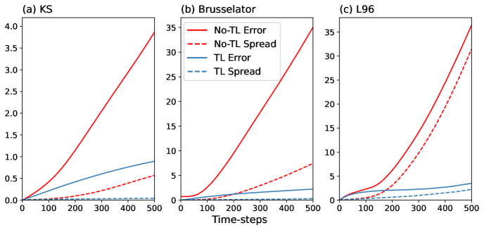
Figure 1: Forecast error and spread. In all cases the TL approach has far lower error.

3.3 Effect of Training Data Size and Sensitivity to Hyperparameters

As the size of the training set increases, the usefulness of the high-resolution data decreases. This is consistent with the TL literature. We found that in these systems, $\frac{\textrm{(\# neural network parameters)}^{0.1}d^{0.5}10^{4}}{\textrm{(training sequence length)}^{1.5}}\lesssim 1$ (where $\mathbf{X}_{t}\in\mathbb{R}^{d}$) was a reasonable indicator for our approach providing less benefit. Importantly, as the training data increases, our approach did not worsen results compared to the baseline, instead just giving similar performance.

Our approach is a form of regularization and should be seen as a complement to other forms such as dropout. Its usefulness depends on the need for regularization. We found that for a range of model complexities and data sizes it remained successful. However, if sufficient regularization was already provided by a simple enough network architecture, our approach provided no further benefit. Similarly, there were cases where increased regularization (more dropout; using our approach) for a particular model complexity could not prevent overfitting. In such cases, more data is often required.

4 Conclusion

By setting up the problem as a transfer learning task, we have shown how to learn from all high-resolution data to create low-resolution emulators. Our approach is a two-step process. It performs particularly well in data-scarce scenarios, acting as a regularizer.

We also tried multi-task learning, where fine-tuning is done on the low- and high-resolution data simultaneously, but it provided no benefit here. However, there may be other set-ups where it does provide value.

There are potentially many helpful auxiliary tasks to use. For example, in operational forecasting models we might have high-resolution data only for specific spatial or temporal regions. Our approach is one way to learn from this. Looking ahead, this now needs testing in such operational models.

Appendix A RNN Architecture

In all cases, the RNN architecture takes the form as shown in the generative model in Figure 2. There is a single GRU layer and it represents the function $f_{\theta}$ from $\mathbf{h}_{t+1}=f_{\theta}(\mathbf{h}_{t},\mathbf{X}_{t})$. The neural network layers mapping $\mathbf{h}_{t}$ to $\mathbf{Y}_{t}$ represent $j_{\theta}$ in equation 2, and those mapping $\mathbf{h}_{t}$ to $\mathbf{X}_{t}$ represent $g_{\theta}$ in equation 1. The dropout rate is 0.3 in all cases. All models were trained using truncated back propagation through time on sequences of length 100 time steps with a batch size of 32 using Adam [44]. The number of nodes in each layer and the learning rates used are given in Table 2.

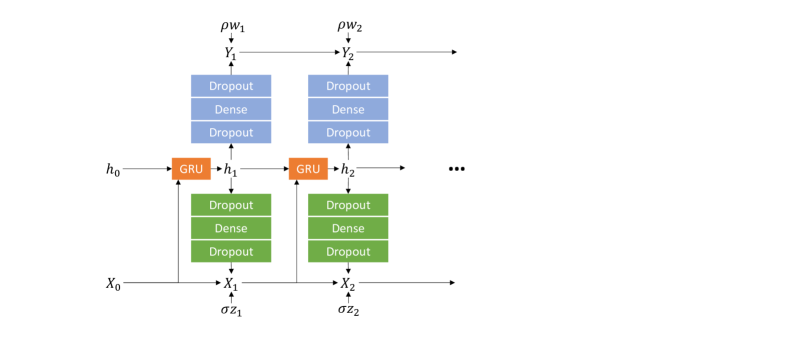
Figure 2: RNN graphical model showing how each $\mathbf{X}_{t}$ is generated. $\mathbf{z}_{t}$ and $\mathbf{w}_{t}$ are exogenous noise. $\mathbf{X}_{t}$ is not a function of $\mathbf{Y}_{t-1}$ so it is not necessary to track $\mathbf{Y}_{t}$ at simulation time.

Table 2: Hyperparameters used for each experiment.

Experiment	GRU units	Dense units for $\mathbf{X}_{t}$	Dense units for $\mathbf{Y}_{t}$	Learning rate
KS	8	8	16	0.001
Brusselator	8	64	64	0.0003
L96	32	32	4	0.001

Appendix B Details on Dynamical Systems

B.1 Kuramoto-Sivashinsky

The Kuramoto-Sivashinsky equation [45, 46] models diffusive-thermal instabilities in a laminar flame front. The one-dimensional KS equation is given by the PDE

$$\frac{\partial{u}}{\partial{t}}=-\nu\frac{\partial^{4}{u}}{\partial{x^{4}}}-\frac{\partial^{2}{u}}{\partial{x^{2}}}-u\frac{\partial{u}}{\partial{x}}$$ (3)

on the domain $\Omega=[0,L]$ with periodic boundary conditions $u(0,t)=u(L,t)$ and $\nu=1$. The case $L=22$ is used here as it results in a chaotic attractor. Equation 3 is discretized with a grid of 100 points and solved with a time-step of $\delta t=0.00005$ using the py-pde package [47]. The data are subsampled to $\Delta t=0.002$ to create $\mathbf{Y}_{t}$. The first 10,000 steps are discarded.

B.2 Brusselator

The Brusselator [48] is a model for an autocatalytic chemical reaction. The two-dimensional Brusselator equation is given by the PDEs

$$\frac{\partial{u}}{\partial{t}} =D_{0}\nabla^{2}u+a-(1+b)u+vu^{2}$$ (4)

$$\frac{\partial{v}}{\partial{t}} =D_{1}\nabla^{2}v+bu-vu^{2}$$ (5)

on the domain $\Omega=[[0,64],[0,64]]$ with $D_{0}=1,D_{1}=0.1,a=1$ and $b=3$. The parameters lead to an unstable regime. Here, $D_{0}=1$ and $D_{1}=0.1$ are diffusivities and $a$ and $b$ are related to reaction rates. Equations 4–5 are discretized on a unit grid and solved with a time-step of $\delta t=0.0002$ using the py-pde package [47]. The data are subsampled to $\Delta t=0.002$ to create $\mathbf{Y}_{t}$. The first 10,000 steps are discarded.

B.3 Lorenz 96

The Lorenz 96 is a model for atmospheric circulation [49]. We use the two-tier version which consists of two scales of variables: a large, low-frequency variable, $X_{k}$, coupled to small, high-frequency variables, $Y_{j,k}$. These evolve as follows

$$\frac{dX_{k}}{dt} =-X_{k-1}(X_{k-2}-X_{k+1})-X_{k}+F-\frac{hc}{b}\sum_{j=J(k-1)+1}^{kJ}Y_{j}$$ (6)

$$\frac{dY_{j,k}}{dt} =-cbY_{j+1,k}(Y_{j+2,k}-Y_{j-1,k})-\,cY_{j,k}-\frac{hc}{b}X_{k}$$ (7)

where in our experiments, the number of $X_{k}$ variables is $K=8$, and the number of $Y_{j,k}$ variables per $X_{k}$ is $J=32$. The value of the constants are set to $h=1,\>b=10$ and $\>c=10$. These indicate that the fast variable evolves ten times faster than the slow variable and has one-tenth the amplitude. The forcing term, $F$, is set to $F=20$. Equations 6–7 are solved using a fourth-order Runge-Kutta scheme with a time-step of $\delta t=0.001$. The data are subsampled to $\Delta t=0.005$ to create $\mathbf{X}_{t}$ and $\mathbf{Y}_{t}$. The first 10,000 steps are discarded.

References

- [1] Troy Arcomano, Istvan Szunyogh, Alexander Wikner, Jaideep Pathak, Brian R Hunt, and Edward Ott. A hybrid approach to atmospheric modeling that combines machine learning with a physics-based numerical model. Journal of Advances in Modeling Earth Systems, 14(3):e2021MS002712, 2022.
- [2] Noah D Brenowitz and Christopher S Bretherton. Prognostic validation of a neural network unified physics parameterization. Geophysical Research Letters, 45(12):6289–6298, 2018.
- [3] Noah D Brenowitz and Christopher S Bretherton. Spatially extended tests of a neural network parametrization trained by coarse-graining. Journal of Advances in Modeling Earth Systems, 11(8):2728–2744, 2019.
- [4] Ashesh Chattopadhyay, Pedram Hassanzadeh, and Devika Subramanian. Data-driven predictions of a multiscale lorenz 96 chaotic system using machine-learning methods: reservoir computing, artificial neural network, and long short-term memory network. Nonlinear Processes in Geophysics, 27(3):373–389, 2020.
- [5] Ashesh Chattopadhyay, Adam Subel, and Pedram Hassanzadeh. Data-driven super-parameterization using deep learning: Experimentation with multiscale lorenz 96 systems and transfer learning. Journal of Advances in Modeling Earth Systems, 12(11):e2020MS002084, 2020.
- [6] David John Gagne, Hannah M Christensen, Aneesh C Subramanian, and Adam H Monahan. Machine learning for stochastic parameterization: Generative adversarial networks in the lorenz’96 model. Journal of Advances in Modeling Earth Systems, 12(3):e2019MS001896, 2020.
- [7] Pierre Gentine, Mike Pritchard, Stephan Rasp, Gael Reinaudi, and Galen Yacalis. Could machine learning break the convection parameterization deadlock? Geophysical Research Letters, 45(11):5742–5751, 2018.
- [8] Vladimir M Krasnopolsky, Michael S Fox-Rabinovitz, and Alexei A Belochitski. Using ensemble of neural networks to learn stochastic convection parameterizations for climate and numerical weather prediction models from data simulated by a cloud resolving model. Advances in Artificial Neural Systems, 2013, 2013.
- [9] Paul A O’Gorman and John G Dwyer. Using machine learning to parameterize moist convection: Potential for modeling of climate, climate change, and extreme events. Journal of Advances in Modeling Earth Systems, 10(10):2548–2563, 2018.
- [10] Stephan Rasp, Michael S Pritchard, and Pierre Gentine. Deep learning to represent subgrid processes in climate models. Proceedings of the National Academy of Sciences, 115(39):9684–9689, 2018.
- [11] Pantelis R Vlachas, Georgios Arampatzis, Caroline Uhler, and Petros Koumoutsakos. Multiscale simulations of complex systems by learning their effective dynamics. Nature Machine Intelligence, 4(4):359–366, 2022.
- [12] Janni Yuval and Paul A O’Gorman. Stable machine-learning parameterization of subgrid processes for climate modeling at a range of resolutions. Nature communications, 11(1):1–10, 2020.
- [13] Janni Yuval, Paul A O’Gorman, and Chris N Hill. Use of neural networks for stable, accurate and physically consistent parameterization of subgrid atmospheric processes with good performance at reduced precision. Geophysical Research Letters, 48(6):e2020GL091363, 2021.
- [14] Pantelis R Vlachas, Wonmin Byeon, Zhong Y Wan, Themistoklis P Sapsis, and Petros Koumoutsakos. Data-driven forecasting of high-dimensional chaotic systems with long short-term memory networks. Proceedings of the Royal Society A: Mathematical, Physical and Engineering Sciences, 474(2213):20170844, 2018.
- [15] Hannah M Christensen. Constraining stochastic parametrisation schemes using high-resolution simulations. Quarterly Journal of the Royal Meteorological Society, 146(727):938–962, 2020.
- [16] Thomas Bolton and Laure Zanna. Applications of deep learning to ocean data inference and subgrid parameterization. Journal of Advances in Modeling Earth Systems, 11(1):376–399, 2019.
- [17] Jason Phang, Thibault Févry, and Samuel R Bowman. Sentence encoders on stilts: Supplementary training on intermediate labeled-data tasks. arXiv preprint arXiv:1811.01088, 2018.
- [18] Ross Girshick, Jeff Donahue, Trevor Darrell, and Jitendra Malik. Rich feature hierarchies for accurate object detection and semantic segmentation. In Proceedings of the IEEE conference on computer vision and pattern recognition, pages 580–587, 2014.
- [19] Yin Cui, Yang Song, Chen Sun, Andrew Howard, and Serge Belongie. Large scale fine-grained categorization and domain-specific transfer learning. In Proceedings of the IEEE conference on computer vision and pattern recognition, pages 4109–4118, 2018.
- [20] Joachim Bingel and Anders Søgaard. Identifying beneficial task relations for multi-task learning in deep neural networks. arXiv preprint arXiv:1702.08303, 2017.
- [21] Soravit Changpinyo, Hexiang Hu, and Fei Sha. Multi-task learning for sequence tagging: An empirical study. arXiv preprint arXiv:1808.04151, 2018.
- [22] Minh-Thang Luong, Quoc V Le, Ilya Sutskever, Oriol Vinyals, and Lukasz Kaiser. Multi-task sequence to sequence learning. arXiv preprint arXiv:1511.06114, 2015.
- [23] Yifan Peng, Qingyu Chen, and Zhiyong Lu. An empirical study of multi-task learning on bert for biomedical text mining. arXiv preprint arXiv:2005.02799, 2020.
- [24] Ronan Collobert and Jason Weston. A unified architecture for natural language processing: Deep neural networks with multitask learning. In Proceedings of the 25th international conference on Machine learning, pages 160–167, 2008.
- [25] Pengfei Liu, Xipeng Qiu, and Xuanjing Huang. Recurrent neural network for text classification with multi-task learning. arXiv preprint arXiv:1605.05101, 2016.
- [26] Weifeng Ge and Yizhou Yu. Borrowing treasures from the wealthy: Deep transfer learning through selective joint fine-tuning. In Proceedings of the IEEE conference on computer vision and pattern recognition, pages 1086–1095, 2017.
- [27] Tapio Schneider, João Teixeira, Christopher S Bretherton, Florent Brient, Kyle G Pressel, Christoph Schär, and A Pier Siebesma. Climate goals and computing the future of clouds. Nature Climate Change, 7(1):3–5, 2017.
- [28] Mark J Webb, F Hugo Lambert, and Jonathan M Gregory. Origins of differences in climate sensitivity, forcing and feedback in climate models. Climate Dynamics, 40(3):677–707, 2013.
- [29] Steven C Sherwood, Sandrine Bony, and Jean-Louis Dufresne. Spread in model climate sensitivity traced to atmospheric convective mixing. Nature, 505(7481):37–42, 2014.
- [30] Eric M Wilcox and Leo J Donner. The frequency of extreme rain events in satellite rain-rate estimates and an atmospheric general circulation model. Journal of Climate, 20(1):53–69, 2007.
- [31] Paulo Ceppi and Dennis L Hartmann. Clouds and the atmospheric circulation response to warming. Journal of Climate, 29(2):783–799, 2016.
- [32] Chia-Chi Wang, Wei-Liang Lee, Yu-Luen Chen, and Huang-Hsiung Hsu. Processes leading to double intertropical convergence zone bias in cesm1/cam5. Journal of Climate, 28(7):2900–2915, 2015.
- [33] Mark D Zelinka, Timothy A Myers, Daniel T McCoy, Stephen Po-Chedley, Peter M Caldwell, Paulo Ceppi, Stephen A Klein, and Karl E Taylor. Causes of higher climate sensitivity in cmip6 models. Geophysical Research Letters, 47(1):e2019GL085782, 2020.
- [34] Pantelis R Vlachas, Jaideep Pathak, Brian R Hunt, Themistoklis P Sapsis, Michelle Girvan, Edward Ott, and Petros Koumoutsakos. Backpropagation algorithms and reservoir computing in recurrent neural networks for the forecasting of complex spatiotemporal dynamics. Neural Networks, 126:191–217, 2020.
- [35] Ashish Vaswani, Noam Shazeer, Niki Parmar, Jakob Uszkoreit, Llion Jones, Aidan N Gomez, Łukasz Kaiser, and Illia Polosukhin. Attention is all you need. Advances in neural information processing systems, 30, 2017.
- [36] Kyunghyun Cho, Bart Van Merriënboer, Caglar Gulcehre, Dzmitry Bahdanau, Fethi Bougares, Holger Schwenk, and Yoshua Bengio. Learning phrase representations using rnn encoder-decoder for statistical machine translation. arXiv preprint arXiv:1406.1078, 2014.
- [37] Martin Leutbecher and Tim N Palmer. Ensemble forecasting. Journal of computational physics, 227(7):3515–3539, 2008.
- [38] H M Arnold, I M Moroz, and T N Palmer. Stochastic parametrizations and model uncertainty in the lorenz’96 system. Philosophical Transactions of the Royal Society A: Mathematical, Physical and Engineering Sciences, 371(1991):20110479, 2013.
- [39] Daan Crommelin and Eric Vanden-Eijnden. Subgrid-scale parameterization with conditional markov chains. Journal of the Atmospheric Sciences, 65(8):2661–2675, 2008.
- [40] Frank Kwasniok. Data-based stochastic subgrid-scale parametrization: an approach using cluster-weighted modelling. Philosophical Transactions of the Royal Society A: Mathematical, Physical and Engineering Sciences, 370(1962):1061–1086, 2012.
- [41] Stephan Rasp. Coupled online learning as a way to tackle instabilities and biases in neural network parameterizations: general algorithms and lorenz 96 case study (v1. 0). Geoscientific Model Development, 13(5):2185–2196, 2020.
- [42] Jaideep Pathak, Zhixin Lu, Brian R Hunt, Michelle Girvan, and Edward Ott. Using machine learning to replicate chaotic attractors and calculate lyapunov exponents from data. Chaos: An Interdisciplinary Journal of Nonlinear Science, 27(12):121102, 2017.
- [43] Maziar Raissi and George Em Karniadakis. Hidden physics models: Machine learning of nonlinear partial differential equations. Journal of Computational Physics, 357:125–141, 2018.
- [44] Diederik P Kingma and Jimmy Ba. Adam: A method for stochastic optimization. arXiv preprint arXiv:1412.6980, 2014.
- [45] Yoshiki Kuramoto. Diffusion-induced chaos in reaction systems. Progress of Theoretical Physics Supplement, 64:346–367, 1978.
- [46] Gregory I Sivashinsky. Nonlinear analysis of hydrodynamic instability in laminar flames—i. derivation of basic equations. Acta astronautica, 4(11):1177–1206, 1977.
- [47] David Zwicker. py-pde: A python package for solving partial differential equations. Journal of Open Source Software, 5(48):2158, 2020.
- [48] Ilya Prigogine and René Lefever. Symmetry breaking instabilities in dissipative systems. ii. The Journal of Chemical Physics, 48(4):1695–1700, 1968.
- [49] Edward N Lorenz. Predictability: A problem partly solved. In Proc. Seminar on predictability, volume 1, 1996.