Weisfeiler–Lehman goes Dynamic: An Analysis of the Expressive Power of Graph Neural Networks for Attributed and Dynamic Graphs

Abstract

Graph Neural Networks (GNNs) are a large class of relational models for graph processing. Recent theoretical studies on the expressive power of GNNs have focused on two issues. On the one hand, it has been proven that GNNs are as powerful as the Weisfeiler-Lehman test (1-WL) in their ability to distinguish graphs. Moreover, it has been shown that the equivalence enforced by 1-WL equals unfolding equivalence. On the other hand, GNNs turned out to be universal approximators on graphs modulo the constraints enforced by 1-WL/unfolding equivalence. However, these results only apply to Static Undirected Homogeneous Graphs with node attributes. In contrast, real-life applications often involve a variety of graph properties, such as, e.g., dynamics or node and edge attributes. In this paper, we conduct a theoretical analysis of the expressive power of GNNs for these two graph types that are particularly of interest. Dynamic graphs are widely used in modern applications, and its theoretical analysis requires new approaches. The attributed type acts as a standard form for all graph types since it has been shown that all graph types can be transformed without loss to Static Undirected Homogeneous Graphs with attributes on nodes and edges (SAUHG). The study considers generic GNN models and proposes appropriate 1-WL tests for those domains. Then, the results on the expressive power of GNNs are extended by proving that GNNs have the same capability as the 1-WL test in distinguishing dynamic and attributed graphs, the 1-WL equivalence equals unfolding equivalence and that GNNs are universal approximators modulo 1-WL/unfolding equivalence. Moreover, the proof of the approximation capability holds for SAUHGs, which include most of those used in practical applications, and it is constructive in nature allowing to deduce hints on the architecture of GNNs that can achieve the desired accuracy.

Extension of 1-WL test to attributed and dynamic version.

Extension of unfolding trees to attributed and dynamic version.

Proof of equivalence between the (attributed/dynamic) 1-WL and (attributed/dynamic) unfolding tree equivalences.

Extension of the universal approximation theorem to GNNs capable of handling attributted and dynamic graphs.

1 Introduction

Graph data is becoming pervasive in many application domains, such as biology, physics, and social network analysis. Graphs are handy for complex data since they allow us to naturally encode information about entities, their links, and their attributes. In modern applications, several different types of graphs are commonly used, and possibly combined: graphs can be homogeneous or heterogeneous, directed or undirected, have attributes on nodes and/or on edges, be static or dynamic, hyper- or multigraphs. Interestingly, it has recently been shown that Static Attributed Undirected Homogenous Graphs (SAUHGs) with both attributes on nodes and edges can act as a standard form for graph representation, namely that all the common graph types can be transformed into SAUHGs without losing their encoded information [1].

Graph Neural Networks (GNNs) are a large class of relational models that can directly process graphs. Most of these models adopt a computational scheme based on a local aggregation mechanism. The information relevant to a node is stored in a feature vector, which is recursively updated by aggregating the feature vectors of neighboring nodes. After $k$ iterations, the feature vector of a given node $v$ captures the structural information and the local information included within the $v$’s $k$–hop neighborhood. At the end of the iterative process, the node feature vectors can be used to classify/cluster the patterns represented by the nodes or the whole graphs. The study of machine learning for graphs based on neural networks and local aggregation mechanisms started in the 90s with the proposal of some seminal models mainly designed for graph focused applications, including labelling RAAMs [2], recursive neural networks [3, 4], recursive cascade correlation networks [5] and SOM for structure data [6]. In this paper, the Graph Neural Network model [7] is the ancestor of the GNN class and is called Original GNN (OGNN). It is the first GNN designed to face both node/edge and graph-focused tasks. Recently the interest in GNNs has rapidly grown, and a large number of new applications and models have been proposed, including neural networks for graphs [8], Gated Sequence Graph Neural Networks [9], Spectral Networks [10], Graph Convolutional Neural Networks [11], GraphSAGE [12], Graph attention networks [13], and Graph Networks [14]. Another interesting extension of GNNs consisted in the proposal of several new models capable of dealing with dynamic graphs [15], which, for instance, can be used to classify the following graph or the nodes of a sequence of graphs or to predict the insurgence of an edge in a graph.

A great effort has been dedicated to studying the theoretical properties of GNNs and, in particular, their expressive power [16]. A goal of such a study is to define which graphs can be distinguished by a GNN, namely for which input graphs the GNN produces different encodings. In [17], GNNs are proven to be as powerful as the Weisfeiler–Lehman graph isomorphism test (1–WL) [18, 19]. Such an algorithm allows us to test whether two graphs are not isomorphic. The 1–WL algorithm is based on a graph signature that is obtained by assigning a color to each node. The graph coloring is achieved by iterating a local aggregation function. More generally, a hierarchy of algorithms exists, called 1–WL, 2–WL, 3–WL, $\ldots$, whose elements recognize larger and larger classes of graphs. It has been proven that a standard GNN model can simulate the 1–WL test, but it cannot implement higher tests; namely, 3–WL, 4–WL, and so on  [20]. Therefore, the 1–WL test exactly defines the classes of graphs that GNNs can recognize.

Another goal of the research on the expressive power of GNNs is to study GNN approximation capability. Formally, in node-focused applications, a GNN implements a function $\varphi(\mathbf{G},v)\rightarrow\mathbb{R}^{m}$ that takes as input a graph $\mathbf{G}$ and returns an output at each node. Similarly, in graph-focused tasks, a GNN implements a function $\varphi(\mathbf{G})\rightarrow\mathbb{R}^{m}$. In both cases, the study’s objective is to define which classes of functions can be approximated by a GNN model.

Intuitively, existing results suggest, provided that a sufficiently general aggregation function is used, GNNs are universal approximators on graphs except for the following constraint: a GNN must produce the same output $\varphi(\mathbf{G},v)$ on a pair of nodes $v=v_{1},v_{2}$ that can be distinguished neither for their features nor for their neighborhoods. Such a concept can be formally captured in two ways. In most of the recent results, it has been observed that if 1-WL gives the same colors to $v_{1},v_{2}$ then a GNN produces the same outputs on them: this fact can be defined by affirming that $v_{1},v_{2}$ are equivalent according to 1-WL. On the other hand, in [21], which is dedicated to studying the expressive power of the OGNN, the concepts of unfolding trees and unfolding equivalence were adopted. The unfolding tree $\mathbf{T}_{v}$, with root node $v$, is constructed by unrolling the graph starting from that node. Intuitively, $\mathbf{T}_{v}$ exactly describes the information used by the GNN at node $v$. The unfolding equivalence is, in turn, an equivalence relationship defined between nodes having the same unfolding tree: obviously, a GNN cannot distinguish $v_{1},v_{2}$ if they are unfolding equivalent. Interestingly, it has been proven recently [23] that 1-WL and the unfolding equivalences are equal; namely they induce the same relationship between nodes. Thus, 1-WL and the unfolding equivalences can be used interchangeably.

Formally, in [21], it has been proven that OGNNs can approximate in probability, up to any degree of precision, any measurable function $\tau(\mathbf{G},v)\rightarrow\mathbb{R}^{m}$ that respects the unfolding equivalence. Such a result has been recently extended to a large class of GNNs [23] called message passing GNNs, which includes most of the contemporary architectures. Similar results show that the functions implemented by message passing GNNs [17, 24], Linear Graph Neural Networks [24, 25] and Folklore Graph Neural Networks [26] are dense in continuous functions on graphs modulo 1-WL. Interestingly, the most recent results differ for the technique adopted in the proof, which can be based on a partitioning of the input space [23] or Stone-Weierstrass theorem [17, 24, 25, 23]. Such techniques have advantages and disadvantages. Stone-Weierstrass provides a more elegant proof that holds for continuous target functions. Space partitioning provides a constructive proof, allowing us to deduce information about the GNN architectures that can achieve the desired approximation. Moreover, with the latter technique, the proof holds in probability so that it can also be applied to discontinuous target functions.

Despite the availability of the mentioned results on the expressive power of GNNs, their application is still limited to undirected static graphs with attributes on nodes. This is particularly restrictive since modern applications usually involve much more complex data structures, such as heterogeneous, directed, dynamic graphs and multigraphs. Even if, intuitively, one may expect that GNNs can be universal approximators over those extended domains, it is not apparent which GNN architectures can achieve such a universality. So the question is how the definition of the 1-WL test has to be modified to cope with such novel data structures and whether the universal results fail for some particular graph type.

In this paper, we propose a study on the expressive power of GNNs for two exciting domains, namely dynamic graphs and SAUHGs with node and edge attributes. Dynamic graphs are interesting from a practical and a theoretical point of view. They are used in several application domains. Moreover, dynamic GNN models are structurally different from common GNNs, and the results and the methodology required to analyze their expressive power cannot directly be deduced from existing literature. On the other hand, SAUHGs with node and edge attributes are interesting because, as mentioned above, they act as a standard form for several other types of graphs that all can be transformed to SAUGHs [1].

To construct the fundamental theory for both types of domains, appropriate versions of the 1–WL test and the unfolding equivalence are introduced, and we discuss how they are related. Then, we consider generic GNN models that can operate on such domains, and we prove that they are universal approximators modulo the aforementioned 1–WL/unfolding equivalences. More precisely, the main contributions of this paper are as follows.

• We present new versions of the 1–WL test and of the unfolding equivalence that are appropriate for dynamic graphs and SAUHGs with node and edge attributes, and we show that they induce the same equivalences on nodes. Such a result makes it possible to use them interchangeably to study the expressiveness of GNNs.

• We show that generic GNN models for dynamic graphs and SAUHGs with node and edge attributes are capable of approximating, in probability and up to any precision, any measurable function on graphs that respects the 1-WL/unfolding equivalence. The work extends the state-of-the-art results available on approximation capability of GNNs to the two domains, maintaining the best generality and providing information about the architecture achieving the approximation. The result on approximation capability holds for graphs with unconstrained features of reals and measurable target functions. Thus, most of the domains used in practical applications are included. Moreover, the proof is based on space partitioning, which is constructive in nature and allows us to deduce information about the GNN architecture that can achieve the desired approximation. For example, it is shown that, provided that the GNN is endowed with sufficiently general aggregation and combination functions, the approximation is achieved in $r+1$ iterations and that a hidden feature of dimension $1$ is sufficient.

The rest of the paper is organized as follows. Section 2 illustrates the related literature. In section 3, the notation used throughout the paper is described and the main definitions are introduced. In section 4, we introduce the 1–WL test and unfolding equivalences suitable for dynamic graphs and SAUHGs with node and edge attributes and prove that those equivalences are equal. In section 5, the approximation theorems for GNNs on both graph types are presented. Finally, section 6 includes our conclusions and future matter of research. For the sake of simplicity, all of the proofs are collected in the appendix A.

2 Related Work

The Weisfeiler-Lehman test and its variants have been exploited in a wide variety of GNN models since [17] showed that message passing GNNs are as powerful as the 1–WL test. To overcome the limit of 1–WL, a new GNN model is introduced in [27], where node identities are directly injected into the Weisfeiler-Lehman aggregate functions. In [20], the k-WL test has been taken into account to develop a more powerful GNN model, given its greater capability to distinguish non-isomorphic graphs. In [28], a simplicial-wise Weisfeiler-Lehman test is introduced, and it is proven to be strictly more powerful than the 1-WL test and not less powerful than the 3-WL test; a similar test (called cellular WL test) proposed by [29] is proven to be actually more powerful than the simplicial version. Nevertheless, all this proposed tests do not deal with edge-attributed graphs, certainly not with dynamic graphs.

Moreover, the WL test mechanism applied to GNNs has been also studied within the paradigm of unfolding trees ([16],  [30]). However, only recently it has been established an equivalence between the two concepts by [23], and still, it is limited to static graphs without edge attributes.

By a theoretical point of view, several approaches have been carried out to study the approximation and generalization properties of graph neural networks. In [21], the authors proved the universal approximation properties of the original graph neural network model, modulo the unfolding equivalence. Universal approximation is shown for GNNs with random node initialization in [31] while, in [17], GNNs are shown to be able to encode any graph with countable input features. Moreover, the authors of [32] proved that GNNs, provided with a colored local iterative procedure (CLIP), can be universal approximators for functions on graphs with node attributes. The approximation property has been extended also to Folklore Graph Neural Networks in [26] and to Linear Graph Neural Networks and general GNNs in [24, 25], both in the invariant and equivariant case. Recently, the universal approximation theorem has been proved for modern message passing graph neural networks by [23]. Despite the availability of universal approximation theorems for static graphs with node attributes, the theory lacks results about approximation capability of other types of graphs such as dynamic graphs and graphs with attributes on both nodes and edges.
The aim of this paper, is that of extending the results on the expressive power of GNNs for dynamic graphs and SAUHGs with node and edge attributes.

3 Notation and Preliminaries

Before extending the work about the expressive power of GNNs to dynamic and edge attributed graph domains, the mathematical notation and preliminary definitions are given in this chapter. In this paper, only finite graphs are under consideration.

Notation table
$\mathbb{N}$	natural numbers
$\mathbb{N}_{0}$	natural numbers starting at $0$
$\mathbb{R}$	real numbers
$\mathbb{R}^{k}$	$\mathbb{R}$ vector space of dimension $k$
$|a|$	absolute value of a real $a$
$\|\cdot\|$	norm on $\mathbb{R}$
$|M|$	number of elements of a set $M$
$[n],\,n\in\mathbb{N}$	sequence $1,2,\ldots,n$
$[n]_{0},\,n\in\mathbb{N}_{0}$	sequence $0,1,\ldots,n$
$\emptyset$	empty set
$\{\cdot\}$	set
$\{\!|\cdot|\!\}$	multiset, i.e. set allowing
	multiple appearances of entries
|$\cdot$|	sorted multiset
$(x_{i})_{i\in I}$	vector of elements $x_{i}$
	for indices in set $I$
$\wedge$	conjunction
$\cup$	union of two (multi)sets
$\subseteq$	sub(multi)set
$\subsetneq$	proper sub(multi)set
$\times$	factor set of two sets

In [1] it has been proven that several types of graphs can be transformed to SAUGHs with node and edge attributes. Therefore, SAUHGs will be used as a standard form for all the types of graphs defined in the following.

Definition 3.1 (Different Graph Types).

The elementary graphs are defined in [1] as follows.

1. A directed graph (digraph) is a tuple $G=(\mathcal{V},\mathcal{E})$ containing a set of nodes $\mathcal{V}\subset\mathbb{N}$ and a set of directed edges given as tuples $\mathcal{E}\subseteq\mathcal{V}\times\mathcal{V}$. As the set of nodes $\mathcal{V}\subset\mathbb{N}$, each node is provided with an identifier, which is simply the natural number with which is represented; the identifier could be used to create an ordering of the nodes.

2. A (generalized) directed hypergraph is a tuple $G=(\mathcal{V},\mathcal{E})$ with nodes $\mathcal{V}\subset\mathbb{N}$ and hyperedges
   $\mathcal{E}\subseteq\{(\mathsf{x},f_{i})_{i}\mid\mathsf{x}\subseteq\mathcal{V},\,f_{i}\mathbin{:}\mathsf{x}\rightarrow\mathbb{N}_{0}\}$ that include a numbering map $f_{i}$ for the $i$-th edge $(\mathsf{x},f)_{i}$ which indicates the order of the nodes in the (generalized) directed hyperedge.

An elementary graph $G=(\mathcal{V},\mathcal{E})$ is called

1. undirected if the directions of the edges are irrelevant, i.e.,

   • for directed graphs: if $(u,v)\in\mathcal{E}$ whenever $(v,u)\in\mathcal{E}$ for $u,v\in\mathcal{V}$. Then an abbreviation can be the set data type instead of tuples, namely $\mathcal{E}\subseteq\{\{u,v\}\,|\,u,v\in\mathcal{V},u\neq v\}\cup\{\{u\}\mid u\in\mathcal{V}\},$

   • for directed hypergraphs: if $f_{i}\mathbin{:}\mathsf{x}\rightarrow 0$ for all $(\mathsf{x},f_{i})_{i}\in\mathcal{E}$. Abbreviated by $\mathcal{E}\subseteq\{\mathsf{x}\mid\mathsf{x}\subseteq\mathcal{V}\}$.

2. multigraph if it is a multi-edge graph, i.e., the edges $\mathcal{E}$ are defined as a multiset, a multi-node graph, i.e., the node set $\mathcal{V}$ is a multiset, or both.

3. heterogeneous if the nodes or edges can have different types. Mathematically, the type is appended to the nodes and edges. I.e., the node set is determined by $\mathcal{V}\subseteq\mathbb{N}\times\mathcal{S}$ with a node type set $\mathcal{S}$ and thus, a node $(v,s)\in\mathcal{V}$ is given by the node $v$ itself and its type $s$. The edges can be extended by a set $\mathcal{R}$ that describes their types, to $(e,r)\ \forall\,e\in\mathcal{E}\text{ of edge type }r\in\mathcal{R}$.

4. attributed if the nodes $\mathcal{V}$ or edges $\mathcal{E}$ are equipped with node or edge attributes. These attributes are formally given by a node and edge attribute function, respectively, i.e. $\alpha:\mathcal{V}\rightarrow\mathcal{A}$ and $\omega:\mathcal{E}\rightarrow\mathcal{W}$, where $\mathcal{A}$ and $\mathcal{W}$ are arbitrary attribute sets.

Recall that, for any graph type, a graph $G=(\mathcal{V},\mathcal{E})$ is called bounded if $\exists K\in\mathbb{N}$ s.t. $\max\limits_{G\in\mathcal{G}}|G|\leq K$, where $|G|$ is the cardinality of the set $\mathcal{V}$ of nodes.

Since all the graph types introduced in Def. 3.1 are static, but temporal changes (dynamics) play an essential role in learning on graphs representing real-world applications, the dynamic graphs are defined in the following. In particular, the dynamic graph definition here consists of a discrete-time representation.

Definition 3.2 (Dynamic Graph).

Let $T=\{t_{i}\}_{i\in I}\subsetneq\mathbb{R}$ with $I=[0,\ldots,l]\subsetneq\mathbb{N}$ be a set of timestamps. Each timestamp $t_{i}$ can be bijectively identified by its index $i$. Without loss of generality, from now on we refer to the set of timestamps as $I$. Then a (discrete) dynamic graph can be considered as a vector of static graph snapshots, i.e., $G=(G_{t})_{t\in I}$, where $G_{t}=(\mathcal{V}_{t},\mathcal{E}_{t})\;\forall t\in I$. Furthermore,

$$\alpha_{v}(t):=\begin{cases}\alpha(v,t),&\quad v\in\mathcal{V}_{t}\\ \perp,&\quad\text{otherwise}\end{cases}\quad\text{and}\quad$$

$$\omega_{\{u,v\}}(t):=\begin{cases}\omega(\{u,v\},t),&\quad\{u,v\}\in\mathcal{E}_{t}\\ \perp,&\quad\text{otherwise}\end{cases}$$

where $\alpha:\mathcal{V}\times I\rightarrow\mathcal{A}\;\cup\perp$ and $\omega:\mathcal{E}\times I\rightarrow\mathcal{B}\;\cup\perp$ define the vector of dynamic node/edge attributes.

In particular, $\alpha_{v}(t)=\perp$ means that at the timestamp $t$ the node $v$ doesn’t exist. In the same way, $\omega_{\{u,v\}}(t)=\perp$ encodes the absence of the edge at that time. Moreover, let

$$\Omega_{ne_{v}}(t) =\left({\;{\omega_{\{v,x_{1}\}}(t),\ldots,\omega_{\{v,x_{|ne_{v}(t)|}\}}(t)\;}\;}\right)_{t\in I}$$

be the sequence of dynamic edge attributes of the neighborhood corresponding node at each timestamp.

The following definition introduces a static, nodes/edges attributed, undirected and homogeneous graph, called SAUHG. The reason for defining and using it comes from [1]. Here, it is shown, that every graph type is transformable into each other. Thus, it suffices to consider only one graph type in which all graph types are easily transformable to extend the universal approximation theorem to all graph types defined in Def. 3.1 and Def. 3.2.

Definition 3.3 (Static Attributed Undirected Homogeneous Graphs).

$G^{\prime}$ is called static, nodes/edges attributed, undirected, homogeneous graph (SAUHG) if $G^{\prime}=(\mathcal{V},\mathcal{E},\alpha,\omega)$, with $\mathcal{V}\subset\mathbb{N}$ is a finite set of nodes, $\mathcal{E}\subset\{\{u,v\}\mid\forall\,u,v\in\mathcal{V}\}$ is a finite set of edges, and node and edge attributes determined by the mappings ${\alpha\,:\,\mathcal{V}\rightarrow\mathbb{R}^{k},\ \omega\,:\,E\rightarrow\mathbb{R}^{k}}$ that map w.l.o.g. into the same $k$-dimensional attribute space. The domain of SAUGHs will be denoted as $\mathcal{G}$.

There exists a bijective transformation from any arbitrary graph type defined in Def. 3.1 to the SAUHG. They result from concatenating graph type transformations for single graph properties from [1]. In particular, a dynamic graph can be transformed into a static one through the makeStatic transformation, which encodes the dynamical behaviour of the graph into a time series of node and edge attributes accordingly.

Next, the definition of a GNN that can handle static node-attributed undirected homogeneous graphs is given from [17]. Here, the node attributes $\alpha_{v}$ of a node $v\in\mathcal{V}$ are used as the initial representation and input to the GNN. The update is executed by an AGGREGATION over the representations of the neighbouring nodes. In the $i$-th layer of the GNN, the nodes hidden representation is encoded in an embedding vector $\bm{h}_{v}$ containing both the local structural information and the node information within the $i$-hop neighborhood. Dependent on the learning problem under consideration, a READOUT function is used to obtain a suitable output $\bm{z}_{v}$. The entire GNN propagation scheme is defined as follows.

Definition 3.4 (Graph Neural Networks).

The GNN propagation scheme in one iteration $i\in J$ for the representation of a node $v$ is defined as

$$\bm{h}_{v}^{i}=\text{COMBINE}^{(i)}\left(\bm{h}_{v}^{(i-1)},\text{AGGREGATE}^{(i)}\left(\{\bm{h}_{u}^{(i-1)}\mid u\in ne_{v}\}\right)\right)$$

The output for a node specific learning problem after the last iteration $l$ is given by

$$\bm{z}_{v}=\text{READOUT}\left(\bm{h}_{v}^{l}\right)$$

using a selected AGGREGATION scheme and a suitable READOUT function and the output for a graph specific learning problem is determined by

$$\bm{z}=\text{READOUT}\left(\{\bm{h}_{v}^{l}\mid v\in\mathcal{V}\}\right).$$

The GNNs expressivity is studied in terms of their capability of distinguishing two non isomorphic graph.

Definition 3.5 (Graph Isomorphism).

Let $G_{1}$ and $G_{2}$ be two static graphs, then $G_{1}=(\mathcal{V}_{1},\mathcal{E}_{1})$ and $G_{2}=(\mathcal{V}_{2},\mathcal{E}_{2})$ are isomorphic to each other $G_{1}\approx G_{2}$, if and only if there exists a bijective function $\phi:\mathcal{V}_{1}\rightarrow\mathcal{V}_{2}$, with

1. $v_{1}\in\mathcal{V}_{1}\;\Longleftrightarrow\;\phi(v_{1})\in\mathcal{V}_{2}\ \quad\forall\;v_{1}\in\mathcal{V}_{1}$,

2. $\{v_{1},v_{2}\}\in\mathcal{E}_{1}\;\Longleftrightarrow\;\{\phi(v_{1}),\phi(v_{2})\}\in\mathcal{E}_{2}\quad\forall\;\{v_{1},v_{2}\}\in\mathcal{E}_{1}$

In case the two graphs are attributed, i.e.  $G_{1}=(\mathcal{V}_{1},\mathcal{E}_{1},\alpha_{1},\omega_{1})$ and $G_{2}=(\mathcal{V}_{2},\mathcal{E}_{2},\alpha_{2},\omega_{2})$, then $G_{1}\approx G_{2}$ if and only if additionally there exist bijective functions $\varphi_{\alpha}:A_{1}\rightarrow A_{2}$ and $\varphi_{\omega}:B_{1}\rightarrow B_{2}$ with $A_{i}:=\text{im}(\alpha_{i})$ and $B_{i}:=\text{im}(\omega_{i})$, $i=1,2$.

1. $\varphi_{\alpha}(v_{1})=\alpha_{2}(\phi(v_{1}))\quad\forall\;v_{1}\in\mathcal{V}_{1}$,

2. $\varphi_{\omega}(\{u_{1},v_{1}\})=\omega_{2}(\phi(u_{1}),\phi(v_{1}))\quad\forall\;\{u_{1},v_{1}\}\in\mathcal{E}_{1}$.

Graph isomorphism (GI) gained prominence in the theory community when it emerged as one of the few natural problems in the complexity class NP that could neither be classified as being hard (NP-complete) nor shown to be solvable with an efficient algorithm (that is, a polynomial-time algorithm) [33]. Indeed it lies in the class NP-Intermidiate. However, in practice, the so-called Weisfeiler-Lehman (WL) test is used to at least recognize non-isomorphic graphs. If the WL test outputs two graphs as isomorphic, the isomorphism is likely but not given for sure.
There are many different extensions of the WL test, e.g., n-dim. WL test, n-dim folklore WL test or set n-dim. WL test [16]. However, introducing all of them is out of the scope of this paper, so in the following we only introduce the 1-WL test, on which all other WL tests are based.

In general, the 1-WL test is based on a graph coloring algorithm. The coloring is applied in parallel on the nodes of the two input graphs and at the end the number of color used per each graph are counted. Then, two graphs are detected as non-isomorphic if these numbers do not coincide, whereas when the numbers are equal, the graphs are possibly isomorphic.

Definition 3.6 (1-WL test).

Let HASH be a bijective function that codes every possible node attribute with a color and $G=(\mathcal{V},\mathcal{E},\alpha)$. Then, the 1-WL test is recursively defined on the graph nodes by

• At iteration $i=0$ the color is set to the hashed node attribute:

  $$o_{v}^{(0)}=\text{HASH}(\alpha_{v})$$

• For any other iteration $i>0$ it holds

  $$o_{v}^{(i)}=\text{HASH}\Bigl{(}\bigl{(}o_{v}^{(i-1)},o_{ne_{v}}^{(i-1)}\bigr{)}\Bigr{)}$$

The algorithm terminates if the number of colors between two iterations does not change, i.e., if

$$|\{o_{v}^{i}\mid v\in\mathcal{V}\}|=|\{o_{v}^{i+1}\mid v\in\mathcal{V}\}|.$$

It is reasonable to define two graphs as equivalent if their node colors result in the same stable position. Formally, this concept leads to the following expression of WL-equivalence.

Definition 3.7 (WL-equivalence).

Let $G_{1}=(\mathcal{V}_{1},\mathcal{E}_{1},\alpha_{1})$ and $G_{2}=(\mathcal{V}_{2},\mathcal{E}_{2},\alpha_{2})$ be two graphs. Then $G_{1}$ and $G_{2}$ are WL-equivalent, noted by $G_{1}\sim_{WL}G_{2}$, if and only if for all nodes $v_{1}\in\mathcal{V}_{1}$ there exists a corresponding node $v_{2}\in\mathcal{V}_{2}$ with $o_{v_{1}}=o_{v_{2}}$.

Note, that in terms of the GNN expressive power, the GNN is as powerful as the WL test if the hidden embedding representation of two graphs is different in case the input graphs are not equal regarding the WL test. However, another way to check the graph isomorphism of two graphs and therefore compare the GNN expressivity is to considers the so-called unfolding trees of all their nodes. An unfolding tree consists of a tree constructed by a breadth-first visit of the graph, starting from a given node. Two graphs are possibly isomorphic if all their unfolding trees are equal. For this purpose, the following two definitions introduce the notion of an unfolding tree and the concept of unfolding tree equivalence.

Definition 3.8 (Unfolding Trees).

The unfolding tree $\bm{F}_{v}^{d}$ in graph $G=(\mathcal{V},\mathcal{E},\alpha)$ of node $v\in\mathcal{V}$ up to depth $d\in\mathbb{N}$ is defined as

$$\bm{F}_{v}^{d}=\begin{cases}Tree(\alpha_{v}),\quad\text{if }d=0\\ Tree\bigl{(}\alpha_{v},\bm{F}^{d-1}_{ne_{v}}\bigr{)}\quad\text{if }d>0\,,\end{cases}$$

where ${Tree(\alpha_{v})}$ is a tree constituted of node $v$ with attribute $\alpha_{v}$. Furthermore, $Tree\bigl{(}\alpha_{v},\bm{F}^{d-1}_{ne_{v}}\bigr{)}$ is the tree with root node $v$ and subtrees $\bm{F}^{d-1}_{ne_{v}}=\{\!|\bm{F}_{u_{1}}^{d-1},\ldots,\bm{F}_{u_{|ne_{v}|}}^{d-1}|\!\}$ with roots in the neighbors of $v$ of depth $d-1$ if $\alpha_{v}\neq\,\perp$ or empty otherwise.

Moreover, the unfolding tree of $v$ determined by $\bm{F}_{v}=\lim_{d\rightarrow\infty}\bm{F}_{v}^{d}$ is obtained by merging all unfolding trees $\bm{F}^{d}_{v}$ of any depth $d$.

Remark 3.9.

Note that in the aforementioned definition the subtrees are given by a multiset. Indeed this is essential since there might be nodes within a graph which induce equal unfolding trees. However, for some applications or graph types, e.g. positional graphs where the neighbourhood of each node is sorted by some given order, it could be necessary to use a sorted multiset.

Analogous to the WL equivalence between two graphs with the new approach of computing the unfolding trees of the nodes of each graph leads to the notion of unfolding equivalence between two graphs which is defined as follows.

Definition 3.10 (Unfolding Tree Equivalence).

Two nodes $u$, $v$ are said to be unfolding equivalent $u\backsim_{ue}v$, if $\mathbf{F}_{u}=\mathbf{F}_{v}$. Moreover,let $G_{1}=(\mathcal{V}_{1},\mathcal{E}_{1},\alpha_{1})$ and $G_{2}=(\mathcal{V}_{2},\mathcal{E}_{2},\alpha_{2})$ be two graphs. Then $G_{1}$ and $G_{2}$ are unfolding tree equivalent, or short unfolding equivalent, noted by $G_{1}\sim_{UT}G_{2}$, if and only if $\{\!|\bm{F}_{u}\mid u\in\mathcal{V}_{1}|\!\}=\{\!|\bm{F}_{v}\mid v\in\mathcal{V}_{2}|\!\}$.

Interestingly enough, in [23], it has been shown that the 1–WL test induces an equivalence relationship on the graph nodes that exactly equals the unfolding equivalence.

Returning to the expressive power of GNNs, the study of their approximation capability, is an interesting topic. It generally analyzes the capacity of different GNNs models to approximate arbitrary functions [34]. Different universal approximation theorems can be defined depending on the model, the considered input data and the sets of functions. This paper will focus on the set of functions that preserve the unfolding tree equivalence which is defined as follows.

Definition 3.11.

Let $\mathcal{D}$ be the domain of bounded graphs, $\bm{G}=(\mathcal{V},\mathcal{E})\in\mathcal{G}$ a graph and $u,v\in\mathcal{V}$ two nodes. Then a function $f:\mathcal{G}\rightarrow\mathbb{R}^{m}$ is said to preserve the unfolding equivalence on $\mathcal{G}$ if

$$v\sim_{UT}u\Rightarrow f(\mathbf{G},v)=f(\mathbf{G},u).$$

All functions that preserve the unfolding equivalence are collected in the set $\mathcal{F}(\mathcal{D})$.

To conclude this section, finally the universal approximation theorem for unattributed undirected graphs and a message-passing GNN defined in Def. 3.4 is given to show that this model can approximate any function that preserves the unfolding equivalence (Def. 3.11) in probability and up to any precision.

Theorem 3.12 (Universal Approximation Theorem [23]).

Let $\mathcal{D}$ be a domain that contains graphs, with ${r=\max\limits_{G\in\mathcal{D}}\text{diam}(\mathbf{G})}$. For any measurable function $\tau\in\mathcal{F}(\mathcal{D})$ preserving the unfolding equivalence, any norm $\|\cdot\|$ on $\mathbb{R}$, any probability measure $P$ on $\mathcal{D}$, for any reals $\epsilon,\lambda$ where $\epsilon>0$, $0<\lambda<1$, there exists a GNN defined by the continuously differentiable functions $\text{COMBINE}^{(k)}$, $\text{AGGREGATE}^{(k)}$, $\forall k\leq r+1$, and by the function READOUT, with feature dimension $m=1$, i.e, $h_{v}^{k}\in\mathbb{R}$, such that the function $\varphi$ (realized by the GNN) computed after $r+1$ steps satisfies the condition

$$P(\|\tau(\mathbf{G},v)-\varphi(\mathbf{G},v)\|\geq\varepsilon)\leq 1-\lambda.$$

Since the results in this section hold for undirected and unattributed graphs, we aim to extend the universal approximation theorem to GNNs working on SAUHGs (cf. Def. 3.3) and dynamic graphs (cf. Def. 3.2). For this purpose, in the next sections we introduce a static attributed and a dynamic version of both the WL test and the unfolding trees to show that the graph equivalences regarding the attributed/dynamic WL test and attributed/dynamic unfolding trees are equivalent. With these notions, we define the set of functions that are attributed/dynamic unfolding tree preserving and reformulate the universal approximation theorem to the attributed and dynamic cases (cf. Thm. 5.1.2 and Thm. 5.2.3).

4 Equivalence of Unfolding Tree Equivalence and WL Equivalence

From [23] it is known, that for static undirected and unattributed graphs, both the unfolding tree and Weisfeiler-Lehman approach for testing the isomorphism of two graphs are equivalent. This result, combined with the set of functions that preserve the unfolding tree equivalence (cf. Def. 3.11), leads to the universal approximation theorem for GNNs as defined in Def. 3.4. This paper extends the universal approximation theorem to GNNs working on SAUHGs (cf. Def. 3.3) and dynamic graphs (cf. Def. 3.2) for the set of functions that preserve the attributed unfolding tree equivalence (cf. Def. 4.1.3) and the dynamic unfolding tree equivalence (cf. Def. 4.2.5), respectively. In this context, this section first proposes the extended versions of the unfolding trees (UT) and the Weisfeiler-Lehman (WL) test to the additional consideration of edge attributes (cf. Def. 4.1.1 and 4.1.5). Having these two notions, it is possible to show the equivalence between the extended versions of UT-equivalence and the WL-equivalence for SAUHGs (cf. Def. 3.3). Given that any graph type is reducible to a SAUHG by a composition of the transformations, the result holds for any arbitrary graph type. However, GNNs that work on static graphs differ in their architecture when handling dynamic graphs. Thus, it is necessary to emphasize the extensions for dynamic graphs.

4.1 Equivalence for Attributed Static Graphs

To extend the result that the WL equivalence and the unfolding tree equivalence between two graphs are equivalent ([23]) to any arbitrary graph an extension of the theorem to SAUHGs suffices. The extended result on SAUHGs is formalized and proven in Thm. 4.1.9. The original WL test and unfolding tree notion covers all graph properties except for the node and edge attributes. Thus, first the notion of unfolding trees (cf. Def. 3.8) and the Weisfeiler-Lehman test (cf. Def. 3.6) have to be extended to an attributed version.

Definition 4.1.1 (Attributed Unfolding Tree).

The attributed unfolding tree $\bm{T}_{v}^{d}$ in graph $G=(\mathcal{V},\mathcal{E},\alpha,\omega)$ of node $v\in\mathcal{V}$ up to depth $d\in\mathbb{N}$ is defined as

$$\bm{T}_{v}^{d}=\begin{cases}Tree(\alpha_{v}),\quad\text{if }d=0\\ Tree\bigl{(}\alpha_{v},\Omega_{ne_{v}},\bm{T}^{d-1}_{ne_{v}}\bigr{)}\quad\text{if }d>0\,,\end{cases}$$

where ${Tree(\alpha_{v})}$ is a tree constituted of node $v$ with attribute $\alpha_{v}$, and $Tree\bigl{(}\alpha_{v},\Omega_{ne_{v}},\bm{T}^{d-1}_{ne_{v}}\bigr{)}$ is the tree with root node $v$ and subtrees $\bm{T}^{d-1}_{ne_{v}}=(\bm{T}_{u_{1}}^{d-1},\ldots,\bm{T}_{u_{|ne_{v}|}}^{d-1})$ with corresponding edge attributes $\Omega_{ne_{v}}=(\omega_{\{v,x_{1}\}},\ldots,\omega_{\{v,x_{|ne_{v}|}\}})$ and roots in the neighbors of $v$ of depth $d-1$.

Moreover, the attributed unfolding tree of $v$ determined by $\bm{T}_{v}=\lim_{d\rightarrow\infty}\bm{T}_{v}^{d}$ is obtained by merging all unfolding trees $\bm{T}^{d}_{v}$ of any depth $d$.

Note that the subtrees in the aforementioned definition of the attributed unfolding trees, unlike the unattributed unfolding trees (cf. Def. 3.8) are sorted. In Rem. 3.9 we already mentioned that there are situations where it is necessary to consider ordered multisets. Here, the order of the subtrees is important for the proof of Lem. 4.1.8. More precisely, the assumption is used for the steps in Eq. (7) where the subtrees in the unfolding trees have to be linked to the attributes of the edges between the parent node and the root of the subtree.

Based on the definition of the attributed unfolding tree of nodes, it is possible to extend the concept of unfolding equivalence of nodes and graphs (cf. Def. 3.10) to the unfolding equivalence respecting the node and edge attributes.

Definition 4.1.2 (Attributed Unfolding Equivalence).

Let $G_{1}=(\mathcal{V}_{1},\mathcal{E}_{1},\alpha_{1},\omega_{1})$ and $G_{2}=(\mathcal{V}_{2},\mathcal{E}_{2},\alpha_{2},\omega_{2})$ be two SAUHGs. Then $G_{1}$ and $G_{2}$ are attributed unfolding tree equivalent, noted by $G_{1}\sim_{AUT}G_{2}$, if and only if ${\{\!|\bm{T}_{u}\mid u\in\mathcal{V}_{1}|\!\}=\{\!|\bm{T}_{v}\mid v\in\mathcal{V}_{2}|\!\}}$. Analogously, two nodes $u\in{V}_{1},v\in\mathcal{V}_{2}$ are unfolding tree equivalent, noted by $u\sim_{AUT}v$ if and only if $\bm{T}_{u}=\bm{T}_{v}$.

Since it is the goal to show the attributed extension of the universal approximation theorem (Thm. 5.1.2), it is necessary to define the corresponding family of attributed unfolding equivalence preserving functions. A function preserves the attributed unfolding equivalence if the output of the function is equal when two nodes are attributed unfolding equivalent.

Definition 4.1.3.

Let $\mathcal{G}$ be the domain of bounded SAUHGs, $\bm{G}=(\mathcal{V},\mathcal{E},\alpha,\omega)\in\mathcal{G}$ a SAUHG and $u,v\in\mathcal{V}$ two nodes. Then a function $f:\mathcal{G}\rightarrow\mathbb{R}^{m}$ is said to preserve the attributed unfolding equivalence on $\mathcal{G}$ if

$$v\sim_{AUT}u\Rightarrow f(\mathbf{G},v)=f(\mathbf{G},u).$$

All functions that preserve the attributed unfolding equivalence are collected in the set $\mathcal{F}(\mathcal{G})$.

Analogous to the argumentation in [21], there exists a relation between the unfolding equivalence preserving functions and the unfolding trees for attributed graphs, as follows.

Proposition 4.1.4 (Functions of attributed unfolding trees).

A function $f$ belongs to $\mathcal{F}(\mathcal{G})$ if and only if there exists a function $\kappa$ defined on trees such that for any graph $\bm{G}\in\mathcal{G}$ it holds $f(\mathbf{G},v)=\kappa(\mathbf{T}_{v})$, for any node $v\in\bm{G}$.

The proof works analogous to the proof of the unattributed version presented in [21] and can be found in Apx. A.1.

Using the definition of the attributed unfolding equivalence on graphs, the 1-Weisfeiler Lehman (1-WL) test provided in [23] is extended to attributed graphs. This allows for the definition of the attributed 1-WL equivalence on graphs and the subsequent lemmata Lem. 4.1.7, Lem. 4.1.8 and the resulting theorem Thm. 4.1.9 that pose the relation between the attributed unfolding equivalence and the attributed 1-WL test.

Definition 4.1.5 (Attributed 1-WL test).

Let HASH be a bijective function that codes every possible node feature with a color and $G=(\mathcal{V},\mathcal{E},\alpha,\omega)$. The attributed 1-WL (1-AWL) test is defined recursively through the following.

• At iteration $i=0$ the color is set to the hashed node feature:

  $$c_{v}^{(0)}=\text{HASH}(\alpha_{v})$$

• At iteration $i>0$ the HASH function is extended to the edge weights:

  $$c_{v}^{(i)}=\text{HASH}\Bigl{(}\bigl{(}c_{v}^{(i-1)},\Omega_{ne_{v}},c_{ne_{v}}^{(i-1)}\bigr{)}\Bigr{)}$$

In the following the 1-WL equivalence of graphs and nodes, as defined in Def. 3.7 is extended by using the attributed version of the 1-WL test (cf. Def. 4.1.5).

Definition 4.1.6 (Attributed 1-WL equivalence).

Let $G_{1}=(\mathcal{V}_{1},\mathcal{E}_{1},\alpha_{1},\omega_{1})$ and $G_{2}=(\mathcal{V}_{2},\mathcal{E}_{2},\alpha_{2},\omega_{2})$ be two SAUHGs. Then $G_{1}$ and $G_{2}$ are attributed WL-equivalent, noted by $G_{1}\sim_{AWL}G_{2}$, if and only if for all nodes $v_{1}\in\mathcal{V}_{1}$ there exists a corresponding node $v_{2}\in\mathcal{V}_{2}$ with $c_{v_{1}}=c_{v_{2}}$. Analogously, two nodes $u\in{V}_{1},v\in\mathcal{V}_{2}$ are attributed WL-equivalent, noted by $u\sim_{AWL}v$ if and only if $c_{u}=c_{v}$.

Finally, to complete the derivation of the equivalence between the attributed unfolding equivalence (cf. Def. 4.1.2) and the attributed WL-equivalence (cf. Def. 4.1.6), the following helping lemmata Lem. 4.1.7 and Lem. 4.1.8 are given which directly lead to Thm. 4.1.9. The first lemma states the equivalence between the attributed unfolding tree equivalence of nodes and the equality of their attributed unfolding trees up to a specific depth. In [23] it has been shown, that the unfolding trees of infinite depth are not necessary to consider for this equivalence. Instead, the larger diameter of both graphs under consideration is sufficient for the depth of the unfolding trees, which is finite due to the fact that the graphs are bounded. Here, this statement is also used for the attributed case.

Lemma 4.1.7.

Let $G_{1},G_{2}$ belong to the domain of bounded SAUHGs. Then

$${\forall\,u\in\mathcal{V}_{1},\forall\,v\in\mathcal{V}_{2}:u\sim_{AUT}v\Longleftrightarrow\bm{T}^{r+1}_{u}=\bm{T}^{r+1}_{v}},$$

with $r=\max(\text{diam}(G_{1}),{diam}(G_{2}))$.

The proof can be found in Apx. A.2.
Furthermore, the second helping lemma determines the equivalence between the attributed unfolding trees of two nodes and their colors resulting from the attributed 1-WL test. Additionally, the iteration of the attributed 1-WL test corresponds to the depth of the attributed unfolding trees.

Lemma 4.1.8.

Consider $G^{\prime}=(\mathcal{V}^{\prime},\mathcal{E}^{\prime},\alpha^{\prime},\omega^{\prime})$ as the SAUHG resulting from a transformation of an arbitrary static graph $G=(\mathcal{V},\mathcal{E},\alpha,\omega)$ with nodes $u,v\in\mathcal{V}$ and corresponding attributes $\alpha_{u},\alpha_{v}$. Then it holds

$$\forall\;d\in\mathbb{N}:\bm{T}^{d}_{u}=\bm{T}^{d}_{v}\Longleftrightarrow c_{u}^{(d)}=c_{v}^{(d)}$$

The proof can be found in Apx. A.3

Combining lemmata Lem. 4.1.7 and Lem. 4.1.8, finally the equivalence of the attributed unfolding tree equivalence and the attributed 1-WL equivalence of two nodes belonging to the same graph can be formalized.

Theorem 4.1.9.

Consider $G^{\prime}$ as in Lem. 4.1.8. Then it holds

$$\forall\;u,v\in V:u\sim_{AUT}v\Longleftrightarrow u\sim_{AWL}v.$$

Proof.

The proof follows from a ring closure of the proofs of Lem. 4.1.7 and Lem. 4.1.8. ∎

Note that Lem.4.1.8 and, therefore, Thm. 4.1.9 also hold in case $G^{\prime}$ is the SAUHG (cf. Def. 3.3) resulting from a transformation of a dynamic graph $G=(G_{t})_{t\in I}$. However, another main result of this paper depicts the universal approximation capability for a graph neural network (GNN) for dynamic graphs (cf. Thm. 5.2.3), whose architecture significantly differs from the GNN applied to attributed graphs. Therefore, the following section includes the derivation of the different equivalences on dynamic graphs separately.

4.2 Equivalence for Dynamic Graphs

In this section, the previous introduced concepts of unfolding tree and Weißfeiler-Lehman equivalences are expanded to the dynamic case. First, dynamic unfolding trees are introduced including a sequence of unfolding trees for each graph snapshot respectively. Afterwards, the equivalence of two dynamic graphs regarding their dynamic unfolding trees is presented. Furthermore, the correspondence between the dynamic unfolding tree and the attributed unfolding tree of a dynamic graph and its corresponding static version is verified by the construction of a appropriate bijection in (cf. Thm. 4.2.9 and Thm. 4.2.10). Fig. 1 illustrates the connection between the definitions of dynamic graphs and SAUGHs, their unfolding trees and WL tests and which theorems and definitions characterize these.

Figure 1: The commutative diagram illustrates the relations between a dynamic and a static attributed graph and their corresponding dynamic and attributed unfolding trees and WL tests.

Definition 4.2.1 (Dynamic Unfolding Tree).

Let $G=(G_{t})_{t\in I}$ with $G_{t}=(\mathcal{V}_{t},\mathcal{E}_{t},\alpha_{t},\omega_{t})$ be a dynamic graph. The dynamic unfolding tree $\bm{T}_{v}^{d}(t)$ at time $t\in I$ of node $v$ up to depth $d\in\mathbb{N}$ is defined as

$$\bm{T}_{v}^{d}(t)=\begin{cases}Tree(\alpha_{v}(t)),\quad\text{if }d=0\\ Tree\bigl{(}\alpha_{v}(t),\Omega_{ne_{v}(t)},\bm{T}^{d-1}_{ne_{v}(t)}(t)\bigr{)}\quad\text{if }d>0,\end{cases}$$

where ${Tree(\alpha_{v}(t))}$ is a tree constituted of node $v$ with attribute $\alpha_{v}(t)$ if $\alpha_{v}\neq\,\perp$ or empty otherwise. Furthermore, $Tree\bigl{(}\alpha_{v}(t),\Omega_{ne_{v}(t)},\bm{T}^{d-1}_{ne_{v}(t)}(t)\bigr{)}$ is the tree with root node $v$ with attribute $\alpha_{v}(t)$ if $\alpha_{v}(t)\neq\,\perp$ or empty otherwise. Additionally, $\bm{T}^{d-1}_{ne_{v}(t)}(t)=\bigl{(}{\;\bm{T}_{u_{1}}^{d-1}(t),\ldots,\bm{T}_{u_{|ne_{v}(t)|}}^{d-1}(t)\;}\bigr{)}$ are corresponding subtrees with edge attributes $\Omega_{ne_{v}(t)}$ .

Moreover, the dynamic unfolding tree of $v$ at time $t$, ${\bm{T}_{v}(t)=\lim\limits_{d\rightarrow\infty}\bm{T}_{v}^{d}(t)}$ is obtained by merging all the unfolding trees $\bm{T}_{{v}}^{d}(t)$ for any $d$.

Definition 4.2.2.

Two nodes $u,\ v$ are said to be dynamic unfolding equivalent $u\sim_{DUT}v$ if $(\bm{T}_{u}(t))_{t\in I}=(\bm{T}_{v}(t))_{t\in I}$. Analogously, two dynamic graphs $G^{\prime}_{1}=(G^{\prime}_{1,t})_{t\in I},G^{\prime}_{2}=(G^{\prime}_{2,t})_{t\in I}$ are said to be dynamic unfolding equivalent $G^{\prime}_{1}\sim_{DUT}G^{\prime}_{2}$, if there exists a bijection between the nodes of the graphs that respects the partition induced by the unfolding equivalence on the nodes.

Remark 4.2.3.

Note that the investigation on equivalences of dynamic graphs requires determining the handling of dynamic graphs that are equal in their structure but differ in their temporal occurrence. I.e., dependent on the commitment of the WL equivalence or the unfolding tree equivalence it is required to decide whether the concepts need to be time-invariant. For time-invariant equivalence, the following concepts hold as they are. In case two graphs with the same structure should be distinguished when they appear at different times, the node and edge attributes can be extended by an additional dimension carrying the exact timestamp. Thereby, the unfolding trees of two (structural) equal nodes would be different, having different timestamps in their attributes. Then, all dynamic graphs $G^{(n)}\in\mathcal{G}^{\prime}$ are defined over the same time interval $I$. Without loss of generality, this assumption can be made since the set of timestamps of $G^{(n)}$ noted by $I_{G^{(n)}}$ can be padded by including missing timestamps $t_{q}$ and $G^{(n)}$ can be padded by empty graphs ${G^{(n)}_{q}=(\mathcal{V}^{(n)}_{q}=\emptyset,\mathcal{E}^{(n)}_{q}=\emptyset,\alpha_{q}(\emptyset)=\emptyset,\omega_{q}(\emptyset)=\emptyset}$. For the sake of simplicity, in this paper we go with time-invariant graph equivalences and assume that all graphs $G^{(n)}\in\mathcal{G}^{\prime}$ are defined over the same time indices $I$. As a result, two dynamic graphs over different time intervals are never considered as equivalent in any sense.

Assuming that all dynamic graphs under consideration have the same timestamps, suitable functions that preserve the unfolding equivalence on dynamic graphs are dynamic systems. Before this statement is formalized and proven in Prop. 4.2.6, dynamic systems and their property to preserve the dynamic unfolding equivalence are defined in the following.

Definition 4.2.4 (Dynamic System).

Let $\mathcal{G}^{\prime}$ and $I$ be as stated in Rem. 4.2.3 and further let $\mathcal{V}^{\prime}=\;\cup_{G^{(n)}\in\mathcal{G^{\prime}},t\in I}\mathcal{V}^{(n)}_{t}$ be the set of all appearing nodes in $G^{\prime}$. A dynamic system is defined as a function ${\text{{dyn}}:\mathcal{D^{\prime}}:=I\times\mathcal{G^{\prime}}\times\mathcal{V}^{\prime}\rightarrow\mathbb{R}^{m}}$ formalized by

$$\text{{dyn}}(t,G,v):=g(x_{G}(t),v),$$ (1)

for $G=(\mathcal{V},\mathcal{E},\alpha,\omega)\in\mathcal{G}^{\prime},v\in\mathcal{V}$ with

$$x_{G}(t)\;=\;\begin{cases}f_{0}(G_{0})&\text{if}\;t=0\\ f(x_{G}(t-1),G_{t})&\text{if}\;t>0,\\ \end{cases}$$

where $f_{0}$ is a given initialization function applied to the first graph snapshot $G_{0}$ of the graph sequence in $G\in\mathcal{G}$ and $f:\mathbb{R}^{k}\times\mathcal{G}\rightarrow\mathbb{R}^{k}$ is a recursive function.

Definition 4.2.5.

A dynamic system $\text{{dyn}}(\cdot,\cdot,\cdot)$ preserves the dynamic unfolding tree equivalence on $\mathcal{D^{\prime}}$ if and only if for any input graph sequences $G^{\prime},G^{\prime\prime}\in\mathcal{G^{\prime}}$, node set $\mathcal{V^{\prime}}$ and two nodes $u,v\in\mathcal{V^{\prime}}$ it holds

$$v\sim_{DUT}u\Longrightarrow\text{{dyn}}(t,G^{\prime},v)=\text{{dyn}}(t,G^{\prime\prime},u).$$

The class of dynamic systems that preserve the unfolding equivalence on $\mathcal{D^{\prime}}$ will be denoted with $\mathcal{F}(\mathcal{D^{\prime}})$. A characterization of $\mathcal{F}(\mathcal{D^{\prime}})$ is given by the following result (following the work in [21]).

Proposition 4.2.6 (Functions of dynamic unfolding trees).

A dynamic system dyn belongs to $\mathcal{F}(\mathcal{D^{\prime}})$ if and only if there exists a function $\kappa$ defined on trees such that for all $(t,G,v)\in\mathcal{D^{\prime}}$ it holds

$$\text{{dyn}}(t,G,v)=\kappa\Bigl{(}\bigl{(}\bm{T}_{v}(i)\bigr{)}_{i\in[t]}\Bigr{)}.$$

The proof can be found in Apx. A.4.

For the dynamic WL test an extended version of the attributed 1-WL test is used and defined in Def. 4.1.5 in $r$-dimensions. Note, that it is not equal to an attributed extension of the $r$-dimensional WL-test defined in [20] since here a special subset of $r$ nodes is used. Based on the modified WL test, the corresponding dynamic WL equivalence is defined respectively.

Definition 4.2.7 (Dynamic 1-WL test).

Let $G=(G_{t})_{t\in I}$ with $G_{t}=(\mathcal{V}_{t},\mathcal{E}_{t},\alpha_{t},\omega_{t})$ a dynamic graph. Let $\text{HASH}_{t}$ be bijective function that codes every possible node feature of $G_{t}$ with a color. Note that, for each timestamp t, the color set could change. The dynamic 1-WL test generates a vector of color sets one for each timestamp $t\in I$ by:

• At iteration $i=0$ the color is set to the hashed node attribute:

  $$c_{v}^{(0)}(t) =\text{HASH}_{t}\left(\alpha_{v}(t)\right)$$

• At iteration $i>0$ the $\text{HASH}_{t}$ function is extended to the edge weights:

  $$c_{v}^{(i)}(t) =\text{HASH}_{t}\Bigl{(}\bigl{(}c_{v}^{(i-1)}(t),\Omega_{ne_{v}(t)},c_{ne_{v}(t)}^{(i-1)}(t)\bigr{)}\Bigr{)}$$

Definition 4.2.8 (Dynamic 1-WL equivalence).

Let $G_{1}=(G^{(1)}_{t})_{t\in I}$ and $G_{2}=(G^{(2)}_{t})_{t\in I}$ be dynamic graphs. Then $G_{1}$ and $G_{2}$ are dynamic WL equivalent, noted by $G_{1}\sim_{DWL}G_{2}$, if and only if for all nodes $v_{1}\in\mathcal{V}^{(1)}(t)$ there exists a corresponding node $v_{2}\in\mathcal{V}^{(2)}(t)$ with $c_{v_{1}}(t)=c_{v_{2}}(t)$ for all $t\in I$. Analogously, two nodes are said to be dynamic WL equivalent if their colors resulting from the WL test are equal for all timestamps.

Consider a dynamic graph $G=(G_{t})_{t\in I}$ and its transformed static version ${\textsc{makeStatic}(G)=:G^{\prime}=(\mathcal{V^{\prime}},\mathcal{E^{\prime}},\alpha^{\prime},\omega^{\prime})}$. In the following theorem (Thm. 4.2.9) it is shown that two nodes $u,v\in\mathcal{V}=\bigcup_{t\in I}\mathcal{V}_{t}$ of $G$ are dynamic unfolding tree equivalent $u\sim_{DUT}v$ if and only if the affiliated nodes $u^{\prime}:=\textsc{makeStatic}(u),v^{\prime}:=\textsc{makeStatic}(v)\in\mathcal{V}^{\prime}$ are unfolding equivalent $u^{\prime}\sim_{AUT}v^{\prime}$. By definition, the dynamic unfolding trees of $u$ and $v$ must be equal if and only if the unfolding trees of $u^{\prime}$ and $v^{\prime}$ are equal. Fig. 2 illustrates this theorem.

Figure 2: Illustration of Thm. 4.2.9. In the bottom parts, the dynamic unfolding trees for two dynamic unfolding equivalent nodes are displayed from the dynamic and statified graph shown in the upper parts.

Theorem 4.2.9.

Let $G=(G_{t})_{t\in I}$ be a dynamic graph and ${\textsc{makeStatic}(G)=:G^{\prime}=(\mathcal{V^{\prime}},\mathcal{E^{\prime}},\alpha^{\prime},\omega^{\prime})}$ the static graph after the transformation. Furthermore, let $\mathcal{V}:=\bigcup_{t\in I}\mathcal{V}_{t}$ be the set of all nodes appearing in the graph sequence and $\tilde{\alpha}_{v}(t):=(\alpha_{v}(t),\rho)$ be the extended attribute function including a flag $\rho\in\{0,1\}$ for the existence of a node at time $t$. Then for all $u,v\in\mathcal{V}$ and $d\in\mathbb{N}$ it holds

$$(\bm{T}_{u}^{d}(t))_{t\in I}=\left(\bm{T}_{v}^{d}(t)\right)_{t\in I}\Longleftrightarrow\bm{T}_{{u}}^{d}=\bm{T}_{{v}}^{d}.$$

The proof can be found in Apx. A.5.

Furthermore, analogously to Thm. 4.2.9, the bijection between a dynamic graph and its static version leads to the equivalence between the colorings resulting from the dynamic 1-WL test on the dynamic graph and the attributed 1-WL test on the static version of the graph. More precisely, two nodes in a dynamic graph have the same color for all the timestamps if and only if the colors of the affiliated nodes in the static graph after the makeStatic transformation are the same.

Theorem 4.2.10.

Let $G=(G_{t})_{t\in I}$ be a dynamic graph and ${\textsc{makeStatic}(G)=:G^{\prime}=(\mathcal{V^{\prime}},\mathcal{E^{\prime}},\alpha^{\prime},\omega^{\prime})}$ the SAUHG resulting from a bijective graph type transformation. Furthermore, let $\mathcal{V}:=\bigcup_{t\in I}\mathcal{V}_{t}$ be the set of all nodes appearing in the graph sequence of $G$ and $\tilde{\alpha}:\mathcal{V}\times I\rightarrow\mathcal{A}\,\times\!\perp$ with $\tilde{\alpha}_{v}(t):=(\alpha_{v}(t),\rho)$ be the extended attribute function for all nodes including a flag $\rho\in\{0,1\}$ for the existence of a node at time $t$. Then for an iteration $i$ and $u,v\in\mathcal{V}$ it holds

$$\left(c_{u}^{(i)}(t)\right)_{t\in I}=\left(c_{v}^{(i)}(t)\right)_{t\in I}\Longleftrightarrow c_{{u}}^{(i)}=c_{{v}}^{(i)}.$$

The proof can be found in Apx. A.6 and is illustrated in Fig. 3.

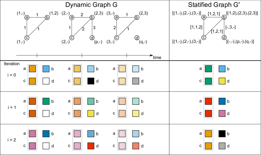
Figure 3: (colored) Illustration of Thm. (4.2.10). In the bottom parts, the dynamic 1-WL test is applied for the dynamic nodes of the dynamic graph $G$ (left side) and the attributed 1-WL test on the static nodes of the statified graph ${G^{\prime}:=\textbf{MakeStatic}(G)}$ (right side). One can see that two dynamic nodes are dynamic 1-WL equivalent if and only if the corresponding static nodes of the statification are attributed 1-WL equivalent. In this example, nodes a and c are dynamic WL equivalent due to the fact that they have the same color in each iteration and at each timestamp on the dynamic graph, as well as in each iteration in the statified graph (emphasized by the gray box).

The next statement Cor. 4.2.11 follows directly from the equivalence between the unfolding trees of the dynamic graphs and their static versions determined in Thm. 4.2.9 and the equivalence between the WL coloring for the same graphs given in Thm. 4.2.10, as well as the equivalence of the attributed WL equivalence and the attributed unfolding tree equivalence formalized in Thm. 4.1.9.

Corollary 4.2.11 (Equivalence of Dynamic WL Equivalence and Dynamic UT Equivalence).

Let $G_{1}=(G^{(1)}_{t})_{t\in I}$ and $G_{2}=(G^{(2)}_{t})_{t\in I}$ be dynamic graphs. Then $G_{1}$ and $G_{2}$ are dynamic WL equivalent if and only if they are dynamic unfolding tree equivalent, i.e.,

$$G_{1}\sim_{DWL}G_{2}\Longleftrightarrow G_{1}\sim_{DUT}G_{2}.$$

5 Approximation Capability of GNN’s

This section brings all the results from Sec. 4.1 and Sec. 4.2 together and formulates a universal approximation theorem for GNNs working on SAUHGs and dynamic graphs and the set of functions that preserve the attributed or dynamic unfolding equivalence, respectively.

5.1 GNN’s for Attributed Static Graphs

Since all the different graph types are lossless transformable into each other [1], it suffices to introduce the GNN architecture of a general model that can handle a SAUHG, as defined in Def. 3.3. For this purpose, the GNN architecture introduced in Def. 3.4 has to be extended to take also edge attributes into account. This can be done including the edge attributes as the edge representation in the first iteration analogously to the processing of the node information in the general GNN framework as follows.

Definition 5.1.1 (SGNN).

For a SAUHG $G=(\mathcal{V},\mathcal{E},\alpha,\omega)$ let $u,v\in\mathcal{V}$ and $e=\{u,v\}$. The SGNN propagation scheme for one iteration $k\in[l]$ is defined as

$$\bm{h}_{v}^{k}=\text{COMBINE}^{(k)}\left(\bm{h}_{v}^{(k-1)},\text{AGGREGATE}^{(k)}\left(\{h_{u}^{k-1}\}_{u\in ne_{v}},\{\omega_{\{u,v\}}\}_{u\in ne_{v}}\right)\right)$$

The output for a node specific learning problem after the last iteration $l$ respectively is given by

$$\bm{z}_{v}=\text{READOUT}\left(\bm{h}_{v}^{l}\right)$$

using a selected AGGREGATION scheme and a suitable READOUT function and the output for a graph specific learning problem is determined by

$$\bm{z}=\text{READOUT}\left(\{\bm{h}_{v}^{l}\mid v\in\mathcal{V}\}\right).$$

Considering the previously defined concepts and statements for SAUHGs in Sec. 4.1, finally the following theorem states the universal approximation capability of the SGNNs on bounded SAUHGs.

Theorem 5.1.2 (Universal Approximation Theorem by SGNN).

Let $\mathcal{G}$ be the domain of bounded SAUHGs with ${r=\max\limits_{G\in\mathcal{G}}\text{diam}(\mathbf{G})}$. For any measurable function $f\in\mathcal{F}(\mathcal{G})$ preserving the attributed unfolding equivalence (cf. Def. 4.1.3), any norm $\|\cdot\|$ on $\mathbb{R}$, any probability measure $P$ on $\mathcal{G}$, for any reals $\epsilon,\lambda$ where $\epsilon>0$, $0<\lambda<1$, there exists a SGNN defined by the continuously differentiable functions $\text{COMBINE}^{(k)}$, $\text{AGGREGATE}^{(k)}$, $\forall k\leq r+1$, and by the function READOUT, with feature dimension $m=1$, i.e, $h_{v}^{k}\in\mathbb{R}$, such that the function $\varphi$ (realized by the GNN) computed after $r+1$ steps for all $\bm{G}\in\mathcal{G}$ satisfies the condition

$$P(\|f(\mathbf{G},v)-\varphi(\mathbf{G},v)\|\leq\varepsilon)\geq 1-\lambda.$$

The corresponding proof can be found in A.7

5.2 GNN’s for Dynamic Graphs

Consistently with the given definition of unfolding trees and WL test for dynamic graphs from Sec. 4.2, the definition of the discrete dynamic graph neural networks (DGNN) provided in [35] can be adopted which uses a GNN to encode each graph snapshot. Here, the model is modified by using the previously defined SGNN 5.1.1 to encode the structural information of each graph snapshot in Def. 5.2.1 and further extended by restricting the function for modeling the temporal behaviour to continuously differentiable recursive functions in Def. 5.2.2.

Definition 5.2.1 (Discrete DGNN).

Given a discrete dynamic graph $G=(G_{t})_{t\in I}$, a discrete DGNN using a function $f$ for temporal modelling can be expressed as:

$$\begin{split}h_{1}(t),\dots,h_{n}(t)&=\text{SGNN}(G_{t})\\ q_{j}(t)&=f(q_{j}(t-1),h_{j}(t))\;\text{for}\;j\in[1,n]\end{split}$$ (2)

where $f:\mathbb{R}^{k}\times\mathbb{R}^{m}\rightarrow\mathbb{R}^{k}$ is a neural architecture for temporal modelling (in the methods surveyed in [35], $f$ is almost always a RNN or a LSTM) and $h_{j}^{t}\in\mathbb{R}^{m}$ is the vector representation of node $j$ at time $t$. Furthermore, $q_{j}^{t}\in\mathbb{R}^{k}$ is a hidden representation of node $j$ produced by $f$. The stacked version of the discrete DGNN is:

$$\begin{split}H(t)&=\text{SGNN}(G_{t})\\ Q(t)&=F(Q(t-1),H(t))\end{split}$$ (3)

where $H(t)\in\mathbb{R}^{n\times m}$, $Q(t)\in\mathbb{R}^{n\times k}$, $F:\mathbb{R}^{n\times k}\times\mathbb{R}^{n\times m}\rightarrow\mathbb{R}^{n\times k}$, being $n$ the number of nodes, $m$ and $k$ the dimensions of the hidden representation of a node produced respectively by the SGNN and by the $f$. Applying $F$ corresponds to component-wise applying $f$ for each node.

Definition 5.2.2 (Message-passing-DGNN).

The Message-passing-DGNN is a particular kind of discrete DGNN where the $f$ and the SGNN of Eq. (2) are respectively any continuously differentiable recursive function and a SGNN that uses the following general updating scheme for the $k-th$ iteration with $k\in[l]$ and for any $t\in I$:

$$\begin{split}{h}_{v}^{k}(t)&=\text{COMBINE}_{t}^{(k)}\left({h}_{v}^{k-1}(t),\text{AGGREGATE}_{t}^{(k)}\{h_{u}^{k-1}(t)\}_{u\in ne_{v}(t)}\right)\end{split}$$

Then $h_{v}(t):=h_{v}^{l}(t)$ is used as input, together with the previous $q_{v}(t-1)$, to the recursive function $f$ Eq. (2).

Finally, the universal approximation of the Message-Passing GNN for dynamic graphs is determined as follows.

Theorem 5.2.3 (Approximation by Message-passing-DGNN).

Let $G=(G_{t})_{t\in I}$ be a discrete dynamic graph in the graph domain $\mathcal{D^{\prime}}$. For each timestamp $t\in I$ we define ${r_{t}=\max\limits_{\mathbf{G_{t}}\in\mathcal{G}}(diam(G_{t}))}$. Let $\text{{dyn}}(t,G,v)\in\mathcal{F}(\mathcal{D^{\prime}})$ be any measurable dynamical system preserving the unfolding equivalence, $\|\cdot\|$ be a norm on $\mathbb{R}$, $P$ be any probability measure on $\mathcal{D^{\prime}}$ and $\epsilon,\lambda$ be any real numbers where $\epsilon>0$, $0<\lambda<1$. Then, there exists a Message-passing-DGNN such that the function $\varphi$ (realized by this model) computed after $r_{t}+1$ steps satisfies the condition

$$P(\|\text{{dyn}}(t,G,v)-\varphi(t,G,v)\|\leq\varepsilon)\geq 1-\lambda\quad\quad\quad\forall t\in I$$

The proof can be found in Apx. A.8.

Theorem 5.2.3 intuitively states that, given a dynamical system dyn, there is a Message Passing DGNN that approximates it. The functions which the Message-Passing DGNN is a composition of (such as the dynamical function $f$, $\text{COMBINE}^{(k)}$, $\text{AGGREGATE}^{(k)}$ etc) are supposed to be continuously differentiable but still generic, while can be generic and completely unconstrained. This situation does not correspond to practical cases, where the Message Passing DGNN adopts particular architectures and those functions are neural networks or, more generally, parametric models — for example made of layers of sum, max, average, etc. Thus, it is of fundamental interest to clarify whether the theorem still holds when the components of the Message-Passing DGNN are parametric models.

Definition 5.2.4.

A class $\cal{Q}$ of discrete DGNN models is said to have universal components if, for any $\epsilon_{1},\epsilon_{2},\epsilon_{3}>0$ and any continuously differentiable target functions $\overline{\text{SGNN}(t)}$, $\overline{f_{0}}$, $\overline{\text{f}}$, there is a discrete DGNN in the class $\cal{Q}$, with functions $\text{SGNN}_{w}(t)$, $f_{0,w}$, $f_{w}$, and parameters $w$ such that, for any input values $\mathbf{G_{t}}$, $\mathbf{q},\mathbf{h}$, it holds

$$\begin{split}\left\|\overline{\text{SGNN}}(\mathbf{G_{t}})-\text{SGNN}_{w}(\mathbf{G_{t}})\right\|_{\infty}&\leq\epsilon_{1},\\ \left\|\overline{f_{0}}(\mathbf{q},\mathbf{h})-f_{0,w}(\mathbf{q},\mathbf{h})\right\|_{\infty}&\leq\epsilon_{2}\;\text{ and }\\ \left\|\overline{f}(\mathbf{q},\mathbf{h})-f_{w}(\mathbf{q},\mathbf{h})\right\|_{\infty}&\leq\epsilon_{3},\;\end{split}$$

where $\|\cdot\|_{\infty}$ is the infinity norm.

Remark 5.2.5.

In Def. 5.2.4 the definition of $\text{SGNN}_{w}(t)$ is well-posed, as we know from [21, Thm. IV.6] that a static parametric $\text{SGNN}(t)_{w}$ exists s.t.

$$\left\|\overline{\text{SGNN}(t)}(\mathbf{G_{t}})-\text{SGNN}(t)_{w}(\mathbf{G_{t}})\right\|_{\infty}\leq\epsilon_{1}$$

The following result shows that Theorem 5.2.3 still holds even for discrete DGNNs with universal components.

Theorem 5.2.6 (Approximation by neural networks).

Assume that the hypotheses of Thm. 5.2.3 are fulfilled and $\cal{Q}$ is a class of GNNs with universal components. Then, there exists a parameter set $w$ and the functions $\text{SGNN}(t)_{w}$, $f_{0,w}$, $f_{w}$, implemented by neural networks in $\cal{Q}$, such that the thesis of Thm. 5.2.3 holds.

The proof can be found in Apx. A.9

5.3 Discussion

The following remarks may further help to understand the results proved in the previous paragraphs:

• Theorem 5.1.2 shows that each message passing GNN considering edge attributes in the aggregation step and whose COMBINE and AGGREGATE functions satisfy specific properties can be a universal approximator for functions on a variety of different domains. Examples are hypergraph domains, multigraph domains, directed graph domains, etc. This result provides an alternative way to design individual GNNs for a specific graph domain. First, each graph in the domain can be transformed into a SAUHG and then a standard message passing GNN (such as OGNN [7], GIN [17] or a GNN characterized by sufficiently "expressive" AGGREGATE and COMBINE functions) can be used.

  as we take into account a discrete recurrent model working on graph snapshots (also known as Stacked DGNN); nevertheless, in [ 15 ] several DGNNs of this kind are listed, such as GCRN-M1 [ 37], RgCNN [ 38], PATCHY-SAN [ 39 ], DyGGNN [40], and others. Still, the approximation capability depends both on the functions AGGREGATE and COMBINE designed for each GNN working on the single snapshot and the implemented recurrent neural network. As an example, the most general model, the original Recurrent Neural Network has been proved to be a universal approximator [41]

• Theorem 5.2.3 doesn’t hold for any Dynamic GNN, as we take into account a discrete recurrent model working on graph snapshots (also known as Stacked DGNN); nevertheless, in[15] several DGNN of this kind are listed, such as GCRN-M1 [36], RgCNN [37], PATCHY-SAN [38], DyGGNN [39], and others. Still, the approximation capability depends both on the functions AGGREGATE and COMBINE designed for each GNN working on the single snapshot and the implemented Recurrent Neural Network. As an example, the most general model, the original RNN, has been proved to be a universal approximator [40].

6 Conclusion

This paper provides two extensions of the 1-WL isomorphism test and the definition of unfolding trees of nodes and graphs. First, we introduced WL test notions to attributed and dynamic graphs, and second, we introduced extended notions for unfolding trees on attributed and dynamic graphs. Further, we proved the existence of a bijection between the dynamic 1-WL equivalence of dynamic graphs and the attributed 1-WL equivalence of their corresponding static versions that are bijective regarding their encoded information. The same result we proved w.r.t. the unfolding tree equivalence. Moreover, we extended the strong connection between unfolding trees and the (dynamic/attributed) 1–WL tests — proving that they give rise to the same equivalence between nodes for the attributed and the dynamic case, respectively. Note that the graph neural networks working on static graphs usually have another architecture than those working on dynamic graphs. Therefore, we have proved that both the different GNN types can approximate any function that preserves the (attributed/dynamic) unfolding equivalence (i.e., the (attributed/dynamic) 1-WL equivalence).

Note that, in this paper, we consider extensions of the usual 1-WL test and the commonly known unfolding trees. One could further investigate extensions, for example, the n-dim attributed/dynamic WL test or other versions of unfolding trees, covering GNN models not considered by the frameworks used in this paper. These extensions might result in a more exemplary classification of the expressive power of different GNN architectures. Moreover, the proposed results mainly focus on the expressive power of GNNs. However, GNNs with the same expressive power may differ for other fundamental properties, e.g., the computational and memory complexity and the generalization capability. Understanding how the architecture of AGGREGATE(k), COMBINE(k), and READOUT impact those properties is of fundamental importance for practical applications of GNNs.

Appendix A Appendix

A.1 Proof of Prop. 4.1.4

A function $f$ belongs to $\mathcal{F}(\mathcal{G})$ if and only if there exists a function $\kappa$ defined on trees such that for any graph $\bm{G}\in\mathcal{G}$ it holds $f(\mathbf{G},v)=\kappa(\mathbf{T}_{v})$, for any node $v\in\bm{G}$.

Proof.

We proof by showing both equivalence directions:

1. If there exists a function $\kappa$ on attributed unfolding trees such that $f(\bm{G},v)=\kappa(\bm{T}_{v})$ for all $v\in G$, then $u\sim_{AUT}v$ for $u,v\in G$ implies $f(\bm{G},u)=\kappa(\bm{T}_{u})=\kappa(\bm{T}_{v})=f(\bm{G},v)$.

2. If $f$ preserves the attributed unfolding equivalence, then a function $\kappa$ on the attributed unfolding tree of an arbitrary node $v$ can be defined as $\kappa(\bm{T}_{v}):=f(\bm{G},v)$. Then, if $\bm{T}_{u}$ and $\bm{T}_{v}$ are two attributed unfolding trees, $\bm{T}_{u}=\bm{T}_{v}$ implies $f(\bm{G},u)=f(\bm{G},v)$ and $\kappa$ is uniquely defined.

∎

A.2 Proof of Lem. 4.1.7

Let $G_{1},G_{2}$ belong to the domain of bounded SAUHGs. Then

$${\forall\,u\in\mathcal{V}_{1},\forall\,v\in\mathcal{V}_{2}:u\sim_{AUT}v\Longleftrightarrow\bm{T}^{r+1}_{u}=\bm{T}^{r+1}_{v}},$$

with $r=\max(\text{diam}(G_{1}),{diam}(G_{2}))$.

Proof.

The proof is completely analogous to the original proof in [23]:

1. By definition, $u\sim_{AUT}v\Longleftrightarrow\bm{T}_{v}=\bm{T}_{u}$, which implies $\bm{T}^{k}_{u}=\bm{T}^{k}_{v}$ for all $k$ and, in particular, also for $k=r+1$.

2. We prove by reductio ad absurdum that $\bm{T}^{k}_{v}=\bm{T}^{k}_{u}\Rightarrow\bm{T}^{k+1}_{v}=\bm{T}^{k+1}_{u}\quad\forall\,k\geq r+1.$ In fact, let us assume that $\exists\;k\geq r+1$ such that $\bm{T}^{k}_{v}=\bm{T}^{k}_{u}$ but $\bm{T}^{k+1}_{v}\neq\bm{T}^{k+1}_{u}$. This means that there would be a node $\mu\in\bm{T}^{k+1}_{v}$ and a node $\nu\in\bm{T}^{k+1}_{u}$ such that $\mu=\nu$ and $\bm{T}^{1}_{\mu}\neq\bm{T}^{1}_{\nu}$, which is impossible, because in $\bm{T}^{k}_{v}$ and $\bm{T}^{k}_{u}$ all nodes have already been explored (since $k\geq r+1$). Moreover, some $i$, with $i\leq r$, exists such that, at depth $i$, an equality holds between subtrees of depth 1 so as $\bm{T}^{1}_{\mu}=\bm{T}^{1}_{\nu}$. Therefore, $\nexists\;k\geq r+1$ such that $\bm{T}^{k}_{v}=\bm{T}^{k}_{u}$ but $\bm{T}^{k+1}_{v}\neq\bm{T}^{k+1}_{u}$ , which proves the theorem.

∎

A.3 Proof of Lem. 4.1.8

Consider ${G^{\prime}=(\mathcal{V}^{\prime},\mathcal{E}^{\prime},\alpha^{\prime},\omega^{\prime})}$ as the SAUHG resulting from a transformation of an arbitrary static graph $G=(\mathcal{V},\mathcal{E},\alpha,\omega)$ with nodes $u,v\in\mathcal{V}$ and corresponding attributes $\alpha_{u},\alpha_{v}$. Then it holds

$$\forall\;d\in\mathbb{N}:\bm{T}^{d}_{u}=\bm{T}^{d}_{v}\Longleftrightarrow c_{u}^{(d)}=c_{v}^{(d)}$$ (4)

Proof.

The proof is carried out by induction on $d$, which represents both the depth of the unfolding trees and the iteration step in the WL colouring.

1. It holds

   $$\quad\bm{T}^{0}_{u}=Tree(\alpha_{u})=Tree(\alpha_{v})=\bm{T}^{0}_{v}\;$$

   $$\Longleftrightarrow\;\alpha_{u}=\alpha_{v}\text{ and }c^{(0)}_{u}=\text{HASH}(\alpha_{u})=\text{HASH}(\alpha_{v})=c^{(0)}_{v}.$$

2. Suppose that Eq. (4) holds for $d-1$, and prove that it holds also for $d$.

   1. By definition, $\bm{T}^{d}_{u}=\bm{T}^{d}_{v}$ is equivalent to

      $$\begin{cases}\bm{T}^{d-1}_{u}=\bm{T}^{d-1}_{v}\quad\text{and}\\ {\small\text{Tree}\bigl{(}\alpha_{u},\Omega_{ne_{u}},\bm{T}^{d-1}_{ne_{u}}\bigr{)}=\text{Tree}\bigl{(}\alpha_{v},\Omega_{ne_{v}},\bm{T}^{d-1}_{ne_{v}}\bigr{)}}.\end{cases}$$ (5)

   2. Applying the induction hypothesis, it holds that

      $$\bm{T}^{d-1}_{u}=\bm{T}^{d-1}_{v}\Longleftrightarrow c^{(d-1)}_{u}=c^{(d-1)}_{v}.$$ (6)

   3. Eq. (5) is equivalent to the following:

      $$\alpha_{u}=\alpha_{v},\quad\Omega_{ne_{u}}=\Omega_{ne_{v}}\quad\textbf{and}\quad\bm{T}^{d-1}_{ne_{u}}=\bm{T}^{d-1}_{ne_{v}}.$$

      Which is equivalent to the existence of an ordering on $ne_{u}$ and $ne_{v}$ s.t.

      $$\begin{cases}\omega_{\{u,ne_{u_{i}}\}}=\omega_{\{v,ne_{v_{i}}\}}\;\forall\;i=1,...,|ne_{u}|\;\text{ and }\\ \bm{T}^{d-1}_{ne_{u_{i}}}=\bm{T}^{d-1}_{ne_{v_{i}}}\;\forall\;i=1,...,|ne_{u}|.\end{cases}$$ (7)

   4. Hence, Eq. (7) hold iff an ordering on $ne_{u}$ and $ne_{v}$ exists s.t.

      $$c^{d-1}_{ne_{u_{i}}}=c^{d-1}_{ne_{v_{i}}}\quad\forall\;i=1,...,|ne_{u}|$$

      $$\text{, \; i.e.,}\quad{|c^{(d-1)}_{m}\mid m\in ne_{u}|}={|c^{(d-1)}_{n}\mid n\in ne_{v}|}.$$

   5. Putting together Eq. (6), (7), and the fact that the HASH function is bijective, we obtain:

      $$\quad\text{HASH}\Bigl{(}\bigl{(}c^{(d-1)}_{u},\Omega_{ne_{u}},{|c^{(d-1)}_{m}\mid m\in ne_{u}|}\bigr{)}\Bigr{)}=$$

      $$=\text{HASH}\Bigl{(}\bigl{(}c^{(d-1)}_{v},\Omega_{ne_{v}},{|c^{(d-1)}_{n}\mid n\in ne_{v}|}\bigr{)}\Bigr{)}$$

      which, by definition, is equivalent to $c^{(d)}_{u}=c^{(d)}_{v}$.

∎

A.4 Proof of Prop. 4.2.6

A dynamic system dyn belongs to $\mathcal{F}(\mathcal{D^{\prime}})$ if and only if there exists a function $\kappa$ defined on trees such that for all $(t,G,v)\in\mathcal{D^{\prime}}$ it holds $\text{{dyn}}(t,G,v)=\kappa\Bigl{(}\bigl{(}\bm{T}_{v}(i)\bigr{)}_{i\in[t]}\Bigr{)}$.

Proof.

We show the proposition by proving both directions of the equivalence relation:

1. If there exists $\kappa$ such that $\text{{dyn}}(t,G,v)=\kappa\Bigl{(}\bigl{(}\bm{T}_{v}(i)\bigr{)}_{i\in[t]}\Bigr{)}$ for all triplets $(t,G,v)\in\mathcal{D^{\prime}}$ then $u\in G^{\prime},v\in G^{\prime\prime}$ with $u\sim_{DUT}v$ implies

   $$\text{{dyn}}(t,G^{\prime},u)=\kappa\Bigl{(}\bigl{(}\bm{T}_{u}(i)\bigr{)}_{i\in[t]}\Bigr{)}=\kappa\Bigl{(}\bigl{(}\bm{T}_{v}(i)\bigr{)}_{i\in[t]}\Bigr{)}=\text{{dyn}}(t,G^{\prime\prime},v).$$

2. On the other hand, if dyn preserves the unfolding equivalence, then we can define $\kappa$ as

   $$\kappa\Bigl{(}\bigl{(}\bm{T}_{v}(i)\bigr{)}_{i\in[t]}\Bigr{)}=\text{{dyn}}(t,G,v).$$

   Note that the above equality is a correct specification for a function. In fact, if

   $$\kappa\Bigl{(}\bigl{(}\bm{T}_{v}(i)\bigr{)}_{i\in[t]}\Bigr{)}=\kappa\Bigl{(}\bigl{(}\bm{T}_{u}(i)\bigr{)}_{i\in[t]}\Bigr{)}$$

   implies $\text{{dyn}}(t,G,u)=\text{{dyn}}(t,G,v)$, then $\kappa$ is uniquely defined.

∎

A.5 Proof of Thm. 4.2.9

Let $G=(G_{t})_{t\in I}$ be a dynamic graph and

$${\textsc{makeStatic}(G)=:G^{\prime}=(\mathcal{V^{\prime}},\mathcal{E^{\prime}},\alpha^{\prime},\omega^{\prime})}$$

the static graph after the transformation. Furthermore, let $\mathcal{V}:=\bigcup_{t\in I}\mathcal{V}_{t}$ be the set of all nodes appearing in the graph sequence of $G$ and $\tilde{\alpha}:\mathcal{V}\times I\rightarrow\mathcal{A}\,\!\perp$ with $\tilde{\alpha}_{v}(t):=(\alpha_{v}(t),\rho)$ be the extended attribute function for all nodes including a flag $\rho\in\{0,1\}$ for the existence of a node at time $t$. Then for all $u,v\in\mathcal{V}$ and $d\in\mathbb{N}$ it holds

$$(\bm{T}_{u}^{d}(t))_{t\in I}=\left(\bm{T}_{v}^{d}(t)\right)_{t\in I}\Longleftrightarrow\bm{T}_{{u}}^{d}=\bm{T}_{{v}}^{d}.$$

Proof.

We prove the statement via induction over $d$.

1. $$\begin{array}[]{cc}&(\bm{T}_{u}^{d}(t))_{t\in I}=(\bm{T}_{v}^{d}(t))_{t\in I}\\ \overset{\text{Def.~{}\ref{def_unfolding_tree_dynamic}}}{\Longleftrightarrow}&\left(Tree(\tilde{\alpha}_{u}(t))\right)_{t\in I}=\left(Tree(\tilde{\alpha}_{v}(t))\right)_{t\in I}\\ \overset{\text{{makeStatic} bij.}}{\Longleftrightarrow}&Tree(\alpha^{\prime}_{u})=Tree(\alpha^{\prime}_{v})\\ \Longleftrightarrow&\bm{T}_{{u}}^{d}=\bm{T}_{{v}}^{d}\end{array}$$

2. Assuming the induction hypothesis (IH) holds for $d-1$, show the hypothesis holds also for $d$.

   $$\begin{array}[]{cc}&(\bm{T}_{u}^{d}(t))_{t\in I}=(\bm{T}_{v}^{d}(t))_{t\in I}\\ \overset{\text{Def.~{}\ref{def_unfolding_tree_dynamic}}}{\Longleftrightarrow}&\left(Tree\left(\tilde{\alpha}_{u}(t),\Omega_{ne_{u}(t)},\bm{T}^{d-1}_{ne_{u}(t)}\right)\right)_{t\in I}=\\ &\left(Tree\left(\tilde{\alpha}_{v}(t),\Omega_{ne_{v}(t)},\bm{T}^{d-1}_{ne_{v}(t)}\right)\right)_{t\in I}\\ \Longleftrightarrow&\tilde{\alpha}_{u}(t)=\tilde{\alpha}_{v}(t)\wedge\Omega_{ne_{u}(t)}=\Omega_{ne_{v}(t)}\wedge\\ &\wedge\;\bm{T}^{d-1}_{ne_{u}(t)}=\bm{T}^{d-1}_{ne_{v}(t)}\forall\;t\in I\\ \overset{\text{IH}}{\Longleftrightarrow}&\alpha^{\prime}_{u}=\alpha^{\prime}_{v}\wedge\Omega_{ne_{u}}=\Omega_{ne_{v}}\wedge\bm{T}^{d-1}_{ne_{u}}=\bm{T}^{d-1}_{ne_{v}}\\ \overset{\text{Def.~{}\ref{def_unfolding_tree_attributed}}}{\Longleftrightarrow}&Tree\bigl{(}\alpha^{\prime}_{u},\Omega_{ne_{u}},\bm{T}^{d-1}_{ne_{u}}\bigr{)}=Tree\bigl{(}\alpha^{\prime}_{v},\Omega_{ne_{v}},\bm{T}^{d-1}_{ne_{v}}\bigr{)}\\ \overset{\text{Def.~{}\ref{def_unfolding_tree_attributed}}}{\Longleftrightarrow}&\bm{T}_{{u}}^{d}=\bm{T}_{{v}}^{d}\end{array}$$

∎

A.6 Proof of Thm. 4.2.10

Let $G=(G_{t})_{t\in I}$ be a dynamic graph and

$${\textsc{makeStatic}(G)=:G^{\prime}=(\mathcal{V^{\prime}},\mathcal{E^{\prime}},\alpha^{\prime},\omega^{\prime})}$$

the SAUHG resulting from a bijective graph type transformation. Furthermore, let $\mathcal{V}:=\bigcup_{t\in I}\mathcal{V}_{t}$ be the set of all nodes appearing in the graph sequence of $G$ and $\tilde{\alpha}:\mathcal{V}\times I\rightarrow\mathcal{A}\,\times\!\perp$ with $\tilde{\alpha}_{v}(t):=(\alpha_{v}(t),\rho)$ be the extended attribute function for all nodes including a flag $\rho\in\{0,1\}$ for the existence of a node at time $t$. Then for an iteration $i$ and $u,v\in\mathcal{V}$ it holds

$$\left(c_{u}^{(i)}(t)\right)_{t\in I}=\left(c_{v}^{(i)}(t)\right)_{t\in I}\Longleftrightarrow c_{{u}}^{(i)}=c_{{v}}^{(i)}.$$

Proof.

We prove the statement by induction over the iteration $i$.

1. $$\begin{array}[]{cc}&\quad\left(c_{u}^{(0)}(t)\right)_{t\in I}=\left(c_{v}^{(0)}(t)\right)_{t\in I}\\ \overset{\text{Def.~{}\ref{def_WL_test_dynamic}}}{\Longleftrightarrow}&\quad\bigl{(}\text{HASH}\left(\tilde{\alpha}_{u}(t)\right)\bigr{)}_{t\in I}=\bigl{(}\text{HASH}\left(\tilde{\alpha}_{v}(t)\right)\bigr{)}_{t\in I}\\ \Longleftrightarrow&\quad\tilde{\alpha}_{u}(t)=\tilde{\alpha}_{v}(t)\quad\forall\;t\in I\\ \overset{\text{by constr.}}{\Longleftrightarrow}&\quad\alpha^{\prime}_{u}=\alpha^{\prime}_{v}\\ \Longleftrightarrow&\quad\text{HASH}\left(\alpha^{\prime}_{u}\right)=\text{HASH}\left(\alpha^{\prime}_{v}\right)\\ \Longleftrightarrow&\quad c_{u}^{(0)}=c_{v}^{(0)}\end{array}$$

2. Assume the induction hypothesis (IH) is true for $i-1$ and show the assumption is also true for $i$.

   $$\begin{array}[]{cc}&\left(c_{u}^{(i)}(t)\right)_{t\in I}=\left(c_{v}^{(i)}(t)\right)_{t\in I}\\ \overset{\text{Def.~{}\ref{def_WL_test_dynamic}}}{\Longleftrightarrow}&\Bigl{(}\text{HASH}\left(c_{u}^{(i-1)}(t),\Omega_{ne_{u}(t)},c_{ne_{u}(t)}^{(i-1)}\right)\Bigr{)}_{t\in I}=\\ &\Bigl{(}\text{HASH}\left(c_{v}^{(i-1)}(t),\Omega_{ne_{v}(t)},c_{ne_{v}(t)}^{(i-1)}\right)\Bigr{)}_{t\in I}\\ \overset{\text{Bij. of HASH}}{\Longleftrightarrow}&c_{u}^{(i-1)}(t)=c_{v}^{(i-1)}(t)\;\wedge\\ &\wedge\;\Omega_{ne_{u}(t)}=\Omega_{ne_{v}(t)}\wedge c_{ne_{u}(t)}^{(i-1)}=c_{ne_{v}(t)}^{(i-1)}\quad\forall\;t\in I\\ \overset{\text{IH}}{\Longleftrightarrow}&c_{u}^{(i-1)}=c_{v}^{(i-1)}\wedge\Omega_{ne_{u}}=\Omega_{ne_{v}}\wedge c_{ne_{u}}^{(i-1)}=c_{ne_{v}}^{(i-1)}\\ \overset{\text{Bij. of HASH}}{\Longleftrightarrow}&\text{HASH}\Bigl{(}\bigl{(}c_{u}^{(i-1)},\Omega_{ne_{u}},c_{ne_{u}}^{(i-1)}\bigr{)}\Bigr{)}\\ &=\text{HASH}\Bigl{(}\bigl{(}c_{v}^{(i-1)},\Omega_{ne_{v}},c_{ne_{v}}^{(i-1)}\bigr{)}\Bigr{)}\\ \overset{\text{Def.~{}\ref{def_WL_test_attributed}}}{\Longleftrightarrow}&c_{{u}}^{(i)}=c_{{v}}^{(i)}\end{array}$$

∎

A.7 Sketch of the proof of Thm. 5.1.2

Since the proof is quite identical to the one in [23], we will only sketch the proof idea below and refer to the original paper for further details. First, we need a preliminary lemma which is an extension of [21, Lem. 1] to the domain of SAUHGs. Intuitively, this lemma suggests that a domain of SAUGH graphs $\mathcal{G}$ with continuous features can be partitioned into small subsets so that the features of the graphs are almost constant in each partition. Moreover, a finite number of partitions is sufficient, in probability, to cover a large part of the domain.

Lemma A.7.1.

For any probability measure $P$ on $\mathcal{D}$, and any reals $\lambda$, $\delta$, where $0<\lambda\leq 1$, $\delta\geq 0$, there exist a real $\bar{b}>0$, which is independent of $\delta$, a set $\bar{\mathcal{D}}\subseteq\mathcal{D}$, and a finite number of partitions $\bar{\mathcal{D}_{1}},\dots,\bar{\mathcal{D}_{l}}$ of $\bar{\mathcal{D}}$, where $\bar{\mathcal{D}}=\mathcal{G}_{i}\times\{v_{i}\}$, with $\mathcal{G}_{i}\subseteq\mathcal{G}$ and $v_{i}\in\mathcal{G}_{i}$, such that:

1. $P(\bar{\mathcal{D}})\geq 1-\lambda$ holds;

2. for each $i$, all the graphs in $\mathcal{G}_{i}$ have the same structure, i.e., they differ only for the values of their labels;

3. for each set $\bar{\mathcal{D}_{i}}$, there exists a hypercube $\mathcal{H}_{i}\in\mathbb{R}^{a}$ such that $\ell_{\mathbf{G}}\in\mathcal{H}_{i}$ holds for any graph $\mathbf{G}\in\mathcal{G}_{i}$, where $\ell_{\mathbf{G}}$ denotes the vector obtained by stacking all the feature vectors of both nodes and edges of $\mathbf{G}$, namely $\ell_{\mathbf{G}}=\ell^{n}_{\mathbf{G}}|\ell^{e}_{\mathbf{G}}$ where $\ell^{n}_{\mathbf{G}}$ is the stacking of all the feature vectors of nodes and $\ell^{e}_{\mathbf{G}}$ is the stacking of all the feature vectors of edges ;

4. for any two different sets $\mathcal{G}_{i}$, $\mathcal{G}_{j}$, $i\neq j$, their graphs have different structures or their hypercubes $\mathcal{H}_{i}$, $\mathcal{H}_{j}$ have a null intersection, i.e. $\mathcal{H}_{i}\bigcap\mathcal{H}_{j}=\emptyset$;

5. for each $i$ and each pair of graphs $\mathbf{G}_{1}$, $\mathbf{G}_{2}\in\mathcal{G}_{i}$, the inequality $\|\ell_{\mathbf{G}_{1}}-\ell_{\mathbf{G}_{2}}\|_{\infty}\leq\delta$ holds;

6. for each graph $\mathbf{G}\in\bar{\mathcal{D}}$, the inequality $\|\ell_{\mathbf{G}}\|_{\infty}\leq\bar{b}$ holds.

Proof.

The proof is quite identical to the one contained in [21]. The only remark needed here is that we can consider the whole stacking of all features from both nodes and edges without loss of generality; indeed, if we were considering separately the node features and the edge features, we would need conditions on the hypercubes s.t.:

$$\begin{split}&\quad\|\ell^{n}_{\mathbf{G}_{1}}-\ell^{n}_{\mathbf{G}_{2}}\|_{\infty}\leq\delta^{n},\;\delta^{n}>0,\\ \text{ and }&\quad\|\ell^{e}_{\mathbf{G}_{1}}-\ell^{e}_{\mathbf{G}_{2}}\|_{\infty}\leq\delta^{e},\;\delta^{e}>0\end{split}$$

then we can stack those feature vectors, as in the statement, s.t. :

$$\begin{split}\|\ell_{\mathbf{G}_{1}}-\ell_{\mathbf{G}_{2}}\|_{\infty}&=\|[\ell^{n}_{\mathbf{G_{1}}}|0]+[0|\ell^{e}_{\mathbf{G_{1}}}]-\bigl{[}[\ell^{n}_{\mathbf{G_{2}}}|0]+[0|\ell^{e}_{\mathbf{G_{2}}}]]\|_{\infty}\\ &\leq\|\ell^{n}_{\mathbf{G_{1}}}-\ell^{n}_{\mathbf{G_{2}}}\|_{\infty}+\|\ell^{e}_{\mathbf{G_{1}}}-\ell^{e}_{\mathbf{G_{2}}}\|_{\infty}\\ &\leq\delta^{n}+\delta^{e}:=\delta\end{split}$$

which allow us to exploit the same proof contained in [21]. ∎

By adopting an argument similar to that in [21], it is proved that Thm. 5.1.2 is equivalent to the following, where the domain contains a finite number of graphs and the features are integers.

Theorem A.7.2.

For any finite set of patterns $\{(\mathbf{G}_{i},v_{i})|\ \mathbf{G}_{i}\in\mathcal{G},v_{i}\in\mathit{N},1\leq i\leq n\}$, with $r=\max\limits_{\mathbf{G}_{i}}\text{diam}(\mathbf{G}_{i})$ and with graphs having integer nodes features, for any function which preserves the attributed unfolding equivalence, and for any real $\varepsilon>0$, there exist continuously differentiable functions $\text{AGGREGATE}^{(k)}$, $\text{COMBINE}^{(k)}$, $\forall\;k\leq r+1$, s.t.

$$\bm{h}_{v}^{k}=\text{COMBINE}^{(k)}\left(\bm{h}_{v}^{(k-1)},\text{AGGREGATE}^{(k)}\left(\{h_{u}^{k-1}\}_{u\in ne_{v}},\{\omega_{\{u,v\}}\}_{u\in ne_{v}}\right)\right)$$

and a function READOUT, with feature dimension $m=1$, i.e, $\mathbf{h}_{v}^{k}\in\mathbb{R}$, so that the function $\varphi$ (realized by the SGNN), computed after $r+1$ steps, satisfies the condition

$$|\tau(\mathbf{G}_{i},v_{i})-\varphi(\mathbf{G}_{i},v_{i})|\leq\varepsilon\quad\text{ for any }i,1\leq i\leq n.$$ (8)

Sketch of the proof.

The idea of the proof is that of designing a GNN that is able to approximate any function $\tau$ that preserves the attributed unfolding equivalence. According to Thm. 4.1.4 there exists a function $\kappa$ s.t. $\tau(\mathbf{G},v)=\kappa(T_{v})$. Therefore, the GNN has to encode the attributed unfolding tree into the node features, i.e., for each node $v$, we want to have $\mathbf{h}_{v}=\triangledown(\mathbf{T}_{v})$, where $\triangledown$ is an encoding function that maps attributed unfolding trees into real numbers. The existence and injectiveness of $\triangledown$ are ensured by construction. More precisely, the encodings are constructed recursively by the $\text{AGGREGATE}^{(k)}$ and the $\text{COMBINE}^{(k)}$ functions using the neighbourhood information, i.e., nodes’ features and edges’ attributes. Therefore, the theorem can be proved provided that there exist appropriate functions $\triangledown$, $\text{AGGREGATE}^{(k)}$, $\text{COMBINE}^{(k)}$ and READOUT. The functions $\text{AGGREGATE}^{(k)}$ and $\text{COMBINE}^{(k)}$ must satisfy

$$\begin{array}[]{lc}\triangledown(\mathbf{T}_{v}^{k})=\bm{h}_{v}^{k}=&\\ ={\scriptsize\text{COMBINE}^{(k)}\left(\bm{h}_{v}^{(k-1)},\text{AGGREGATE}^{(k)}\left(\{h_{u}^{k-1}\}_{u\in ne_{v}},\{\omega_{\{u,v\}}\}_{u\in ne_{v}}\right)\right)}&\\ ={\scriptsize\text{COMBINE}^{(k)}\left(\triangledown(\mathbf{T}_{v}^{k-1}),\text{AGGREGATE}^{(k)}(\{\triangledown(\mathbf{T}^{k-1}_{u}),\;\}_{u\in ne_{v}})\right)}&\\ \end{array}$$

$\forall\;k\leq diam(\mathbf{G})$. In a simple solution, $\text{AGGREGATE}^{(k)}$ decodes the attributed trees of the neighbours $u$ of $v$, $\mathbf{T}^{t-1}_{u}$, and stores them into a data structure to be accessed by $\text{COMBINE}^{(k)}$. ∎

A.8 Proof of Thm. 5.2.3

In order to prove Thm. 5.2.3 we need some preliminary results. Using the same argument used for attributed static graph, we need as a preliminary lemma, the extension of [21, Lem. 1] to the domain of dynamic graphs.

Lemma A.8.1.

For any probability measure $P$ on $\mathcal{D^{\prime}}$, and any reals $\lambda$, $\delta$, where $0<\lambda\leq 1$, $\delta\geq 0$, there exist a real $\bar{b}>0$, which is independent of $\delta$, a set $\bar{\mathcal{D^{\prime}}}\subseteq\mathcal{D^{\prime}}$, and a finite number of partitions $\bar{\mathcal{D^{\prime}}_{1}},\dots,\bar{\mathcal{D^{\prime}}_{l}}$ of $\bar{\mathcal{D^{\prime}}}$, where $\bar{\mathcal{D^{\prime}}}=\mathcal{G}_{i}\times\{v_{i}\}$, with $\mathcal{G}_{i}\subseteq\mathcal{G}$ and $v_{i}\in\mathcal{G}_{i}$, such that:

1. $P(\bar{\mathcal{D^{\prime}}})\geq 1-\lambda$ holds;

2. for each $i$, all the graphs in $\mathcal{G}_{i}$ have the same structure, i.e., they differ only for the values of their labels;

3. for each set $\bar{\mathcal{D^{\prime}}_{i}}$, there exists a hypercube $\mathcal{H}_{i}\in\mathbb{R}^{a}$ such that $\ell_{\mathbf{G}}\in\mathcal{H}_{i}$ holds for any dynamic graph $\mathbf{G}\in\mathcal{G}_{i}$, where $\ell_{\mathbf{G}}$ denotes the vector obtained by stacking all the feature vectors of $\mathbf{G}$ for each timestamp;

4. for any two different sets $\mathcal{G}_{i}$, $\mathcal{G}_{j}$, $i\neq j$, their graphs have different structures or their hypercubes $\mathcal{H}_{i}$, $\mathcal{H}_{j}$ have a null intersection, i.e. $\mathcal{H}_{i}\bigcap\mathcal{H}_{j}=\emptyset$;

5. for each $i$ and each pair of graphs $\mathbf{G}_{1}$, $\mathbf{G}_{2}\in\mathcal{G}_{i}$, the inequality $\|\ell_{\mathbf{G}_{1}}-\ell_{\mathbf{G}_{2}}\|_{\infty}\leq\delta$ holds;

6. for each graph $\mathbf{G}\in\bar{\mathcal{D^{\prime}}}$, the inequality $\|\ell_{\mathbf{G}}\|_{\infty}\leq\bar{b}$ holds.

Proof.

Indeed, taking in account the argument in [1] one can establish a bijection between the domain of dynamic graphs and the domain of SAUHGs; on the latter we can directly apply A.7.1. ∎

Thm. 5.2.3 is equivalent to the following, where the domain contains a finite number of elements in $\mathcal{D^{\prime}}$ and the features are integers.

Theorem A.8.2.

For any finite set of patterns

$$\{(t,G^{(i)},v)|\ (t,G^{(i)},v)\in\mathcal{D^{\prime}},1\leq i\leq n\}$$

with $r_{t}=\max\limits_{G_{t}^{(i)}}\text{diam}(G_{t}^{(i)})$ and with graphs having integer features, for any measurable dynamical system preserving the unfolding equivalence, $\|\cdot\|$ be a norm on $\mathbb{R}$, $P$ be any probability measure on $\mathcal{D^{\prime}}$ and $\epsilon$ be any real number where $\epsilon>0$. Then, there exists a Message-passing-DGNN such that the function $\varphi$ (realized by this model) computed after $r_{t}+1$ steps satisfies the condition

$$||dyn(t,G^{(i)},v)-\varphi(t,G^{(i)},v)||_{m}\leq\varepsilon\quad$$ (9)

$\forall\;i,1\leq i\leq n\;\text{ and }\;\forall\;t\in I.$

The equivalence is formally proved by the following lemma.

Lemma A.8.3.

Thm. 5.2.3 holds if and only if Thm. A.8.2 holds.

Proof.

Thm. 5.2.3 is more general than Thm. A.8.2, which makes this implication straightforward. Suppose instead that Thm. A.8.2 holds and show that this implies Thm. 5.2.3. Let us apply Lem. A.8.1 with values for $P$ and $\lambda$ equal to the corresponding values of Thm. 5.2.3, being $\delta$ any positive real number. It follows that there is a real $\bar{b}$ and a subset $\bar{\mathcal{D^{\prime}}}$ of $\mathcal{D^{\prime}}$ s.t. $P(\bar{\mathcal{D^{\prime}}})>1-\lambda$. Let $\mathcal{M}$ be the subset of $\mathcal{D^{\prime}}$ that contains only the dynamic graphs $\mathbf{G}$ satisfying $\|\ell_{\mathbf{G}}\|_{\infty}\leq\bar{b}$. Note that, since $\bar{b}$ is independent of $\delta$, then $\bar{\mathcal{D^{\prime}}}\subset\mathcal{M}$ for any $\delta$. Since $\tau$ is integrable, there exists a continuous function which approximates $\tau$, in probability, up to any degree of precision. Thus, without loss of generality, we can assume that $\tau$ is equi–continuous on $\mathcal{M}$. By definition of equi–continuity, a real $\bar{\delta}>0$ exists such that

$$|\tau(\mathbf{G}_{1},v)-\tau(\mathbf{G}_{2},v)|\leq\frac{\varepsilon}{2}$$ (10)

holds for any node $v$ and for any pair of dynamic graphs $\mathbf{G}_{1},\mathbf{G}_{2}$ having the same structure and satisfying

$${\|\ell_{\mathbf{G}_{1}}-\ell_{\mathbf{G}_{2}}\|_{\infty}\leq\bar{\delta}}$$

Let us apply Lem. A.8.1 again, where, now, the $\delta$ of the hypothesis is set to $\bar{\delta}$, i.e. $\delta=\bar{\delta}$. From then on, $\bar{\mathcal{D^{\prime}}}=\mathcal{G}_{i}\times\{v_{i}\}$, $1\leq i\leq n$, represents the set obtained by the new application of Lem. A.8.1 and $I_{i}^{\bar{b},\bar{\eta}}$ , $1\leq i\leq 2d$, denotes the corresponding intervals defined in the proof of the same lemma. Let $\theta:\mathbb{R}\rightarrow\mathbb{Z}$ be a function that encodes reals into integers as follows: for any $i$ and any $z\in I_{i}^{\bar{b},\bar{\eta}}$, $\theta(z)=i$. Thus, $\theta$ assigns to all the values of an interval $I_{i}^{\bar{b},\bar{\eta}}$ the index $i$ of the interval itself. Since the intervals do not overlap and are not contiguous, $\theta$ can be continuously extended to the entire $\mathbb{R}$. Moreover, $\theta$ can be extended also to vectors, being $\theta(\mathbf{Z})$ the vector of integers obtained by encoding all the components of $\mathbf{Z}$. Finally, let $\Theta:\mathcal{G}\rightarrow\mathcal{G}$ represent the function that transforms each graph by replacing all the feature labels with their coding, i.e. $\mathbf{L}_{\Theta(\mathbf{G})}=\theta(\mathbf{L}_{\mathbf{G}})$. Let $\bar{\mathbf{G}_{1}},\dots,\bar{\mathbf{G}_{v}}$ be graphs, each one extracted from a different set $\mathcal{G}_{i}$. Note that, according to points 3, 4, 5 of Lem. A.8.1, $\Theta$ produces an encoding of the sets $\mathcal{G}_{i}$. More precisely, for any two graphs $\mathbf{G}_{1}$ and $\mathbf{G}_{2}$ of $\bar{\mathcal{D}}$, we have $\Theta(\mathbf{G}_{1})=\Theta(\mathbf{G}_{2})$ if the graphs belong to the same set, i.e., $\mathbf{G}_{1},\mathbf{G}_{2}\in\mathcal{G}_{i}$, while $\Theta(\mathbf{G}_{1})\neq\Theta(\mathbf{G}_{2})$ otherwise. Thus, we can define a decoding function $\Gamma$ s.t. $\Gamma(\Theta(\bar{\mathbf{G}_{i}}),v_{i})=(\bar{\mathbf{\mathbf{G}_{i}}},v_{i})$, $1\leq i\leq n$.

Consider, now, the problem of approximating $\tau\circ\Gamma$ on the set $(\Theta(\bar{\mathbf{G}_{1}}),v_{1}),\dots,(\Theta(\bar{\mathbf{G}_{n}}),v_{n})$. Thm. A.8.2 can be applied to such a set, because it contains a finite number of graphs with integer labels. Therefore, there exists a Dyn-GNN that implements a function $\bar{\varphi}$ s.t., for each $i$,

$$|\tau(\Gamma(\Theta(\bar{\mathbf{G}_{i}}),v_{i}))-\bar{\varphi}(\Theta(\bar{\mathbf{G}_{i}}),v_{i})|\leq\frac{\varepsilon}{2}$$ (11)

However, this means that there is also another GNN that produces the same result operating on the original graphs $\mathbf{G}_{i}$, namely a GNN for which

$$\varphi(\mathbf{G}_{i},v_{i})=\bar{\varphi}(\Theta(\bar{\mathbf{G}_{i}}),v_{i})\,$$ (12)

holds. Actually, the graphs ${\mathbf{G}_{i}}$ and $\bar{\mathbf{G}_{i}}$ are equal except that the former have the coding of the feature labels attached to the nodes, while the latter contain the whole feature labels. Thus, the GNN that operates on $\bar{\mathbf{G}_{i}}$ is that suggested by Thm. A.8.2, except that $\overline{\text{AGGREGATE}}_{t}^{(0)}$ creates a coding of $\theta(\ell_{v})$ before the rest of the tasks.

Putting together the above equality with Eq. (10) and (11), it immediately follows that, for any $(\mathbf{G},v)\in\bar{\mathcal{D^{\prime}}_{i}}$,

$$\begin{split}|\tau(\mathbf{G},v)-\varphi(\mathbf{G},v)|&=|\tau(\mathbf{G},v)-\tau(\bar{\mathbf{G}_{i}},v)+\tau(\bar{\mathbf{G}_{i}},v)-\varphi(\mathbf{G},v)|\\ &\leq|\tau(\bar{\mathbf{G}_{i}},v)-\varphi(\mathbf{G},v)|+\frac{\varepsilon}{2}\\ &=|\tau(\Gamma(\Theta(\bar{\mathbf{G}_{i}}),v))-\bar{\varphi}(\Theta(\bar{\mathbf{G}_{i}}),v)|+\frac{\varepsilon}{2}\leq\varepsilon\end{split}$$

Thus, the GNN described by Eq. (12) satisfies $|\tau(\mathbf{G},v)-\varphi(\mathbf{G},v)|\leq\varepsilon$ in the restricted domain $\bar{\mathcal{D^{\prime}}}$. Since ${P(\bar{\mathcal{D^{\prime}}})\geq 1-\lambda}$, we have: $P(\|\tau(\mathbf{G},v)-\varphi(\mathbf{G},v)\|\leq\varepsilon)\geq 1-\lambda$ which proves the lemma. ∎

Now, we can proceed to prove Thm. A.8.2.

Proof of Thm. A.8.2.

For the sake of simplicity, the theorem will be proved assuming $m=1$, i.e. $dyn(t,G,v)\in\mathbb{R}$. However, the result can be easily extended to the general case when $dyn(t,G,v)\in\mathbb{R}^{m}$, with $m>1$. According to Thm. 4.2.6, there exists a function $\kappa$ s.t. $dyn(t,G,v)=\kappa((T_{v}(i))_{i\in[t]})$. As a remark, each $T_{v}(i)$ is an attributed unfolding tree. For any timestamp $t$, Thm. 4.1.7 (with $G_{1}=G_{2}$) suggests that an attributed unfolding tree of depth $r+1$, where $r:=\max\limits_{i\in[t]}\text{diam}(\mathbf{G}_{i})$ is enough to store the dynamic graph information, so that $\kappa$ can be designed to satisfy $dyn(t,G,v)=\kappa((T_{v}(i))_{i\in[t]})=\kappa((T_{v}^{r+1}(i))_{i\in[t]})$. Thus, the main idea of the proof consists of designing a Message-passing-DGNN that is able, at each timestamp t, to encode the sequence of attributed unfolding trees $((T_{v}(i))_{i\in[t]}$ into the node features, i.e., for each node $v$, we want to have $q_{v}(t)=\#_{t}((T_{v}(i))_{i\in[t]})$, where $\#_{t}$ is a coding function that maps sequences of $t+1$ attributed trees into real numbers. In order to build a proper encoding which could fit the definition of the Message-passing-DGNN, we need two coding functions: the $\nabla$ function which encodes the attributed unfolding trees, and the family of coding functions $\#_{t}$. In particular, we want the nodes’ features to be defined as composition of coding functions as follows:

$$\begin{split}q_{v}(0)&=f_{0}\left(h_{v}(0)\right)=\#_{0}\left(\nabla^{-1}(h_{v}(0))\right)\\ q_{v}(t)&=\#_{t}\left(\text{APPEND}_{t}\left(\#_{t-1}^{-1}(q_{v}(t-1)),\nabla^{-1}(h_{v}(t))\right)\right)\end{split}$$ (13)

where $f_{0}$ is defined as in 1, the ausiliar function $\text{APPEND}_{t}$ and the $\nabla$, $\#_{t}$ coding functions are defined in the following.

The $\text{APPEND}_{t}$ Function

Definition A.8.4.

Let $\mathcal{T}_{v}^{d}$ be the domain of the attributed unfolding trees with root $v$, up to a certain depth $d$. The function $\text{APPEND}_{t}:\{(T_{v}^{d}(i))_{i\in[t-1]}\}\cup\emptyset\times\mathcal{T}_{v}^{d}\rightarrow\{(T_{v}^{d}(i))_{i\in[t]}\}$ is defined as follows:

$$\text{APPEND}_{0}\bigl{(}\emptyset,\bm{T}_{v}^{d}(0)\bigr{)}:=\bm{T}_{v}^{d}(0)$$

$$\text{APPEND}_{t}\bigl{(}\bigl{(}{\bm{T}_{v}^{d}(0),\ldots,\bm{T}_{v}^{d}(t-1)}\bigr{)},\bm{T}_{v}^{d}(t)\bigr{)}:=$$

$$\bigl{(}\bm{T}_{v}^{d}(0),\ldots,\bm{T}_{v}^{d}(t-1),\bm{T}_{v}^{d}(t)\bigr{)}$$

Intuitively, this function appends the unfolding tree snapshot of the node $v$ at time $t$ to the sequence of the unfolding trees of that node at the previous $t-1$ timestamps.

In the following the coding functions are defined; their existence and injectiveness are provided by construction.

The $\nabla$ Coding Function

Let $\nabla$ be a composition of any two injective functions $\alpha_{\nabla}$ and $\beta_{\nabla}$, $\alpha_{\nabla}\circ\beta_{\nabla}$, with the properties described in the following.

1. $\alpha_{\nabla}$ is an injective function from the domain of static unfolding trees, calculated on the nodes in the graph $G_{t}$, to the Cartesian product $\mathbb{N}\times\mathbb{N}^{P}\times\mathbb{Z}^{\ell_{\mathbf{V}}}=\mathbb{N}^{P+1}\times\mathbb{Z}^{\ell_{\mathbf{V}}}$, where $r_{t}=\max\limits_{G_{t}}\text{diam}(G_{t})$ and $P$ is the maximum number of nodes a tree could have.

   Intuitively, in the Cartesian product, $\mathbb{N}$ represents the tree structure, $\mathbb{N}^{P}$ denotes the node numbering, while, for each node, an integer vector $\in\mathbb{Z}^{\ell_{\mathbf{V}}}$ is used to encode the node features. Notice that $\alpha_{\nabla}$ exists and is injective, since the maximal information contained in an unfolding tree is given by the union of all its node features and all its structural information, which just equals the dimension of the codomain of $\alpha_{\nabla}$.

2. $\beta_{\nabla}$ is an injective function from $\mathbb{N}^{P+1}\times\mathbb{Z}^{\ell_{\mathbf{V}}}$ to $\mathbb{R}$, whose existence is guaranteed by the cardinality theory, since the two sets have the same cardinality.

Since $\alpha_{\nabla_{t}}$ and $\beta_{\nabla_{t}}$ are injective, also the existence and the injectiveness of $\nabla_{t}$ are ensured.

The $\#_{t}$ Coding Family

Similarly as $\nabla$, the $\#_{t}$ functions are composed by two functions $\alpha_{\#_{t}}$ and $\beta_{\#_{t}}$, $\alpha_{\#_{t}}\circ\beta_{\#_{t}}$, with the properties described in the following.

1. $\alpha_{\#_{t}}$ is an injective function from the domain of the dynamic unfolding trees $\mathcal{U}_{t}:=\{({T}^{d}_{v}(i))_{i\in[t]}\}$ to the Cartesian product $\mathbb{N}^{t}\times\mathbb{N}^{tP_{t}}\times\mathbb{Z}^{t\ell_{\mathbf{V}}}=\mathbb{N}^{t(P_{t}+1)}\times\mathbb{Z}^{t\ell_{\mathbf{V}}}$, where $r_{t}=\max\limits_{\mathbf{G}_{t}}\text{diam}(\mathbf{G}_{t})$ and $P_{t}$ is the maximum number of nodes a tree could have (at time t?).

2. $\beta_{\#_{t}}$ is an injective function from $\mathbb{N}^{t(P+1)}\times\mathbb{Z}^{t\ell_{\mathbf{V}}}$ to $\mathbb{R}$, whose existence is guaranteed by the cardinality theory, since the two sets have the same cardinality.

Since $\alpha_{\#_{t}}$ and $\beta_{\#_{t}}$ are injective, also the existence and the injectiveness of $\#_{t}$ are ensured.

The recursive function f and the functions $\text{AGGREGATE}_{t}^{(k)}$ and $\text{COMBINE}_{t}^{(k)}$

The functions $f$ must satisfy

$$\#_{t}\bigl{(}(T_{v}(i))_{i\in[t]}\bigr{)}=\mathbf{q}_{v}(t)=f\bigl{(}\mathbf{q}_{v}(t-1),\mathbf{h}_{v}(t)\bigr{)}$$

where the $\mathbf{h}_{v}(t)$ is the feature of node $v$ at time $t$ extracted from the $t-th$ SGNN, i.e. $\mathbf{h}_{v}(t)=$ SGNN $(G_{t},v)$. In particular, at each iteration $k$, we have

$$\mathbf{h}^{k}_{v}(t)=\text{COMBINE}_{t}^{(k)}\left(\mathbf{h}_{v}^{k-1}(t),\text{AGGREGATE}^{(k)}\left(\{h_{u}^{k-1}(t)\}_{u\in ne_{v}(t)},\{\omega_{\{u,v\}}(t)\}_{u\in ne_{v}(t)}\right)\right)$$

The functions $\text{AGGREGATE}_{t}^{(k)}$ and $\text{COMBINE}_{t}^{(k)}$ – following the proof in [23] – must satisfy

$$\begin{array}[]{lc}\triangledown(\mathbf{T}_{v}^{k}(t))=\mathbf{h}_{v}^{k}(t)=&\\ {\tiny\text{COMBINE}_{t}^{(k)}\left(\mathbf{h}_{v}^{k-1}(t),\text{AGGREGATE}_{t}^{(k)}\left(\{{h}^{k-1}_{u}(t)\;\}_{u\in ne_{v}(t)},\{\omega_{\{u,v\}}(t)\}_{u\in ne_{v}(t)}\right)\right)}&\\ ={\scriptsize\text{COMBINE}_{t}^{(k)}\left(\triangledown(\mathbf{T}_{v}^{k-1}(t)),\text{AGGREGATE}_{t}^{(k)}(\{\triangledown(\mathbf{T}^{k-1}_{u}(t))\;\}_{u\in ne_{v}(t)})\right)}&\end{array}$$

$\forall\;k\leq r_{t}:=diam(G_{t})$ and $\forall\;t\in I$.

For example, the trees can be collected into the coding of a new tree, i.e.,

$$\text{AGGREGATE}_{t}^{(k)}({\triangledown}(\mathbf{T}^{k-1}_{u}(t)),{u\in ne_{v}(t)})={\triangledown}(\cup_{u\in ne_{v}(t)}{\triangledown}^{-1}(\triangledown(\mathbf{T}^{k-1}_{u}(t)))),$$

where $\cup_{u\in ne_{v}(t)}$ denotes an operator that constructs a tree with a root having void features from a set of sub–trees (see Fig. 4). Then, $\text{COMBINE}_{t}^{(k)}$ assigns the correct features to the root by extracting them from $\mathbf{T}^{k-1}_{v}(t)$, i.e.,

$$\text{COMBINE}_{t}^{(k)}({\triangledown}(\mathbf{T}^{k-1}_{v}(t)),b)={\triangledown}(\text{ATTACH}({\triangledown}^{-1}({\triangledown}(\mathbf{T}^{k-1}_{v}(t))),{\triangledown}^{-1}(b))),$$

where ATTACH is an operator that returns a tree constructed by replacing the features of the root in the latter tree with those of the former tree and $b$ is the result of the $\text{AGGREGATE}_{t}^{(k)}$ function.

Figure 4: The ATTACH operator on trees.

Now, notice that, with this definition, $\text{AGGREGATE}_{t}^{(k)}$, $\text{COMBINE}_{t}^{(k)}$, and READOUT may not be differentiable. Nevertheless, Eq. (9) has to be satisfied only for a finite number of graphs, namely $\mathbf{G}_{i}$. Thus, we can specify other functions $\overline{\text{AGGREGATE}_{t}}^{(k)}$, $\overline{\text{COMBINE}_{t}}^{(k)}$, and $\overline{\text{READOUT}}$, which produce exactly the same computations when they are applied on the graphs $\mathbf{G}_{i}$, but that can be extended to the rest of their domain, so that they are continuously differentiable. Obviously, such an extension exists since those functions are only constrained to interpolate a finite number of points.

∎

A.9 Proof of Thm. 5.2.6

Assume that the hypotheses of Thm. 5.2.3 are fulfilled and $\cal{Q}$ is a class of GNNs with universal components. Then, there exists a parameter set $w$ and the functions $\text{SGNN}(t)_{w}$, $f_{0,w}$, $f_{w}$, implemented by neural networks in $\cal{Q}$, such that the thesis of Thm. 5.2.3 holds.

Proof.

The idea of the proof follows from the same reasoning adopted in [21, Cor. 2]. Intuitively, since the discrete DGNN of Thm. 5.2.3 is implemented by continuously differentiable functions, its output depends continuously on the possible changes in the DGNN implementation: small changes in the function implementation cause small changes in the DGNN outputs. Therefore, the functions of the DGNN of Thm. 5.2.3 can be replaced by neural networks, provided that those networks are good approximators.

As in the proof of the dynamic version of the approximation theorem, cf. Thm. 5.2.3, without loss of generality, we will assume that the feature dimension is $n=1$. First of all, note that Thm. 5.2.3 ensures that we can find $\overline{\text{SGNN}(t)}$ (composed by $\overline{\text{COMBINE}^{(k)}(t)}$, $\overline{\text{AGGREGATE}^{(k)}(t)}$ $\forall\;k\leq r_{t}$ and $\overline{\text{READOUT}(t)}$ ) and $\bar{f_{0}}$, $\bar{f}$ so that, for the corresponding function $\bar{\varphi}$ implemented by the DGNN:

$$P(\|\text{{dyn}}(t,G,v)-\bar{\varphi}(t,G,v)\|\leq\frac{\varepsilon}{2})\geq 1-\lambda\quad\quad\quad\forall\;t\in I$$ (14)

Considering that the theorem has to hold only in probability, we can also assume that the domain is bounded, so $\bar{f}(q,h)$ is bounded and has a bounded Jacobian. Let $B$ be a bound on the Jacobian of $\bar{f}(q,h)$ $\forall\;t\in I$ and $\forall\;q$.

Moreover, let $\text{SGNN}_{w}(t)$, $f_{0,w}$, $f_{w}$ be functions implemented by universal neural networks that approximate $\overline{\text{SGNN}(t)}$ and $\bar{f_{0}}$, $\bar{f}$ respectively; let us assume that

$$\|\bar{h}(t)-h_{w}(t)\|=\left\|\overline{\text{SGNN}}(\mathbf{G_{t}})-\text{SGNN}_{w}(\mathbf{G_{t}})\right\|_{\infty}\leq\epsilon_{1},$$

$$\left\|\overline{f_{0}}(\mathbf{q},\mathbf{h})-f_{0,w}(\mathbf{q},\mathbf{h})\right\|_{\infty}\leq\epsilon_{2},$$

$$\text{ and }\left\|\overline{f}(\mathbf{q},\mathbf{h})-f_{w}(\mathbf{q},\mathbf{h})\right\|_{\infty}\leq\epsilon_{3}$$

hold $\forall\;t\in I$ and $\epsilon_{1},\epsilon_{2},\epsilon_{3}>0$.

Let $\bar{F}$, $F_{w}$ be the recursive functions of the DGNNs that are obtained by stacking all the $\bar{f}$ and $f_{w}$ for all the nodes of the input graph ; let $\bar{F}_{0}$, $F_{0,w}$ be the recursive functions of the DGNNs that are obtained by stacking all the $\bar{f}_{0}$ and $f_{0,w}$ for all the nodes of the input graph analogously, let $\bar{H}(t)$ and $H_{w}(t)$ the features produced by $\overline{\text{SGNN}}$, $\text{SGNN}_{w}$ stacked over all the nodes of the input graph. Therefore, we have:

$$\|\bar{H}(t)-H_{w}(t)\|_{\infty}\leq N\epsilon_{1}\;\forall\;t\in I,$$

where $=|G|$ is the number of nodes of the graph input in the SGNN. Additionally, we have that:

$$\begin{array}[]{l}\|\bar{Q}(0)-Q_{w}(0)\|_{\infty}=\|\bar{f}_{0}(\bar{H}(0))-f_{0,w}(H_{w}(0))\|_{\infty}\\ =\|\bar{f}_{0}(\bar{H}(0))-\bar{f}_{0}(H_{w}(0))+\bar{f}_{0}(H_{w}(0))-f_{0,w}(H_{w}(0))\|_{\infty}\\ \leq\|\bar{f}_{0}(\bar{H}(0))-\bar{f}_{0}(H_{w}(0))\|_{\infty}+\|\bar{f}_{0}(H_{w}(0))-f_{0,w}(H_{w}(0))\|_{\infty}\\ \leq N\epsilon_{1}(NB)+N\epsilon_{2}\\ :=\lambda_{0}(\epsilon_{1},\epsilon_{2},\epsilon_{3}).\end{array}$$

With a similar argument,

$$\begin{array}[]{l}\|\bar{Q}(1)-Q_{w}(1)\|_{\infty}=\|\bar{f}(\bar{Q}(0),\bar{H}(1))-f_{w}(Q_{w}(0),H_{w}(1))\|_{\infty}\\ =\|\bar{f}(\bar{Q}(0),\bar{H}(1))-\bar{f}(Q_{w}(0),\bar{H}(1))+\\ \quad+\bar{f}(Q_{w}(0),\bar{H}(1))-\bar{f}(Q_{w}(0),H_{w}(1))+\\ \quad+\bar{f}(Q_{w}(0),H_{w}(1))-f_{w}(Q_{w}(0),H_{w}(1))\|_{\infty}\\ \leq\|\bar{f}(\bar{Q}(0),\bar{H}(1))-\bar{f}(Q_{w}(0),\bar{H}(1))\|_{\infty}+\\ \quad+\|\bar{f}(Q_{w}(0),\bar{H}(1))-\bar{f}(Q_{w}(0),H_{w}(1))\|_{\infty}+\\ \quad+\|\bar{f}(Q_{w}(0),H_{w}(1))-f_{w}(Q_{w}(0),H_{w}(1))\|_{\infty}\\ \leq\lambda_{0}(NB)+N\epsilon_{2}+N\epsilon_{3}\\ :=\lambda_{1}(\epsilon_{1},\epsilon_{2},\epsilon_{3}).\end{array}$$

The above reasoning can then be applied recursively to prove that

$$\|\bar{\varphi}(t,G,v)-\varphi_{w}(t,G,v)\|_{\infty}=\|\bar{Q}(t)-Q_{w}(t)\|_{\infty}=\lambda_{t}(\epsilon_{1},\epsilon_{2},\epsilon_{3}),$$

where $\lambda_{t}(\epsilon_{1},\epsilon_{2},\epsilon_{3})$ could be found as little as possible, according to $\epsilon_{1},\epsilon_{2},\epsilon_{3}$. We choose $\epsilon_{1},\epsilon_{2},\epsilon_{3}$ s.t. $\lambda_{t}\leq\frac{\varepsilon}{2}$. Therefore,

$$P(\|\bar{\varphi}(t,G,v)-\varphi_{w}(t,G,v)\|\leq\frac{\varepsilon}{2})\geq 1-\lambda\quad\quad\quad\forall\;t\in I,$$

which, along with Eq. (14), proves the result. ∎

figs/sbw.jpg Silvia Beddar-Wiesing is a Ph.D. student in Computer Science at the University of Kassel. After her Bachelor in Mathematics with the specialization in Mathematical Optimization in 2017 at the University of Kassel, she changed to Computer Science and absolved her Master Degree with the specialization in Computational Intelligence and Data Analytics in 2020. In her research, she focuses on Machine Learning on structural-dynamic graphs, considering graph preprocessing, representation and embedding techniques. Her further research interests cover topics from Timeseries Analysis, Graph Theory, Machine Learning and Deep Neural Networks.

figs/ale.pdf Giuseppe Alessio D’Inverno is currently a PhD student in Information and Engineering Science at University of Siena. He took a Bachelor Degree in Mathematics in 2018 and a Master Degree cum Laude in Applied Mathematics in 2020. His research interests are mainly focused on mathematical properties of Deep Neural Networks, application of Deep Learning to PDEs, graph theory and geometric modeling. figs/Cate3.pdf Caterina Graziani is currently a Ph.D. student in Information Engineering and Science at the University of Siena. In 2018 she received the Bachelor’s Degree Cum Laude in Mathematics from the University of Siena and two years later she obtained the Master’s Degree Cum Laude in Applied Mathematics at the University of Siena, defending a thesis called “LSTM for the prediction of translation speed based on Ribosome Profiling”. Her research interests are in Graph Theory, Graph Neural Networks and Bioinformatics, with a particular interest on the mathematical foundations of Deep Neural Networks figs/v2.pdf Veronica Lachi is a Ph.D. student in Information and Engineering at the University of Siena. She is graduated in Applied Mathematics with Honors in 2020 and in 2018 she took a bachelor degree in Economics with Honors. Her research interests are mainly focused on Graph Theory, Graph Neural Network, Community Detection in Graphs and Network and mathematical properties of Deep Neural Network. figs/alice.jpeg Alice Moallemy-Oureh is currently a Ph.D. candidate in the University of Kassel, Department of Electrical Engineering and Computer Science. Her topic addresses developing Graph Neural Networks designed to master the handling of attribute-dynamic graphs in continuous time representation. Prior, she graduated with an M.Sc. in Mathematics and its applications to Computer Science from the University of Kassel. Her specialization in Mathematics lies in Algorithmic Commutative Computer Algebra and Geometry. In Computer Science, she focused on Logic and Data Analytics. Further interests cover topics from Graph Theory, Computer Algebra, IT-Security, Geometry, Pattern Recognition, and mathematical properties of Geometric Deep Learning. figs/Fig2.pdf Franco Scarselli received the Laurea degree with honours in Computer Science from the University of Pisa in 1989 and the Ph.D. degree in Computer Science and Automation Engineering from the University of Florence in 1994. After the Ph.D. he has been supported by foundations of private and public companies and by a postdoc of the University of Florence. In 1999, he moved to the University of Siena where he was initially a research associate and, currently, an associate professor at the department of Information Engineering and Mathematics. Franco Scarselli has been involved in several research projects, founded by public institutions and private companies, focused on machine learning, information retrieval and software engineering. Current theoretical research activity is mainly in the field of machine learning with a particular focus on deep learning, graph neural networks, and approximation theory. Research interests include also image understanding, information retrieval and web applications. figs/josephine.jpg Josephine Thomas received her degree in theoretical Physics from TU Berlin and gained her doctorate with a thesis on non-linear dimension reduction applied to a topic of complex network theory from TU Dresden. Currently she is the leader of the junior research group GAIN ’Graphs in Artificial Intelligence and Neural Networks’ at the University of Kassel. Her focus is on Graph Neural Networks for dynamic graphs.

References

- [1] Josephine Maria Thomas and Silvia Beddar-Wiesing and Alice Moallemy-Oureh, Graph Type Expressivity and Transformations, arXiv:2109.10708.
- [2] A. Sperduti, Encoding labeled graphs by labeling raam, Advances in Neural Information Processing Systems 6.
-
[3]
Alessandro Sperduti and Antonina Starita,
Supervised neural networks for the
classification of structures, IEEE Trans. Neural Networks 8 (3) (1997)
714–735.
doi:10.1109/72.572108.
URL https://doi.org/10.1109/72.572108 - [4] C. Goller, A. Kuchler, Learning task-dependent distributed representations by backpropagation through structure, in: Proceedings of International Conference on Neural Networks (ICNN’96), Vol. 1, IEEE, 1996, pp. 347–352.
- [5] A. Micheli, D. Sona, A. Sperduti, Recursive cascade correlation for contextual processing of structured data, in: Proceedings of the 2002 International Joint Conference on Neural Networks. IJCNN’02 (Cat. No. 02CH37290), Vol. 1, IEEE, 2002, pp. 268–273.
- [6] M. Hagenbuchner, A. Sperduti, A. C. Tsoi, A self-organizing map for adaptive processing of structured data, IEEE transactions on Neural Networks 14 (3) (2003) 491–505.
- [7] Franco Scarselli and Marco Gori and Ah Chung Tsoi and Markus Hagenbuchner and Gabriele Monfardini, The Graph Neural Network Model 20 (2009) 61–80. doi:10.1109/TNN.2008.2005605.
- [8] A. Micheli, Neural network for graphs: A contextual constructive approach, IEEE Transactions on Neural Networks 20 (3) (2009) 498–511.
- [9] Y. Li, D. Tarlow, M. Brockschmidt, R. Zemel, Gated graph sequence neural networks, arXiv preprint arXiv:1511.05493.
- [10] J. Bruna, W. Zaremba, A. Szlam, Y. LeCun, Spectral networks and locally connected networks on graphs, in: ICLR 2014, 2014.
- [11] T. N. Kipf, M. Welling, Semi-supervised classification with graph convolutional networks, in: ICLR 2017, 2017.
- [12] W. Hamilton, Z. Ying, J. Leskovec, Inductive representation learning on large graphs, in: Advances in Neural Information Processing Systems, 2017, pp. 1024–1034.
- [13] P. Veličković, et al., Graph attention networks, in: ICLR 2018, 2018.
- [14] P. Battaglia, et al., Relational inductive biases, deep learning, and graph networks, arXiv preprint arXiv:1806.01261.
-
[15]
Seyed Mehran Kazemi and Rishab Goel and Kshitij Jain and Ivan Kobyzev and
Akshay Sethi and Peter Forsyth and Pascal Poupart,
Representation Learning for
Dynamic Graphs: A Survey, J. Mach. Learn. Res. 21 (2020) 70:1–70:73.
URL http://jmlr.org/papers/v21/19-447.html - [16] R. Sato, A Survey on The Expressive Power of Graph Neural Networks, ArXiv abs/2003.04078.
- [17] Xu, Keyulu and Hu, Weihua and Leskovec, Jure and Jegelka, Stefanie, How Powerful are Graph Neural Networks?, arXiv preprint arXiv:1810.00826.
- [18] A. Leman, B. Weisfeiler, A reduction of a graph to a canonical form and an algebra arising during this reduction, Nauchno-Technicheskaya Informatsiya 2 (9) (1968) 12–16.
- [19] Shervashidze, N. and Schweitzer, P. and Van Leeuwen, E. J. and Mehlhorn, K. and Borgwardt, K. M., Weisfeiler-Lehman Graph Kernels, Journal of Machine Learning Research.
-
[20]
Christopher Morris and Martin Ritzert and Matthias Fey and William L. Hamilton
and Jan Eric Lenssen and Gaurav Rattan and Martin Grohe,
Weisfeiler and Leman Go
Neural: Higher-Order Graph Neural Networks, in: The Thirty-Third AAAI
Conference on Artificial Intelligence, AAAI 2019, The Thirty-First
Innovative Applications of Artificial Intelligence Conference, IAAI 2019,
The Ninth AAAI Symposium on Educational Advances in Artificial
Intelligence, EAAI 2019, Honolulu, Hawaii, USA, January 27 - February 1,
2019, AAAI Press, 2019, pp. 4602–4609.
doi:10.1609/aaai.v33i01.33014602.
URL https://doi.org/10.1609/aaai.v33i01.33014602 - [21] Scarselli, Franco and Gori, Marco and Tsoi, Ah Chung and Hagenbuchner, Markus and Monfardini, Gabriele, Computational Capabilities of Graph Neural Networks, IEEE Transactions on Neural Networks 20 (1) (2008) 81–102.
- [22] V. Garg, S. Jegelka, T. Jaakkola, Generalization and representational limits of graph neural networks, in: International Conference on Machine Learning, PMLR, 2020, pp. 3419–3430.
- [23] D’Inverno, Giuseppe Alessio and Bianchini, Monica and Sampoli, Maria Lucia and Scarselli, Franco, A new perspective on the approximation capability of GNNs, arXiv preprint arXiv:2106.08992.
- [24] W. Azizian, M. Lelarge, Expressive power of invariant and equivariant graph neural networks, arXiv preprint arXiv:2006.15646.
- [25] H. Maron, H. Ben-Hamu, N. Shamir, Y. Lipman, Invariant and equivariant graph networks, arXiv preprint arXiv:1812.09902.
- [26] H. Maron, H. Ben-Hamu, H. Serviansky, Y. Lipman, Provably powerful graph networks, Advances in neural information processing systems 32.
- [27] You, Jiaxuan and Gomes-Selman, Jonathan and Ying, Rex and Leskovec, Jure, Identity-Aware Graph Neural Networks, arXiv preprint arXiv:2101.10320.
- [28] Bodnar, Cristian and Frasca, Fabrizio and Wang, Yuguang and Otter, Nina and Montufar, Guido F and Lio, Pietro and Bronstein, Michael, Weisfeiler and Lehman Go Topological: Message Passing Simplicial Networks, in: International Conference on Machine Learning, PMLR, 2021, pp. 1026–1037.
- [29] C. Bodnar, F. Frasca, N. Otter, Y. G. Wang, P. Liò, G. F. Montufar, M. Bronstein, Weisfeiler and Lehman Go Cellular: CW Networks, Advances in Neural Information Processing Systems 34.
- [30] M. Zhang, P. Li, Nested graph neural networks, Advances in Neural Information Processing Systems 34 (2021) 15734–15747.
- [31] R. Abboud, İ. İ. Ceylan, M. Grohe, T. Lukasiewicz, The surprising power of graph neural networks with random node initialization, arXiv preprint arXiv:2010.01179.
- [32] Dasoulas, George and Santos, Ludovic Dos and Scaman, Kevin and Virmaux, Aladin, Coloring Graph Neural Networks for Node Disambiguation, arXiv preprint arXiv:1912.06058.
- [33] Grohe, Martin and Schweitzer, Pascal, The Graph Isomorphism Problem, Communications of the ACM 63 (11) (2020) 128–134.
-
[34]
Michael M. Bronstein and Joan Bruna and Taco Cohen and Petar Velickovic,
Geometric Deep Learning: Grids,
Groups, Graphs, Geodesics, and Gauges, CoRR abs/2104.13478.
arXiv:2104.13478.
URL https://arxiv.org/abs/2104.13478 - [35] J. Skardinga, B. Gabrys, K. Musial, Foundations and Modelling of Dynamic Networks Using Dynamic Graph Neural Networks: A Survey, IEEE Access.
- [36] Y. Seo, M. Defferrard, P. Vandergheynst, X. Bresson, Structured sequence modeling with graph convolutional recurrent networks, in: International conference on neural information processing, Springer, 2018, pp. 362–373.
- [37] A. Narayan, P. H. Roe, Learning graph dynamics using deep neural networks, IFAC-PapersOnLine 51 (2) (2018) 433–438.
- [38] M. Niepert, M. Ahmed, K. Kutzkov, Learning convolutional neural networks for graphs, in: International conference on machine learning, PMLR, 2016, pp. 2014–2023.
- [39] A. Taheri, K. Gimpel, T. Berger-Wolf, Learning to represent the evolution of dynamic graphs with recurrent models, in: Companion proceedings of the 2019 world wide web conference, 2019, pp. 301–307.
- [40] B. Hammer, On the approximation capability of recurrent neural networks, Neurocomputing 31 (1-4) (2000) 107–123.