An Ordinal Latent Variable Model of Conflict Intensity

Abstract

Measuring the intensity of events is crucial for monitoring and tracking armed conflict. Advances in automated event extraction have yielded massive data sets of “who did what to whom” micro-records that enable data-driven approaches to monitoring conflict. The Goldstein scale is a widely-used expert-based measure that scores events on a conflictual–cooperative scale. It is based only on the action category (“what”) and disregards the subject (“who”) and object (“to whom”) of an event, as well as contextual information, like associated casualty count, that should contribute to the perception of an event’s “intensity”. To address these shortcomings, we take a latent variable-based approach to measuring conflict intensity. We introduce a probabilistic generative model that assumes each observed event is associated with a latent intensity class. A novel aspect of this model is that it imposes an ordering on the classes, such that higher-valued classes denote higher levels of intensity. The ordinal nature of the latent variable is induced from naturally ordered aspects of the data (e.g., casualty counts) where higher values naturally indicate higher intensity. We evaluate the proposed model both intrinsically and extrinsically, showing that it obtains good held-out predictive performance.

https://github.com/niklasstoehr/ordinal-conflict-intensity

1 Introduction

On a scale from $-10$ for conflictual to $+10$ for cooperative, which of the following events should be considered more “intense”: “Soldiers injured two civilians” or “Rebels detained fifty soldiers”?

CAMEO code	action name	Goldstein value	avg. # casualties
19	fight	-10.0	9.31
20	mass violence	-10.0	42.20
18	assault	-9.0	11.47
15	force posture	-7.2	0.13
17	coerce	-7.0	1.44
14	protest	-6.5	2.06
13	threaten	-6.0	0.13
10	demand	-5.0	0.01
12	reject	-4.0	0.00
16	reduce relations	-4.0	0.00
9	investigate	-2.0	0.04
11	disapprove	-2.0	0.03
1	public statement	0.0	0.19
4	consult	1.0	0.03
2	appeal	3.0	0.00
5	diplom cooperation	3.5	0.03
3	intent cooperate	4.0	0.05
8	yield	5.0	0.10
6	material cooperation	6.0	0.01
7	provide aid	7.0	0.00

Table 1: The The Goldstein scale is an expert-based intensity ranking of the $20$ CAMEO action categories ranging between $-10.0$ (conflictual) to $+10.0$ (cooperative). The scale disregards casualty counts that are typically considered in conflict assessment. Here, we display casualty counts as reported in the NAVCO dataset.

Measuring the intensity of events is crucial for monitoring and tracking armed conflict. Advances in the automated collection and coding of events have produced massive and systematized data sets of micro-records that enable data-driven approaches to monitoring conflict. While the “intensity” of a given event has traditionally been assessed by human expert raters, the tremendous quantity of events collected every day makes case-by-case analysis unmanageable. As a consequence, there is a strong demand for automated and model-based methods to aggregate events into meaningful “conflict intensity” measures.

One of the most frequently used measures is the Goldstein scale (Goldstein, 1992). Major event datasets like IDEA (Bond et al., 2003), KEDS (Schrodt, 2008), GDELT (Leetaru and Schrodt, 2013), ICEWS (Boschee et al., 2015), Phoenix (Beieler, 2016) and NAVCO (Lewis et al., 2016) all rely on it. The Goldstein scale assigns intensity scores between $-10.0$ and $+10$ on a conflictual–cooperative scale to the action categories defined by the Conflict and Mediation Event Observations (CAMEO) event coding scheme (Schrodt, 2012). CAMEO specifies $204$ low-level event types which are summarized into $20$ high-level action categories. The Goldstein scale ranks “use unconventional mass violence” and “fight” as the most conflictual of the 20 high-level action categories ($-10.0$) and “provide aid” ($+7.0$) as the most cooperative; see Tab. 1.

Despite its usage, the Goldstein scale has many well-known shortcomings (King and Lowe, 2003; Schrodt, 2019). In particular, it applies only to action categories, and does not account for any contextual information of a given event, like which actors are involved, or how many fatalities resulted, among other bits of context that should contribute to the perception of an event’s “intensity”.

This paper takes a latent-variable based approach to measuring conflict intensity. We introduce a probabilistic generative model that assumes each observed event $n$ is associated with a latent intensity class $z_{n}$. A novel aspect of this model is that it imposes an ordering on the classes, such that higher values of $z_{n}$ denote higher levels of intensity. The ordinal nature of $z_{n}$ is induced from naturally ordered aspects of the data (e.g., casualty counts) where higher values naturally indicate higher intensity. The model effectively learns to interpolate the ordered (i.e., cardinal or ordinal) elements of the data while inferring correlation structure with the non-ordered (e.g., categorical) elements of the data (e.g., actor types).

We start with a discussion of the Goldstein scale and introduce a political event dataset annotated with Goldstein values in § 2 and § 3. Then, we propose our model with an ordinal latent variable in § 4. We evaluate the performance of the model intrinsically (§ 5) and extrinsically (§ 6) and find that it improves over measures based on the original Goldstein scale or heuristics based on the raw data.

2 Limitations of the Goldstein Scale

The Goldstein scale is a widely-used measure of the conflictual versus cooperative nature of interactions between countries (Goldstein, 1992). The scale was created by a panel of international relations experts who ranked descriptions of interactions. It was initially created to score action categories in the WEIS event ontology (McClelland, 1984) and was later adapted to CAMEO (Schrodt, 2012).

The Goldstein scale applies only to the action category of an event (e.g., “fight” or “trade”). Thus, two different “fight” events, which might involve two different pairs of actors, occur at different times, or differ dramatically with respect to the number of associated fatalities, will still be assigned the same Goldstein value. The Goldstein scale is thus a poor measure of a conflict’s perceived “intensity”, as it ignores much of the information that contributes to that perception. Recent work in conflict studies, for instance, operationalizes “intensity” primarily using casualty counts (Chaudoin et al., 2017; Zhong et al., 2023), which the Goldstein scale ignores entirely.

In Tab. 1, we show the empirical distribution of assigned Goldstein values alongside the empirical distribution of casualty counts in a dataset of conflict events. The Goldstein scale is very coarse-grained; while it ostensibly ranges between $-10.0$ and $+10.0$, only a small number of discrete values ever occur, with many action categories assigned the same value. For the purpose of measuring conflict intensity, a finer-grained and more contextual scale is desirable.

3 Conflict Event Data

This paper considers the publicly available Nonviolent and Violent Campaigns and Outcomes (NAVCO) data collection (Chenoweth et al., 2018), specifically, the latest release NAVCO 3.0 from November 2019 which comprises $N=$112089$$ events between December 1990 and December 2012. An exemplary event description is “On 19 May 2012, soldiers injured two civilians in Afghanistan”. Each part of this description has been parsed by human coders into standardized, structural features. We color-code the features that correspond to the semantic roles subject, predicate, quantifier, object, which are the focus of our modeling approach. Each data point $n$ thus consists of a four-element tuple $\{{\color[rgb]{0.046875,0.0703125,0.76171875}s_{n}},{\color[rgb]{0.5234375,0.046875,0.76171875}p_{n}},{\color[rgb]{0.76171875,0.046875,0.5234375}q_{n}},{\color[rgb]{0.046875,0.703125,0.76171875}o_{n}}\}$. We note that events are further coded for their location (in this case, Afghanistan) and time (19 May 2012), among other bits of contextual information. Let us discuss each feature in more detail:

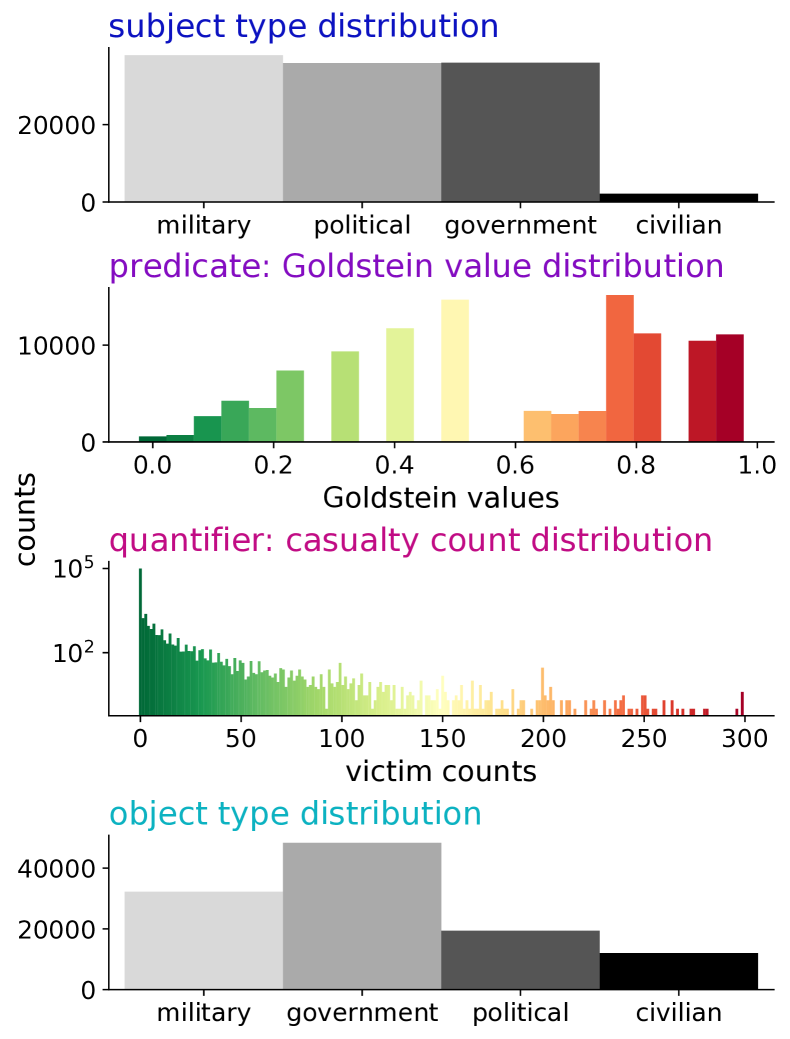
Figure 1: Data distributions of NAVCO 3.0 dataset (Chenoweth et al., 2018). Goldstein values and casualty counts have intrinsic intensity orderings. Goldstein values are reversed and transformed, so that $1.0$ represents the most conflictual. We model the subject ${\color[rgb]{0.046875,0.0703125,0.76171875}s_{n}}$ as Categorical, the predicate ${\color[rgb]{0.5234375,0.046875,0.76171875}p_{n}}$ as Beta, the quantifier ${\color[rgb]{0.76171875,0.046875,0.5234375}q_{n}}$ as Zero-inflated Geometric and the object ${\color[rgb]{0.046875,0.703125,0.76171875}o_{n}}$ as Categorical. 

Subject ${\color[rgb]{0.046875,0.0703125,0.76171875}s_{n}}$.

NAVCO contains columns termed “actor3”, “actor6” and “actor9” which code for the subject (or agent) of a given action. The actor types are defined by the CAMEO actor codebook. We first merge the higher-level categories “actor3” and “actor6”, resulting in $33$ different actor types, and then map all actor types into one of $S=4$ classes: ${\color[rgb]{0.046875,0.0703125,0.76171875}s_{n}}\in\{\text{civilian},\text{military},\text{governmental},\text{political}\}$. We present our $4$-class actor type mapping in Tab. 3 of the appendix.

Predicate ${\color[rgb]{0.5234375,0.046875,0.76171875}p_{n}}$ (Goldstein values).

NAVCO codes each event description into one of the 20 CAMEO action categories in the column “verb10”, which is by extension associated with a Goldstein value ${\color[rgb]{0.5234375,0.046875,0.76171875}p_{n}}$. Throughout, we refer to the Goldstein value ${\color[rgb]{0.5234375,0.046875,0.76171875}p_{n}}$ as an action’s “predicate”, since there is a one-to-one mapping between action categories and Goldstein values. We scale Goldstein values ${\color[rgb]{0.5234375,0.046875,0.76171875}p_{n}}$ to a $[0,1]$ range and invert them (i.e., ${\color[rgb]{0.5234375,0.046875,0.76171875}p_{n}}\leftarrow 1-{\color[rgb]{0.5234375,0.046875,0.76171875}p_{n}}$) so that higher values close to $1$ represent more conflictual action categories.

Quantifier ${\color[rgb]{0.76171875,0.046875,0.5234375}q_{n}}$ (casualty counts).

Each event description is annotated with human-verified fatality and wounded counts. We add the two and refer to the resulting value ${\color[rgb]{0.76171875,0.046875,0.5234375}q_{n}}\in\mathbb{N}_{0}^{+}$ as an event’s “quantifier” or its “casualty count”. In Tab. 1, we give the average number of casualties associated with each action alongside its Goldstein value—as intuition might suggest, actions that Goldstein scores as more conflictual (e.g., “fight” ($-10.0$)) coincide with more casualties on average.

Object ${\color[rgb]{0.046875,0.703125,0.76171875}o_{n}}$.

Similar to its subject, NAVCO codes for the direct object or “target” of a conflict action using the CAMEO coding scheme; these codes are found in the columns “target3” and “target6”. We map those into the $O=$ $4$ classes so that ${\color[rgb]{0.046875,0.703125,0.76171875}o_{n}}\in\{\text{civilian},\text{military},\text{governmental},\text{political}\}$.

Contextual information: location and time.

Finally, each event is further annotated with a timestamp and location, which we use to design extrinsic evaluation tasks in § 6.

4 Ordinal Latent Variable Model

We operationalize conflict intensity as a latent variable that expresses the association between the observed variables subject (${\color[rgb]{0.046875,0.0703125,0.76171875}s_{n}}$), predicate (${\color[rgb]{0.5234375,0.046875,0.76171875}p_{n}}$), quantifier (${\color[rgb]{0.76171875,0.046875,0.5234375}q_{n}}$) and object (${\color[rgb]{0.046875,0.703125,0.76171875}o_{n}}$). Each data point is a tuple $\{{\color[rgb]{0.046875,0.0703125,0.76171875}s_{n}},{\color[rgb]{0.5234375,0.046875,0.76171875}p_{n}},{\color[rgb]{0.76171875,0.046875,0.5234375}q_{n}},{\color[rgb]{0.046875,0.703125,0.76171875}o_{n}}\}$ representing an event. Our Bayesian latent variable model is depicted in Fig. 2. We assume the following generative story. For each event $n$, we assume that its event intensity class $z_{n}\in\{1,\ldots,C\}$ is a Categorical random variable

$$z_{n} \sim\mathrm{Categorical}({\boldsymbol{\pi}}^{(z)})$$ (1)

where ${\boldsymbol{\pi}}^{(z)}$ is a $C$-dimensional discrete distribution over latent intensity classes. We place a Dirichlet prior over ${\boldsymbol{\pi}}^{(z)}$

$${\boldsymbol{\pi}}^{(z)} \sim\mathrm{Dirichlet}(\boldsymbol{\alpha}^{(z)})$$ (2)

with concentration parameter $\boldsymbol{\alpha}^{(z)}\in\mathbb{R}_{+}^{C}$. Conditioned on $z_{n}$, we assume each of the observed sites per event tuple ${\color[rgb]{0.046875,0.0703125,0.76171875}s_{n}},{\color[rgb]{0.5234375,0.046875,0.76171875}p_{n}},{\color[rgb]{0.76171875,0.046875,0.5234375}q_{n}}$ and ${\color[rgb]{0.046875,0.703125,0.76171875}o_{n}}$ are then drawn as

$${\color[rgb]{0.046875,0.0703125,0.76171875}s_{n}}\mid z_{n} \sim\mathrm{Categorical}({\color[rgb]{0.046875,0.0703125,0.76171875}{\boldsymbol{\pi}}^{(s)}_{z_{n}}})$$ (3)

$${\color[rgb]{0.5234375,0.046875,0.76171875}p_{n}}\mid z_{n} \sim\mathrm{Beta}({\color[rgb]{0.5234375,0.046875,0.76171875}\omega^{(p)}_{z_{n}}},{\color[rgb]{0.5234375,0.046875,0.76171875}\kappa^{(p)}_{z_{n}}})$$ (4)

$${\color[rgb]{0.76171875,0.046875,0.5234375}q_{n}}\mid z_{n} \sim\mathrm{Zero\text{-}infl.\text{ }Geom.}({\color[rgb]{0.76171875,0.046875,0.5234375}\delta^{(q)}_{z_{n}}},{\color[rgb]{0.76171875,0.046875,0.5234375}b^{(q)}_{z_{n}}})$$ (5)

$${\color[rgb]{0.046875,0.703125,0.76171875}o_{n}}\mid z_{n} \sim\mathrm{Categorical}({\color[rgb]{0.046875,0.703125,0.76171875}{\boldsymbol{\pi}}^{(o)}_{z_{n}}})$$ (6)

Here ${\color[rgb]{0.046875,0.0703125,0.76171875}{\boldsymbol{\pi}}^{(s)}_{z_{n}}}$ and ${\color[rgb]{0.046875,0.703125,0.76171875}{\boldsymbol{\pi}}^{(o)}_{z_{n}}}$ are the discrete distributions for class $z_{n}$ over $S$ subject and $O$ object types, respectively. They are given as row vectors in the matrices ${\color[rgb]{0.046875,0.0703125,0.76171875}\boldsymbol{\Pi^{(s)}}}\in(0,1)^{C\times S}$ and ${\color[rgb]{0.046875,0.703125,0.76171875}\boldsymbol{\Pi^{(o)}}}\in(0,1)^{C\times O}$ that $z_{n}$ indexes into. We place a simple symmetric Dirichlet prior over all rows—e.g., ${\color[rgb]{0.046875,0.0703125,0.76171875}{\boldsymbol{\pi}}^{(s)}_{c}}\sim\mathrm{Dirichlet}(\mathbf{1}_{S})$ for $c\in\{1,\dots,C\}$. The scalar parameters ${\color[rgb]{0.5234375,0.046875,0.76171875}\omega^{(p)}_{z_{n}}},{\color[rgb]{0.5234375,0.046875,0.76171875}\kappa^{(p)}_{z_{n}}},{\color[rgb]{0.76171875,0.046875,0.5234375}\delta^{(q)}_{z_{n}}},{\color[rgb]{0.76171875,0.046875,0.5234375}b^{(q)}_{z_{n}}}$ are similarly selected by $z_{n}$ from $C$-dimensional vectors ${\color[rgb]{0.5234375,0.046875,0.76171875}{\boldsymbol{\omega}}^{(p)}},{\color[rgb]{0.5234375,0.046875,0.76171875}{\boldsymbol{\kappa}}^{(p)}},{\color[rgb]{0.76171875,0.046875,0.5234375}{\boldsymbol{\delta}}^{(q)}},{\color[rgb]{0.76171875,0.046875,0.5234375}{\mathbf{b}}^{(q)}}$ as discussed below.

Figure 2: The proposed latent variable model of conflict intensity. The observed sites of an event tuple $\{{\color[rgb]{0.046875,0.0703125,0.76171875}s_{n}},{\color[rgb]{0.5234375,0.046875,0.76171875}p_{n}},{\color[rgb]{0.76171875,0.046875,0.5234375}q_{n}},{\color[rgb]{0.046875,0.703125,0.76171875}o_{n}}\}$ describe the subject type, Goldstein value, casualty counts, object type in an event description such as “ soldiers injured two civilians”. The parameters ${\color[rgb]{0.5234375,0.046875,0.76171875}{\boldsymbol{\omega}}^{(p)}}$, ${\color[rgb]{0.76171875,0.046875,0.5234375}{\boldsymbol{\delta}}^{(q)}}$ and ${\color[rgb]{0.76171875,0.046875,0.5234375}{\mathbf{b}}^{(q)}}$ are ordinally transformed vectors, as indicated by double-border nodes ( ) which leads the latent $z_{n}$ to represent ordinal intensity classes.

4.1 Ordinal Latent Variable

We want the latent variable $z_{n}$ to be ordinal, such that higher-valued classes correspond to higher intensity levels. However, in the model thus described, $z_{n}$ is a Categorical random variable whose classes are not inherently ordered. So how does this model encode an ordinal $z_{n}$? Unlike the subject ${\color[rgb]{0.046875,0.0703125,0.76171875}s_{n}}$ and object ${\color[rgb]{0.046875,0.703125,0.76171875}o_{n}}$, which are categorical, the Goldstein value ${\color[rgb]{0.5234375,0.046875,0.76171875}p_{n}}$ and casualty count ${\color[rgb]{0.76171875,0.046875,0.5234375}q_{n}}$ are cardinal quantities whose magnitudes naturally indicate the “intensity” of a given event. To capture this intuition, we first assume that ${\color[rgb]{0.5234375,0.046875,0.76171875}p_{n}}$ and ${\color[rgb]{0.76171875,0.046875,0.5234375}q_{n}}$ are drawn from Beta (eq. 4) and Zero-inflated Geometric distributions (eq. 5), respectively, whose parameters are indexed by $z_{n}$. We then impose an ordering on the parameters, such that higher classes (e.g., $z_{n}=c$) correspond to higher-valued parameters (e.g., ${\color[rgb]{0.5234375,0.046875,0.76171875}\omega^{(p)}_{c}}>{\color[rgb]{0.5234375,0.046875,0.76171875}\omega^{(p)}_{c-1}}$) which in turn encourage larger values of the observed cardinal quantities (e.g., ${\color[rgb]{0.5234375,0.046875,0.76171875}p_{n}}$). 

Ordered Normal

To flexibly impose ordering on vectors of parameters, we first define the Ordered Normal prior (Stoehr et al., 2023a). An ordered vector ${\boldsymbol{\lambda}}=(\lambda_{1},\ldots,\lambda_{C})$, where $\lambda_{c}>\lambda_{c-1}$, is a $C$-dimensional Ordered Normal random variable ${\boldsymbol{\lambda}}\sim\mathrm{OrderedNormal}_{C}(\mu,\sigma)$ if it is sampled according to the following generative process:

$$x_{c}\stackrel{{\scriptstyle\textrm{iid}}}{{\sim}}\mathrm{Normal}(\mu,\sigma)\quad\text{ for }c\in\{1,\,\dots\,,C\}$$

$$(\lambda_{1},\dots,\lambda_{C})\leftarrow\mathrm{Ord}(\{x_{1},\dots,x_{C}\})$$ (7)

where $\mathrm{Ord}(\cdot)$ takes in an unordered set of numbers $\{x_{1},\dots,x_{C}\}$, and transforms it into a vector whose components are in strictly increasing order,

$$\lambda_{c}\leftarrow\begin{cases}x_{1}&\text{if }c=1\\ x_{1}+\sum_{i=2}^{c}\exp({x_{i}})&\text{if }c>1\end{cases}$$ (8)

This transformation is invertible and differentiable and thus does not obstruct gradient-based inference of model parameters (App. B).

Ordered Beta.

We model Goldstein values ${\color[rgb]{0.5234375,0.046875,0.76171875}p_{n}}$ as Beta random variables. For intensity class $z_{n}=c$, we assume ${\color[rgb]{0.5234375,0.046875,0.76171875}p_{n}}\sim\mathrm{Beta}({\color[rgb]{0.5234375,0.046875,0.76171875}\omega^{(p)}_{c}},{\color[rgb]{0.5234375,0.046875,0.76171875}\kappa^{(p)}_{c}})$, where ${\color[rgb]{0.5234375,0.046875,0.76171875}\omega^{(p)}_{c}}\in(0,1)$ is the mode and ${\color[rgb]{0.5234375,0.046875,0.76171875}\kappa^{(p)}_{c}}>0$ is the concentration parameter. We impose an ordering on the modes by positing a transformed OrderedNormal prior:

$$S^{-1}({\color[rgb]{0.5234375,0.046875,0.76171875}{\boldsymbol{\omega}}^{(p)}}) \sim\mathrm{OrderedNormal}_{C}(\mu,\sigma)$$ (9)

where ${\color[rgb]{0.5234375,0.046875,0.76171875}{\boldsymbol{\omega}}^{(p)}}=({\color[rgb]{0.5234375,0.046875,0.76171875}\omega^{(p)}_{1}},\ldots,{\color[rgb]{0.5234375,0.046875,0.76171875}\omega^{(p)}_{C}})$ is the $C$-dimensional ordered vector of modes and $S^{-1}(\cdot)$ is the element-wise inverse sigmoid function. To ensure that each class-conditional Beta distribution is unimodal around its mode ${\color[rgb]{0.5234375,0.046875,0.76171875}\omega^{(p)}_{c}}$, we then mandate that the concentration parameter ${\color[rgb]{0.5234375,0.046875,0.76171875}\kappa^{(p)}_{c}}$ is greater than 2 by imposing a shifted Gamma prior.

$$({\color[rgb]{0.5234375,0.046875,0.76171875}\kappa^{(p)}_{c}}-2) \stackrel{{\scriptstyle\textrm{iid.}}}{{\sim}}\mathrm{Gamma}(k,\eta)$$ (10)

where $k$ and $\eta$ are the shape and rate parameters. We note that while the elements of ${\color[rgb]{0.5234375,0.046875,0.76171875}{\boldsymbol{\omega}}^{(p)}}$ are ordered, those of ${\color[rgb]{0.5234375,0.046875,0.76171875}{\boldsymbol{\kappa}}^{(p)}}$ are not.

Ordered Zero-inflated Geometric.

We model the casualty counts ${\color[rgb]{0.76171875,0.046875,0.5234375}q_{n}}$ as Zero-inflated Geometric random variables. For intensity class $z_{n}=c$, we assume ${\color[rgb]{0.76171875,0.046875,0.5234375}q_{n}}\sim\mathrm{Zero\text{-}infl.\text{ }Geom.}({\color[rgb]{0.76171875,0.046875,0.5234375}\delta^{(q)}_{c}},{\color[rgb]{0.76171875,0.046875,0.5234375}b^{(q)}_{c}})$ where ${\color[rgb]{0.76171875,0.046875,0.5234375}\delta^{(q)}_{c}}\in(0,1)$ is the “gate” parameter—i.e., the inflated probability of sampling a zero—and ${\color[rgb]{0.76171875,0.046875,0.5234375}b^{(q)}_{c}}\in(0,1)$ is the success probability parameter under the standard Geometric distribution. We impose an ordering on both $C$-dimensional vectors of parameters ${\color[rgb]{0.76171875,0.046875,0.5234375}{\boldsymbol{\delta}}^{(q)}}$ and ${\color[rgb]{0.76171875,0.046875,0.5234375}{\mathbf{b}}^{(q)}}$ using the same transformed Ordered Normal prior as in the previous subsection:

$$S^{-1}({\color[rgb]{0.76171875,0.046875,0.5234375}{\boldsymbol{\delta}}^{(q)}}) \sim\mathrm{OrderedNormal}_{C}(\mu,\sigma)$$ (11)

$$S^{-1}({\color[rgb]{0.76171875,0.046875,0.5234375}{\mathbf{b}}^{(q)}}) \sim\mathrm{OrderedNormal}_{C}(\mu,\sigma)$$ (12)

Importantly though, we reverse the ordering of ${\boldsymbol{\lambda}}$ such that for all $c\in\{1,\ldots,C\}:\lambda_{c}<\lambda_{c-1}$. The reason is that higher ${\color[rgb]{0.76171875,0.046875,0.5234375}\delta^{(q)}_{c}}$ and ${\color[rgb]{0.76171875,0.046875,0.5234375}b^{(q)}_{c}}$ correspond, on average, to lower values sampled from the Zero-inflated Geometric and thus lower casualty counts and lower event intensity.

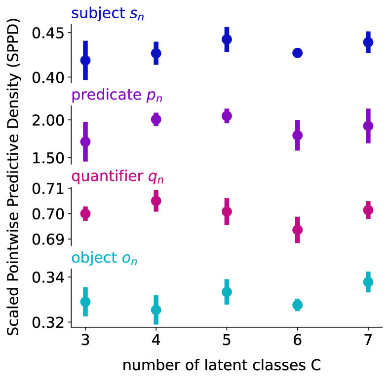
Figure 3: Determining the optimal number of latent classes $C$. The values show the mean and standard deviation of the scaled pointwise predictive density (SPPD) on the held-out dataset over $5$ random seeds. A model with $C=5$ latent classes fits the data best overall.

4.2 Posterior Inference

We implement the model using the probabilistic programming framework Pyro (Bingham et al., 2018). Pyro provides an OrderedTransform function that implements eq. 8. We approximate the posterior distribution of our model’s parameters using the No-U-Turn Sampler (NUTS; Homan and Gelman, 2014), a variant of Hamiltonian Monte Carlo. NUTS is gradient-based and requires the parameters to be continuous. However, we explicitly model our latent variable $z_{n}$ to be ordinal. To solve this problem, Pyro provides parallel_enumeration which marginalizes out discrete variables numerically during inference. We refer to all continuous parameters of our model as $\theta=\{{\boldsymbol{\pi}}^{(z)},{\color[rgb]{0.046875,0.0703125,0.76171875}\boldsymbol{\Pi^{(s)}}},{\color[rgb]{0.5234375,0.046875,0.76171875}{\boldsymbol{\omega}}^{(p)}},{\color[rgb]{0.5234375,0.046875,0.76171875}{\boldsymbol{\kappa}}^{(p)}},{\color[rgb]{0.76171875,0.046875,0.5234375}{\boldsymbol{\delta}}^{(q)}},{\color[rgb]{0.76171875,0.046875,0.5234375}{\mathbf{b}}^{(q)}},{\color[rgb]{0.046875,0.703125,0.76171875}\boldsymbol{\Pi^{(o)}}}\}$ and to the full dataset of event tuples as $X$. NUTS produces samples of $\theta$ from the posterior $\theta^{(t)}\sim p(\theta\mid X)$. We can further sample the ordinal latent $z_{n}^{(t)}\sim p(z_{n}\mid\theta^{(t)},X)$ using Pyro’s infer_discrete. Based on the samples $\{z_{n}^{(t)}\}_{t=1}^{T}$ per event $n$, we can then compute a point estimate of the event’s ordinal intensity either by taking the mean $\bar{z}_{n}=\frac{1}{T}\sum_{t=1}^{T}z_{n}^{(t)}$ or the mode (i.e., the most frequently sampled class) $\dot{z}_{n}$.

Label Switching.

It is typically not meaningful to compute $\bar{z}_{n}$ for mixture and admixture models due to the problem of label switching (Stephens, 2000), where the labels of the latent classes may switch between Markov chain Monte Carlo (MCMC) iterations. However, in the proposed model, the ordering transformation presented in eq. 8 represents an identifiability constraint that fixes the meaning of $z_{n}=c$—i.e., $c$ is the class that is more intense than $c-1$ and less intense than $c+1$. This alleviates the problem of label switching, and permits us to meaningfully average posterior samples $z_{n}^{(t)}$.

Practical Details.

Our model has $13\times C$ trainable parameters, where $C$ is the number of latent classes. When fit to the full dataset introduced in § 3, our implementation generates 1,000 posterior samples, for $C=5$, on a CPU with $64$ GB of RAM in less than $10$ minutes. Throughout we set hyperparameters to uninformative values: $\mu=-1.0$, $\sigma=1.0$, $k=1.0$ and $\eta=1.0$.

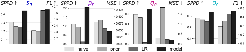
Figure 4: Intrinsic evaluation on the held-out set: we impute removed values $y_{n}$, e.g., $\{{\color[rgb]{0.5234375,0.046875,0.76171875}p_{n}}\}$, of one site based on values $y_{n}^{\text{remain}}$ of remaining sites, e.g., $\{{\color[rgb]{0.046875,0.0703125,0.76171875}s_{n}},{\color[rgb]{0.76171875,0.046875,0.5234375}q_{n}},{\color[rgb]{0.046875,0.703125,0.76171875}o_{n}}\}$. We present mean results of scaled pointwise predictive density (SPPD) and error metrics (weighted F1 / MSE) over $5$ runs. We compare three variants of our model with $C=5$ latent classes: a naive baseline fitted only to the single site that is removed at test time; an unfitted version, whose parameters are randomly drawn from the prior, and a fitted variant of the proposed model. In addition, we train four linear regression (LR) models to directly predict $y_{n}$ from $y_{n}^{\text{remain}}$.

5 Intrinsic Evaluation: Imputation

To evaluate the fit of our model, we conduct a series of predictive experiments. We randomly split the $N=$112089$$ events into a $70$% training and $30$% held-out set. We fit the model on the training set $X$ and approximate the posterior distribution of continuous parameters $\theta$ based on $T=$1000$$ NUTS samples after discarding the first $200$ burn-in samples. For evaluation on the held-out set $Y$, we report scaled pointwise predictive density (SPPD), mean squared error and weighted F1 score as detailed in App. A.

5.1 Number of Latent Classes $C$

The number of classes $C$ that our latent variable $z_{n}$ ranges over can be regarded a hyperparameter. To identify the optimal setting of $C$, we repeatedly fit the model on the training set and evaluate it on the held-out set. We do so for each class setting in $C=[3,\ldots,7]$ and find that $C=5$ yields the best model fit overall, as shown in Fig. 3.

5.2 Imputation Task

Procedure.

Next, we conduct a data imputation task. On the held-out set, we remove one observed site from all event tuples and refer to it as $y_{n}$ — e.g., we remove all Goldstein values and obtain $y_{n}=\{{\color[rgb]{0.5234375,0.046875,0.76171875}p_{n}}\}$. We use the remaining three-way event tuples $y_{n}^{\text{remain}}=\{{\color[rgb]{0.046875,0.0703125,0.76171875}s_{n}},{\color[rgb]{0.76171875,0.046875,0.5234375}q_{n}},{\color[rgb]{0.046875,0.703125,0.76171875}o_{n}}\}$ jointly with the posterior of $\theta$ to make predictions of $y_{n}$. In particular, we draw samples from the posterior predictive distribution $\widehat{y}_{n}^{(t)}\sim p(y_{n}\mid\theta^{(t)},y_{n}^{\text{remain}})$ and compute their mean $\widehat{y}_{n}=\frac{1}{T}\sum_{t=1}^{T}\widehat{y}_{n}^{(t)}$ to get point estimates of $y_{n}$.

Baselines.

We compare the proposed model against three baselines, where the first two baselines are simple and we expect our proposed model to outperform them. For the first baseline, we fit four versions of the proposed model to only one of the observed sites $\{{\color[rgb]{0.046875,0.0703125,0.76171875}s_{n}},{\color[rgb]{0.5234375,0.046875,0.76171875}p_{n}},{\color[rgb]{0.76171875,0.046875,0.5234375}q_{n}},{\color[rgb]{0.046875,0.703125,0.76171875}o_{n}}\}$. This naive baseline effectively just learns the empirical histogram of each site in the training set, and uses the relevant one to make predictions for $y_{n}$ — we refer to this as naive. For the second baseline, we use an unfitted version of the proposed model, whose parameters have been sampled from the prior. For the last baseline, we train four linear regression models (LR) to predict $y_{n}$ directly from $y_{n}^{\text{remain}}$.

Results.

Fig. 4 reports the results of the imputation experiments, where the proposed model performs comparatively well, obtaining substantially better predictive performance over both the naive and non-naive baselines.

	forecasting Goldstein time series ${\color[rgb]{0.5234375,0.046875,0.76171875}\bar{\boldsymbol{p}}_{\ell}}$					forecasting casualty count time series ${\color[rgb]{0.76171875,0.046875,0.5234375}\bar{\boldsymbol{q}}_{\ell}}$
	${\color[rgb]{0.5234375,0.046875,0.76171875}\bar{\boldsymbol{p}}_{\ell}}\xrightarrow{}{\color[rgb]{0.5234375,0.046875,0.76171875}\bar{\boldsymbol{p}}_{\ell}}$	${\color[rgb]{0.5234375,0.046875,0.76171875}\bar{\boldsymbol{p}}_{\ell}},{\color[rgb]{0.76171875,0.046875,0.5234375}\bar{\boldsymbol{q}}_{\ell}}\xrightarrow{}{\color[rgb]{0.5234375,0.046875,0.76171875}\bar{\boldsymbol{p}}_{\ell}}$		${\color[rgb]{0.5234375,0.046875,0.76171875}\bar{\boldsymbol{p}}_{\ell}},\bar{\boldsymbol{z}}_{\ell}\xrightarrow{}{\color[rgb]{0.5234375,0.046875,0.76171875}\bar{\boldsymbol{p}}_{\ell}}$		${\color[rgb]{0.76171875,0.046875,0.5234375}\bar{\boldsymbol{q}}_{\ell}}\xrightarrow{}{\color[rgb]{0.76171875,0.046875,0.5234375}\bar{\boldsymbol{q}}_{\ell}}$	${\color[rgb]{0.5234375,0.046875,0.76171875}\bar{\boldsymbol{p}}_{\ell}},{\color[rgb]{0.76171875,0.046875,0.5234375}\bar{\boldsymbol{q}}_{\ell}}\xrightarrow{}{\color[rgb]{0.76171875,0.046875,0.5234375}\bar{\boldsymbol{q}}_{\ell}}$		${\color[rgb]{0.76171875,0.046875,0.5234375}\bar{\boldsymbol{q}}_{\ell}},\bar{\boldsymbol{z}}_{\ell}\xrightarrow{}{\color[rgb]{0.76171875,0.046875,0.5234375}\bar{\boldsymbol{q}}_{\ell}}$
country $\ell$	MSE	MSE	Grang	MSE	Grang	MSE	MSE	Grang	MSE	Grang
Egypt	3.33	3.15	0.30	3.14	0.19	0.22	0.15	0.79	0.14	0.35
Iraq	4.85	4.82	0.05	4.82	0.05	2.91	2.82	0.05	2.82	0.14
Syria	2.96	3.10	0.29	3.10	0.35	0.56	0.49	0.28	0.50	0.10
Yemen	5.09	5.12	0.15	5.12	0.46	1.41	1.02	0.15	1.02	0.02

Table 2: Forecasting: we test how much predictive information our intensity time series $\bar{\boldsymbol{z}}_{\ell}$ holds on future developments of Goldstein values ${\color[rgb]{0.5234375,0.046875,0.76171875}\bar{\boldsymbol{p}}_{\ell}}$ and casualty counts ${\color[rgb]{0.76171875,0.046875,0.5234375}\bar{\boldsymbol{q}}_{\ell}}$. In most cases, the vector autoregression (VAR) outperforms the autoregression in terms of mean squared error (MSE) (results reported are $10^{-1}$) on the held-out set. We find that $\bar{\boldsymbol{z}}_{\ell}$ holds information on both ${\color[rgb]{0.5234375,0.046875,0.76171875}\bar{\boldsymbol{p}}_{\ell}}$ and ${\color[rgb]{0.76171875,0.046875,0.5234375}\bar{\boldsymbol{q}}_{\ell}}$ as including $\bar{\boldsymbol{z}}_{\ell}$ as an additional time series performs en par with including ${\color[rgb]{0.5234375,0.046875,0.76171875}\bar{\boldsymbol{p}}_{\ell}}$ or ${\color[rgb]{0.76171875,0.046875,0.5234375}\bar{\boldsymbol{q}}_{\ell}}$ throughout the VAR experiments. If the $p$ value of the corresponding Granger (Grang) test is small, we can reject the null hypothesis that the additional time series does not add predictive information.

6 Extrinsic Evaluation: Time Series

In the last section, we intrinsically evaluated the proposed model by having it impute held-out data. In this section, we consider extrinsic evaluations of the proposed model, which seek to evaluate it on downstream predictive tasks for which it was not explicitly designed. In this section, we rely on features of events coded by NAVCO which our model does not access during training. In particular, NAVCO codes for the location $\ell_{n}$ and the timestamp $\tau_{n}$ of each event. We discretize time so that each event is associated with a specific month $m_{n}$. Augmented with these extra characteristics, as well as with the mean intensity inferred by our model, each event $n$ has the following attributes: $\{{\color[rgb]{0.046875,0.0703125,0.76171875}s_{n}},{\color[rgb]{0.5234375,0.046875,0.76171875}p_{n}},{\color[rgb]{0.76171875,0.046875,0.5234375}q_{n}},{\color[rgb]{0.046875,0.703125,0.76171875}o_{n}},\ell_{n},m_{n},\bar{z}_{n}\}$. In all of the tasks in this section, we split events according to their location $\ell_{n}=\ell$ and examine monthly-aggregated time series of the cardinal and ordinal quantities $\{{\color[rgb]{0.5234375,0.046875,0.76171875}p_{n}},{\color[rgb]{0.76171875,0.046875,0.5234375}q_{n}},\bar{z}_{n}\}$. In particular, we ask two questions: 1) whether $\bar{z}_{n}$ adds predictive information for forecasting ${\color[rgb]{0.5234375,0.046875,0.76171875}p_{n}}$ and ${\color[rgb]{0.76171875,0.046875,0.5234375}q_{n}}$, and 2) whether the model-based measure of intensity $\bar{z}_{n}$ correlates with Google Trends more than just ${\color[rgb]{0.5234375,0.046875,0.76171875}p_{n}}$ and ${\color[rgb]{0.76171875,0.046875,0.5234375}q_{n}}$.

Event Time Series.

We construct time series in the following way. We first run inference on a training dataset $X$ to obtain posterior samples of the parameters $\{\theta^{(t)}\}_{t=1}^{T}$. We then use the trained parameters to obtain intensity scores $\{\boldsymbol{z}^{(t)}\}_{t=1}^{T}$ for both events in the training set as well as events in a test set that the model did not access. We then compute $\bar{z}_{n}$ for each $n$ and re-scale the $\bar{z}_{n}$ estimates to cover a $[0,1]$ range as we did with Goldstein values. For each location $\ell$ and month $m$ appearing in the data, we then construct the posterior average intensity class $\bar{z}_{\ell,m}$:

$$\bar{z}_{\ell,m}=\frac{\sum_{n=1}^{N}\bar{z}_{n}\,\mathbbm{1}(\ell_{n}=\ell)\mathbbm{1}(m_{n}=m)}{\sum_{n=1}^{N}\mathbbm{1}(\ell_{n}=\ell)\mathbbm{1}(m_{n}=m)}$$ (13)

For a given location $\ell$, we refer to the full time series over months as $\bar{\boldsymbol{z}}_{\ell}$ and linearly interpolate the entries $m$ corresponding to months for which there is no data. We similarly aggregate the observed sites per event to obtain time series of predicates ${\color[rgb]{0.5234375,0.046875,0.76171875}\bar{\boldsymbol{p}}_{\ell}}$ and quantifiers ${\color[rgb]{0.76171875,0.046875,0.5234375}\bar{\boldsymbol{q}}_{\ell}}$.

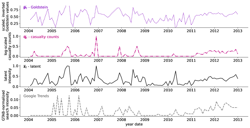
Figure 5: Time series of events in Syria between 2004 and 2013, all values averaged by month. We observe that our intensity time series $\bar{\boldsymbol{z}}_{\ell}$ smoothly interpolates between the Goldstein ${\color[rgb]{0.5234375,0.046875,0.76171875}\bar{\boldsymbol{p}}_{\ell}}$ and casualty counts time series ${\color[rgb]{0.76171875,0.046875,0.5234375}\bar{\boldsymbol{q}}_{\ell}}$. We look at Google trends as an external correlate for (perceived) conflict intensity and report correlations in Fig. 6.

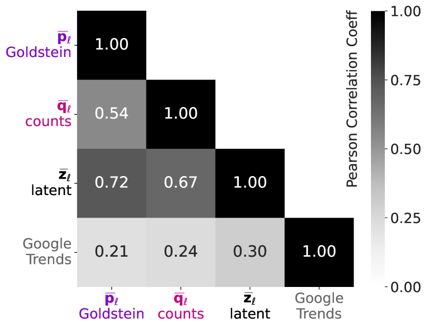
Figure 6: Pearson correlation between time series displayed in Fig. 5. Our latent intensity time series $\bar{\boldsymbol{z}}_{\ell}$ is positively correlated with the Goldstein ${\color[rgb]{0.5234375,0.046875,0.76171875}\bar{\boldsymbol{p}}_{\ell}}$ and casualty counts time series ${\color[rgb]{0.76171875,0.046875,0.5234375}\bar{\boldsymbol{q}}_{\ell}}$. Google trends are more strongly correlated with $\bar{\boldsymbol{z}}_{\ell}$ than with ${\color[rgb]{0.5234375,0.046875,0.76171875}\bar{\boldsymbol{p}}_{\ell}}$ and ${\color[rgb]{0.76171875,0.046875,0.5234375}\bar{\boldsymbol{q}}_{\ell}}$.

Autoregressive Forecasting.

Does knowledge of the inferred intensity time series $\bar{\boldsymbol{z}}_{\ell}$ improve forecasting of the Goldstein ${\color[rgb]{0.5234375,0.046875,0.76171875}\bar{\boldsymbol{p}}_{\ell}}$ and casualty count ${\color[rgb]{0.76171875,0.046875,0.5234375}\bar{\boldsymbol{q}}_{\ell}}$ time series? To test this, we first consider autoregressive (AR) models that forecast monthly values of each time series (e.g., ${\color[rgb]{0.5234375,0.046875,0.76171875}\bar{p}_{\ell,m}}$) based on the previous values of only that same time series (e.g., ${\color[rgb]{0.5234375,0.046875,0.76171875}\boldsymbol{\bar{p}}_{\ell,1:(m-1)}}$). We then consider vector autoregressive (VAR) models that use multiple time series (e.g., ${\color[rgb]{0.5234375,0.046875,0.76171875}\boldsymbol{\bar{p}}_{\ell,1:(m-1)}}$ and ${\color[rgb]{0.76171875,0.046875,0.5234375}\boldsymbol{\bar{q}}_{\ell,1:(m-1)}}$) to form the same predictions. When incorporating values from our latent intensity time series $\bar{\boldsymbol{z}}_{\ell}$, we must be careful to avoid test set leakage. To do so, we fit our model to a subset of data $X_{\backslash\ell}$ that excludes any events in a particular location $\ell$. We obtain posterior samples $\{\theta^{(t)}_{\backslash\ell}\}_{t=1}^{T}$ by fitting the proposed model to $X_{\backslash\ell}$. We then use these parameters to obtain $\bar{z}_{n}$ for all events $n$ in both the training $X_{\backslash\ell}$ and test set $X_{\ell}$.

Before fitting any (vector) autoregressive models and performing the forecasting experiments, we apply a first-order differencing transform to all time series to remove potential linear trends, and verify each time series’ stationarity using an Augmented Dickey-Fuller test (Fuller, 1976). We then fit an autoregressive (AR) model to each individual time-series and a vector autoregressive (VAR) model to all pairs of time series. We determine their optimal orders (lag) in months using Bayesian Information Criterion (BIC), and use cross validation to measure held-out forecasting error across 24 folds. In Tab. 2, we report results in mean squared error (MSE) on the held-out sets averaged over all $24$ folds. Indeed, our results suggest that $\bar{\boldsymbol{z}}_{\ell}$ contains (predictive) information on both ${\color[rgb]{0.5234375,0.046875,0.76171875}\bar{\boldsymbol{p}}_{\ell}}$ and ${\color[rgb]{0.76171875,0.046875,0.5234375}\bar{\boldsymbol{q}}_{\ell}}$. For instance, in the VAR experiments for forecasting ${\color[rgb]{0.5234375,0.046875,0.76171875}\bar{\boldsymbol{p}}_{\ell}}$, we may replace the additional time series ${\color[rgb]{0.76171875,0.046875,0.5234375}\bar{\boldsymbol{q}}_{\ell}}$ with $\bar{\boldsymbol{z}}_{\ell}$ without any drop in performance. We also report Granger tests (Granger, 1969) which test the null hypothesis that forecasting a variable (e.g., ${\color[rgb]{0.5234375,0.046875,0.76171875}\bar{\boldsymbol{p}}_{\ell}}$) using only its own history is no less accurate than also using an additional variable’s history (e.g., $\bar{\boldsymbol{z}}_{\ell}$).

Descriptive Analysis.

A growing body of work analyzes the correlation between shifts in online behavior or media attention and conflict intensity (Chykina and Crabtree, 2018; Timoneda and Wibbels, 2022). Following this line of work, we download time series of Google search keywords using the Google Trends Anchorbank (G-TAB) (West, 2020). We constrain searches to the category of “World News” and use the country name of location $\ell$ as the search keyword. In contrast to the forecasting setting, we fit our model to the entire dataset $X$, including events associated with the respective location, and obtain an intensity time series $\bar{\boldsymbol{z}}_{\ell}$. Fig. 5 shows a comparison between four time series: the Goldstein ${\color[rgb]{0.5234375,0.046875,0.76171875}\bar{\boldsymbol{p}}_{\ell}}$, casualty counts ${\color[rgb]{0.76171875,0.046875,0.5234375}\bar{\boldsymbol{q}}_{\ell}}$, our latent $\bar{\boldsymbol{z}}_{\ell}$ and the Google trends time series for Syria between 2004 and 2013. We observe that $\bar{\boldsymbol{z}}_{\ell}$ nicely interpolates between the time series of ${\color[rgb]{0.5234375,0.046875,0.76171875}\bar{\boldsymbol{p}}_{\ell}}$ and ${\color[rgb]{0.76171875,0.046875,0.5234375}\bar{\boldsymbol{q}}_{\ell}}$. It captures larger trends and fluctuations in both time series, while not exactly mirroring either. Further, in Fig. 6, we report Pearson correlation coefficients between all pairs of time series. While ${\color[rgb]{0.5234375,0.046875,0.76171875}\bar{\boldsymbol{p}}_{\ell}}$ and ${\color[rgb]{0.76171875,0.046875,0.5234375}\bar{\boldsymbol{q}}_{\ell}}$ are positively correlated, ${\color[rgb]{0.5234375,0.046875,0.76171875}\bar{\boldsymbol{p}}_{\ell}}$ is more strongly correlated with $\bar{\boldsymbol{z}}_{\ell}$ than with ${\color[rgb]{0.76171875,0.046875,0.5234375}\bar{\boldsymbol{q}}_{\ell}}$. Moreover, Google trends are more strongly correlated with $\bar{\boldsymbol{z}}_{\ell}$ than either ${\color[rgb]{0.5234375,0.046875,0.76171875}\bar{\boldsymbol{p}}_{\ell}}$ or ${\color[rgb]{0.76171875,0.046875,0.5234375}\bar{\boldsymbol{q}}_{\ell}}$. We hypothesize this may be due to the additional information on the subject ${\color[rgb]{0.046875,0.0703125,0.76171875}s_{n}}$ and object types ${\color[rgb]{0.046875,0.703125,0.76171875}o_{n}}$ that $z_{n}$ encodes, and which may contribute to how much attention is paid to different conflicts, as measured by Google Trends.

7 Related Work

There are a number of relevant papers that broadly seek to measure “latent concepts” (Douglass et al., 2022) pertaining to international relations, particularly using event data. Terechshenko (2020) uses a Bayesian item-response theory model to learn ordinal conflict intensity levels from observed event types. O’Connor et al. (2013) present an unsupervised, probabilistic topic model to learn an ontology of event data and use the Goldstein scale to evaluate it. Schein et al. (2015, 2016, 2019) decompose four-way tensors (senders, receivers, actions, time steps) to infer latent classes of CAMEO-coded events. Stoehr et al. (2023b) build on those models by further imposing an ordering on their latent space, which captures conflict–cooperation intensity. Another line of work models friend–enemy relationship trajectories using neural network-based (Han et al., 2019) or hidden Markov model-based (Chaturvedi et al., 2017) approaches. There also exists work on signed network representations of relationships that are extracted from text (Srivastava et al., 2016; Choi et al., 2016) or Wikipedia conflict articles (Stoehr et al., 2021).

8 Future Work

Assuming civilian casualties are “more intense” than military casualties, we could impose an additional ordering on object types ${\color[rgb]{0.046875,0.703125,0.76171875}o_{n}}$. We could also condition observed sites on each other—e.g., casualty counts ${\color[rgb]{0.76171875,0.046875,0.5234375}q_{n}}$ are conditionally dependent on ${\color[rgb]{0.046875,0.703125,0.76171875}o_{n}}$ or even ${\color[rgb]{0.5234375,0.046875,0.76171875}p_{n}}$ under the model. We plan to further incorporate multiple latent variables to model multi-dimensional intensity concepts. Future models could also condition on location and include a temporal component to account for how surprisal may affect the perceived intensity of an event. We also note that the latent variable model presented in this work could also be extended to a more general framework for learning interpretable, ordinal scales from a set of mixed-type data that include cardinal or ordinal observations. We plan to explore generalizations of the proposed model and applications beyond of international relations.

Limitations

We discuss limitations of our modeling assumptions in § 8. They are based on prior work in political science such as the CAMEO ontology and the Goldstein scale. On this account, they may replicate or potentially introduce biases. Hyperparameter search, settings and implementation details are provided in § 4.2 and § 5. All NAVCO event descriptions are limited to English language, but do not disclose individuals.

Impact Statement

We emphasize that our models are intended for research, analysis and monitoring purposes. They should not be blindly deployed for automatized decision-making processes. The notion of conflict intensity is intrinsically hard to quantify: it is strongly dependent on socio-cultural background and subjective experience.

Appendix A Evaluation Metrics

To evaluate the posterior predictive distribution $p(y_{n}\mid\theta^{(t)})$, we consider a scaled variant of the log pointwise predictive density (LPPD; Gelman et al., 1996, 2014), which we term SPPD:

$$\exp\left({\frac{1}{N}\sum_{n=1}^{N}\log\big{(}\frac{1}{T}\sum_{t=1}^{T}p(y_{n}\mid\theta^{(t)})\big{)}}\right)$$ (14)

The term inside the log, $\frac{1}{T}\sum_{t=1}^{T}p(y_{n}\mid\theta^{(t)})$, computes a Monte Carlo approximation to the posterior predictive density for a given $y_{n}$. The rest, $\exp\left({\frac{1}{N}\sum_{n=1}^{N}\log(\cdot)}\right)$, then computes the geometric mean of the pointwise densities.

We also compute point estimates via the posterior predictive mean $\frac{1}{T}\sum_{t=1}^{T}{\mathbb{E}}[y_{n}\mid\theta^{(t)}]$ which allows comparing predicted and true values based on error metrics like weighted F1 score or mean-squared error (MSE).

Appendix B Inverse of the Ordered Normal

We define the Ordered Normal distribution with the help of an ordering transformation in eq. 8. This transformation is a smooth bijection since its inverse is given by:

$$x_{c}\leftarrow\begin{cases}\lambda_{1}&\text{if }c=1\\ \log(\lambda_{c}-\lambda_{c-1})&\text{if }c>1\end{cases}$$ (15)

Note that for all $c$, $\lambda_{c}>\lambda_{c-1}$, so the $\log$ is well-defined.

CAMEO actor code	meaning	group 4 mapping
REB	rebels	military
MIL	military	military
GOV	government	government
ETH	ethnic	civilian
REL	religious	civilian
COP	police forces	military
JUD	judiciary	political
OPP	political opposition	political
LLY	regime loyalists	government
ACT	activists	political
NON	non-aligned third party	military
SPY	state intelligence	military
UAF	unidentified armed forces	military
UNS	unidentified unarmed non-state actors	civilian
NGO	non-governmental organisation	political
BUS	business	civilian
CVL	civilian group	civilian
IND	civilian individual	civilian
EDU	educators	civilian
STU	students	civilian
YTH	youth	civilian
ELI	elites	civilian
LAB	labour	civilian
LEG	legislature	political
PTY	political party	political
MED	media	civilian
REF	refugees	civilian
IGO	inter-governmental	political
NGM	non-governmental movement	political
MNC	multinational cooperation	civilian
INT	international actors	political
TOP	top officials	political
MID	mid-lower level officials	political
HAR	hardliners	political
MOD	moderates	political

Table 3: CAMEO actor types to group 4 mapping. The NAVCO columns “actor3”, “actor6” and “target3”, “target6” correspond to actor types defined by the CAMEO actor codebook. We consider $33$ generic CAMEO actor types and map them into one of the $4$ classes “civilian”, “military”, “governmental” and “political”.

References

- Beieler (2016) John Beieler. 2016. Creating a real-time, reproducible event dataset. arXiv, 1612.00866.
- Bingham et al. (2018) Eli Bingham, Jonathan P. Chen, Martin Jankowiak, Fritz Obermeyer, Neeraj Pradhan, Theofanis Karaletsos, Rohit Singh, Paul Szerlip, Paul Horsfall, and Noah D. Goodman. 2018. Pyro: Deep universal probabilistic programming. Journal of Machine Learning Research.
- Bond et al. (2003) Doug Bond, Joe Bond, Churl Oh, Craig Jenkins, and Charles Lewis Taylor. 2003. Integrated data for events analysis (IDEA): An event typology for automated events data development. Journal of Peace Research, 40(6):733–745.
- Boschee et al. (2015) Elizabeth Boschee, Jennifer Lautenschlager, Sean O’Brien, Steve Shellman, James Starz, and Michael Ward. 2015. ICEWS coded event data.
- Chaturvedi et al. (2017) Snigdha Chaturvedi, Mohit Iyyer, and Hal Daume III. 2017. Unsupervised learning of evolving relationships between literary characters. Proceedings of the AAAI Conference on Artificial Intelligence, 31(1).
- Chaudoin et al. (2017) Stephen Chaudoin, Zachary Peskowitz, and Christopher Stanton. 2017. Beyond zeroes and ones: The intensity and dynamics of civil conflict. The Journal of Conflict Resolution, 61(1):56–83.
- Chenoweth et al. (2018) Erica Chenoweth, Jonathan Pinckney, and Orion Lewis. 2018. Days of rage: Introducing the NAVCO 3.0 dataset. Journal of Peace Research, 55(4):524–534.
- Choi et al. (2016) Eunsol Choi, Hannah Rashkin, Luke Zettlemoyer, and Yejin Choi. 2016. Document-level sentiment inference with social, faction, and discourse context. In Proceedings of the 54th Annual Meeting of the Association for Computational Linguistics, pages 333–343.
- Chykina and Crabtree (2018) Volha Chykina and Charles Crabtree. 2018. Using Google trends to measure issue salience for hard-to-survey populations. Socius: Sociological Research for a Dynamic World, 4:237802311876041.
- Douglass et al. (2022) Rex Douglass, Thomas Leo Scherer, Andrés Gannon, Erik Gartzke, Jon Lindsay, Shannon Carcelli, Jonathan Wilkenfeld, David M. Quinn, Catherine Aiken, Jose Miguel Cabezas Navarro, Neil Lund, Egle Murauskaite, and Diana Partridge. 2022. Introducing the ICBe dataset: Very high recall and precision event extraction from narratives about international crises. arXiv, 2202.07081.
- Fisher (2012) Max Fisher. 2012. Google trends: The moment Syria’s ‘revolution’ became a ‘civil war’. Washington Post.
- Fuller (1976) Wayne A. Fuller. 1976. Introduction to Statistical Time Series. Wiley.
- Gelman et al. (2014) Andrew Gelman, Jessica Hwang, and Aki Vehtari. 2014. Understanding predictive information criteria for Bayesian models. Statistics and Computing, 24(6):997–1016.
- Gelman et al. (1996) Andrew Gelman, Xiao-Li Meng, and Hal Stern. 1996. Posterior predictive assessment of model fitness via realized discrepancies. Statistica Sinica, 6(4):733–760.
- Goldstein (1992) Joshua Goldstein. 1992. A conflict-cooperation scale for WEIS events data. The Journal of Conflict Resolution, 36(2):369–385.
- Granger (1969) Clive Granger. 1969. Investigating causal relations by econometric models and cross-spectral methods. Econometrica, 37(3):424–438.
- Han et al. (2019) Xiaochuang Han, Eunsol Choi, and Chenhao Tan. 2019. No permanent friends or enemies: Tracking relationships between nations from news. In Proceedings of the 2019 Conference of the North American Chapter of the Association for Computational Linguistics, volume 1, pages 1660–1676.
- Homan and Gelman (2014) Matthew D. Homan and Andrew Gelman. 2014. The No-U-Turn Sampler: Adaptively setting path lengths in Hamiltonian Monte Carlo. Journal of Machine Learning Research, 15(1):1593–1623.
- King and Lowe (2003) Gary King and Will Lowe. 2003. An automated information extraction tool for international conflict data with performance as good as human coders: A rare events evaluation design. International Organization, 57(3):617–642.
- Leetaru and Schrodt (2013) Kalev Leetaru and Philip Schrodt. 2013. GDELT: Global data on events, location, and tone. In ISA Annual Convention.
- Lewis et al. (2016) Orion A. Lewis, Erica Chenoweth, and Jonathan Pinckney. 2016. Nonviolent and violent campaigns and outcomes 3.0: Effects of tactical choices on strategic outcomes codebook.
- McClelland (1984) Charles McClelland. 1984. World event/interaction survey (WEIS) project, 1966-1978: Archival version.
- O’Connor et al. (2013) Brendan O’Connor, Brandon Stewart, and Noah Smith. 2013. Learning to extract international relations from political context. In Proceedings of the 51st Annual Meeting of the Association for Computational Linguistics, volume 1, pages 1094–1104.
- Schein et al. (2019) Aaron Schein, Scott W. Linderman, Mingyuan Zhou, David M. Blei, and Hanna Wallach. 2019. Poisson-randomized gamma dynamical systems. In Advances in Neural Information Processing Systems.
- Schein et al. (2015) Aaron Schein, John Paisley, David M. Blei, and Hanna Wallach. 2015. Bayesian Poisson tensor factorization for inferring multilateral relations from sparse dyadic event counts. In Proceedings of the 21th ACM SIGKDD International Conference on Knowledge Discovery and Data Mining, pages 1045–1054.
- Schein et al. (2016) Aaron Schein, Mingyuan Zhou, David M. Blei, and Hanna Wallach. 2016. Bayesian Poisson Tucker decomposition for learning the structure of international relations. In Proceedings of the 33rd International Conference on Machine Learning, volume 48, pages 2810–2819.
- Schrodt (2008) Philip Schrodt. 2008. Kansas event data system (KEDS). In AAAS Center for Scientific Responsibility and Justice.
- Schrodt (2012) Philip Schrodt. 2012. CAMEO: Conflict and mediation event observations event and actor codebook. Parus Analytics.
- Schrodt (2019) Philip Schrodt. 2019. Stuff I tell people about event data.
- Srivastava et al. (2016) Shashank Srivastava, Snigdha Chaturvedi, and Tom Mitchell. 2016. Inferring interpersonal relations in narrative summaries. In Proceedings of the Thirtieth AAAI Conference on Artificial Intelligence, pages 2807–2813.
- Stephens (2000) Matthew Stephens. 2000. Dealing with label switching in mixture models. Journal of the Royal Statistical Society: Series B (Statistical Methodology), 62(4):795–809.
- Stoehr et al. (2023a) Niklas Stoehr, Ryan Cotterell, and Aaron Schein. 2023a. Sentiment as an ordinal latent variable. In Proceedings of the 17th Conference of the European Chapter of the Association for Computational Linguistics.
- Stoehr et al. (2021) Niklas Stoehr, Lucas Torroba Hennigen, Samin Ahbab, Robert West, and Ryan Cotterell. 2021. Classifying dyads for militarized conflict analysis. In Proceedings of the 2021 Conference on Empirical Methods in Natural Language Processing (EMNLP).
- Stoehr et al. (2023b) Niklas Stoehr, Benjamin J. Radford, Ryan Cotterell, and Aaron Schein. 2023b. The Ordered Matrix Dirichlet for state-space models. In Proceedings of The 26th International Conference on Artificial Intelligence and Statistics.
- Terechshenko (2020) Zhanna Terechshenko. 2020. Hot under the collar: A latent measure of interstate hostility. Journal of Peace Research, 57(6):764–776.
- Timoneda and Wibbels (2022) Joan C. Timoneda and Erik Wibbels. 2022. Spikes and variance: Using Google trends to detect and forecast protests. Political Analysis, 30(1):1–18.
- West (2020) Robert West. 2020. Calibration of Google trends time series. Proceedings of the 29th ACM International Conference on Information & Knowledge Management, pages 2257–2260.
- Zhong et al. (2023) Mian Zhong, Shehzaad Dhuliawala, and Niklas Stoehr. 2023. Extracting victim counts from text. In Proceedings of the 17th Conference of the European Chapter of the Association for Computational Linguistics.