Asymptotically Unbiased Instance-wise Regularized Partial AUC Optimization: Theory and Algorithm

Abstract

The Partial Area Under the ROC Curve (PAUC), typically including One-way Partial AUC (OPAUC) and Two-way Partial AUC (TPAUC), measures the average performance of a binary classifier within a specific false positive rate and/or true positive rate interval, which is a widely adopted measure when decision constraints must be considered. Consequently, PAUC optimization has naturally attracted increasing attention in the machine learning community within the last few years. Nonetheless, most of the existing methods could only optimize PAUC approximately, leading to inevitable biases that are not controllable. Fortunately, a recent work presents an unbiased formulation of the PAUC optimization problem via distributional robust optimization. However, it is based on the pair-wise formulation of AUC, which suffers from the limited scalability w.r.t. sample size and a slow convergence rate, especially for TPAUC. To address this issue, we present a simpler reformulation of the problem in an asymptotically unbiased and instance-wise manner. For both OPAUC and TPAUC, we come to a nonconvex strongly concave minimax regularized problem of instance-wise functions. On top of this, we employ an efficient solver enjoys a linear per-iteration computational complexity w.r.t. the sample size and a time-complexity of $O(\epsilon^{-1/3})$ to reach a $\epsilon$ stationary point. Furthermore, we find that the minimax reformulation also facilitates the theoretical analysis of generalization error as a byproduct. Compared with the existing results, we present new error bounds that are much easier to prove and could deal with hypotheses with real-valued outputs. Finally, extensive experiments on several benchmark datasets demonstrate the effectiveness of our method.

1 Introduction

AUC refers to the Area Under the Receiver Operating Characteristic (ROC) curve [1], where the ROC curve is obtained by plotting the True Positive Rate (TPR) against the False Positive Rate (FPR) of a given classifier for all possible thresholds. Since it is insensitive to the class distribution, AUC has become one of the standard metrics for long-tail, and imbalanced datasets [1, 22, 38]. Consequently, AUC optimization has attracted increasing attention in the machine learning community ever since the early 2000s [13, 5, 35, 17]. Over the last two decades, research on AUC optimization has evolved from the simplest linear models and decision trees [27, 10, 29, 41] to state-of-the-art deep learning architectures [21, 14, 37, 43, 42, 33]. With such remarkable success, one can now easily apply AUC optimization to deal with various real-world problems ranging from financial fraud detection[16, 4, 23], spam email detection [24], to medical diagnosis [24, 38, 37, 43], etc.

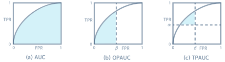
Figure 1: The comparison among different AUC variants. (a) The area under the ROC curve (AUC). (b) The one-way partial AUC (OPAUC). (c) The two-way partial AUC (TPAUC).

However, in such long-tailed applications, we are often interested in a specific region in the ROC curve where its area is called Partial AUC (PAUC). As illustrated in Fig.1, there are two types of PAUC. Here, One-way Partial AUC (OPAUC) measures the area within an FPR interval ( $0\leq\mathrm{FPR}\leq\beta$); while Two-way Partial AUC (TPAUC) measures the area with $\mathrm{FPR}\leq\beta$, $\mathrm{TPR}\geq\alpha$. Unlike the full AUC, optimizing PAUC requires selecting top-ranked or/and bottom-ranked instances, leading to a hard combinatorial optimization problem. Many efforts have been made to solve the problem [6, 24, 25, 20, 39]. However, the majority of them rely on full-batch optimization and the approximation of the top (bottom)-$k$ ranking process, which suffers from immeasurable biases and undesirable efficiency. Most recently, researchers have started to explore mini-batch PAUC optimization for deep learning models. [39] proposed a novel end-to-end optimization framework for PAUC. This formulation has a fast convergence rate with the help of a stochastic optimization algorithm, but the estimation of PAUC is still biased. Later, [44] proposed a Distributional Robust Optimization (DRO) framework for PAUC optimization, where the bias can be eliminated by a clever reformulation and the compositional SGD algorithms [28]. However, they adopt the pair-wise loss function which has limited scalability w.r.t. sample size and $O(\epsilon^{-4})$/$O(\epsilon^{-6})$ time complexity to reach the $\epsilon$-stationary point for $\mathrm{OPAUC}$/$\mathrm{TPAUC}$. Considering the efficiency bottleneck comes from the pair-wise formulation, we will explore the following question in this paper:

To answer this question, we propose an efficient and nearly unbiased optimization algorithm (the bias vanishes asymptotically when $\kappa\rightarrow 0$) for regularized PAUC maximization with a faster convergence guarantee. The comparison with previous results are listed in Tab.1. We consider both $\mathrm{OPAUC}$ and $\mathrm{TPAUC}$ maximization, where for $\mathrm{OPAUC}$, we focus on maximizing PAUC in the region: $\mathrm{FPR}\leq\beta$ and for $\mathrm{TPAUC}$ we focus on the region: $\mathrm{FPR}\leq\beta$ and $\mathrm{TPR}\geq\alpha$. We summarize our contributions below.

Table 1: Comparison with existing partial AUC algorithms. The convergence rate represents the number of iterations after which an algorithm can find an $\epsilon$-stationary point, where $\epsilon$-sp is $\epsilon$-stationary point. $\triangle$ implies a natural result of non-convex SGD. $n_{+}^{B}$ ($n_{-}^{B}$ resp.) is the number of positive (negative resp.) instances for each mini-batch $B$.

	SOPA [44]	SOPA-S [44]	TPAUC [39]	Ours
Convergence Rate ($\mathrm{OPAUC}$)	$O(\epsilon^{-4})$	$O(\epsilon^{-4})$	$O(\epsilon^{-4})^{\triangle}$	$O(\epsilon^{-3})$
Convergence Rate ($\mathrm{TPAUC}$)	$O(\epsilon^{-6})$	$O(\epsilon^{-4})$	$O(\epsilon^{-4})^{\triangle}$	$O(\epsilon^{-3})$
Convergence Measure	$\epsilon$-sp (non-smooth)	$\epsilon$-sp	$\epsilon$-sp	$\epsilon$-sp
Smoothness	non-smooth	smooth	smooth	smooth
Unbiasedness	$\surd$	$\times$	$\times$	with bias $O(1/\kappa)$ when $\omega=0$
Per-Iteration Time Complexity	$O(n_{+}^{B}n_{-}^{B})$	$O(n_{+}^{B}n_{-}^{B})$	$O(n_{+}^{B}n_{-}^{B})$	$O(n_{+}^{B}+n_{-}^{B})$

• With a proper regularization, we propose a nonconvex strongly concave minimax instance-wise formulation for $\mathrm{OPAUC}$ and $\mathrm{TPAUC}$ maximization. On top of our proposed formulation, we employ an efficient stochastic minimax algorithm that finds a $\epsilon$-stationary point within $O(\epsilon^{-3})$ iterations.

• We conduct a generalization analysis of our proposed methods. Our instance-wise reformulation can overcome the interdependent issue of the original pair-wise generalization analysis. The proof is much easier than the existing results. Moreover, compared with [25, 39], it can be applied to any real-valued hypothesis functions other than the hard-threshold functions.

• We conduct extensive experiments on multiple imbalanced image classification tasks. The experimental results speak to the effectiveness of our proposed methods.

2 Preliminaries

Notations. In this section, we give some definitions and preliminaries about $\mathrm{OPAUC}$ and $\mathrm{TPAUC}$. Let $\mathcal{X}\subseteq\mathbb{R}^{d}$ be the input space, $\mathcal{Y}=\{0,1\}$ be the label space. We denote $\mathcal{D}_{\mathcal{P}}$ and $\mathcal{D}_{\mathcal{N}}$ as positive and negative instance distribution, respectively. Let $S=\{\bm{z}=(\bm{x}_{i},y_{i})\}_{i=1}^{n}$ be a set of training data drawn from distribution $\mathcal{D}_{\mathcal{Z}}$, where $n$ is the number of samples. Let $\mathcal{P}$ ($\mathcal{N}$ resp.) be a set of positive (negative resp.) instances in the dataset. In this paper we only focus on the scoring functions $f:\mathcal{X}\mapsto[0,1]$. The output range can be simply implemented by any deep neural network with sigmoid outputs.

Standard AUC. The standard AUC calculates the entire area under the ROC curve. For mathematical convenience, our arguments start with the pair-wise reformulation of AUC. Specifically, as shown in [1], $\mathrm{AUC}$ measures the probability of a positive instance having a higher score than a negative instance:

$$\mathrm{AUC}(f)=\underset{\bm{x}\sim\mathcal{D}_{\mathcal{P}},\bm{x}^{\prime}\sim\mathcal{D}_{\mathcal{N}}}{\Pr}\left[f(\bm{x})>f(\bm{x}^{\prime})\right].\\$$ (1)

$\mathrm{\mathbf{OPAUC}}$. As mentioned in the introduction, instead of considering the entire region of ROC, we focus on two forms of PAUC, namely TPAUC and OPAUC. According to [6], $\mathrm{OPAUC}$ is equivalent to the probability of a positive instance $\bm{x}$ being scored higher than a negative instance $\bm{x}^{\prime}$ within the specific range $f(\bm{x}^{\prime})\in[\eta_{\beta}(f),1]$ s.t.$\underset{\bm{x}^{\prime}\sim\mathcal{\mathcal{D}_{\mathcal{N}}}}{\Pr}[f(\bm{x}^{\prime})\geq\eta_{\beta}]=\beta$:

$$\mathrm{OPAUC}(f) =\underset{\bm{x}\sim\mathcal{D}_{\mathcal{P}},\bm{x}^{\prime}\sim\mathcal{D}_{\mathcal{N}}}{\Pr}\left[f(\bm{x})>f(\bm{x}^{\prime}),f(\bm{x}^{\prime})\geq\eta_{\beta}(f)\right].$$ (2)

Practically, we do not know the exact data distributions $\mathcal{D}_{\mathcal{P}}$, $\mathcal{D}_{\mathcal{N}}$ to calculate Eq.(2). Therefore, we turn to the empirical estimation of Eq.(2). Given a finite dataset $S$ with $n$ instances, let $n_{+}$, $n_{-}$ be the numbers of positive/negative instances, respectively. For the $\mathrm{OPAUC}$, its empirical estimation could be expressed as [24]:

$$\hat{\mathrm{AUC}}_{\beta}(f,S)=1-\sum_{i=1}^{n_{+}}\sum_{j=1}^{n_{-}^{\beta}}\frac{\ell_{0,1}{\left(f(\bm{x}_{i})-f(\bm{x}_{[j]}^{\prime})\right)}}{n_{+}n_{-}^{\beta}},$$ (3)

where $n_{-}^{\beta}=\lfloor n_{-}\cdot\beta\rfloor$; $\bm{x}^{\prime}_{[j]}$ denotes the $j$-th largest score among negative samples; $\ell_{0,1}(t)$ is the $0-1$ loss, which returns $1$ if $t<0$ and $0$ otherwise.

$\mathrm{\mathbf{TPAUC}}$. More recently, [36] argued that an efficient classifier should have low $\mathrm{FPR}$ and high $\mathrm{TPR}$ simultaneously. Therefore, we also study a more general variant called Two-way Partial AUC ($\mathrm{TPAUC}$), where the restricted regions satisfy $\mathrm{TPR}\geq\alpha$ and $\mathrm{FPR}\leq\beta$. Similar to $\mathrm{OPAUC}$, $\mathrm{TPAUC}$ measures the probability that a positive instance $\bm{x}$ ranks higher than a negative instance $\bm{x}^{\prime}$ where $f(\bm{x})\in[0,\eta_{\alpha}(f)]$, s.t.$\underset{\bm{x}\sim\mathcal{D_{\mathcal{P}}}}{\Pr}[f(\bm{x})\leq\eta_{\alpha}]=\alpha,f(\bm{x}^{\prime})\in[\eta_{\beta}(f),1]$ s.t.$\underset{\bm{x}^{\prime}\sim\mathcal{D_{\mathcal{N}}}}{\Pr}[f(\bm{x}^{\prime})\geq\eta_{\beta}]=\beta$.

$$\mathrm{TPAUC}(f) =\underset{\bm{x}\sim\mathcal{D}_{\mathcal{P}},\bm{x}^{\prime}\sim\mathcal{D}_{\mathcal{N}}}{\Pr}\left[f(\bm{x})>f(\bm{x}^{\prime}),f(\bm{x})\leq\eta_{\alpha}(f),f(\bm{x}^{\prime})\geq\eta_{\beta}(f)\right].$$ (4)

Similarly to $\mathrm{OPAUC}$, for the $\mathrm{TPAUC}$, we adopt its empirical estimation [36, 39]:

$$\hat{\mathrm{AUC}}_{\alpha,\beta}(f,S)=1-\sum_{i=1}^{n_{+}^{\alpha}}\sum_{j=1}^{n_{-}^{\beta}}\frac{\ell_{0,1}{\left(f(\bm{x}_{[i]})-f(\bm{x}^{\prime}_{[j]})\right)}}{n_{+}^{\alpha}n_{-}^{\beta}},$$ (5)

where $n_{+}^{\alpha}=\lfloor n_{+}\cdot\alpha\rfloor$ and $\bm{x}_{[i]}$ is $i$-th smallest score among all positive instances.

3 Problem Formulation

In this section, we introduce how to optimize $\mathrm{OPAUC}$ and $\mathrm{TPAUC}$ in an asymptotically unbiased instance-wise manner. Note that Eq.(3) and Eq.(5) are hard to optimize since it is complicated to determine the positive quantile function $\eta_{\alpha}(f)$ and the negative quantile function $\eta_{\beta}(f)$. So we can not obtain the bottom-ranked positive instances and top-ranked negative instances directly. In this section, we will elaborate on how to tackle these challenges.

3.1 Optimizing the OPAUC

According to Eq.(3), given a surrogate loss $\ell$ and the finite dataset $S$, maximizing $\mathrm{OPAUC}$ and $\hat{\mathrm{AUC}}_{\beta}(f,S)$ is equivalent to solving the following problems, respectively:

$$\underset{f}{\min}~{}\mathcal{R}_{\beta}(f)=\mathbb{E}_{\bm{x}\sim\mathcal{D}_{\mathcal{P}},\bm{x}^{\prime}\sim\mathcal{D}_{\mathcal{N}}}\left[\mathbb{I}_{f(\bm{x}^{\prime})\geq\eta_{\beta}(f)}\cdot\ell(f(\bm{x})-f(\bm{x}^{\prime}))\right],$$ (6)

$$\underset{f}{\min}\ \hat{\mathcal{R}}_{\beta}(f,S)=\sum_{i=1}^{n_{+}}\sum_{j=1}^{n_{-}^{\beta}}\frac{\ell{\left(f(\bm{x}_{i})-f(\bm{x}^{\prime}_{[j]})\right)}}{n_{+}n_{-}^{\beta}}.$$ (7)

Step 1: Instance-wise Reformulation. Here, to simplify the reformulation, we will use the most popular surrogate squared loss $\ell(x)=(1-x)^{2}$. Under this setting, the following theorem shows an instance-wise reformulation of the $\mathrm{OPAUC}$ optimization problem (please see Appendix.F for the proof):

Theorem 1.

Assuming that $f(\bm{x})\in[0,1]$, $\forall\bm{x}\in\mathcal{X}$, $F_{op}(f,a,b,\gamma,t,\bm{z})$ is defined as:

$$F_{op}(f,a,b,\gamma,t,\bm{z})= \Large[(f(\bm{x})-a)^{2}-2(1+\gamma)f(\bm{x})\Large]y/p-\gamma^{2}$$ (8)

$$\Large[(f(\bm{x})-b)^{2}+2(1+\gamma)f(\bm{x})\Large]\cdot[(1-y)\mathbb{I}_{f(\bm{x})\geq t}]/[(1-p)\beta],$$

where $y=1$ for positive instances, $y=0$ for negative instances and we have the following conclusions:

1. (Population Version.) We have:

   $$\underset{f}{\min}\ {\mathcal{R}}_{\beta}(f)\Leftrightarrow\underset{f,(a,b)\in[0,1]^{2}}{\min}\ \underset{\gamma\in[-1,1]}{\max}\ {\color[rgb]{0,0,1}\underset{\bm{z}\sim\mathcal{D}_{\mathcal{Z}}}{\mathbb{E}}}\left[F_{op}(f,a,b,\gamma,{\color[rgb]{0,0,1}\eta_{\beta}(f)},\bm{z})\right],$$ (9)

   where ${\color[rgb]{0,0,1}\eta_{\beta}(f)}=\arg\min_{{\color[rgb]{0,0,1}\eta_{\beta}}\in\mathbb{R}}\left[\mathbb{E}_{\bm{x}^{\prime}\sim\mathcal{D}_{\mathcal{N}}}[\mathbb{I}_{f(\bm{x}^{\prime})\geq\ {\color[rgb]{0,0,1}\eta_{\beta}}}]=\beta\right]$.

2. (Empirical Version.) Moreover, given a training dataset $S$ with sample size $n$, denote:

   $${\color[rgb]{0.76,0.01,0}\underset{\bm{z}\sim S}{\hat{\mathbb{E}}}}[F_{op}(f,a,b,\gamma,{\color[rgb]{0.76,0.01,0}\hat{\eta}_{\beta}(f)},\bm{z})]=\frac{1}{n}\sum_{i=1}^{n}F_{op}(f,a,b,\gamma,{{\color[rgb]{0.76,0.01,0}\hat{\eta}_{\beta}(f)}},\bm{z}_{i}),$$

   where ${\color[rgb]{0.76,0.01,0}\hat{\eta}_{\beta}(f)}$ is the empirical quantile of the negative instances in $S$. We have:

   $$\underset{f}{\min}\ \hat{\mathcal{R}}_{\beta}(f,S)\Leftrightarrow\underset{f,(a,b)\in[0,1]^{2}}{\min}\ \underset{\gamma\in[-1,1]}{\max}\ {\color[rgb]{0.76,0.01,0}\underset{\bm{z}\sim S}{\hat{\mathbb{E}}}}\left[F_{op}(f,a,b,\gamma,{\color[rgb]{0.76,0.01,0}\hat{\eta}_{\beta}(f)},\bm{z})\right],$$ (10)

Step 2: Differentiable Sample Selection. Thm.1 provides a support to convert the pair-wise loss into instance-wise loss for $\mathrm{OPAUC}$. However, the minimax problem Eq.(10) is still difficult to solve due to the operation $\mathbb{I}_{f(\bm{x}^{\prime})\geq\eta_{\beta}(f)}$, which requires selecting top-ranked negative instances. To make the sample selection process differentiable, we adopt the following lemma.

Lemma 1.

$\sum_{i=1}^{k}x_{[i]}$ is a convex function of $(x_{1},\cdots,x_{n})$ where $x_{[i]}$ is the top-i element of a set $\{x_{1},x_{2},\cdots,x_{n}\}$. Furthermore, for $x_{i},i=1,\cdots,n$, we have $\frac{1}{k}\sum_{i=1}^{k}x_{[i]}=\min_{s}\{s+\frac{1}{k}\sum_{i=1}^{n}[x_{i}-s]_{+}\}$, where $[a]_{+}=\max\{0,a\}$. The population version is $\mathbb{E}_{x}[x\cdot\mathbb{I}_{x\geq\eta(\alpha)}]=\min_{s}\frac{1}{\alpha}\mathbb{E}_{x}[\alpha s+[x-s]_{+}]$, where $\eta(\alpha)=\arg\min_{\eta\in\mathbb{R}}[\mathbb{E}_{x}[\mathbb{I}_{x\geq\eta}]=\alpha]$ (please see Appendix.F for the proof).

Lem.1 proposes an Average Top-$k$ (ATk) loss which is the surrogate loss for top-$k$ loss to eliminate the sorting problem. Optimizing the ATk loss is equivalent to selecting top-ranked instances. Actually, for $\mathcal{R}_{\beta}(f)$, we can just reformulate it as an Average Top-$k$ (ATk) loss. Denote $\ell_{-}(\bm{x}^{\prime})=(f(\bm{x}^{\prime})-b)^{2}+2(1+\gamma)f(\bm{x}^{\prime})$. In the proof of the next theorem, we will show that $\ell_{-}(\bm{x}^{\prime})$ is an increasing function w.r.t. $f(\bm{x}^{\prime})$, namely:

$$\mathbb{E}_{\bm{x}^{\prime}\sim\mathcal{D}_{\mathcal{N}}}[\mathbb{I}_{f(\bm{x}^{\prime})\geq\eta_{\beta}(f)}\cdot\ell_{-}(\bm{x}^{\prime})|f(\bm{x}^{\prime})\geq\eta_{\beta}(f))]=\min_{s}\frac{1}{\beta}\cdot\mathbb{E}_{\bm{x}^{\prime}\sim\mathcal{D}_{\mathcal{N}}}[\beta s+[\ell_{-}(\bm{x}^{\prime})-s]_{+}].$$ (11)

The similar result holds for $\hat{\mathcal{R}}_{\beta}(f,S)$. Then, we can reach to Thm.2 (please see Appendix.F for the proof):

Theorem 2.

Assuming that $f(\bm{x})\in[0,1]$, for all $\bm{x}\in\mathcal{X}$, we have the equivalent optimization for $\mathrm{OPAUC}$:

$$\underset{f,(a,b)\in[0,1]^{2}}{\min}\ \underset{\gamma\in[-1,1]}{\max}\ {\color[rgb]{0,0,1}\underset{\bm{z}\sim\mathcal{D}_{\mathcal{Z}}}{\mathbb{E}}}[F_{op} (f,a,b,\gamma,{\color[rgb]{0,0,1}\eta_{\beta}(f)},\bm{z})]$$ (12)

$$\Leftrightarrow\underset{f,(a,b)\in[0,1]^{2}}{\min}\ \underset{\gamma\in\Omega_{\gamma}}{\max}\ \underset{s^{\prime}\in\Omega_{s^{\prime}}}{\min}\ {\color[rgb]{0,0,1}\underset{\bm{z}\sim\mathcal{D}_{\mathcal{Z}}}{\mathbb{E}}}[G_{op}(f,a,b,\gamma,\bm{z},s^{\prime})],$$

$$\underset{f,(a,b)\in[0,1]^{2}}{\min}\ \underset{\gamma\in[-1,1]}{\max}\ {\color[rgb]{0.76,0.01,0}\underset{\bm{z}\sim S}{\hat{\mathbb{E}}}}[F_{op} (f,a,b,\gamma,{\color[rgb]{0.76,0.01,0}\hat{\eta}_{\beta}(f)},\bm{z})]$$ (13)

$$\Leftrightarrow\underset{f,(a,b)\in[0,1]^{2}}{\min}\ \underset{\gamma\in\Omega_{\gamma}}{\max}\ \underset{s^{\prime}\in\Omega_{s^{\prime}}}{\min}\ {\color[rgb]{0.76,0.01,0}\underset{\bm{z}\sim S}{\hat{\mathbb{E}}}}[G_{op}(f,a,b,\gamma,\bm{z},s^{\prime})],$$

where $\Omega_{\gamma}=[b-1,1]$, $\Omega_{s^{\prime}}=[0,5]$ and

$$G_{op}(f,a,b, \gamma,\bm{z},s^{\prime})=[(f(\bm{x})-a)^{2}-2(1+\gamma)f(\bm{x})]y/p-\gamma^{2}$$ (14)

$$+\left(\beta s^{\prime}+\left[(f(\bm{x})-b)^{2}+2(1+\gamma)f(\bm{x})-s^{\prime}\right]_{+}\right)(1-y)/[\beta(1-p)].$$

Step 3: Asymptotically Unbiased Smoothing. Even with Thm.2, it is hard to optimize the min-max-min formulation in Eq.(13). A solution is to swap the order $\max_{\gamma}$ and $\min_{s^{\prime}}$ to reformulate it as a min-max problem. The key obstacle to this idea is the non-smooth function $[\cdot]_{+}$. To avoid the $[\cdot]_{+}$, we apply the softplus function [12]:

$$r_{{\color[rgb]{0,0,1}\kappa}}(x)=\frac{\log\left(1+\exp({{\color[rgb]{0,0,1}\kappa}}\cdot x)\right)}{{{\color[rgb]{0,0,1}\kappa}}},$$ (15)

as a smooth surrogate. It is easy to show that $r_{{\color[rgb]{0,0,1}\kappa}}(x)\overset{\kappa\rightarrow\infty}{\rightarrow}[x]_{+}$. Denote $G_{op}^{{\color[rgb]{0,0,1}\kappa}}(f,a,b,\gamma,\bm{z},s^{\prime})$ the surrogate objective where the $[\cdot]_{+}$ in $G_{op}(f,a,b,\gamma,\bm{z},s^{\prime})$ is replaced with $r_{{\color[rgb]{0,0,1}\kappa}}(\cdot)$. We then proceed to solve the surrogate problem:

$$\underset{f,(a,b)\in[0,1]^{2}}{\min}\ \underset{\gamma\in\Omega_{\gamma}}{\max}\ \underset{s^{\prime}\in\Omega_{s^{\prime}}}{\min}\ {\color[rgb]{0,0,1}\underset{\bm{z}\sim\mathcal{D}_{\mathcal{Z}}}{\mathbb{E}}}[G^{{\color[rgb]{0,0,1}\kappa}}_{op}(f,a,b,\gamma,\bm{z},s^{\prime})]$$ (16)

$$\underset{f,(a,b)\in[0,1]^{2}}{\min}\ \underset{\gamma\in\Omega_{\gamma}}{\max}\ \underset{s^{\prime}\in\Omega_{s^{\prime}}}{\min}\ {\color[rgb]{0.76,0.01,0}\underset{\bm{z}\sim S}{\hat{\mathbb{E}}}}[G^{{\color[rgb]{0,0,1}\kappa}}_{op}(f,a,b,\gamma,\bm{z},s^{\prime})],$$

respectively for the population and empirical version. In Appendix.B, we will proof that such a approximation has a convergence rate $O(1/\kappa)$.

Step 4: The Regularized Problem. It is easy to check that $r_{\color[rgb]{0,0,1}\kappa}(x)$ has a bounded second-order derivation. In this way, we can regard $G^{{\color[rgb]{0,0,1}\kappa}}_{op}(f,a,b,\gamma,\bm{z},s^{\prime})$ as a weakly-concave function [3] of $\gamma$. By employing an $\ell_{2}$ regularization, we turn to a regularized form:

$$G^{{{\color[rgb]{0,0,1}\kappa}},{\color[rgb]{0.76,0.01,0}\omega}}_{op}(f,a,b,\gamma,\bm{z},s^{\prime})=G^{{\color[rgb]{0,0,1}\kappa}}_{op}(f,a,b,\gamma,\bm{z},s^{\prime})-{\color[rgb]{0.76,0.01,0}\omega}\cdot\gamma^{2},$$

With a sufficiently large ${\color[rgb]{0.76,0.01,0}\omega}$, $G^{{{\color[rgb]{0,0,1}\kappa}},{\color[rgb]{0.76,0.01,0}\omega}}_{op}(f,a,b,\gamma,\bm{z},s^{\prime})$ is strongly-concave w.r.t. $\gamma$ when all the other variables are fixed. Note that the regularization scheme will inevitably bias. As a very general result, regularization will inevitably induce bias. However, it is known to be a necessary building block to stabilize the solutions and improve generalization performance. We then reach a minimax problem in the final step.

Step 5: Min-Max Swapping. According to min-max theorem [3], if we replace $G^{{\color[rgb]{0,0,1}\kappa}}_{op}(f,a,b,\gamma,\bm{z},s^{\prime})$ with $G^{{{\color[rgb]{0,0,1}\kappa}},{\color[rgb]{0.76,0.01,0}\omega}}_{op}(f,a,b,\gamma,\bm{z},s^{\prime})$, the surrogate optimization problem satisfies:

$$\underset{f,(a,b)\in[0,1]^{2}}{\min}\ \underset{\gamma\in\Omega_{\gamma}}{\max}\min_{s^{\prime}\in\Omega_{s^{\prime}}}\ {\color[rgb]{0,0,1}\underset{\bm{z}\sim\mathcal{D}_{\mathcal{Z}}}{\mathbb{E}}}[G_{op}^{{{\color[rgb]{0,0,1}\kappa}},{\color[rgb]{0.76,0.01,0}\omega}}]\Leftrightarrow\underset{f,(a,b)\in[0,1]^{2},s^{\prime}\in\Omega_{s^{\prime}}}{\min}\ \underset{\gamma\in\Omega_{\gamma}}{\max}\ {\color[rgb]{0,0,1}\underset{\bm{z}\sim\mathcal{D}_{\mathcal{Z}}}{\mathbb{E}}}[G_{op}^{{{\color[rgb]{0,0,1}\kappa}},{\color[rgb]{0.76,0.01,0}\omega}}],$$ (17)

$$\underset{f,(a,b)\in[0,1]^{2}}{\min}\ \underset{\gamma\in\Omega_{\gamma}}{\max}\min_{s^{\prime}\in\Omega_{s^{\prime}}}\ {\color[rgb]{0.76,0.01,0}\underset{\bm{z}\sim S}{\hat{\mathbb{E}}}}[{G}_{op}^{{{\color[rgb]{0,0,1}\kappa}},{\color[rgb]{0.76,0.01,0}\omega}}]\Leftrightarrow\underset{f,(a,b)\in[0,1]^{2},s^{\prime}\in\Omega_{s^{\prime}}}{\min}\ \underset{\gamma\in\Omega_{\gamma}}{\max}\ {\color[rgb]{0.76,0.01,0}\underset{\bm{z}\sim S}{\hat{\mathbb{E}}}}[{G}_{op}^{{{\color[rgb]{0,0,1}\kappa}},{\color[rgb]{0.76,0.01,0}\omega}}],$$ (18)

where $G_{op}^{{{\color[rgb]{0,0,1}\kappa}},{\color[rgb]{0.76,0.01,0}\omega}}=G_{op}^{{{\color[rgb]{0,0,1}\kappa}},{\color[rgb]{0.76,0.01,0}\omega}}(f,a,b,\gamma,\bm{z},s^{\prime})$. In this sense, we come to a regularized non-convex strongly-concave problem. In Sec.4, we will employ an efficient solver to optimize the parameters.

3.2 Optimizing the TPAUC

According to Eq.(5), given a surrogate loss $\ell$ and finite dataset $S$, maximizing $\mathrm{TPAUC}$ and $\hat{\mathrm{AUC}}_{\alpha,\beta}(f,S)$ is equivalent to solving the following problems, respectively:

$$\underset{f}{\min}~{}\mathcal{R}_{\alpha,\beta}(f)=\mathbb{E}_{\bm{x}\sim\mathcal{D}_{\mathcal{P}},\bm{x}^{\prime}\sim\mathcal{D}_{\mathcal{N}}}\left[\mathbb{I}_{f(\bm{x}^{\prime})\geq\eta_{\beta}(f)}\cdot\mathbb{I}_{f(\bm{x})\leq\eta_{\alpha}(f)}\cdot\ell(f(\bm{x})-f(\bm{x}^{\prime}))\right].$$ (19)

$$\underset{f}{\min}\ \hat{\mathcal{R}}_{\alpha,\beta}(f,S)=\sum_{i=1}^{n_{+}^{\alpha}}\sum_{j=1}^{n_{-}^{\beta}}\frac{\ell{\left(f(\bm{x}_{[i]})-f(\bm{x}^{\prime}_{[j]})\right)}}{n_{+}^{\alpha}n_{-}^{\beta}}.$$ (20)

Due to the limited space, we present the result directly, please refer to Appendix.D for more details.

Similar to $\mathrm{OPAUC}$, we apply the function $r_{{\color[rgb]{0,0,1}\kappa}}(x)$, regularization ${\color[rgb]{0.76,0.01,0}\omega}\gamma^{2}$ and min-max theorem to solve the problem. In this sense, we can use

$$\min_{f,(a,b)\in[0,1]^{2},s\in\Omega_{s},s^{\prime}\in\Omega_{s^{\prime}}}\max_{\gamma\in\Omega_{\gamma}}{\color[rgb]{0,0,1}\underset{\bm{z}\sim\mathcal{D}_{\mathcal{Z}}}{\mathbb{E}}}\left[G_{tp}^{{\color[rgb]{0,0,1}\kappa},{\color[rgb]{0.76,0.01,0}\omega}}\left(f,a,b,\gamma,\bm{z},s,s^{\prime}\right)\right],$$ (21)

where $\Omega_{\gamma}=[\max\{-a,b-1\},1]$ and

$$\min_{f,(a,b)\in[0,1]^{2},s\in\Omega_{s},s^{\prime}\in\Omega_{s^{\prime}}}\max_{\gamma\in\Omega_{\gamma}}{\color[rgb]{0.76,0.01,0}\underset{\bm{z}\sim S}{\hat{\mathbb{E}}}}\left[G_{tp}^{{\color[rgb]{0,0,1}\kappa},{\color[rgb]{0.76,0.01,0}\omega}}\left(f,a,b,\gamma,\bm{z},s,s^{\prime}\right)\right],$$ (22)

to minimize $\mathcal{R}_{\alpha,\beta}(f)$, and $\hat{\mathcal{R}}_{\alpha,\beta}(f)$, respectively. Here:

$$G_{tp}^{{\color[rgb]{0,0,1}\kappa},{\color[rgb]{0.76,0.01,0}\omega}}(f,a,b,\gamma, \bm{z},s,s^{\prime})=\left(\alpha s+r_{{{\color[rgb]{0,0,1}\kappa}}}\left((f(\bm{x})-a)^{2}-2(1+\gamma)f(\bm{x})-s\right)\right)y/(\alpha p)-({\color[rgb]{0.76,0.01,0}\omega}+1)\gamma^{2}$$ (23)

$$+\left(\beta s^{\prime}+r_{{{\color[rgb]{0,0,1}\kappa}}}\left((f(\bm{x})-b)^{2}+2(1+\gamma)f(\bm{x})-s^{\prime}\right)\right)(1-y)/[\beta(1-p)].$$

According to Thm.2 of [32], we have the following corollary:

Corollary 1.

We can reformulate Eq.(18) and Eq.(23) as an off-the-shelf minimax problem where the coupled constraint is replaced with the Lagrange multipliers ($\theta_{b}$ for OPAUC, $\theta_{b},\theta_{a}$ for TPAUC). For $\mathrm{OPAUC}$:

$$\min_{f,(a,b)\in[0,1]^{2},s\in\Omega_{s}} \max_{\gamma\in[b-1,1]}{\color[rgb]{0,0,1}\underset{\bm{z}\sim\mathcal{D}_{\mathcal{Z}}}{\mathbb{E}}}[G_{op}^{{\color[rgb]{0,0,1}\kappa},{\color[rgb]{0.76,0.01,0}\omega}}]\Leftrightarrow\min_{f,(a,b)\in[0,1]^{2},s\in\Omega_{s},\theta_{b}\in[0,M_{1}]}\max_{\gamma\in[-1,1]}{\color[rgb]{0,0,1}\underset{\bm{z}\sim\mathcal{D}_{\mathcal{Z}}}{\mathbb{E}}}[G_{op}^{{\color[rgb]{0,0,1}\kappa},{\color[rgb]{0.76,0.01,0}\omega}}].$$ (24)

$$\qquad\qquad\qquad\qquad\qquad\qquad\qquad\qquad\qquad\qquad-\theta_{b}(b-1-\gamma)$$

For $\mathrm{TPAUC}$:

$$\min_{f,(a,b)\in[0,1]^{2},s\in\Omega_{s},s^{\prime}\in\Omega_{s^{\prime}}}\max_{\gamma\in[\max\{-a,b-1\},1]}{\color[rgb]{0,0,1}\underset{\bm{z}\sim\mathcal{D}_{\mathcal{Z}}}{\mathbb{E}}}[G_{tp}^{{\color[rgb]{0,0,1}\kappa},{\color[rgb]{0.76,0.01,0}\omega}}]$$ (25)

$$\Leftrightarrow \min_{f,(a,b)\in[0,1]^{2},s\in\Omega_{s},s^{\prime}\in\Omega_{s^{\prime}},\theta_{a}\in[0,M_{2}],\theta_{b}\in[0,M_{3}]}\max_{\gamma\in[-1,1]}{\color[rgb]{0,0,1}\underset{\bm{z}\sim\mathcal{D}_{\mathcal{Z}}}{\mathbb{E}}}[G_{tp}^{{\color[rgb]{0,0,1}\kappa},{\color[rgb]{0.76,0.01,0}\omega}}]$$

$$\qquad\qquad\qquad\qquad-\theta_{b}(b-1-\gamma)-\theta_{a}(-a-\gamma).$$

The tight constraint $\theta_{b}\in[0,M_{1}]$/$\theta_{b}\in[0,M_{2}],\theta_{a}\in[0,M_{3}]$ comes from the fact that optimum $\theta_{b},\theta_{a}$ are both finite since the objective function is bounded from above. In the experiments, to make sure that $M_{1},M_{2},M_{3}$ are large enough, we set them as $M_{1}=M_{2}=M_{3}=10^{9}$.

4 Training Algorithm

According to the derivations in the previous sections, our goal is then to solve the resulting empirical minimax optimization problems in Eq.(18) and Eq.(22). It is easy to check that they are strongly-concave w.r.t $\gamma$ whenever $\kappa\leq 2+2\omega$, when $(f(\bm{x}),a,b)\in[0,1]^{3}$, $\gamma\in[-1,1]$, $s\in\Omega_{s},s^{\prime}\in\Omega_{s^{\prime}}$. Therefore, we can adopt the nonconvex strongly concave minimax optimization algorithms to solve these problems [15]. In this section, following the work [15], we employ an accelerated stochastic gradient descent ascent (ASGDA) method to solve the minimax optimization problem. We denote $\bm{\theta}\in\mathbb{R}^{d}$ as the parameters of function $f$, $\bm{\tau}=\{\bm{\theta},a,b,s,s^{\prime},\theta_{a},\theta_{b}\}\in\Omega_{\tau}$ as the variables for the outer min-problem. Alg.1 shows the framework of our algorithm (we adopt the accelerated algorithm in [15] to solve our problem). There are two key steps. At Line 5-6 of Algorithm 1, variables $\bm{\tau}_{t+1}$ and $\gamma_{t+1}$ are updated in a momentum way. Moreover, the convex combination ensures that they are always feasible given that the initial solution is feasible. At Line 9-10, using the momentum-based variance reduced technique, we can estimate the stochastic first-order partial gradients $\bm{v}_{t}$ and $w_{t}$ in a more stable manner.

Algorithm 1 Accelerated Stochastic Gradient Descent Ascent Algorithm

1:  Input: Dataset $\mathcal{X}$, learning parameters $\{\nu,\lambda,k,m,c_{1},c_{2},T\}$

2:  Initialize: Randomly select $\bm{\tau}_{0}=\{\bm{\theta}_{0}$, $a_{0}$, $b_{0}$, $s_{0}$, $s^{\prime}_{0}$, $\theta_{a}$, $\theta_{b}\}$ from $\Omega_{\bm{\tau}}$, $\bm{v}_{0}=\bm{0}^{d+6}$, $w_{0}=0$.                    Randomly select $\gamma_{0}$ from $\Omega_{\gamma}$, $t=0$,

3:  for $t=0,1,\cdots,T$ do

4:     Compute the learning rate $\eta_{t}=\frac{k}{(m+t)^{1/3}}$;

5:     Update $\bm{\tau}_{t+1}=(1-\eta_{t})\bm{\tau}_{t}+\eta_{t}\mathcal{P}_{\Omega_{\bm{\tau}}}(\bm{\tau}_{t}-\nu\bm{v}_{t})$;

6:     Update $\gamma_{t+1}=(1-\eta_{t})\gamma_{t}+\eta_{t}\mathcal{P}_{\Omega_{\gamma}}(\gamma_{t}+\lambda w_{t})$;

7:     Compute $\rho_{t+1}=c_{1}\eta_{t}^{2}$ and $\xi_{t+1}=c_{2}\eta_{t}^{2}$;

8:     Sampling mini-batch data $\mathcal{B}_{t+1}$ from dataset $\mathcal{X}$;

9:     Update $\bm{v}_{t+1}=\nabla_{\bm{\tau}}G_{(\cdot)}^{{\color[rgb]{0,0,1}\kappa},{\color[rgb]{0.76,0.01,0}\omega}}(\bm{\tau}_{t+1},\gamma_{t+1};\mathcal{B}_{t+1})+(1-\rho_{t+1})[\bm{v}_{t}-\nabla_{\bm{\tau}}G_{(\cdot)}^{{\color[rgb]{0,0,1}\kappa},{\color[rgb]{0.76,0.01,0}\omega}}(\bm{\tau}_{t},\gamma_{t},\mathcal{B}_{t+1})]$;

10:     Update $w_{t+1}=\nabla_{\gamma}G_{(\cdot)}^{{\color[rgb]{0,0,1}\kappa},{\color[rgb]{0.76,0.01,0}\omega}}(\bm{\tau}_{t+1},\gamma_{t+1};\mathcal{B}_{t+1})+(1-\xi_{t+1})[w_{t}-\nabla_{\gamma}G_{(\cdot)}^{{\color[rgb]{0,0,1}\kappa},{\color[rgb]{0.76,0.01,0}\omega}}(\bm{\tau}_{t},\gamma_{t},\mathcal{B}_{t+1})]$;

11:  end for

12:  Return $\bm{\theta}_{T+1}$

With the following smoothness assumption, we can get the convergence rate in Thm.3.

Assumption 1.

$G_{(\cdot)}^{{\color[rgb]{0,0,1}\kappa},{\color[rgb]{0.76,0.01,0}\omega}}(\bm{\tau},\gamma;\mathcal{B})$ has Lipschitz continuous gradients, i.e., there is a positive scalar $L_{G}$ such that for any $\bm{\tau},\bm{\tau}^{\prime}\in\Omega_{\bm{\tau}}$, $\gamma,\gamma^{\prime}\in\Omega_{\gamma}$,

$$\|\nabla G_{(\cdot)}^{{\color[rgb]{0,0,1}\kappa},{\color[rgb]{0.76,0.01,0}\omega}}(\bm{\tau},\gamma;\mathcal{B})-\nabla G_{(\cdot)}^{{\color[rgb]{0,0,1}\kappa},{\color[rgb]{0.76,0.01,0}\omega}}(\bm{\tau}^{\prime},\gamma^{\prime};\mathcal{B})\|\leq L_{G}(\|\bm{\tau}-\bm{\tau}^{\prime}\|+\|\gamma-\gamma^{\prime})\|).$$ (26)

Theorem 3.

(Theorem 9 [15]) Supposing that Asm.1 holds, let $\{\bm{\tau}_{t},\gamma_{t}\}$ be a sequence generated by our method, if the learning rate satisfies:

$$c_{1}\geq\frac{2}{3k^{3}}+\frac{9\tau^{2}}{4},\qquad c_{2}\geq\frac{2}{3k^{3}}+\frac{75L_{G}^{2}}{2}$$ (27)

$$m\geq\max(2,k^{3},(c_{1}k)^{3},(c_{2}k)^{3}),\lambda\leq\min\left(\frac{1}{6L_{G}},\frac{27b\mu}{16}\right)$$

$$\nu\leq\min(\frac{\lambda\tau}{2L_{G}}\sqrt{\frac{2b}{8\lambda^{2}+75(L_{G}/\mu)^{2}b}},\frac{m^{1/3}}{2(L_{G}+\frac{L_{G}^{2}}{\mu})k}).$$

Then we have:

$$\frac{1}{T}\sum_{t=1}^{T}\mathbb{E}\left[\left\|\frac{1}{\nu}(\bm{\tau}_{t}-\mathcal{P}_{\Omega_{\bm{\tau}}}(\bm{\tau}_{t}-\nu\bm{v}_{t}))\right\|\right]\leq\frac{2\sqrt{3M^{\prime\prime}}m^{1/6}}{T^{1/2}}+\frac{2\sqrt{3M^{\prime\prime}}}{T^{1/3}},$$ (28)

where $\|\frac{1}{\nu}(\bm{\tau}_{t}-\mathcal{P}_{\Omega_{\bm{\tau}}}(\bm{\tau}_{t}-\nu\nabla F_{(\cdot)}(\bm{\tau}_{t})))\|$ is the $l_{2}$-norm of gradient mapping metric for the outer problem [7, 11, 30] with $F_{(\cdot)}(\bm{\tau}_{t})=\max_{\gamma\in\Omega_{\gamma}}G_{(\cdot)}^{{\color[rgb]{0,0,1}\kappa},{\color[rgb]{0.76,0.01,0}\omega}}(\bm{\tau}_{t},\gamma)$. When $b=1$, it is easy to verify that $k=O(1)$, $\lambda=O(\mu)$, $\nu^{-1}=O(L_{G}/\mu)$, $c_{1}=O(1)$, $c_{2}=O(L_{G}^{2})$ and $m=O(L_{G}^{6})$. Then we have $M^{\prime\prime}=O(L_{G}^{3}/\mu^{3})$. Thus, the algorithm has a convergence rate of $O(\frac{(L_{G}/\mu)^{3/2}}{T^{1/3}})$. By $\frac{(L_{G}/\mu)^{3/2}}{T^{1/3}}\leq\epsilon$, then the iteration number to achieve $\epsilon$-first-order saddle point which satisfies: $T\geq(L_{G}/\mu)^{4.5}\epsilon^{-3}$.

5 Generalization Analysis

In this section, we theoretically analyze the generalization performance of our proposed estimators for $\mathrm{OPAUC}$ (please see the Appendix.G for the $\mathrm{TPAUC}$). According to Thm.2 in Sec.3, we know that the generalization error of OPAUC with a surrogate loss $\ell$ can be measured as:

$$\mathcal{R}_{\beta}(f)\propto\underset{(a,b)\in[0,1]^{2}}{\min}\ \underset{\gamma\in\Omega_{\gamma}}{\max}\underset{s^{\prime}\in\Omega_{s^{\prime}}}{\min}\ {\color[rgb]{0,0,1}\underset{\bm{z}\sim\mathcal{D}_{\mathcal{Z}}}{\mathbb{E}}}[G_{op}(f,a,b,\gamma,\bm{z},s^{\prime})],$$ (29)

and

$$\hat{\mathcal{R}}_{\beta}(f)\propto\underset{(a,b)\in[0,1]^{2}}{\min}\ \underset{\gamma\in\Omega_{\gamma}}{\max}\underset{s^{\prime}\in\Omega_{s^{\prime}}}{\min}\ {\color[rgb]{0.76,0.01,0}\underset{\bm{z}\sim S}{\hat{\mathbb{E}}}}[G_{op}(f,a,b,\gamma,\bm{z},s^{\prime})],$$ (30)

Following the ERM paradigm, to prove the uniform convergence result over a hypothesis class $\mathcal{F}$ of the scoring function $f$, we need to show that:

$$\begin{split}\sup_{f\in\mathcal{F}}\left[\mathcal{R}_{\beta}(f)-\hat{\mathcal{R}}_{\beta}(f)\right]\leq\epsilon.\end{split}$$

According to the aforementioned discussion, we only need to prove that:

$$\begin{split}\sup_{f\in\mathcal{F}}&\left[\underset{(a,b)\in[0,1]^{2}}{\min}\ \underset{\gamma\in\Omega_{\gamma}}{\max}\underset{s^{\prime}\in\Omega_{s^{\prime}}}{\min}\ {\color[rgb]{0,0,1}\underset{\bm{z}\sim\mathcal{D}_{\mathcal{Z}}}{\mathbb{E}}}[G_{op}(f,a,b,\gamma,\bm{z},s^{\prime})]\right.\\ &-\left.\underset{(a,b)\in[0,1]^{2}}{\min}\ \underset{\gamma\in\Omega_{\gamma}}{\max}\underset{s^{\prime}\in\Omega_{s^{\prime}}}{\min}\ {\color[rgb]{0.76,0.01,0}\underset{\bm{z}\sim S}{\hat{\mathbb{E}}}}[G_{op}(f,a,b,\gamma,\bm{z},s^{\prime})]\right]\leq\epsilon.\end{split}$$

To prove this, we need to define the measure of the complexity of the class $\mathcal{F}$. Here we adopt the Radermacher complexity $\Re$ as in [2]. Specifically, we come to the following definition:

Definition 1.

The empirical Rademacher complexity of positive and negative instances with respect to $S$ is defined as:

$$\hat{\Re}_{+}(\mathcal{F})=\underset{\bm{\sigma}}{\mathbb{E}}\left[\underset{f\in\mathcal{F}}{\sup}\ \frac{1}{n_{+}}\sum_{i=1}^{n_{+}}\sigma_{i}f(\bm{x}_{i})\right],$$ (31)

$$\hat{\Re}_{-}(\mathcal{F})=\underset{\bm{\sigma}}{\mathbb{E}}\left[\underset{f\in\mathcal{F}}{\sup}\ \frac{1}{n_{-}}\sum_{j=1}^{n_{-}}\sigma_{j}f(\bm{x}^{\prime}_{j})\right]$$ (32)

where $(\sigma_{1},\cdots,\sigma_{n_{+}})$ and $(\sigma_{1},\cdots,\sigma_{n_{-}})$ are independent uniform random variables taking values in $\{-1,+1\}$.

Finally, we come to the generalization bound as follows:

Theorem 4.

For any $\delta>0$, with probability at least $1-\delta$ over the draw of an i.i.d. sample set $S$ of size $n$, for all $f\in\mathcal{F}$ we have:

$$\underset{(a,b)\in[0,1]^{2}}{\min}\ \underset{\gamma\in\Omega_{\gamma}}{\max}\underset{s^{\prime}\in\Omega_{s^{\prime}}}{\min}\ {\color[rgb]{0,0,1}\underset{\bm{z}\sim\mathcal{D}_{\mathcal{Z}}}{\mathbb{E}}}[G_{op}(f,a,b,\gamma,\bm{z},s^{\prime})] \leq\underset{(a,b)\in[0,1]^{2}}{\min}\ \underset{\gamma\in\Omega_{\gamma}}{\max}\underset{s^{\prime}\in\Omega_{s^{\prime}}}{\min}\ {\color[rgb]{0.76,0.01,0}\underset{\bm{z}\sim S}{\hat{\mathbb{E}}}}[G_{op}(f,a,b,\gamma,\bm{z},s^{\prime})]$$

$$+O(\hat{\Re}_{+}(\mathcal{F})+\hat{\Re}_{-}(\mathcal{F}))+O(n_{+}^{-1/2}+\beta^{-1}n_{-}^{-1/2})$$

Remark 1.

Although the results we obtain are similar to some previous studies. [39, 25], our generalization analysis is simpler and does not require complex error decomposition. Moreover, our results hold for all real-valued hypothesis class with outputs in $[0,1]$, while the previous results [39, 25] only hold for hard-threshold functions.

6 Experiment

In this section, we conduct a series of experiments on different datasets for both $\mathrm{OPAUC}$ and $\mathrm{TPAUC}$ optimization. Due to space limitations, please refer to the Appendix.E for the details of implementation and competitors. The source code is available in https://github.com/Shaocr/PAUCI.

6.1 Setups

We adopt three imbalanced binary classification datasets: CIFAR-10-LT [8], CIFAR-100-LT [19] and Tiny-ImgaeNet-200-LT following the instructions in [39], where the binary datasets are constructed by selecting one super category as positive class and the other categories as negative class. Please see Appendix.E for more details. The evaluation metrics in experiments are $\hat{\mathrm{AUC}}_{\beta}$ and $\hat{\mathrm{AUC}}_{\alpha,\beta}$.

6.2 Overall Results

In Tab.2, Tab.3, we record the performance on test sets of all the methods on three subsets of CIFAR-10-LT, CIFAR-100-LT, and Tiny-Imagent-200-LT. Each method is tuned independently for $\mathrm{OPAUC}$ and $\mathrm{TPAUC}$ metrics. From the results, we make the following remarks: (1) Our proposed methods outperform all the competitors in most cases. Even for failure cases, our methods attain fairly competitive results compared with the competitors for $\mathrm{OPAUC}$ and $\mathrm{TPAUC}$. (2) In addition, we can see that the normal AUC optimization method AUC-M has less reasonable performance under PAUC metric. This demonstrates the necessity of developing the PAUC optimization algorithm. (3) Approximation methods SOPA-S, AUC-poly, and AUC-exp have lower performance than the unbiased algorithm SOPA and our instance-wise algorithm PAUCI in most cases. Above all, the experimental results show the effectiveness of our proposed method.

Table 2: OPAUC ($\mathrm{FPR}\leq 0.3$) on testing data of different imbalanced datasets. The highest and the second best results are highlighted in orange and blue, respectively.

	CIFAR-10-LT			CIFAR-100-LT			Tiny-Imagenet-LT
Methods	Subset 1	Subset 2	Subset 3	Subset 1	Subset 2	Subset 3	Subset 1	Subset 2	Subset 3
SOPA [44]	0.7659	0.9688	0.7651	0.9108	0.9875	0.8483	0.8157	0.9037	0.9066
SOPA-S [44]	0.7548	0.9674	0.7542	0.9033	0.9860	0.8449	0.8180	0.9087	0.9095
AGD-SBCD [44]	0.7526	0.9615	0.7497	0.9105	0.9814	0.8406	0.8135	0.9081	0.9057
AUC-poly [39]	0.7542	0.9672	0.7538	0.9027	0.9859	0.8441	0.8185	0.9084	0.9100
AUC-exp [39]	0.7347	0.9620	0.7457	0.8987	0.9850	0.8407	0.8127	0.9026	0.9049
CE	0.7417	0.9431	0.7428	0.8903	0.9695	0.8321	0.8023	0.8917	0.8878
MB [18]	0.7492	0.9648	0.7500	0.9003	0.9804	0.8575	0.8193	0.9072	0.9091
AUC-M [41]	0.7334	0.9609	0.7442	0.8996	0.9845	0.8403	0.8102	0.9011	0.9043
PAUCI	0.7721	0.9716	0.7746	0.9155	0.9889	0.8492	0.8267	0.9214	0.9217

Table 3: TPAUC ($\mathrm{TPR}\geq 0.5$, $\mathrm{FPR}\leq 0.5$) on testing data of different imbalanced datasets.

	CIFAR-10-LT			CIFAR-100-LT			Tiny-Imagenet-LT
Methods	Subset 1	Subset 2	Subset 3	Subset 1	Subset 2	Subset 3	Subset 1	Subset 2	Subset 3
SOPA [44]	0.7096	0.9593	0.7220	0.8714	0.9855	0.7485	0.7417	0.8681	0.8650
SOPA-S [44]	0.6603	0.9456	0.6917	0.8617	0.9812	0.7419	0.7354	0.8666	0.8628
AUC-poly [39]	0.6804	0.9543	0.6974	0.8618	0.9835	0.7431	0.7349	0.8676	0.8627
AUC-exp [39]	0.6669	0.9493	0.6930	0.8613	0.9827	0.7447	0.7328	0.8672	0.8626
CE	0.6420	0.9353	0.6798	0.8467	0.9603	0.7311	0.7223	0.8517	0.8478
MB [18]	0.6437	0.9492	0.6913	0.8665	0.9677	0.7583	0.7348	0.8651	0.8624
AUC-M [41]	0.6520	0.9381	0.6821	0.8505	0.9822	0.7324	0.7361	0.8517	0.8598
PAUCI	0.7192	0.9663	0.7305	0.8814	0.9874	0.7497	0.7618	0.8875	0.8860

6.3 Convergence Analysis

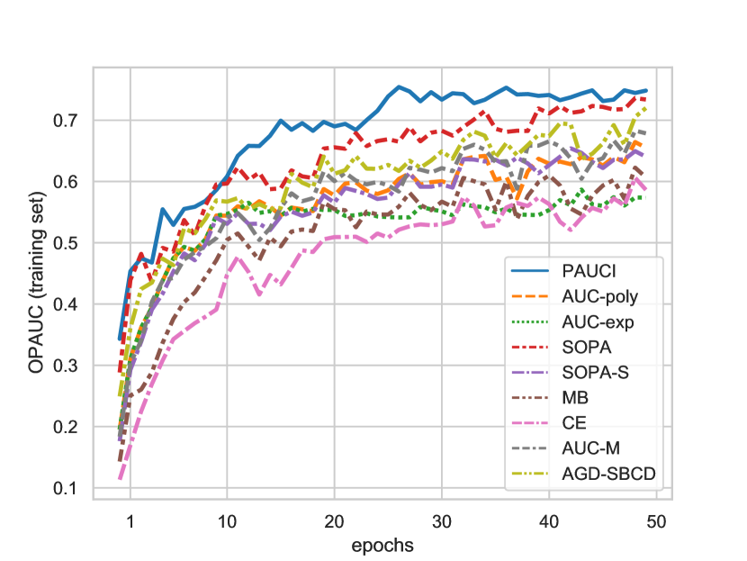
(a) CIFAR-10-LT-1

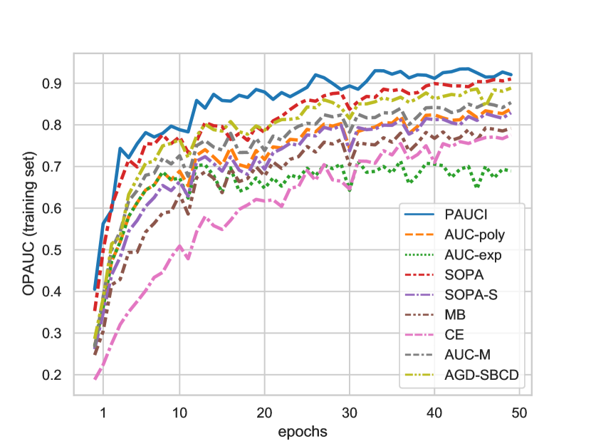
(b) CIFAR-10-LT-2

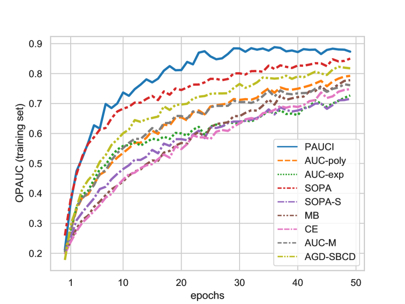
(c) CIFAR-10-LT-3

Figure 4: Convergence of OPAUC optimization.

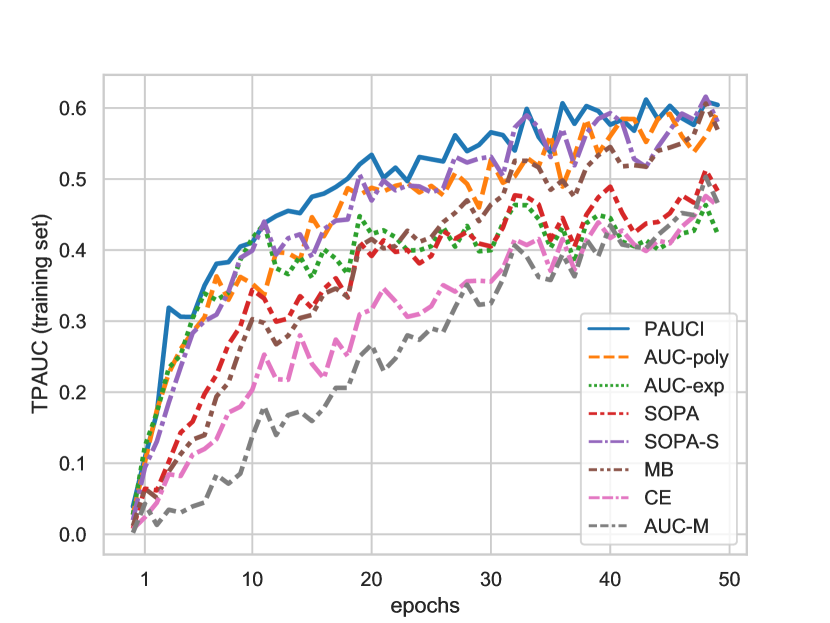
(a) CIFAR-10-LT-1

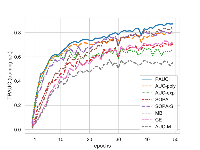
(b) CIFAR-10-LT-2

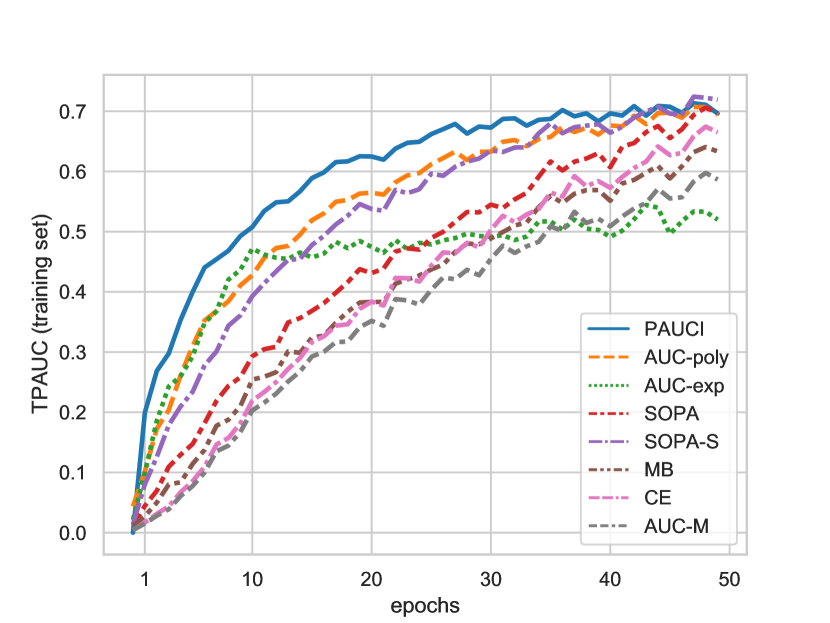
(c) CIFAR-10-LT-3

Figure 5: Convergence of TPAUC optimization.

In the convergence experiments, for sake of fairness, we did not use warm-up. All algorithms use hyperparameters in the performance experiments. We show the plots of training convergence in Fig.4 and Fig.5 on CIFAR-10 for both $\mathrm{OPAUC}$ and $\mathrm{TPAUC}$. Due to the space limitation, the other results could be found in Appendix.E. According to the figures, we can make the following observations: (1) Our algorithm and SOPA converge faster than other methods for $\mathrm{OPAUC}$. However, for $\mathrm{TPAUC}$ optimization, the SOPA converges very slowly due to its complicated algorithm, while our method still shows the best convergence property in most cases. (2) It’s notable that our algorithm converges to stabilize after twenty epochs in most cases. That means our method has better stability in practice.

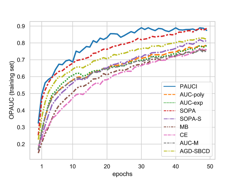
(a) CIFAR-100-Long-Tail-1

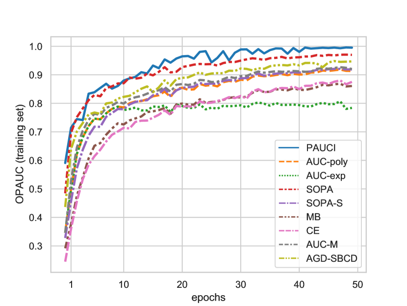
(b) CIFAR-100-Long-Tail-2

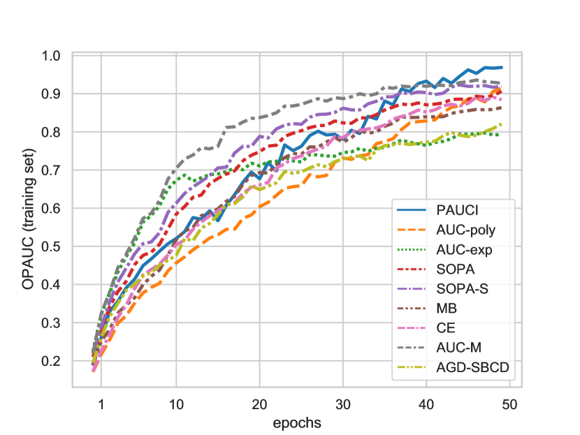
(c) CIFAR-100-Long-Tail-3

Figure 2: Convergence of OPAUC optimization.

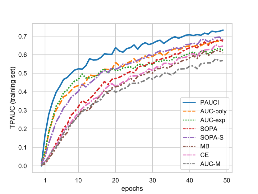
(d) CIFAR-100-Long-Tail-1

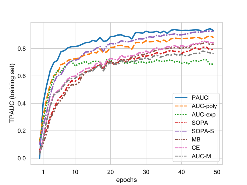
(e) CIFAR-100-Long-Tail-2

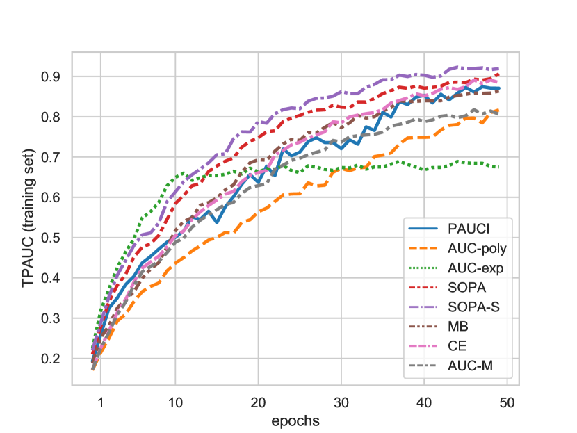
(f) CIFAR-100-Long-Tail-3

Figure 3: Convergence of TPAUC optimization.

7 Conclusion

In this paper, we focus on designing an efficient and asymptotically unbiased algorithm for PAUC. We propose a nonconvex strongly concave minimax instance-wise formulation for $\mathrm{OPAUC}$ and $\mathrm{TPAUC}$. In this way, we incorporate the instances selection into the loss calculation to eliminate the score ranking challenge. For $\mathrm{OPAUC}$ and $\mathrm{TPAUC}$, we employ an efficient stochastic minimax algorithm that ensures we can find a $\epsilon$-first order saddle point after $O(\epsilon^{-3})$ iterations. Moreover, we present a theoretical analysis of the generalization error of our formulation. Our conclusion may contribute to future work about AUC generalization. Finally, empirical studies over a range of long-tailed benchmark datasets speak to the effectiveness of our proposed algorithm.

8 Acknowledgements

This work was supported in part by the National Key R&D Program of China under Grant 2018AAA0102000, in part by National Natural Science Foundation of China: U21B2038, 61931008, 61836002, 6212200758 and 61976202, in part by the Fundamental Research Funds for the Central Universities, in part by Youth Innovation Promotion Association CAS, in part by the Strategic Priority Research Program of Chinese Academy of Sciences, Grant No. XDB28000000, in part by the National Postdoctoral Program for Innovative Talents under Grant BX2021298, and in part by mindspore, which is a new AI computing framework .

Checklist

1. For all authors…

   1. Do the main claims made in the abstract and introduction accurately reflect the paper’s contributions and scope? [Yes]

   2. Did you describe the limitations of your work? [N/A]

   3. Did you discuss any potential negative societal impacts of your work? [No] We have not discovered any negative societal impacts in our study.

   4. Have you read the ethics review guidelines and ensured that your paper conforms to them? [Yes]

2. If you are including theoretical results…

   1. Did you state the full set of assumptions of all theoretical results? [Yes]

   2. Did you include complete proofs of all theoretical results? [Yes]

3. If you ran experiments…

   1. Did you include the code, data, and instructions needed to reproduce the main experimental results (either in the supplemental material or as a URL)? [Yes]

   2. Did you specify all the training details (e.g., data splits, hyperparameters, how they were chosen)? [Yes]

   3. Did you report error bars (e.g., with respect to the random seed after running experiments multiple times)? [No] Our experiments are very time consuming.

   4. Did you include the total amount of compute and the type of resources used (e.g., type of GPUs, internal cluster, or cloud provider)? [Yes]

4. If you are using existing assets (e.g., code, data, models) or curating/releasing new assets…

   1. If your work uses existing assets, did you cite the creators? [Yes]

   2. Did you mention the license of the assets? [Yes]

   3. Did you include any new assets either in the supplemental material or as a URL? [Yes]

   4. Did you discuss whether and how consent was obtained from people whose data you’re using/curating? [No] Because we use the open source software and data.

   5. Did you discuss whether the data you are using/curating contains personally identifiable information or offensive content? [N/A]

5. If you used crowdsourcing or conducted research with human subjects…

   1. Did you include the full text of instructions given to participants and screenshots, if applicable? [N/A]

   2. Did you describe any potential participant risks, with links to Institutional Review Board (IRB) approvals, if applicable? [N/A]

   3. Did you include the estimated hourly wage paid to participants and the total amount spent on participant compensation? [N/A]

section

List of Appendix [sections] [sections]1

Appendix A Related work

Deep AUC Optimization. In the past few decades, AUC optimization has already achieved remarkable success in the long-tailed/imbalanced learning task [38]. A partial list of the related literature includes [13, 5, 35, 17, 27, 10, 29, 41]. In recent age, many studies focused on AUC optimization with stochastic gradient method. For example, on top of the square surrogate loss, [41] first proposed a minimax reformulation of the AUC. With a strongly convex regularizer, [26] improved the convergence rate of the stochastic learning algorithm for AUC to $O(1/T)$. In succession, [21, 14, 42] proposed some AUC optimization methods that can be applied to nonconvex deep neural networks.

Partial AUC (PAUC) Optimization. [22] first introduced the concept of PAUC. Earlier studies related to PAUC only paid attention to the simplest linear models. In [27], the PAUC is first optimized by a distribution-free rank-based method. [34] developed a non-parametric estimate of the PAUC, and selected features at each step to build the final classifier. [24] develops a cutting plane algorithm to find the most violated constraint instance, decomposing PAUC optimization into subproblems and solving them by an efficient structural SVM-based approach. However, most of the above approaches often fall into the non-differentiable property or intractable optimization problems, posing a significant obstacle to the end-to-end implementation. Using the Implicit Function Theorem, [20] formulated a rate-constrained optimization problem that modeled the quantile threshold as the output of a function of model parameters. As a milestone study, [39] simplifies the challenging sample-selected problem involved in PAUC optimization in a bi-level manner and thus facilitates the end-to-end optimization for PAUC of deep learning. Concretely, the inner-level optimization achieves instances selection, and the outer-level optimization minimizes the loss. However, their estimation may suffer from an approximation error with true PAUC. [44, 40] proposed a smooth estimator of PAUC and provided a sound theoretical convergence guarantee of their algorithm. Nevertheless, their algorithm is limited by a slow convergence rate, especially for TPAUC.

Generalization Analysis for Partial AUC Optimization. [25] presented the first generalization analysis for $\mathrm{OPAUC}$ and derived a uniform convergence generalization bound. Following their work, a recent study [39] extended this generalization bound to $\mathrm{TPAUC}$. However, limited by the pair-wise form of AUC, all of above studies require complicated decomposition. Moreover, their generalization analysis only hold for hard-threshold functions and VC-dimension. Based on our instance-wise reformulation, we show that the generalization of partial AUC is as simple as other instance-wise algorithm and can deal with real-valued score functions by Rademacher complexity.

Appendix B Convergence of the Bias without Regularization

Take $\mathrm{OPAUC}$ as an example, we will prove that the approximation induced by $r_{k}$ has a finite convergence rate which vanishes when $\kappa\rightarrow\infty$. For the sake of convenience, we denote the bias as:

$$\Delta_{\kappa}=\min_{f,(a,b)\in[0,1]^{2}}\max_{\gamma\in\Omega_{\gamma}}\min_{s^{\prime}\in\Omega_{s^{\prime}}}\underset{\bm{z}\sim S}{\hat{\mathbb{E}}}\Big{[}G_{op}^{\kappa}\left(f,a,b,\gamma,\boldsymbol{z},s^{\prime}\right)\Big{]}$$

$$~{}~{}~{}~{}~{}~{}~{}~{}~{}~{}~{}~{}-\min_{f,(a,b)\in[0,1]^{2}}\max_{\gamma\in\Omega_{\gamma}}\min_{s^{\prime}\in\Omega_{s^{\prime}}}\underset{\bm{z}\sim S}{\hat{\mathbb{E}}}\Big{[}G_{op}(f,a,b,\gamma,\boldsymbol{z},s^{\prime})\Big{]}$$

Specifically, we can also prove the following convergence condition holds without the regularization term:

Theorem 5.

With the assumption that $f(\bm{x})\in[0,1],\forall\bm{x}$, we have the following convergence result:

$$\lim_{\kappa\rightarrow\infty}\bigg{|}\min_{f,(a,b)\in[0,1]^{2}}\max_{\gamma\in\Omega_{\gamma}}\min_{s^{\prime}\in\Omega_{s^{\prime}}}\underset{\bm{z}\sim S}{\hat{\mathbb{E}}}\Big{[}G_{op}^{\kappa}\left(f,a,b,\gamma,\boldsymbol{z},s^{\prime}\right)\Big{]}$$ (33)

$$~{}~{}~{}~{}~{}~{}~{}~{}~{}~{}~{}~{}-\min_{f,(a,b)\in[0,1]^{2}}\max_{\gamma\in\Omega_{\gamma}}\min_{s^{\prime}\in\Omega_{s^{\prime}}}\underset{\bm{z}\sim S}{\hat{\mathbb{E}}}\Big{[}G_{op}(f,a,b,\gamma,\boldsymbol{z},s^{\prime})\Big{]}\bigg{|}$$

$$=0.$$

Moreover, we can also obtain a convergence rate:

$$\Delta_{\kappa}=O(1/\kappa).$$ (34)

Proof.

Denote:

$$\Delta_{\kappa}= \bigg{|}\min_{f,(a,b)\in[0,1]^{2}}\max_{\gamma\in\Omega_{\gamma}}\min_{s^{\prime}\in\Omega_{s^{\prime}}}\underset{\bm{z}\sim S}{\hat{\mathbb{E}}}\Big{[}G_{op}^{\kappa}\left(f,a,b,\gamma,\boldsymbol{z},s^{\prime}\right)\Big{]}$$ (35)

$$~{}-\min_{f,(a,b)\in[0,1]^{2}}\max_{\gamma\in\Omega_{\gamma}}\min_{s^{\prime}\in\Omega_{s^{\prime}}}\underset{\bm{z}\sim S}{\hat{\mathbb{E}}}\Big{[}G_{op}(f,a,b,\gamma,\boldsymbol{z},s^{\prime})\Big{]}\bigg{|}.$$

First, we have:

$$\limsup_{\kappa\rightarrow+\infty}\Delta_{\kappa}\leq \underbrace{\limsup_{\kappa\rightarrow+\infty}\sup_{f,(a,b)\in[0,1]^{2},\gamma\in\Omega_{\gamma},s^{\prime}\in\Omega_{s^{\prime}},\boldsymbol{z}\sim\mathcal{D}_{\mathcal{Z}}}\left|\frac{\log(1+\exp(\kappa\cdot g))}{\kappa}-[g]_{+}\right|}_{(a)}.$$ (36)

where $g=(f(\bm{x})-b)^{2}+2(1+\gamma)f(\bm{x})-s^{\prime}$ and $[x]_{+}=\max\{x,0\}$. Since $g\in[-5,5]$ in the feasible set, we have:

$$(a)\leq\limsup_{\kappa\rightarrow+\infty}\sup_{x\in[-5,5]}\left|\frac{\log(1+\exp(\kappa\cdot x))}{\kappa}-[x]_{+}\right|.$$ (37)

Next we prove that

$$\underset{\kappa\to\infty}{\limsup}\underset{x\in[-5,5]}{\sup}\left[\left|\frac{\log(1+\exp(\kappa\cdot x))}{\kappa}-[x]_{+}\right|\right]\leq 0.$$ (38)

For the sake of simplicity, we denote:

$$\ell(x)=\left|\frac{\log(1+\exp(\kappa\cdot x))}{\kappa}-[x]_{+}\right|.$$ (39)

It is easy to see that, when $x<0$, we have:

$$\ell(x)^{\prime}=\left(\frac{\log(1+\exp(\kappa\cdot x))}{\kappa}\right)^{\prime}\geq 0.$$ (40)

When $x>0$, we have:

$$\ell(x)^{\prime}=\left(\frac{\log(1+\exp(\kappa\cdot x))}{\kappa}-x\right)^{\prime}\leq 0.$$ (41)

Hence, the supremum must be attained at $x=0$. We thus have:

$$(a)\leq\limsup_{\kappa\rightarrow+\infty}\frac{\log(2)}{\kappa}=0.$$ (42)

Obviously, the absolute value ensures that:

$$\liminf_{\kappa\rightarrow+\infty}\Delta_{\kappa}\geq 0.$$ (43)

The result follows from the fact:

$$0\leq\liminf_{\kappa\rightarrow+\infty}\Delta_{\kappa}\leq\limsup_{\kappa\rightarrow+\infty}\Delta_{\kappa}\leq 0.$$ (44)

Moreover, from the proof above, we also obtain a convergence rate:

$$\Delta_{\kappa}=O(1/\kappa).$$ (45)

∎

Appendix C The Constrained Reformulation

In this section, we will prove that the constrained reformulation which is used in the proof of Thm.2 and Thm.8. Our proof can be established by Lem.2, Lem.3, and Thm.6. Throughout the proof, we will define:

$$a^{*}=\mathbb{E}_{\bm{x}\sim\mathcal{D}_{\mathcal{P}}}[f(\bm{x})] :=E_{+}$$ (46)

$$b^{*}=\mathbb{E}_{\bm{x}^{\prime}\sim\mathcal{D}_{\mathcal{N}}}[f(\bm{x}^{\prime})|f(\bm{x}^{\prime})\geq\eta_{\beta}(f)] :=E_{-}$$

$$b^{*}-a^{*} :=\Delta E$$

$$\tilde{a}^{*}=\mathbb{E}_{\bm{x}\sim\mathcal{D}_{\mathcal{P}}}[f(\bm{x})|f(\bm{x})\leq\eta_{\alpha}(f)] :=\tilde{E}_{+}$$

$$b^{*}-\tilde{a}^{*} :=\Delta\tilde{E}$$

$$\mathbb{E}_{\bm{x}\sim\mathcal{D}_{\mathcal{P}}}[(f(\bm{x})-a)^{2}] :={E}_{a}$$

$$\mathbb{E}_{\bm{x}\sim\mathcal{D}_{\mathcal{P}}}[(f(\bm{x})-a)^{2}|f(\bm{x})\leq\eta_{\alpha}(f)] :=\tilde{E}_{a}$$

$$\mathbb{E}_{\bm{x}^{\prime}\sim\mathcal{D}_{\mathcal{N}}}[(f(\bm{x}^{\prime})-b)^{2}|f(\bm{x}^{\prime})\geq\eta_{\beta}(f)] :=E_{b}$$

$$\mathbb{E}_{\bm{x}\sim\mathcal{D}_{\mathcal{P}}}[f(\bm{x})^{2}|f(\bm{x})\leq\eta_{\alpha}(f)] :=E_{+,2}$$

$$\mathbb{E}_{\bm{x}^{\prime}\sim\mathcal{D}_{\mathcal{N}}}[f(\bm{x}^{\prime})^{2}|f(\bm{x}^{\prime})\geq\eta_{\beta}(f)] :=E_{-,2}$$

Lemma 2.

(The Reformulation for OPAUC) For a fixed scoring function $f$, the following two problems shares the same optimum, given that the scoring function satisfies: $f(\bm{x})\in[0,1],~{}\forall\bm{x}$:

$$\boldsymbol{(OP1)}\min_{(a,b)\in[0,1]^{2}}\max_{\gamma\in[-1,1]}\mathbb{E}_{\bm{x}\sim\mathcal{D}_{\mathcal{P}}}[(f(\bm{x})-a)^{2}]+\mathbb{E}_{\bm{x}^{\prime}\sim\mathcal{D}_{\mathcal{N}}}[(f(\bm{x}^{\prime})-b)^{2}|f(\bm{x}^{\prime})\geq\eta_{\beta}(f)]$$ (47)

$$+2\Delta E+2\gamma\Delta E-\gamma^{2}$$

$$\boldsymbol{(OP2)}\min_{(a,b)\in[0,1]^{2}}\max_{\gamma\in[b-1,1]}\mathbb{E}_{\bm{x}\sim\mathcal{D}_{\mathcal{P}}}[(f(\bm{x})-a)^{2}]+\mathbb{E}_{\bm{x}^{\prime}\sim\mathcal{D}_{\mathcal{N}}}[(f(\bm{x}^{\prime})-b)^{2}|f(\bm{x}^{\prime})\geq\eta_{\beta}(f)]$$

$$+2\Delta E+2\gamma\Delta E-\gamma^{2}$$

Remark 2.

$\boldsymbol{(OP1)}$ and $\boldsymbol{(OP2)}$ have the equivalent formulation:

$$\boldsymbol{(OP1)}\Leftrightarrow\min_{(a,b)\in[0,1]^{2}} \max_{\gamma\in[-1,1]}\mathbb{E}_{\bm{z}\sim\mathcal{D}_{\mathcal{Z}}}\Big{[}\Large[(f(\bm{x})-a)^{2}-2(1+\gamma)f(\bm{x})\Large]y/p-\gamma^{2}$$ (48)

$$\Large[(f(\bm{x})-b)^{2}+2(1+\gamma)f(\bm{x})\Large]\cdot[(1-y)\mathbb{I}_{f(\bm{x})\geq\eta_{\beta}(f)}]/[(1-p)\beta]\big{]}.$$

$$\boldsymbol{(OP2)}\Leftrightarrow\min_{(a,b)\in[0,1]^{2}} \max_{\gamma\in[b-1,1]}\mathbb{E}_{\bm{z}\sim\mathcal{D}_{\mathcal{Z}}}\Big{[}\Large[(f(\bm{x})-a)^{2}-2(1+\gamma)f(\bm{x})\Large]y/p-\gamma^{2}$$ (49)

$$\Large[(f(\bm{x})-b)^{2}+2(1+\gamma)f(\bm{x})\Large]\cdot[(1-y)\mathbb{I}_{f(\bm{x})\geq\eta_{\beta}(f)}]/[(1-p)\beta]\big{]}.$$

Proof.

From the proof of our main paper, we know that $(OP1)$ has a closed-form minimum:

$$E_{a^{*}}+{E}_{b^{*}}+(\Delta E)^{2}+2\Delta E.$$ (50)

Hence, we only need to prove that $(OP2)$ has the same minimum solution. By expanding $(OP2)$, we have:

$$\min_{(a,b)\in[0,1]^{2}}\max_{\gamma\in[b-1,1]}\mathbb{E}_{\bm{z}\sim\mathcal{D}_{\mathcal{Z}}}[F_{op}(f,a,b,\gamma,\eta_{\beta}(f),\bm{z})] =$$ (51)

$$2\Delta E+\min_{a\in[0,1]}E_{a}+\min_{b\in[0,1]}\max_{\gamma\in[b-1,1]}F_{0}$$

where

$$F_{0}:=E_{b}+2\gamma\Delta E-\gamma^{2}$$ (52)

Obviously since $a$ is decoupled with $b,\gamma$, we have:

$$\min_{a\in[0,1]}E_{a}=E_{a^{*}}$$ (53)

Now, we solve the minimax problem of $F_{0}$. For any fixed feasible $b$, the inner max problem is a truncated quadratic programming, which has a unique and closed-form solution. Hence, we first solve the inner maximization problem for fixed $b$, and then represent the minimax problem as a minimization problem for $b$. Specifically, we have:

$$\left(\max_{\gamma\in[b-1,1]}2\gamma\Delta E-\gamma^{2}\right)=\begin{cases}(\Delta E)^{2},&\Delta E\geq b-1\\ 2(b-1)\Delta E-(b-1)^{2},&\text{otherwise}\end{cases}$$ (54)

Thus, we have:

$$\min_{b\in[0,1]}\max_{\gamma\in[b-1,1]}F_{0}=\min_{b\in[0,1]}F_{1}$$ (55)

where

$$F_{1}=\begin{cases}&F_{1,0}(b):=E_{b}+(\Delta E)^{2},b-1\leq\Delta E\\ &F_{1,1}(b):=E_{-,2}-2bE_{-}+2b-1+2(b-1)\Delta E,\text{otherwise}\end{cases}$$ (56)

It is easy to see that both cases of $F_{1}$ are convex functions w.r.t $b$. So, we can find the global minimum by comparing the minimum of $F_{1,0}$ and $F_{1,1}$.

• CASE 1: $\Delta E\geq b-1$. It is easy to see that $b^{*}=E_{-}\in(-\infty,1+\Delta E]$, by taking the derivative to zero, we have, the optimum value is obtained at $b=E_{-}$ for $F_{1,0}$.

• CASE 2: $\Delta E\leq b-1$. Again by taking the derivative, we have:

  $$F_{1,1}(b)^{\prime}=-2E_{-}+2+2\Delta E=2-2E_{+}\geq 0$$ (57)

  We must have:

  $$\inf_{b\geq 1+\Delta E}F_{1,1}(b)~{}\geq~{}F_{1,1}(1+\Delta E)~{}=~{}F_{1,0}(1+\Delta E)~{}\geq~{}F_{1,0}(E_{-})~{}=~{}F_{1,0}(b^{*})$$ (58)

• Putting all together Hence the global minimum of $F_{1}$ is obtained at $b^{*}$ with:

  $$F_{1}(b^{*})=F_{1,0}(b^{*})=E_{b^{*}}+(\Delta E)^{2}$$ (59)

Hence, we have $(OP2)$ has the minimum value:

$$E_{a^{*}}+E_{b^{*}}+(\Delta E)^{2}+2\Delta E$$ (60)

∎

Now, we use a similar trick to prove the result for TPAUC:

Lemma 3.

(The Reformulation for TPAUC) For a fixed scoring function $f$, the following two problems shares the same optimum, given that the scoring function satisfies: $f(\bm{x})\in[0,1],~{}\forall\bm{x}$:

$$\boldsymbol{(OP3)}\min_{f,(a,b)\in[0,1]^{2}}\max_{\gamma\in[-1,1]} \mathbb{E}_{\bm{x}\sim\mathcal{D}_{\mathcal{P}}}[(f(\bm{x})-a)^{2}|f(\bm{x})\leq\eta_{\alpha}(f)]$$ (61)

$$+ \mathbb{E}_{\bm{x}^{\prime}\sim\mathcal{D}_{\mathcal{N}}}[(f(\bm{x}^{\prime})-b)^{2}|f(\bm{x}^{\prime})\geq\eta_{\beta}(f)]$$

$$+ 2\Delta\tilde{E}+2\gamma\Delta\tilde{E}-\gamma^{2}.$$

$$\boldsymbol{(OP4)}\min_{f,(a,b)\in[0,1]^{2}}\max_{\gamma\in[\max\{-a,b-1\},1]} \mathbb{E}_{\bm{x}\sim\mathcal{D}_{\mathcal{P}}}[(f(\bm{x})-a)^{2}|f(\bm{x})\leq\eta_{\alpha}(f)]$$

$$+ \mathbb{E}_{\bm{x}^{\prime}\sim\mathcal{D}_{\mathcal{N}}}[(f(\bm{x}^{\prime})-b)^{2}|f(\bm{x}^{\prime})\geq\eta_{\beta}(f)]$$

$$+ 2\Delta\tilde{E}+2\gamma\Delta\tilde{E}-\gamma^{2}.$$

Remark 3.

$\boldsymbol{(OP3)}$ and $\boldsymbol{(OP4)}$ have the equivalent formulation:

$$\boldsymbol{(OP3)}\Leftrightarrow\min_{(a,b)\in[0,1]^{2}} \max_{\gamma\in[-1,1]}\mathbb{E}_{\bm{z}\sim\mathcal{D}_{\mathcal{Z}}}\Big{[}\Large[(f(\bm{x})-a)^{2}-2(1+\gamma)f(\bm{x})\Large]\cdot[y\mathbb{I}_{f(\bm{x})\leq\eta_{\alpha}(f)}]/p-\gamma^{2}$$ (62)

$$\Large[(f(\bm{x})-b)^{2}+2(1+\gamma)f(\bm{x})\Large]\cdot[(1-y)\mathbb{I}_{f(\bm{x})\geq\eta_{\beta}(f)}]/[(1-p)\beta]\Big{]}.$$

$$\boldsymbol{(OP4)}\Leftrightarrow\min_{(a,b)\in[0,1]^{2}} \max_{\gamma\in[\max\{-a,b-1\}1]}\mathbb{E}_{\bm{z}\sim\mathcal{D}_{\mathcal{Z}}}\Big{[}\Large[(f(\bm{x})-a)^{2}-2(1+\gamma)f(\bm{x})\Large]\cdot[y\mathbb{I}_{f(\bm{x})\leq\eta_{\alpha}(f)}]/p$$ (63)

$$\Large[(f(\bm{x})-b)^{2}+2(1+\gamma)f(\bm{x})\Large]\cdot[(1-y)\mathbb{I}_{f(\bm{x})\geq\eta_{\beta}(f)}]/[(1-p)\beta]-\gamma^{2}\Big{]}.$$

Proof.

Again, $(OP3)$ has the minimum value:

$$\tilde{E}_{\tilde{a}^{*}}+E_{b^{*}}+(\Delta\tilde{E})^{2}+2\Delta\tilde{E}$$ (64)

We proof that $(OP4)$ ends up with the minimum value. By expanding $(OP4)$, we have:

$$(OP4)=2\Delta\tilde{E}+\min_{(a,b)\in[0,1]^{2}}\max_{\gamma\in[\max\{-a,b-1\},1]}F_{3}$$ (65)

where

$$F_{3}:=\tilde{E}_{a}+E_{b}+2\Delta\tilde{E}+2\gamma\Delta\tilde{E}-\gamma^{2}$$ (66)

For any fixed feasible $a,b$, the inner max problem is a truncated quadratic programming, which has a unique and closed-form solution. Specifically, define $c=\max\{-a,b-1\}$, we have:

$$\left(\max_{\gamma\in[c,1]}2\gamma\Delta\tilde{E}-\gamma^{2}\right)=\begin{cases}(\Delta\tilde{E})^{2},&\Delta\tilde{E}\geq c\\ 2c\Delta\tilde{E}-c^{2},&\text{otherwise}\end{cases}$$ (67)

Thus, we have:

$$\min_{(a,b)\in[0,1]^{2}}\max_{\gamma\in[c,1]}F_{3}=\min_{(a,b)\in[0,1]}F_{4}$$ (68)

where

$$F_{4}=\begin{cases}&F_{4,0}(a,b):=\tilde{E}_{a}+E_{b}+(\Delta\tilde{E})^{2},c\leq\Delta\tilde{E}\\ &F_{4,1}(a,b):=\tilde{E}_{a}+E_{-,2}-2bE_{-}+2(b-1)\Delta\tilde{E}+2b-1,b-1\geq\Delta\tilde{E},-a\leq b-1\\ &F_{4,2}(a,b):=E_{b}+E_{+,2}-2a\tilde{E}_{+}-2a\Delta\tilde{E},-a\geq\Delta\tilde{E},b-1\leq-a\end{cases}$$ (69)

It is easy to see that both cases of $F_{1}$ are convex functions w.r.t $b$. So, we can find the global minimum by comparing the minimum of $F_{1,0}$ and $F_{1,1}$.

• CASE 1: $\Delta\tilde{E}\geq\max\{-a,b-1\}$.

  It is easy to check that when $a=\tilde{E}_{+},b=E_{-}$, we have $-a\leq\Delta\tilde{E}$ and $b-1\leq\Delta\tilde{E}$. It is easy to see that $a,b$ are decoupled in the expression of $F_{4,0}(a,b)$. By setting:

  $$\frac{\partial F_{4,0}(a,b)}{\partial a}=0,$$ (70)

  $$\frac{\partial F_{4,0}(a,b)}{\partial b}=0$$

  We know that the minimum solution is attained at $a=\tilde{a}^{*}$, $b=b^{*}$. Then the minimum value of $F_{4,0}(a,b)$ at this range becomes:

  $$\tilde{E}_{\tilde{a}^{*}}+E_{b^{*}}+(\Delta\tilde{E})^{2}$$ (71)

  Moreover, we will also use the fact that $E_{\tilde{a}^{*}}$ and $E_{b^{*}}$ are also the global minimum for $E_{a}$ and $E_{b}$, respectively.

• CASE 2: $b-1\geq\Delta\tilde{E},~{}-a\leq b-1$.

  It is easy to see that $E_{a}\geq E_{\tilde{a}^{*}}$ in this case. According to the same derivation as in Lem.2 CASE 2, we have:

  $$E_{-,2}-2bE_{-}+2(b-1)\Delta\tilde{E}+2b-1\geq E_{b^{*}}+(\Delta\tilde{E})^{2}$$ (72)

  holds when $b-1\geq\Delta\tilde{E}$. Recall that CASE 2 is include in the condition $b-1\geq\Delta\tilde{E}$. So, under the condition of CASE 2:

  $$F_{4,1}(a,b)\geq\tilde{E}_{\tilde{a}^{*}}+E_{b^{*}}+(\Delta\tilde{E})^{2}$$ (73)

• CASE 3: $-a\geq\Delta\tilde{E},b-1\leq-a$

  In this case, we have $E_{b}\geq E_{b^{*}}$. It remains to check:

  $$g(a)=-2a\tilde{E}_{+}-2a\Delta\tilde{E}$$ (74)

  By taking derivative, we have:

  $$g^{\prime}(a)=-2\tilde{E}_{+}-2\Delta\tilde{E}=-2\tilde{E}_{-}\leq 0.$$ (75)

  Similar as the proof of CASE 2, when $-a\geq\Delta\tilde{E}$, we have:

  $$g(a)\geq\tilde{E}_{\tilde{a}^{*}}+(\Delta\tilde{E})^{2}$$ (76)

  and thus

  $$F_{4,2}(a,b)\geq\tilde{E}_{\tilde{a}^{*}}+E_{b^{*}}+(\Delta\tilde{E})^{2}$$ (77)

  holds. Since the condition of CASE 3 is included in the set $-a\geq\Delta\tilde{E}$:

  $$F_{4,2}(a,b)\geq\tilde{E}_{\tilde{a}^{*}}+E_{b^{*}}+(\Delta\tilde{E})^{2}$$ (78)

  holds under the condition of CASE 3.

• Putting altogether: The minimum value of $(OP4)$ reads:

  $$\tilde{E}_{\tilde{a}^{*}}+E_{b^{*}}+(\Delta\tilde{E})^{2}+2\Delta\tilde{E}$$ (79)

  which is the same as $(OP3)$.

∎

Finally, since for each fixed $f$ $(OP3)=(OP4)$, and $(OP1)=(OP2)$ . We can then claim the following theorem:

Theorem 6.

(Constrainted Reformulation)

$$\min_{f}(OP1)=\min_{f}(OP2),~{}~{}\min_{f}(OP3)=\min_{f}(OP4)$$ (80)

Remark 4.

Since the calculation is irelevant to the definition of the expectation, the replace the population-level expectation with the empirical expectation over the training data.

Remark 5.

By applying Theorem 1, we can get the reformulation result in Theorem 2

for $\mathrm{OPAUC}$

$$\min_{f,(a,b)\in[0,1]^{2}}\max_{\gamma\in[b-1,1]}\min_{s^{\prime}\in\Omega_{s^{\prime}}}\mathbb{E}_{\bm{z}\sim\mathcal{D}_{\mathcal{Z}}}[G_{op}(f,a,b,\gamma,\bm{z},s^{\prime})]$$ (81)

where

$$G_{op}(f,a,b,\gamma,\bm{z},s^{\prime}) =[(f(\bm{x})-a)^{2}-2(1+\gamma)f(\bm{x})]y/p-\gamma^{2}$$ (82)

$$+\left(\beta s^{\prime}+\left[(f(\bm{x})-b)^{2}+2(1+\gamma)f(\bm{x})-s^{\prime}\right]_{+}\right)(1-y)/[\beta(1-p)].$$

for $\mathrm{TPAUC}$

$$\min_{f,(a,b)\in[0,1]^{2}}\max_{\gamma\in[\max\{-a,b-1\},1]}\min_{s\in\Omega_{s},s^{\prime}\in\Omega_{s^{\prime}}}\mathbb{E}_{\bm{z}\sim\mathcal{D}_{\mathcal{Z}}}[G_{tp}(f,a,b,\gamma,\bm{z},s,s^{\prime})]$$ (83)

where

$$G_{tp}(f,a,b,\gamma,\bm{z},s,s^{\prime}) =\left(\alpha s+r_{\kappa}\left((f(\bm{x})-a)^{2}-2(1+\gamma)f(\bm{x})-s\right)\right)y/(\alpha p)-\gamma^{2}$$ (84)

$$+\left(\beta s^{\prime}+r_{\kappa}\left((f(\bm{x})-b)^{2}+2(1+\gamma)f(\bm{x})-s^{\prime}\right)\right)(1-y)/[\beta(1-p)].$$

Appendix D Reformulation for TPAUC

According to Eq.(5), given a surrogate loss $\ell$ and the finite dataset $S$, maximizing $\mathrm{TPAUC}$ and $\hat{\mathrm{AUC}}_{\alpha,\beta}(f,S)$ is equivalent to solving the following problems, respectively:

$$\underset{f}{\min}~{}\mathcal{R}_{\alpha,\beta}(f)=\mathbb{E}_{\bm{x}\sim\mathcal{D}_{\mathcal{P}},\bm{x}^{\prime}\sim\mathcal{D}_{\mathcal{N}}}\left[\mathbb{I}_{f(\bm{x})\leq\eta_{\alpha}(f)}\cdot\mathbb{I}_{f(\bm{x}^{\prime})\geq\eta_{\beta}(f)}\cdot\ell(f(\bm{x})-f(\bm{x}^{\prime}))\right],$$ (85)

$$\underset{f}{\min}\ \hat{\mathcal{R}}_{\alpha,\beta}(f,S)=\sum_{i=1}^{n_{+}^{\alpha}}\sum_{j=1}^{n_{-}^{\beta}}\frac{\ell{\left(f(\bm{x}_{[i]})-f(\bm{x}^{\prime}_{[j]})\right)}}{n_{+}^{\alpha}n_{-}^{\beta}}.$$ (86)

Similar to $\mathrm{OPAUC}$, we have the following theorem shows an instance-wise reformulation of the $\mathrm{TPAUC}$ optimization problem:

Theorem 7.

Assuming that $f(\bm{x})\in[0,1]$, $\forall\bm{x}\in\mathcal{X}$, $F_{tp}(f,a,b,\gamma,t,t^{\prime},\bm{z})$ is defined as:

$$F_{tp}( f,a,b,\gamma,t,t^{\prime},\bm{z})=(f(\bm{x})-a)^{2}y\mathbb{I}_{f(\bm{x})\leq t}/(\alpha p)+(f(\bm{x})-b)^{2}(1-y)\mathbb{I}_{f(\bm{x}^{\prime})\geq t^{\prime}}/[\beta(1-p)]$$ (87)

$$+2(1+\gamma)f(\bm{x})(1-y)\mathbb{I}_{f(\bm{x}^{\prime})\geq t^{\prime}}/[\beta(1-p)]-2(1+\gamma)f(\bm{x})y/p\mathbb{I}_{f(\bm{x})\leq t}/(\alpha p)-\gamma^{2},$$

where $y=1$ for positive instances, $y=0$ for negative instances and we have the following conclusions:

1. (Population Version.) We have:

   $$\underset{f}{\min}\ {\mathcal{R}}_{\alpha,\beta}(f)\Leftrightarrow\underset{f,(a,b)\in[0,1]^{2}}{\min}\ \underset{\gamma\in[-1,1]}{\max}\ {\color[rgb]{0,0,1}\underset{\bm{z}\sim\mathcal{D}_{\mathcal{Z}}}{\mathbb{E}}}\left[F_{tp}(f,a,b,\gamma,{\color[rgb]{0,0,1}\eta_{\alpha}(f)},{\color[rgb]{0,0,1}\eta_{\beta}(f)},\bm{z})\right],$$ (88)

   where ${\color[rgb]{0,0,1}\eta_{\alpha}(f)}=\arg\min_{{\color[rgb]{0,0,1}\eta_{\alpha}}\in\mathbb{R}}\left[\mathbb{E}_{\bm{x}\sim\mathcal{D}_{\mathcal{P}}}[\mathbb{I}_{f(\bm{x})\leq\ {\color[rgb]{0,0,1}\eta_{\alpha}}}]=\alpha\right]$ and ${\color[rgb]{0,0,1}\eta_{\beta}(f)}=\arg\min_{{\color[rgb]{0,0,1}\eta_{\beta}}\in\mathbb{R}}\left[\mathbb{E}_{\bm{x}^{\prime}\sim\mathcal{D}_{\mathcal{N}}}[\mathbb{I}_{f(\bm{x}^{\prime})\geq\ {\color[rgb]{0,0,1}\eta_{\beta}}}]=\beta\right]$.

2. (Empirical Version.) Moreover, given a training dataset $S$ with sample size $n$, denote:

   $${\color[rgb]{0.76,0.01,0}\hat{\mathbb{E}}_{z\sim S}}[F_{tp}(f,a,b,\gamma,{\color[rgb]{0.76,0.01,0}\hat{\eta}_{\alpha}(f)},{\color[rgb]{0.76,0.01,0}\hat{\eta}_{\beta}(f)},\bm{z})]=\frac{1}{n}\sum_{i=1}^{n}F_{tp}(f,a,b,\gamma,{\color[rgb]{0.76,0.01,0}\hat{\eta}_{\alpha}(f)},{{\color[rgb]{0.76,0.01,0}\hat{\eta}_{\beta}(f)}},\bm{z}),$$

   where ${\color[rgb]{0.76,0.01,0}\hat{\eta}_{\alpha}(f)}$ and ${\color[rgb]{0.76,0.01,0}\hat{\eta}_{\beta}(f)}$ are the empirical quantile of the positive and negative instances in $S$, respectively. We have:

   $$\underset{f}{\min}\ \hat{\mathcal{R}}_{\alpha,\beta}(f,S)\Leftrightarrow\underset{f,(a,b)\in[0,1]^{2}}{\min}\ \underset{\gamma\in[-1,1]}{\max}\ {\color[rgb]{0.76,0.01,0}\underset{\bm{z}\sim S}{\hat{\mathbb{E}}}}\left[F_{tp}(f,a,b,\gamma,{\color[rgb]{0.76,0.01,0}\hat{\eta}_{\alpha}(f)},{\color[rgb]{0.76,0.01,0}\hat{\eta}_{\beta}(f)},\bm{z})\right],$$ (89)

Thm.7 provides a support to convert the pair-wise loss into instance-wise loss for $\mathrm{TPAUC}$. Actually, for $\mathcal{R}_{\alpha,\beta}(f)$, we can just reformulate it as an Average Top-$k$ (ATk) loss. Denote $\ell_{+}(\bm{x})=(f(\bm{x})-a)^{2}-2(1+\gamma)f(\bm{x})$ and $\ell_{-}(\bm{x}^{\prime})=(f(\bm{x}^{\prime})-b)^{2}+2(1+\gamma)f(\bm{x}^{\prime})$. In the proof of the next theorem, we will show that $\ell_{+}(\bm{x})$ is an decreasing function and $\ell_{-}(\bm{x}^{\prime})$ is an increasing function w.r.t. $f(\bm{x})$ and $f(\bm{x}^{\prime})$, namely:

$$\mathbb{E}_{\bm{x}\sim\mathcal{D}_{\mathcal{P}}}[\mathbb{I}_{f(\bm{x})\leq\eta_{\alpha}(f)}\cdot\ell_{+}(\bm{x})]=\min_{s}\frac{1}{\alpha}\cdot\mathbb{E}_{\bm{x}\sim\mathcal{D}_{\mathcal{P}}}[\alpha s+[\ell_{+}(\bm{x})-s]_{+}],$$ (90)

$$\mathbb{E}_{\bm{x}^{\prime}\sim\mathcal{D}_{\mathcal{N}}}[\mathbb{I}_{f(\bm{x}^{\prime})\geq\eta_{\beta}(f)}\cdot\ell_{-}(\bm{x}^{\prime})]=\min_{s^{\prime}}\frac{1}{\beta}\cdot\mathbb{E}_{\bm{x}^{\prime}\sim\mathcal{D}_{\mathcal{N}}}[\beta s^{\prime}+[\ell_{-}(\bm{x}^{\prime})-s^{\prime}]_{+}],$$ (91)

The similar result holds for $\hat{\mathcal{R}}_{\alpha,\beta}(f,S)$. Then, we can reach to Thm.8

Theorem 8.

Assuming that $f(\bm{x})\in[0,1]$, for all $\bm{x}\in\mathcal{X}$, we have the equivalent optimization for $\mathrm{TPAUC}$:

$$\underset{f,(a,b)\in[0,1]^{2}}{\min}\ \underset{\gamma\in[-1,1]}{\max}\ {\color[rgb]{0,0,1}\underset{\bm{z}\sim\mathcal{D}_{\mathcal{Z}}}{\mathbb{E}}}[F_{tp}(f,a,b,\gamma,{\color[rgb]{0,0,1}\eta_{\alpha}(f)},{\color[rgb]{0,0,1}\eta_{\beta}(f)},\bm{z})]$$ (92)

$$\Leftrightarrow\underset{f,(a,b)\in[0,1]^{2}}{\min}\ \underset{\gamma\in\Omega_{\gamma}}{\max}\ \underset{s\in\Omega_{s},s^{\prime}\in\Omega_{s^{\prime}}}{\min}\ {\color[rgb]{0,0,1}\underset{\bm{z}\sim\mathcal{D}_{\mathcal{Z}}}{\mathbb{E}}}[G_{tp}(f,a,b,\gamma,\bm{z},s,s^{\prime})],$$

$$\underset{f,(a,b)\in[0,1]^{2}}{\min}\ \underset{\gamma\in\Omega_{\gamma}}{\max}\ {\color[rgb]{0.76,0.01,0}\underset{\bm{z}\sim S}{\hat{\mathbb{E}}}}[F_{tp}(f,a,b,\gamma,{\color[rgb]{0.76,0.01,0}\hat{\eta}_{\alpha}(f)},{\color[rgb]{0.76,0.01,0}\hat{\eta}_{\beta}(f)},\bm{z})]$$ (93)

$$\Leftrightarrow\underset{f,(a,b)\in[0,1]^{2}}{\min}\ \underset{\gamma\in\Omega_{\gamma}}{\max}\ \underset{s\in\Omega_{s},s^{\prime}\in\Omega_{s^{\prime}}}{\min}\ {\color[rgb]{0.76,0.01,0}\underset{\bm{z}\sim S}{\hat{\mathbb{E}}}}[G_{tp}(f,a,b,\gamma,\bm{z},s,s^{\prime})],$$

where $\Omega_{\gamma}=[\max\{b-1,-a\},1]$, $\Omega_{s}=[-4,1]$, $\Omega_{s^{\prime}}=[0,5]$ and

$$G_{tp}(f,a,b,\gamma, \bm{z},s,s^{\prime})=\left(\alpha s+\left[(f(\bm{x})-a)^{2}-2(1+\gamma)f(\bm{x})-s\right]_{+}\right)y/(\alpha p)$$ (94)

$$+\left(\beta s^{\prime}+\left[(f(\bm{x})-b)^{2}+2(1+\gamma)f(\bm{x})-s^{\prime}\right]_{+}\right)(1-y)/[\beta(1-p)]-\gamma^{2}.$$

Similar to $\mathrm{OPAUC}$, we can get a regularized non-convex strongly-concave $\mathrm{TPAUC}$ optimization problem:

$$\underset{f,(a,b)\in[0,1]^{2}}{\min}\ \underset{\gamma\in\Omega_{\gamma}}{\max}\min_{s\in\Omega_{s},s^{\prime}\in\Omega_{s^{\prime}}}\ {\color[rgb]{0,0,1}\underset{\bm{z}\sim\mathcal{D}_{\mathcal{Z}}}{\mathbb{E}}}[G_{tp}^{{{\color[rgb]{0,0,1}\kappa}},{\color[rgb]{0.76,0.01,0}\omega}}]\Leftrightarrow\underset{f,(a,b)\in[0,1]^{2},s\in\Omega_{s},s^{\prime}\in\Omega_{s^{\prime}}}{\min}\ \underset{\gamma\in\Omega_{\gamma}}{\max}\ {\color[rgb]{0,0,1}\underset{\bm{z}\sim\mathcal{D}_{\mathcal{Z}}}{\mathbb{E}}}[G_{tp}^{{{\color[rgb]{0,0,1}\kappa}},{\color[rgb]{0.76,0.01,0}\omega}}],$$ (95)

$$\underset{f,(a,b)\in[0,1]^{2}}{\min}\ \underset{\gamma\in\Omega_{\gamma}}{\max}\min_{s\in\Omega_{s},s^{\prime}\in\Omega_{s^{\prime}}}\ {\color[rgb]{0.76,0.01,0}\underset{\bm{z}\sim S}{\hat{\mathbb{E}}}}[{G}_{tp}^{{{\color[rgb]{0,0,1}\kappa}},{\color[rgb]{0.76,0.01,0}\omega}}]\Leftrightarrow\underset{f,(a,b)\in[0,1]^{2},s\in\Omega_{s},s^{\prime}\in\Omega_{s^{\prime}}}{\min}\ \underset{\gamma\in\Omega_{\gamma}}{\max}\ {\color[rgb]{0.76,0.01,0}\underset{\bm{z}\sim S}{\hat{\mathbb{E}}}}[{G}_{tp}^{{{\color[rgb]{0,0,1}\kappa}},{\color[rgb]{0.76,0.01,0}\omega}}],$$ (96)

where $G_{tp}^{{{\color[rgb]{0,0,1}\kappa}},{\color[rgb]{0.76,0.01,0}\omega}}=G_{tp}^{{{\color[rgb]{0,0,1}\kappa}},{\color[rgb]{0.76,0.01,0}\omega}}(f,a,b,\gamma,\bm{z},s,s^{\prime})$.

Appendix E Experiment Details

E.1 Dataset

Binary CIFAR-10-Long-Tail Dataset. The CIFAR-10 dataset contains 60,000 images, each of 32 * 32 shapes, grouped into 10 classes of 6,000 images. The training and test sets contain 50,000 and 10,000 images, respectively. We construct the binary datasets by selecting one super category as positive class and the other categories as negative class. We generate three binary subsets composed of positive categories, including 1) birds, 2) automobiles, and 3) cats.

Binary CIFAR-100-Long-Tail Dataset. The original CIFAR-100 dataset has 100 classes, with each containing 600 images. In the CIFAR-100, there are 100 classes divided into 20 superclasses. By selecting a superclass as a positive class example each time, we create CIFAR-100-LT by following the same process as CIFAR-10-LT. The positive superclasses consist of 1) fruits and vegetables, 2) insects, and 3) large omnivores and herbivores, respectively.

Binary Tiny-ImageNet-200-Long-Tail Dataset. There are 100,000 256 * 256 color pictures in the Tiny-ImageNet-200 dataset, divided into 200 categories, with 500 pictures per category. We chose three positive superclasses to create binary subsets: 1) dogs, 2) birds, and 3) vehicles.

All data are divided into training, validation, and test sets with proportion 0.7 : 0.15 : 0.15. In each class, sample sizes decay exponentially, and the ratio of sample sizes of the least frequent to the most frequent class is set to 0.01.

Table 4: Details of dataset.

Dataset	Pos. Class ID	Pos. Class Name	# Pos	#Neg
CIFAR-10-LT-1	2	birds	1,508	8,907
CIFAR-10-LT-2	1	automobiles	2,517	7,898
CIFAR-10-LT-3	3	birds	904	9,511
CIFAR-100-LT-1	6,7,14,18,24	insects	1,928	13,218
CIFAR-100-LT-2	0,51,53,57,83	fruits and vegatables	885	14,261
CIFAR-100-LT-3	15,19,21,32,38	large omnivores herbivores	1,172	13,974
Tiny-ImageNet-200-LT-1	24,25,26,27,28,29	dogs	2,100	67,900
Tiny-ImageNet-200-LT-2	11,20,21,22	birds	1,400	68,600
Tiny-ImageNet-200-LT-3	70,81,94,107,111,116,121, 133,145,153,164,166	vehicles	4,200	65,800

E.2 Implementation Details

All experiments are conducted on an Ubuntu 16.04.1 server equipped with an Intel(R) Xeon(R) Silver 4110 CPU and four RTX 3090 GPUs, and all codes are developed in Python 3.8 and pytorch 1.8.2 environment. We use the ResNet-18 as a backbone. With a Sigmoid function, the output is scaled into $[0,1]$. The batch size is set as $1024$. Following the previous studies [39, 43, 14], we warm up all algorithms for $10$ epochs with CELoss to avoid overfitting. All models are trained using SGD as the basic optimizer.

E.3 Competitors

We compare our algorithm with 6 baselines: the approximation algorithms of PAUC, which are denoted as AUC-poly [39] (poly calibrated weighting function) and AUC-exp [39] (exp calibrated weighting function); the DRO formulation of PAUC, which are denoted as SOPA [44] (exact estimator) and SOPA-S [44] (soft estimator); the large-scale PAUC optimization method, which is denoted AGD-SBCD [40]; the naive mini-batch version of empirical partial AUC optimization, which is denoted as MB [18]; the AUC minimax [41] optimization, which is denoted as AUC-M; the binary CELoss; and our method, which is denoted as PAUCI.

E.4 Parameter Tuning

The learning rate of all methods is tuned in $[10^{-2},10^{-5}]$. Weight decay is tuned in $[10^{-3},10^{-5}]$. Specifically, $E_{k}$ for AUC-poly and AUC-exp is searched in $\{3,5,8,10,12,15,18,20\}$. For AUC-poly, $\gamma$ is searched in $\{0.03,0.05,0.08,0.1,1,3,5\}$. For AUC-exp, $\gamma$ is searched in $\{8,10,15,20,25,30\}$. For SOPA-S, we tune the KL-regularization parameter $\lambda$ in $\{0.1,1.0,10\}$, and we fix $\beta_{0}=\beta_{1}=0.9$. For PAUCI, $k$ is tuned in $[1,10]$, $\nu$, $\lambda$,$c_{1}$, $c_{2}$ are tuned in $[0,1]$, $m$ is tuned in $[10,100]$, $\kappa$ is tuned in $[2,6]$ and $\omega$ is tuned in $[0,4]$.

E.5 Per-iteration Acceleration

We conduct some experiments for per-iteration complexity with a fixed epoch with varying $n_{+}^{B}$ and $n_{-}^{B}$. All experiments are conducted on an Ubuntu 16.04.1 server with an Intel(R) Xeon(R) Silver 4110 CPU. For every method, we repeat running 10000 times and record the average running time. We only record the loss calculation time and use the python package time.time() to calculate the running time. Methods with * stand for the pair-wise estimator, while methods with ** stand for the instance-wise estimator. Here is the result of the experiment. We see the acceleration is significant when the data is large.

Table 5: Pre-Iteration time complexity experiments for OPAUC ($\mathrm{FPR}\leq 0.3$):

unit:ms	$\begin{aligned} n_{+}^{B}=64\\ n_{-}^{B}=64\end{aligned}$	$\begin{aligned} n_{+}^{B}=128\\ n_{-}^{B}=128\end{aligned}$	$\begin{aligned} n_{+}^{B}=256\\ n_{-}^{B}=256\end{aligned}$	$\begin{aligned} n_{+}^{B}=512\\ n_{-}^{B}=512\end{aligned}$	$\begin{aligned} n_{+}^{B}=1024\\ n_{-}^{B}=1024\end{aligned}$	$\begin{aligned} n_{+}^{B}=2048\\ n_{-}^{B}=2048\end{aligned}$
SOPA*	0.075	0.205	1.427	5.053	20.132	86.779
SOPA-S*	0.063	0.165	0.946	4.003	15.815	62.031
AUC-poly*	0.062	0.178	1.086	3.553	14.266	56.637
AUC-exp*	0.063	0.182	0.985	3.513	14.155	55.689
AGD-SBCD*	0.061	0.145	1.040	3.413	13.273	54.954
MB*	0.121	0.174	0.468	1.713	6.393	25.663
PAUCI**	0.026	0.029	0.033	0.043	0.072	0.107
AUC-M**	0.025	0.028	0.031	0.040	0.059	0.104
CE**	0.018	0.020	0.026	0.036	0.055	0.096

Table 6: Pre-Iteration time complexity experiments for TPAUC ($\mathrm{FPR}\leq 0.5,\mathrm{TPR}\geq 0.5$):

unit:ms	$\begin{aligned} n_{+}^{B}=64\\ n_{-}^{B}=64\end{aligned}$	$\begin{aligned} n_{+}^{B}=128\\ n_{-}^{B}=128\end{aligned}$	$\begin{aligned} n_{+}^{B}=256\\ n_{-}^{B}=256\end{aligned}$	$\begin{aligned} n_{+}^{B}=512\\ n_{-}^{B}=512\end{aligned}$	$\begin{aligned} n_{+}^{B}=1024\\ n_{-}^{B}=1024\end{aligned}$	$\begin{aligned} n_{+}^{B}=2048\\ n_{-}^{B}=2048\end{aligned}$
SOPA*	0.079	0.206	1.439	5.197	20.556	88.314
SOPA-S*	0.065	0.153	0.947	3.940	15.388	62.541
AUC-poly*	0.062	0.180	1.175	3.573	14.440	56.469
AUC-exp*	0.059	0.206	1.154	3.558	14.080	56.566
MB*	0.173	0.198	0.491	1.955	6.554	29.369
PAUCI**	0.030	0.030	0.038	0.045	0.071	0.109
AUC-M**	0.025	0.027	0.033	0.043	0.059	0.104
CE**	0.018	0.021	0.026	0.037	0.0535	0.096

Appendix F Proofs for Section 3

F.1 Proof for Lemma 1

Remainder of Lemma 1. $\sum_{i=1}^{k}x_{[i]}$ is a convex function of $(x_{1},\cdots,x_{n})$ where $x_{[i]}$ is the top-i element of a set $\{x_{1},x_{2},\cdots,x_{n}\}$. Furthermore, for $x_{i},i=1,\cdots,n$, we have $\frac{1}{k}\sum_{i=1}^{k}x_{[i]}=\min_{s}\{s+\frac{1}{k}\sum_{i=1}^{n}[x_{i}-s]_{+}\}$, where $[a]_{+}=\max\{0,a\}$. The population version is $\mathbb{E}_{x}[x\cdot\mathbb{I}_{x\geq\eta(\alpha)}]=\min_{s}\frac{1}{\alpha}\mathbb{E}_{x}[\alpha s+[x-s]_{+}]$, where $\eta(\alpha)=\arg\min_{\eta\in\mathbb{R}}[\mathbb{E}_{x}[\mathbb{I}_{x\geq\eta}]=\alpha]$.

Proof.

For the summation case, please see Lemma 1 in [9] for the proof. We only proof the expectation case here. Specifically, calculating the sub-differential of the term $\mathbb{E}_{x}[\alpha s+[x-s]_{+}]$ w.r.t., $s$, we get:

$$\alpha-\mathbb{E}_{x}[\mathbb{I}_{x\geq s}]\in\partial\left(\mathbb{E}_{x}[\alpha s+[x-s]_{+}]\right)$$ (97)

Since $s$ is convex for $\alpha s+\left[x-s\right]_{+}$, so we can get the optimal $s$ by letting the it be 0:

$$\mathbb{E}_{x}[\mathbb{I}_{x\geq s}]=\alpha$$ (98)

It’s’ clear that optimal $s$ achieves $\mathrm{top}-\alpha$ quantile. ∎

F.2 Proofs for OPAUC

F.2.1 Step 1

Remainder of Theorem 1. Assuming that $f(\bm{x})\in[0,1]$, $\forall\bm{x}\in\mathcal{X}$, $F_{op}(f,a,b,\gamma,t,\bm{z})$ is defined as:

$$F_{op}(f,a,b,\gamma,t,\bm{z})= \Large[(f(\bm{x})-a)^{2}-2(1+\gamma)f(\bm{x})\Large]y/p-\gamma^{2}$$ (99)

$$\Large[(f(\bm{x})-b)^{2}+2(1+\gamma)f(\bm{x})\Large](1-y)\mathbb{I}_{f(\bm{x})\geq t}/(1-p)/\beta,$$

where $y=1$ for positive instances, $y=0$ for negative instances and we have the following conclusions:

1. (Population Version.) We have:

   $$\underset{f}{\min}\ {\mathcal{R}}_{\beta}(f)\Leftrightarrow\underset{f,(a,b)\in[0,1]^{2}}{\min}\ \underset{\gamma\in[-1,1]}{\max}\ {\color[rgb]{0,0,1}\underset{\bm{z}\sim\mathcal{D}_{\mathcal{Z}}}{\mathbb{E}}}\left[F_{op}(f,a,b,\gamma,{\color[rgb]{0,0,1}\eta_{\beta}(f)},\bm{z})\right],$$ (100)

   where ${\color[rgb]{0,0,1}\eta_{\beta}(f)}=\arg\min_{{\color[rgb]{0,0,1}\eta_{\beta}}\in\mathbb{R}}\mathbb{E}_{\bm{x}^{\prime}\sim\mathcal{D}_{\mathcal{N}}}[\mathbb{I}_{f(\bm{x}^{\prime})\geq\ {\color[rgb]{0,0,1}\eta_{\beta}}}=\beta]$.

2. (Empirical Version.) Moreover, given a training dataset $S$ with sample size $n$, denote:

   $${\color[rgb]{0.76,0.01,0}\underset{\bm{z}\sim S}{\hat{\mathbb{E}}}}[F_{op}(f,a,b,\gamma,{\color[rgb]{0.76,0.01,0}\hat{\eta}_{\beta}(f)},\bm{z})]=\frac{1}{n}\sum_{i=1}^{n}F_{op}(f,a,b,\gamma,{{\color[rgb]{0.76,0.01,0}\hat{\eta}_{\beta}(f)}},\bm{z}_{i}),$$

   where ${\color[rgb]{0.76,0.01,0}\hat{\eta}_{\beta}(f)}$ is the empirical quantile of the negative instances in $S$. We have:

   $$\underset{f}{\min}\ \hat{\mathcal{R}}_{\beta}(f,S)\Leftrightarrow\underset{f,(a,b)\in[0,1]^{2}}{\min}\ \underset{\gamma\in\Omega_{\gamma}}{\max}\ {\color[rgb]{0.76,0.01,0}\underset{\bm{z}\sim S}{\hat{\mathbb{E}}}}\left[F_{op}(f,a,b,\gamma,{\color[rgb]{0.76,0.01,0}\hat{\eta}_{\beta}(f)},\bm{z})\right],$$ (101)

Proof.

Firstly, we give a reformulation of $\mathrm{OPAUC}$:

$$\underset{f}{\min}\ {\mathcal{R}}_{\beta}(f) =\underset{f}{\min}\ \mathbb{E}_{\bm{x}\sim\mathcal{D}_{\mathcal{P}},\bm{x}^{\prime}\sim\mathcal{D}_{\mathcal{N}}}\left[\mathbb{I}_{f(\bm{x}^{\prime})\geq\eta_{\beta}(f)}\cdot\ell(f(\bm{x})-f(\bm{x}^{\prime}))\right]$$ (102)

$$=\underset{f}{\min}\ \mathbb{E}_{\bm{x}\sim\mathcal{D}_{\mathcal{P}},\bm{x}^{\prime}\sim\mathcal{D}_{\mathcal{N}}}\left[\ell(f(\bm{x})-f(\bm{x}^{\prime}))|f(\bm{x}^{\prime})\geq\eta_{\beta}(f)\right]\cdot\underset{\bm{x}^{\prime}\sim\mathcal{D}_{\mathcal{N}}}{\mathbb{P}}[f(\bm{x}^{\prime})\geq\eta_{\beta}(f)]$$

$$=\underset{f}{\min}\ \mathbb{E}_{\bm{x}\sim\mathcal{D}_{\mathcal{P}},\bm{x}^{\prime}\sim\mathcal{D}_{\mathcal{N}}}\left[\ell(f(\bm{x})-f(\bm{x}^{\prime}))|f(\bm{x}^{\prime})\geq\eta_{\beta}(f)\right]\cdot\beta$$

$$=\beta\cdot\underset{f}{\min}\ \mathbb{E}_{\bm{x}\sim\mathcal{D}_{\mathcal{P}},\bm{x}^{\prime}\sim\mathcal{D}_{\mathcal{N}}}\left[\ell(f(\bm{x})-f(\bm{x}^{\prime}))|f(\bm{x}^{\prime})\geq\eta_{\beta}(f)\right].$$

Applying the surrogate loss $(1-x)^{2}$ to the estimator of $\mathrm{OPAUC}$, we have:

$$\underset{\bm{x},\bm{x}^{\prime}\sim\mathcal{D}_{\mathcal{P}},\mathcal{D}_{\mathcal{N}}}{\mathbb{E}}[(1-(f(\bm{x})-f(\bm{x}^{\prime})))^{2}|f(\bm{x}^{\prime})\geq\eta_{\beta}(f)]$$ (103)

$$=1+\underset{\bm{x}\sim\mathcal{D}_{\mathcal{P}}}{\mathbb{E}}[f(\bm{x})^{2}]+\underset{\bm{x}^{\prime}\sim\mathcal{D}_{\mathcal{N}}}{\mathbb{E}}[f(\bm{x}^{\prime})^{2}|f(\bm{x}^{\prime})\geq\eta_{\beta}(f)]-2\underset{\bm{x}\sim\mathcal{D}_{\mathcal{P}}}{\mathbb{E}}[f(\bm{x})]$$

$$\qquad+2\underset{\bm{x}^{\prime}\sim\mathcal{D}_{\mathcal{N}}}{\mathbb{E}}[f(\bm{x}^{\prime})|f(\bm{x}^{\prime})\geq\eta_{\beta}(f)]-2\underset{\bm{x}\sim\mathcal{D}_{\mathcal{P}}}{\mathbb{E}}[f(\bm{x})]\underset{\bm{x}^{\prime}\sim\mathcal{D}_{\mathcal{N}}}{\mathbb{E}}[f(\bm{x}^{\prime})|f(\bm{x}^{\prime})\geq\eta_{\beta}(f)]$$

$$=1+\underset{\bm{x}\sim\mathcal{D}_{\mathcal{P}}}{\mathbb{E}}[f(\bm{x})^{2}]-\underset{\bm{x}\sim\mathcal{D}_{\mathcal{P}}}{\mathbb{E}}[f(\bm{x})]^{2}+\underset{\bm{x}^{\prime}\sim\mathcal{D}_{\mathcal{N}}}{\mathbb{E}}[f(\bm{x}^{\prime})^{2}|f(\bm{x}^{\prime})\geq\eta_{\beta}(f)]$$

$$\qquad-\underset{\bm{x}^{\prime}\sim\mathcal{D}_{\mathcal{N}}}{\mathbb{E}}[f(\bm{x}^{\prime})^{2}|f(\bm{x}^{\prime})\geq\eta_{\beta}(f)]^{2}-2\underset{\bm{x}\sim\mathcal{D}_{\mathcal{P}}}{\mathbb{E}}[f(\bm{x})]+2\underset{\bm{x}^{\prime}\sim\mathcal{D}_{\mathcal{N}}}{\mathbb{E}}[f(\bm{x}^{\prime})|f(\bm{x}^{\prime})\geq\eta_{\beta}(f)]$$

$$\qquad+(\underset{\bm{x}\sim\mathcal{D}_{\mathcal{P}}}{\mathbb{E}}[f(\bm{x})]-\underset{\bm{x}^{\prime}\sim\mathcal{D}_{\mathcal{N}}}{\mathbb{E}}[f(\bm{x}^{\prime})|f(\bm{x}^{\prime})\geq\eta_{\beta}(f)])^{2}.$$

Note that

$$\underset{\bm{x}\sim\mathcal{D}_{\mathcal{P}}}{\mathbb{E}}[f(\bm{x})^{2}]-\underset{\bm{x}\sim\mathcal{D}_{\mathcal{P}}}{\mathbb{E}}[f(\bm{x})]^{2}=\min_{a\in[0,1]}\underset{\bm{x}\sim\mathcal{D}_{\mathcal{P}}}{\mathbb{E}}[(f(\bm{x})-a)^{2}],$$ (104)

where the minimization is achieved by:

$$a^{*}=\underset{\bm{x}\sim\mathcal{D}_{\mathcal{P}}}{\mathbb{E}}[f(\bm{x})],$$ (105)

where $a^{*}\in[0,1]$. Likewise,

$$\underset{\bm{x}^{\prime}\sim\mathcal{D}_{\mathcal{N}}}{\mathbb{E}}[f(\bm{x}^{\prime})^{2}|f(\bm{x}^{\prime})\geq\eta_{\beta}(f)]-\underset{\bm{x}^{\prime}\sim\mathcal{D}_{\mathcal{N}}}{\mathbb{E}}[f(\bm{x}^{\prime})|f(\bm{x}^{\prime})\geq\eta_{\beta}(f)]^{2}=$$ (106)

$$\qquad\qquad\qquad\min_{b\in[0,1]}\underset{\bm{x}^{\prime}\sim\mathcal{D}_{\mathcal{N}}}{\mathbb{E}}[(f(\bm{x}^{\prime})-b)^{2}|f(\bm{x}^{\prime})\geq\eta_{\beta}(f)],$$

where the minimization is get by:

$$b^{*}=\underset{\bm{x}^{\prime}\sim\mathcal{D}_{\mathcal{N}}}{\mathbb{E}}[f(\bm{x}^{\prime})|f(\bm{x}^{\prime})\geq\eta_{\beta}(f)].$$ (107)

where $b^{*}\in[0,1]$. It’s notable that

$$\left(\underset{\bm{x}^{\prime}\sim\mathcal{D}_{\mathcal{N}}}{\mathbb{E}}[f(\bm{x}^{\prime})|f(\bm{x}^{\prime})\geq\eta_{\beta}(f)]-\underset{\bm{x}\sim\mathcal{D}_{\mathcal{P}}}{\mathbb{E}}[f(\bm{x})]\right)^{2}=$$ (108)

$$\max_{\gamma}\left\{2\gamma\left(\underset{\bm{x}^{\prime}\sim\mathcal{D}_{\mathcal{N}}}{\mathbb{E}}[f(\bm{x}^{\prime})|f(\bm{x}^{\prime})\geq\eta_{\beta}(f)]-\underset{\bm{x}\sim\mathcal{D}_{\mathcal{P}}}{\mathbb{E}}[f(\bm{x})]\right)-\gamma^{2}\right\},$$

where the maximization can be obtained by:

$$\gamma^{*}=\underset{\bm{x}^{\prime}\sim\mathcal{D}_{\mathcal{N}}}{\mathbb{E}}[f(\bm{x}^{\prime})|f(\bm{x}^{\prime})\geq\eta_{\beta}(f)]-\underset{\bm{x}\sim\mathcal{D}_{\mathcal{P}}}{\mathbb{E}}[f(\bm{x})].$$ (109)

It’s clear that $\gamma^{*}=b^{*}-a^{*}$. Then we can constraint $\gamma$ with range $[-1,1]$ and get the equivalent optimization formulation:

$$\underset{\bm{x},\bm{x}^{\prime}\sim\mathcal{D}_{\mathcal{P}},\mathcal{D}_{\mathcal{N}}}{\mathbb{E}}[(1-(f(\bm{x})-f(\bm{x}^{\prime})))^{2}|f(\bm{x}^{\prime})\geq\eta_{\beta}(f)]\Leftrightarrow$$ (110)

$$\min_{(a,b)\in[0,1]^{2}}\max_{\gamma\in[-1,1]}\underset{\bm{x}\sim\mathcal{D}_{\mathcal{P}}}{\mathbb{E}}[(f(\bm{x})-a)^{2}-2(\gamma+1)f(\bm{x})]-\gamma^{2}$$

$$+\underset{\bm{x}^{\prime}\sim\mathcal{D}_{\mathcal{N}}}{\mathbb{E}}[(f(\bm{x}^{\prime})-b)^{2}+2(\gamma+1)f(\bm{x}^{\prime})|f(\bm{x}^{\prime})\geq\eta_{\beta}(f)].$$

Taking expectation w.r.t., $\bm{z}$, we have:

$$\underset{f}{\min}\ \mathcal{R}_{\beta}(f)\Leftrightarrow\underset{f,a,b}{\min}\ \underset{\gamma\in[-1,1]}{\max}\ {\color[rgb]{0,0,1}\underset{\bm{z}\sim\mathcal{D}_{\mathcal{Z}}}{\mathbb{E}}}[F_{op}(f,a,b,\gamma,\eta_{\beta}(f),\bm{z})],$$ (111)

and the instance-wise function $F_{op}(f,a,b,\gamma,\eta_{\beta}(f),\bm{z})$ is defined by:

$$F_{op}(f,a,b,\gamma,t,\bm{z})= \Large[(f(\bm{x})-a)^{2}-2(1+\gamma)f(\bm{x})\Large]y/p-\gamma^{2}$$ (112)

$$\Large[(f(\bm{x})-b)^{2}+2(1+\gamma)f(\bm{x})\Large](1-y)\mathbb{I}_{f(\bm{x})\geq t}/(1-p)/\beta,$$

where $p=\Pr[y=1]$. The same result holds for empirical version ${\color[rgb]{0.76,0.01,0}\underset{\bm{z}\sim S}{\hat{\mathbb{E}}}}[F_{op}(f,a,b,\gamma,\hat{\eta}_{\beta}(f),\bm{z})]$. ∎

F.2.2 Step 2

First we need the following proposition to complete the proof in this subsection.

Proposition 1.

If $\gamma\in\Omega_{\gamma}=[b-1,1]$, $\ell_{-}(\bm{x}^{\prime})=(f(\bm{x}^{\prime})-b)^{2}+2(1+\gamma)f(\bm{x}^{\prime})$ is an increasing function w.r.t. $f(\bm{x}^{\prime})$ when $\bm{x}^{\prime}\sim\mathcal{D}_{\mathcal{N}}$ and $f(\bm{x}^{\prime})\in[0,1]$.

Proof.

We have:

$$\frac{\partial\ell_{-}(\bm{x}^{\prime})}{\partial f(\bm{x}^{\prime})}=2(f(\bm{x}^{\prime})-b+1+\gamma).$$ (113)

Assuming that $f(\bm{x}^{\prime})\in[0,1]$, then the feasible solution of $b$ is nonnegative. When $\gamma\in[b-1,1]$, the negative loss function’s partial derivative $\partial\ell_{-}(\bm{x}^{\prime})/\partial f(\bm{x}^{\prime})\geq 0$. Then $\ell_{-}(\bm{x}^{\prime})$ is an increasing function w.r.t. $f(\bm{x}^{\prime})$. ∎

Remark 6.

For negative instances, if the loss function is an increasing function w.r.t. the score $f(\bm{x}^{\prime})$, then the top-ranked losses are equivalent to the losses of top-ranked instances.

Reminder of Theorem 14. Assuming that $f(\bm{x})\in[0,1]$, for all $\bm{x}\in\mathcal{X}$, we have the equivalent optimization for $\mathrm{OPAUC}$:

$$\underset{f,(a,b)\in[0,1]^{2}}{\min}\ \underset{\gamma\in[-1,1]}{\max}\ {\color[rgb]{0,0,1}\underset{\bm{z}\sim\mathcal{D}_{\mathcal{Z}}}{\mathbb{E}}}[F_{op}(f,a,b,\gamma,{\color[rgb]{0,0,1}\eta_{\beta}(f)},\bm{z})] \Leftrightarrow\underset{f,(a,b)\in[0,1]^{2}}{\min}\ \underset{\gamma\in\Omega_{\gamma}}{\max}\ \underset{s^{\prime}\in\Omega_{s^{\prime}}}{\min}\ {\color[rgb]{0,0,1}\underset{\bm{z}\sim\mathcal{D}_{\mathcal{Z}}}{\mathbb{E}}}[G_{op}(f,a,b,\gamma,\bm{z},s^{\prime})],$$ (114)

$$\underset{f,(a,b)\in[0,1]^{2}}{\min}\ \underset{\gamma\in[-1,1]}{\max}\ {\color[rgb]{0.76,0.01,0}\underset{\bm{z}\sim S}{\hat{\mathbb{E}}}}[F_{op}(f,a,b,\gamma,{\color[rgb]{0.76,0.01,0}\hat{\eta}_{\beta}(f)},\bm{z})] \Leftrightarrow\underset{f,(a,b)\in[0,1]^{2}}{\min}\ \underset{\gamma\in\Omega_{\gamma}}{\max}\ \underset{s^{\prime}\in\Omega_{s^{\prime}}}{\min}\ {\color[rgb]{0.76,0.01,0}\underset{\bm{z}\sim S}{\hat{\mathbb{E}}}}[G_{op}(f,a,b,\gamma,\bm{z},s^{\prime})],$$ (115)

where $\Omega_{\gamma}=[b-1,1]$, $\Omega_{s^{\prime}}=[0,5]$ and

$$G_{op}(f,a,b,\gamma,\bm{z},s^{\prime}) =[(f(\bm{x})-a)^{2}-2(1+\gamma)f(\bm{x})]y/p-\gamma^{2}$$ (116)

$$+\left(\beta s^{\prime}+\left[(f(\bm{x})-b)^{2}+2(1+\gamma)f(\bm{x})-s^{\prime}\right]_{+}\right)(1-y)/[\beta(1-p)].$$

Proof.

According to the Thm.6 in Appendix.C, when we constraint $\gamma$ in range $\Omega_{\gamma}=[b-1,1]$, we have:

$$\min_{f,(a,b)\in[0,1]^{2}}\max_{\gamma\in[-1,1]}{\color[rgb]{0,0,1}\mathbb{E}_{z\sim\mathcal{D}_{\mathcal{Z}}}}[F_{op}]\Leftrightarrow\min_{f,(a,b)\in[0,1]^{2}}\max_{\gamma\in[b-1,1]}{\color[rgb]{0,0,1}\mathbb{E}_{z\sim\mathcal{D}_{\mathcal{Z}}}}[F_{op}]$$ (117)

According to Thm.1, we have:

$$\underset{\bm{z}\sim\mathcal{D}_{\mathcal{Z}}}{\mathbb{E}}[F_{op}(f,a,b,\gamma,{\color[rgb]{0,0,1}\eta_{\beta}(f)}, \bm{z})]\Leftrightarrow\underset{\bm{x}\sim\mathcal{D}_{\mathcal{P}}}{\mathbb{E}}[(f(\bm{x})-a)^{2}-2(1+\gamma)f(\bm{x})]-\gamma^{2}$$ (118)

$$+\underset{\bm{x}^{\prime}\sim\mathcal{D}_{\mathcal{N}}}{\mathbb{E}}\left([(f(\bm{x}^{\prime})-b)^{2}+2(1+\gamma)f(\bm{x}^{\prime})]\cdot\mathbb{I}_{f(\bm{x})\geq\eta_{\beta}(f)}\right)/\beta.$$

We denote $\ell_{-}(\bm{x}^{\prime})=(f(\bm{x}^{\prime})-b)^{2}+2(1+\gamma)f(\bm{x}^{\prime})$. The Prop.1 ensures that the negative loss function $\ell_{-}(\bm{x}^{\prime})$ is an increasing function when $\gamma\in[b-1,1]$. Then we can get:

$$\mathbb{E}_{\bm{x}^{\prime}\sim\mathcal{D}_{\mathcal{N}}}[\mathbb{I}_{f(\bm{x}^{\prime})\geq\eta_{\beta}(f)}\cdot\ell_{-}(\bm{x}^{\prime})]=\min_{s}\frac{1}{\beta}\mathbb{E}_{\bm{x}^{\prime}\sim\mathcal{D}_{\mathcal{N}}}[\beta s+[\ell_{-}(\bm{x}^{\prime})-s]_{+}],$$ (119)

Applying Lem.1 to negative loss function, then we have:

$${\color[rgb]{0,0,1}\underset{\bm{z}\sim\mathcal{D}_{\mathcal{Z}}}{\mathbb{E}}}[F_{op}(f,a,b,\gamma,{\color[rgb]{0,0,1}\eta_{\beta}(f)},\bm{z})] =\underset{s^{\prime}}{\min}\underset{\bm{x}\sim\mathcal{D}_{\mathcal{P}}}{\mathbb{E}}[(f(\bm{x})-a)^{2}-2(1+\gamma)f(\bm{x})]-\gamma^{2}$$ (120)

$$\quad+\underset{\bm{x}^{\prime}\sim\mathcal{D}_{\mathcal{N}}}{\mathbb{E}}\left(\beta s^{\prime}+\left[(f(\bm{x}^{\prime})-b)^{2}+2(1+\gamma)f(\bm{x}^{\prime})-s^{\prime}\right]_{+}\right)/\beta.$$

Then, we get:

$${\color[rgb]{0,0,1}\underset{\bm{z}\sim\mathcal{D}_{\mathcal{Z}}}{\mathbb{E}}}[F_{op}(f,a,b,\gamma,{\color[rgb]{0,0,1}\eta_{\beta}(f)},\bm{z})] =\ \underset{s^{\prime}\in\Omega_{s^{\prime}}}{\min}\ {\color[rgb]{0,0,1}\underset{\bm{z}\sim\mathcal{D}_{\mathcal{Z}}}{\mathbb{E}}}[G_{op}(f,a,b,\gamma,\bm{z},s^{\prime})],$$ (121)

where

$$G_{op}(f,a,b,\gamma,\bm{z},s^{\prime}) =[(f(\bm{x})-a)^{2}-2(1+\gamma)f(\bm{x})]y/p-\gamma^{2}$$ (122)

$$+\left(\beta s^{\prime}+\left[(f(\bm{x})-b)^{2}+2(1+\gamma)f(\bm{x})-s^{\prime}\right]_{+}\right)(1-y)/[\beta(1-p)].$$

We have the equivalent optimization for $\mathrm{OPAUC}$:

$$\underset{f,(a,b)\in[0,1]^{2}}{\min}\ \underset{\gamma\in[-1,1]}{\max}\ {\color[rgb]{0,0,1}\underset{\bm{z}\sim\mathcal{D}_{\mathcal{Z}}}{\mathbb{E}}}[F_{op}(f,a,b,\gamma,{\color[rgb]{0,0,1}\eta_{\beta}(f)},\bm{z})]\Leftrightarrow$$ (123)

$$\underset{f,(a,b)\in[0,1]^{2}}{\min}\ \underset{\gamma\in\Omega_{\gamma}}{\max}\ \underset{s^{\prime}\in\Omega_{s^{\prime}}}{\min}\ {\color[rgb]{0,0,1}\underset{\bm{z}\sim\mathcal{D}_{\mathcal{Z}}}{\mathbb{E}}}[G_{op}(f,a,b,\gamma,\bm{z},s^{\prime})],$$

where $\Omega_{\gamma}=[b-1,1]$, $\Omega_{s^{\prime}}=[0,5]$, $p=\mathbb{P}[y=1]$. The same result holds for empirical version ${\color[rgb]{0.76,0.01,0}\underset{\bm{z}\sim S}{\hat{\mathbb{E}}}}[G_{op}(f,a,b,\gamma,\bm{z},s^{\prime})]$.

∎

F.3 Proofs for TPAUC

F.3.1 Step 1

Reminder of Theorem 7. Assuming that $f(\bm{x})\in[0,1]$, $\forall\bm{x}\in\mathcal{X}$, $F_{tp}(f,a,b,\gamma,t,t^{\prime},\bm{z})$ is defined as:

$$F_{tp}(f,a,b, \gamma,t,t^{\prime},\bm{z})=(f(\bm{x})-a)^{2}y\mathbb{I}_{f(\bm{x})\leq t}/(\alpha p)+(f(\bm{x})-b)^{2}(1-y)\mathbb{I}_{f(\bm{x}^{\prime})\geq t^{\prime}}/[\beta(1-p)]$$ (124)

$$+2(1+\gamma)f(\bm{x})(1-y)\mathbb{I}_{f(\bm{x}^{\prime})\geq t^{\prime}}/[\beta(1-p)]-2(1+\gamma)f(\bm{x})y\mathbb{I}_{f(\bm{x})\leq t}/(\alpha p)-\gamma^{2},$$

where $y=1$ for positive instances, $y=0$ for negative instances and we have the following conclusions:

1. (Population Version.) We have:

   $$\underset{f}{\min}\ {\mathcal{R}}_{\alpha,\beta}(f)\Leftrightarrow\underset{f,(a,b)\in[0,1]^{2}}{\min}\ \underset{\gamma\in[-1,1]}{\max}\ {\color[rgb]{0,0,1}\underset{\bm{z}\sim\mathcal{D}_{\mathcal{Z}}}{\mathbb{E}}}\left[F_{tp}(f,a,b,\gamma,{\color[rgb]{0,0,1}\eta_{\alpha}(f)},{\color[rgb]{0,0,1}\eta_{\beta}(f)},\bm{z})\right],$$ (125)

   where ${\color[rgb]{0,0,1}\eta_{\alpha}(f)}=\arg\min_{{\color[rgb]{0,0,1}\eta_{\alpha}}\in\mathbb{R}}\mathbb{E}_{\bm{x}\sim\mathcal{D}_{\mathcal{P}}}[\mathbb{I}_{f(\bm{x})\leq\ {\color[rgb]{0,0,1}\eta_{\alpha}}}=\alpha]$ and ${\color[rgb]{0,0,1}\eta_{\beta}(f)}=\arg\min_{{\color[rgb]{0,0,1}\eta_{\beta}}\in\mathbb{R}}\mathbb{E}_{\bm{x}^{\prime}\sim\mathcal{D}_{\mathcal{N}}}[\mathbb{I}_{f(\bm{x}^{\prime})\geq\ {\color[rgb]{0,0,1}\eta_{\beta}}}=\beta]$.

2. (Empirical Version.) Moreover, given a training dataset $S$ with sample size $n$, denote:

   $${\color[rgb]{0.76,0.01,0}\underset{\bm{z}\sim S}{\hat{\mathbb{E}}}}[F_{tp}(f,a,b,\gamma,{\color[rgb]{0.76,0.01,0}\hat{\eta}_{\alpha}(f)},{\color[rgb]{0.76,0.01,0}\hat{\eta}_{\beta}(f)},\bm{z})]=\frac{1}{n}\sum_{i=1}^{n}F_{tp}(f,a,b,\gamma,{\color[rgb]{0.76,0.01,0}\hat{\eta}_{\alpha}(f)},{{\color[rgb]{0.76,0.01,0}\hat{\eta}_{\beta}(f)}},\bm{z})$$

   where ${\color[rgb]{0.76,0.01,0}\hat{\eta}_{\alpha}(f)}$ and ${\color[rgb]{0.76,0.01,0}\hat{\eta}_{\beta}(f)}$ are the empirical quantile of the positive and negative instances in $S$, respectively. We have:

   $$\underset{f}{\min}\ \hat{\mathcal{R}}_{\alpha,\beta}(f,S)\Leftrightarrow\underset{f,(a,b)\in[0,1]^{2}}{\min}\ \underset{\gamma\in\Omega_{\gamma}}{\max}\ {\color[rgb]{0.76,0.01,0}\underset{\bm{z}\sim S}{\hat{\mathbb{E}}}}\left[F_{tp}(f,a,b,\gamma,{\color[rgb]{0.76,0.01,0}\hat{\eta}_{\alpha}(f)},{\color[rgb]{0.76,0.01,0}\hat{\eta}_{\beta}(f)},\bm{z})\right],$$ (126)

Proof.

Firstly, we give a reformulation of $\mathrm{TPAUC}$:

$$\underset{f}{\min}\ {\mathcal{R}}_{\alpha,\beta}(f) =\underset{f}{\min}\ \mathbb{E}_{\bm{x}\sim\mathcal{D}_{\mathcal{P}},\bm{x}^{\prime}\sim\mathcal{D}_{\mathcal{N}}}\left[\mathbb{I}_{f(\bm{x})\leq\eta_{\alpha}(f)}\cdot\mathbb{I}_{f(\bm{x}^{\prime})\geq\eta_{\beta}(f)}\cdot\ell(f(\bm{x})-f(\bm{x}^{\prime}))\right]$$ (127)

$$=\underset{f}{\min}\ \mathbb{E}_{\bm{x}\sim\mathcal{D}_{\mathcal{P}},\bm{x}^{\prime}\sim\mathcal{D}_{\mathcal{N}}}\left[\ell(f(\bm{x})-f(\bm{x}^{\prime}))|f(\bm{x}^{\prime})\geq\eta_{\beta}(f),f(\bm{x})\leq\eta_{\alpha}(f)\right]$$

$$\quad\cdot\underset{\bm{x}^{\prime}\sim\mathcal{D}_{\mathcal{N}}}{\mathbb{P}}[f(\bm{x}^{\prime})\geq\eta_{\beta}(f)]\cdot\underset{\bm{x}\sim\mathcal{D}_{\mathcal{P}}}{\mathbb{P}}[f(\bm{x})\leq\eta_{\alpha}(f)]$$

$$=\underset{f}{\min}\ \mathbb{E}_{\bm{x}\sim\mathcal{D}_{\mathcal{P}},\bm{x}^{\prime}\sim\mathcal{D}_{\mathcal{N}}}\left[\ell(f(\bm{x})-f(\bm{x}^{\prime}))|f(\bm{x}^{\prime})\geq\eta_{\beta}(f),f(\bm{x})\leq\eta_{\alpha}(f)\right]\cdot\alpha\beta$$

$$=\alpha\beta\cdot\underset{f}{\min}\ \mathbb{E}_{\bm{x}\sim\mathcal{D}_{\mathcal{P}},\bm{x}^{\prime}\sim\mathcal{D}_{\mathcal{N}}}\left[\ell(f(\bm{x})-f(\bm{x}^{\prime}))|f(\bm{x}^{\prime})\geq\eta_{\beta}(f),f(\bm{x})\leq\eta_{\alpha}(f)\right].$$

Similar to the proof of Thm.1, using the square surrogate loss, we can get the equivalent optimization formulation:

$$\underset{f}{\min}\ \mathcal{R}_{\alpha,\beta}(f)\Leftrightarrow\underset{f,(a,b)\in[0,1]^{2}}{\min}\ \underset{\gamma\in[-1,1]}{\max}\ {\color[rgb]{0,0,1}\underset{\bm{z}\sim\mathcal{D}_{\mathcal{Z}}}{\mathbb{E}}}[F_{tp}(f,a,b,\gamma,{\color[rgb]{0,0,1}\eta_{\alpha}(f)},{\color[rgb]{0,0,1}\eta_{\beta}(f)},\bm{z})],$$ (128)

and the instance-wise function $F_{tp}(f,a,b,\gamma,{\color[rgb]{0,0,1}\eta_{\alpha}(f)},{\color[rgb]{0,0,1}\eta_{\beta}(f)},\bm{z})$ is defined by:

$$F_{tp} (f,a,b,\gamma,{\color[rgb]{0,0,1}\eta_{\alpha}(f)},{\color[rgb]{0,0,1}\eta_{\beta}(f)},\bm{z})$$ (129)

$$=(f(\bm{x})-a)^{2}y\mathbb{I}_{f(\bm{x})\leq\eta_{\alpha}(f)}/(\alpha p)+(f(\bm{x})-b)^{2}(1-y)\mathbb{I}_{f(\bm{x})\geq\eta_{\beta}(f)}/[\beta(1-p)]$$

$$+2(1+\gamma)f(\bm{x})(1-y)\mathbb{I}_{f(\bm{x})\geq\eta_{\beta}(f)}/[\beta(1-p)]-2(1+\gamma)f(\bm{x})y\mathbb{I}_{f(\bm{x})\leq\eta_{\alpha}(f)}/(\alpha p)-\gamma^{2}.$$

The same result holds for empirical version ${\color[rgb]{0.76,0.01,0}\underset{\bm{z}\sim S}{\hat{\mathbb{E}}}}[F_{tp}(f,a,b,\gamma,{\color[rgb]{0.76,0.01,0}\hat{\eta}_{\alpha}(f)},{\color[rgb]{0.76,0.01,0}\hat{\eta}_{\beta}(f)},\bm{z})]$. ∎

F.3.2 Step 2

First we need the following proposition to complete the proof in this subsection.

Proposition 2.

If $\gamma\in\Omega_{\gamma}=[\max\{b-1,-a\},1]$, $\ell_{+}(\bm{x})=(f(\bm{x})-a)^{2}-2(1+\gamma)f(\bm{x})$ is a decreasing function w.r.t. $f(\bm{x})$ when $\bm{x}\sim\mathcal{D}_{\mathcal{P}}$ and $f(\bm{x})\in[0,1]$.

Proof.

We have:

$$\frac{\partial\ell_{+}(\bm{x})}{\partial f(\bm{x})}=2(f(\bm{x})-a-1-\gamma).$$ (130)

Assuming that $f(\bm{x})\in[0,1]$, then the feasible solution of $a$ is nonnegative. When $\gamma\in[\max\{b-1,-a\},1]$, the positive loss function’s partial derivative $\partial\ell_{+}(\bm{x})/\partial f(\bm{x})\leq 0$. Then $\ell_{+}(\bm{x})$ is an decreasing function w.r.t. $f(\bm{x})$. ∎

Remark 7.

For positive instances, if the loss function is an decreasing function w.r.t. the score $f(\bm{x})$, then the top-ranked losses are equivalent to the losses of bottom-ranked instances.

Reminder of Theorem 8. Assuming that $f(\bm{x})\in[0,1]$ for all $\bm{x}\in\mathcal{X}$, we have the equivalent optimization for $\mathrm{TPAUC}$:

$$\underset{f,(a,b)\in[0,1]^{2}}{\min}\ \underset{\gamma\in[-1,1]}{\max}\ {\color[rgb]{0,0,1}\underset{\bm{z}\sim\mathcal{D}_{\mathcal{Z}}}{\mathbb{E}}}[F_{tp}(f,a,b,\gamma,{\color[rgb]{0,0,1}\eta_{\alpha}(f)},{\color[rgb]{0,0,1}\eta_{\beta}(f)},\bm{z})]$$ (131)

$$\Leftrightarrow\underset{f,(a,b)\in[0,1]^{2}}{\min}\ \underset{\gamma\in\Omega_{\gamma}}{\max}\ \underset{s\in\Omega_{s},s^{\prime}\in\Omega_{s^{\prime}}}{\min}\ {\color[rgb]{0,0,1}\underset{\bm{z}\sim\mathcal{D}_{\mathcal{Z}}}{\mathbb{E}}}[G_{tp}(f,a,b,\gamma,\bm{z},s,s^{\prime})],$$

$$\underset{f,(a,b)\in[0,1]^{2}}{\min}\ \underset{\gamma\in[-1,1]}{\max}\ {\color[rgb]{0.76,0.01,0}\underset{\bm{z}\sim S}{\hat{\mathbb{E}}}}[F_{tp}(f,a,b,\gamma,{\color[rgb]{0.76,0.01,0}\hat{\eta}_{\alpha}(f)},{\color[rgb]{0.76,0.01,0}\hat{\eta}_{\beta}(f)},\bm{z})]$$ (132)

$$\Leftrightarrow\underset{f,(a,b)\in[0,1]^{2}}{\min}\ \underset{\gamma\in\Omega_{\gamma}}{\max}\ \underset{s\in\Omega_{s},s^{\prime}\Omega_{s^{\prime}}}{\min}\ {\color[rgb]{0.76,0.01,0}\underset{\bm{z}\sim S}{\hat{\mathbb{E}}}}[G_{tp}(f,a,b,\gamma,\bm{z},s,s^{\prime})],$$

where $\Omega_{\gamma}=[\max\{b-1,-a\},1]$, $\Omega_{s}=[-4,1]$, $\Omega_{s^{\prime}}=[0,5]$ and

$$G_{tp}(f,a,b,\gamma,\bm{z},s,s^{\prime}) =\left(\alpha s+\left[(f(\bm{x})-a)^{2}-2(1+\gamma)f(\bm{x})-s\right]_{+}\right)y/(\alpha p)$$ (133)

$$+\left(\beta s^{\prime}+\left[(f(\bm{x})-b)^{2}+2(1+\gamma)f(\bm{x})-s^{\prime}\right]_{+}\right)(1-y)/[\beta(1-p)]-\gamma^{2}.$$

Proof.

According to the Thm.6 in Appendix.C, when we constraint $\gamma$ in range $\Omega_{\gamma}=[\max\{-a,b-1\},1]$, we have:

$$\min_{f,(a,b)\in[0,1]^{2}}\max_{\gamma\in[-1,1]}{\color[rgb]{0,0,1}\underset{\bm{z}\sim\mathcal{D}_{\mathcal{Z}}}{\mathbb{E}}}[F_{tp}]\Leftrightarrow\min_{f,(a,b)\in[0,1]^{2}}\max_{\gamma\in[\max\{-a,b-1\},1]}{\color[rgb]{0,0,1}\underset{\bm{z}\sim\mathcal{D}_{\mathcal{Z}}}{\mathbb{E}}}[F_{tp}]$$ (134)

According to the Thm.8, we have:

$${\color[rgb]{0,0,1}\underset{\bm{z}\sim\mathcal{D}_{\mathcal{Z}}}{\mathbb{E}}}[F_{tp}(f,a,b,\gamma,{\color[rgb]{0,0,1}\eta_{\alpha}(f)}, {\color[rgb]{0,0,1}\eta_{\beta}(f)},\bm{z})]\Leftrightarrow\underset{\bm{x}\sim\mathcal{D}_{\mathcal{P}}}{\mathbb{E}}\left([(f(\bm{x})-a)^{2}-2(1+\gamma)f(\bm{x})]\cdot\mathbb{I}_{f(\bm{x})\leq\eta_{\alpha}(f)}\right)/\alpha$$ (135)

$$+\underset{\bm{x}^{\prime}\sim\mathcal{D}_{\mathcal{N}}}{\mathbb{E}}\left([(f(\bm{x}^{\prime})-b)^{2}+2(1+\gamma)f(\bm{x}^{\prime})]\cdot\mathbb{I}_{f(\bm{x}^{\prime})\geq\eta_{\beta}(f)}\right)/\beta-\gamma^{2}.$$

When we constraint $\gamma$ in range $\Omega_{\gamma}=[\max\{b-1,-a\},1]$, Prop.1 and Prop.2 ensure that the positive and negative loss functions are monotonous. Then we can get:

$$\mathbb{E}_{\bm{x}\sim\mathcal{D}_{\mathcal{P}}}[\mathbb{I}_{f(\bm{x})\leq\eta_{\alpha}(f)}\cdot\ell_{+}(\bm{x})]=\min_{s}\frac{1}{\alpha}\cdot\mathbb{E}_{\bm{x}\sim\mathcal{D}_{\mathcal{P}}}[\alpha s+[\ell_{+}(\bm{x})-s]_{+}],$$ (136)

$$\mathbb{E}_{\bm{x}^{\prime}\sim\mathcal{D}_{\mathcal{N}}}[\mathbb{I}_{f(\bm{x}^{\prime})\geq\eta_{\beta}(f)}\cdot\ell_{-}(\bm{x}^{\prime})]=\min_{s^{\prime}}\frac{1}{\beta}\cdot\mathbb{E}_{\bm{x}^{\prime}\sim\mathcal{D}_{\mathcal{N}}}[\beta s^{\prime}+[\ell_{-}(\bm{x}^{\prime})-s^{\prime}]_{+}].$$ (137)

Applying the Lem.1 to positive and negative loss, we have:

$${\color[rgb]{0,0,1}\underset{\bm{z}\sim\mathcal{D}_{\mathcal{Z}}}{\mathbb{E}}}[F_{tp}(f,a,b,\gamma,{\color[rgb]{0,0,1}\eta_{\alpha}(f)},{\color[rgb]{0,0,1}\eta_{\beta}(f)},\bm{z})] \Leftrightarrow\underset{s,s^{\prime}}{\min}\underset{\bm{x}\sim\mathcal{D}_{\mathcal{P}}}{\mathbb{E}}\left(\alpha s+\left[(f(\bm{x})-a)^{2}-2(1+\gamma)f(\bm{x})-s\right]_{+}\right)/\alpha-\gamma^{2}$$ (138)

$$+\underset{\bm{x}^{\prime}\sim\mathcal{D}_{\mathcal{N}}}{\mathbb{E}}\left(\beta s^{\prime}+\left[(f(\bm{x}^{\prime})-b)^{2}+2(1+\gamma)f(\bm{x}^{\prime})-s^{\prime}\right]_{+}\right)/\beta,$$

Then, we get:

$${\color[rgb]{0,0,1}\underset{\bm{z}\sim\mathcal{D}_{\mathcal{Z}}}{\mathbb{E}}}[F_{tp}(f,a,b,\gamma,{\color[rgb]{0,0,1}\eta_{\alpha}(f)},{\color[rgb]{0,0,1}\eta_{\beta}(f)},\bm{z})] \Leftrightarrow\ \underset{s\in\Omega_{s},s^{\prime}\in\Omega_{s^{\prime}}}{\min}\ {\color[rgb]{0,0,1}\underset{\bm{z}\sim\mathcal{D}_{\mathcal{Z}}}{\mathbb{E}}}[G_{tp}(f,a,b,\gamma,\bm{z},s,s^{\prime})].$$ (139)

where $\Omega_{\gamma}=[\max\{b-1,-a\},1]$, $\Omega_{s}=[-4,1]$, $\Omega_{s^{\prime}}=[0,5]$, $p=\mathbb{P}[y=1]$ and

$$G_{tp}(f,a,b,\gamma, \bm{z},s,s^{\prime})=\left(\alpha s+\left[(f(\bm{x})-a)^{2}-2(1+\gamma)f(\bm{x})-s\right]_{+}\right)y/(\alpha p)$$ (140)

$$+\left(\beta s^{\prime}+\left[(f(\bm{x})-b)^{2}+2(1+\gamma)f(\bm{x})-s^{\prime}\right]_{+}\right)(1-y)/[\beta(1-p)]-\gamma^{2}.$$

we have the equivalent optimization for $\mathrm{TPAUC}$:

$$\underset{f,(a,b)\in[0,1]^{2}}{\min}\ \underset{\gamma\in[-1,1]}{\max}\ {\color[rgb]{0,0,1}\underset{\bm{z}\sim\mathcal{D}_{\mathcal{Z}}}{\mathbb{E}}}[F_{tp}(f,a,b,\gamma,{\color[rgb]{0,0,1}\eta_{\alpha}(f)},{\color[rgb]{0,0,1}\eta_{\beta}(f)},\bm{z})]$$ (141)

$$\Leftrightarrow\underset{f,(a,b)\in[0,1]^{2}}{\min}\ \underset{\gamma\in\Omega_{\gamma}}{\max}\ \underset{s\in\Omega_{s},s^{\prime}\in\Omega_{s^{\prime}}}{\min}\ {\color[rgb]{0,0,1}\underset{\bm{z}\sim\mathcal{D}_{\mathcal{Z}}}{\mathbb{E}}}[G_{tp}(f,a,b,\gamma,\bm{z},s,s^{\prime})],$$

The same result is hold for empirical version ${\color[rgb]{0.76,0.01,0}\underset{\bm{z}\sim S}{\hat{\mathbb{E}}}}[G_{tp}(f,a,b,\gamma,\bm{z},s,s^{\prime})]$. ∎

Appendix G Proof of Generalization Bound

First we need the following lemma to complete the proof in this subsection.

Lemma 4.

$$\underset{x}{\max}\ f(x)-\underset{x^{\prime}}{\max}\ g(x^{\prime})\leq\underset{x,x^{\prime}=x}{\max}\ f(x)-g(x)$$ (142)

$$\underset{x}{\min}\ f(x)-\underset{x^{\prime}}{\min}\ g(x^{\prime})\leq\underset{x,x^{\prime}=x}{\max}\ f(x)-g(x).$$

Proof.

Since the difference of suprema does not exceed the supremum of the difference, we have:

$$\underset{x}{\max}\ f(x)-\underset{x^{\prime}}{\max}\ g(x^{\prime})\leq\underset{x}{\max}\ \underset{x^{\prime}}{\min}f(x)-g(x^{\prime})\leq\underset{x,x^{\prime}=x}{\max}\ f(x)-g(x).$$ (143)

For $\underset{x}{\min}\ f(x)-\underset{x^{\prime}}{\min}\ g(x^{\prime})\leq\underset{x,x^{\prime}=x}{\max}\ f(x)-g(x)$, we have:

$$\underset{x}{\min}\ f(x)-\underset{x^{\prime}}{\min}\ g(x^{\prime})\leq\underset{x}{\min}\ \underset{x^{\prime}}{\max}\ f(x)-g(x^{\prime})$$ (144)

$$=\underset{x^{\prime}}{\max}\ \underset{x}{\min}\ f(x)-g(x^{\prime})\leq\underset{x,x^{\prime}=x}{\max}\ f(x)-g(x).$$

∎

Lemma 5.

(Talagrand’s lemma [31]) Let $\bm{\phi}_{1},\cdots,\bm{\phi}_{m}$ be $l$-Lipschitz functions from $\mathbb{R}$ to $\mathbb{R}$ and $\sigma_{1},\cdots,\sigma_{m}$ be Rademacher random variables. Then, for any hypothesis set $\mathcal{H}$ of real-valued functions, the following inequality holds:

$$\left.\frac{1}{m}\underset{\boldsymbol{\sigma}}{\mathbb{E}}\left[\sup_{h\in\mathcal{H}}\sum_{i=1}^{m}\sigma_{i}\left(\Phi_{i}\circ h\right)\left(x_{i}\right)\right)\right]\leq\frac{l}{m}\underset{\boldsymbol{\sigma}}{\mathbb{E}}\left[\sup_{h\in\mathcal{H}}\sum_{i=1}^{m}\sigma_{i}h\left(x_{i}\right)\right]=l\widehat{\Re}_{S}(\mathcal{H}).$$ (145)

In particular, if $\bm{\phi}_{i}=\bm{\phi}$ for all $i\in[m]$, then the following holds:

$$\widehat{\mathfrak{R}}_{S}(\Phi\circ\mathcal{H})\leq l\widehat{\mathfrak{R}}_{S}(\mathcal{H}).$$ (146)

Lemma 6.

Let $\bm{\sigma}$ be Rademacher random variables. Then, for any hypothesis set $\mathcal{F}$ of real-valued functions, the following inequality holds:

$$\underset{\bm{\sigma}}{\mathbb{E}}\left[\underset{f\in\mathcal{F}}{\sup}\left|\frac{1}{n_{+}}\sum_{i=1}^{n_{+}}\sigma_{i}f(\bm{x}_{i})\right|\right]\leq 2\hat{\Re}_{+}(\mathcal{F})$$ (147)

$$\underset{\bm{\sigma}}{\mathbb{E}}\left[\underset{f\in\mathcal{F}}{\sup}\left|\frac{1}{n_{-}}\sum_{j=1}^{n_{-}}\sigma_{j}f(\bm{x}^{\prime}_{j})\right|\right]\leq 2\hat{\Re}_{-}(\mathcal{F})$$ (148)

Proof.

Assuming that $0\in\mathcal{F}$, then for any $\bm{\sigma}$ we have:

$$\underset{{\color[rgb]{0.97265625,0.6328125,0.26953125}f\in\mathcal{F}}}{\sup}\frac{1}{n_{+}}\sum_{i=1}^{n_{+}}\sigma_{i}f(\bm{x}_{i})\geq\frac{1}{n_{+}}\sum_{i=1}^{n_{+}}\sigma_{i}\cdot 0=0$$ (149)

Similarly, for any $\bm{\sigma}$ we have:

$$\underset{{\color[rgb]{99,172,229}f\in-\mathcal{F}}}{\sup}\frac{1}{n_{+}}\sum_{i=1}^{n_{+}}\sigma_{i}f(\bm{x}_{i})\geq\frac{1}{n_{+}}\sum_{i=1}^{n_{+}}\sigma_{i}\cdot 0=0$$ (150)

where $-\mathcal{F}=\{-f_{i}(\cdot)\}_{i=1}^{|\mathcal{F}|}$ and $f_{i}(\cdot)\in\mathcal{F}$. Then we have the following inequality:

$$\underset{\bm{\sigma}}{\mathbb{E}}\left[\underset{{\color[rgb]{0.97265625,0.6328125,0.26953125}f\in\mathcal{F}}}{\sup}\left|\frac{1}{n_{+}}\sum_{i=1}^{n_{+}}\sigma_{i}f(\bm{x}_{i})\right|\right] =\underset{\bm{\sigma}}{\mathbb{E}}\left[\max\left\{\underset{{\color[rgb]{0.97265625,0.6328125,0.26953125}f\in\mathcal{F}}}{\sup}\frac{1}{n_{+}}\sum_{i=1}^{n_{+}}\sigma_{i}f(\bm{x}_{i}),\underset{{\color[rgb]{99,172,229}f\in-\mathcal{F}}}{\sup}\frac{1}{n_{+}}\sum_{i=1}^{n_{+}}\sigma_{i}f(\bm{x}_{i})\right\}\right]$$ (151)

$$\overset{(*)}{\leq}\hat{\Re}_{+}({\color[rgb]{0.97265625,0.6328125,0.26953125}\mathcal{F}})+\hat{\Re}_{+}({\color[rgb]{99,172,229}-\mathcal{F}})$$

$$=2\hat{\Re}_{+}({\color[rgb]{0.97265625,0.6328125,0.26953125}\mathcal{F}})$$

$(*)$ is due to the fact that $\max\{a,b\}\leq a+b$ when $a\geq 0$, $b\geq 0$. The same result holds for negative instances. ∎

Lemma 7.

Let $\bm{\sigma}$ be Rademacher random variables. Then, for any hypothesis set $\mathcal{F}$ of real-valued functions, the following inequality holds:

$$\underset{\bm{\sigma}}{\mathbb{E}}\left[\underset{a\in[0,1]}{\sup}\frac{1}{n_{+}}\sum_{i=1}^{n_{+}}\sigma_{i}a^{2}\right]=O\left(\frac{1}{\sqrt{n_{+}}}\right),$$ (152)

$$\underset{\bm{\sigma}}{\mathbb{E}}\left[\underset{b\in[0,1]}{\sup}\frac{1}{n_{-}}\sum_{j=1}^{n_{-}}\sigma_{j}b^{2}\right]=O\left(\frac{1}{\sqrt{n_{-}}}\right),$$ (153)

Proof.

Using the Cauchy inequality, we have:

$$\underset{\bm{\sigma}}{\mathbb{E}}\left[\underset{a\in[0,1]}{\sup}\frac{1}{n_{+}}\sum_{i=1}^{n_{+}}\sigma_{i}a^{2}\right] \leq\left(\underset{a\in[0,1]}{\sup}|a^{2}|\right)\cdot\underset{\bm{\sigma}}{\mathbb{E}}\left[\left|\frac{1}{n_{+}}\sum_{i=1}^{n_{+}}\sigma_{i}\right|\right]$$ (154)

$$\overset{(r)}{\leq}1\cdot\sqrt{\underset{\bm{\sigma}}{\mathbb{E}}\left[\left(\frac{1}{n_{+}}\sum_{i=1}^{n_{+}}\sigma_{i}\right)^{2}\right]}$$

$$=\sqrt{\frac{1}{n_{+}^{2}}\underset{\bm{\sigma}}{\mathbb{E}}\left[\sum_{i=1}^{n_{+}}\sigma_{i}^{2}\right]}$$

$$=\sqrt{\frac{1}{n_{+}}}=O\left(\frac{1}{\sqrt{n_{+}}}\right)$$

$(r)$ is due to the fact $\sqrt{(\cdot)}$ is concave and the Jensen’s inequality. The same result holds for negative instances. ∎

G.1 OPAUC

Reminder of Theorem 4. For any $\delta>0$, with probability at least $1-\delta$ over the draw of an i.i.d. sample set $S$ of size $n$, for all $f\in\mathcal{F}$ we have:

$$\underset{(a,b)\in[0,1]^{2}}{\min}\ \underset{\gamma\in\Omega_{\gamma}}{\max}\underset{s^{\prime}\in\Omega_{s^{\prime}}}{\min}\ {\color[rgb]{0,0,1}\underset{\bm{z}\sim\mathcal{D}_{\mathcal{Z}}}{\mathbb{E}}}[G_{op}(f,a,b,\gamma,\bm{z},s^{\prime})]\leq \underset{(a,b)\in[0,1]^{2}}{\min}\underset{\gamma\in\Omega_{\gamma}}{\max}\underset{s^{\prime}\in\Omega_{s^{\prime}}}{\min}\ {\color[rgb]{0.76,0.01,0}\underset{\bm{z}\sim S}{\hat{\mathbb{E}}}}[G_{op}(f,a,b,\gamma,\bm{z},s^{\prime})]$$

$$~{}~{}+O(\hat{\Re}_{+}(\mathcal{F})+\hat{\Re}_{-}(\mathcal{F}))+O(n_{+}^{-1/2}+\beta^{-1}n_{-}^{-1/2}).$$

Proof.

According to the Lem.4, we have:

$$\quad\ \underset{f\in\mathcal{F}}{\sup}\left(\underset{(a,b)\in[0,1]^{2}}{\min}\ \underset{\gamma\in\Omega_{\gamma}}{\max}\ \underset{s^{\prime}\in\Omega_{s^{\prime}}}{\min}\underset{\bm{z}\sim\mathcal{D}_{\mathcal{Z}}}{\mathbb{E}}[G_{op}(f,a,b,\gamma,\bm{z},s^{\prime})]\right.$$ (155)

$$\left.\qquad\qquad\qquad\qquad\qquad\qquad\qquad\qquad-\underset{(a,b)\in[0,1]^{2}}{\min}\ \underset{\gamma\in\Omega_{\gamma}}{\max}\ \underset{s^{\prime}\in\Omega_{s^{\prime}}}{\min}\underset{\bm{z}\sim S}{\hat{\mathbb{E}}}[G_{op}(f,a,b,\gamma,\bm{z},s^{\prime})]\right)$$

$$\leq\underset{f\in\mathcal{F},(a,b)\in[0,1]^{2}}{\sup}\left(\underset{\gamma\in\Omega_{\gamma}}{\max}\underset{s^{\prime}\in\Omega_{s^{\prime}}}{\min}\underset{\bm{z}\sim\mathcal{D}_{\mathcal{Z}}}{\mathbb{E}}[G_{op}(f,a,b,\gamma,\bm{z},s^{\prime})]-\underset{\gamma\in\Omega_{\gamma}}{\max}\underset{s^{\prime}\in\Omega_{s^{\prime}}}{\min}\underset{\bm{z}\sim S}{\hat{\mathbb{E}}}[G_{op}(f,a,b,\gamma,\bm{z},s^{\prime})]\right)$$

$$\leq\underset{f\in\mathcal{F},(a,b)\in[0,1]^{2},\gamma\in\Omega_{\gamma}}{\sup}\left(\underset{s^{\prime}\in\Omega_{s^{\prime}}}{\min}\underset{\bm{z}\sim\mathcal{D}_{\mathcal{Z}}}{\mathbb{E}}[G_{op}(f,a,b,\gamma,\bm{z},s^{\prime})]-\underset{s^{\prime}\in\Omega_{s^{\prime}}}{\min}\underset{\bm{z}\sim S}{\hat{\mathbb{E}}}[G_{op}(f,a,b,\gamma,\bm{z},s^{\prime})]\right)$$

$$\leq\underset{f\in\mathcal{F},(a,b)\in[0,1]^{2},s^{\prime}\in\Omega_{s^{\prime}}\gamma\in\Omega_{\gamma}}{\sup}\left(\underset{\bm{z}\sim\mathcal{D}_{\mathcal{Z}}}{\mathbb{E}}[G_{op}(f,a,b,\gamma,\bm{z},s^{\prime})]-\underset{\bm{z}\sim S}{\hat{\mathbb{E}}}[G_{op}(f,a,b,\gamma,\bm{z},s^{\prime})]\right)$$

$$\leq\underset{f\in\mathcal{F},a\in[0,1],\gamma\in\Omega_{\gamma}}{\sup}\left(\underset{\bm{x}\sim\mathcal{D}_{\mathcal{P}}}{\mathbb{E}}P(f,a,\gamma,\bm{x})-\underset{\bm{x}_{i}\sim\mathcal{P}}{\hat{\mathbb{E}}}P(f,a,\gamma,\bm{x}_{i})\right)$$

$$+\underset{f\in\mathcal{F},b\in[0,1],s^{\prime}\in\Omega_{s^{\prime}},\gamma\in\Omega_{\gamma}}{\sup}\left(\underset{\bm{x}^{\prime}\sim\mathcal{D}_{\mathcal{N}}}{\mathbb{E}}N(f,b,\gamma,\bm{x}^{\prime},s^{\prime})-\underset{\bm{x}^{\prime}_{j}\sim\mathcal{N}}{\hat{\mathbb{E}}}N(f,b,\gamma,\bm{x}^{\prime}_{j},s^{\prime})\right).$$

where $P(f,a,\gamma,\bm{x})=(f(\bm{x})-a)^{2}-2(1+\gamma)f(\bm{x})$ and $N(f,b,\gamma,\bm{x}^{\prime},s^{\prime})=(\beta s^{\prime}+\left[(f(\bm{x}^{\prime})-b)^{2}+2(1+\gamma)f(\bm{x}^{\prime})-s^{\prime}\right]_{+})/\beta$. According to the Thm 3.3 in [31], with probability at least $1-\delta(\delta>0)$ we have:

$$\underset{f\in\mathcal{F},a\in[0,1],\gamma\in\Omega_{\gamma}}{\sup}\left(\underset{\bm{x}\sim\mathcal{D}_{\mathcal{P}}}{\mathbb{E}}P(f,a,\gamma,\bm{x})-\underset{\bm{x}_{i}\sim\mathcal{P}}{\hat{\mathbb{E}}}P(f,a,\gamma,\bm{x}_{i})\right)$$ (156)

$$+\underset{f\in\mathcal{F},b\in[0,1],s^{\prime}\in\Omega_{s^{\prime}},\gamma\in\Omega_{\gamma}}{\sup}\left(\underset{\bm{x}^{\prime}\sim\mathcal{D}_{\mathcal{N}}}{\mathbb{E}}N(f,b,\gamma,\bm{x}^{\prime},s^{\prime})-\underset{\bm{x}^{\prime}_{j}\sim\mathcal{N}}{\hat{\mathbb{E}}}N(f,b,\gamma,\bm{x}^{\prime}_{j},s^{\prime})\right)$$

$$\leq 2\underbrace{\underset{\bm{\sigma}}{\mathbb{E}}\left[\underset{f\in\mathcal{F},a\in[0,1],\gamma\in\Omega_{\gamma}}{\sup}\frac{1}{n_{+}}\sum_{i=1}^{n_{+}}\sigma_{i}P(f,a,\gamma,\bm{x}_{i})\right]}_{(1)}+12\sqrt{\frac{\log\frac{4}{\delta}}{2n_{+}}}$$

$$+2\underbrace{\underset{\bm{\sigma}}{\mathbb{E}}\left[\underset{f\in\mathcal{F},b\in[0,1],s^{\prime}\in\Omega_{s^{\prime}},\gamma\in\Omega_{\gamma}}{\sup}\frac{1}{n_{-}}\sum_{j=1}^{n_{-}}\sigma_{j}N(f,b,\gamma,\bm{x}^{\prime}_{j},s^{\prime})\right]}_{(2)}+\frac{15}{\beta}\sqrt{\frac{\log\frac{4}{\delta}}{2n_{-}}}.$$

For term $(1)$, we have:

$$\underset{\bm{\sigma}}{\mathbb{E}}\left[\underset{f\in\mathcal{F},a\in[0,1],\gamma\in\Omega_{\gamma}}{\sup}\frac{1}{n_{+}}\sum_{i=1}^{n_{+}}\sigma_{i}P(f,a,\gamma,\bm{x}_{i})\right]$$ (157)

$$=\underset{\bm{\sigma}}{\mathbb{E}}\left[\underset{f\in\mathcal{F},a\in[0,1],\gamma\in\Omega_{\gamma}}{\sup}\frac{1}{n_{+}}\sum_{i=1}^{n_{+}}\sigma_{i}\left(f^{2}(\bm{x}_{i})-2(1+\gamma+a)f(\bm{x}_{i})+a^{2}\right)\right]$$

$$\overset{(s)}{\leq}\underbrace{\underset{\bm{\sigma}}{\mathbb{E}}\left[\underset{f\in\mathcal{F}}{\sup}\frac{1}{n_{+}}\sum_{i=1}^{n_{+}}\sigma_{i}f^{2}(\bm{x}_{i})\right]}_{(a)}+\underbrace{\underset{\bm{\sigma}}{\mathbb{E}}\left[\underset{f\in\mathcal{F}}{\sup}\frac{1}{n_{+}}\sum_{i=1}^{n_{+}}\sigma_{i}\left(-2f(\bm{x}_{i})\right)\right]}_{(b)}+\underbrace{\underset{\bm{\sigma}}{\mathbb{E}}\left[\underset{a\in[0,1]}{\sup}\frac{1}{n_{+}}\sum_{i=1}^{n_{+}}\sigma_{i}\left(a^{2}\right)\right]}_{(c)}$$

$$+\underbrace{\underset{\bm{\sigma}}{\mathbb{E}}\left[\underset{f\in\mathcal{F},\gamma\in\Omega_{\gamma}}{\sup}\frac{1}{n_{+}}\sum_{i=1}^{n_{+}}\sigma_{i}\left(-2\gamma f(\bm{x}_{i})\right)\right]}_{(d)}+\underbrace{\underset{\bm{\sigma}}{\mathbb{E}}\left[\underset{f\in\mathcal{F},a\in[0,1]}{\sup}\frac{1}{n_{+}}\sum_{i=1}^{n_{+}}\sigma_{i}\left(-2af(\bm{x}_{i})\right)\right]}_{(e)}.$$

$(s)$ is due to the fact that $\sup_{a,b}a+b\leq\sup a+\sup b$. Assuming that $f(\bm{x})\in[0,1]$, $0\in\mathcal{F}$. For term (a), according to the Lem.146 and the fact that $x^{2}$ is $2$-Lipschitz continuous within $[0,1]$, we get:

$$\underset{\bm{\sigma}}{\mathbb{E}}\left[\underset{f\in\mathcal{F}}{\sup}\frac{1}{n_{+}}\sum_{i=1}^{n_{+}}\sigma_{i}f^{2}(\bm{x}_{i})\right]\leq 2\underset{\bm{\sigma}}{\mathbb{E}}\left[\underset{f\in\mathcal{F}}{\sup}\frac{1}{n_{+}}\sum_{i=1}^{n_{+}}\sigma_{i}f(\bm{x}_{i})\right]=2\hat{\Re}_{+}(\mathcal{F}).$$ (158)

Using the fact that $\sigma_{i}$ and $-\sigma_{i}$ are distributed in the same way, we can write the term $(b)$ as:

$$\underset{\bm{\sigma}}{\mathbb{E}}\left[\underset{f\in\mathcal{F}}{\sup}\frac{1}{n_{+}}\sum_{i=1}^{n_{+}}\sigma_{i}\left(-2f(\bm{x}_{i})\right)\right]=2\underset{\bm{\sigma}}{\mathbb{E}}\left[\underset{f\in\mathcal{F}}{\sup}\frac{1}{n_{+}}\sum_{i=1}^{n_{+}}\sigma_{i}f(\bm{x}_{i})\right]=2\hat{\Re}_{+}(\mathcal{F}).$$ (159)

For term $(c)$, according to the Lem.7, we have:

$$\underset{\bm{\sigma}}{\mathbb{E}}\left[\underset{a\in[0,1]}{\sup}\frac{1}{n_{+}}\sum_{i=1}^{n_{+}}\sigma_{i}\left(a^{2}\right)\right]=O\left(\frac{1}{\sqrt{n_{+}}}\right).$$ (160)

For term $(d)$, we have:

$$\underset{\bm{\sigma}}{\mathbb{E}}\left[\underset{f\in\mathcal{F},\gamma\in\Omega_{\gamma}}{\sup}\frac{1}{n_{+}}\sum_{i=1}^{n_{+}}\sigma_{i}\left(-2\gamma f(\bm{x}_{i})\right)\right] \leq\underset{\bm{\sigma}}{\mathbb{E}}\left[\underset{f\in\mathcal{F},\gamma\in\Omega_{\gamma}}{\sup}\left|\frac{1}{n_{+}}\sum_{i=1}^{n_{+}}\sigma_{i}\left(-2\gamma f(\bm{x}_{i})\right)\right|\right]$$ (161)

$$\leq\underset{\bm{\sigma}}{\mathbb{E}}\left[\underset{f\in\mathcal{F},\gamma\in\Omega_{\gamma}}{\sup}|-2\gamma|\cdot\left|\frac{1}{n_{+}}\sum_{i=1}^{n_{+}}\sigma_{i}f(\bm{x}_{i})\right|\right]$$

$$\leq 2\underset{\bm{\sigma}}{\mathbb{E}}\left[\underset{f\in\mathcal{F}}{\sup}\left|\frac{1}{n_{+}}\sum_{i=1}^{n_{+}}\sigma_{i}f(\bm{x}_{i})\right|\right]$$

$$\overset{(*)}{\leq}4\hat{\Re}_{+}(\mathcal{F}),$$

where $(*)$ follows from the Lem.6. Similarly, for term $(e)$, we have:

$$\underset{\bm{\sigma}}{\mathbb{E}}\left[\underset{f\in\mathcal{F},a\in[0,1]}{\sup}\frac{1}{n_{+}}\sum_{i=1}^{n_{+}}\sigma_{i}\left(-2af(\bm{x}_{i})\right)\right]\leq 4\hat{\Re}_{+}(\mathcal{F})$$ (162)

Combining terms (a), (b), (c), (d), (e), then we get:

$$\underset{\bm{\sigma}}{\mathbb{E}}\left[\underset{f\in\mathcal{F},a\in[0,1],\gamma\in\Omega_{\gamma}}{\sup}\frac{1}{n_{+}}\sum_{i=1}^{n_{+}}\sigma_{i}P(f,a,\gamma,\bm{x}_{i})\right]\leq 12\hat{\Re}_{+}(\mathcal{F})+O\left(\frac{1}{\sqrt{n_{+}}}\right)$$ (163)

For term $(2)$, we have:

$$\underset{\bm{\sigma}}{\mathbb{E}}\left[\underset{f\in\mathcal{F},b\in[0,1],s^{\prime}\in\Omega_{s^{\prime}},\gamma\in\Omega_{\gamma}}{\sup}\frac{1}{n_{-}}\sum_{j=1}^{n_{-}}\sigma_{j}N(f,a,\gamma,\bm{x}^{\prime}_{j},s^{\prime})\right]$$ (164)

$$=\underset{\bm{\sigma}}{\mathbb{E}}\left[\underset{f\in\mathcal{F},b\in[0,1],s^{\prime}\in\Omega_{s^{\prime}},\gamma\in\Omega_{\gamma}}{\sup}\frac{1}{n_{-}}\sum_{j=1}^{n_{-}}\sigma_{j}\left(\left[f^{2}(\bm{x}^{\prime}_{j})+2(1+\gamma-b)f(\bm{x}^{\prime}_{j})+b^{2}-s^{\prime}\right]_{+}+\beta s^{\prime}\right)\right]$$

$$\overset{(o^{\prime})}{\leq}\underset{\bm{\sigma}}{\mathbb{E}}\left[\underset{f\in\mathcal{F},b\in[0,1],s^{\prime}\in\Omega_{s^{\prime}},\gamma\in\Omega_{\gamma}}{\sup}\frac{1}{n_{-}}\sum_{j=1}^{n_{-}}\sigma_{j}\left(\left[f^{2}(\bm{x}^{\prime}_{j})+2(1+\gamma-b)f(\bm{x}^{\prime}_{j})+b^{2}-s^{\prime}\right]_{+}\right)\right]+O\left(\frac{1}{\sqrt{n_{-}}}\right)$$

$$\overset{(l^{\prime})}{\leq}\underset{\bm{\sigma}}{\mathbb{E}}\left[\underset{f\in\mathcal{F},b\in[0,1],s^{\prime}\in\Omega_{s^{\prime}},\gamma\in\Omega_{\gamma}}{\sup}\frac{1}{n_{-}}\sum_{j=1}^{n_{-}}\sigma_{j}\left(f^{2}(\bm{x}^{\prime}_{j})+2(1+\gamma-b)f(\bm{x}^{\prime}_{j})+b^{2}-s^{\prime}\right)\right]+O\left(\frac{1}{\sqrt{n_{-}}}\right)$$

$$\overset{(s)}{\leq}\underbrace{\underset{\bm{\sigma}}{\mathbb{E}}\left[\underset{f\in\mathcal{F}}{\sup}\frac{1}{n_{-}}\sum_{j=1}^{n_{-}}\sigma_{j}f^{2}(\bm{x}^{\prime}_{j})\right]}_{(a^{\prime})}+\underbrace{\underset{\bm{\sigma}}{\mathbb{E}}\left[\underset{f\in\mathcal{F}}{\sup}\frac{1}{n_{-}}\sum_{j=1}^{n_{-}}\sigma_{j}2f(\bm{x}^{\prime}_{j})\right]}_{(b^{\prime})}+\underbrace{\underset{\bm{\sigma}}{\mathbb{E}}\left[\underset{s^{\prime}\in\Omega_{s^{\prime}},b\in[0,1]}{\sup}\frac{1}{n_{-}}\sum_{j=1}^{n_{-}}\sigma_{j}(b^{2}-s^{\prime})\right]}_{(c^{\prime})}$$

$$+\underbrace{\underset{\bm{\sigma}}{\mathbb{E}}\left[\underset{f\in\mathcal{F},\gamma\in\Omega_{\gamma}}{\sup}\frac{1}{n_{-}}\sum_{j=1}^{n_{-}}\sigma_{j}2\gamma f(\bm{x}^{\prime}_{j})\right]}_{(d^{\prime})}+\underbrace{\underset{\bm{\sigma}}{\mathbb{E}}\left[\underset{f\in\mathcal{F},b\in[0,1]}{\sup}\frac{1}{n_{-}}\sum_{j=1}^{n_{-}}\sigma_{j}\left(-2bf(\bm{x}^{\prime}_{j})\right)\right]}_{(e^{\prime})}+O\left(\frac{1}{\sqrt{n_{-}}}\right).$$

$(o^{\prime})$ follows from the Lem.7 and the fact that $\sup_{a,b}\leq\sup a+\sup b$. $(l^{\prime})$ follows from the Lem.146 and the fact that $[\cdot]_{+}$ is $1$-Lipschitz continuous. For terms $(a^{\prime})$, $(b^{\prime})$, $(c^{\prime})$, $(d^{\prime})$, $(e^{\prime})$, we have the similar results as terms $(a)$, $(b)$, $(c)$, $(d)$, $(e)$. So we can get:

$$\underset{\bm{\sigma}}{\mathbb{E}}\left[\underset{f\in\mathcal{F},b\in[0,1],s^{\prime}\in\Omega_{s^{\prime}},\gamma\in\Omega_{\gamma}}{\sup}\frac{1}{n_{-}}\sum_{j=1}^{n_{-}}\sigma_{j}N(f,b,\gamma,\bm{x}^{\prime}_{j},s^{\prime})\right]\leq 12\hat{\Re}_{-}(\mathcal{F})+O\left(\frac{1}{\sqrt{n_{-}}}\right)$$ (165)

and

$$\underset{f\in\mathcal{F},a\in[0,1],\gamma\in\Omega_{\gamma}}{\sup}\left(\underset{\bm{x}\sim\mathcal{D}_{\mathcal{P}}}{\mathbb{E}}P(f,a,\gamma,\bm{x})-\underset{\bm{x}_{i}\sim\mathcal{P}}{\hat{\mathbb{E}}}P(f,a,\gamma,\bm{x}_{i})\right)$$ (166)

$$+\underset{f\in\mathcal{F},b\in[0,1],s^{\prime}\in\Omega_{s^{\prime}}\gamma\in\Omega_{\gamma}}{\sup}\left(\underset{\bm{x}^{\prime}\sim\mathcal{D}_{\mathcal{N}}}{\mathbb{E}}N(f,b,\gamma,\bm{x}^{\prime},s^{\prime})-\underset{\bm{x}^{\prime}_{j}\sim\mathcal{N}}{\hat{\mathbb{E}}}N(f,b,\gamma,\bm{x}^{\prime}_{j},s^{\prime})\right)$$

$$\leq 2\left(12\hat{\Re}_{+}(\mathcal{F})+O\left(\frac{1}{\sqrt{n_{+}}}\right)+12\hat{\Re}_{-}(\mathcal{F})+O\left(\frac{1}{\sqrt{n_{-}}}\right)\right)+12\sqrt{\frac{\log\frac{4}{\delta}}{2n_{+}}}+\frac{15}{\beta}\sqrt{\frac{\log\frac{4}{\delta}}{2n_{-}}}$$

$$=O(\hat{\Re}_{+}(\mathcal{F})+\hat{\Re}_{-}(\mathcal{F}))+O(n_{+}^{-1/2}+\beta^{-1}n_{-}^{-1/2})$$

For any $\delta>0$, with probability at least $1-\delta$ over the draw of an i.i.d. sample $S$ of positive instances size $n_{+}$ (negative $n_{-}$ resp.), each of the following holds for all $f\in\mathcal{F}$:

$$\underset{(a,b)\in[0,1]^{2}}{\min}\ \underset{\gamma\in\Omega_{\gamma}}{\max}\underset{s^{\prime}\in\Omega_{s^{\prime}}}{\min}\ {\color[rgb]{0,0,1}\underset{\bm{z}\sim\mathcal{D}_{\mathcal{Z}}}{\mathbb{E}}}[G_{op}(f,a,b,\gamma,\bm{z},s^{\prime})]$$

$$\leq\underset{(a,b)\in[0,1]^{2}}{\min}\underset{\gamma\in\Omega_{\gamma}}{\max}\underset{s^{\prime}\in\Omega_{s^{\prime}}}{\min}\ {\color[rgb]{0.76,0.01,0}\underset{\bm{z}\sim S}{\hat{\mathbb{E}}}}[G_{op}(f,a,b,\gamma,\bm{z},s^{\prime})]+O(\hat{\Re}_{+}(\mathcal{F})+\beta^{-1}\hat{\Re}_{-}(\mathcal{F}))$$

$$+O(n_{+}^{-1/2}+\beta^{-1}n_{-}^{-1/2}).$$

∎

G.2 TPAUC

Theorem 9.

For any $\delta>0$, with probability at least $1-\delta$ over the draw of an i.i.d. sample set $S$ of size $n$, for all $f\in\mathcal{F}$ we have:

$$\underset{(a,b)\in[0,1]^{2}}{\min}\ \underset{\gamma\in\Omega_{\gamma}}{\max}\underset{s\in\Omega_{s},s^{\prime}\in\Omega_{s^{\prime}}}{\min}\ {\color[rgb]{0,0,1}\underset{\bm{z}\sim\mathcal{D}_{\mathcal{Z}}}{\mathbb{E}}}[G_{tp}(f,a,b,\gamma,\bm{z},s,s^{\prime})]\leq$$

$$\underset{(a,b)\in[0,1]^{2}}{\min}\underset{\gamma\in\Omega_{\gamma}}{\max}\underset{s\in\Omega_{s},s^{\prime}\in\Omega_{s^{\prime}}}{\min}\ {\color[rgb]{0.76,0.01,0}\underset{\bm{z}\sim S}{\hat{\mathbb{E}}}}[G_{tp}(f,a,b,\gamma,\bm{z},s,s^{\prime})]$$

$$~{}~{}+O(\hat{\Re}_{+}(\mathcal{F})+\hat{\Re}_{-}(\mathcal{F}))+O(\alpha^{-1}n_{+}^{-1/2}+\beta^{-1}n_{-}^{-1/2}).$$

Proof.

According to Lem.4, we have:

$$\quad\ \underset{f\in\mathcal{F}}{\sup}\left(\underset{(a,b)\in[0,1]^{2}}{\min}\ \underset{\gamma\in\Omega_{\gamma}}{\max}\ \underset{s\in\Omega_{s},s^{\prime}\in\Omega_{s^{\prime}}}{\min}\underset{\bm{z}\sim\mathcal{D}_{\mathcal{Z}}}{\mathbb{E}}[G_{tp}(f,a,b,\gamma,\bm{z},s,s^{\prime})]\right.$$ (167)

$$\qquad\qquad\qquad\qquad\qquad\qquad\left.-\underset{(a,b)\in[0,1]^{2}}{\min}\ \underset{\gamma\in\Omega_{\gamma}}{\max}\ \underset{s\in\Omega_{s},s^{\prime}\in\Omega_{s^{\prime}}}{\min}\underset{\bm{z}\sim S}{\hat{\mathbb{E}}}[G_{tp}(f,a,b,\gamma,\bm{z},s,s^{\prime})]\right)$$

$$\leq\underset{f\in\mathcal{F},(a,b)\in[0,1]^{2}}{\sup}\left(\underset{\gamma\in\Omega_{\gamma}}{\max}\underset{s\in\Omega_{s},s^{\prime}\in\Omega_{s^{\prime}}}{\min}\underset{\bm{z}\sim\mathcal{D}_{\mathcal{Z}}}{\mathbb{E}}[G_{tp}(f,a,b,\gamma,\bm{z},s,s^{\prime})]\right.$$

$$\qquad\qquad\qquad\qquad\qquad\qquad\qquad\left.-\underset{\gamma\in\Omega_{\gamma}}{\max}\underset{s\in\Omega_{s},s^{\prime}\in\Omega_{s^{\prime}}}{\min}\underset{\bm{z}\sim S}{\hat{\mathbb{E}}}[G_{tp}(f,a,b,\gamma,\bm{z},s,s^{\prime})]\right)$$

$$\leq\underset{f\in\mathcal{F},(a,b)\in[0,1]^{2},\gamma\in\Omega_{\gamma}}{\sup}\left(\underset{s\in\Omega_{s},s^{\prime}\in\Omega_{s^{\prime}}}{\min}\underset{\bm{z}\sim\mathcal{D}_{\mathcal{Z}}}{\mathbb{E}}[G_{tp}(f,a,b,\gamma,\bm{z},s,s^{\prime})]\right.$$

$$\qquad\qquad\qquad\qquad\qquad\qquad\qquad\qquad\left.-\underset{s\in\Omega_{s},s^{\prime}\in\Omega_{s^{\prime}}}{\min}\underset{\bm{z}\sim S}{\hat{\mathbb{E}}}[G_{tp}(f,a,b,\gamma,\bm{z},s,s^{\prime})]\right)$$

$$\leq\underset{f\in\mathcal{F},(a,b)\in[0,1]^{2},s\in\Omega_{s},s^{\prime}\in\Omega_{s^{\prime}}\gamma\in\Omega_{\gamma}}{\sup}\left(\underset{\bm{z}\sim\mathcal{D}_{\mathcal{Z}}}{\mathbb{E}}[G_{tp}(f,a,b,\gamma,\bm{z},s,s^{\prime})]\right.$$

$$\qquad\qquad\qquad\qquad\qquad\qquad\qquad\qquad\left.-\underset{\bm{z}\sim S}{\hat{\mathbb{E}}}[G_{tp}(f,a,b,\gamma,\bm{z},s,s^{\prime})]\right)$$

$$\leq\underset{f\in\mathcal{F},a\in[0,1],s\in\Omega_{s}\gamma\in\Omega_{\gamma}}{\sup}\left(\underset{\bm{x}\sim\mathcal{D}_{\mathcal{P}}}{\mathbb{E}}P(f,a,\gamma,\bm{x},s)-\underset{\bm{x}_{i}\sim\mathcal{P}}{\hat{\mathbb{E}}}P(f,a,\gamma,\bm{x}_{i},s)\right)$$

$$+\underset{f\in\mathcal{F},b\in[0,1],s^{\prime}\in\Omega_{s^{\prime}},\gamma\in\Omega_{\gamma}}{\sup}\left(\underset{\bm{x}^{\prime}\sim\mathcal{D}_{\mathcal{N}}}{\mathbb{E}}N(f,b,\gamma,\bm{x}^{\prime},s^{\prime})-\underset{\bm{x}^{\prime}_{j}\sim\mathcal{N}}{\hat{\mathbb{E}}}N(f,b,\gamma,\bm{x}^{\prime}_{j},s^{\prime})\right).$$

where $P(f,a,\gamma,\bm{x},s)=(\alpha s+\left[(f(\bm{x})-a)^{2}-2(1+\gamma)f(\bm{x})-s\right]_{+})/\alpha$ and $N(f,b,\gamma,\bm{x}^{\prime},s^{\prime})=(\beta s^{\prime}+\left[(f(\bm{x}^{\prime})-b)^{2}+2(1+\gamma)f(\bm{x}^{\prime})-s^{\prime}\right]_{+})/\beta$. According to the Thm 3.3 in [31], with probability at least $1-\delta(\delta>0)$ we have:

$$\underset{f\in\mathcal{F},a\in[0,1],s\in\Omega_{s}\gamma\in\Omega_{\gamma}}{\sup}\left(\underset{\bm{x}\sim\mathcal{D}_{\mathcal{P}}}{\mathbb{E}}P(f,a,\gamma,\bm{x},s)-\underset{\bm{x}_{i}\sim\mathcal{P}}{\hat{\mathbb{E}}}P(f,a,\gamma,\bm{x}_{i},s)\right)$$ (168)

$$+\underset{f\in\mathcal{F},b\in[0,1],s^{\prime}\in\Omega_{s^{\prime}},\gamma\in\Omega_{\gamma}}{\sup}\left(\underset{\bm{x}^{\prime}\sim\mathcal{D}_{\mathcal{N}}}{\mathbb{E}}N(f,b,\gamma,\bm{x}^{\prime},s^{\prime})-\underset{\bm{x}^{\prime}_{j}\sim\mathcal{N}}{\hat{\mathbb{E}}}N(f,b,\gamma,\bm{x}^{\prime}_{j},s^{\prime})\right)$$

$$\leq 2\underbrace{\underset{\bm{\sigma}}{\mathbb{E}}\left[\underset{f\in\mathcal{F},a\in[0,1],s\in\Omega_{s},\gamma\in\Omega_{\gamma}}{\sup}\frac{1}{n_{+}}\sum_{i=1}^{n_{+}}\sigma_{i}P(f,a,\gamma,\bm{x}_{i},s)\right]}_{(3)}+\frac{12}{\alpha}\sqrt{\frac{\log\frac{4}{\delta}}{2n_{+}}}$$

$$+2\underbrace{\underset{\bm{\sigma}}{\mathbb{E}}\left[\underset{f\in\mathcal{F},b\in[0,1],s^{\prime}\in\Omega_{s^{\prime}},\gamma\in\Omega_{\gamma}}{\sup}\frac{1}{n_{-}}\sum_{j=1}^{n_{-}}\sigma_{j}N(f,b,\gamma,\bm{x}^{\prime}_{j},s^{\prime})\right]}_{(4)}+\frac{15}{\beta}\sqrt{\frac{\log\frac{4}{\delta}}{2n_{-}}}.$$

For term $(3)$, we have:

$$\underset{\bm{\sigma}}{\mathbb{E}}\left[\underset{f\in\mathcal{F},a\in[0,1],s\in\Omega_{s},\gamma\in\Omega_{\gamma}}{\sup}\frac{1}{n_{+}}\sum_{i=1}^{n_{+}}\sigma_{i}P(f,a,\gamma,\bm{x}_{i},s)\right]$$ (169)

$$=\underset{\bm{\sigma}}{\mathbb{E}}\left[\underset{f\in\mathcal{F},a\in[0,1],s\in\Omega_{s},\gamma\in\Omega_{\gamma}}{\sup}\frac{1}{n_{+}}\sum_{i=1}^{n_{+}}\sigma_{i}\left(\left[f^{2}(\bm{x}_{i})-2(1+\gamma+a)f(\bm{x}_{i})+a^{2}-s\right]_{+}+\alpha s\right)\right]$$

$$\overset{(o^{*})}{\leq}\underset{\bm{\sigma}}{\mathbb{E}}\left[\underset{f\in\mathcal{F},a\in[0,1],s\in\Omega_{s},\gamma\in\Omega_{\gamma}}{\sup}\frac{1}{n_{+}}\sum_{i=1}^{n_{+}}\sigma_{i}\left(\left[f^{2}(\bm{x}_{i})-2(1+\gamma+a)f(\bm{x}_{i})+a^{2}-s\right]_{+}\right)\right]+O\left(\frac{1}{\sqrt{n_{+}}}\right)$$

$$\overset{(l^{*})}{\leq}\underset{\bm{\sigma}}{\mathbb{E}}\left[\underset{f\in\mathcal{F},a\in[0,1],s\in\Omega_{s},\gamma\in\Omega_{\gamma}}{\sup}\frac{1}{n_{+}}\sum_{i=1}^{n_{+}}\sigma_{i}\left(f^{2}(\bm{x}_{i})-2(1+\gamma+a)f(\bm{x}_{i})+a^{2}-s\right)\right]+O\left(\frac{1}{\sqrt{n_{+}}}\right)$$

$$\overset{(s)}{\leq}\underbrace{\underset{\bm{\sigma}}{\mathbb{E}}\left[\underset{f\in\mathcal{F}}{\sup}\frac{1}{n_{+}}\sum_{i=1}^{n_{+}}\sigma_{i}f^{2}(\bm{x}_{i})\right]}_{(a^{*})}+\underbrace{\underset{\bm{\sigma}}{\mathbb{E}}\left[\underset{f\in\mathcal{F}}{\sup}\frac{1}{n_{+}}\sum_{i=1}^{n_{+}}\sigma_{i}(-2f(\bm{x}_{i}))\right]}_{(b^{*})}+\underbrace{\underset{\bm{\sigma}}{\mathbb{E}}\left[\underset{a\in[0,1],s\in\Omega_{s}}{\sup}\frac{1}{n_{+}}\sum_{i=1}^{n_{+}}\sigma_{i}(a^{2}-s)\right]}_{(c^{*})}$$

$$+\underbrace{\underset{\bm{\sigma}}{\mathbb{E}}\left[\underset{f\in\mathcal{F},\gamma\in\Omega_{\gamma}}{\sup}\frac{1}{n_{+}}\sum_{i=1}^{n_{+}}\sigma_{i}(-2\gamma f(\bm{x}_{i}))\right]}_{(d^{*})}+\underbrace{\underset{\bm{\sigma}}{\mathbb{E}}\left[\underset{f\in\mathcal{F},a\in[0,1]}{\sup}\frac{1}{n_{+}}\sum_{i=1}^{n_{+}}\sigma_{i}\left(-2af(\bm{x}_{i})\right)\right]}_{(e^{*})}+O\left(\frac{1}{\sqrt{n_{+}}}\right).$$

$(o^{*})$ is similar to $(o^{\prime})$. $(l^{*})$ follows from the Lem.146 and the fact that $[\cdot]_{+}$ is $1$-Lipschitz continuous. For terms $(a^{*})$, $(b^{*})$, $(c^{*})$, $(d^{*})$, $(e^{*})$, we have the similar results as terms $(a^{\prime})$, $(b^{\prime})$, $(c^{\prime})$, $(d^{\prime})$, $(e^{\prime})$. So we can get:

$$\underset{\bm{\sigma}}{\mathbb{E}}\left[\underset{f\in\mathcal{F},a\in[0,1],s\in\Omega_{s},\gamma\in\Omega_{\gamma}}{\sup}\frac{1}{n_{+}}\sum_{i=1}^{n_{+}}\sigma_{i}P(f,a,\gamma,\bm{x}_{i},s)\right]\leq 12\hat{\Re}_{+}(\mathcal{F})+O\left(\frac{1}{\sqrt{n_{+}}}\right)$$ (170)

and

$$\underset{f\in\mathcal{F},a\in[0,1],s\in\Omega_{s}\gamma\in\Omega_{\gamma}}{\sup}\left(\underset{\bm{x}\sim\mathcal{D}_{\mathcal{P}}}{\mathbb{E}}P(f,a,\gamma,\bm{x},s)-\underset{\bm{x}_{i}\sim\mathcal{P}}{\hat{\mathbb{E}}}P(f,a,\gamma,\bm{x}_{i},s)\right)$$ (171)

$$+\underset{f\in\mathcal{F},b\in[0,1],s^{\prime}\in\Omega_{s^{\prime}},\gamma\in\Omega_{\gamma}}{\sup}\left(\underset{\bm{x}^{\prime}\sim\mathcal{D}_{\mathcal{N}}}{\mathbb{E}}N(f,b,\gamma,\bm{x}^{\prime},s^{\prime})-\underset{\bm{x}^{\prime}_{j}\sim\mathcal{N}}{\hat{\mathbb{E}}}N(f,b,\gamma,\bm{x}^{\prime}_{j},s^{\prime})\right)$$

$$\leq 2\left(12\hat{\Re}_{+}(\mathcal{F})+O\left(\frac{1}{\sqrt{n_{+}}}\right)+12\hat{\Re}_{-}(\mathcal{F})+O\left(\frac{1}{\sqrt{n_{-}}}\right)\right)+\frac{12}{\alpha}\sqrt{\frac{\log\frac{4}{\delta}}{2n_{+}}}+\frac{15}{\beta}\sqrt{\frac{\log\frac{4}{\delta}}{2n_{-}}}$$

$$=O(\hat{\Re}_{+}(\mathcal{F})+\hat{\Re}_{-}(\mathcal{F}))+O(\alpha^{-1}n_{+}^{-1/2}+\beta^{-1}n_{-}^{-1/2}).$$

For term $(4)$, the same result holds as term $(2)$. For any $\delta>0$, with probability at least $1-\delta$ over the draw of an i.i.d. sample $S$ of positive instances size $n_{+}$ (negative $n_{-}$ resp.), each of the following holds for all $f\in\mathcal{F}$:

$$\underset{(a,b)\in[0,1]^{2}}{\min}\ \underset{\gamma\in\Omega_{\gamma}}{\max}\underset{s\in\Omega_{s},s^{\prime}\in\Omega_{s^{\prime}}}{\min}\ {\color[rgb]{0,0,1}\underset{\bm{z}\sim\mathcal{D}_{\mathcal{Z}}}{\mathbb{E}}}[G_{tp}(f,a,b,\gamma,\bm{z},s,s^{\prime})]$$

$$\leq\underset{(a,b)\in[0,1]^{2}}{\min}\underset{\gamma\in\Omega_{\gamma}}{\max}\underset{s\in\Omega_{s},s^{\prime}\in\Omega_{s^{\prime}}}{\min}\ {\color[rgb]{0.76,0.01,0}\underset{\bm{z}\sim S}{\hat{\mathbb{E}}}}[G_{tp}(f,a,b,\gamma,\bm{z},s,s^{\prime})]+O(\hat{\Re}_{+}(\mathcal{F})+\hat{\Re}_{-}(\mathcal{F}))$$

$$+O(\alpha^{-1}n_{+}^{-1/2}+\beta^{-1}n_{-}^{-1/2}).$$

∎

References

- A et al. [1982] J A, Hanley, B J, and McNeil. The meaning and use of the area under a receiver operating characteristic (roc) curve. Radiology, 1982.
- Bartlett and Mendelson [2002] Peter L Bartlett and Shahar Mendelson. Rademacher and gaussian complexities: Risk bounds and structural results. Journal of Machine Learning Research, 3:463–482, 2002.
- Boyd et al. [2004] Stephen Boyd, Stephen P Boyd, and Lieven Vandenberghe. Convex optimization. Cambridge university press, 2004.
- Choi and Lee [2017] Dahee Choi and Kyungho Lee. Machine learning based approach to financial fraud detection process in mobile payment system. IT Converg Pract, 5(4):12–24, 2017.
- Cortes and Mohri [2003] Corinna Cortes and Mehryar Mohri. AUC optimization vs. error rate minimization. In Advances in Neural Information Processing Systems, pages 313–320, 2003.
- Dodd and Pepe [2003] Lori E. Dodd and Margaret S. Pepe. Partial auc estimation and regression. Biometrics, 59(3):614–623, 2003.
- Dunn [1987] John C Dunn. On the convergence of projected gradient processes to singular critical points. Journal of Optimization Theory and Applications, 55(2):203–216, 1987.
- Elson et al. [2007] Jeremy Elson, John R. Douceur, Jon Howell, and Jared Saul. Asirra: a CAPTCHA that exploits interest-aligned manual image categorization. In ACM Conference on Computer and Communications Security, pages 366–374, 2007.
- Fan et al. [2017] Yanbo Fan, Siwei Lyu, Yiming Ying, and Baogang Hu. Learning with average top-k loss. Advances in Neural Information Processing Systems, 30:497–505, 2017.
- Freund et al. [2003] Yoav Freund, Raj Iyer, Robert E Schapire, and Yoram Singer. An efficient boosting algorithm for combining preferences. Journal of Machine Learning Research, 4:933–969, 2003.
- Ghadimi et al. [2016] Saeed Ghadimi, Guanghui Lan, and Hongchao Zhang. Mini-batch stochastic approximation methods for nonconvex stochastic composite optimization. Mathematical Programming, 155(1):267–305, 2016.
- Glorot et al. [2011] Xavier Glorot, Antoine Bordes, and Yoshua Bengio. Deep sparse rectifier neural networks. In International Conference on Artificial Intelligence and Statistics, pages 315–323, 2011.
- Graepel et al. [2000] Thore Graepel, Klaus Obermayer, et al. Large margin rank boundaries for ordinal regression. In Advances in Large Margin Classifiers, pages 115–132. 2000.
- Guo et al. [2020] Zhishuai Guo, Mingrui Liu, Zhuoning Yuan, Li Shen, Wei Liu, and Tianbao Yang. Communication-efficient distributed stochastic auc maximization with deep neural networks. In International Conference on Machine Learning, pages 3864–3874, 2020.
- Huang et al. [2022a] Feihu Huang, Shangqian Gao, Jian Pei, and Heng Huang. Accelerated zeroth-order and first-order momentum methods from mini to minimax optimization. Journal of Machine Learning Research, 23(36):1–70, 2022a.
- Huang et al. [2022b] Mengda Huang, Yang Liu, Xiang Ao, Kuan Li, Jianfeng Chi, Jinghua Feng, Hao Yang, and Qing He. Auc-oriented graph neural network for fraud detection. In ACM Web Conference, pages 1311–1321, 2022b.
- Joachims [2005] Thorsten Joachims. A support vector method for multivariate performance measures. In International Conference on Machine Learning, pages 377–384, 2005.
- Kar et al. [2014] Purushottam Kar, Harikrishna Narasimhan, and Prateek Jain. Online and stochastic gradient methods for non-decomposable loss functions. Advances in Neural Information Processing Systems, 27:694–702, 2014.
- Krizhevsky et al. [2009] Alex Krizhevsky, Geoffrey Hinton, et al. Learning multiple layers of features from tiny images. 2009.
- Kumar et al. [2021] Abhishek Kumar, Harikrishna Narasimhan, and Andrew Cotter. Implicit rate-constrained optimization of non-decomposable objectives. In International Conference on Machine Learning, pages 5861–5871, 2021.
- Liu et al. [2020] Mingrui Liu, Zhuoning Yuan, Yiming Ying, and Tianbao Yang. Stochastic AUC maximization with deep neural networks. In International Conference on Learning Representations, 2020.
- McClish [1989] Donna Katzman McClish. Analyzing a portion of the roc curve. Medical Decision Making, 9(3):190–195, 1989.
- Mubalaike and Adali [2018] Aji Mubarek Mubalaike and Esref Adali. Deep learning approach for intelligent financial fraud detection system. In nternational Conference on Computer Science and Engineering, pages 598–603, 2018.
- Narasimhan and Agarwal [2013] Harikrishna Narasimhan and Shivani Agarwal. A structural svm based approach for optimizing partial auc. In International Conference on Machine Learning, pages 516–524, 2013.
- Narasimhan and Agarwal [2017] Harikrishna Narasimhan and Shivani Agarwal. Support vector algorithms for optimizing the partial area under the roc curve. Neural Computation, 29(7):1919–1963, 2017.
- Natole et al. [2018] Michael Natole, Yiming Ying, and Siwei Lyu. Stochastic proximal algorithms for auc maximization. In International Conference on Machine Learning, pages 3710–3719, 2018.
- Pepe and Thompson [2000] Margaret Sullivan Pepe and Mary Lou Thompson. Combining diagnostic test results to increase accuracy. Biostatistics, 1(2):123–140, 2000.
- Qiqi et al. [2021] Qiqi, Youzhi Luo, Zhao Xu, Shuiwang Ji, and Tianbao Yang. Stochastic optimization of area under precision-recall curve for deep learning with provable convergence. arXiv e-prints, pages arXiv–2104, 2021.
- Rakotomamonjy [2004] Alain Rakotomamonjy. Support vector machines and area under roc curve. PSI-INSA de Rouen: Technical Report, 2004.
- Razaviyayn et al. [2020] Meisam Razaviyayn, Tianjian Huang, Songtao Lu, Maher Nouiehed, Maziar Sanjabi, and Mingyi Hong. Nonconvex min-max optimization: Applications, challenges, and recent theoretical advances. IEEE Signal Processing Magazine, 37(5):55–66, 2020.
- Schapire and Freund [2012] Robert E Schapire and Yoav Freund. Foundations of machine learning. 2012.
- Tsaknakis et al. [2021] Ioannis Tsaknakis, Mingyi Hong, and Shuzhong Zhang. Minimax problems with coupled linear constraints: computational complexity, duality and solution methods. arXiv preprint arXiv:2110.11210, 2021.
- Wang et al. [2022] Guanghui Wang, Ming Yang, Lijun Zhang, and Tianbao Yang. Momentum accelerates the convergence of stochastic auprc maximization. In International Conference on Artificial Intelligence and Statistics, pages 3753–3771, 2022.
- Wang and Chang [2011] Zhanfeng Wang and Yuan-Chin Ivan Chang. Marker selection via maximizing the partial area under the roc curve of linear risk scores. Biostatistics, 12(2):369–385, 2011.
- Yan et al. [2003] Lian Yan, Robert H Dodier, Michael Mozer, and Richard H Wolniewicz. Optimizing classifier performance via an approximation to the wilcoxon-mann-whitney statistic. In International Conference on Machine Learning, pages 848–855, 2003.
- Yang et al. [2019] Hanfang Yang, Kun Lu, Xiang Lyu, and Feifang Hu. Two-way partial auc and its properties. Statistical Methods in Medical Research, 28(1):184–195, 2019.
- Yang [2021] Tianbao Yang. Deep auc maximization for medical image classification: Challenges and opportunities. arXiv preprint arXiv:2111.02400, 2021.
- Yang and Ying [2022] Tianbao Yang and Yiming Ying. Auc maximization in the era of big data and ai: A survey. arXiv preprint arXiv:2203.15046, 2022.
- Yang et al. [2021] Zhiyong Yang, Qianqian Xu, Shilong Bao, Yuan He, Xiaochun Cao, and Qingming Huang. When all we need is a piece of the pie: A generic framework for optimizing two-way partial auc. In International Conference on Machine Learning, pages 11820–11829, 2021.
- Yao et al. [2022] Yao Yao, Qihang Lin, and Tianbao Yang. Large-scale optimization of partial auc in a range of false positive rates. arXiv preprint arXiv:2203.01505, 2022.
- Ying et al. [2016] Yiming Ying, Longyin Wen, and Siwei Lyu. Stochastic online auc maximization. Advances in Neural Information Processing Systems, 29:451–459, 2016.
- Yuan et al. [2021a] Zhuoning Yuan, Zhishuai Guo, Nitesh Chawla, and Tianbao Yang. Compositional training for end-to-end deep auc maximization. In International Conference on Learning Representations, 2021a.
- Yuan et al. [2021b] Zhuoning Yuan, Yan Yan, Milan Sonka, and Tianbao Yang. Large-scale robust deep auc maximization: A new surrogate loss and empirical studies on medical image classification. In IEEE/CVF International Conference on Computer Vision, pages 3040–3049, 2021b.
- Zhu et al. [2022] Dixian Zhu, Gang Li, Bokun Wang, Xiaodong Wu, and Tianbao Yang. When auc meets dro: Optimizing partial auc for deep learning with non-convex convergence guarantee. arXiv preprint arXiv:2203.00176, 2022.