Yang-Baxter algebra, higher rank partition functions
and $K$-theoretic Gysin map for partial flag bundles

Abstract

We investigate the $K$-theoretic Gysin map for type $A$ partial flag bundles from the viewpoint of integrability. We introduce several types of partition functions for one version of $q=0$ degeneration of $U_{q}(\widehat{sl_{n}})$ vertex models on rectangular grids which differ by boundary conditions and sizes, and can be viewed as Grothendieck classes of the Grothendieck group of a nonsingular variety and partial flag bundles. By deriving multiple commutation relations for the $q=0$ $U_{q}(\widehat{sl_{n}})$ Yang-Baxter algebra and combining with the description of the $K$-theoretic Gysin map for partial flag bundles using symmetrizing operators, we show that the $K$-theoretic Gysin map of the first type of partition functions on a rectangular grid is given by the second type whose boundary conditions on one side are reversed from the first type. This generalizes the author’s previous result from Grassmann bundles to partial flag bundles. We also discuss the inhomogenous version of the partition functions and applications to the $K$-theoretic Gysin map.

1 Introduction

Integrable systems, which originated from physics [1, 2, 3, 4], have deep influence not only in physics but also mathematics. One of the most celebrated examples is the birth of quantum groups [5, 6] from the quantum inverse scattering method [4, 7, 8]. In recent years, exploring connections between algebraic geometry, integrable systems, representation theory and combinatorics is an active research area in mathematics and mathematical physics. See [9, 10, 11, 12, 13, 14, 15, 16, 17, 18, 19, 20, 21, 22, 23, 24, 25, 26, 27, 28, 29, 30, 31, 32, 33, 34, 35, 36] for examples for various topics.

In our previous work [35], by observing and using the similarity between the multiple commutation relations of the Yang-Baxter algebra of a certain five-vertex model and the formula for $K$-theoretic pushforward (which is also called as $K$-theoretic Gysin map) for Grassmann bundles, we showed that the pushforward of the Grothendieck classes of Grassmann bundles represented by one type of partition functions of the five-vertex model on a rectangular grid are given by the Grothendieck classes of a nonsingular variety represented by another type of partition functions on a rectangular grid which differ by boundary conditions. The results obtained have intersections with the formulas derived by Buch [37] (cohomological version is given in [38, 39] for example), where Grassmannian Grothendieck polynomials appear. See [40, 41, 42, 43, 44, 45, 46, 47, 48] for examples for seminal works on Grothendieck polynomials and studies on related geometric aspects.

In this paper, we extend our previous study from Grassmann bundles to type $A$ partial flag bundles. We study the $K$-theoretic pushforward of Grothendieck classes of partial flag bundles from the viewpoint of quantum integrability. The integrable models which we use are one version of the $q=0$ degeneration of the $U_{q}(\widehat{sl_{n}})$ vertex models. From the Yang-Baxter algebra associated to the vertex models, we can derive the following multiple commutation relations

$$\displaystyle\prod_{j=1}^{q_{1}}D_{m}(u_{j})\prod_{j=q_{1}+1}^{q_{2}}B_{m-1}(u_{j})\cdots\prod_{j=q_{m-1}+1}^{q_{m}}B_{1}(u_{j})\prod_{j=q_{m}+1}^{n}B_{0}(u_{j})$$

$$= \sum_{\overline{w}\in S_{n}/S_{q_{1}}\times S_{q_{2}-q_{1}}\times\cdots\times S_{n-q_{m}}}w\cdot\Bigg{[}\frac{1}{\prod_{k=1}^{m}\prod_{q_{k-1}<i\leq q_{k}}\prod_{q_{k}<j\leq n}(1-u_{j}/u_{i})}$$

$$\times\prod_{j=q_{m}+1}^{n}B_{0}(u_{j})\prod_{j=q_{m-1}+1}^{q_{m}}B_{1}(u_{j})\cdots\prod_{j=q_{1}+1}^{q_{2}}B_{m-1}(u_{j})\prod_{j=1}^{q_{1}}D_{m}(u_{j})\Bigg{]}.$$ (1.1)

Details of the notations etc will be explained later. This type of multiple commutation relations of the Yang-Baxter algebra has similarity with the following $K$-theoretic Gysin formula for partial flag bundles using symmetrizing operators

$$\pi_{q_{1},\dots,q_{m}*}(f(1-u_{1}^{-1},\dots,1-u_{n}^{-1}))$$

$$= \sum_{\overline{w}\in S_{n}/S_{q_{1}}\times S_{q_{2}-q_{1}}\times\cdots\times S_{n-q_{m}}}w\cdot\Bigg{[}\frac{f(1-u_{1}^{-1},\dots,1-u_{n}^{-1})}{\prod_{k=1}^{m}\prod_{q_{k-1}<i\leq q_{k}}\prod_{q_{k}<j\leq n}(1-u_{j}/u_{i})}\Bigg{]},$$ (1.2)

which the details of the notations in the equation above will also be explained later.

In this paper, we introduce two classes of partition functions of higher rank vertex models on a rectangular grid which differ by boundary conditions and can be regarded as Grothendieck classes of the Grothendieck group of partial flag bundles and a nonsingular variety respectively. Exploring connections between partition functions of higher rank models (which are also called as colored lattice models) and probability theory, number theory, combinatorics and other areas of mathematical physics is a hot research topic. See [49, 50, 51, 52, 53, 54, 55, 56, 57, 58, 59, 60, 61, 62, 63, 64, 65, 66, 67, 68, 69, 70, 71, 72, 73, 74, 75, 76, 77, 78, 79, 80, 81] as well as papers [10, 11, 26, 27, 28, 29] mentioned before for examples on these topics as well as seminal and previous studies on partition functions. Using (1.1) and (1.2), we show two types of higher rank partition functions introduced are directly connected by the $K$-theoretic Gysin map, which generalizes the formula for Grassmann bundles in the author’s previous work. From the viewpoint of integrability, it is well-known that one can introduce inhomogeneous parameters into partition functions. We also discuss applications of the inhomogeneous version to the $K$-theoretic Gysin map.

This paper is organized as follows. In the next section, we introduce the $R$-matrix and monodromy matrices which we use in this paper. In section three, we introduce three types of higher rank partition functions. The first two types are partition functions on a rectangular grid which differ by boundary conditions on one side. We also introduce another type of partition functions on a larger rectangular grid with simpler boundary conditions than the first two types, and show this type is equivalent to the second type of the higher rank partition functions which represents Grothendieck classes of a nonsingular variety. In section four, we introduce the higher rank Yang-Baxter algebra and derive the multiple commutation relations used in this paper. We also discuss symmetries of the partition functions introduced in section three. In section five, combining the multiple commutation relations for the Yang-Baxter algebra and the description of $K$-theoretic Gysin map for partial flag bundles using symmetrizing operators, we show the $K$-theoretic pushforward of the partition functions on a rectangular grid corresponding to the Grothendieck classes of partial flag bundles is given by the ones corresponding to the Grothendieck classes of a nonsingular variety. In the last section, we introduce the inhomogenous version of the partition functions and discuss applications to the $K$-theoretic Gysin map.

2 Higher rank vertex models

In this section, we introduce the $R$-matrix, monodromy matrix and its matrix elements with respect to the auxiliary space which are used to construct several types of partition functions and the Yang-Baxter algebra associated to the vertex models used in this paper.

Let $W$ be an $(m+1)$-dimensional complex vector space and denote its standard basis as $\{|0\rangle,|1\rangle,\dots,|m\rangle\}$. We denote the dual of $|k\rangle$ as $\langle k|$ ($k=0,1,\dots,m$). The dual vector space is denoted as $W^{*}$, which is spanned by $\{\langle 0|,\langle 1|,\dots,\langle m|\}$. In this paper, we use the bra-ket notation without taking complex conjugation. For example, the orthogonality of standard basis is expressed as $\langle k|\ell\rangle=\delta_{k\ell}$, $k,\ell=0,1,\dots,m$.

We frequently adopt conventional notations used in quantum integrable models and quantum groups. We refer to [35] for example for a detailed account of the notations. We use subscripts to distinguish vector spaces. For example, we denote the tensor product of two $m$-dimensional vector spaces as $W_{i}\otimes W_{j}$. We can take $\{|k\rangle_{i}\otimes|\ell\rangle_{j}\ |\ k,\ell=0,1,\dots,m\}$ as a basis of $W_{i}\otimes W_{j}$.

The $R$-matrix $R_{ij}(u,w)$ acting on $W_{i}\otimes W_{j}$ is defined by acting on this basis as

$$R_{ij}(u,w)|k\rangle_{i}\otimes|k\rangle_{j} =|k\rangle_{i}\otimes|k\rangle_{j},\ \ \ k=0,1,\dots,m,$$ (2.1)

$$R_{ij}(u,w)|k\rangle_{i}\otimes|\ell\rangle_{j} =w/u|\ell\rangle_{i}\otimes|k\rangle_{j},\ \ \ 0\leq k<\ell\leq m,$$ (2.2)

$$R_{ij}(u,w)|k\rangle_{i}\otimes|\ell\rangle_{j} =|\ell\rangle_{i}\otimes|k\rangle_{j}+(1-w/u)|k\rangle_{i}\otimes|\ell\rangle_{j},\ \ \ m\geq k>\ell\geq 0,$$ (2.3)

where $u$ and $w$ are complex numbers, which are usually called as spectral parameters. The subscripts $i$ and $j$ of $R_{ij}(u,w)$ are used to indicate the spaces the $R$-matrix act.

One of the important properties of this $R$-matrix is the following one which is often called as the ice-rule: ${}_{i}\langle\delta_{1}|\otimes{}_{j}\langle\delta_{2}|R(u,w)|\epsilon_{1}\rangle_{i}\otimes|\epsilon_{2}\rangle_{j}=0$ if $\epsilon_{1}+\epsilon_{2}\neq\delta_{1}+\delta_{2}$.

The $R$-matrix is a higher rank generalization of the one used for example in [10, 11, 26, 27] and can be regarded as a $q=0$ limit of the $U_{q}(\widehat{sl_{m+1}})$ $R$-matrix [5, 6], a different limit from the ones which have direct connections with the crystal basis theory. The $U_{q}(\widehat{sl_{m+1}})$ version can be found in [29, 76, 77] for example. Let us write down the action of the $U_{q}(\widehat{sl_{m+1}})$ $R$-matrix $R_{ij}^{q}(u,w)$ on basis vectors for completeness.

$$R_{ij}^{q}(u,w)|k\rangle_{i}\otimes|k\rangle_{j} =(u-qw)|k\rangle_{i}\otimes|k\rangle_{j},\ \ \ k=0,1,\dots,m,$$ (2.4)

$$R_{ij}^{q}(u,w)|k\rangle_{i}\otimes|\ell\rangle_{j} =q(u-w)|k\rangle_{i}\otimes|\ell\rangle_{j}+(1-q)w|\ell\rangle_{i}\otimes|k\rangle_{j},\ \ \ 0\leq k<\ell\leq m,$$ (2.5)

$$R_{ij}^{q}(u,w)|k\rangle_{i}\otimes|\ell\rangle_{j} =(1-q)u|\ell\rangle_{i}\otimes|k\rangle_{j}+(u-w)|k\rangle_{i}\otimes|\ell\rangle_{j},\ \ \ m\geq k>\ell\geq 0.$$ (2.6)

The $R$-matrix $R_{ij}(u,w)$ which we use in this paper is obtained from $R_{ij}^{q}(u,w)$ as $R_{ij}(u,w)=u^{-1}R_{ij}^{q}(u,w)|_{q=0}$. In recent years, the $R$-matrix $(u-qw)^{-1}R_{ij}^{q}(u,w)$ is sometimes referred to as stochastic $R$-matrix. The $R$-matrices have origins in statistical physics. See Figure 1 for a graphical description of the $R$-matrix which we use in this paper. We construct monodromy matrices and partition functions from this $R$-matrix. Also note here that we denote $U_{q}(\widehat{sl_{m+1}})$ $R$-matrix instead of $U_{q}(\widehat{sl_{n}})$ $R$-matrix so as to be consistent with the notations in the algebraic geometry or algebraic topology side, which we adopt the notations by Nakagawa-Naruse [109, 111].

Traditionally, we also use the notation $R_{ij}(u,w)$ for operators acting on a larger space than $W_{i}\otimes W_{j}$. More generally, for an integer $p\geq 2$, we define $R_{ij}(u,w)$ $(1\leq i<j\leq p)$ as an operator acting on $W_{1}\otimes W_{2}\otimes\cdots\otimes W_{p}$. The action is defined as follows: $R_{ij}(u,w)$ acts on the tensor product of $W_{i}$ and $W_{j}$ as (2.1), (2.2), (2.3), and acts as identity on all the other vector spaces $W_{k}$, $k\neq i,j$.

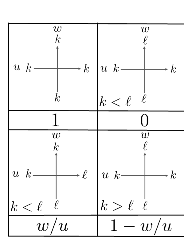
Figure 1: A graphical description of the $R$-matrix $R_{ij}(u,w)$ which is a $q=0$ degeneration of the $U_{q}(\widehat{sl_{m+1}})$ $R$-matrix (2.1), (2.2), (2.3). We display the elements of the $R$-matrix. The $R$-matrix is represented as two crossing arrows. The left and the up arrow represents the space $W_{i}$ and $W_{j}$, respectively. The top left figure represents ${}_{i}\langle k|\otimes{}_{j}\langle k|R(u,w)|k\rangle_{i}\otimes|k\rangle_{j}=1$, $0\leq k\leq m$. The top middle figure represents ${}_{i}\langle k|\otimes{}_{j}\langle\ell|R(u,w)|k\rangle_{i}\otimes|\ell\rangle_{j}=0$, $0\leq k<\ell\leq m$. The top right figure represents ${}_{i}\langle\ell|\otimes{}_{j}\langle k|R(u,w)|k\rangle_{i}\otimes|\ell\rangle_{j}=1$, $m\geq k>\ell\geq 0$. The bottom left figure represents ${}_{i}\langle\ell|\otimes{}_{j}\langle k|R(u,w)|k\rangle_{i}\otimes|\ell\rangle_{j}=w/u$, $0\leq k<\ell\leq m$. The bottom right figure represents ${}_{i}\langle k|\otimes{}_{j}\langle\ell|R(u,w)|k\rangle_{i}\otimes|\ell\rangle_{j}=1-w/u$, $m\geq k>\ell\geq 0$. All the other matrix elements which are not displayed in the figure above are identically zero.

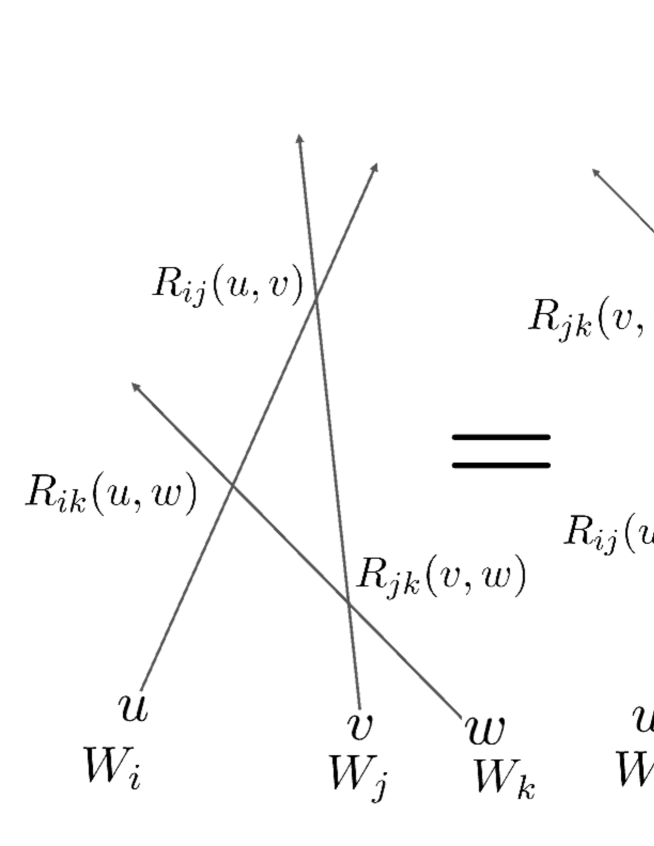
Figure 2: A graphical description of the Yang-Baxter relation $R_{ij}(u,v)R_{ik}(u,w)R_{jk}(v,w)=R_{jk}(v,w)R_{ik}(u,w)R_{ij}(u,v)\in\mathrm{End}(W_{i}\otimes W_{j}\otimes W_{k})$ (2.7). The left and right figure represents $R_{ij}(u,v)R_{ik}(u,w)R_{jk}(v,w)$ and $R_{jk}(v,w)R_{ik}(u,w)R_{ij}(u,v)$ respectively.

The $R$-matrix $R_{ij}(u,w)$ satisifies the Yang-Baxter relation (Figure 2)

$$R_{ij}(u,v)R_{ik}(u,w)R_{jk}(v,w)=R_{jk}(v,w)R_{ik}(u,w)R_{ij}(u,v).$$ (2.7)

We regard (2.7) as a relation on $W_{i}\otimes W_{j}\otimes W_{k}$ and view $R_{ij}(u,v)$, $R_{ik}(u,w)$ and $R_{jk}(v,w)$ as operators acting on $W_{i}\otimes W_{j}\otimes W_{k}$, which acts nontrivially on $W_{i}\otimes W_{j}$, $W_{i}\otimes W_{k}$ and $W_{j}\otimes W_{k}$ respectively, and acts as identity on $W_{k}$, $W_{j}$ and $W_{i}$ respectively.

More generally, we view (2.7) as a relation in a larger vector space $W_{1}\otimes\cdots\otimes W_{p}$ for an integer $p\geq 3$ and regard that $R_{ij}(u,v)$ acts nontrivially on $W_{i}$ and $W_{j}$, $R_{ik}(u,w)$ nontrivially on $W_{i}$ and $W_{k}$, $R_{jk}(v,w)$ nontrivially on $W_{j}$ and $W_{k}$, and each of them acts as identity on all the other spaces.

From the $R$-matrix, we construct the monodromy matrix $T_{a}(u)$

$$T_{a}(u) =R_{a,p}(u,1)\cdots R_{a1}(u,1),$$ (2.8)

which are operators acting on $W_{a}\otimes W_{1}\otimes\cdots\otimes W_{p}$. The $R$-matrix $R_{a,j}(u,1)$ $(1\leq j\leq p)$ acts nontrivially on $W_{a}$ and $W_{j}$ and as identity on the remaining spaces. All the $R$-matrices act nontrivially on $W_{a}$, and this space is traditionally called as the auxiliary space. We use alphabets, typlically $a$ to label this special space and denote the vector space as $W_{a}$. On the other hand, the other spaces $W_{1},\dots,W_{p}$ are called as quantum spaces.

Since the monodromy matrix $T_{a}(u)$ acts on $W_{a}\otimes W_{1}\otimes\cdots\otimes W_{p}$ whose dimension is $(m+1)^{p+1}$, this monodromy matrix can be regarded as a $(m+1)^{p+1}\times(m+1)^{p+1}$ matrix.

We now consider the matrix elements of the monodromy matrix with respect the auxiliary space $W_{a}$

$$T_{ij}(u):={}_{a}\langle j|T_{a}(u)|i\rangle_{a},\ \ \ i,j=0,\dots,m.$$ (2.9)

Each of the elements $T_{ij}(u)$ act on $W_{1}\otimes\cdots\otimes W_{p}$ and can be regarded as $(m+1)^{p}\times(m+1)^{p}$ matrices.

In this paper, we use the following ones

$$B_{k}(u): =T_{mk}(u),\ \ \ k=0,1,\dots,m-1,$$ (2.10)

$$D_{m}(u): =T_{mm}(u).$$ (2.11)

See Figure 3 for graphical descriptions of the operators $B_{k}(u)$ ($k=0,1,\dots,m-1$) and $D_{m}(u)$.

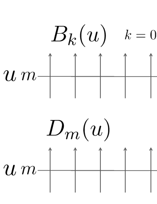
Figure 3: The operators $B_{k}(u)=T_{mk}(u)={}_{a}\langle k|T_{a}(u)|m\rangle_{a}$ ($k=0,1,\dots,m-1$) (2.10) (top) and $D_{m}(u)=T_{mm}(u)={}_{a}\langle m|T_{a}(u)|m\rangle_{a}$ (2.11) (bottom).

3 Partition functions

We introduce three types of partition functions in this section. Let us first introduce notations for the basis of the space $W_{1}\otimes W_{2}\otimes\cdots\otimes W_{p}$ and its dual $W_{1}^{*}\otimes W_{2}^{*}\otimes\cdots\otimes W_{p}^{*}$. For an ordered set of integers $I=\{i_{1},i_{2},\dots,i_{p}\}$ satisfying $0\leq i_{1},i_{2},\dots,i_{p}\leq m$, we define $|I\rangle$ and $\langle I|$ as

$$|I\rangle =|i_{1}\rangle_{1}\otimes|i_{2}\rangle_{2}\otimes\cdots\otimes|i_{p}\rangle_{p}\in W_{1}\otimes W_{2}\otimes\cdots\otimes W_{p},$$ (3.1)

$$\langle I| ={}_{1}\langle i_{1}|\otimes{}_{2}\langle i_{2}|\otimes\cdots\otimes{}_{p}\langle i_{p}|\in W_{1}^{*}\otimes W_{2}^{*}\otimes\cdots\otimes W_{p}^{*}.$$ (3.2)

$\{|I\rangle\ |\ 0\leq i_{1},i_{2},\dots,i_{p}\leq m\}$ and $\{\langle I|\ |\ 0\leq i_{1},i_{2},\dots,i_{p}\leq m\}$ forms a standard basis of $W_{1}\otimes W_{2}\otimes\cdots\otimes W_{p}$ and $W_{1}^{*}\otimes W_{2}^{*}\otimes\cdots\otimes W_{p}^{*}$ respectively.

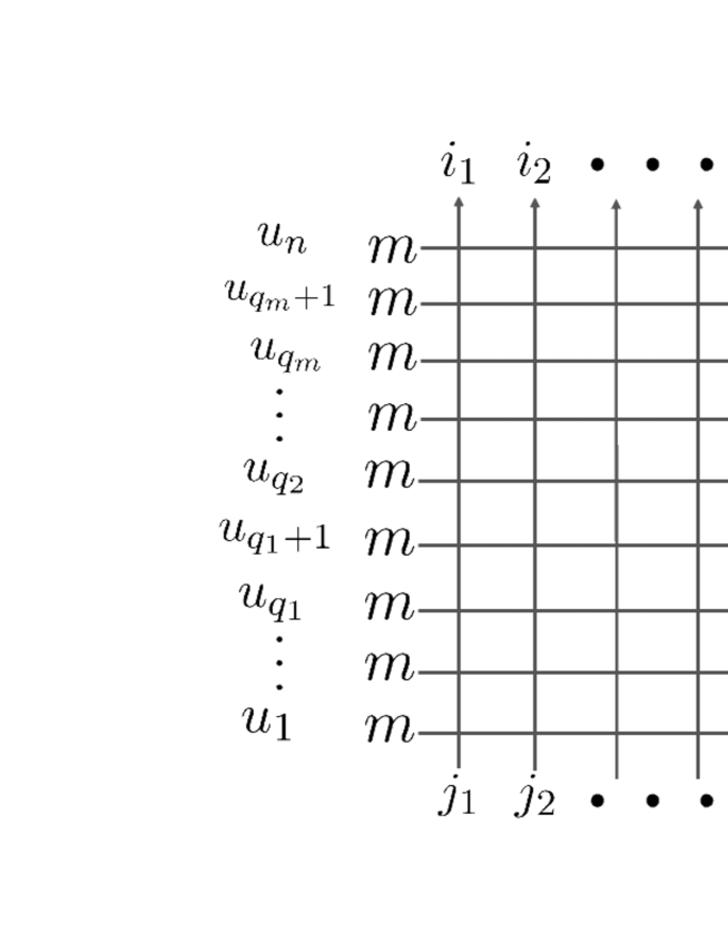
Figure 4: The partition functions $F_{IJ}(u_{1},\dots,u_{n})$ (3.3). The top sequence of integers corresponds to $\langle I|$. The first $n-q_{m}$ rows correspond to $B_{0}(u_{q_{m}+1}),\dots,B_{0}(u_{n})$. The next $q_{m}-q_{m-1}$ rows correspond to $B_{1}(u_{q_{m-1}+1}),\dots,B_{1}(u_{q_{m}})$, and so on. The bottom sequence of integers corresponds to $|J\rangle$.

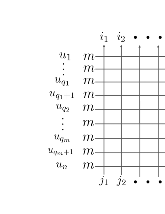
Figure 5: The partition functions $G_{IJ}(u_{1},\dots,u_{n})$ (3.4). Note that since the ordering of operators is reversed from $F_{IJ}(u_{1},\dots,u_{n})$, the boundary condition on the right is reversed from Figure 4. We also reversed the ordering of spectral parameters. However, the ordering of the spectral parameters do not matter since $G_{IJ}(u_{1},\dots,u_{n})$ are symmetric with respect to $u_{1},\dots,u_{n}$. This symmetry can be understood for example by showing that $G_{IJ}(u_{1},\dots,u_{n})$ are equivalent to the third type of partition functions $H_{IJ}(u_{1},\dots,u_{n})$ constructed only from $B_{0}$-operators. Then the symmetry follows from the commutativity of the $B_{0}$-operators.

We also introduce a set of integers $q_{1},q_{2},\dots,q_{m}$ satisfying $q_{0}:=0<q_{1}<q_{2}<\cdots<q_{m}<q_{m+1}:=n$.

Using the operators $B_{k}(u)$ ($k=0,1,\dots,m-1$) (2.10), $D_{m}(u)$ (2.11) and (dual) basis vectors $\langle I|$, $|J\rangle$, we introduce the first type of partition functions $F_{IJ}(u_{1},\dots,u_{n})$ as (see Figure 4 for a graphical description)

$$F_{IJ}(u_{1},\dots,u_{n})$$

$$= \langle I|\prod_{j=q_{m}+1}^{n}B_{0}(u_{j})\prod_{j=q_{m-1}+1}^{q_{m}}B_{1}(u_{j})\cdots\prod_{j=q_{1}+1}^{q_{2}}B_{m-1}(u_{j})\prod_{j=1}^{q_{1}}D_{m}(u_{j})|J\rangle.$$ (3.3)

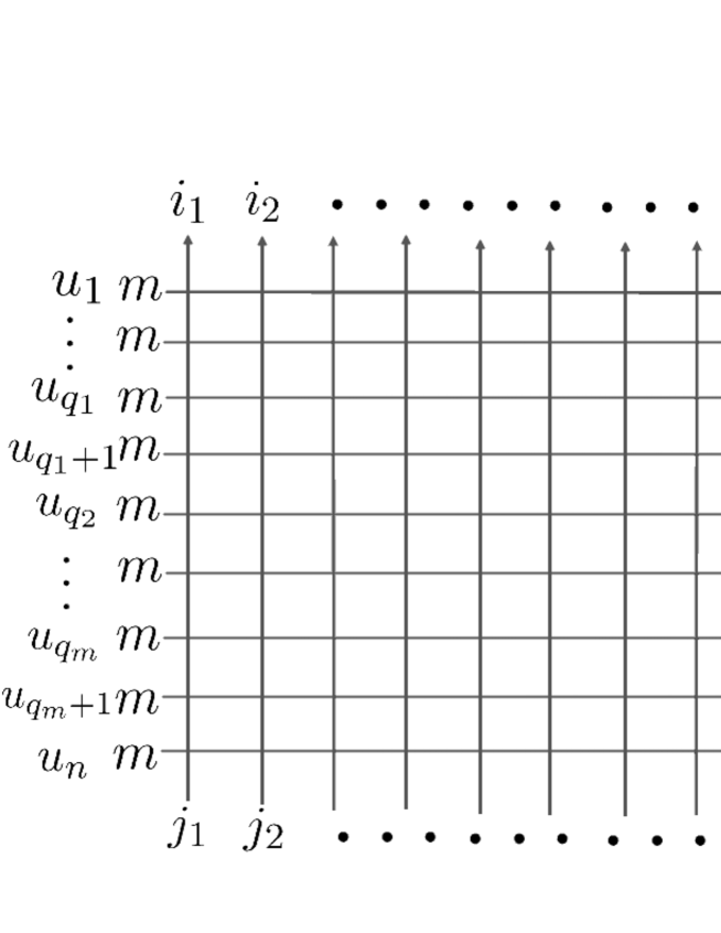
Figure 6: The partition functions $H_{IJ}(u_{1},\dots,u_{n})$ (3.10). Note the rectangular grid is wider than the ones for $F_{IJ}(u_{1},\dots,u_{n})$ and $G_{IJ}(u_{1},\dots,u_{n})$. $q_{m}$ columns are added, and integers are also added in top and bottom of those columns as in the figure. Note also that the integers in the right boundary are all 0, which means that the partition functions are constructed only using the $B_{0}$-operators. Since the $B_{0}$-operators are commutative, this implies that $H_{IJ}(u_{1},\dots,u_{n})$ are symmetric with respect to $u_{1},\dots,u_{n}$.

We next introduce the second type of partition functions $G_{IJ}(u_{1},\dots,u_{n})$ as

$$G_{IJ}(u_{1},\dots,u_{n})$$

$$= \langle I|\prod_{j=1}^{q_{1}}D_{m}(u_{j})\prod_{j=q_{1}+1}^{q_{2}}B_{m-1}(u_{j})\cdots\prod_{j=q_{m-1}+1}^{q_{m}}B_{1}(u_{j})\prod_{j=q_{m}+1}^{n}B_{0}(u_{j})|J\rangle.$$ (3.4)

Note the order of operators to define $G_{IJ}(u_{1},\dots,u_{n})$ in (3.4) is reversed from the one for $F_{IJ}(u_{1},\dots,u_{n})$ (3.3). See Figure 5 for a graphical description.

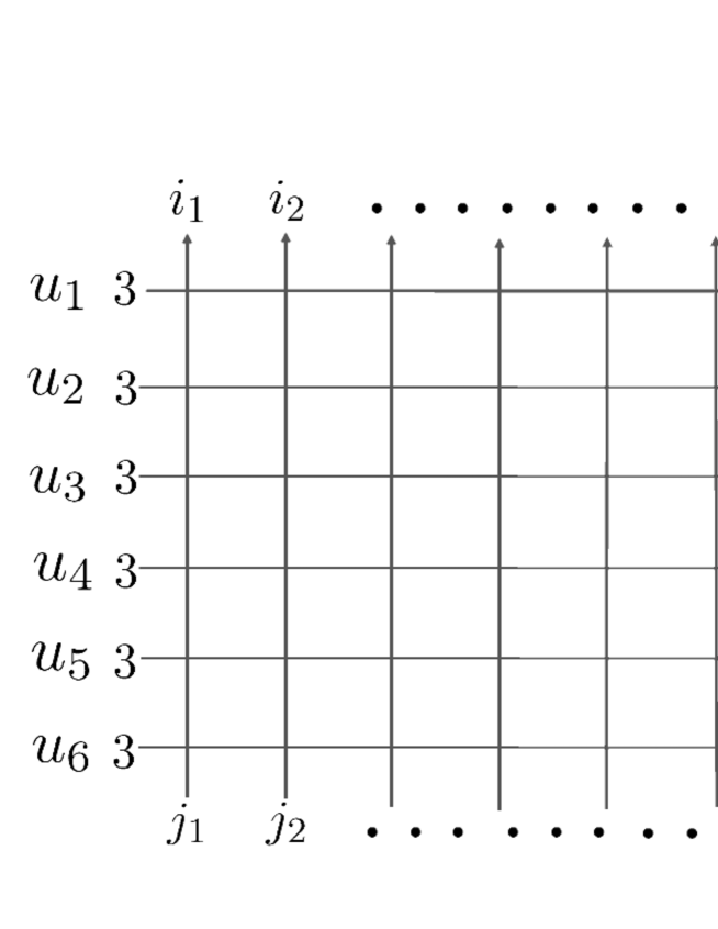
Figure 7: The partition functions $H_{IJ}(u_{1},\dots,u_{n})$ corresponding to $m=3$, $n=6$, $q_{1}=2$, $q_{2}=3$, $q_{3}=5$.

Figure 8: The partition functions $H_{IJ}(u_{1},\dots,u_{n})$ corresponding to $m=3$, $n=6$, $q_{1}=2$, $q_{2}=3$, $q_{3}=5$. Using Figure 1, one observes that only one configuration is allowed in the rightmost $q_{m}$ columns. The remaining part is nothing but the partition functions $G_{IJ}(u_{1},\dots,u_{n})$.

We also introduce the third type of partition functions which is equivalent to the second type $G_{IJ}(u_{1},\dots,u_{n})$. The third type uses only $B_{0}$-operators and acts on a larger quantum space. Let us define $B_{0}^{(p,q_{1},q_{2},\dots,q_{m})}(u)$ as the $B_{0}$-operator acting on $W_{1}\otimes W_{2}\otimes\cdots\otimes W_{p+q_{m}}$

$$B_{0}^{(p,q_{1},q_{2},\dots,q_{m})}(u)={}_{a}\langle 0|R_{a,p+q_{m}}(u,1)\cdots R_{a2}(u,1)R_{a1}(u,1)|m\rangle_{a}.$$ (3.5)

We also extend the (dual) basis vectors $|I\rangle\in W_{1}\otimes W_{2}\otimes\cdots\otimes W_{p}$ and $\langle J|\in W_{1}^{*}\otimes W_{2}^{*}\otimes\cdots\otimes W_{p}^{*}$ to (dual) vectors in $W_{1}\otimes W_{2}\otimes\cdots\otimes W_{p+q_{m}}$ and $W_{1}^{*}\otimes W_{2}^{*}\otimes\cdots\otimes W_{p+q_{m}}^{*}$. For ordered sets of integers $I=\{i_{1},i_{2},\dots,i_{p}\}$ ($0\leq i_{1},i_{2},\dots,i_{p}\leq m$) and $J=\{j_{1},j_{2},\dots,j_{p}\}$ ($0\leq j_{1},j_{2},\dots,j_{p}\leq m$), we define $\langle\widetilde{I}|\in W_{1}^{*}\otimes W_{2}^{*}\otimes\cdots\otimes W_{p+q_{m}}^{*}$ and $|\widetilde{J}\rangle\in W_{1}\otimes W_{2}\otimes\cdots\otimes W_{p+q_{m}}$ as

$$\langle\widetilde{I}| =\langle I|\otimes\langle m^{q_{1}},(m-1)^{q_{2}-q_{1}},\dots,2^{q_{m-1}-q_{m-2}},1^{q_{m}-q_{m-1}}|,$$ (3.6)

$$|\widetilde{J}\rangle =|J\rangle\otimes|0^{q_{m}}\rangle,$$ (3.7)

where

$$|0^{q_{m}}\rangle=|0\rangle_{p+1}\otimes\cdots\otimes|0\rangle_{p+q_{m}},$$ (3.8)

$$\langle m^{q_{1}},(m-1)^{q_{2}-q_{1}},\dots,2^{q_{m-1}-q_{m-2}},1^{q_{m}-q_{m-1}}|$$

$$= ({}_{p+1}\langle m|\otimes\cdots\otimes{}_{p+q_{1}}\langle m|)\otimes({}_{p+q_{1}+1}\langle m-1|\otimes\cdots\otimes{}_{p+q_{2}}\langle m-1|)$$

$$\otimes\cdots\otimes({}_{p+q_{m-2}+1}\langle 2|\otimes\cdots\otimes{}_{p+q_{m-1}}\langle 2|)\otimes({}_{p+q_{m-1}+1}\langle 1|\otimes\cdots\otimes{}_{p+q_{m}}\langle 1|).$$ (3.9)

Using $B_{0}^{(p,q_{1},q_{2},\dots,q_{m})}(u)$, $\langle\widetilde{I}|$ and $|\widetilde{J}\rangle$, we introduce the third type of partition functions $H_{IJ}(u_{1},\dots,u_{n})$ as (Figure 6)

$$H_{IJ}(u_{1},\dots,u_{n})=\langle\widetilde{I}|B_{0}^{(p,q_{1},q_{2},\dots,q_{m})}(u_{1})B_{0}^{(p,q_{1},q_{2},\dots,q_{m})}(u_{2})\cdots B_{0}^{(p,q_{1},q_{2},\dots,q_{m})}(u_{n})|\widetilde{J}\rangle.$$ (3.10)

We can show that the partition functions $G_{IJ}(u_{1},\dots,u_{n})$ (3.4) are the same with $H_{IJ}(u_{1},\dots,u_{n})$ (3.10), i.e. they are represented by the same symmetric functions.

Lemma 3.1.

The following relation holds:

$$G_{IJ}(u_{1},\dots,u_{n})=H_{IJ}(u_{1},\dots,u_{n}).$$ (3.11)

Proof.

The equality (3.11) can be shown graphically in the same way with Appendix C in [35]. Let us illustrate this by an example. Set $m=3$, $n=6$, $q_{1}=2$, $q_{2}=3$, $q_{3}=5$, which Figure 7 corresponds to this example. We first look the $R$-matrix at the upper right corner. The output of the $R$-matrix of the auxiliary space and quantum space $W_{p+q_{m}}$ is 0 and 1 respectively. Looking the top middle and top right figures in Figure 1, one notes that the input of auxiliary space and quantum space $W_{p+q_{m}}$ must be fixed to 1 and 0 respectively. This means that the integers around the vertex at the upper right corner are fixed as depicted in Figure 8. Next, we look the $R$-matrix which is left to the one which we have just investigated. The outputs of the auxiliary space and quantum space $W_{p+q_{m}-1}$ are both 1. Looking the top left figure in Figure 1, we note the inputs of the auxiliary space and quantum space $W_{p+q_{m}-1}$ must be fixed both to 1. The integers around the vertex corresponding to this $R$-matrix are all fixed to 1. Continuing this observation, we find only one configuration is allowed in the rightmost $q_{m}$ columns as Figure 8. The remaining part is nothing but $G_{IJ}(u_{1},\dots,u_{n})$, hence we find $H_{IJ}(u_{1},\dots,u_{n})$ is equal to $G_{IJ}(u_{1},\dots,u_{n})$ multiplied by all the $R$-matrix elements which come from the frozen rightmost $q_{m}$ columns. Since all the $R$-matrix elements which appear in those columns are 1, we conclude $H_{IJ}(u_{1},\dots,u_{n})=G_{IJ}(u_{1},\dots,u_{n})$. ∎

4 Yang-Baxter algebra, symmetries and multiple commutation relations

In this section, we show the key multiple commutation relations of the Yang-Baxter algebra. Let us first recall the basic commutation relations for the operators $T_{ij}(u)$ which are matrix elements of the monodromy matrix with respect to the auxiliary space. For readers unfamiliar with this argument, we refer to [35] for example for a detailed account where the meaning of the conventions used in quantum integrable models and quantum groups are explained (on which space the operators act, for example).

From the Yang-Baxter relation (2.7), the intertwining relation between monodromy matrices follows

$$R_{ab}(u_{1},u_{2})T_{a}(u_{1})T_{b}(u_{2})=T_{b}(u_{2})T_{a}(u_{1})R_{ab}(u_{1},u_{2}).$$ (4.1)

The intertwining relation (4.1), which is often called as the $RTT$ relation, can be regarded as an equality between matrices, and equalities between the matrix elements of both hand sides are actually commutation relations among the matrix elements $T_{ij}(u)$ of the monodromy matrix. The commutation relations we need in this paper are the following:

$$D_{m}(u_{1})B_{j}(u_{2}) =\frac{1}{1-u_{2}/u_{1}}B_{j}(u_{2})D_{m}(u_{1})+\frac{1}{1-u_{1}/u_{2}}B_{j}(u_{1})D_{m}(u_{2}),\ \ \ j=0,1,\dots,m-1,$$ (4.2)

$$B_{j}(u_{1})B_{k}(u_{2}) =\frac{1}{1-u_{2}/u_{1}}B_{k}(u_{2})B_{j}(u_{1})+\frac{1}{1-u_{1}/u_{2}}B_{k}(u_{1})B_{j}(u_{2}),\ \ \ 0\leq k<j\leq m-1,$$ (4.3)

$$D_{m}(u_{1})B_{j}(u_{2}) =D_{m}(u_{2})B_{j}(u_{1}),\ \ \ j=0,1,\dots,m-1,$$ (4.4)

$$B_{j}(u_{1})B_{k}(u_{2}) =B_{j}(u_{2})B_{k}(u_{1}),\ \ \ 0\leq k\leq j\leq m-1,$$ (4.5)

$$D_{m}(u_{1})D_{m}(u_{2}) =D_{m}(u_{2})D_{m}(u_{1}).$$ (4.6)

From the $j=k$ case of (4.5) and (4.6), the following symmetries hold for the partition functions $F_{IJ}(u_{1},\dots,u_{n})$ (3.3).

Lemma 4.1.

$F_{IJ}(u_{1},\dots,u_{n})$ are symmetric with respect to $u_{q_{j-1}+1},\dots,u_{q_{j}}$ for each j=1,…,m+1. Here we set $q_{0}:=0$, $q_{m+1}:=n$.

The $j=k$ case of (4.5) and (4.6) also imply that the same symmetries hold for $G_{IJ}(u_{1},\dots,u_{n})$ (3.4).

Lemma 4.2.

$G_{IJ}(u_{1},\dots,u_{n})$ are symmetric with respect to $u_{q_{j-1}+1},\dots,u_{q_{j}}$ for each j=1,…,m+1.

We note a higher symmetry holds for $G_{IJ}(u_{1},\dots,u_{n})$. These partition functions are actually fully symmetric with respect to $u_{1},\dots,u_{n}$. To see this, we first note from the $j=k=0$ case of (4.5) that the third type of partition functions $H_{IJ}(u_{1},\dots,u_{n})$ constructed using only $B_{0}$-operators (3.10) are fully symmetric.

Lemma 4.3.

$H_{IJ}(u_{1},\dots,u_{n})$ are symmetric with respect to $u_{1},\dots,u_{n}$.

Combining Lemma 4.3 with Lemma 3.1, we note $G_{IJ}(u_{1},\dots,u_{n})$ are fully symmetric.

Lemma 4.4.

$G_{IJ}(u_{1},\dots,u_{n})$ are symmetric with respect to $u_{1},\dots,u_{n}$.

Let us now show the multiple commutation relations from the basic commutation relations (4.2), (4.3), (4.4), (4.5) and (4.6). The simplest case $m=1$ was previously used in [35, 82] to derive a skew generalization of the identities for (factorial) Schur/Grothendieck polynomials by Fehér-Némethi-Rimányi and Guo-Sun [83, 84].

Proposition 4.5.

The following multiple commutation relations hold:

$$\displaystyle\prod_{j=1}^{q_{1}}D_{m}(u_{j})\prod_{j=q_{1}+1}^{q_{2}}B_{m-1}(u_{j})\cdots\prod_{j=q_{m-1}+1}^{q_{m}}B_{1}(u_{j})\prod_{j=q_{m}+1}^{n}B_{0}(u_{j})$$

$$= \sum_{\overline{w}\in S_{n}/S_{q_{1}}\times S_{q_{2}-q_{1}}\times\cdots\times S_{n-q_{m}}}w\cdot\Bigg{[}\frac{1}{\prod_{k=1}^{m}\prod_{q_{k-1}<i\leq q_{k}}\prod_{q_{k}<j\leq n}(1-u_{j}/u_{i})}$$

$$\times\prod_{j=q_{m}+1}^{n}B_{0}(u_{j})\prod_{j=q_{m-1}+1}^{q_{m}}B_{1}(u_{j})\cdots\prod_{j=q_{1}+1}^{q_{2}}B_{m-1}(u_{j})\prod_{j=1}^{q_{1}}D_{m}(u_{j})\Bigg{]}.$$ (4.7)

Here, $w$ in the right hand side of (4.7) acts as permutation on the the spectral parameters $(u_{1},u_{2},\dots,u_{n})$, and the sum is over all representatives of elements of the fixed subgroup $S_{n}/S_{q_{1}}\times S_{q_{2}-q_{1}}\times\cdots\times S_{n-q_{m}}$ of the symmetric group $S_{n}$.

Proof.

We illustrate the simplest nontrivial case $m=2$ beyond $m=1$, which can be applied to the cases $m>2$ as well. We can apply the argument in [59] for this type of higher rank multiple commutation relations. Let us write down the commutation relations more explicitly. Each $\overline{w}\in S_{n}/S_{q_{1}}\times S_{q_{2}-q_{1}}\times S_{n-q_{2}}$ can be represented as a tuple $(S^{(0)},S^{(1)},S^{(2)})$ where $S^{(0)}$, $S^{(1)}$, $S^{(2)}$ are unordered sets of integers such that

$$|S^{(0)}|=q_{1},\ \ \ |S^{(1)}|=q_{2}-q_{1},\ \ \ |S^{(2)}|=n-q_{2},\ \ \ S^{(0)}\cup S^{(1)}\cup S^{(2)}=\{1,2,\dots,n\}.$$ (4.8)

Then we note the case $m=2$ of (4.7) can be written as

$$\displaystyle\prod_{j=1}^{q_{1}}D_{2}(u_{j})\prod_{j=q_{1}+1}^{q_{2}}B_{1}(u_{j})\prod_{j=q_{2}+1}^{n}B_{0}(u_{j})$$

$$= \sum_{(S^{(0)},S^{(1)},S^{(2)})}\prod_{\begin{subarray}{c}i\in S^{(0)}\\ j\in S^{(1)}\end{subarray}}\frac{1}{1-u_{j}/u_{i}}\prod_{\begin{subarray}{c}i\in S^{(0)}\\ j\in S^{(2)}\end{subarray}}\frac{1}{1-u_{j}/u_{i}}\prod_{\begin{subarray}{c}i\in S^{(1)}\\ j\in S^{(2)}\end{subarray}}\frac{1}{1-u_{j}/u_{i}}$$

$$\times\prod_{j\in S^{(2)}}B_{0}(u_{j})\prod_{j\in S^{(1)}}B_{1}(u_{j})\prod_{j\in S^{(0)}}D_{2}(u_{j}).$$ (4.9)

Here, the sum in the right hand side of (4.9) is over all tuples $(S^{(0)},S^{(1)},S^{(2)})$ of unordered sets of integers $S^{(0)}$, $S^{(1)}$, $S^{(2)}$ satisfying (4.8).

Let us show (4.9). First, starting from the left hand side, we reverse the order of the types of the operators using (4.2), (4.3), (4.5) and (4.6) and move all $D_{2}$-operators to the right of $B_{0}$- and $B_{1}$-operators, and move all $B_{0}$-operators to the left of $B_{1}$- and $D_{2}$-operators. We note that the operator part of all the terms which appear from this process can be expressed as

$$\prod_{j\in S^{(2)}}B_{0}(u_{j})\prod_{j\in S^{(1)}}B_{1}(u_{j})\prod_{j\in S^{(0)}}D_{2}(u_{j}),$$ (4.10)

for some tuple $(S^{(0)},S^{(1)},S^{(2)})$ of unordered sets of integers $S^{(0)}$, $S^{(1)}$, $S^{(2)}$ satisfying (4.8).

We extract the coefficient of (4.10) for a fixed tuple $(S^{(0)},S^{(1)},S^{(2)})$ as follows. We first use (4.4) and (4.5) repeatedly and rewrite the left hand side of (4.9) as

$$\prod_{j\in S^{(0)}}D_{2}(u_{j})\prod_{j\in S^{(1)}}B_{1}(u_{j})\prod_{j\in S^{(2)}}B_{0}(u_{j}).$$ (4.11)

We then use either (4.2) or (4.3) repeatedly and reverse the order of the types of operators. In this process, we always choose the first term of the right hand side of (4.2) and (4.3) when commuting the $B_{0}$-, $B_{1}$- and $D_{2}$-operators to extract the coefficient of (4.10). This is since if we once use the second term of the right hand side of (4.2) or (4.3), we get other operators. From this process, we find the coefficient of the operator is given by $\displaystyle\prod_{\begin{subarray}{c}i\in S^{(0)}\\ j\in S^{(1)}\end{subarray}}\frac{1}{1-u_{j}/u_{i}}\prod_{\begin{subarray}{c}i\in S^{(0)}\\ j\in S^{(2)}\end{subarray}}\frac{1}{1-u_{j}/u_{i}}\prod_{\begin{subarray}{c}i\in S^{(1)}\\ j\in S^{(2)}\end{subarray}}\frac{1}{1-u_{j}/u_{i}}$, hence (4.9) follows.

∎

5 Yang-Baxter algebra and $K$-theoretic Gysin map for partial flag bundles

In this section, combining the multiple commutation relations of the Yang-Baxter algebra derived in the last section and description of the $K$-theoretic Gysin map for flag bundles using symmetrizing operators, we show the first and second type of partition functions on a rectangular grid, which corresponds to Grothendieck classes of the Grothendieck group of the partial flag bundles and a nonsingular variety respectively, are directly connected via the $K$-theoretic Gysin map. First we collect results from the geometry side. There are various approaches to the Gysin map. See [85, 86, 87, 88, 89, 90, 91, 92, 93, 94, 95, 96, 97, 98, 99, 100, 101, 102, 103, 104, 105, 106, 107, 108, 109, 110, 111] as well as aforementioned articles for examples.

For a smooth scheme $X$, $K^{0}(X)$ denotes the Grothendieck group of locally free coherent sheaves on $X$. For $\mathcal{E}$ a locally free sheaf on $X$, we denote its class in $K^{0}(X)$ by $[\mathcal{E}]$.

Let $E\longrightarrow X$ be a complex vector bundle of rank $n$. We denote the bundles of flags of subspaces of dimensions $q_{1},\dots,q_{m}$ ($q_{0}:=0<q_{1}<q_{2}<\cdots<q_{m}<q_{m+1}:=n$) as $\pi_{q_{1},\dots,q_{m}}:\mathcal{F\ell}_{q_{1},\dots,q_{m}}(E)\longrightarrow X$. There exists a universal flag of subbundles of the pullback $\pi_{q_{1},\dots,q_{m}}^{*}(E)$ of $E$ on $\mathcal{F\ell}_{q_{1},\dots,q_{m}}(E)$,

$$U_{q_{0}}:=0\subsetneq U_{q_{1}}\subsetneq U_{q_{2}}\subsetneq\cdots\subsetneq U_{q_{m}}\subsetneq U_{q_{m+1}}:=\pi_{q_{1},\dots,q_{m}}^{*}(E),$$ (5.1)

where the rank of subbundle $U_{q_{i}}$ is $q_{i}$ for $i=0,1,\dots,m+1$.

The special case $m=n-1$, $q_{j}=j\ (j=1,2,\dots,n-1)$ of the flag bundle $\pi_{1,2,\dots,n-1}:\mathcal{F\ell}_{1,2,\dots,n-1}(E)\longrightarrow X$ is called the complete flag bundle, on which there exists the universal flag of subbundles

$$0=U_{0}\subsetneq U_{1}\subsetneq\cdots\subsetneq U_{n-1}\subsetneq\pi_{1,2,\dots,n-1}^{*}(E).$$ (5.2)

We denote the class of the dual line bundle $(U_{i}/U_{i-1})^{\vee}$ as $u_{i}$ in this section.

It is known that there are ways to describe Gysin map using symmetrizing operators. See [86, 93, 94, 95, 109, 111] for example. One of the latest results is for the generalized cohomology theory by Nakagawa-Naruse ([109] Thm 4.10, [111] Remark 3.9). Specializing to the $K$-theory case is the following.

Theorem 5.1.

Let $\pi_{q_{1},\dots,q_{m}}$ be the partial flag bundle $\pi_{q_{1},\dots,q_{m}}:\mathcal{F\ell}_{q_{1},\dots,q_{m}}(E)\longrightarrow X$. The pushforward $\pi_{q_{1},\dots,q_{m}*}:K^{0}(\mathcal{F\ell}_{q_{1},\dots,q_{m}}(E))\longrightarrow K^{0}(X)$ of a symmetric polynomial $f(1-t_{1}^{-1},\dots,1-t_{n}^{-1})\in K^{0}(X)[t_{1}^{-1},\dots,t_{n}^{-1}]^{S_{q_{1}}\times S_{q_{2}-q_{1}}\times\cdots\times S_{n-q_{m}}}$ is given by

$$\pi_{q_{1},\dots,q_{m}*}(f(1-u_{1}^{-1},\dots,1-u_{n}^{-1}))$$

$$= \sum_{\overline{w}\in S_{n}/S_{q_{1}}\times S_{q_{2}-q_{1}}\times\cdots\times S_{n-q_{m}}}w\cdot\Bigg{[}\frac{f(1-u_{1}^{-1},\dots,1-u_{n}^{-1})}{\prod_{k=1}^{m}\prod_{q_{k-1}<i\leq q_{k}}\prod_{q_{k}<j\leq n}(1-u_{j}/u_{i})}\Bigg{]}.$$ (5.3)

Here, $w$ in the right hand side of (5.3) acts as permutation on the Grothendieck roots $(u_{1},u_{2},\dots,u_{n})$, and the sum is over all representatives of elements of the fixed subgroup $S_{n}/S_{q_{1}}\times S_{q_{2}-q_{1}}\times\cdots\times S_{n-q_{m}}$ of the symmetric group $S_{n}$.

We show the following formula for the $K$-theoretic Gysin map, connecting two higher rank partition funtions $F_{IJ}(u_{1},\dots,u_{n})$ (3.3) and $G_{IJ}(u_{1},\dots,u_{n})$ (3.4).

Theorem 5.2.

Let $\pi_{q_{1},\dots,q_{m}}$ be the partial flag bundle $\pi_{q_{1},\dots,q_{m}}:\mathcal{F\ell}_{q_{1},\dots,q_{m}}(E)\longrightarrow X$. The pushforward $\pi_{q_{1},\dots,q_{m}*}:K^{0}(\mathcal{F\ell}_{q_{1},\dots,q_{m}}(E))\longrightarrow K^{0}(X)$ of $F_{IJ}(u_{1},\dots,u_{n})$ is given by

$$\pi_{q_{1},\dots,q_{m}*}(F_{IJ}(u_{1},\dots,u_{n}))=G_{IJ}(u_{1},\dots,u_{n}).$$ (5.4)

Proof.

We first note that $F_{IJ}(u_{1},\dots,u_{n})$ (3.3) are polynomials in $u_{1}^{-1},\dots,u_{n}^{-1}$ with integer coefficients. This is since partition functions are constructed from $R$-matrices, which means that in principle, each $F_{IJ}(u_{1},\dots,u_{n})$ can be expressed as a sum of products of matrix elements of the $R$-matrices, which are either $0,1,u_{j}^{-1}\ (j=1,\dots,n)$ or $1-u_{j}^{-1}\ (j=1,\dots,n)$, and expanding the expression, we note $F_{IJ}(u_{1},\dots,u_{n})$ are polynomials in $u_{1}^{-1},\dots,u_{n}^{-1}$. Also note the symmetries stated in Lemma 4.1: $F_{IJ}(u_{1},\dots,u_{n})$ are symmetric with respect to $u_{q_{j-1}+1},\dots,u_{q_{j}}$ for each $j=1,\dots,m+1$.

Applying the description of the $K$-theoretic Gysin map using symmetrizing operators (5.3) to $F_{IJ}(u_{1},\dots,u_{n})$, we have

$$\pi_{q_{1},\dots,q_{m}*}(F_{IJ}(u_{1},\dots,u_{n}))$$

$$= \pi_{q_{1},\dots,q_{m}*}(\langle I|\prod_{j=q_{m}+1}^{n}B_{0}(u_{j})\prod_{j=q_{m-1}+1}^{q_{m}}B_{1}(u_{j})\cdots\prod_{j=q_{1}+1}^{q_{2}}B_{m-1}(u_{j})\prod_{j=1}^{q_{1}}D_{m}(u_{j})|J\rangle)$$

$$= \sum_{\overline{w}\in S_{n}/S_{q_{1}}\times S_{q_{2}-q_{1}}\times\cdots\times S_{n-q_{m}}}w\cdot\Bigg{[}\frac{1}{\prod_{k=1}^{m}\prod_{q_{k-1}<i\leq q_{k}}\prod_{q_{k}<j\leq n}(1-u_{j}/u_{i})}$$

$$\langle I|\prod_{j=q_{m}+1}^{n}B_{0}(u_{j})\prod_{j=q_{m-1}+1}^{q_{m}}B_{1}(u_{j})\cdots\prod_{j=q_{1}+1}^{q_{2}}B_{m-1}(u_{j})\prod_{j=1}^{q_{1}}D_{m}(u_{j})|J\rangle\Bigg{]}.$$ (5.5)

Since the (dual) basis vectors $|J\rangle$ and $\langle I|$ in (5.5) are independent of $w$, we can move them out to get

$$\pi_{q_{1},\dots,q_{m}*}(F_{IJ}(u_{1},\dots,u_{n}))$$

$$= \langle I|\sum_{\overline{w}\in S_{n}/S_{q_{1}}\times S_{q_{2}-q_{1}}\times\cdots\times S_{n-q_{m}}}w\cdot\Bigg{[}\frac{1}{\prod_{k=1}^{m}\prod_{q_{k-1}<i\leq q_{k}}\prod_{q_{k}<j\leq n}(1-u_{j}/u_{i})}$$

$$\prod_{j=q_{m}+1}^{n}B_{0}(u_{j})\prod_{j=q_{m-1}+1}^{q_{m}}B_{1}(u_{j})\cdots\prod_{j=q_{1}+1}^{q_{2}}B_{m-1}(u_{j})\prod_{j=1}^{q_{1}}D_{m}(u_{j})\Bigg{]}|J\rangle.$$ (5.6)

We then apply the key multiple commutation relations of the Yang-Baxter algebra (4.7) to (5.6) and get

$$\pi_{q_{1},\dots,q_{m}*}(F_{IJ}(u_{1},\dots,u_{n}))$$

$$= \langle I|\prod_{j=1}^{q_{1}}D_{m}(u_{j})\prod_{j=q_{1}+1}^{q_{2}}B_{m-1}(u_{j})\cdots\prod_{j=q_{m-1}+1}^{q_{m}}B_{1}(u_{j})\prod_{j=q_{m}+1}^{n}B_{0}(u_{j})|J\rangle$$

$$= G_{IJ}(u_{1},\dots,u_{n}).$$ (5.7)

∎

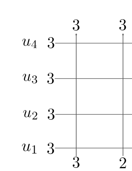
Figure 9: The partition functions $F_{IJ}(u_{1},\dots,u_{n})$ corresponding to (5.9). The figure represents the case $n=4$ ($m=3$).

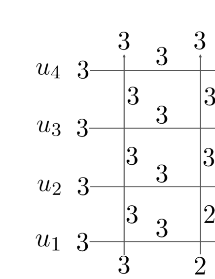
Figure 10: The partition functions $F_{IJ}(u_{1},\dots,u_{n})$ corresponding to (5.9). The figure represents the case $n=4$ ($m=3$). Using Figure 1, we find the product of the $R$-matrix elements in the first row is 1, the second row is $(1-u_{3}^{-1})$, the third row is $(1-u_{2}^{-1})^{2}$, the fourth row is $(1-u_{1}^{-1})^{3}$, and we find $F_{IJ}(u_{1},u_{2},u_{3},u_{4})=(1-u_{1}^{-1})^{3}(1-u_{2}^{-1})^{2}(1-u_{3}^{-1})$. For $n$ generic, we have $F_{IJ}(u_{1},\dots,u_{n})=\prod_{j=1}^{n}(1-u_{j}^{-1})^{n-j}$.

The following is known for complete flag bundles (see [109] for example)

$$\displaystyle\pi_{1,2,\dots,n-1*}\Bigg{(}\prod_{j=1}^{n}(1-u_{j}^{-1})^{n-j}\Bigg{)}=1.$$ (5.8)

As a check of Theorem 5.2, let us show this. This follows from the case $m=n-1$, $p=n$, $I=(n-1,n-1,\dots,n-1)$, $J=(n-1,n-2,\dots,0)$ of Theorem 5.2 as follows. In this case, $F_{IJ}(u_{1},\dots,u_{n})$ (3.3) is explicitly

$$F_{IJ}(u_{1},\dots,u_{n})={}_{1}\langle n-1|\otimes{}_{2}\langle n-1|\otimes\cdots\otimes{}_{n}\langle n-1|$$

$$\times B_{0}(u_{n})B_{1}(u_{n-1})\cdots B_{n-2}(u_{2})D_{n-1}(u_{1})|n-1\rangle_{1}\otimes|n-2\rangle_{2}\otimes\cdots\otimes|0\rangle_{n},$$ (5.9)

and is graphically represented as Figure 9. The figure represents the case $n=4$ ($m=3$). In the same way with showing Lemma 3.1 graphically, one observes that only one configuration is allowed. See Figure 10 for the case $n=4$ ($m=3$). From Figure 1 and Figure 10, one notes that the product of all the $R$-matrix elements appearing in this unique configuration is given by $\prod_{j=1}^{n}(1-u_{j}^{-1})^{n-j}$, i.e. we get

$$F_{IJ}(u_{1},\dots,u_{n})=\prod_{j=1}^{n}(1-u_{j}^{-1})^{n-j}.$$ (5.10)

Next, we compute $G_{IJ}(u_{1},\dots,u_{n})$ for this case. $G_{IJ}(u_{1},\dots,u_{n})$ (3.4) is explicitly

$$G_{IJ}(u_{1},\dots,u_{n})={}_{1}\langle n-1|\otimes{}_{2}\langle n-1|\otimes\cdots\otimes{}_{n}\langle n-1|$$

$$\times D_{n-1}(u_{1})B_{n-2}(u_{2})\cdots B_{1}(u_{n-1})B_{0}(u_{n})|n-1\rangle_{1}\otimes|n-2\rangle_{2}\otimes\cdots\otimes|0\rangle_{n},$$ (5.11)

and is graphically represented as Figure 11. The figure represents the case $n=4$ ($m=3$). One again notes that only one configuration is allowed, which is Figure 12. From Figure 1 and Figure 12, we find all the $R$-matrix elements appearing in this unique configuration is 1, hence we conclude

$$G_{IJ}(u_{1},\dots,u_{n})=1.$$ (5.12)

From (5.4), (5.10) and (5.12), we get (5.8).

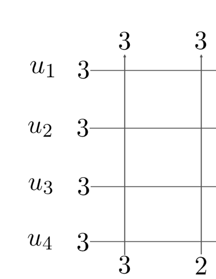
Figure 11: The partition functions $G_{IJ}(u_{1},\dots,u_{n})$ corresponding to (5.9). The figure represents the case $n=4$ ($m=3$).

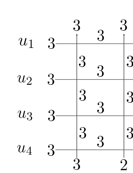
Figure 12: The partition functions $G_{IJ}(u_{1},\dots,u_{n})$ corresponding to (5.9). The figure represents the case $n=4$ ($m=3$). From Figure 1, we find all the $R$-matrix elements which appear in this unique configuration are 1, hence we note $G_{IJ}(u_{1},u_{2},u_{3},u_{4})=1$. This also holds for $n$ generic, i.e. we have $G_{IJ}(u_{1},\dots,u_{n})=1$.

6 Inhomogenous version

In this section, we discuss some generalization of algebraic and geometric aspects discussed in the previous sections. Let us introduce inhomogeneous parameters into the partition functions. One can see from the Yang-Baxter equation (2.7) that the intertwining relation

$$R_{ab}(u_{1},u_{2})T_{a}(u_{1}|w_{1},\dots,w_{p})T_{b}(u_{2}|w_{1},\dots,w_{p})$$

$$= T_{b}(u_{2}|w_{1},\dots,w_{p})T_{a}(u_{1}|w_{1},\dots,w_{p})R_{ab}(u_{1},u_{2}),$$ (6.1)

holds for the inhomogeneous version of the monodromy matrix (2.8)

$$T_{a}(u|w_{1},\dots,w_{p}) =R_{a,p}(u,w_{p})\cdots R_{a1}(u,w_{1}),$$ (6.2)

where parameters $w_{1},\dots,w_{p}$ are introduced. Recall the action of the $R$-matrix $R_{ij}(u,w)$ (2.1), (2.2), (2.3).

The matrix elements of the inhomogeneous monodromy matrix $T_{ij}(u|w_{1},\dots,w_{p}):={}_{a}\langle j|T_{a}(u|w_{1},\dots,w_{p})|i\rangle_{a}$ satisfy the same commutation relations with the homogeneous version which follow from the intertwining relation. For example, the relations (4.2), (4.3), (4.4), (4.5), (4.6) with $D_{m}(u),B_{k}(u)\ (k=0,1,\dots,m-1)$ replaced by $D_{m}(u|w_{1},\dots,w_{p}):=T_{mm}(u|w_{1},\dots,w_{p}),B_{k}(u|w_{1},\dots,w_{p}):=T_{mk}(u|w_{1},\dots,w_{p})\ (k=0,1,\dots,m-1)$ hold. Hence the inhomogeneous version of the multiple commutation relations (4.7) which are derived by those basic commutation relations

$$\displaystyle\prod_{j=1}^{q_{1}}D_{m}(u_{j}|w_{1},\dots,w_{p})\prod_{j=q_{1}+1}^{q_{2}}B_{m-1}(u_{j}|w_{1},\dots,w_{p})\cdots$$

$$\times\prod_{j=q_{m-1}+1}^{q_{m}}B_{1}(u_{j}|w_{1},\dots,w_{p})\prod_{j=q_{m}+1}^{n}B_{0}(u_{j}|w_{1},\dots,w_{p})$$

$$= \sum_{\overline{w}\in S_{n}/S_{q_{1}}\times S_{q_{2}-q_{1}}\times\cdots\times S_{n-q_{m}}}w\cdot\Bigg{[}\frac{1}{\prod_{k=1}^{m}\prod_{q_{k-1}<i\leq q_{k}}\prod_{q_{k}<j\leq n}(1-u_{j}/u_{i})}$$

$$\times\prod_{j=q_{m}+1}^{n}B_{0}(u_{j}|w_{1},\dots,w_{p})\prod_{j=q_{m-1}+1}^{q_{m}}B_{1}(u_{j}|w_{1},\dots,w_{p})\cdots$$

$$\times\prod_{j=q_{1}+1}^{q_{2}}B_{m-1}(u_{j}|w_{1},\dots,w_{p})\prod_{j=1}^{q_{1}}D_{m}(u_{j}|w_{1},\dots,w_{p})\Bigg{]},$$ (6.3)

hold as well.

We introduce the inhomogenous generalization of the first type of partition functions (3.3)

$$F_{IJ}(u_{1},\dots,u_{n}|w_{1},\dots,w_{p})$$

$$= \langle I|\prod_{j=q_{m}+1}^{n}B_{0}(u_{j}|w_{1},\dots,w_{p})\prod_{j=q_{m-1}+1}^{q_{m}}B_{1}(u_{j}|w_{1},\dots,w_{p})\cdots$$

$$\times\prod_{j=q_{1}+1}^{q_{2}}B_{m-1}(u_{j}|w_{1},\dots,w_{p})\prod_{j=1}^{q_{1}}D_{m}(u_{j}|w_{1},\dots,w_{p})|J\rangle,$$ (6.4)

and the second type of partition functions (3.4)

$$G_{IJ}(u_{1},\dots,u_{n}|w_{1},\dots,w_{p})$$

$$= \langle I|\prod_{j=1}^{q_{1}}D_{m}(u_{j}|w_{1},\dots,w_{p})\prod_{j=q_{1}+1}^{q_{2}}B_{m-1}(u_{j}|w_{1},\dots,w_{p})\cdots$$

$$\times\prod_{j=q_{m-1}+1}^{q_{m}}B_{1}(u_{j}|w_{1},\dots,w_{p})\prod_{j=q_{m}+1}^{n}B_{0}(u_{j}|w_{1},\dots,w_{p})|J\rangle.$$ (6.5)

At the algebraic level, the following relation between $F_{IJ}(u_{1},\dots,u_{n}|w_{1},\dots,w_{p})$ and $G_{IJ}(u_{1},\dots,u_{n}|w_{1},\dots,w_{p})$ follows from (6.3)

$$G_{IJ}(u_{1},\dots,u_{n}|w_{1},\dots,w_{p})$$

$$= \sum_{\overline{w}\in S_{n}/S_{q_{1}}\times S_{q_{2}-q_{1}}\times\cdots\times S_{n-q_{m}}}w\cdot\Bigg{[}\frac{F_{IJ}(u_{1},\dots,u_{n}|w_{1},\dots,w_{p})}{\prod_{k=1}^{m}\prod_{q_{k-1}<i\leq q_{k}}\prod_{q_{k}<j\leq n}(1-u_{j}/u_{i})}\Bigg{]}.$$ (6.6)

For $I$ and $J$ generic, the inhomogeneous version of partition functions $F_{IJ}(u_{1},\dots,u_{n}|w_{1},\dots,w_{p})$ and $G_{IJ}(u_{1},\dots,u_{n}|w_{1},\dots,w_{p})$ are not symmetric with respect to variables $w_{1},\dots,w_{p}$ in general. Restricting to special cases, symmetries emerge for smaller sets of variables. For example, from the standard argument used in the Yang-Baxter algebra, one can see a symmetry emerges when the sequence of integers $i_{k},i_{k+1},\dots,i_{\ell}$ in $I=(i_{1},\dots,i_{k},i_{k+1},\dots,i_{\ell},\dots,i_{p})$ ($1\leq k<\ell\leq p$) and $j_{k},j_{k+1},\dots,j_{\ell}$ in $J=(j_{1},\dots,j_{k},j_{k+1},\dots,j_{\ell},\dots,j_{p})$ ($1\leq k<\ell\leq p$) are the same $i_{k}=i_{k+1}=\cdots=i_{\ell}=j_{k}=j_{k+1}=\cdots=j_{\ell}$. In this case, the partition functions $F_{IJ}(u_{1},\dots,u_{n}|w_{1},\dots,w_{p})$ and $G_{IJ}(u_{1},\dots,u_{n}|w_{1},\dots,w_{p})$ are both symmetric with respect to the variables $w_{k},w_{k+1},\dots,w_{\ell}$. This can be shown using the Yang-Baxter algebra which is essentially the same with the algebra appeared in the previous sections, but now we use “vertical” monodromy matrix

$$\widehat{T}(w|u_{1},\dots,u_{n})=R_{a_{1}q}(u_{n}|w)R_{a_{2}q}(u_{n-1}|w)\cdots R_{a_{n}q}(u_{1}|w),$$ (6.7)

acting on $W_{a_{1}}\otimes W_{a_{2}}\otimes\cdots\otimes W_{a_{n}}\otimes W_{q}$. The matrix elements of the “vertical” monodromy matrix with respect to the quantum space $W_{q}$ (Figure 13)

$$\widehat{T}_{ij}(w|u_{1},\dots,u_{n})={}_{q}\langle i|\widehat{T}(w|u_{1},\dots,u_{n})|j\rangle_{q},\ \ \ i,j=0,1,\dots,m,$$ (6.8)

satisfy commutation relations which are elements of the $RTT$ intertwining relation in the vertical direction. In particular, the commutativity

$$[\widehat{T}_{ii}(w_{1}|u_{1},\dots,u_{n}),\widehat{T}_{ii}(w_{2}|u_{1},\dots,u_{n})]=0,\ \ \ i=0,1,2,\dots,m,$$ (6.9)

follows from the intertwining relation. Using the description of “vertical” monodromy matrices, one can see that if $i_{k}=i_{k+1}=\cdots=i_{\ell}=j_{k}=j_{k+1}=\cdots=j_{\ell}=:i$, the $k\sim\ell$-th columns of the inhomogeneous version of partition functions $F_{IJ}(u_{1},\dots,u_{n}|w_{1},\dots,w_{p})$ and $G_{IJ}(u_{1},\dots,u_{n}|w_{1},\dots,w_{p})$ counted from left are constructed from operators $\widehat{T}_{ii}(w_{k}|u_{1},\dots,u_{n})$, $\widehat{T}_{ii}(w_{k+1}|u_{1},\dots,u_{n}),\dots,\widehat{T}_{ii}(w_{\ell}|u_{1},\dots,u_{n})$. Thus, we note using the commutativity (6.9) that $F_{IJ}(u_{1},\dots,u_{n}|w_{1},\dots,w_{p})$ and $G_{IJ}(u_{1},\dots,u_{n}|w_{1},\dots,w_{p})$ are both symmetric with respect to the variables $w_{k},w_{k+1},\dots,w_{\ell}$.

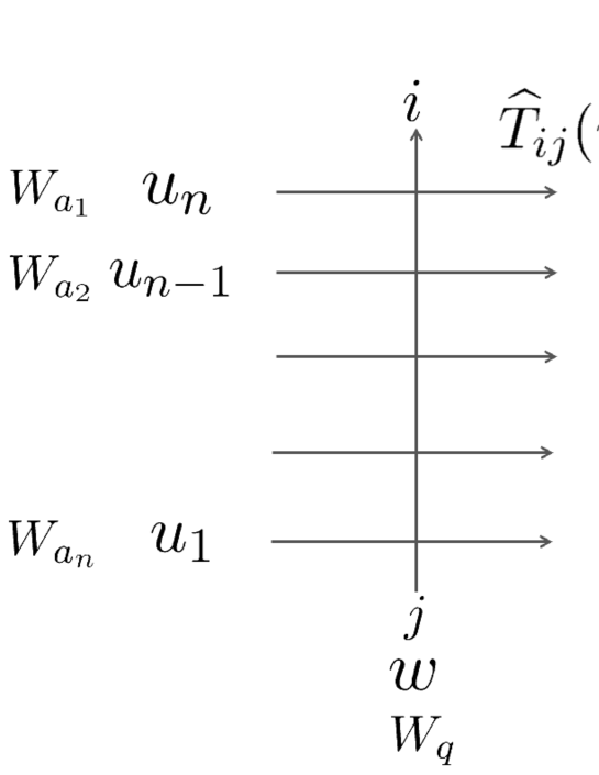
Figure 13: The matrix elements of the “vertical” monodromy matrix with respect to the quantum space $\widehat{T}_{ij}(w|u_{1},\dots,u_{n})$ (6.8).

From the observation above, we have the following formula for the $K$-theoretic Gysin map for example: Let $E\longrightarrow X$ be a rank $n$ complex vector bundle and $u_{1},\dots,u_{n}$ be Grothendieck roots of $E^{\vee}$. Let $H_{j}\longrightarrow X$ ($j=0,1,\dots,m$) be rank $h_{j}$ complex vector bundles with Grothendieck roots $w_{\sum_{k=0}^{j-1}h_{k}+1},w_{\sum_{k=0}^{j-1}h_{k}+2},\dots,w_{\sum_{k=0}^{j}h_{k}}$ ($h_{-1}:=0$). Take a positive integer $p$ satisfying $p\geq\sum_{k=0}^{m}h_{k}$. Let $\pi_{q_{1},\dots,q_{m}}$ be the partial flag bundle $\pi_{q_{1},\dots,q_{m}}:\mathcal{F\ell}_{q_{1},\dots,q_{m}}(E)\longrightarrow X$ . For ordered sets of integers $I$ and $J$ which have the following forms $I=(0^{h_{0}},1^{h_{1}},\dots,m^{h_{m}},i_{\sum_{k=0}^{m}h_{k}+1},\dots,i_{p})$ and $J=(0^{h_{0}},1^{h_{1}},\dots,m^{h_{m}},j_{\sum_{k=0}^{m}h_{k}+1},\dots,j_{p})$, the $K$-theoretic pushforward $\pi_{q_{1},\dots,q_{m}*}:K^{0}(\mathcal{F\ell}_{q_{1},\dots,q_{m}}(E))\longrightarrow K^{0}(X)$ of
$F_{IJ}(u_{1},\dots,u_{n}|w_{1},\dots,w_{\sum_{k=0}^{m}h_{k}},1^{p-\sum_{k=0}^{m}h_{k}})$ is given by

$$\pi_{q_{1},\dots,q_{m}*}(F_{IJ}(u_{1},\dots,u_{n}|w_{1},\dots,w_{\sum_{k=0}^{m}h_{k}},1^{p-\sum_{k=0}^{m}h_{k}}))$$

$$= G_{IJ}(u_{1},\dots,u_{n}|w_{1},\dots,w_{\sum_{k=0}^{m}h_{k}},1^{p-\sum_{k=0}^{m}h_{k}}).$$ (6.10)

The following special case of (6.10): $m=1$, $h_{1}=0$, $J=(0^{p})$ and $I=(i_{1},i_{2},\dots,i_{p})$ where $i_{k}=1$ for $k=\lambda_{n-q_{1}}+1,\lambda_{n-q_{1}-1}+2,\dots,\lambda_{1}+(n-q_{1})$ $(h_{0}+1\leq\lambda_{n-q_{1}}+1<\lambda_{n-q_{1}-1}+2<\cdots<\lambda_{1}+(n-q_{1})\leq p)$ and $i_{k}=0$ otherwise, which corresponds to the case of Grassmann bundles, can be written down using double Grassmannian Grothendieck polynomials as

$$\pi_{q_{1}*}(G_{(\lambda_{1},\dots,\lambda_{n-q_{1}})}(1-u_{q_{1}+1}^{-1},\dots,1-u_{n}^{-1}|1-w_{1},\dotsm 1-w_{h_{0}},0,\dots)$$

$$\times G_{p^{q_{1}}}(1-u_{1}^{-1},\dots,1-u_{q_{1}}^{-1}|1-w_{1},\dots,1-w_{h_{0}},0,\dots))$$

$$= G_{((p-n+q_{1})^{q_{1}},\lambda_{1},\dots,\lambda_{n-q_{1}})}(1-u_{1}^{-1},\dots,1-u_{n}^{-1}|1-w_{1},\dots,1-w_{h_{0}},0,\dots).$$ (6.11)

Here, $G_{\lambda}(z_{1},\dots,z_{n}|v_{1},\dots)$ are the double Grassmannian Grothendieck polynomials [37, 40, 41, 42, 43, 44, 45] which have the following determinant form

$$G_{\lambda}(z_{1},\dots,z_{n}|v_{1},\dots)=\frac{\mathrm{det}_{n}([z_{i}|\boldsymbol{v}]^{\lambda_{j}+n-j}(1-z_{i})^{j-1})}{\prod_{1\leq i<j\leq n}(z_{i}-z_{j})},$$ (6.12)

where $\lambda=(\lambda_{1},\lambda_{2},\dots,\lambda_{n})$ is a partition, $\{z_{1},\dots,z_{n}\}$ and $\boldsymbol{v}=\{v_{1},\dots\}$ are sets of variables and

$$[z_{i}|\boldsymbol{v}]^{j}=(z_{i}\oplus v_{1})(z_{i}\oplus v_{2})\cdots(z_{i}\oplus v_{j}),$$ (6.13)

where $z\oplus v:=z+v-zv$.

One can show (6.11) by slightly extending the argument given in [35] as follows. First recall the following correspondence between partition functions of the five-vertex models and Grothendieck polynomials. We consider two types of partition functions

$$\langle I|\prod_{j=1}^{n}B_{0}(u_{j}|w_{1},\dots,w_{p})|0^{p}\rangle,$$ (6.14)

and

$$\langle I|\prod_{j=1}^{m}D_{1}(u_{j}|w_{1},\dots,w_{p})\prod_{j=1}^{n}B_{0}(u_{j+m}|w_{1},\dots,w_{p})|0^{p}\rangle,$$ (6.15)

where $I=(i_{1},i_{2},\dots,i_{p})$ is $i_{k}=1$ for $k=\lambda_{n}+1,\lambda_{n-1}+2,\dots,\lambda_{1}+n$ $(1\leq\lambda_{n}+1<\lambda_{n-1}+2<\cdots<\lambda_{1}+n\leq p)$ and $i_{k}=0$ otherwise. The first type of partition functions consisting of $B_{0}$-operators are represented by Grothendieck polynomials [10, 11, 26, 27, 43]

$$\langle I|\prod_{j=1}^{n}B_{0}(u_{j}|w_{1},\dots,w_{p})|0^{p}\rangle$$

$$= G_{(\lambda_{1},\dots,\lambda_{n})}(1-u_{1}^{-1},\dots,1-u_{n}^{-1}|1-w_{1},\dots,1-w_{p},0,\dots).$$ (6.16)

Next, note that Lemma 3.11 can be extended to inhomogeneous version as well, and we have the following equality

$$\langle I|\prod_{j=1}^{m}D_{1}(u_{j}|w_{1},\dots,w_{p})\prod_{j=1}^{n}B_{0}(u_{j+m}|w_{1},\dots,w_{p})|0^{p}\rangle$$

$$=\langle\{I,1^{m}\}|\prod_{j=1}^{m+n}B_{0}^{(p,m)}(u_{j}|w_{1},\dots,w_{p},1^{m})|0^{p+m}\rangle,$$ (6.17)

where

$$B_{0}^{(p,m)}(u|w_{1},\dots,w_{p},1^{m})={}_{a}\langle 0|R_{a,p+m}(u,1)\cdots R_{a,p+1}(u,1)R_{a,p}(u,w_{p})\cdots R_{a1}(u,w_{1})|1\rangle_{a}.$$ (6.18)

Combining (6.16) and (6.17) gives the following expression for the second type of partition functions

$$\langle I|\prod_{j=1}^{m}D_{1}(u_{j}|w_{1},\dots,w_{p})\prod_{j=1}^{n}B_{0}(u_{j+m}|w_{1},\dots,w_{p})|0^{p}\rangle$$

$$=G_{((p-n)^{m},\lambda_{1},\dots,\lambda_{n})}(1-u_{1}^{-1},\dots,1-u_{m+n}^{-1}|1-w_{1},\dots,1-w_{p},0,\dots).$$ (6.19)

We examine $F_{IJ}(u_{1},u_{2},\dots,u_{n}|w_{1},\dots,w_{h_{0}},1^{p-h_{0}})$ and $G_{IJ}(u_{1},u_{2},\dots,u_{n}|w_{1},\dots,w_{h_{0}},1^{p-h_{0}})$ where $J=(0^{p})$. First let us see

$$F_{IJ}(u_{1},u_{2},\dots,u_{n}|w_{1},\dots,w_{h_{0}},1^{p-h_{0}})$$

$$= \langle I|\prod_{j=q_{1}+1}^{n}B_{0}(u_{j}|w_{1},\dots,w_{h_{0}},1^{p-h_{0}})\prod_{j=1}^{q_{1}}D_{1}(u_{j}|w_{1},\dots,w_{h_{0}},1^{p-h_{0}})|0^{p}\rangle.$$ (6.20)

Using the action of the $D_{1}$-operators on $|0^{p}\rangle$

$$D_{1}(u|w_{1},\dots,w_{p})|0^{p}\rangle=\prod_{k=1}^{p}(1-w_{k}/u)|0^{p}\rangle,$$ (6.21)

we have

$$\prod_{j=1}^{q_{1}}D_{1}(u_{j}|w_{1},\dots,w_{h_{0}},1^{p-h_{0}})|0^{p}\rangle$$

$$=\prod_{j=1}^{q_{1}}\prod_{k=1}^{h_{0}}(1-w_{k}/u_{j})\prod_{j=1}^{q_{1}}\prod_{k=h_{0}+1}^{p}(1-1/u_{j})|0^{p}\rangle$$

$$=G_{p^{q_{1}}}(1-u_{1}^{-1},\dots,1-u_{q_{1}}^{-1}|1-w_{1},\dots,1-w_{h_{0}},0,\dots)|0^{p}\rangle,$$ (6.22)

(6.20) becomes

$$F_{IJ}(u_{1},u_{2},\dots,u_{n}|w_{1},\dots,w_{h_{0}},1^{p-h_{0}})$$

$$= G_{p^{q_{1}}}(1-u_{1}^{-1},\dots,1-u_{q_{1}}^{-1}|1-w_{1},\dots,1-w_{h_{0}},0,\dots)\langle I|\prod_{j=q_{1}+1}^{n}B_{0}(u_{j}|w_{1},\dots,w_{h_{0}},1^{p-h_{0}})|0^{p}\rangle.$$ (6.23)

Applying the correspondence (6.16) to the right hand side of (6.23) (recall the sequence $I$ what we consider in (6.23) is the following: $I=(i_{1},i_{2},\dots,i_{p})$ where $i_{k}=1$ for $k=\lambda_{n-q_{1}}+1,\lambda_{n-q_{1}-1}+2,\dots,\lambda_{1}+(n-q_{1})$ $(h_{0}+1\leq\lambda_{n-q_{1}}+1<\lambda_{n-q_{1}-1}+2<\cdots<\lambda_{1}+(n-q_{1})\leq p)$ and $i_{k}=0$ otherwise), we get

$$F_{IJ}(u_{1},u_{2},\dots,u_{n}|w_{1},\dots,w_{h_{0}},1^{p-h_{0}})$$

$$= G_{(\lambda_{1},\dots,\lambda_{n-q_{1}})}(1-u_{q_{1}+1}^{-1},\dots,1-u_{n}^{-1}|1-w_{1},\dotsm 1-w_{h_{0}},0,\dots)$$

$$\times G_{p^{q_{1}}}(1-u_{1}^{-1},\dots,1-u_{q_{1}}^{-1}|1-w_{1},\dots,1-w_{h_{0}},0,\dots).$$ (6.24)

Next we examine $G_{IJ}(u_{1},u_{2},\dots,u_{n}|w_{1},\dots,w_{h_{0}},1^{p-h_{0}})$

$$G_{IJ}(u_{1},u_{2},\dots,u_{n}|w_{1},\dots,w_{h_{0}},1^{p-h_{0}})$$

$$= \langle I|\prod_{j=1}^{q_{1}}D_{1}(u_{j}|w_{1},\dots,w_{h_{0}},1^{p-h_{0}})\prod_{j=q_{1}+1}^{n}B_{0}(u_{j}|w_{1},\dots,w_{h_{0}},1^{p-h_{0}})|0^{p}\rangle.$$ (6.25)

Applying the correspondence (6.19) to the right hand side of (6.25) gives

$$G_{IJ}(u_{1},u_{2},\dots,u_{n}|w_{1},\dots,w_{h_{0}},1^{p-h_{0}})$$

$$= G_{((p-n+q_{1})^{q_{1}},\lambda_{1},\dots,\lambda_{n-q_{1}})}(1-u_{1}^{-1},\dots,1-u_{n}^{-1}|1-w_{1},\dots,1-w_{h_{0}},0,\dots).$$ (6.26)

(6.24) and (6.26) gives (6.11).

Finally we note (6.11) is also a special case of the following formula derived by Buch [37].

Theorem 6.1.

(Buch [37], Theorem 7.3) Let $\mathcal{A}\longrightarrow X$ and $\mathcal{B}\longrightarrow X$ be complex vector bundles of rank $n$ and $\ell$ respectively. Let $\pi:\mathrm{Gr}_{k}(\mathcal{A})\longrightarrow X$ be the Grassmann bundle of $k$-planes in $\mathcal{A}$ with universal tautological exact sequence $0\rightarrow\mathcal{S}\rightarrow\pi^{*}\mathcal{A}\rightarrow\mathcal{Q}\rightarrow 0$ of vector bundles over $\mathrm{Gr}_{k}(\mathcal{A})$. Let $\{\alpha_{1},\dots,\alpha_{n}\}$, $\{\beta_{1},\dots,\beta_{\ell}\}$, $\{\sigma_{1},\dots,\sigma_{k}\}$ and $\{\omega_{1},\dots,\omega_{n-k}\}$ be the sets of Grothendieck roots for bundles $\mathcal{A}$, $\mathcal{B}$, $\mathcal{S}$ and $\mathcal{Q}$ respectively. Let $I=(I_{1},\dots,I_{n-k})$ and $J=(J_{1},J_{2},\dots)$ be sequences of integers satisfying $I_{j}\geq\ell$ for all $j$. Then we have

$$\pi_{*}(G_{I}(\mathcal{Q}-\mathcal{B})G_{J}(\mathcal{S}-\mathcal{B}))=G_{I-(k)^{n-k},J}(\mathcal{A}-\mathcal{B}).$$ (6.27)

Here, $G_{I}(\mathcal{A}-\mathcal{B})$ in (6.27) are certain Grothendieck classes of $K^{0}(X)$ extended to sequences of integers [37] from the case when $I$ are partitions $I=\lambda=(\lambda_{1},\dots,\lambda_{i})$ satisfying $n\geq i$, in which case $G_{\lambda}(\mathcal{A}-\mathcal{B})$ are the Grassmannian double Grothendieck polynomials

$$G_{\lambda}(\mathcal{A}-\mathcal{B})=G_{\lambda}(1-\alpha_{1}^{-1},\dots,1-\alpha_{n}^{-1}|1-\beta_{1},\dots,1-\beta_{\ell}).$$ (6.28)

To compare (6.11) with Theorem 6.1, let us first recall that (6.11) is the pushforward from the Grothendieck group of $\mathcal{F\ell}_{q_{1}}(E)$. There is an isomorphism $\mathrm{Gr}_{n-q_{m}}(E/U_{q_{m}})\simeq\mathcal{F\ell}_{q_{1},\dots,q_{m}}(E)$ between Grassmann bundles and partial flag bundles. See [111] Remark 3.3 for example. We also use this to match with the former result for Grassmann bundles [35]. Using this isomorphism, we identify bundles $\mathcal{A}$, $\mathcal{S}$ and $\mathcal{Q}$ in Thm 6.1 with bundles $E^{\vee}$, $(E/U_{q_{1}})^{\vee}$ and $U_{q_{1}}^{\vee}$, respectively. We also identify $\mathcal{B}$ with $H_{0}$. Under these identifications, (6.11) can be written as

$$\pi_{*}(G_{p^{\mathrm{rank}(\mathcal{Q})}}(\mathcal{Q}-\mathcal{B})G_{\lambda}(\mathcal{S}-\mathcal{B}))=G_{((p-\mathrm{rank}(\mathcal{S}))^{\mathrm{rank}(\mathcal{Q})},\lambda)}(\mathcal{A}-\mathcal{B}),$$ (6.29)

where $p\geq h_{0}=\mathrm{rank}(\mathcal{B})$. One can see this corresponds to the case $J=\lambda$, $I_{1}=\cdots=I_{n-k}\geq\ell$ of Theorem 6.1.

References

• [1] H. Bethe, Z. Phys. 71, 205 (1931).
• [2] E. H. Lieb and F.Y.Wu, Two-dimensional ferroelectric models, in Phase Transitions and Critical Phenomena (Academic Press, London, 1972), Vol. 1, pp. 331-490.
• [3] R.J. Baxter, Exactly Solved Models in Statistical Mechanics (Academic Press, London, 1982).
• [4] V.E. Korepin, N.M. Bogoliubov and A.G. Izergin, Quantum Inverse Scattering Method and Correlation functions (Cambridge University Press, Cambridge, 1993).
• [5] V. Drinfeld, Sov. Math. Dokl. 32, 254 (1985).
• [6] M. Jimbo, Lett. Math. Phys. 10, 63 (1985).
• [7] L. D. Faddeev, E. K. Sklyanin and L. A. Takhtajan, Theor. Math. Phys. 40, 194 (1979).
• [8] P. P. Kulish, N. Yu. Reshetikhin and E. K. Sklyanin, Lett. Math. Phys. 5, 393 (1981).
• [9] V. Gorbounov, R. Rimรกnyi, V. Tarasov and A. Varchenko, J. Geom. Phys. 74, 56 (2013).
• [10] K. Motegi and K. Sakai, J. Phys. A: Math. Theor. 46, 355201 (2013).
• [11] K. Motegi, K. and Sakai, J. Phys. A: Math. Theor. 47, 445202 (2014).
• [12] R. Rimรกnyi, V. Tarasov and A. Varchenko, J. Geom. Phys. 94, 81 (2015).
• [13] M. Aganagic and A. Okounkov, Moscow Math. J. 17, 565 (2017).
• [14] A. Okounkov, Lectures on $K$-theoretic computations in enumerative geometry, In: Geometry of Moduli Spaces and Representation Theory, IAS/Park City Math. Ser., 24, Amer. Math. Soc., Providence, RI, (2017), pp. 251-380.
• [15] D. Maulik and A. Okounkov, Quantum groups and quantum cohomology, Astรฉrisque, 408 (2019).
• [16] M. Aganagic and A. Okounkov, J. Amer. Math. Soc. 34, 79 (2021).
• [17] G. Felder, R. Rimรกnyi and A. Varchenko, SIGMA 14, 132 (2018).
• [18] H. Konno, J. Int. Syst. 2, xyx011 (2017).
• [19] H. Konno, J. Int. Syst. 3, xyy012 (2018).
• [20] T. Ikeda, S. Iwao and T. Maeno, Int. Math. Res. Not. 19, 6421 (2020).
• [21] P.P. Pushkar, A. Smirnov and A.M. Zeitlin, Adv. Math. 360, 106919 (2020).
• [22] P. Koroteev, P.P. Pushkar, A. Smirnov and A.M. Zeitlin, Sel. Math. New Ser. 27, 87 (2021).
• [23] P. Koroteev and A.M. Zeitlin, Math.Res.Lett. 28, 435 (2021).
• [24] A. Smirnov and A. Okounkov, Invent. math. 229, 1203 (2022).
• [25] A.N. Kirillov, SIGMA 12, 034 (2016).
• [26] V. Gorbounov and C. Korff, Adv. Math. 313, 282 (2017).
• [27] M. Wheeler and P. Zinn-Justin, J. Reine Angew. Math. 757, 159 (2019).
• [28] V. Buciumas and T. Scrimshaw, Int. Math. Res. Not. 10, 7231 (2022).
• [29] B. Brubaker, C. Frechette, A. Hardt, E. Tibor and K. Weber, Frozen Pipes: Lattice Models for Grothendieck Polynomials, arXiv:2007.04310.
• [30] P. Zinn-Justin, SIGMA 14 paper 69, 48 (2018).
• [31] D. Yeliussizov, J. Comb. Th. A 161, 453 (2019).
• [32] S. Iwao, Alg. Comb. 3, 1023 (2020).
• [33] S. Iwao, J. Alg. Comb. 56, 493 (2022).
• [34] S. Iwao, Free fermions and Schur expansions of multi-Schur functions, arXiv:2105.02604.
• [35] K. Motegi, Nucl. Phys. B, 971, 115513 (2021).
• [36] W. Gu, L. Mihalcea, E. Sharpe and H. Zou J. Geom. Phys. 177, 104548 (2022).
• [37] A.S. Buch, Duke Math. J. 115, 75 (2002).
• [38] P. Pragacz, Ann. Sci. ร‰cole Norm. Sup. 21, 413 (1988).
• [39] W. Fulton and P. Pragacz, Schubert varieties and degeneracy loci, (Springer-Verlag, Berlin, 1998) Appendix J by the authors in collaboration with I. Ciocan-Fontanine.
• [40] A. Lascoux and M. Schรผtzenberger, Structure de Hopf de lโ€™anneau de cohomologie et de lโ€™anneau de Grothendieck dโ€™une variรฉtรฉ de drapeaux, C. R. Acad. Sci. Parix Sรฉr. I Math 295 (1982) 629.
• [41] S. Fomin and A.N. Kirillov, Grothendieck polynomials and the Yang-Baxter equation, Proc. 6th Internat. Conf. on Formal Power Series and Algebraic Combinatorics, DIMACS (1994) 183-190.
• [42] P.J. McNamara, Electron. J. Combin. 13, 71 (2006).
• [43] T. Ikeda and H. Naruse, Adv. Math. 243, 22 (2013).
• [44] A.S. Buch, Acta. Math. 189, 37 (2002).
• [45] A.S. Buch, Combinatorial $K$-theory, Topics in cohomological studies of algebraic varieties, Trends Math., Birkhรคuser, Basel, 2005, pp. 87-103.
• [46] A.S. Buch, Michigan Math. J. 57, 93 (2008).
• [47] A.S. Buch, L.C. Mihalcea, Duke Math. J. 156, 501 (2011).
• [48] C. Lenart, Ann. Comb. 4, 67 (2000).
• [49] V.E. Korepin, Comm. Math. Phys. 86, 391 (1982).
• [50] A. Izergin, Sov. phys. Dokl. 32, 878 (1987).
• [51] G. Kuperberg, Int. Math. Res. Not. 3, 139 (1996).
• [52] O. Tsuchiya, J. Math. Phys. 39, 5946 (1998).
• [53] S. Pakuliak, V. Rubtsov and A. Silantyev, J. Phys. A: Math. and Theor. 41, 295204 (2008).
• [54] H. Rosengren, Adv. Appl. Math. 43, 137 (2009).
• [55] M. Wheeler, Nucl. Phys. B 852, 468 (2011).
• [56] K. Motegi, J. Math. Phys. 59, 053505 (2018).
• [57] A. Hamel and R.C. King, J. Alg. Comb. 16, 269 (2002).
• [58] N. M. Bogoliubov, J. Phys. A: Math. and Gen. 38, 9415 (2005).
• [59] K. Shigechi and M. Uchiyama, J. Phys. A: Math. Gen. 38, 10287 (2005).
• [60] B. Brubaker, D. Bump and S. Friedberg, Comm. Math. Phys. 308, 281 (2011).
• [61] D. Bump, P. McNamara and M. Nakasuji, Comm. Math. Univ. Sancti Pauli. 63, 23 (2014).
• [62] A. Lascoux, SIGMA 3, 029 (2007).
• [63] P.J. McNamara, Factorial Schur functions via the six-vertex model, arXiv:0910.5288.
• [64] C. Korff and C. Stroppel, Adv. Math. 225, 200 (2010).
• [65] C. Korff, Lett. Math. Phys. 104, 771 (2014).
• [66] D. Betea and M. Wheeler, J. Comb. Theory, Series A. 137, 126 (2016).
• [67] D. Betea, M. Wheeler and P. Zinn-Justin, J. Alg. Comb. 42, 555 (2015).
• [68] M. Wheeler and P. Zinn-Justin, Adv. Math. 299, 543 (2016).
• [69] A. Borodin, Adv. Math. 306, 973 (2017).
• [70] A. Borodin and L. Petrov, Sel. Math. New Ser. 24, 751 (2018).
• [71] Y. Takeyama, Funkcialaj Ekvacioj 61, 349 (2018).
• [72] J.F. van Diejen and E. Emsiz, Comm. Math. Phys. 350, 1017 (2017).
• [73] B. Brubaker, V. Buciumas and D. Bump, Communications in Number Theory and Physics. 13, 101 (2019).
• [74] B. Brubaker, V. Buciumas, D. Bump and N. Gray, Appendix to [73].
• [75] B. Brubaker, V. Buciumas, D. Bump and H.P.A. Gustafsson, J. Comb. Th. Series A, 178, 105354 (2021).
• [76] A. Borodin and M. Wheeler, Coloured stochastic vertex models and their spectral theory, arXiv:1808.01866.
• [77] C. Zhong, Lett. Math. Phys. 112, 55 (2022).
• [78] O. Foda and M. Manabe, J. High Energ. Phys. 2019, 36 (2019).
• [79] K. Motegi, J. Math. Phys. 61, 053507 (2020).
• [80] A. Aggarwal, A. Borodin and M. Wheeler, Colored Fermionic Vertex Models and Symmetric Functions, arXiv:2101.01605.
• [81] B. Brubaker, V. Buciumas, D. Bump and H.P.A. Gustafsson, Metaplectic Iwahori Whittaker functions and supersymmetric lattice models, arXiv:2012.15778.
• [82] K. Motegi, Nucl. Phys. B 954, 114998 (2020).
• [83] L.M. Fehรฉr, A. Nรฉmethi and R. Rimรกnyi, Comment. Math. Helv. 87, 861 (2012).
• [84] P.L. Guo and S.C.C. Sun, Adv. App. Math. 111, 101933 (2019).
• [85] J. Allman, $K$-classes of quiver cycles, Grothendieck polynomials, and iterated residues, PhD thesis, UNC-Chapel Hill, 2014,
• [86] J. Allman, Michigan Math. J. 63, 865 (2014).
• [87] M. Atiyah and R. Bott, Topology 23, 1 (1984).
• [88] N. Berline and M. Vergne, C. R. Acad. Sci. Paris, 295, 539 (1982).
• [89] N. Chriss and V. Ginzburg, Representation Theory and Complex Geometry. Modern Birkhรคuser Classics. Birkhรคuser Boston, 2009.
• [90] H. A. Nielsen, Bull. Soc. Math. France, 102, 97 (1974).
• [91] A. Grothendieck, Formule de Lefschetz, (Rรฉdigรฉ par L. Illusie). In Sรฉminaire de gรฉomรฉtrie algรฉbrique du Bois-Marie 1965-66, SGA 5, Lect. Notes Math. 589, Exposรฉ No.III., pages 73-137. 1977.
• [92] P. Baum, W. Fulton, and G. Quart, Acta Math. 143, 193 (1979).
• [93] P. Bressler and S. Evens, Trans. Amer. Math. Soc. 317, 799 (1990).
• [94] P. Pragacz, Algebro-Geometric applications of Schur $S$- and $Q$-polynomials, Topics in invariant theory (Springer, Berlin, 1991) (Paris, 1989/1990), 130-191, Lecture Notes in Math., 1478.
• [95] P. Pragacz, Symmetric polynomials and divided differences in formulas of intersection theory, Parameter Spaces (P. Pragacz, ed.), 36, Banach Center Publications, 125 (1996).
• [96] L. Tu, Computing the Gysin map using fixed points, arXiv:1507.00283.
• [97] A. Weber and M. Zielenkiewicz, J. Alg. Comb. 49, 361 (2019).
• [98] R. Rimรกnyi, J. Alg. Comb. 40, 527 (2014).
• [99] J. Allman and R. Rimรกnyi, An iterated residue perspective on stable Grothendieck polynomials, arXiv:1408.1911.
• [100] J. Allman and R. Rimรกnyi, $K$-theoretic Pieri rule via iterated residues, Sรฉminaire Lotharingien de Combinatoire 80B (2018) Article 48.
• [101] R. Rimรกnyi and A. Szenes, Residues, Grothendieck polynomials and $K$-theoretic Thom polynomials, arXiv:1811.02055.
• [102] M. Zielenkiewicz, Centr. Eur. J. Math. 12, 574 (2014).
• [103] M. Zielenkiewicz, J. Symp. Geom. 16, 1455 (2018).
• [104] M. Zielenkiewicz, The Gysin homomorphism for homogeneous spaces via residues, PhD Thesis, University of Warsaw, arXiv:1702.04123, 2017.
• [105] P. Pragacz, Proc. Amer. Math. Soc. 143, 4705 (2015).
• [106] L. Darondeau and P. Pragacz, Int. J. Math. 28, 1750077 (2017).
• [107] L. Darondeau and P. Pragacz, Fundamenta Mathematicae 244, 191 (2019).
• [108] T. Hudson, T. Ikeda, T. Matsumura and H. Naruse, Adv. Math. 320, 115 (2017).
• [109] M. Nakagawa and H. Naruse, Contemp. Math. 708, 201 (2018).
• [110] M. Nakagawa and H. Naruse, Generating functions for the universal Hall-Littlewood $P$- and $Q$-functions, arXiv:1705.04791.
• [111] M. Nakagawa and H. Naruse, Math. Ann. 381, 335 (2021).