Theory of Optical Activity in Doped Systems with Application to Twisted Bilayer Graphene

Abstract

We theoretically study the optical activity in a doped system and derive the optical activity tensor from a light wavevector-dependent linear optical conductivity. Although the light-matter interaction is introduced through the velocity gauge from a minimal coupling Hamiltonian, we find that the well-known “false divergences” problem can be avoided in practice if the electronic states are described by a finite band effective Hamiltonian, such as a few-band tight-binding model. The expression we obtain for the optical activity tensor is in good numerical agreement with a recent theory derived for an undoped topologically trivial gapped system. We apply our theory to the optical activity of a gated twisted bilayer graphene, with a detailed discussion of the dependence of the results on twist angle, chemical potential, gate voltage, and location of rotation center forming the twisted bilayer graphene.

I Introduction

Optical activity, also known as optical rotatory power, describes the rotation of the polarization direction as light propagates through an optically active medium [1, 2]. This phenomenon arises from the different responses to left and right circularly polarized light; the difference in absorption of the two polarizations is referred to as circular dichroism [3].

Despite the broad application of circular dichroism in detecting the chirality of molecules [4, 5], the relevant research in crystals is limited [6, 7]. The quantum treatment of optical activity tensor is usually obtained from the charge-current density response [1, 8, 9, 10] with the light-matter interaction included via the minimal coupling Hamiltonian [9]. However, this method can lead to “false divergences” when the set of bands involved in the calculation is inevitably truncated [11, 12], and appropriate “sum rules” must be applied to show that the prefactors multiplying the divergent terms in fact vanish. To avoid this difficulty in calculating the optical activity, Mahon and Sipe [1] proposed a multipole moment expansion method for optical conductivity, where the macroscopic fields are introduced through the interactions with electric dipole, magnetic dipole, and electric quadrupole moments associated with Wannier functions at the lattice sites. Despite the link this approach identifies with treating the optical response of isolated molecules, the derivation is complicated and the treatment is at present limited to undoped, topologically trivial insulators.

Alternate derivations — particularly if they are simpler — can often stimulate new research. Starting from a minimal coupling Hamiltonian, in this paper we derive the expressions for the optical activity from the linear conductivity tensor at finite light wavevector. We then apply this method to study the optical activity of twisted bilayer graphene (TBG) using a simple tight-binding model [13, 14, 15] to describe its electronic states. The optical response of TBG has been extensively studied [16, 17, 18, 19], with the optical activity of undoped TBG investigated both experimentally [20] and theoretically [13]. In the undoped limit we find agreement with the results of Mahon and Sipe [1], except for an extra term that indeed seems to exhibit a “false divergence”; however, while we cannot confirm analytically that the prefactor of this term vanishes, we can verify that it has a negligible value in our finite band tight-binding model. And our approach is more general than that of Mahon and Sipe [1] in that it can be extended to doped systems; as well, it does not explicitly involve Wannier functions and the topological considerations necessary to construct them as localized functions. With our results in hand, we explore the dependence of the optical activity tensor on twist angle, chemical potential, gate voltage, and location of rotation center forming twisted bilayer graphene.

II Models

II.1 Optical activity tensor

An optically active material has different responses to left and right circularly polarized light, which are described by its linear optical conductivity $\sigma^{da}(\bm{q},\omega)$. For an electric field ${\bm{E}}({\bm{r}},t)={\bm{E}}({\bm{q}},\omega)e^{i({\bm{q}}\cdot{\bm{r}}-\omega t)}+{\rm c.c.}$, the induced optical current is $\bm{J}(\bm{r},t)=\bm{J}(\bm{q},\omega)e^{i({\bm{q}}\cdot{\bm{r}}-\omega t)}+{\rm c.c.}$ with $J^{d}({\bm{q}},\omega)=\sigma^{da}({\bm{q}},\omega)E^{a}({\bm{q}},\omega)$. The Roman letters in the superscript denote Cartesian directions $x/y/z$, and the repeated superscripts are summed over. Without losing generality, considering an incident light propagating along the $z$-direction, the response to the circularly polarized light can be written as [21]

$$J^{\delta_{1}}(q\hat{\bm{z}},\omega)=\sigma^{\delta_{1}\delta_{2}}(q\hat{\bm{z}},\omega)E^{\delta_{2}}(q\hat{\bm{z}},\omega)\,,$$ (1)

where $J^{\delta}=(J^{x}+i\delta J^{y})/\sqrt{2}$ with $\delta=\pm$ gives the left ($+$)/right ($-$) circular component of the current; a similar definition applies to $E^{\delta}$. Then the diagonal response coefficients are

$$\sigma^{\delta\delta}(q\hat{\bm{z}},\omega) =\frac{\sigma^{xx}+\sigma^{yy}-i\delta(\sigma^{xy}-\sigma^{yx})}{2}\,.$$ (2)

For nonzero $\sigma^{xy}-\sigma^{yx}$, the responses to the left and right circularly polarized lights are not the same, and the circular dichroism can be characterized by the ellipticity spectra $\Psi=(\alpha_{+}-\alpha_{-})/(2(\alpha_{+}+\alpha_{-}))$, where $\alpha_{\delta}$ is the absorption of the $\delta$ circularly polarized light [22]. For two-dimensional materials, the absorption is proportional to $\text{Re}[\sigma^{\delta\delta}]$, and we can get

$$\Psi=\frac{\text{Im}[\sigma^{xy}-\sigma^{yx}]}{2\text{Re}[\sigma^{xx}+\sigma^{yy}]}\,.$$ (3)

The wave vector $\bm{q}$ appearing in the linear conductivity $\sigma^{da}(\bm{q},\omega)$ is very small compared to most electron wave vectors, and up to the first order in $\bm{q}$ the conductivity can be expanded as

$$\sigma^{da}({\bm{q}},\omega)=\sigma^{da}(\omega)+S^{dac}(\omega)q^{c}+\cdots\,,$$ (4)

with $\sigma^{da}(\omega)\equiv\sigma^{da}({\bm{0}},\omega)$ giving the long wavelength limit, and

$$\left.S^{dac}(\omega)\equiv\frac{\partial\sigma^{da}({\bm{q}},\omega)}{\partial q^{c}}\right|_{{\bm{q}}=0}\,.$$ (5)

The latter arises from effects of magnetic dipole and electric quadrupole, and modified electric dipole effects [21]. From macroscopic optics, it gives the response of the current to the spatial derivative of the electric field, including contributions following from Faraday’s law.

For non-magnetic materials, the conductivity tensor $\sigma^{da}(\omega)$ has either no off-diagonal components or equal off-diagonal components $\sigma^{da}(\omega)=\sigma^{ad}(\omega)$ [23], and the optical activity mainly comes from the terms involving $S^{dac}(\omega)$, which is our focus in this paper. Because $S^{dac}(\omega)$ is a third-order tensor, it is nonzero only for crystals breaking inversion symmetry; more specifically, the nonzero $\text{Im}[\sigma^{xy}-\sigma^{yx}]$ indicates a chiral structure.

II.2 A microscopic response theory for $S^{dac}(\omega)$

For very weak electromagnetic fields, the Hamiltonian with the inclusion of light-matter interaction is taken from the minimal coupling as

$$\hat{H}(t)= \hat{H}_{0}+\frac{-e}{2}\left[\hat{v}^{a}A^{a}({\bm{r}},t)+A^{a}({\bm{r}},t)\hat{v}^{a}\right]+\frac{(-e)^{2}}{4}\left[\hat{M}^{da}A^{d}({\bm{r}},t)A^{a}({\bm{r}},t)\right.$$

$$\left.+A^{d}({\bm{r}},t)A^{a}({\bm{r}},t)\hat{M}^{da}\right]+\cdots\,,$$ (6)

with the electronic charge $e$, $\hat{\bm{v}}^{a}=[\hat{r}^{a},\hat{H}_{0}]/(i\hbar)$, and $\hat{M}^{da}=[\hat{r}^{d},\hat{v}^{a}]/(i\hbar)$. Here $\hat{H}_{0}$ is the crystal Hamiltonian without external field, $\hat{v}^{a}$ is the velocity operator, $\hat{M}^{da}$ is an operator associated with the mass term, and $A^{a}(\hat{\bm{r}},t)$ is the $a$th component of the vector potential of the electromagnetic field. The detailed explanation of this Hamiltonian is listed in Appendix A. The field operator can be expanded as

$$\hat{\Psi}(\bm{r},t) =\sum_{n}\int d\bm{k}\hat{a}_{n\bm{k}}(t)\phi_{n\bm{k}}(\bm{r})\,.$$ (7)

Here $\phi_{n\bm{k}}(\bm{r})=1/\sqrt{(2\pi)^{3}}e^{i\bm{k}\cdot\bm{r}}u_{n\bm{k}}(\bm{r})$ are the band eigenstates of $\hat{H}_{0}$ with band eigenenergies $\varepsilon_{n\bm{k}}$ and periodic functions $u_{n\bm{k}}(\bm{r})$, and $\hat{a}_{n\bm{k}}(t)$ is an annihilation operator of this state. The second quantization form of the Hamiltonian $\hat{H}(t)$ is

$$\hat{H}(t)= \sum_{n}\int_{\text{BZ}}d\bm{k}\varepsilon_{n\bm{k}}\hat{a}_{n\bm{k}}^{\dagger}\hat{a}_{n\bm{k}}+\int\frac{d\bm{q}}{(2\pi)^{3}}(-e)A^{a}_{\bm{q}}(t)\sum_{nm}\int_{\text{BZ}}d\bm{k}{\cal V}_{n\bm{k}+\bm{q},m\bm{k}}^{(1);a}\hat{a}_{n\bm{k}+\bm{q}}^{\dagger}\hat{a}_{m\bm{k}}$$

$$+\frac{1}{2}\int\frac{d\bm{q}_{1}d\bm{q}_{2}}{(2\pi)^{6}}(-e)^{2}A^{a}_{\bm{q}_{1}}(t)A^{b}_{\bm{q}_{2}}(t)\sum_{nm}\int_{\text{BZ}}d\bm{k}{\cal V}_{n\bm{k}+\bm{q}_{1}+\bm{q}_{2},m\bm{k}}^{(2):ab}\hat{a}_{n\bm{k}+\bm{q}_{1}+\bm{q}_{2}}^{\dagger}\hat{a}_{m\bm{k}}\,.$$ (8)

Here $A^{a}_{\bm{q}}(t)=\int d\bm{r}A^{a}(\bm{r},t)e^{-i\bm{q}\cdot\bm{r}}$ is the Fourier component of the vector potential, and the matrix elements are given by

$${\cal V}^{(1);a}_{n\bm{k},m\bm{k}_{1}} =\frac{1}{2}\sum_{l}\left(v^{a}_{nl\bm{k}}{\cal U}_{l\bm{k},m\bm{k}_{1}}+{\cal U}_{n\bm{k},l\bm{k}_{1}}v^{a}_{lm\bm{k}_{1}}\right)\,,$$ (9)

$${\cal V}^{(2);ab}_{n\bm{k},m\bm{k}_{1}} =\frac{1}{2}\sum_{l}\left(M^{ab}_{nl\bm{k}}{\cal U}_{l\bm{k},m\bm{k}_{1}}+{\cal U}_{n\bm{k},l\bm{k}_{1}}M^{ab}_{lm\bm{k}_{1}}\right)\,,$$ (10)

$${\cal U}_{n\bm{k},m\bm{k}_{1}} =\int_{uc}\frac{d\bm{r}}{\Omega}u^{*}_{n\bm{k}}(\bm{r})u_{m\bm{k}_{1}}(\bm{r})\,,$$ (11)

where $v_{nm\bm{k}}^{a}$ and $M_{nm\bm{k}}^{ab}$ are the matrix elements of single particle operators $\hat{v}^{a}$ and $\hat{M}^{ab}$, respectively; $\Omega$ is the volume of the unit cell. The current density operator is given as

$$\hat{J}^{a}({\bm{q}},t)= \int d\bm{r}\hat{J}^{a}(\bm{r},t)e^{i\bm{q}\cdot\bm{r}}=-\int d\bm{r}\frac{\delta\hat{H}(t)}{\delta A^{a}(\bm{r},t)}e^{i\bm{q}\cdot\bm{r}}=-(2\pi)^{3}\frac{\delta\hat{H}(t)}{\delta A^{a}_{-\bm{q}}(t)}\,,$$ (12)

and the conductivity can be obtained from the Kubo formula as [24]

$$\sigma^{da}(\bm{q},\omega)= -g_{s}\frac{|e|^{2}}{i\omega}\sum_{nm}\int_{\text{BZ}}\frac{d\bm{k}}{(2\pi)^{3}}\frac{{\cal V}^{(1);d}_{m\bm{k},n\bm{k}+\bm{q}}{\cal V}_{n\bm{k}+\bm{q},m\bm{k}}^{(1);a}(f_{m\bm{k}}-f_{n\bm{k}+\bm{q}})}{\hbar\omega-(\varepsilon_{n\bm{k}+\bm{q}}-\varepsilon_{m\bm{k}})+i0^{+}}$$

$$-g_{s}\frac{|e|^{2}}{i\omega}\sum_{n}\int_{\text{BZ}}\frac{d\bm{k}}{(2\pi)^{3}}{\cal V}^{(2);da}_{n\bm{k},n\bm{k}}f_{n\bm{k}}\,,$$ (13)

where the prefactor $g_{s}$ is the spin degeneracy and $f_{mk}=\left[1+e^{(\varepsilon_{m\bm{k}}-\mu)/k_{B}T}\right]^{-1}$ gives the Fermi-Dirac distribution at the state $\phi_{m\bm{k}}(\bm{r})$ for a given temperature $T$ and chemical potential $\mu$. Furthermore, the optical activity tensor in Eq. (5) is obtained as

$$S^{dac}(\omega)= -g_{s}\frac{|e|^{2}}{2i\omega}\sum_{nm}\int_{\text{BZ}}\frac{d\bm{k}}{(2\pi)^{3}}\left\{\frac{iv_{mn\bm{k}}^{d}\{r_{\bm{k}}^{c},v_{\bm{k}}^{a}\}_{nm}-i\{r_{\bm{k}}^{c},v_{\bm{k}}^{d}\}_{mn}v_{nm\bm{k}}^{a}}{\hbar\omega^{+}-\hbar\omega_{nm\bm{k}}}f_{mn\bm{k}}\right.$$

$$\left.+\frac{v_{mn\bm{k}}^{d}v_{nm\bm{k}}^{a}}{\hbar\omega^{+}-\hbar\omega_{nm\bm{k}}}\left[\frac{\hbar(v_{nn\bm{k}}^{c}+v_{mm\bm{k}}^{c})f_{mn\bm{k}}}{\hbar\omega^{+}-\hbar\omega_{nm\bm{k}}}-\frac{\partial(f_{n\bm{k}}+f_{m\bm{k}})}{\partial k^{c}}\right]\right\}\,,$$ (14)

with $\hbar\omega^{+}=\hbar\omega+i0^{+}$, $\hbar\omega_{nm\bm{k}}=\varepsilon_{n\bm{k}}-\varepsilon_{m\bm{k}}$ and $f_{nm\bm{k}}=f_{n\bm{k}}-f_{m\bm{k}}$. Here, $\bm{r}_{nm\bm{k}}=(1-\delta_{nm})i\bm{\nabla}_{\bm{q}}U_{n\bm{k},m\bm{k}+\bm{q}}|_{\bm{q}=0}$ gives the off-diagonal terms of the Berry connection, which can be further calculated through $\bm{r}_{nm\bm{k}}=\bm{v}_{nm\bm{k}}/(i\omega_{nm\bm{k}})$. The detailed derivation is given in Appendix B.

II.3 Discussion of the expression Eq. (II.2)

When the light-matter interaction is described using the vector potential, sum rules can be required to remove the “false divergences” occurring at zero frequency [11, 12]. To address this, we first perform an analysis of the expression in Eq. (II.2) for the behavior as $\omega\to 0$. Utilizing

$$\frac{1}{\omega^{+}-\omega_{nm\bm{k}}}= -\frac{1}{\omega_{nm\bm{k}}}-\frac{\omega^{+}}{(\omega_{nm\bm{k}})^{2}}+\frac{({\omega^{+}})^{2}}{(\omega_{nm\bm{k}})^{2}(\omega^{+}-\omega_{nm\bm{k}})}\,,$$ (15a)

$$\frac{1}{(\omega^{+}-\omega_{nm\bm{k}})^{2}}= \frac{1}{\omega_{nm\bm{k}}^{2}}+\frac{2\omega^{+}}{(\omega_{nm\bm{k}})^{3}}+\frac{(3\omega_{nm\bm{k}}-2\omega^{+}){(\omega^{+})}^{2}}{(\omega_{nm\bm{k}})^{3}(\omega^{+}-\omega_{nm\bm{k}})^{2}}\,,$$ (15b)

the expression of $S^{dab}(\omega)$ is reorganized as

$$S^{dac}(\omega)=S_{f}^{dac}(\omega)+\frac{S_{-1}^{dac}}{\hbar\omega}+S_{0}^{dac}+S_{r}^{dac}(\omega)\,.$$ (16)

Here $S_{f}^{dac}(\omega)$ is the term involving derivatives of the populations; $S_{-1}^{dac}$ and $S_{0}^{dac}$ are independent of $\omega$, they come from the first two terms of Eqs. (15), respectively; $S_{r}^{dac}(\omega)$ collects all the remaining terms. Their expressions are given in Appendix C.

For an insulator, the term $S_{f}^{dac}(\omega)$ vanishes, while $S_{r}^{dac}(\omega)$ is at least proportional to $\omega$, and is exactly the same as the optical activity tensor derived by Mahon and Sipe [1]. The term $S_{0}^{dac}$ vanishes for a system with time reversal symmetry, as we show in Appendix C. Thus for a topologically trivial insulator the only difference between our result and that of Mahon and Sipe [1] is the term involving $S_{-1}^{dac}$. It leads to an $\omega^{-1}$ dependence in the conductivity, and for a cold clean insulator, a nonzero $S_{-1}^{dac}$ would lead to a divergent response as $\omega\to 0$, which is unphysical; and thus a zero value of $S_{-1}^{dac}$ is required in this case. Adopting a nonzero value for $S_{-1}^{dac}$ would lead to a “false divergence” in the optical activity tensor, similar to those that arise in calculations of the linear susceptibility [11, 12]; as is the situation there, the vanishing of $S_{-1}^{dac}$ should be confirmed by the use of sum rules. Though we have not found an analytic proof that $S_{-1}^{dac}$ vanishes, as it must if our results are both to agree with Mahon and Sipe [1] for a cold, clean, topologically trivial insulator, and indeed to be physically meaningful for such a system as $\omega\rightarrow 0$, we do numerically verify its value is negligible as long as a proper model Hamiltonian is adopted, as shown in the next section.

Compared to the approach of Mahon and Sipe [1], ours has several advantages: (1) Since it does not rely on a Wannier function basis, and the topological considerations that must be invoked to identify when localized Wannier functions can be introduced, it should be free of any assumptions on the topology of the band structure. (2) The contributions from free carriers are included. (3) Even beyond the small wavevector approximation — for example, when the material interacts with confined light in nanostructures — our expression in Eq. (13) can still be applied. For a model Hamiltonian composed of finite numbers of bands, the correct use of this expression for a numerical calculation requires the inclusion of all bands inside the model Hamiltonian and the integration over the whole Brillouin zone (BZ). Therefore, the direct application of the ab initio calculation is not suitable, while the combination with Wannier90 package [25] could provide a finite band Hamiltonian.

III Results

We apply the theory developed above to commensurate TBG, with the electronic states described by tight-binding models, as listed in Appendix D. To use the expressions for a two dimensional structure, the integration $\int_{\text{BZ}}\frac{d\bm{k}}{(2\pi)^{3}}$ should be replaced by $\int_{\text{BZ}}\frac{d\bm{k}}{(2\pi)^{2}}$ with a two dimensional $\bm{k}$. A TBG can be identified by the quantities $(m,n,\Delta,V_{g},\bm{\delta})$: the integer pairs $(m,n)$ are utilized to indicate the supercell and the twist angle $\theta$ [26, 16]; $\Delta$ represents the on-site energy differences between A and B sites which can be induced by asymmetric substrate effects [27, 28]; $V_{g}$ describes the potential differences between layers, which can be tuned by the gate voltage [29, 30]; and $\bm{\delta}$ describes the position of the rotation center, either at one carbon atom (for $\bm{\delta}=\bm{0}$) or at the center of one hexagon (for $\bm{\delta}=\bm{\delta}_{c}\equiv 2(\bm{a}_{1}+\bm{a}_{2})/3$).

In this work, we are interested in the TBGs with integer pairs $(m,n)=$ (2,1), (3,2), (4,3), (5,4), (6,5), (7,6), which correspond to twist angles of $21.8^{\circ}$, $13.2^{\circ}$, $9.4^{\circ}$, $7.3^{\circ}$, $6.0^{\circ}$, and $5.1^{\circ}$, respectively. For numerically evaluating the expressions in Eq. (II.2), the BZ is divided into a uniform grid of 1000 $\times$ 1000 for $(m,n)=$ (2,1), (3,2), (4,3), (5,4) and 500 $\times$ 500 for $(m,n)=$(6,5), (7,6), the temperature is taken as zero, and to avoid the divergences all frequencies $\omega$ are broadened as $\omega+i\gamma$ by a phenomenological parameter $\gamma$ with $\hbar\gamma=10$ meV, unless otherwise specified. The derivative of the population is converted to

$$\frac{\partial f_{n\bm{k}}}{\partial k^{a}} =-\hbar v_{nn\bm{k}}^{a}\frac{\partial f_{n\bm{k}}}{\partial\mu}\,,$$ (17)

and ${\partial f_{n\bm{k}}}/{\partial\mu}$ is numerically calculated by a difference between chemical potentials $\mu+\delta\mu/2$ and $\mu-\delta\mu/2$ with $\delta\mu=5$ meV.

Before presenting numerical results, we perform a symmetry analysis on the tensor components. The crystal symmetry depends on the values of $V_{g}$ and $\bm{\delta}$. For $V_{g}=0$, the point group is $D_{6}$ for $\bm{\delta}=\bm{\delta}_{c}$ and $D_{3}$ for $\bm{\delta}=\bm{0}$, and they are reduced to $C_{6}$ and $C_{3}$ for nonzero $V_{g}$, respectively. The nonzero components of the optical activity tensor are summarized in Table 1, and all cases include the tensor components $xyz=-yxz$, $xzy=-yzx$ and $zxy=-zyx$. Considering the geometry discussed in Section II.1, we mainly focused on the component $S^{xyz}$.

Table 1: Nonzero components of the optical activity tensor for different parameters [23].

TBG Parameters	Point Group	Nonzero Tensor Components
$(m,n,0,0,\bm{0})$	$D_{3}$	$xxx=-xyy=-yyx=-yxy$, $xyz=-yxz$,
		$xzy=-yzx$, $zxy=-zyx$
$(m,n,0,V_{g},\bm{0})$	$C_{3}$	$xxx=-xyy=-yyz=-yxy$, $xyz=-yxz$,
		$xzy=-yzx$, $zxy=-zyx$, $xzx=yzy$, $xxz=yyz$,
		$zxx=zyy$, $yyy=-yxx=-xxy=-xyx$, $zzz$
$(m,n,0,0,\bm{\delta}_{c})$	$D_{6}$	$xyz=-yxz$, $xzy=-yzx$, $zxy=-zyx$
$(m,n,0,V_{g},\bm{\delta}_{c})$	$C_{6}$	$xyz=-yxz$, $xzy=-yzx$, $zxy=-zyx$,
		$xzx=yzy$, $xxz=yyz$, $zxx=zyy$, $zzz$

III.1 Comparison with literature

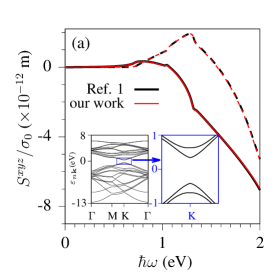
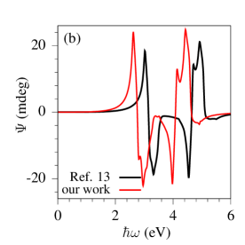
Figure 1: Comparisons between our theory and those in literature. (a) The spectra of $S^{xyz}$ using the method in Ref. 1 (black lines) and in our work (red lines) for a $(2,1,2\,{\rm eV},0,\bm{\delta}_{c})$-TBG. The solid (dashed) curves give the real (imaginary) parts. The insets are the band structure of a gapped TBG. (b) The ellipticity spectra for a $(2,1,0,0,\bm{\delta}_{c})$-TBG using the Hamiltonian provided in Ref. 13 (black lines) and in our work (red lines). The damping energy is adjusted to 25 meV for comparison.

We numerically validate the derived expression by comparing with two theories presented in literature [1, 13]. The first concerns the “sum rules” of $S_{-1}^{dab}=0$ in an undoped topologically trivial insulator at zero temperature, which vanishes automatically for an insulator in the theory by Mahon and Sipe [1]. To get a gapped system, we choose the parameters as $(m,n,\Delta,V_{g},\bm{\delta})=(2,1,2\,{\rm eV},0,\bm{\delta}_{c})$, which generates a bandgap of 0.77 eV. In Fig. 1 (a), we show the spectra of $S^{xyz}$ obtained from our expressions and those from the expression by Mahon and Sipe [1]. The excellent agreement indicates the existence of the sum rule $S_{-1}^{dab}=0$. More specifically, we find $|S_{-1}^{xyz}/\sigma_{0}|\approx 3.17\times 10^{-30}$ ${\rm eV\cdot m}$ with $\sigma_{0}=e^{2}/4\hbar$. Note that such negligible values are obtained with all bands in the model Hamiltonian and with the inclusion of whole BZ. When only half of the bands on both sides of the Fermi level are used in the calculation, for example, we obtain $|S_{-1}^{xyz}/\sigma_{0}|\approx 4.70\times 10^{-17}$ ${\rm eV\cdot m}$. Similarly, it becomes $|S_{-1}^{xyz}/\sigma_{0}|\approx 4.43\times 10^{-17}$ ${\rm eV\cdot m}$, if the calculation is performed for all bands but includes only k points satisfying that the transition energies between the lowest conduction band and the highest valence band are less than 2 eV.

Then we compare the ellipticity spectra obtained from our expressions with those of Morell et al., where a different tight-binding model is used (also listed in Appendix C). As shown in Fig. 1 (b), the results from two tight-binding models are very similar with respect to the spectra shape, except that the locations of the peaks and valleys are shifted, which is ascribed to the different tight-binding parameters.

III.2 Twist angle dependence of $S^{dac}$

Figure 2 (a) and (b) show the spectra of $S^{xyz}$ for the $(m,n,0,0,\bm{\delta}_{c})$-TBG at various $(m,n)$ or twist angles. The spectra for each twist angle consist mainly of two peaks in different regions of photon energies: One is at low photon energies — less than 3 eV — which moves to smaller photon energies for smaller twist angles; the other is at the high-energy region around 4–5 eV, which changes little with twist angles. We find both features are associated with the optical transitions around Van Hove singularity (VHS) points. In TBG, there are two types of VHS: (1) The first is formed by the intersection of the two Dirac cones of the upper and lower graphene layer; it lies in the lowest conduction band and highest valence band, and the transition energy reduces with the decreasing twist angle [18]. (2) The second is inherited from the VHS of each monolayer graphene, for which the energy changes little with twist angle. Because our approach requires the inclusion of all bands and the integration is over the whole BZ, the calculation becomes extremely time consuming for small twisted angles, especially for the “magic angles”, due to the large number of bands.

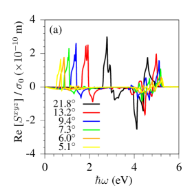
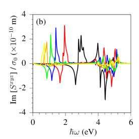
Figure 2: The real (a) and imaginary (b) parts of $S^{xyz}$ for twist angles 21.8^∘, 13.2^∘, 9.4^∘, 7.3^∘, 6.0^∘, and 5.1^∘.

III.3 Chemical potential dependence of $S^{dac}$

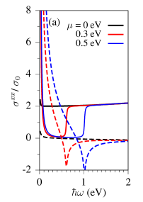
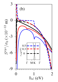
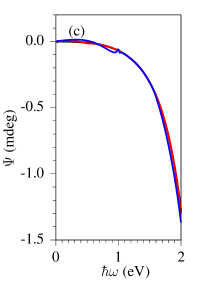
Figure 3: Spectra of (a) $\sigma^{xx}$, (b) $S^{xyz}$, and (c) $\Psi$ for the $(2,1,0,0,\bm{\delta}_{c})$-TBG at different chemical potentials $\mu$ = 0, 0.3 and 0.5 eV. The solid (dashed) curves give the real (imaginary) part. The inset in (b) indicates the position of chemical potentials in the band structure.

Next, we discuss the spectra of $S^{dac}$ for $(2,1,0,0,\bm{\delta}_{c})$-TBG at different chemical potentials $\mu=0$, 0.3, and 0.5 eV. Figure 3 displays the spectra of the linear conductivity $\sigma^{xx}$, the optical activity $S^{xyz}$, and the ellipticity $\Psi$ at the photon energies less than 2 eV, where the chemical potential has significant effects. For undoped TBG, the real part of the linear conductivity has a flat curve with values around $2\sigma_{0}$ [31] and the imaginary part is near zero. Due to the zero gap, the real part of $S^{xyz}$ is nearly proportional to the photon energy, while the imaginary part shows a quadratic relation; these tendencies are very similar to that of a gapped insulator with the gap approaching zero. As the chemical potential increases to 0.3 eV or 0.5 eV, there are free carriers and partially filled bands, which lead to the appearance of the intraband transition for states around the Fermi surface and the Pauli blocked interband transition for states below the Fermi level. For the conductivity $\sigma^{xx}$, the intraband transition gives a Drude contribution $\propto(\omega+i\gamma)^{-1}$ at small photon energies; while for optical activity $S^{xyz}$, the intraband transition lies in the term of $S_{f}$, and it can give a Drude-like contribution $\propto(\omega+i\gamma)^{-2}$; note that, due to free carriers, the term $S_{-1}$ becomes nonzero and contributes by $(\omega+i\gamma)^{-1}$. Therefore, for a finite chemical potential, both $\sigma^{xx}$ and $S^{xyz}$ show behavior that would be divergent for small photon energies. The interband transition leads to an effective band gap $E_{g}\approx 2|\mu|$, which determines the onset of the real part of $\sigma^{xx}$ and the imaginary part of $S^{xyz}$. Similarly, the imaginary part of $\sigma^{xx}$ and the real part of $S^{xyz}$ show divergent peaks in their magnitudes as the photon energy matches the effective gap. Despite of the rich structure in the spectra of $\sigma^{xx}$ and $S^{xyz}$, changing the chemical potential only slightly changes the value of $\Psi$, as shown in Fig. 3 (c).

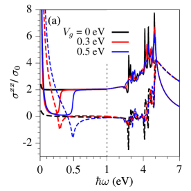
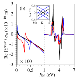
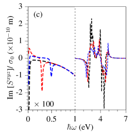
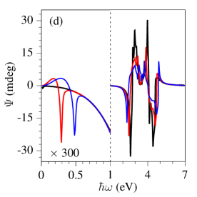
Figure 4: The spectra of (a) $\sigma^{xx}$, (b) real part of $S^{xyz}$, (c) imaginary part of $S^{xyz}$, and (d) $\Psi$ of the $(2,1,0,V_{g},\bm{\delta}_{c})$-TBG for different gate voltages $V_{g}=$ 0, 0.3 and 0.5 eV. Values at $\hbar\omega<1$ eV of $S^{xyz}$ and of $\Psi$ are zoomed in 100 and 300 times, respectively. The inset in (b) illustrates how the gate voltage affects the band structure around the Dirac points.

III.4 Gate voltage dependence of $S^{dac}$

We now turn to the effects of the gate voltage on the optical activity. Figure 4 gives the spectra of linear conductivity $\sigma^{xx}$, optical activity $S^{xyz}$, and the related ellipticity spectra $\Psi$ of $(2,1,0,V_{g},\bm{\delta}_{c})$-TBG for different gate voltages $V_{g}=$ 0, 0.3, 0.5 eV. Note that while the applied gate voltage lowers the symmetry and leads to new nonzero components of the optical activity tensor, we still focus on the component $S^{xyz}$ here. The gate voltage affects the band structure in two ways [29, 30, 32]: one is to split the near degenerate Dirac cones at the Dirac points by lifting the energy of one cone and lowering that of the other, which is analogous to tuning the upper and lower graphene layers with different chemical potentials; and the other is to split both types of VHS points. Therefore, the real part of linear conductivity shows a dip-peak curve at photon energies around $V_{g}$, and its imaginary part shows a valley, due to the inhibited interband transition at the lower-energy region. Here, the effects of the gate voltage on the linear conductivity are similar to those of the chemical potential. As for the the optical activity, a dip-peak structure in the real part and a valley in the imaginary part are observed. However, at the higher energy region, unlike the chemical potential, the gate voltage significantly lowers the peak values of both the linear conductivity and the optical activity. As shown in Fig. 4 (d), the gate voltage has significant effects on the ellipticity spectra, where at the lower energy part a peak appears at energy around $V_{g}$, and at the higher energy part the peak values are reduced with the increasing $V_{g}$.

III.5 Rotation center dependence of $S^{dac}$

Here we consider how the rotation center affects the optical activity tensor. Figure 5 gives the spectra of the three nonzero tensor components for the $(2,1,0,0,\bm{\delta}_{c})$-TBG and $(2,1,0,0,\bm{0})$-TBG. The results show minor differences. This is very similar to the effect of the rotation center on the linear conductivity [26], mostly because the rotation center modifies the band structure very slightly. Although the symmetry analysis gives additional nonzero independent tensor components for $\bm{\delta}=\bm{0}$, their values are about several orders of magnitude smaller than other nonzero components.

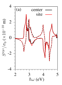
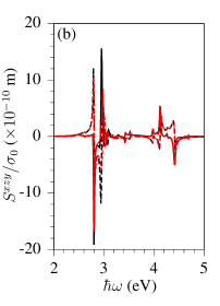
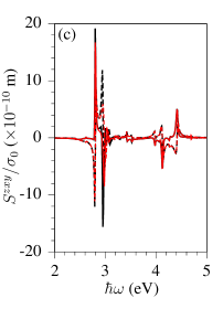
Figure 5: Spectra of optical activity tensors (a) $S^{xyz}$, (b) $S^{xzy}$, and (c) $S^{zxy}$ of TBG with rotation centers at the atom (red curves) and at the center of the hexagon (black curves).

IV Conclusions

We have derived the optical activity tensor by describing the light-matter interaction using the minimal coupling Hamiltonian. Considering the “false divergences” that can arise in this framework, we found that the expression for the prefactor that should vanish is numerically stable and negligibly small if a finite band model Hamiltonian is used and the integration is extended over the whole Brillouin zone. Our expressions are valid for doped systems as well as topological nontrivial materials. We then applied the expressions to a twisted bilayer graphene and studied the effects of the twist angle, chemical potential, gate voltage, and rotation center. The doping can cause a Drude-like contribution to the optical activity tensor for small photon energies, the imaginary parts of the tensor components show onset from the interband transition around the chemical potential induced gap, and the real parts exhibit peaks at the same frequencies. The chemical potential affects the optical activity at very high energies. The gate voltage can modify the band structure at either low or high photon energies, and correspondingly affects the optical activity significantly. We find that the optical activity of twisted bilayer graphene is weakly affected by the rotation center.

Our theory provides a very preliminary study using the minimal coupling Hamiltonian in the single particle approximation. Considering that the excitonic effects are very important for the optical response of two-dimensional materials, it is necessary to extend the theory to include excitonic effects as well as local field corrections [10].

Appendix A Form of Eq. (6)

We briefly explain how to obtain the Hamiltonian in Eq. (6). For an unperturbed Hamiltonian $\hat{H}_{0}(\bm{r},\bm{p})$, which could be used to describe the system with a static magnetic field as well, the interaction between the electrons and the light is introduced by a minimal coupling to a time dependent the vector potential $\bm{A}(\bm{r},t)=\int\frac{d\bm{q}}{(2\pi)^{3}}\bm{A}_{\bm{q}}(t)e^{i\bm{q}\cdot\bm{r}}$ as the Hamiltonian $\hat{H}_{0}(\bm{r},\bm{p}-e\bm{A}(\bm{r},t))$. After expanding it in terms of $\bm{A}_{\bm{q}}(t)$, we formally get

$$\hat{H}_{0}(\bm{r},\bm{p}-e\bm{A}(\bm{r},t))= \hat{H}_{0}(\bm{r},\bm{p})+(-e)\int\frac{d\bm{q}}{(2\pi)^{3}}\hat{\cal V}^{(1);a}_{\bm{q}}(\bm{r},\bm{p})A_{\bm{q}}^{a}(t)$$

$$+\frac{(-e)^{2}}{2}\int\frac{d\bm{q}}{(2\pi)^{3}}\hat{\cal V}^{(2);ab}_{\bm{q}_{1}+\bm{q}_{2}}(\bm{r},\bm{p})A_{\bm{q}_{1}}^{a}(t)A_{\bm{q}_{2}}^{b}(t)+\cdots\,.$$ (18)

For a standard local Hamiltonian $\hat{H}_{0}(\bm{r},\bm{p})=\frac{\bm{p}^{2}}{2m_{0}}+V(\bm{r})$, the expressions of $\hat{\cal V}^{(1)}$ and $\hat{\cal V}^{(2)}$ are

$$\hat{\cal V}^{(1);a}_{\bm{q}}(\bm{r},\bm{p}) =\frac{1}{2}\left(\frac{\hat{\bm{p}}}{m_{0}}e^{i\bm{q}\cdot\bm{r}}+e^{i\bm{q}\cdot\bm{r}}\frac{\hat{\bm{p}}}{m_{0}}\right)\,,$$ (19)

$$\hat{\cal V}^{(2);ab}_{\bm{q}}(\bm{r},\bm{p}) =\delta_{ab}\frac{1}{m_{0}}e^{i\bm{q}\cdot\bm{r}}\,,$$ (20)

respectively. However, in many effective models or ab initio calculations, $\hat{H}_{0}(\bm{r},\bm{p})$ includes the contributions from nonlocal potentials, or perhaps even only its matrix elements between tight-binding basis functions are specified. In such situations, the explicit form of the light-matter interaction term is not very straightforward. To obtain a Hamiltonian that is appropriate for our calculations, and especially to eliminate in practice the “false divergences” that can plague minimal coupling calculations, we find it is necessary to choose the expansion coefficients so that gauge invariance is satisfied, at least up to the linear order of light wave vector $\bm{q}$. For a gauge transformation

$$\boldsymbol{A}(\bm{r},t) \rightarrow\boldsymbol{A}(\bm{r},t)+\nabla g(\bm{r},t)\,,$$ (21a)

$$\phi(\bm{r},t) \rightarrow\phi(\bm{r},t)-\frac{\partial g(\bm{r},t)}{\partial t}\,,$$ (21b)

where $\phi(\bm{r},t)$ is the scalar potential and $g(\bm{r})=g_{\bm{q}}e^{i\bm{q}\cdot\bm{r}}+{\rm c.c.}$ implements the gauge transformation, we require that the form (18) of the coupling be the same whether the new or old potentials are employed. Using

$$\hat{H}_{0}(\bm{r},\bm{p}-e\bm{A}(\bm{r},t)-e\bm{\nabla}g(\bm{r}))=e^{i\frac{e}{\hbar}g(\bm{r})}\hat{H}_{0}(\bm{r},\bm{p}-e\bm{A}(\bm{r},t))e^{-i\frac{e}{\hbar}g(\bm{r})}\,,$$ (22)

and employing a perturbative expansion of the right-hand-side with respect to the orders of $g_{\bm{q}}$, gauge invariance requires that

$$iq^{a}\hat{\cal V}^{(1);a}_{\bm{q}}(\bm{r},\bm{p}) =\frac{1}{i\hbar}[e^{i\bm{q}\cdot\bm{r}},\hat{H}_{0}(\bm{r},\bm{p})]\,,$$ (23)

$$iq_{1}^{a}\hat{\cal V}^{(2);ab}_{\bm{q}_{1}+\bm{q}_{2}}(\bm{r},\bm{p}) =\frac{1}{i\hbar}[e^{i\bm{q}_{1}\cdot\bm{r}},{\cal V}^{(1);b}_{\bm{q}_{2}}(\bm{r},\bm{p})]\,.$$ (24)

It can be verified that the expressions

$$\hat{\cal V}^{(1);a}_{\bm{q}}(\bm{r},\bm{p}) =\frac{1}{2}\left[\hat{v}^{a}(\bm{r},\bm{p})e^{i\bm{q}\cdot\bm{r}}+e^{i\bm{q}\cdot\bm{r}}\hat{v}^{a}(\bm{r},\bm{p})\right]\,,$$ (25)

$$\hat{\cal V}^{(2);ab}_{\bm{q}}(\bm{r},\bm{p}) =\frac{1}{2}\left[\hat{M}^{ab}(\bm{r},\bm{p})e^{i\bm{q}\cdot\bm{r}}+e^{i\bm{q}\cdot\bm{r}}\hat{M}^{ab}(\bm{r},\bm{p})\right]\,,$$ (26)

satisfy the conditions in Eqs. (23, 24) up to the first order in $\bm{q}$. Substituting $\hat{\cal V}^{(1)}$ and $\hat{\cal V}^{(2)}$ in Eqs. (25, 26) back to Eq. (18), we get Eq. (6).

Appendix B Derivation of Eq. (II.2)

For the conductivity in Eq. (13), only the first term at the right hand side include $\bm{q}$. Using the Berry connection

$$\bm{\xi}_{mn\bm{k}} =i\bm{\nabla}_{\bm{q}}U_{m\bm{k},n\bm{k}+\bm{q}}|_{\bm{q}=\bm{0}}\,,$$ (27)

and

$$\left.\frac{\partial}{\partial q^{c}}{\cal V}^{(1);d}_{m\bm{k},n\bm{k}+\bm{q}}\right|_{\bm{q}=0} =\frac{1}{2}\frac{\partial v_{mn\bm{k}}^{a}}{\partial k^{c}}+\frac{i}{2}\sum_{l}\left[v_{ml\bm{k}}^{a}r_{lm\bm{k}}^{c}+r_{nl\bm{k}}^{c}v_{lm\bm{k}}^{a}\right]+\frac{i}{2}\left(\xi_{nn\bm{k}}^{c}+\xi_{mm\bm{k}}^{c}\right)v_{mn\bm{k}}^{a}$$

$$=\frac{1}{2}\frac{\partial v_{mn\bm{k}}^{a}}{\partial k^{c}}+\frac{i}{2}\left\{r_{\bm{k}}^{c},v_{\bm{k}}^{a}\right\}_{mn}+\frac{i}{2}\left(\xi_{nn\bm{k}}^{c}+\xi_{mm\bm{k}}^{c}\right)v_{mn\bm{k}}^{a}\,,$$ (28)

where the off-diagonal terms of $\bm{\xi}_{nm\bm{k}}$ is noted as $\bm{r}_{nm\bm{k}}$, we get

$$\left.\frac{\partial}{\partial q^{c}}\left[{\cal V}^{(1);d}_{m\bm{k},n\bm{k}+\bm{q}}{\cal V}^{(1);a}_{n\bm{k}+\bm{q},m\bm{k}}\right]\right|_{\bm{q}=0}=\frac{1}{2}\frac{\partial(v_{mn\bm{k}}^{d}v_{nm\bm{k}}^{a})}{\partial k^{c}}+\frac{i}{2}v_{mn\bm{k}}^{d}\{r_{\bm{k}}^{c},v_{\bm{k}}^{a}\}_{nm}-\frac{i}{2}\{r_{\bm{k}}^{c},v_{\bm{k}}^{d}\}_{mn}v_{nm\bm{k}}^{a}\,,$$ (29)

with the notation $\{r_{\bm{k}}^{c},v_{\bm{k}}^{a}\}_{nm}=\sum_{l}(r_{nl\bm{k}}^{c}v_{lm\bm{k}}^{a}+v_{nl\bm{k}}^{a}r_{lm\bm{k}}^{c})$.

In calculating $S^{dac}$, the first term in Eq. (29) appears as

$$\propto\int_{\text{BZ}}\frac{d\bm{k}}{(2\pi)^{3}}\frac{\frac{\partial(v_{mn\bm{k}}^{d}v_{nm\bm{k}}^{a})}{\partial k^{c}}f_{mn\bm{k}}}{\hbar\omega^{+}-\hbar\omega_{nm\bm{k}}}=-\int_{\text{BZ}}\frac{d\bm{k}}{(2\pi)^{3}}(v_{mn\bm{k}}^{d}v_{nm\bm{k}}^{a})\frac{\partial}{\partial k^{c}}\frac{f_{mn\bm{k}}}{\hbar\omega^{+}-\hbar\omega_{nm\bm{k}}}\,.$$ (30)

Using all these expressions, we find Eq. (II.2).

Appendix C Expressions of $S_{f}$, $S_{-1}$, $S_{0}$, and $S_{r}$

Substituting Eqs. (15) into Eq. (II.2), we can directly get

$$S^{dac}_{f}(\omega) =g_{s}\frac{|e|^{2}}{2i\omega}\sum_{nm}\int_{\text{BZ}}\frac{d\bm{k}}{(2\pi)^{3}}\frac{v_{mn\bm{k}}^{d}v_{nm\bm{k}}^{a}}{\hbar\omega^{+}-\hbar\omega_{nm\bm{k}}}\frac{\partial(f_{n\bm{k}}+f_{m\bm{k}})}{\partial k^{c}}\,,$$ (31a)

$$S^{dac}_{-1}= -g_{s}\frac{|e|^{2}}{2i\hbar}\sum_{nm}\int_{\text{BZ}}\frac{d\bm{k}}{(2\pi)^{3}}\left[r_{mn\bm{k}}^{d}r_{nm\bm{k}}^{a}(v_{nn\bm{k}}^{c}+v_{mm\bm{k}}^{c})\right.$$

$$\left.-(r_{mn\bm{k}}^{d}\{r_{\bm{k}}^{c},v_{\bm{k}}^{a}\}_{nm}+\{r_{\bm{k}}^{c},v_{\bm{k}}^{d}\}_{mn}r_{nm\bm{k}}^{a})\right]f_{mn\bm{k}}\,,$$ (31b)

$$S_{0}^{dac}= -g_{s}\frac{|e|^{2}}{2i\hbar}\sum_{nm}\int_{\text{BZ}}\frac{d\bm{k}}{(2\pi)^{3}}\left[2r_{mn\bm{k}}^{d}r_{nm\bm{k}}^{a}(v_{nn\bm{k}}^{c}+v_{mm\bm{k}}^{c})\right.$$

$$\left.-(r_{mn\bm{k}}^{d}\{r_{\bm{k}}^{c},v_{\bm{k}}^{a}\}_{nm}+\{r_{\bm{k}}^{c},v_{\bm{k}}^{d}\}_{mn}r_{nm\bm{k}}^{a})\right]\frac{f_{mn\bm{k}}}{\omega_{nm\bm{k}}}\,,$$ (31c)

and

$$S^{dac}_{r}(\omega) =g_{s}\frac{e^{2}\hbar\omega}{2i}\int_{\text{BZ}}\frac{d\bm{k}}{(2\pi)^{3}}\sum_{mn}\frac{X^{dac}_{mn\bm{k}}(\omega)f_{nm\bm{k}}}{\hbar\omega_{mn\bm{k}}(\hbar\omega_{mn\bm{k}}-\hbar\omega^{+})}\,,$$ (31d)

with

$$X^{dac}_{mn\bm{k}}= r_{nm\bm{k}}^{d}\{v^{a}_{\bm{k}},r^{c}_{\bm{k}}\}_{mn}+r_{mn\bm{k}}^{a}\{v^{d}_{\bm{k}},r^{c}_{\bm{k}}\}_{nm}$$

$$-(v_{mm\bm{k}}^{c}+v_{nn\bm{k}}^{c})r_{nm\bm{k}}^{d}r_{mn\bm{k}}^{a}\frac{3\hbar\omega_{mn\bm{k}}-2\hbar\omega}{\hbar\omega_{mn\bm{k}}-\hbar\omega^{+}}\,.$$ (32)

When simplifying the results of Mahon and Sipe [1], we can find all diagonal terms $\bm{\xi}_{nn\bm{k}}$ are canceled out, and only the off-diagonal terms $\bm{r}_{nm\bm{k}}$ remain. The final simplified expression is found to be the same as $S_{r}^{dac}(\omega)$ after combining different terms and alternatively using the relation between $\bm{r}_{nm\bm{k}}$ and $\bm{v}_{nm\bm{k}}$.

For crystals with time-reversal symmetry, the matrix elements satisfy [33]

$$\bm{r}_{nm(-\bm{k})}=\bm{r}_{mn\bm{k}}\,,\quad\bm{v}_{nm(-\bm{k})}=-\bm{v}_{mn\bm{k}}\,.$$ (33)

Using this relation, one can show $S_{0}^{dac}=0$.

Appendix D Tight-binding model for twisted bilayer graphene

The tight-binding Hamiltonian of a commensurate TBG is adopted from the work by Moon and Koshino [26], and slightly modified with the inclusion of the nonequivalent A and B onsite energies. The Hamiltonian used here is different from that used by Morell et al. [13], and the details are listed below briefly.

Starting from a AA stacked bilayer graphene, the TBG is constructed by rotating the upper and lower layers by ${\theta}/{2}$ and $-{\theta}/{2}$, respectively, and then translating the layer 2 relative to the layer 1 by an inplane vector $\bm{\delta}$. Here, $\bm{\delta}=\bm{0}$ and $\bm{\delta}=2(\bm{a}_{1}+\bm{a}_{2})/3$ represent the rotation center at the atom and at the center of hexagon, and correspond to the $D_{3}$ and $D_{6}$ point group, respectively. Taking the lattice vectors of the unrotated graphene as ${\bm{a}}_{1}=a(\sqrt{3}/2,-1/2)$ and ${\bm{a}}_{2}=a(\sqrt{3}/2,1/2)$ with the lattice constant $a\approx 2.46$ Å, the supercell of the commensurate TBG can be described by two integer numbers $(m,n)$ as

$${\bm{A}}_{1}=m{\bm{a}}^{(\nu)}_{1}+n{\bm{a}}^{(\nu)}_{2}\,,$$ (34a)

$${\bm{A}}_{2}=R(\pi/3){\bm{A}}_{1}\,,$$ (34b)

where ${\bm{a}}_{j}^{(\nu)}$ is the rotated lattice vector in the $\nu=\pm$ layer. The corresponding twist angle $\theta$ is calculated through

$$\cos\theta=\frac{m^{2}+n^{2}+4mn}{2(m^{2}+n^{2}+mn)}\,.$$ (35)

Therefore, the tight-binding Hamiltonian is given by

$$\hat{H}_{0}=-\sum_{ij}\left[t(\bm{R}_{i}-\bm{R}_{j})+\delta_{ij}\left(s_{i}\frac{\Delta}{2}+\nu_{i}\frac{V_{g}}{2}\right)\right]\hat{b}_{i}^{\dagger}\hat{b}_{j}\,.$$ (36)

Here ${\bm{R}}_{i}=n_{i}\bm{a}_{1}^{(\nu_{i})}+m_{i}\bm{a}_{2}^{(\nu_{i})}+\bm{\tau}_{\alpha_{i}}^{(\nu_{i})}+\bm{d}^{(\nu_{i})}$ indicates the atom position with an abbreviated index $i=(n_{i}m_{i}\alpha_{i}\nu_{i})$, where $\bm{\tau}_{\alpha_{i}}^{(\nu_{i})}$ is the bias of the $\alpha_{i}=A,B$ atom in the unit cell and $\bm{d}^{(\nu_{i})}$ is the $z$-position of the $\nu_{i}$ layer; $|{\bm{R}}_{i}\rangle$ indicates the $2p_{z}$ orbital at the site $\bm{R}_{i}$; $\Delta$ is the onsite energy with $s_{i}=1$ for $\alpha_{i}=A$ and $-1$ for $\alpha_{i}=B$; and $V_{g}$ gives the layer potential (In experiments, values of $V_{g}$ in TBG were measured to be up to 1 eV, equating to an electric field of roughly 3 V/nm [30, 34]). The hopping term in the work by Moon and Koshino [26] is given by

$$-t(\bm{d})= V_{pp\pi}^{0}\exp\left({-\frac{d-a_{b}}{\delta_{0}}}\right)\cdot\left[1-\left(\frac{\bm{d}\cdot{\bm{e}}_{z}}{d}\right)^{2}\right]$$

$$+V_{pp\sigma}^{0}\exp\left({-\frac{d-d_{0}}{\delta_{0}}}\right)\cdot\left(\frac{\bm{d}\cdot{\bm{e}}_{z}}{d}\right)^{2}\,,$$ (37)

with $V^{0}_{pp\pi}\approx-2.7$ eV, $V^{0}_{pp\sigma}\approx 0.48$ eV, $a_{0}=a/\sqrt{3}\approx 1.42$ Å, $d\approx 3.35$ Å, and $\delta_{0}=0.184~{}a\approx 0.45$ Å. In contrast, the hopping term in the work by Morell et al. [13] is written as

$$-t(\bm{d})=\gamma\sum_{i,j}\exp\left[{-\beta(|{\bm{d}}|-d)}\right]\,,$$ (38)

with $\gamma=-0.39$ eV and $\beta=3$. The position operator $\hat{\bm{r}}$ is

$$\hat{\bm{r}}=\sum_{i}\bm{R}_{i}\hat{b}_{i}^{\dagger}\hat{b}_{i}\,.$$ (39)

The velocity operator $\hat{\bm{v}}$ is then

$$\hat{\bm{v}} =\frac{1}{i\hbar}[\hat{\bm{r}},\hat{H}_{0}]\,.$$ (40)

Each supercell of TBG contains $N=4(n^{2}+m^{2}+nm)$ carbon atoms, which can be identified by biases $\bm{t}_{l}$ with an index $l=1,2,\cdots,N$. By matching $\bm{R}_{i}=p_{i}\bm{A}_{1}+q_{i}\bm{A}_{2}+\bm{t}_{l_{i}}$, the bias $\bm{t}_{l_{i}}$ can be obtained and the abbreviated index $i$ also stands for integers $(p_{i}q_{i}l_{i})$. After performing the transformation

$$\hat{b}_{pql} =\sqrt{\frac{\Omega}{(2\pi)^{2}}}\int d\bm{k}e^{i\bm{k}\cdot(p\bm{A}_{1}+q\bm{A}_{2})}\hat{c}_{l\bm{k}}\,,$$ (41)

the Hamiltonian becomes

$$\hat{H}_{0}=\sum_{l_{1}l_{2}}\int d\bm{k}H_{l_{1}l_{2}\bm{k}}^{0}\hat{c}_{l_{1}\bm{k}}^{\dagger}\hat{c}_{l_{2}\bm{k}}\,,$$ (42)

with

$$H_{l_{1}l_{2}\bm{k}}^{0}=\sum_{pq}e^{-i\bm{k}\cdot(p\bm{A}_{1}+q\bm{A}_{2})}t(\bm{R}_{pql_{1}}-\bm{R}_{00l_{2}})+\delta_{l_{1},l_{2}}\left[s^{(00l_{1})}\frac{\Delta}{2}+\nu^{(00l_{1})}\frac{V_{g}}{2}\right]\,.$$ (43)

It can be diagonalized into

$$\hat{H}_{0}=\sum_{s}\int d\bm{k}\varepsilon_{s\bm{k}}\hat{a}_{s\bm{k}}^{\dagger}\hat{a}_{s\bm{k}}\,,$$ (44)

through the transformation

$$\hat{c}_{l\bm{k}} =\sum_{s}C_{s\bm{k};l}\hat{a}_{s\bm{k}}\,,$$ (45)

where the wavefunctions $C_{s\bm{k};l}$ satisfy the eigenequations

$$\sum_{l_{2}}H_{l_{1}l_{2}\bm{k}}C_{s\bm{k};l_{2}}=\varepsilon_{s\bm{k}}C_{s\bm{k};l_{1}}\,,$$ (46)

with the band index $s$ and eigenenergy $\varepsilon_{s\bm{k}}$. Similar transformation gives the velocity operator as

$$\hat{\bm{v}} =\int d\bm{k}\sum_{s_{1}s_{2}}\bm{v}_{s_{1}s_{2}\bm{k}}\hat{a}_{s_{1}\bm{k}}^{\dagger}\hat{a}_{s_{2}\bm{k}}\,.$$ (47)

References

• Mahon and Sipe [2020] P. T. Mahon and J. E. Sipe, From magnetoelectric response to optical activity, Phys. Rev. Research 2, 043110 (2020).
• Rérat and Kirtman [2021] M. Rérat and B. Kirtman, First-principles calculation of the optical rotatory power of periodic systems: Application on $\alpha$-quartz, tartaric acid crystal, and chiral (n,m)-carbon nanotubes, J. Chem. Theory Comput. 17, 4063 (2021).
• Ohnoutek et al. [2021] L. Ohnoutek, H.-H. Jeong, R. R. Jones, J. Sachs, B. J. Olohan, D.-M. Răsădean, G. D. Pantoş, D. L. Andrews, P. Fischer, and V. K. Valev, Optical activity in third-harmonic Rayleigh scattering: A new route for measuring chirality, Laser Photonics Rev. 15, 2100235 (2021).
• Beaulieu et al. [2018] S. Beaulieu, A. Comby, D. Descamps, B. Fabre, G. A. Garcia, R. Géneaux, A. G. Harvey, F. Légaré, Z. Mašín, L. Nahon, A. F. Ordonez, S. Petit, B. Pons, Y. Mairesse, O. Smirnova, and V. Blanchet, Photoexcitation circular dichroism in chiral molecules, Nat. Phys. 14, 484 (2018).
• Ahn et al. [2020] J. Ahn, S. Ma, J.-Y. Kim, J. Kyhm, W. Yang, J. A. Lim, N. A. Kotov, and J. Moon, Chiral 2D organic inorganic hybrid perovskite with circular dichroism tunable over wide wavelength range, J. Am. Chem. Soc. 142, 4206 (2020).
• Tsirkin et al. [2018] S. S. Tsirkin, P. A. Puente, and I. Souza, Gyrotropic effects in trigonal tellurium studied from first principles, Phys. Rev. B 97, 035158 (2018).
• Guo et al. [2022] Z. Guo, J. Li, J. Liang, C. Wang, X. Zhu, and T. He, Regulating optical activity and anisotropic second-harmonic generation in zero-dimensional hybrid copper halides, Nano Lett. 22, 846 (2022).
• Zhong et al. [1993] H. Zhong, Z. H. Levine, D. C. Allan, and J. W. Wilkins, Band-theoretic calculations of the optical-activity tensor of $\alpha$-quartz and trigonal Se, Phys. Rev. B 48, 1384 (1993).
• Malashevich and Souza [2010] A. Malashevich and I. Souza, Band theory of spatial dispersion in magnetoelectrics, Phys. Rev. B 82, 245118 (2010).
• Jönsson et al. [1996] L. Jönsson, Z. H. Levine, and J. W. Wilkins, Large local-field corrections in optical rotatory power of quartz and Selenium, Phys. Rev. Lett. 76, 1372 (1996).
• Sipe and Ghahramani [1993] J. E. Sipe and E. Ghahramani, Nonlinear optical response of semiconductors in the independent-particle approximation, Phys. Rev. B 48, 11705 (1993).
• Mahon et al. [2019] P. T. Mahon, R. A. Muniz, and J. E. Sipe, Microscopic polarization and magnetization fields in extended systems, Phys. Rev. B 99, 235140 (2019).
• Morell et al. [2017] E. S. Morell, L. Chico, and L. Brey, Twisting Dirac fermions: Circular dichroism in bilayer graphene, 2D Mater. 4, 035015 (2017).
• Trambly de Laissardière et al. [2012] G. Trambly de Laissardière, D. Mayou, and L. Magaud, Numerical studies of confined states in rotated bilayers of graphene, Phys. Rev. B 86, 125413 (2012).
• Morell et al. [2010] E. S. Morell, J. D. Correa, P. Vargas, M. Pacheco, and Z. Barticevic, Flat bands in slightly twisted bilayer graphene: Tight-binding calculations, Phys. Rev. B 82, 121407 (2010).
• Trambly de Laissardière et al. [2010] G. Trambly de Laissardière, D. Mayou, and L. Magaud, Localization of Dirac electrons in rotated graphene bilayers, Nano Lett. 10, 804 (2010).
• Andrei and MacDonald [2020] E. Y. Andrei and A. H. MacDonald, Graphene bilayers with a twist, Nat. Mater. 19, 1265 (2020).
• Zheng et al. [2022] Z. Zheng, Y. Song, Y. W. Shan, W. Xin, and J. L. Cheng, Optical coherent injection of carrier and current in twisted bilayer graphene, Phys. Rev. B 105, 085407 (2022).
• Tepliakov et al. [2020] N. V. Tepliakov, A. V. Orlov, E. V. Kundelev, and I. D. Rukhlenko, Twisted bilayer graphene quantum dots for chiral nanophotonics, J. Phys. Chem. C 124, 22704 (2020).
• Kim et al. [2016] C.-J. Kim, A. Sánchez-Castillo, Z. Ziegler, Y. Ogawa, C. Noguez, and J. Park, Chiral atomically thin films, Nat. Nanotechnol. 11, 520 (2016).
• Cheng et al. [2017] J. L. Cheng, N. Vermeulen, and J. E. Sipe, Second order optical nonlinearity of graphene due to electric quadrupole and magnetic dipole effects, Sci. Rep. 7, 43843 (2017).
• Li et al. [2013] Z. Li, M. Mutlu, and E. Ozbay, Chiral metamaterials: from optical activity and negative refractive index to asymmetric transmission, J. Opt. 15, 023001 (2013).
• Boyd [2008] R. W. Boyd, Nonlinear Optics, 3rd ed. (Academic, 2008).
• Mahan [2000] G. D. Mahan, Nonzero Temperatures. In: Many-Particle Physics. (Physics of Solids and Liquids. Springer, Boston, MA., 2000).
• Pizzi et al. [2020] G. Pizzi, V. Vitale, R. Arita, S. Blügel, F. Freimuth, G. Géranton, M. Gibertini, D. Gresch, C. Johnson, T. Koretsune, J. Ibañez-Azpiroz, H. Lee, J.-M. Lihm, D. Marchand, A. Marrazzo, Y. Mokrousov, J. I. Mustafa, Y. Nohara, Y. Nomura, L. Paulatto, S. Poncé, T. Ponweiser, J. Qiao, F. Thöle, S. S. Tsirkin, M. Wierzbowska, N. Marzari, D. Vanderbilt, I. Souza, A. A. Mostofi, and J. R. Yates, Wannier90 as a community code: new features and applications, Journal of Physics: Condensed Matter 32, 165902 (2020).
• Moon and Koshino [2013] P. Moon and M. Koshino, Optical absorption in twisted bilayer graphene, Phys. Rev. B 87, 205404 (2013).
• McCann [2006] E. McCann, Asymmetry gap in the electronic band structure of bilayer graphene, Phys. Rev. B 74, 161403 (2006).
• Cappelluti et al. [2012] E. Cappelluti, L. Benfatto, M. Manzardo, and A. B. Kuzmenko, Charged-phonon theory and Fano effect in the optical spectroscopy of bilayer graphene, Phys. Rev. B 86, 115439 (2012).
• Nicol and Carbotte [2008] E. J. Nicol and J. P. Carbotte, Optical conductivity of bilayer graphene with and without an asymmetry gap, Phys. Rev. B 77, 155409 (2008).
• Brun and Pedersen [2015] S. J. Brun and T. G. Pedersen, Intense and tunable second-harmonic generation in biased bilayer graphene, Phys. Rev. B 91, 205405 (2015).
• Tabert and Nicol [2013] C. J. Tabert and E. J. Nicol, Optical conductivity of twisted bilayer graphene, Phys. Rev. B 87 (2013).
• Yu et al. [2019] K. Yu, N. Van Luan, T. Kim, J. Jeon, J. Kim, P. Moon, Y. H. Lee, and E. J. Choi, Gate tunable optical absorption and band structure of twisted bilayer graphene, Phys. Rev. B 99, 241405 (2019).
• Sipe and Shkrebtii [2000] J. E. Sipe and A. I. Shkrebtii, Second-order optical response in semiconductors, Phys. Rev. B 61, 5337 (2000).
• Zhang et al. [2009] Y. Zhang, T.-T. Tang, C. Girit, Z. Hao, M. C. Martin, A. Zettl, M. F. Crommie, Y. R. Shen, and F. Wang, Direct observation of a widely tunable bandgap in bilayer graphene, Nature 459, 820 (2009).