Robust Graph Structure Learning via
Multiple Statistical Tests

Abstract

Graph structure learning aims to learn connectivity in a graph from data. It is particularly important for many computer vision related tasks since no explicit graph structure is available for images for most cases. A natural way to construct a graph among images is to treat each image as a node and assign pairwise image similarities as weights to corresponding edges. It is well known that pairwise similarities between images are sensitive to the noise in feature representations, leading to unreliable graph structures. We address this problem from the viewpoint of statistical tests. By viewing the feature vector of each node as an independent sample, the decision of whether creating an edge between two nodes based on their similarity in feature representation can be thought as a single statistical test. To improve the robustness in the decision of creating an edge, multiple samples are drawn and integrated by multiple statistical tests to generate a more reliable similarity measure, consequentially more reliable graph structure. The corresponding elegant matrix form named $\mathcal{B}$-Attention is designed for efficiency. The effectiveness of multiple tests for graph structure learning is verified both theoretically and empirically on multiple clustering and ReID benchmark datasets. Source codes are available at https://github.com/Thomas-wyh/B-Attention.

1 Introduction

Graph structure learning plays an important role in Graph Convolutional Networks (GCNs). It seeks to discover underlying graph structures for better graph representation learning when graph structures are unavailable, noisy or corrupted. These issues are typical in the field of vision tasks wang2019linkage ; yang2019learning ; yang2020learning ; guo2020density ; nguyen2021clusformer ; shen2021starfc ; wang2022adanets ; chum2007total ; luo2019spectral ; zhong2017re ; sarfraz2018pose . As an example, there is no explicit graph structure between photos in your phone albums, so the graph-based approaches guo2020density ; nguyen2021clusformer ; wang2022adanets in photo management softwares seek to learn graph structure. A popular research direction on it is to consider graph structure learning as similarity measure learning upon the node embedding space GNNBook2022 . They learn weighted adjacency matrices guo2020density ; nguyen2021clusformer ; chen2019graphflow ; chen2020reinforcement ; on2020cut ; yang2018glomo ; huang2020location ; chen2020iterative ; henaff2015deep ; li2018adaptive as graphs and feed them to GCNs to learn representations.

However, the main problem of the above weighted-based methods is that weights are not always accurate and reliable: two nodes with smaller associations may have a higher weight score than those with larger associations. The root of this problem is closely related to the noise in the high dimensional feature vectors extracted by the deep learning model, as similarities between nodes are usually decided based on their feature vectors. The direct consequence of using an inaccurate graph structure is so called feature pollution wang2022adanets , leading to a performance degradation in downstream tasks. In our empirical studies, we found that close to $1/3$ of total weights are assigned to noisy edges when unnormalized cosine similarities between feature vectors are used to calculate weights.

Many methods have been developed to improve similarity measure between nodes in graph, including adding learnable parameters chen2019graphflow ; huang2020location ; chen2020iterative , introducing nonlinearity chen2020reinforcement ; on2020cut ; yang2018glomo , Gaussian kernel functions henaff2015deep ; li2018adaptive and self-attention vaswani2017attention ; Choi2020LearningTG ; guo2020density ; nguyen2021clusformer . Despite the progress, they are limited to modifying similarity function, without explicitly addressing the noise in feature vectors, a more fundamental issue for graph structure learning. One way to capture the noise in feature vectors is to view the feature vector of each node as an independent sample from some unknown distribution associated with each node. As a result, the similarity score between two nodes can be thought as the expectation of a test to decide if two nodes share the same distribution. Since, only one vector is sampled for each node in the above methods, the statistical test is essentially based on a single sample from both nodes, making the calculated weights inaccurate and unreliable.

An possible solution towards addressing the noise in feature vectors is to run multiple tests, a common approach to reduce variance in sampling and decision making bienayme1853considerations ; chernoff1952measure ; hoeffding1956distribution . Multiple samples are drawn for each node, and each sample can be used to run an independent test to decide if two nodes share the same distribution. Based on the results from multiple tests, we develop a novel and robust similarity measure that significantly improves the robustness and reliability of calculated weights. This paper will show how to accomplish multiple tests in the absence of graph structures and theoretically prove why the proposed approach can produce a better similarity measure under specified conditions. This similarity measure is also crafted into an efficient and elegant form of matrix, named $\mathcal{B}$-Attention. $\mathcal{B}$-Attention utilizes the fourth order statistics of the features, which is a significant difference with popular attentions. Benefiting from a better similarity measure produced by multiple tests, graph structures can be significantly improved, resulting in better graph representations and therefore boosting the performance of downstream tasks. We empirically verify the effectivness of the proposed method over the task of clustering and ReID.

In summary, this paper makes the following three major contributions: (1) To the best of our knowledge, this is the first paper to address inaccurate edge weights problem by statistical tests on the task of graph structure learning over images. (2) A novel and robust similarity measure is proposed based on multiple tests, proven theoretically to be superior and designed in an elegant matrix form to improve graph structure quality. (3) Extensive experiments further verify the robustness of the graph structure learning method against noise. State-of-the-art (SOTA) performances are achieved on multiple clustering and ReID benchmarks with the learned graph structures.

2 Methodology

To handle the noise in feature vectors, we model the feature vector of each node as a sample drawn from the underlying distribution associated with that node, and the similarity score between two nodes as the expectation of a statistical test. The test is to compare their similarity to a given threshold to decide if two nodes share the same distribution and that decision can be captured by a binary Bernoulli random variable. The comparison in statistical test may lead to error edges, i.e., noisy edges (an edge connects two nodes of different categories) or missing edges (two nodes of the same category should be connected but are not). The superiority of the similarity measure can be revealed by comparing the probability of creating an error edge. The proposed similarity measure will be introduced in Section 2.2, and its further design in matrix form will be presented in Section 2.3.

2.1 Preliminary

Chernoff Bounds.

Sums of random variables have been studied for a long time bienayme1853considerations ; chernoff1952measure ; hoeffding1956distribution . Chernoff Bounds chernoff1952measure provide sharply decreasing bounds that are in the exponential form on tail distributions of sums of independent random variables. It is a widely used fundamental tool in mathematics and computer science kearns1994introduction ; motwani1995randomized . An often used and looser form of Chernoff Bounds is as follows.

Lemma 1 (Chernoff Bounds chernoff1952measure ).

Suppose $X_{i}$ is a binary random variable taking value in set $\{0,1\}$ with $\mathbb{P}(X_{i}=1)=p_{i}$ . Define $X=\sum_{1}^{n}X_{i}$ where $\{X_{1},X_{2},\cdots,X_{n}\}$ are independently sampled. Then for any $0<\epsilon<1$,

$$\mathbb{P}(X\geq(1+\epsilon)\mu) \leq e^{-\frac{\epsilon^{2}}{3}\mu},$$

$$\mathbb{P}(X\leq(1-\epsilon)\mu) \leq e^{-\frac{\epsilon^{2}}{3}\mu}\ .$$

It shows that with a high probability $1-\delta$, we have $X\leq(1+\epsilon)\mu$, or $X\geq(1-\epsilon)\mu$, where $\delta=e^{-\frac{\epsilon^{2}}{3}}$.

GCNs.

A GCN network normally consists of multiple GCN layers. Given an input graph $\mathcal{G}\left(\mathbf{X},\mathbf{A}\right)$ with $L$ vertices, the output of a normal GCN layer kipf2017semi is:

$$\mathbf{X}^{{}^{\prime}} =\sigma(\mathbf{\tilde{D}}^{-\frac{1}{2}}\mathbf{\tilde{A}}\mathbf{\tilde{D}}^{-\frac{1}{2}}\mathbf{X}\mathbf{W}_{l}),\quad\textrm{where}\ \mathbf{\tilde{A}} =\mathbf{A}+\mathbf{I},\ \mathbf{\tilde{D}}_{ii}=\sum_{j=1}^{L}\mathbf{\tilde{A}}_{i,j},$$ (1)

$\mathbf{X}\in\mathbb{R}^{L\times M}$ is input vertex features with $M$ dimensions, $\mathbf{A}\in\mathbb{R}^{L\times L}$ is their adjacency matrix; $\mathbf{I}\in\mathbb{R}^{L\times L}$ is an identity matrix, $\mathbf{\tilde{D}}\in\mathbb{R}^{L\times L}$ is the diagonal degree matrix of $\mathbf{\tilde{A}}$; $\mathbf{W}_{l}\in\mathbb{R}^{M\times M^{\prime}}$ is a trainable matrix, and $\sigma(\cdot)$ is an activation function such as ReLU glorot2011deep ; $\mathbf{X}^{{}^{\prime}}\in\mathbb{R}^{L\times M^{\prime}}$ is the output vertex features with $M^{\prime}$ dimensions, $M^{\prime}=M$ in this work.

2.2 Multiple tests on similarity measure

Let $\mathcal{V}=\left\{v_{1},v_{2},...,v_{N}\right\}$ be the collection of $N$ nodes. Each node is assumed to be in one of two categories: $+1$ or $-1$ for simplicity. For each node $v_{i}$, the subset of candidate nodes to connect it is denoted by $\mathcal{V}_{i}$. This subset can be decided by a simple criterion such as by $k$ nearest neighbours. When calculating the proposed similarity between $v_{i}$ and $v_{j}\in\mathcal{V}_{i}$, the common candidate nodes between $v_{i}$ and $v_{j}$, i.e., $\mathcal{V}_{i,j}=\mathcal{V}_{i}\cap\mathcal{V}_{j}$ are first identified. The nodes in the $\mathcal{V}_{i,j}$ are treated as the multiple samples drawn for the comparison of $v_{i}$ and $v_{j}$. Then, each $v_{k}\in\mathcal{V}_{i,j}$ performs single test twice, one for $v_{k}$ and $v_{i}$ and one for $v_{k}$ and $v_{j}$. The single test here is a comparison using the pairwise similarity based on the features of $v_{k}$ and $v_{i}$, or $v_{k}$ and $v_{j}$. The pairwise similarity can be cosine similarity, Gaussian kernel similarity or any other form, and is denoted by Sim-S. The proposed similarity score between $v_{i}$ and $v_{j}$ increases by one if the two tests yield $C(v_{i})=C(v_{k})$ and $C(v_{k})=C(v_{j})$, and zero otherwise, where $C(v)$ is the category of node $v$. It contains multiple single tests, hence the name multiple tests, corresponding similarity measure denoted by Sim-M.

For the convenience of analysis, a few assumptions are further introduced. First, the size of $\mathcal{V}_{i,j}$ is $m$, and among the nodes in $\mathcal{V}_{i,j}$ , $\alpha m$ nodes share the same category as $v_{i}$ and $\left(1-\alpha\right)m$ nodes belong to the opposite category, with $\alpha>\frac{1}{2}$. For any node $v_{j}\in\mathcal{V}_{i}$, its probability of being connected with $v_{i}$, according to the statistical test, is $q\in\left[0,1\right]$ if $C(v_{i})\neq C(v_{j})$, and the probability increases to $1\geq p>q$ if $C(v_{i})=C(v_{j})$. This section will show that, if $m$ is sufficiently large (i.e., enough number of tests can be run), there will exist an appropriate threshold for the Sim-M such that the number of error edges can be reduced significantly compared to Sim-S.

Proposition 1.

For the single test method, in expectation, the number of noisy edges $\mathbb{E}\{N_{\mathrm{noisy}}\}=\left(1-\alpha\right)qm$ and the number of missing edges $\mathbb{E}\{N_{\mathrm{miss}}\}=\alpha\left(1-p\right)m$.

The theorem below shows that both $\mathbb{E}\{N_{\mathrm{noisy}}\}$ and $\mathbb{E}\{N_{\mathrm{miss}}\}$ can be reduced by a significant portion when $m$ is large enough.

Theorem 1.

Suppose $\gamma>1$ and

$$m>\frac{3((p+q)^{2}+(2\alpha-1)(p^{2}-q^{2}))^{2}}{pq((p-q)^{2}+(2\alpha-1)(p^{2}-q^{2}))^{2}}\log(\frac{\gamma}{\min((1-\alpha)q,\alpha(1-p))}),$$ (2)

We have $\mathbb{E}\{N_{\mathrm{noisy}}\}=\left(1-\alpha\right)qm/\gamma$ and $\mathbb{E}\{N_{\mathrm{miss}}\}=\alpha\left(1-p\right)m/\gamma$ .

Proof.

Consider node $v_{i}$ and one of its candidate node $v_{j}\in\mathcal{V}_{i}$. $S_{i,j}^{k}$ is denoted as the similarity score between $v_{i}$ and $v_{j}$ based on the statistical test with respect to $v_{k}$. As shown in Figure 2, $v_{k}$ may be of the same category as $v_{i}$ or not (denoted by ${v^{\prime}}_{k}$ for a better show). Evidently, $\mathbb{E}[S_{i,j}^{k}]=pq$ if $C(v_{i})\neq C(v_{j})$, and $\mathbb{E}[S_{i,j}^{k}]=\alpha p^{2}+(1-\alpha)q^{2}$ if $C(v_{i})=C(v_{j})$ .

The Sim-M between $v_{i}$ and $v_{j}$ is defined as:

$$S_{i,j}=\frac{1}{m}\sum_{k\in\mathcal{V}_{i,j}}S_{i,j}^{k}.$$ (3)

Using the Chernoff Bounds chernoff1952measure , we have with a probability $1-\delta$,

$$\left\{\begin{array}[]{ll}S_{i,j}=\frac{1}{m}\sum_{k\in V_{i,j}}S_{k}\leq(1+\sqrt{\frac{3log(1/\delta)}{pqm}})pq,&C(v_{i})\neq C(v_{j}),\\ S_{i,j}=\frac{1}{m}\sum_{k\in V_{i,j}}S_{k}\geq(1-\sqrt{\frac{3log(1/\delta)}{(\alpha p^{2}+(1-\alpha)q^{2})m}})(\alpha p^{2}+(1-\alpha)q^{2}),&C(v_{i})=C(v_{j}),\end{array}\right.$$ (4)

By assuming that $m$ is large enough, i.e.,

$$\sqrt{\frac{3\log{(1/\delta)}}{pqm}}<\frac{(p-q)^{2}+(2\alpha-1)(p^{2}-q^{2})}{(p+q)^{2}+(2\alpha-1)(p^{2}-q^{2})},$$ (5)

by choosing the similarity threshold

$$S_{t}=(1+\sqrt{\frac{3log(1/\delta)}{pqm}})\frac{pq}{2}+(1-\sqrt{\frac{3log(1/\delta)}{(\alpha p^{2}+(1-\alpha)q^{2})m}})\frac{\alpha p^{2}+(1-\alpha)q^{2}}{2},$$ (6)

only with a probability $\delta$, we will miss a correct edge, and with a probability $\delta$ we will introduce a noisy edge. We complete the proof by substituting $\delta$ in Equation 5 with

$$\delta\triangleq\frac{1}{\gamma}\min((1-\alpha)q,\alpha(1-p)).$$ (7)

We can guarantee that the Sim-M between two nodes from the same category is strictly larger than that for two nodes from different categories, leading to the distillation of all noisy edges. ∎

2.3 Multiple tests on GCNs

Figure 1: Illustration of $\mathbb{E}[S_{i,j}^{k}]$ in Sim-M on two nodes from different categories and the same category. Nodes of different colors are from different categories.

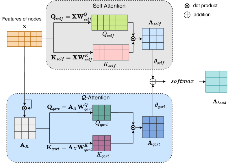
Figure 2: Illustration of the $\mathcal{B}$-Attention mechanism. The self-attention part is the same as that in Transformers. The $\mathcal{Q}$-Attention part generates $\mathbf{A}_{X}$ and then pay attention to it to generate the $\mathbf{A}_{qart}$. The two output attention maps are fused as the final output $\mathbf{A}_{band}$.

With a better similarity measure prototype above, we further craft it into an elegant and efficient matrix form for adaptation of graph structure learning in the real-world. The analysis in Theorem 1 can be easily extended to real similarities, instead of binary simiarities, by using the generalized version of Chernoff inequality detailed in Section E of Appendix. Given the L2 normalized original node features $\mathbf{X}$, the idea of Sim-S can be implemented by inner product of features, i.e. $\mathbf{A}_{X}=\mathbf{X}\mathbf{X}^{T}$. The twice-run tests on each node can be achieved by $\mathbf{A}_{X}$ multiplying itself. Inspired by the design of popular Transformers vaswani2017attention , some learnable parameters are also introduced. It contains the fourth-order statistics of features, which is a significant difference, since self-attention only has second-order. If self-attention is regarded as Duet of Attention, our method is analogous to Quertet of Attention ($\mathcal{Q}$-Attention for short). The vectorized representation of Equation 3, $\mathcal{Q}$-Attention $\mathbf{A}_{qart}\in\mathbb{R}^{L\times L}$, is then implemented as follows:

$$\mathbf{A}_{qart}=\mathbf{Q}_{qart}\mathbf{K}^{T}_{qart},\quad\textrm{where}\ \mathbf{Q}_{qart}=\mathbf{A}_{X}\mathbf{W}^{Q}_{qart},\ \mathbf{K}_{qart}=\mathbf{A}_{X}\mathbf{W}^{K}_{qart},$$ (8)

$\mathbf{W}^{Q}_{qart}\in\mathbb{R}^{L\times L^{\prime}}$ and $\mathbf{W}^{K}_{qart}\in\mathbb{R}^{L\times L^{\prime}}$ are learnable weights, $L^{\prime}=L$ in this work. L2 normalization is also applied to $\mathbf{A}_{X}$.

Motivated by the further enhancements from combinations of intrinsic graph structures and implicit graph structures in literature li2018adaptive ; chen2020iterative ; liu2020retrieval , the self-attention can play an intrinsic role to fuse with the $\mathcal{Q}$-Attention in vision tasks, although no intrinsic graph structure exists between images at all. The self-attention part is the same as that in Transformers vaswani2017attention . The attention map $\mathbf{A}_{self}\in\mathbb{R}^{L\times L}$ is:

$$\mathbf{A}_{self}=\frac{\mathbf{Q}_{self}{\mathbf{K}_{self}}^{T}}{\sqrt{M^{d}}},\quad\textrm{where}\ \mathbf{Q}_{self}=\mathbf{X}\mathbf{W}^{Q}_{self},\ \mathbf{K}_{self}=\mathbf{X}\mathbf{W}^{K}_{self},$$ (9)

$\mathbf{W}^{Q}_{self}\in\mathbb{R}^{M\times M^{d}}$ and $\mathbf{W}^{K}_{self}\in\mathbb{R}^{M\times M^{d}}$ are the learnable weights, $M^{d}$ is the dimension of query and key features. The combined form blends the duet and quartet of attention, hence the name Band of Attention ($\mathcal{B}$-Attention for short). The overview of $\mathcal{B}$-Attention mechanism is shown in Figure 2.

The fusion of $\mathbf{A}_{self}$ and $\mathbf{A}_{qart}$ is defined as (where $\textrm{softmax}(\cdot)$ is a softmax function):

$$\mathbf{A}_{band}=\textrm{softmax}(\theta_{qart}\mathbf{A}_{qart}+\theta_{self}\mathbf{A}_{self}).$$ (10)

When combined with the neural network layer in Equation 1, the final form is:

$$\mathbf{X^{\prime}}=\sigma(\mathbf{A}_{band}\mathbf{X}\mathbf{W}_{l}).$$ (11)

In real implementation, considering the graph size can be very large for large-scale datasets, sub-graph sampling strategy wang2022adanets ; wang2019dgl is adopted to make it more computationally efficient and scalable. In particular, $k_{seed}$ nodes are first selected as seeds from a dataset in each sampling step. Then the seed nodes together with their $k$ nearest neighbours ($k$NN) cover1967nearest form the nodes of a sub-graph. As a result, Equations 8 and 9 are applied to the sub-graph during training and inference. For a dataset of size $N_{d}$, it takes about $N_{d}/k_{seed}$ iterations to process the whole dataset on average. The pseudo code for self-attention and $\mathcal{Q}$-Attention is detailed in Section D of Appendix.

3 Experiments

Experiments are designed with three levels. Firstly, experiments are conducted to analyse the advantage of Sim-M over that of Sim-S and its robustness to noise. Secondly, armed with multiple tests on GCNs, i.e., $\mathcal{B}$-Attention is further investigated in comparison with the self-attention and a commonly used form of GCNs on robustness and superiority. Ablation experiments are then conducted to study how each part of $\mathcal{B}$-Attention contributes to and influences the performance. Finally, with the robust graph structure learned by $\mathcal{B}$-Attention, comparison experiments in downstream graph-based clustering and ReID tasks are conducted to evaluate the benefits of the proposed approach.

3.1 Experimental setups

Datasets

Experiments are conducted on commonly used visual datasets with three different types of objects, i.e., MS-Celeb guo2016ms  (human faces), MSMT17 wei2018person  (human bodies) and VeRi-776 7553002  (vehicles), to verify the generalization of the proposed method. In these datasets, each sample has a specific category, and most categories have rich samples. The tasks on these datasets are popular and representative in computer vision. It is worth noting that MS-Celeb is divided into 10 parts by identities (Part0-9): Part0 for training and Part1-9 for testing, to maintain comparability and consistency with previous works yang2019learning ; yang2019learning ; guo2020density ; wang2022adanets ; nguyen2021clusformer ; shen2021starfc . Details of the dataset are in Section A.1.

Metrics

The Area Under the Curve (AUC) is adopted to directly evaluate the discriminatory power of similarity measures between node pairs. Edge Noise Rate (ENR) illustrates the amount of noise in graphs quantitatively. For node $v_{i}$, $\mathbf{ENR}=\frac{N^{noise}_{i}}{N^{all}_{i}}$, where $N^{noise}_{i}$ is the number of noisy edges and $N^{all}_{i}$ is the amount of all edges for $v_{i}$. The average ENR is defined as the average of the ENRs of all nodes. The feature quality of GCNs output is investigated to prove the effectiveness of graph structure learning: The mean Average Precision (mAP) zhu2004recall is used from the perspective of identification and ROC curves are shown from the perspective of verification. The higher the quality of the features the better the graph structure learning. In downstream ReID tasks, mAP^R and Rank1 accuracy (R1) are used. Compared to mAP, mAP^R additionally takes into account the camera id information, i.e., samples from the same camera as the probe will not be counted in evaluation. BCubed ($\mathbf{F_{B}}$) bagga1998algorithms ; amigo2009comparison and Pairwise ($\mathbf{F_{P}}$) shi2018face F-scores are used for evaluating clustering tasks.

3.2 Effectiveness of the Sim-M

Table 1: Average ENRs of different $k$ values and the AUC of Sim-S (AUC_S), Sim-M (AUC_M) and their difference (AUC_δ=AUC_M-AUC_S) on MS-Celeb (part1). The values of AUC are scaled by a factor of 100 for better display.

$k$	ENR	AUCS	AUCM	AUCδ
5	0.05	96.80	97.59	0.79
10	0.09	96.21	97.72	1.51
20	0.14	95.33	97.21	1.88
40	0.23	94.00	95.66	1.66
80	0.39	92.05	91.32	-0.71
120	0.54	90.76	86.58	-4.17
160	0.64	90.65	83.90	-6.75

To verify the robustness of Sim-M, the study is first conducted on MS-Celeb (Part1) by evaluating the discriminatory ability on different average ENRs comparing with Sim-S. The Sim-S uses the cosine similarity here for simplicity and without loss of generality. For the sake of sparsity and efficiency it brings, the graphs are built based on $k$NN via the approximate nearest neighbour algorithm. The average ENR of graphs is controlled by using different $k$ values when searching neighbours. AUC is adopted to evaluate the similarity score between node pairs which have $k$NN relations. Table 1 presents that as the $k$ increases, more and more noise is added (ENR gets larger). For Sim-M, however, more samples can be drawn and more tests can be run, so the advantage of Sim-M over Sim-S becomes increasingly obvious. This demonstrates the robustness of Sim-M to noise. This phenomenon also conforms to the condition and conclusion in Theorem 1. However, as $k$ increases and ENR gets larger, too much noise can not be handled by multiple tests, so the performance of Sim-M begins to drop. This downward trend can be slowed down by the careful design of $\mathcal{B}$-Attention. The same experiments are conducted on the MSMT17 and VeRi-776, with similar findings in Section A.2.

3.3 Effectiveness of the $\mathcal{B}$-Attention

To demonstrate the robustness of $\mathcal{B}$-Attention mechanism, the study is first conducted on MS-Celeb (Part1) by evaluating the performance of $\mathcal{B}$-Attention with different average ENRs, comparing it to other baselines. Then, comparison experiments are also conducted on MSMT17, VeRi-776 and also larger scales (Part3-9) of MS-Celeb with the best ENR settings for each dataset. Comparison baselines include the original features of each dataset, a commonly used form of GCN kipf2017semi ; wang2022adanets , Transformer, GCN with the self-attention (GCN with $\mathbf{A}_{self}$), Transformer with the $\mathcal{B}$-Attention mechanism (Trans with $\mathbf{A}_{band}$), and GCN with $\mathcal{B}$-Attention mechanism (GCN with $\mathbf{A}_{band}$). Transformer here is only used as an encoder for structure learning, no positional encoding is required.

Network architectures and settings

The model is composed of multiple GCN layers with $\mathcal{B}$-Attention, and an extra fully connected layer with PReLU he2015delving activation. The output features have a dimension of 2048 for all datasets. The number of GCN layers is also tuned respectively for different datasets: MS-Celeb uses three GCN layers; MSMT17 and VeRi-776 use one GCN layer. Each node acts as the probe to search its $k$NN to construct the graph. The $k$ value is tuned respectively for different datasets: 120 for MS-Celeb, 30 for MSMT17, and 80 for VeRi-776. Each node in a dataset can be enhanced multiple times, as either a probe or a neighbour. The Hinge Loss rosasco2004loss ; wang2022adanets is used to classify node pairs. The initial learning rate is 0.008 with the cosine annealing strategy.

Performance on different average ENRs

Models are trained on Part0 and tested on Part1 of MS-Celeb. All baselines use three GCN/Transformer layers for MS-Celeb, except the GCN with $\mathbf{A}_{self}$ which uses two GCN layers (observed to have better performance than three GCN layers). For a certain ENR, the same $k$ value is used in training and testing. Figure 3 shows how the output feature qualities (mAP) change with different average ENRs for all baselines. It shows that the GCN and Transformer with $\mathbf{A}_{band}$ work the best in most average ENRs in terms of both mAP values and their robustness to different ENRs. The GCN has the worst results, and the performances of the ones with $\mathbf{A}_{self}$ are in between. This validates that a commonly used form of GCN is sensitive to noisy edges in input graphs; the proposed $\mathcal{B}$-Attention can well alleviate the influence of noisy edges and show the strongest robustness when learning graph structure; the $\mathbf{A}_{self}$ also has some power of dealing with noisy edges, but it is worse than $\mathbf{A}_{band}$. When $k$ value is too small (e.g., 5, 10), the performances of $\mathbf{A}_{band}$ and $\mathbf{A}_{self}$ are similar. This indicates that the $\mathcal{Q}$-Attention part of $\mathcal{B}$-Attention can hardly bring a positive effect when there are too few context neighbours, i.e. the number of single tests gathered is insufficient. In addition, GCN and Transformer have very similar performance, either with $\mathbf{A}_{band}$ or $\mathbf{A}_{self}$. This indicates that base networks are not critical, and both attention mechanisms work for the two base networks. The performance degradation of $\mathcal{B}$-Attention with very large ENR (e.g., 0.64) indicates that the current form $\mathcal{B}$-Attention still has improvement room, although works much better than the self-attention. Some empirical case studies on self attention, $\mathcal{Q}$-Attention and $\mathcal{B}$-Attention are shown in Section F of Appendix to better understand the effect of multiple tests.

Figure 3: Feature quality (mAP) of various methods with different average ENRs on MS-Celeb Part1.

Table 2: Feature quality (mAP) of different methods on visual datasets of different types of objects.

Dataset	MS-Celeb	MSMT17	VeRi-776
Original Feature	80.07	74.46	81.91
GCN	90.15	83.51	85.27
Transformer	93.86	85.44	85.92
GCN w/ $\mathbf{A}_{self}$	94.09	85.40	86.88
Trans w/ $\mathbf{A}_{band}$	95.70	85.92	87.07
GCN w/ $\mathbf{A}_{band}$	95.97	86.04	87.59

Performance on different types of objects

To further validate the $\mathcal{B}$-Attention mechanism, comparisons are also made on datasets with other types of objects: MSMT17 and VeRi-776. In these two datasets, $k$ values and network depths are also tuned for all baselines, aiming for their best performances. For both datasets, one GCN layer is used for GCN, GCN with $\mathbf{A}_{band}$, and Transformer with $\mathbf{A}_{band}$; three GCN layers are used for GCN or Transformer with $\mathbf{A}_{self}$. In MSMT17, $k$=10 for GCN and “GCN w/ $\mathbf{A}_{self}$”; $k$=20 for Transformer; $k$=30 for the two $\mathcal{B}$-Attention methods. In VeRi-776, $k$=80 for “GCN w/ $\mathbf{A}_{band}$” and “Trans w/ $\mathbf{A}_{band}$”, and $k$=20 for the rest of baselines. The best mAP results of all baselines are listed in Table 2, where the results for MS-Celeb are the peak values in Figure 3. From Table 2, the $\mathcal{B}$-Attention works the best in all three datasets; $\mathbf{A}_{self}$ works better than GCN; and all output features are much better than the original ones, although the original features of MSMT17 and VeRi-776 are current SOTA ones. The best performances are achieved by the GCN with $\mathbf{A}_{band}$ in all datasets. Their ROC curves are shown in Figure 4, where the same observations can be seen from verification perspective. As shown in Figure 4 and Table 2, the performance differences among those baselines with attention mechanisms are less significant in MSMT17 where $k$ values are relatively small and close across baselines. This observation is similar to that in Figure 3: the performance margin between $\mathbf{A}_{band}$ and $\mathbf{A}_{self}$ is less significant when average ENRs (i.e., $k$) are relatively small. This further shows that the benefit of $\mathcal{B}$-Attention is limited when with a small number of neighbours, as not many single tests to run and leverage. Better performance can not be achieved by enlarging $k$ values for MSMT17, as its average sample amount for each individual is only 31. Our analysis assumes that for any node $v$, there are more nodes in the $k$ nearest neighbors sharing the same category as $v$ than those sharing different categories (i.e. $\alpha>\frac{1}{2}$). By significantly enlarging $k$, we will end up with $\alpha<\frac{1}{2}$ in $k$ nearest neighbors, which fails the assumption of our algorithm. Too large $k$ values would result in too big ENR which can not be handled by the current form of $\mathcal{B}$-Attention as discussed on Figure 3.

Experiments are also conducted to compare these baselines on larger scales of MS-Celeb (i.e., Part3-9) in Section A.3 of Appendix. Results in Table 6 and Figure 5 show that all baselines have performance degradation when the scale enlarges while the degradation of that “w/ $\mathbf{A}_{band}$” is much smaller than baselines. These results for the cases with different ENRs, on different types of objects and larger scales of testsets, together validate the robustness and effectiveness of proposed $\mathcal{B}$-Attention in graph structure learning.

Ablation experiments on the design of the topological architecture and attention fusion method are also conducted in Section A.4 of Appendix.

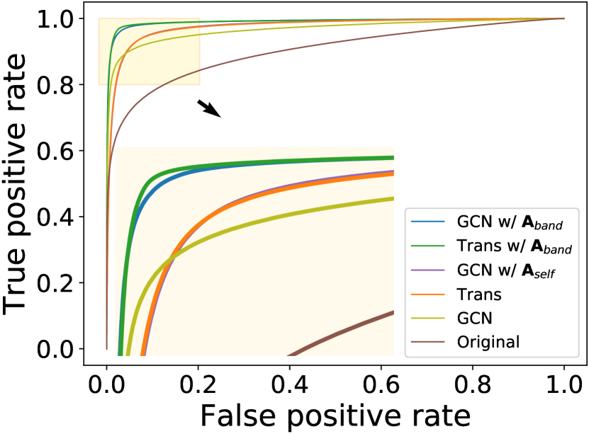
(a) MS-Celeb Part1

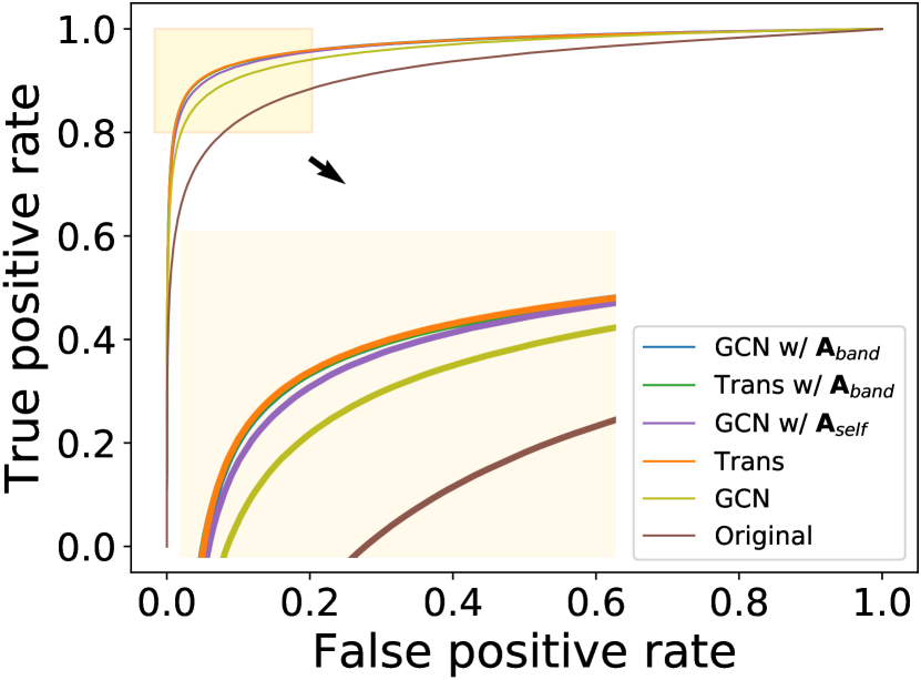
(b) MSMT17

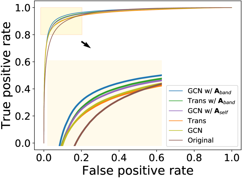
(c) VeRi-776

Figure 4: ROC curves of different methods on MS-Celeb Part1 (a), MSMT17 (b) and VeRi-776 (c).

3.4 Effectiveness of the downstream tasks

The improvement of graph structure learning can also be proven through the downstream tasks by exploiting the features it produces. The better the graph structure is learned, the better the performance on downstream tasks. Graphs have important applications in large-scale clustering and re-reranking in ReID. However, they suffer from inaccurate weight problems when learning and working with the graph structure. Armed the GCN with $\mathbf{A}_{band}$, many SOTA results are achieved.

Table 3: Clustering performance on MS-Celeb.

Dataset	Part1		Part3		Part5		Part7		Part9
Metrics	${F_{P}}$	${F_{B}}$	${F_{P}}$	${F_{B}}$	${F_{P}}$	${F_{B}}$	${F_{P}}$	${F_{B}}$	${F_{P}}$	${F_{B}}$
K-Means	79.21	81.23	73.04	75.20	69.83	72.34	67.90	70.57	66.47	69.42
HAC	70.63	70.46	54.40	69.53	11.08	68.62	1.40	67.69	0.37	66.96
DBSCAN	67.93	67.17	63.41	66.53	52.50	66.26	45.24	44.87	44.94	44.74
Clusformer	88.20	87.17	84.60	84.05	82.79	82.30	81.03	80.51	79.91	79.95
STAR-FC	91.97	90.21	88.28	86.26	86.17	84.13	84.70	82.63	83.46	81.47
Ada-NETS	92.79	91.40	89.33	87.98	87.50	86.03	85.40	84.48	83.99	83.28
Original+G-cut	69.63	73.62	63.31	66.56	60.61	62.91	57.13	58.72	54.42	58.54
Ours+G-cut	93.90	92.47	90.54	89.23	88.70	87.13	86.18	85.59	84.36	84.10
Original+Infomap	93.91	92.42	90.10	89.08	88.49	87.30	85.31	86.01	83.08	85.01
Ours+Infomap	94.94	93.67	91.74	90.81	89.50	89.15	87.04	87.81	85.40	86.76

Performance on clustering tasks

The clustering tasks are evaluated on MS-Celeb and MSMT17. Both of them have a large number of classes and are suitable as clustering benchmarks. The same features output by “GCN w/ $\mathbf{A}_{band}$” are used as that in Section A.3 for MS-Celeb and Section 3.3 for MSMT17. The same clustering method (denoted “G-cut”) is adopted as that in guo2020density ; wang2022adanets , where pairs of nodes are linked when their similarity scores are larger than a tuned threshold, and clustering is finally completed by transitively merging all links via a union-find algorithm anderson1991wait . The threshold is tuned for each dataset, aiming for the best balance between BCubed and Pairwise F-Scores. In addition, map equation based unsupervised clustering algorithm Infomap Rosvall2009 ; face-cluster-by-infomap is also adopted here. Their BCubed and Pairwise F-scores are listed in Table 3 and Table 10, where the results of current SOTA GCN/Transformer methods (Clusformer nguyen2021clusformer , STAR-FC shen2021starfc and Ada-NETS wang2022adanets ) and three conventional clustering approaches (K-Means lloyd1982least , HAC sibson1973slink and DBSCAN ester1996density ) are also listed. The results show that the features enhanced via our approach have the best clustering results in all datasets, either with G-cut or Infomap, both of which outperform the current SOTA methods Ada-NETS and STAR-FC with large margins. In comparison, the results of the ones with Infomap are better than those with G-cut.

Table 4: ReID performance on MSMT17 and VeRi-776.

Datasets	MSMT17		VeRi-776
Metrics	mAPR	R1	mAPR	R1
Original Feature	62.76	82.36	79.00	96.60
GCN	74.66	85.36	82.31	96.60
Transformer	77.60	86.37	82.62	96.54
GCN w/ $\mathbf{A}_{self}$	77.34	85.49	84.29	96.30
Trans w/ $\mathbf{A}_{band}$	77.49	86.54	83.98	96.72
GCN w/ $\mathbf{A}_{band}$	78.28	86.64	84.74	96.78
Original+QE	71.10	84.37	83.09	95.47
Original+LBR	70.36	85.28	83.63	97.13
Original+KR	76.46	85.48	82.32	96.84
Original+ECN	78.79	86.16	84.25	97.13

Performance on ReID tasks

The ReID tasks is evaluated on two ReID datasets: MSMT17 and VeRi-776. The enhanced features used are the same as those in Table 2. mAP^R and R1 are evaluated following the standard probe and gallery protocols of MSMT17 and VeRi-776. The results are shown in Table 4. As the output feature of learned graph can also be understood as a rerank process in ReID, comparisons are also made on commonly used rerank methods: QE chum2007total , LBR luo2019spectral , KR zhong2017re and ECN sarfraz2018pose . Table 4 shows that the “GCN w/ $\mathbf{A}_{band}$” achieves the best or comparable performance, and all enhanced features are much better than the original SOTA ones. In MSMT17, similar to the results in Section 3.3, the baselines with attention mechanism have very close performance, but work much better than the GCN. In VeRi-776, from the mAP^R perspective, $\mathcal{B}$-Attention works better than $\mathbf{A}_{self}$, and both of them are better than the GCN, but their R1 results are comparable. These results still support the superiority of the proposed approach, although R1 results of VeRi-776 are comparable, as mAP^R is a more comprehensive indication of feature quality for ReID. The experiments on the combination of “GCN w/ $\mathbf{A}_{band}$” with these commonly used rerank methods are also conducted in Section A.6, achieving more SOTA performances and proving the complementarity between them.

4 Related Work

Graph Convolutional Networks.

GCNs kipf2017semi ; hamilton2017inductive ; DBLP:conf/iclr/VelickovicCCRLB18 extends the operation of convolution from the grid-data (e.g. images, videos) to non-grid data which is more common in the real world. The classic GCN kipf2017semi is proposed based on the spectral theory and achieves promising results on citation network datasets: Citeseer, Cora and Pubmed sen2008collective . GraphSAGE hamilton2017inductive further extends GCNs from transductive framework to inductive framework and obtains better results. GAT DBLP:conf/iclr/VelickovicCCRLB18 introduces the attention mechanism in GCN, making it more expressive. Fast-GCN chen2018fastgcn interprets graph convolutions as integral transforms of embedding functions under probability measures, which not only is efficient for training but also generalizes well for inference. Some research works schlichtkrull2018modeling ; zhang2019heterogeneous ; hu2020heterogeneous ; wang2019heterogeneous ; ChenYiqiCRGCN also advance GCNs for relational data modeling. However, these GCNs are all investigated on relational datasets that have explicit graph structures. This work aims to extend the capacity of GCNs to work on datasets (e.g., image objects) which have no explicitly defined graph structures.

Graph Structure Learning.

The literature GNNBook2022 suggests that research on graph structure learning for GCNs can be roughly divided into discrete-based and weighted-based ones. Some discrete-based methods elinas2020variational ; Kazi2020DifferentiableGM ; ma2019flexible ; franceschi2019learning treat the graph structures as random distributions and sample binary adjacency matrices from them. Another way wang2022adanets constructs discrete graphs based on heuristic proxy objectiveness aiming for clean yet rich neighbours for each node. The binary matrices methods are difficult to optimize because of the gradient breakage, so such methods resort to variational inference (e.g., approaches in elinas2020variational ; ma2019flexible ), reinforcement learning (e.g., approaches in Kazi2020DifferentiableGM ) or optimization in stages (e.g., approaches in wang2022adanets ), which may lead to sub-optimal solutions. In addition, the parameter size of distributions franceschi2019learning can be very large (e.g., $\mathcal{O}(Nk)$ where $N$ is the number of nodes and $k$ is the number of neighbours for each node) and therefore not suitable for large datasets. The weighted-based methods chen2019graphflow ; chen2020reinforcement ; on2020cut ; yang2018glomo ; huang2020location ; chen2020iterative ; henaff2015deep ; li2018adaptive ; guo2020density ; nguyen2021clusformer , which are the focus of this paper, learn weighted adjacency matrices so that it can be optimized by SGD techniques robbins1951stochastic ; kiefer1952stochastic ; bottou2018optimization . The main difference between these works chen2019graphflow ; chen2020reinforcement ; on2020cut ; yang2018glomo ; huang2020location ; chen2020iterative ; henaff2015deep ; li2018adaptive is in the similarity measure, which can be classified into attention-based chen2019graphflow ; chen2020reinforcement ; on2020cut ; yang2018glomo ; huang2020location ; chen2020iterative and kernel-based henaff2015deep ; li2018adaptive roughly. To enhance the discriminatory power of the similarity measure, they have adopted various forms: adding learnable parameters chen2019graphflow ; huang2020location ; chen2020iterative , introducing nonlinearity chen2020reinforcement ; on2020cut ; yang2018glomo , Gaussian kernel functions henaff2015deep ; li2018adaptive or self-attention guo2020density ; nguyen2021clusformer ; vaswani2017attention ; Choi2020LearningTG etc. However, these methods are sensitive to the noise from feature representations, particular when each node is represented by a high dimensional vector, leading to the problem of inaccurate weights and vulnerable graph structure. This work aims to propose a multiple samples based similarity measure to improve the robustness of graph structure learning. Another approach uses the low-rank, sparsity and feature smoothness properties of the real-world graph to optimize the graph structure Jin2020GraphSL , but these priors are suitable for community networks rather than graph of image objects. Some work Johnson2020LearningGS learns to augment the given graph with new edges by reinforcement learning to improve the performance of downstream tasks, but existing noisy edges problem in graphs cannot be handled.

5 Conclusion

The problem of inaccurate edge weights is identified in graph structure learning, analysed from the perspective of noise in feature vectors, and handled based on several tests. A novel and robust similarity measure Sim-M is proposed, proven to be superior and verified in experiments. Then it is designed in an elegant matrix form, i.e., $\mathcal{B}$-Attention mechanism, to improve the graph structure quality in GCNs. The superiority and robustness of $\mathcal{B}$-Attention are validated by comprehensive experiments and achieve many SOTA results on clustering and ReID benchmarks.

Checklist

1. For all authors…

   1. Do the main claims made in the abstract and introduction accurately reflect the paper’s contributions and scope? [Yes] See abstract and Section 1.

   2. Did you describe the limitations of your work? [Yes] See Section B in Appendix.

   3. Did you discuss any potential negative societal impacts of your work? [Yes] See Section C in Appendix.

   4. Have you read the ethics review guidelines and ensured that your paper conforms to them? [Yes] We have read the ethics guidelines on the official website.

2. If you are including theoretical results…

   1. Did you state the full set of assumptions of all theoretical results? [Yes] See Section 2.2.

   2. Did you include complete proofs of all theoretical results? [Yes] See Section 2.2

3. If you ran experiments…

   1. Did you include the code, data, and instructions needed to reproduce the main experimental results (either in the supplemental material or as a URL)? [No] The code and the data are proprietary. The instructions is in Section 3.

   2. Did you specify all the training details (e.g., data splits, hyperparameters, how they were chosen)? [Yes] See in Section 3.1, paragraph of Network architectures and settings and the paragraphs describing the corresponding experiment in Section 3.3.

   3. Did you report error bars (e.g., with respect to the random seed after running experiments multiple times)? [No] Error bars are not reported because it would be too computationally expensive.

   4. Did you include the total amount of compute and the type of resources used (e.g., type of GPUs, internal cluster, or cloud provider)? [Yes] See Section A.7.

4. If you are using existing assets (e.g., code, data, models) or curating/releasing new assets…

   1. If your work uses existing assets, did you cite the creators? [Yes] See the Datasets paragraph in Section 3.1.

   2. Did you mention the license of the assets? [No] The used assets are very common in papers of computer vision.

   3. Did you include any new assets either in the supplemental material or as a URL? [No]

   4. Did you discuss whether and how consent was obtained from people whose data you’re using/curating? [No] The used assets are very common in papers of computer vision.

   5. Did you discuss whether the data you are using/curating contains personally identifiable information or offensive content? [Yes] See the footnote in Datasets paragraph in Section 3.1: Considering the ethical and privacy issues, all the datasets used in this paper are feature vectors which can not be restored to images.

5. If you used crowdsourcing or conducted research with human subjects…

   1. Did you include the full text of instructions given to participants and screenshots, if applicable? [N/A]

   2. Did you describe any potential participant risks, with links to Institutional Review Board (IRB) approvals, if applicable? [N/A]

   3. Did you include the estimated hourly wage paid to participants and the total amount spent on participant compensation? [N/A]

Appendix A Experiments

A.1 Details of the dataset

MS-Celeb guo2016ms is a dataset with 10M face images of nearly 100K individuals. A cleaned version deng2019arcface with about 5.8M face images of 86K identities is used in this paper. The protocol and features are the same as that in yang2019learning , where the dataset is divided into 10 parts by identities (Part0-9): Part0 for training and Part1-9 for testing. The feature dimension is 256. The data amounts of Part 0-9 (0, 1, 3, 5, 7 and 9) are respectively: 584K, 584K, 1.74M, 2.89M, 4.05M and 5.21M.

MSMT17 wei2018person is the current largest ReID dataset. It contains 32,621 images of 1,041 individuals for training and 93,820 images of 3,060 individuals for testing. These images are captured by 15 cameras under different time periods, weather and light conditions. This work uses the SOTA features from AGW pami21reidsurvey with a dimension of 2048.

VeRi-776 7553002 is a commonly used vehicle ReID benchmark, which contains over 40K bounding boxes of 619 vehicles captured by 20 cameras in unconstrained traffic scenes. The dataset is divided into two parts: 37,715 images of 576 vehicles for training, and 13,257 images of 200 vehicles for testing. This work uses the features extracted by the SOTA ViT-B/16 Baseline in TransReID He_2021_ICCV , with 768 dimensions.

A.2 Effectiveness of the Sim-M

The experiments on MSMT17 and VeRi-776 also show that the advantage of Sim-M over Sim-S is increasingly obvious as $k$ increases and then drops for introduction of too much noise as in Table 5.

Table 5: AUC of Sim-S (AUC_S), Sim-M (AUC_M) and their difference (AUC_δ=AUC_M-AUC_S) on MSMT17 and VeRi-776. The values of AUC are scaled by a factor of 100 for a better show.

Datasets	MSMT17				VeRi-776
$k$	ENR	AUCS	AUCM	AUCδ	ENR	AUCS	AUCM	AUCδ
5	0.06	89.23	89.74	0.52	0.01	90.96	90.40	-0.56
10	0.13	89.33	90.02	0.69	0.03	89.34	90.09	0.75
20	0.26	87.78	88.63	0.85	0.07	85.86	86.54	0.68
40	0.48	86.72	86.62	-0.10	0.17	83.05	82.89	-0.16

A.3 Performance on larger scales of MS-Celeb

Experiments are also conducted to compare these baselines on larger scales of MS-Celeb (i.e., Part3-9). The same model for MS-Celeb Part1 is used as in Section 3.3, but tested on Part3-9. The results in Table 6 show that all baselines have performance degradation when the scale enlarges. The $\mathcal{B}$-Attention obtains the best results in all parts; $\mathbf{A}_{self}$ works better than GCN; all output features are much better than the original ones. Among the baselines with attention mechanisms, the ones using GCN-based networks have better performances. The GCN with $\mathbf{A}_{band}$ has the highest mAP scores. Figure 5 shows the ROC curves of GCN, “GCN w/ $\mathbf{A}_{self}$” and “GCN w/ $\mathbf{A}_{band}$” across all parts of MS-Celeb, from which we can also see the performance degradation with larger testsets. The performance degradation of “GCN w/ $\mathbf{A}_{band}$” is much smaller than the other two baselines, which is shown more clearly from the differences of AUC in Table 7. In Table 7, differences on AUC of two adjacent parts  (e.g., part1 - part3, part3 - part5, part5 - part7, part7 - part9) and their summation for each method are shown. It can be observed that the summation of the differences of “GCN w/ $\mathbf{A}_{band}$” is 1.49, which is only 58.30% and 67.26% of the ones of GCN (2.56) and “GCN with $\mathbf{A}_{self}$" (2.22). This validates that the features from “GCN w/ $\mathbf{A}_{band}$” have a much smaller performance degradation than the other two baselines with larger testsets from the perspective of verification. Similar observations can also be seen in Table 6, where the performance degradation of the baselines with attention mechanisms is much smaller than GCN and original features.

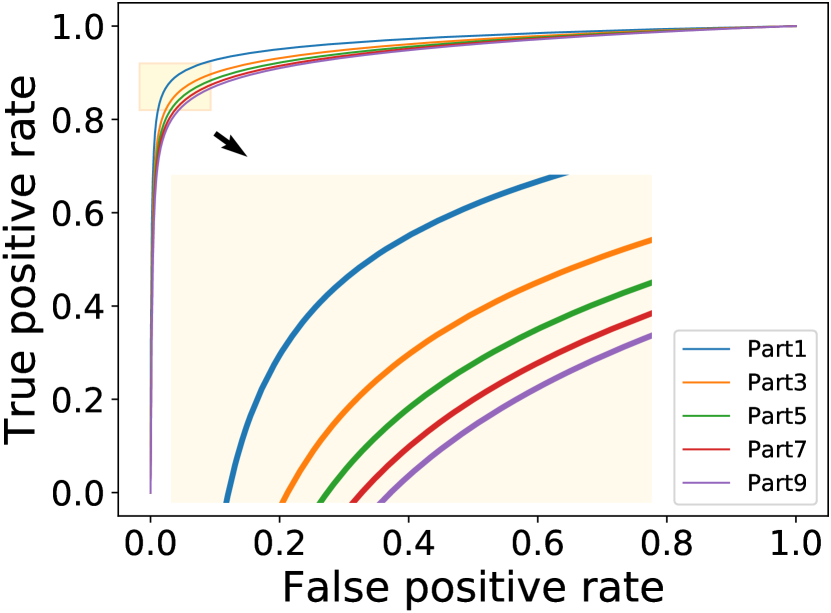
(a) GCN

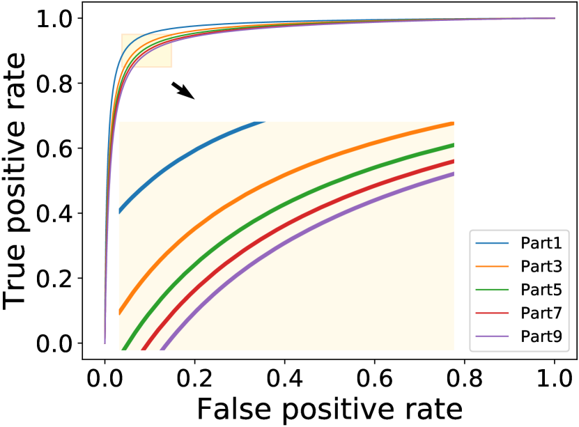
(b) GCN with $\mathbf{A}_{self}$

(c) GCN with $\mathbf{A}_{band}$

Figure 5: ROC curves of GCN (a), GCN with $\mathbf{A}_{self}$ (b), and GCN with $\mathbf{A}_{band}$ (c) on MS-Celeb Part1-9.

Table 6: Feature quality (mAP) on different scales of MS-Celeb.

Partition	Part1	Part3	Part5	Part7	Part9
Original Feature	80.07	75.28	73.21	71.73	70.63
GCN	90.15	86.27	84.34	82.95	81.90
Transformer	93.86	91.32	89.99	89.03	88.28
GCN w/ $\mathbf{A}_{self}$	94.09	91.66	90.38	89.45	88.73
Trans w/ $\mathbf{A}_{band}$	95.70	93.38	92.08	91.09	90.30
GCN w/ $\mathbf{A}_{band}$	95.97	93.71	92.38	91.30	90.46

Table 7: Differences on AUC ($\delta_{AUC}$) of two adjacent parts of MS-Celeb for GCN, “GCN with $\mathbf{A}_{self}$" and “GCN with $\mathbf{A}_{band}$". The values in the table are scaled by a factor of 100 for better display.

$\delta_{AUC}$	GCN	GCN with $\mathbf{A}_{self}$	GCN with $\mathbf{A}_{band}$
part1 - part3	1.23	1.03	0.58
part3 - part5	0.58	0.51	0.37
part5 - part7	0.43	0.37	0.30
part7 - part9	0.32	0.31	0.25
summation	2.56	2.22	1.49

A.4 Ablation study on $\mathcal{B}$-Attention

Ablation experiments are conducted mainly on MS-Celeb to study the design of the topological architecture and attention fusion method of $\mathcal{B}$-Attention. Similar to Section 3.3, models are trained on Part0 and tested on Part1. All settings other than the factor being investigated are the same as that in Section 3.3 for “GCN with $\mathbf{A}_{band}$” with $k=120$.

A.4.1 topological architecture design

This study compares the topological architecture of the $\mathcal{B}$-Attention with three other designs: (1) one with only the $\mathbf{A}_{qart}$ of $\mathcal{B}$-Attention; (2) one using only the $\mathcal{Q}$-Attention part but with the $\mathbf{A}_{X}$ replaced by $\mathbf{A}_{self}$ in Equation 8, denoted as $\widetilde{\mathbf{A}}_{qart}$; (3) and one with $\mathcal{B}$-Attention but with the $\mathbf{A}_{qart}$ replaced by $\widetilde{\mathbf{A}}_{qart}$, denoted as $\widetilde{\mathbf{A}}_{band}$. Table 8 shows their mAP results, where the results of “GCN w/ $\mathbf{A}_{band}$” and one with only $\mathbf{A}_{self}$ are also listed for comparison. For the purpose of ablation study, the one with only $\mathbf{A}_{self}$ here has the same depth (i.e., three layers) with “GCN w/ $\mathbf{A}_{band}$”, which is different from that in Table 2 (two layers). The comparisons are made on two conditions: with or without $\mathbf{W}_{qart}$ (i.e., $\mathbf{W}^{Q}_{qart}$ and $\mathbf{W}^{K}_{qart}$) in Equation 8. For the cases without $\mathbf{W}_{qart}$, $\mathbf{W}^{Q}_{qart}$ and $\mathbf{W}^{K}_{qart}$ are both identity matrices, i.e., $\mathbf{Q}_{qart}=\mathbf{K}_{qart}=\mathbf{A}_{X}$. Their ROC curves are shown in Figure 6. It can be seen that the $\mathcal{B}$-Attention design achieves the best results in both mAP and ROC; $\mathbf{A}_{qart}$ has better performance than $\mathbf{A}_{self}$; $\widetilde{\mathbf{A}}_{qart}$ and $\widetilde{\mathbf{A}}_{band}$ are worse than $\mathbf{A}_{qart}$ and $\mathbf{A}_{band}$ respectively. This shows that the combination of $\mathbf{A}_{self}$ and $\mathbf{A}_{qart}$ and the use of $\mathbf{A}_{X}$ (instead of $\mathbf{A}_{self}$) in $\mathbf{A}_{qart}$ both contribute to the performance improvement. In addition, the baselines with $\mathbf{W}_{qart}$ have better performances (higher mAP scores and better ROC) than those without, indicating that $\mathbf{W}^{Q}_{qart}$ and $\mathbf{W}^{K}_{qart}$ are also critical for better graph structure learning.

Table 8: Feature quality (mAP) of different topological architectures of the attention mechanism.

Arch./Cond.	w/ $\mathbf{W}_{qart}$	w/o $\mathbf{W}_{qart}$
$\mathbf{A}_{self}$	88.10	88.10
$\widetilde{\mathbf{A}}_{qart}$	90.10	89.40
$\mathbf{A}_{qart}$	92.26	88.92
$\widetilde{\mathbf{A}}_{band}$	94.19	89.53
$\mathbf{A}_{band}$	95.97	93.67

Figure 6: ROC curves of different topological architectures of the attention mechanism.

The ablation experiments are also conducted on attention map fusion method in Section A.4.2 in Appendix. The results in Table 9 and Figure 7 together will prove that the proposed form in Equation 11 has the best performance across all datasets.

A.4.2 Attention map fusion method

The attention map fusion method is studied by comparing it to two other designs: direct element-wise addition without weighting ($\mathbf{A}_{qart}+\mathbf{A}_{self}$) and element-wise multiplication ($\mathbf{A}_{qart}\odot\mathbf{A}_{self}$) in Equation 11. The results are shown in Table 9 and Figure 7: The $\theta_{qart}\mathbf{A}_{qart}+\theta_{self}\mathbf{A}_{self}$ design works the best, and the performance of $\mathbf{A}_{qart}\odot\mathbf{A}_{self}$ is very close to $\theta_{qart}\mathbf{A}_{qart}+\theta_{self}\mathbf{A}_{self}$. However, results of MSMT17 and VeRi-776 in Table 9 shows our proposed method has the best performance across all datasets.

Table 9: Feature quality (mAP) of different attention map fusion methods, where $\odot$ denotes element-wise multiplication.

Dataset	$\mathbf{A}_{qart}+\mathbf{A}_{self}$	$\mathbf{A}_{qart}\odot\mathbf{A}_{self}$	$\theta_{qart}\mathbf{A}_{qart}+\theta_{self}\mathbf{A}_{self}$
MS-Celeb	92.83	95.71	95.97
MSMT17	84.95	85.59	86.04
VeRi-776	85.97	85.53	87.59

Figure 7: ROC curves of different fusion methods on MS-Celeb (part1).

Table 10: Clustering performance on MSMT17.

Dataset	MSMT17
Metrics	${F_{P}}$	${F_{B}}$
K-Means	60.32	69.28
HAC	63.95	73.75
DBSCAN	48.23	53.90
Clusformer	-	-
STAR-FC	-	-
Ada-NETS	73.51	77.40
Original+G-cut	50.60	66.56
Ours+G-cut	74.93	79.91
Original+Infomap	71.33	79.16
Ours+Infomap	77.54	81.75

A.5 Clustering performance on MSMT17

The clustering tasks are also evaluated on MSMT17 and the results are in Table 10.

A.6 Ensemble Performance on ReID tasks

In addition to directly comparing with the commonly used rerank methods (e.g., QE chum2007total , LBR luo2019spectral , KR zhong2017re and ECN sarfraz2018pose ) in Section 4.4, the “GCN with $\mathbf{A}_{band}$" can also be combined with them. The commonly used rerank methods can utilize the enhanced features from “GCN with $\mathbf{A}_{band}$" for better ranking. The results are shown in Table 11. Since mAP^R can provide a more comprehensive evaluation of the feature quality than R1 for ReID, the mAP^R is discussed more often. It can be observed that new SOTA performances are obtained on both datasets. The mAP^R on MSMT17 is as high as 79.67 by “$\mathbf{A}_{band}$+KR" and on VeRi-776 is as high as 85.92 by “$\mathbf{A}_{band}$+LBR". For most of the commonly used rerank methods, the mAP^R of reranking with $\mathbf{A}_{band}$ is higher than with original features and also higher than “GCN w/ $\mathbf{A}_{band}$”. The only exception is “$\mathbf{A}_{band}$+ECN" which is higher than “GCN w/ $\mathbf{A}_{band}$” but only comparable with “original+ECN". The results show that there is a complementary relationship between “GCN with $\mathbf{A}_{band}$" and commonly used rerank methods. The “GCN with $\mathbf{A}_{band}$" can provide better features so that the commonly used rerank methods can be further improved, although the ${R1}$ results are only comparable.

Table 11: Ensemble ReID performance on MSMT17 and VeRi-776. “Original+X" means reranking with original features by methods of “X". “$\mathbf{A}_{band}$+X" means reranking with features from “GCN w/ $\mathbf{A}_{band}$" by methods of “X".

Dataset	MSMT17		VeRi-776
Metrics	mAPR	R1	mAPR	R1
Original Feature	62.76	82.36	79.00	96.60
GCN w/ $\mathbf{A}_{band}$	78.28	86.64	84.74	96.78
Original+QE	71.10	84.37	83.09	95.47
Original+LBR	70.36	85.28	83.63	97.13
Original+KR	76.46	85.48	82.32	96.84
Original+ECN	78.79	86.16	84.25	97.13
$\mathbf{A}_{band}$+QE	79.37	86.91	85.88	96.90
$\mathbf{A}_{band}$+LBR	79.54	86.86	85.92	96.90
$\mathbf{A}_{band}$+KR	79.67	84.81	85.45	96.60
$\mathbf{A}_{band}$+ECN	78.70	84.05	85.61	96.90

A.7 Declaration of the type of computing resources

All experiments are conducted on a single machine, with 54 E5-2682 v4 CPUs, 8 NVIDIA P100 cards and 400G memory.

Appendix B Limitations

Our approach achieves promising results in graph structure learning, but it still has the following limitations:

• The $\mathcal{B}$-Attention requires more computation and number of parameters as shown in Section 2.3. However, the baseline methods can not achieve the same performance even adding their network depth. The layer number of network in each method is tuned in all experiments.

• The superiority of $\mathcal{B}$-Attention is not obvious enough on datasets with few samples in each category compared with self attention as revealed in Section  3.3.

• The performance of $\mathcal{B}$-Attention will also degrade when with large ENR as discussed in Section 3.3, indicating the current form still has improvement room on the robustness against noise to further investigate.

• The outputs $\mathcal{B}$-Attention will vary depending on the choice of nearest neighbours. However, the superiority of this method can be guaranteed as long as the conditions in Section 2.2 are met.

Appendix C Potential Negative Societal Impacts

The proposed graph structure learning method inherently is harmless just like many other AI technologies. This technology may have negative societal impacts if someone uses it for malicious applications such as surveillance, personal information collections. As authors, we advocate for proper technology usage.

Appendix D Pseudocode for self-attention and $\mathcal{Q}$-Attention

Algorithm 1 PyTorch-style pseudocode for self-attention and $\mathcal{Q}$-Attention

⬇

# X: the input feature matrix, with shape (N, D)

def self_attention(X):

Q_self = torch.matmul(X, W_self_Q)

K_self = torch.matmul(X, W_self_K)

self_attn = torch.matmul(Q_self, K_self.transpose(-2, -1))

return self_attn

def Q_attention(X):

A_X = torch.matmul(X, X.transpose(-2, -1))

Q_qart = torch.matmul(A_X, W_qart_Q)

K_qart = torch.matmul(A_X, W_qart_K)

Q_attn = torch.matmul(Q_qart, K_qart.transpose(-2, -1))

return Q_attn

Appendix E Detailed Proof of with generalized version of Chernoff Bounds

Below is a full analysis for the practical algorithm in Section 2.3 that does not assume a binary relationship between two nodes in $A_{X}$.

Let $X_{i}$ denote a random variable with no distribution assumptions such that $a\leq X_{i}\leq b$ for all $i$. Define $X=\sum_{1}^{m}X_{i}$, $\mu=\mathbb{E}(X)$. Then for all $0<\epsilon<1$, we have the general version of Chernoff inequality as follows.

$(i)\ \ \textbf{Upper Tail:}\ \ \mathbb{P}(X\geq(1+\epsilon)\mu)\leq e^{-\frac{\epsilon^{2}\mu^{2}}{m(b-a)^{2}}}\$;

$(ii)\ \ \textbf{Lower Tail:}\ \ \mathbb{P}(X\leq(1-\epsilon)\mu)\leq e^{-\frac{\epsilon^{2}\mu^{2}}{m(b-a)^{2}}}$ .

The above show that with probability at least $1-\delta$, $(1-\epsilon)\mu\leq X\leq(1+\epsilon)\mu$ where $\delta=e^{-\frac{\epsilon^{2}\mu^{2}}{m(b-a)^{2}}}$ or equivalently $\epsilon=\sqrt{\frac{m(b-a)^{2}log(1/\delta)}{\mu^{2}}}$.

Instead of assuming $p$ and $q$ for making connections in the case of $C(v_{i})=C(v_{j})$ and $C(v_{i})\neq C(v_{j})$, we assume that the similarity score $s_{i,j}$ is sampled from a bounded distribution (bounded between -1 and +1) with mean of $s_{+}$ when $C(v_{i})=C(v_{j})$, and $s_{i,j}$ is sampled from a bounded distribution (bound between -1 and +1) with mean of $s_{-}$ when $C(v_{i})=C(v_{j})$. We of course assume $s_{+}>s_{-}$. In expectation, the number of edges connected under $S_{i,j}^{k}$ on $\mathcal{V}_{i,j}$ is

$$\left\{\begin{array}[]{ll}\mu^{-}=s_{+}s_{-}m,&C(v_{i})\neq C(v_{j})\ ,\\ \mu^{+}=(\alpha s_{+}^{2}+(1-\alpha)s_{-}^{2})m,&C(v_{i})=C(v_{j})\ ,\end{array}\right.$$ (12)

where $C(v)$ is the category of node $v$.

It should be noted that $(b-a)^{2}=4$ under our assumption. Therefore, when $v_{i},v_{j}$ are sampled from different categories, we have, with probability at least $1-\delta$,

$$\sum_{k\in V_{i,j}}S_{i,j}^{k} \leq(1+\epsilon^{-})\mu^{-}$$ (13)

$$\sum_{k\in V_{i,j}}S_{i,j}^{k} \leq\left(1+\sqrt{\frac{4mlog(1/\delta)}{(\mu^{-})^{2}}}\right)\mu^{-}$$

$$S_{i,j}=\frac{1}{m}\sum_{k\in V_{i,j}}S_{i,j}^{k} \leq\left(1+\sqrt{\frac{4nlog(1/\delta)}{(s_{+}s_{-}m)^{2}}}\right)s_{+}s_{-}\ .$$

When $v_{i},v_{j}$ are sampled from the same category, we have, with probability at least $1-\delta$,

$$\sum_{k\in V_{i,j}}S_{i,j}^{k} \geq(1-\epsilon^{+})\mu^{+}$$ (14)

$$\sum_{k\in V_{i,j}}S_{i,j}^{k} \geq\left(1-\sqrt{\frac{4mlog({1/\delta})}{\mu^{+}}}\right)\mu^{+}$$

$$S_{i,j}=\frac{1}{m}\sum_{k\in V_{i,j}}S_{i,j}^{k} \geq\left(1-\sqrt{\frac{4nlog(1/\delta)}{(\alpha s_{+}^{2}+(1-\alpha)s_{-}^{2})^{2}m^{2}}}\right)(\alpha s_{+}^{2}+(1-\alpha)s_{-}^{2})\ .$$

The two distributions can be well separated if the above two bounds do not overlap. That is, we require that

$$(1+\epsilon^{-})\mu^{-}<(1-\epsilon^{+})\mu^{+}\ .$$ (15)

On the other hand, it is obvious $s_{+}s_{-}<\alpha s_{+}^{2}+(1-\alpha)s_{-}^{2}$, so we know

$$\epsilon^{-}=\sqrt{\frac{4mlog(1/\delta)}{(s_{+}s_{-}m)^{2}}}>\epsilon^{+}=\sqrt{\frac{4mlog(1/\delta)}{(\alpha s_{+}^{2}+(1-\alpha)s_{-}^{2})^{2}m^{2}}}\ .$$ (16)

Set $\epsilon=\epsilon^{-}$ to have a larger step and a stricter condition, we have

$$(1+\epsilon)\mu^{-} <(1-\epsilon)\mu^{+}$$ (17)

$$\epsilon <\frac{u^{+}-u^{-}}{u^{+}+u^{-}}$$

$$\sqrt{\frac{4m\log{(1/\delta)}}{(s_{+}s_{-}m)^{2}}}<\frac{(s_{+}-s_{-})^{2}+(2\alpha-1)(s_{+}^{2}-s_{-}^{2})}{(s_{+}+s_{-})^{2}+(2\alpha-1)(s_{+}^{2}-s_{-}^{2})}.$$ (18)

Because $\alpha>\frac{1}{2}$ and $s_{+}>s_{-}$,

$$(s_{+}-s_{-})^{2}+(2\alpha-1)(s_{+}^{2}-s_{-}^{2}) >0,$$ (19)

$$(s_{+}+s_{-})^{2}+(2\alpha-1)(s_{+}^{2}-s_{-}^{2}) >0.$$

So we have

$$m>\frac{4((s_{+}+s_{-})^{2}+(2\alpha-1)(s_{+}^{2}-s_{-}^{2}))^{2}}{s_{+}^{2}s_{-}^{2}((s_{+}-s_{-})^{2}+(2\alpha-1)(s_{+}^{2}-s_{-}^{2}))^{2}})\log(\frac{1}{\delta}).$$ (20)

We complete the proof by substituting $\delta$ with

$$\delta\triangleq\frac{1}{\gamma}\min((1-\alpha)s_{-},\alpha(1-s_{+})).$$ (21)

where $\gamma>1$ is a constant.

Finally, we prove that

$$m>\frac{4((s_{+}+s_{-})^{2}+(2\alpha-1)(s_{+}^{2}-s_{-}^{2}))^{2}}{s_{+}^{2}s_{-}^{2}((s_{+}-s_{-})^{2}+(2\alpha-1)(s_{+}^{2}-s_{-}^{2}))^{2}}\log\left(\frac{\gamma}{\min((1-\alpha)s_{-},\alpha(1-s_{+}))}\right)\ .$$ (22)

We can guarantee that when the above condition is met, the proposed similarity measure between two nodes from the same category is strictly larger than that for two nodes from different categories. It is able to reduce the number of noisy edges and missing edges of the single test method by $1/\gamma$ in expectation.

Appendix F Case Studies on self attention, $\mathcal{Q}$-Attention and $\mathcal{B}$-Attention

To better understand the effect of multiple tests (i.e. the fourth order of statistics), we illustrate the effect of self-attention, $\mathcal{Q}$-Attention and $\mathcal{B}$-Attention with the help of the tool BertViz.

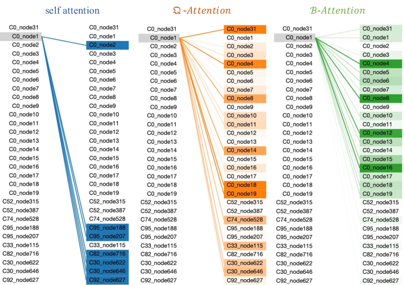
Figure 8: Case studies on self attention, $\mathcal{Q}$-Attention and $\mathcal{B}$-Attention. Each entry contains the category and node index, e.g. “C0_node1” means this node belongs to category 0 and the node index is 1. The shade of the colour represents the weight of attention. The darker the colour, the greater the weight. The data of this case is sampled from the last layer of $\mathcal{B}$-Attention on the MS-Celeb part1.

As shown in the left panel of Figure 8, self-attention introduces a number of noisy connections between nodes belonging to different categories. In contrast, according to the middle panel of Figure 8, $\mathcal{Q}\textbf{-Attention}$ is able to introduce many more connections between nodes from the same category, and at the same time significantly reduces the weights for those noisy connections. In the last panel, the combination self-attention with the fourth order statistics, The $\mathcal{B}\textbf{-Attention}$ further removes those noisy connections while keeps most of the clean connections between nodes.

References

- [1] Enrique Amigó, Julio Gonzalo, Javier Artiles, and Felisa Verdejo. A comparison of extrinsic clustering evaluation metrics based on formal constraints. Information retrieval, 12(4):461–486, 2009.
- [2] Richard J Anderson and Heather Woll. Wait-free parallel algorithms for the union-find problem. In Proceedings of the twenty-third annual ACM symposium on Theory of computing, pages 370–380, 1991.
- [3] Amit Bagga and Breck Baldwin. Algorithms for scoring coreference chains. In The first international conference on language resources and evaluation workshop on linguistics coreference, volume 1, pages 563–566. Citeseer, 1998.
- [4] Irénée-Jules Bienaymé. Considérations à l’appui de la découverte de Laplace sur la loi de probabilité dans la méthode des moindres carrés. Imprimerie de Mallet-Bachelier, 1853.
- [5] Léon Bottou, Frank E Curtis, and Jorge Nocedal. Optimization methods for large-scale machine learning. Siam Review, 60(2):223–311, 2018.
- [6] Jie Chen, Tengfei Ma, and Cao Xiao. Fastgcn: fast learning with graph convolutional networks via importance sampling. In International conference on learning representations (ICLR), 2018.
- [7] Yiqi Chen, Tieyun Qian, Wanli Li, and Yile Liang. Exploiting composite relation graph convolution for attributed network embedding. Journal of Computer Research and Development, pages 1674–1682, 2020.
- [8] Yu Chen, Lingfei Wu, and Mohammed Zaki. Iterative deep graph learning for graph neural networks: Better and robust node embeddings. Advances in Neural Information Processing Systems, 33:19314–19326, 2020.
- [9] Yu Chen, Lingfei Wu, and Mohammed J Zaki. Graphflow: Exploiting conversation flow with graph neural networks for conversational machine comprehension. arXiv preprint arXiv:1908.00059, 2019.
- [10] Yu Chen, Lingfei Wu, and Mohammed J Zaki. Reinforcement learning based graph-to-sequence model for natural question generation. In International conference on learning representations (ICLR), 2020.
- [11] Herman Chernoff. A measure of asymptotic efficiency for tests of a hypothesis based on the sum of observations. The Annals of Mathematical Statistics, pages 493–507, 1952.
- [12] E. Choi, Zhen Xu, Yujia Li, Michael W. Dusenberry, Gerardo Flores, Yuan Xue, and Andrew M. Dai. Learning the graphical structure of electronic health records with graph convolutional transformer. In AAAI, 2020.
- [13] Ondrej Chum, James Philbin, Josef Sivic, Michael Isard, and Andrew Zisserman. Total recall: Automatic query expansion with a generative feature model for object retrieval. In 2007 IEEE 11th International Conference on Computer Vision, pages 1–8, Rio de Janeiro, Brazil, 2007. IEEE.
- [14] Thomas Cover and Peter Hart. Nearest neighbor pattern classification. IEEE transactions on information theory, 13(1):21–27, 1967.
- [15] Jiankang Deng, Jia Guo, Niannan Xue, and Stefanos Zafeiriou. Arcface: Additive angular margin loss for deep face recognition. In Proceedings of the IEEE/CVF Conference on Computer Vision and Pattern Recognition, pages 4690–4699, 2019.
- [16] Pantelis Elinas, Edwin V Bonilla, and Louis Tiao. Variational inference for graph convolutional networks in the absence of graph data and adversarial settings. Advances in Neural Information Processing Systems, 33:18648–18660, 2020.
- [17] Martin Ester, Hans-Peter Kriegel, Jörg Sander, Xiaowei Xu, et al. A density-based algorithm for discovering clusters in large spatial databases with noise. In Kdd, volume 96, pages 226–231, 1996.
- [18] Luca Franceschi, Mathias Niepert, Massimiliano Pontil, and Xiao He. Learning discrete structures for graph neural networks. In International conference on machine learning, pages 1972–1982. PMLR, 2019.
- [19] Xavier Glorot, Antoine Bordes, and Yoshua Bengio. Deep sparse rectifier neural networks. In Proceedings of the fourteenth international conference on artificial intelligence and statistics, pages 315–323. JMLR Workshop and Conference Proceedings, 2011.
- [20] Senhui Guo, Jing Xu, Dapeng Chen, Chao Zhang, Xiaogang Wang, and Rui Zhao. Density-aware feature embedding for face clustering. In Proceedings of the IEEE/CVF Conference on Computer Vision and Pattern Recognition, pages 6698–6706, 2020.
- [21] Yandong Guo, Lei Zhang, Yuxiao Hu, Xiaodong He, and Jianfeng Gao. Ms-celeb-1m: A dataset and benchmark for large-scale face recognition. In European conference on computer vision, pages 87–102. Springer, 2016.
- [22] William L Hamilton, Rex Ying, and Jure Leskovec. Inductive representation learning on large graphs. arXiv preprint arXiv:1706.02216, 2017.
- [23] Kaiming He, Xiangyu Zhang, Shaoqing Ren, and Jian Sun. Delving deep into rectifiers: Surpassing human-level performance on imagenet classification. In Proceedings of the IEEE international conference on computer vision, pages 1026–1034, 2015.
- [24] Shuting He, Hao Luo, Pichao Wang, Fan Wang, Hao Li, and Wei Jiang. Transreid: Transformer-based object re-identification. In Proceedings of the IEEE/CVF International Conference on Computer Vision (ICCV), pages 15013–15022, October 2021.
- [25] Mikael Henaff, Joan Bruna, and Yann LeCun. Deep convolutional networks on graph-structured data. arXiv preprint arXiv:1506.05163, 2015.
- [26] Wassily Hoeffding. On the distribution of the number of successes in independent trials. The Annals of Mathematical Statistics, pages 713–721, 1956.
- [27] Ziniu Hu, Yuxiao Dong, Kuansan Wang, and Yizhou Sun. Heterogeneous graph transformer. In Proceedings of The Web Conference 2020, pages 2704–2710, 2020.
- [28] Deng Huang, Peihao Chen, Runhao Zeng, Qing Du, Mingkui Tan, and Chuang Gan. Location-aware graph convolutional networks for video question answering. In Proceedings of the AAAI Conference on Artificial Intelligence, volume 34, pages 11021–11028, 2020.
- [29] Wei Jin, Yao Ma, Xiaorui Liu, Xianfeng Tang, Suhang Wang, and Jiliang Tang. Graph structure learning for robust graph neural networks. Proceedings of the 26th ACM SIGKDD International Conference on Knowledge Discovery & Data Mining, 2020.
- [30] Daniel D. Johnson, H. Larochelle, and Daniel Tarlow. Learning graph structure with a finite-state automaton layer. In Advances in Neural Information Processing Systems, 2020.
- [31] Anees Kazi, Luca Di Cosmo, Nassir Navab, and Michael M. Bronstein. Differentiable graph module (dgm) graph convolutional networks. ArXiv, abs/2002.04999, 2020.
- [32] Michael J Kearns and Umesh Vazirani. An introduction to computational learning theory. MIT press, 1994.
- [33] Jack Kiefer, Jacob Wolfowitz, et al. Stochastic estimation of the maximum of a regression function. The Annals of Mathematical Statistics, 23(3):462–466, 1952.
- [34] Thomas N. Kipf and Max Welling. Semi-supervised classification with graph convolutional networks. In International Conference on Learning Representations (ICLR), 2017.
- [35] Ruoyu Li, Sheng Wang, Feiyun Zhu, and Junzhou Huang. Adaptive graph convolutional neural networks. In Proceedings of the AAAI Conference on Artificial Intelligence, volume 32, 2018.
- [36] Shangqing Liu, Yu Chen, Xiaofei Xie, Jingkai Siow, and Yang Liu. Retrieval-augmented generation for code summarization via hybrid gnn. arXiv preprint arXiv:2006.05405, 2020.
- [37] Xinchen Liu, Wu Liu, Huadong Ma, and Huiyuan Fu. Large-scale vehicle re-identification in urban surveillance videos. In 2016 IEEE International Conference on Multimedia and Expo (ICME), pages 1–6, 2016.
- [38] Stuart Lloyd. Least squares quantization in pcm. IEEE transactions on information theory, 28(2):129–137, 1982.
- [39] Chuanchen Luo, Yuntao Chen, Naiyan Wang, and Zhaoxiang Zhang. Spectral feature transformation for person re-identification. In Proceedings of the IEEE International Conference on Computer Vision, pages 4976–4985, 2019.
- [40] Jiaqi Ma, Weijing Tang, Ji Zhu, and Qiaozhu Mei. A flexible generative framework for graph-based semi-supervised learning. Advances in Neural Information Processing Systems, 32, 2019.
- [41] Rajeev Motwani and Prabhakar Raghavan. Randomized algorithms. Cambridge university press, 1995.
- [42] Xuan-Bac Nguyen, Duc Toan Bui, Chi Nhan Duong, Tien D Bui, and Khoa Luu. Clusformer: A transformer based clustering approach to unsupervised large-scale face and visual landmark recognition. In Proceedings of the IEEE/CVF Conference on Computer Vision and Pattern Recognition, pages 10847–10856, 2021.
- [43] Kyoung-Woon On, Eun-Sol Kim, Yu-Jung Heo, and Byoung-Tak Zhang. Cut-based graph learning networks to discover compositional structure of sequential video data. In Proceedings of the AAAI Conference on Artificial Intelligence, volume 34, pages 5315–5322, 2020.
- [44] Herbert Robbins and Sutton Monro. A stochastic approximation method. The annals of mathematical statistics, pages 400–407, 1951.
- [45] Lorenzo Rosasco, Ernesto De Vito, Andrea Caponnetto, Michele Piana, and Alessandro Verri. Are loss functions all the same? Neural computation, 16(5):1063–1076, 2004.
- [46] M. Rosvall, D. Axelsson, and C. T. Bergstrom. The map equation. The European Physical Journal Special Topics, 178(1):13–23, 2009.
- [47] M Saquib Sarfraz, Arne Schumann, Andreas Eberle, and Rainer Stiefelhagen. A pose-sensitive embedding for person re-identification with expanded cross neighborhood re-ranking. In Proceedings of the IEEE Conference on Computer Vision and Pattern Recognition, pages 420–429, 2018.
- [48] Michael Schlichtkrull, Thomas N Kipf, Peter Bloem, Rianne van den Berg, Ivan Titov, and Max Welling. Modeling relational data with graph convolutional networks. In European semantic web conference, pages 593–607. Springer, 2018.
- [49] Prithviraj Sen, Galileo Namata, Mustafa Bilgic, Lise Getoor, Brian Galligher, and Tina Eliassi-Rad. Collective classification in network data. AI magazine, 29(3):93–93, 2008.
- [50] Shuai Shen, Wanhua Li, Zheng Zhu, Guan Huang, Dalong Du, Jiwen Lu, and Jie Zhou. Structure-aware face clustering on a large-scale graph with 107 nodes. In Proceedings of the IEEE Conference on Computer Vision and Pattern Recognition, 2021.
- [51] Yichun Shi, Charles Otto, and Anil K Jain. Face clustering: representation and pairwise constraints. IEEE Transactions on Information Forensics and Security, 13(7):1626–1640, 2018.
- [52] Robin Sibson. Slink: an optimally efficient algorithm for the single-link cluster method. The computer journal, 16(1):30–34, 1973.
- [53] Ashish Vaswani, Noam Shazeer, Niki Parmar, Jakob Uszkoreit, Llion Jones, Aidan N Gomez, Łukasz Kaiser, and Illia Polosukhin. Attention is all you need. Advances in neural information processing systems, 30, 2017.
- [54] Petar Velickovic, Guillem Cucurull, Arantxa Casanova, Adriana Romero, Pietro Liò, and Yoshua Bengio. Graph attention networks. In 6th International Conference on Learning Representations, ICLR 2018, Vancouver, BC, Canada, April 30 - May 3, 2018, Conference Track Proceedings. OpenReview.net, 2018.
- [55] Minjie Wang, Da Zheng, Zihao Ye, Quan Gan, Mufei Li, Xiang Song, Jinjing Zhou, Chao Ma, Lingfan Yu, Yu Gai, Tianjun Xiao, Tong He, George Karypis, Jinyang Li, and Zheng Zhang. Deep graph library: A graph-centric, highly-performant package for graph neural networks. arXiv preprint arXiv:1909.01315, 2019.
- [56] Xiao Wang, Houye Ji, Chuan Shi, Bai Wang, Yanfang Ye, Peng Cui, and Philip S Yu. Heterogeneous graph attention network. In The world wide web conference, pages 2022–2032, 2019.
- [57] Yaohua Wang, Yaobin Zhang, Fangyi Zhang, Senzhang Wang, Ming Lin, YuQi Zhang, and Xiuyu Sun. Ada-nets: Face clustering via adaptive neighbour discovery in the structure space. In International conference on learning representations (ICLR), 2022.
- [58] Zhongdao Wang, Liang Zheng, Yali Li, and Shengjin Wang. Linkage based face clustering via graph convolution network. In Proceedings of the IEEE/CVF Conference on Computer Vision and Pattern Recognition, pages 1117–1125, 2019.
- [59] Longhui Wei, Shiliang Zhang, Wen Gao, and Qi Tian. Person transfer gan to bridge domain gap for person re-identification. In Proceedings of the IEEE conference on computer vision and pattern recognition, pages 79–88, 2018.
- [60] Lingfei Wu, Peng Cui, Jian Pei, and Liang Zhao. Graph Neural Networks: Foundations, Frontiers, and Applications. Springer Singapore, Singapore, 2022.
- [61] Yongfu Xiong. face-cluster-by-infomap. https://github.com/xiaoxiong74/face-cluster-by-infomap, 2020.
- [62] Lei Yang, Dapeng Chen, Xiaohang Zhan, Rui Zhao, Chen Change Loy, and Dahua Lin. Learning to cluster faces via confidence and connectivity estimation. In Proceedings of the IEEE/CVF Conference on Computer Vision and Pattern Recognition, pages 13369–13378, 2020.
- [63] Lei Yang, Xiaohang Zhan, Dapeng Chen, Junjie Yan, Chen Change Loy, and Dahua Lin. Learning to cluster faces on an affinity graph. In Proceedings of the IEEE/CVF Conference on Computer Vision and Pattern Recognition, pages 2298–2306, 2019.
- [64] Zhilin Yang, Jake Zhao, Bhuwan Dhingra, Kaiming He, William W Cohen, Russ R Salakhutdinov, and Yann LeCun. Glomo: Unsupervised learning of transferable relational graphs. Advances in Neural Information Processing Systems, 31, 2018.
- [65] Mang Ye, Jianbing Shen, Gaojie Lin, Tao Xiang, Ling Shao, and Steven C. H. Hoi. Deep learning for person re-identification: A survey and outlook. IEEE Transactions on Pattern Analysis and Machine Intelligence, 2021.
- [66] Chuxu Zhang, Dongjin Song, Chao Huang, Ananthram Swami, and Nitesh V Chawla. Heterogeneous graph neural network. In Proceedings of the 25th ACM SIGKDD international conference on knowledge discovery & data mining, pages 793–803, 2019.
- [67] Zhun Zhong, Liang Zheng, Donglin Cao, and Shaozi Li. Re-ranking person re-identification with k-reciprocal encoding. In Proceedings of the IEEE Conference on Computer Vision and Pattern Recognition, pages 1318–1327, 2017.
- [68] Mu Zhu. Recall, precision and average precision. Department of Statistics and Actuarial Science, 2, 2004.