Non-Monotonic Latent Alignments for CTC-Based Non-Autoregressive Machine Translation

Abstract

Non-autoregressive translation (NAT) models are typically trained with the cross-entropy loss, which forces the model outputs to be aligned verbatim with the target sentence and will highly penalize small shifts in word positions. Latent alignment models relax the explicit alignment by marginalizing out all monotonic latent alignments with the CTC loss. However, they cannot handle non-monotonic alignments, which is non-negligible as there is typically global word reordering in machine translation. In this work, we explore non-monotonic latent alignments for NAT. We extend the alignment space to non-monotonic alignments to allow for the global word reordering and further consider all alignments that overlap with the target sentence. We non-monotonically match the alignments to the target sentence and train the latent alignment model to maximize the F1 score of non-monotonic matching. Extensive experiments on major WMT benchmarks show that our method substantially improves the translation performance of CTC-based models. Our best model achieves 30.06 BLEU on WMT14 En-De with only one-iteration decoding, closing the gap between non-autoregressive and autoregressive models.

1 Introduction

Non-autoregressive translation (NAT) models achieve significant decoding speedup in neural machine translation [NMT, 1, 47] by generating target words simultaneously [17]. This advantage usually comes at the cost of translation quality due to the mismatch of training objectives. NAT models are typically trained with the cross-entropy loss, which forces the model outputs to be aligned verbatim with the target sentence and will highly penalize small shifts in word positions. The explicit alignment required by the cross-entropy loss cannot be guaranteed due to the multi-modality problem that there exist many possible translations for the same sentence [17], making the cross-entropy loss intrinsically mismatched with NAT.

As the cross-entropy loss can not evaluate NAT outputs properly, many efforts have been devoted to designing better training objectives for NAT [29, 40, 41, 42, 38, 13, 36, 9, 43]. Among them, latent alignment models [29, 36] relax the alignment restriction by marginalizing out all monotonic latent alignments with the connectionist temporal classification loss [CTC, 15], which receive much attention for the ability to generate variable length translation.

Latent alignment models generally make a strong monotonic assumption on the mapping between model output and the target sentence. As illustrated in Figure 1a, the monotonic assumption holds in classic application scenarios of CTC like automatic speech recognition (ASR) as there is a natural monotonic mapping between the speech input and ASR target. However, non-monotonic alignments are non-negligible in machine translation as there is typically global word reordering, which is a common source of the multi-modality problem. As Figure 1b shows, when the target sentence is “I ate pizza this afternoon” but the model produces a translation with a different but correct word ordering “this afternoon I ate pizza”, the CTC loss cannot handle this non-monotonic alignment between output and target and wrongly penalizes the model.

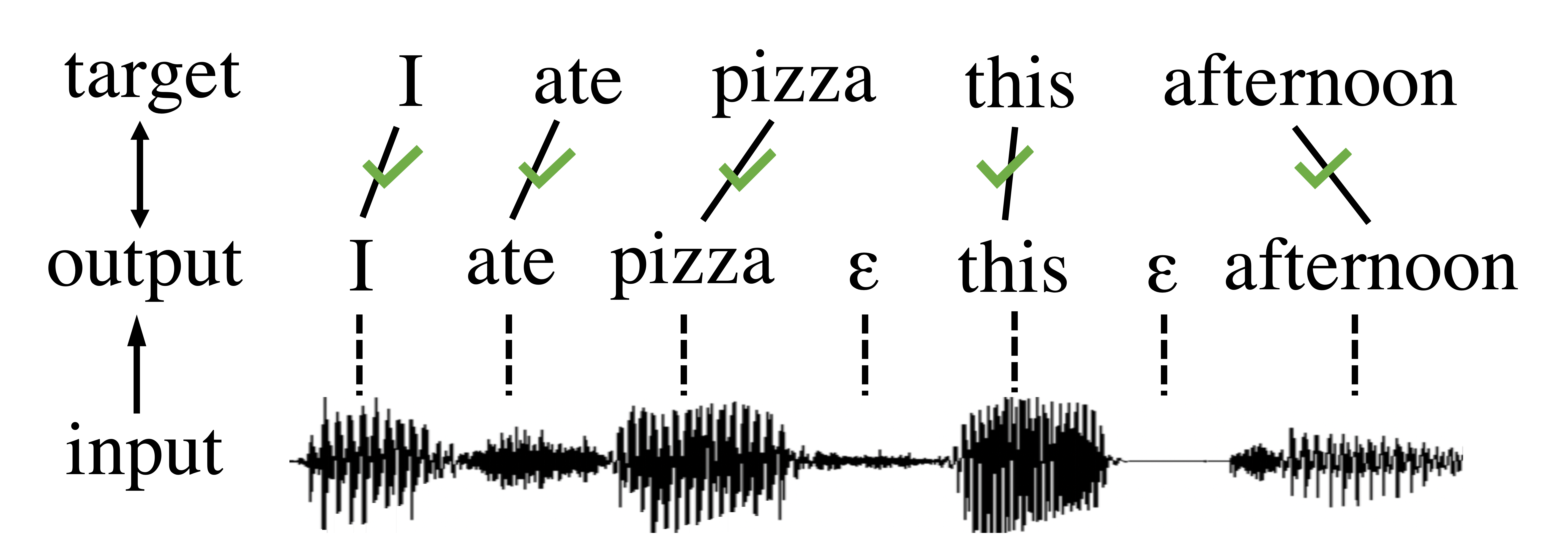
(a) CTC for ASR

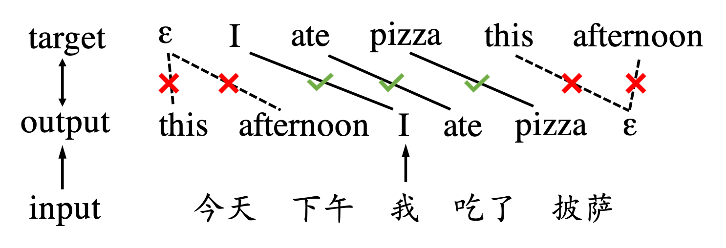
(b) CTC for NAT

Figure 1: Illustration of the monotonic alignment assumption of CTC: (a) CTC for ASR where there is a natural monotonic mapping between the speech input and ASR target, (b) CTC for NAT where there exists global word reordering that induces non-monotonic alignment. $\epsilon$ is the blank token that means ‘output nothing’.

In this paper, we propose to model non-monotonic latent alignments for non-autoregressive machine translation. We first extend the alignment space from monotonic alignments to non-monotonic alignments to allow for the global word reordering in machine translation. Without the monotonic structure, we have to optimize the best alignment found by the Hungarian algorithm [46, 28, 7, 9] since it becomes difficult to marginalize out all non-monotonic alignments with dynamic programming. This difficulty can be overcome by not requiring an exact match between alignments and the target sentence. In practice, it is not necessary to have the translation include exact words as contained in the target sentence, but it would be favorable to have a large overlap between them. Therefore, we further extend the alignment space by considering all alignments that overlap with the target sentence. Specifically, we are interested in the overlap of n-grams, which is the core of some evaluation metrics (e.g., BLEU). We accumulate n-grams from all alignments regardless of their positions and non-monotonically match them to target n-grams. The latent alignment model is trained to maximize the F1 score of n-gram matching, which reflects the translation quality to a certain extent [32].

We conduct experiments on major WMT benchmarks for NAT (WMT14 En$\leftrightarrow$De, WMT16 En$\leftrightarrow$Ro), which shows that our method substantially improves the translation performance and achieves comparable performance to autoregressive Transformer with only one-iteration parallel decoding.

2 Background

2.1 Non-Autoregressive Machine Translation

[17] proposes non-autoregressive neural machine translation, which achieves significant decoding speedup by generating target words simultaneously. NAT breaks the dependency among target tokens and factorizes the joint probability of target words in the following form:

$$p(y|x,\theta)=\prod_{t=1}^{T}p_{t}(y_{t}|x,\theta),$$ (1)

where $x$ is the source sentence belonging to the input space $\mathcal{X},y=\{y_{1},...,y_{T}\}$ is the target sentence belonging to the output space $\mathcal{Y}$, and $p_{t}(y_{t}|x,\theta)$ indicates the translation probability in position $t$.

The vanilla-NAT has a length predictor that takes encoder states as input to predict the target length. During the training, the target length is set to the golden length, and the vanilla-NAT is trained with the cross-entropy loss, which explicitly aligns model outputs to target words:

$$\mathcal{L}_{CE}(\theta)=-\sum_{t=1}^{T}\log(p_{t}(y_{t}|x,\theta)).$$ (2)

2.2 NAT with Latent Alignments

The vanilla-NAT suffers from two major limitations. The first limitation is the explicit alignment required by the cross-entropy loss, which cannot be guaranteed due to the multi-modality problem and therefore leads to the inaccuracy of the loss. The second limitation is the requirement of target length prediction. The predicted length may not be optimal and cannot be changed dynamically, so it is often required to use multiple length candidates and re-score them to produce the final translation.

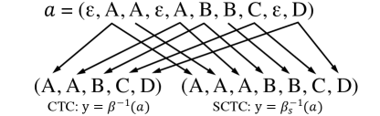
Figure 2: An example of target sentences obtained from collapsing functions of CTC and SCTC. The collapsing function of SCTC is $\beta_{s}^{-1}$, which only removeS blanks in the alignment $a$, where the collapsing function of CTC removes repetitions first and then removes blanks.

The two limitations can be addressed by using CTC-based latent alignment models [15, 29, 36], which extend the output space $\mathcal{Y}$ with a blank token $\epsilon$ that means ‘output nothing’. We define the extended output space as $\mathcal{Y}^{*}$. Following prior works [14, 36], we refer to the elements $a\in\mathcal{Y}^{*}$ as alignments, since the location of the blank tokens determines an alignment between the extended output and target sentence. Assume the generated alignments have length $T_{a}$, we define a function $\beta(y)$ which returns a subset of $\mathcal{Y}^{*}$ including all possible alignments of length $T_{a}$ for $y$, where $\beta^{-1}:\mathcal{Y}^{*}\mapsto\mathcal{Y}$ is the collapsing function that first collapses all consecutive repeated words in $a$ and then removes all blank tokens to obtain the target sentence. As illustrated in Figure 2, the alignment $a=(\epsilon,A,A,\epsilon,A,B,B,C,\epsilon,D)$ is collapsed to the target sentence $y=(A,A,B,C,D)$ with a monotonic mapping from target positions to alignment positions. During the training, latent alignment models marginalize all alignments with the CTC loss [15]:

$$\log p(y|x,\theta)=\log\sum_{a\in\beta(y)}p(a|x,\theta),$$ (3)

where the alignment probability $p(a|x,\theta)$ is modeled by a non-autoregressive Transformer:

$$p(a|x,\theta)=\prod_{t=1}^{T_{a}}p_{t}(a_{t}|x,\theta).$$ (4)

NAT models with latent alignments achieve superior performance by overcoming the two major limitations of NAT [29, 36, 16, 25, 33, 49]. The weakness in handling non-monotonic latent alignments is noticed in previous work [36, 16] but remains unsolved.

3 Approach

In this section, we explore non-monotonic latent alignments for NAT. We introduce a simplified CTC loss in section 3.1, which has a simpler structure that helps further analysis and derivation under the regular CTC loss. We explore non-monotonic alignments under the simplified CTC loss in section 3.2, and utilize the results to derive non-monotonic alignments under the regular CTC loss in section 3.3. Finally, we introduce the training strategy to combine monotonic and non-monotonic latent alignments in section 3.4.

3.1 Simplified Connectionist Temporal Classification

In CTC, the collapsing function $\beta^{-1}$ maps an alignment to a target sentence in two steps: (1) collapses all consecutive repeated words, (2) removes all blank tokens. The two operations make the alignment space $\beta(y)$ complex. Therefore, we first introduce the simplified connectionist temporal classification loss (SCTC), which has a simpler structure that helps the derivation of non-monotonic alignments, and the results on SCTC are helpful for further analysis under the regular CTC loss.

To simplify the alignment structure, we consider only using one operation in the collapsing function. One option is only collapsing all consecutive repeated words in the alignment. The concern is that it will limit the expressive power of the model. For example, the target sentence $y=(A,A,B,C,D)$ has probability 0 since it has repeated words that cannot be mapped from any alignment. Therefore, we favor another option that only removes all blank tokens. In this way, the expressive power stays the same and the alignment space becomes much simpler, where alignments of $y$ simply contain $T$ target words and $T_{a}-T$ blank tokens.

We denote this simplified loss as SCTC, and illustrate the difference between CTC and SCTC in Figure 2. The alignment space for the target sentence $y$ is defined as $\beta_{s}(y)$, and the collapsing function is defined as $\beta_{s}^{-1}$. We can still obtain the translation probability $p(y|x,\theta)$ with dynamic programming. We define the forward variable $\alpha_{t}(s)$ to be the total probability of $y_{1:s}$ considering all possible alignments $a_{1:t}$, which can be calculated recursively from $\alpha_{t-1}(s)$ and $\alpha_{t-1}(s-1)$:

$$\alpha_{t}(s)=\alpha_{t-1}(s-1)p_{t}(y_{s}|x,\theta)+\alpha_{t-1}(s)p_{t}(\epsilon|x,\theta).$$ (5)

Finally, the total translation probability $p(y|x,\theta)$ is given by the forward variable $\alpha_{T_{a}}(T)$, so we can train the model with the cross-entropy loss $\mathcal{L}_{sctc}(\theta)=-\log\alpha_{T_{a}}(T)$.

3.2 Non-Monotonic Alignments under SCTC

3.2.1 Bipartite Matching

In this section, we explore non-monotonic alignments under the SCTC loss, which are helpful for further analysis under the regular CTC loss. We first extend the alignment space from monotonic alignments $\beta_{s}(y)$ to non-monotonic alignments $\gamma_{s}(y)$ to allow for the global word reordering in machine translation, where $\gamma_{s}(y)$ is defined as:

$$\gamma_{s}(y)=\mathop{\cup}_{y^{\prime}\in P(y)}\beta_{s}(y^{\prime}).$$ (6)

In the above definition, $P(y)$ represents all permutations of $y$. For example, $P((A,B))=\{(A,B),(B,A)\}$. By enumerating $P(y)$, we consider all possible word reorderings of the target sentence. Ideally, we want to traverse all alignments in $\gamma_{s}(y)$ to calculate the log-likelihood loss:

$$\mathcal{L}_{sum}(\theta)=-\log\sum_{a\in\gamma_{s}(y)}p(a|x,\theta).$$ (7)

However, without the monotonic structure, it becomes difficult to marginalize out all latent alignments with dynamic programming. Alternatively, we can minimize the loss of the best alignment, which is an upper bound of Equation 7:

$$\mathcal{L}_{max}(\theta)=-\log\max_{a\in\gamma_{s}(y)}p(a|x,\theta).$$ (8)

Following prior work [46, 7, 9], we formulize finding the best alignment as a maximum bipartite matching problem and solve it with the Hungarian algorithm [28]. Specifically, we observe that the alignment space $\gamma_{s}(y)$ is simply permutations of $T$ target words and $T_{a}-T$ blank tokens. Therefore, finding the best alignment is equivalent to finding the best bipartite matching between the $T_{a}$ model predictions and the $T$ target words plus $T_{a}-T$ blank tokens, where the two sets of nodes are connected by edges with the prediction log-probability as weights.

3.2.2 N-Gram Matching

Without the monotonic structure desired for dynamic programming, calculating Equation 7 becomes difficult. This difficulty is also caused by the strict requirement of exact match for alignments, which makes it intractable to simplify the summation of probabilities. In practice, it is not necessary to force the exact match between alignments and the target sentence since a large overlap is also favorable. Therefore, we further extend the alignment space by considering all alignments that overlap with the target sentence. Specifically, we are interested in the overlap of n-grams, which is the core of some evaluation metrics (e.g., BLEU).

We propose a non-monotonic and non-exclusive n-gram matching objective based on SCTC to encourage the overlap of n-grams. Following the underlying idea of probabilistic matching [39], we introduce the probabilistic variant of the n-gram count to make the objective differentiable.

Specifically, we use $C_{g}(y)$ to denote the occurrence count of n-gram $g=(g_{1},...,g_{n})$ in the target sentence $y$, and use $C_{g}^{s}(\theta)$ to denote the probabilistic count of n-gram $g$ for the model with input $x$ and parameter $\theta$, where the superscript $s$ indicates SCTC. For simplicity, we omit the source sentence $x$ in $C_{g}^{s}(\theta)$ and the following notations. The probabilistic n-gram count is obtained by accumulating n-grams from all possible target sentences:

$$C_{g}^{s}(\theta)= \sum_{y\in\mathcal{Y}}p(y|x,\theta)C_{g}(y)=\sum_{a\in\mathcal{Y^{*}}}p(a|x,\theta)C_{g}(\beta_{s}^{-1}(a)).$$ (9)

The calculation of $C_{g}^{s}(\theta)$ is the core of this method and will be described in detail later. We use $M_{g}^{s}(\theta)$ to denote the match count of n-gram g between the latent alignment model and the target sentence $y$ (we omit $y$ in $M_{g}^{s}(\theta)$ for simplicity), which is defined as follows:

$$M_{g}^{s}(\theta)=\min(C_{g}(y),C_{g}^{s}(\theta)).$$ (10)

Our objective is to maximize the n-gram overlap between the target sentence and model output, so we can train the model to maximize the precision or recall of n-gram matching:

$$P_{n}^{s}(\theta)=\frac{\sum_{g\in G_{n}}M_{g}^{s}(\theta)}{\sum_{g\in G_{n}}C_{g}^{s}(\theta)},R_{n}^{s}(\theta)=\frac{\sum_{g\in G_{n}}M_{g}^{s}(\theta)}{\sum_{g\in G_{n}}C_{g}(y)},$$ (11)

where we use $G_{n}$ to denote the set of all n-grams. However, since latent alignment models have the ability to control the translation length, both precision and recall cannot accurately reflect the translation quality. The precision will encourage short translations to reduce the denominator, while the recall prefers long translations. Therefore, we consider both of them and maximize the F1 score:

$$\mathcal{L}_{n}^{s}(\theta)=-\text{F1}_{n}^{s}(\theta)=-\frac{2\cdot\sum_{g\in G_{n}}M_{g}^{s}(\theta)}{\sum_{g\in G_{n}}(C_{g}(y)+C_{g}^{s}(\theta))},$$ (12)

where we use $G_{n}$ to denote the set of all n-grams. In the numerator of Equation 12, $M_{g}^{s}(\theta)$ is non-zero only if $C_{g}(y)$ is non-zero, so we only need to calculate probabilistic n-gram counts $C_{g}^{s}(\theta)$ for n-grams $g$ in the target sentence. In the denominator, $\sum_{g\in G_{n}}C_{g}(y)$ equals to the constant $T-n+1$. Therefore, there are only two tasks left: calculating $C_{g}^{s}(\theta)$ and the summation $\sum_{g\in G_{n}}C_{g}^{s}(\theta)$.

For the first task of calculating $C_{g}^{s}(\theta)$, we first consider the simple case $n=1$. The main difference between 1-gram matching and bipartite matching is that 1-gram matching is non-exclusive, which allows us to marginalize out all alignments using the property of non-autoregressive generation. Due to the space limit, we refer readers to Appendix.A for the derivation and directly give the probabilistic 1-gram count as follows:

$$C_{g}^{s}(\theta)=\mathop{\sum}_{t=1}^{T_{a}}p_{t}(g_{1}|x,\theta),g\in G_{1},$$ (13)

where $G_{1}$ denotes the set of all 1-grams $g=(g_{1})$. Both 1-gram matching and bipartite matching are completely non-monotonic, which aim at generating correct target words regardless of the word order. When the target sentence is “I ate pizza this afternoon”, they will think that “pizza ate I this afternoon” is also a good translation. We consider 2-gram matching to overcome this limitation, which is also non-monotonic but takes target dependency into consideration. We first introduce a transition matrix $A$ of size $T_{a}\times T_{a}$, where $A_{i,j}$ is the probability that all positions between $i$ and $j$ are blank tokens:

$$A_{i,j}=\begin{cases}0&j<i+1\\ 1&j=i+1\\ \prod_{t=i+1}^{j-1}p_{t}(\epsilon|x,\theta)&j>i+1\end{cases}.$$ (14)

Then we give the probabilistic 2-gram count for $g=(g_{1},g_{2})$ (see Appendix.A for derivation):

$$C_{g}^{s}(\theta)=\mathop{\sum}_{i=1}^{T_{a}}\sum_{j=1}^{T_{a}}p_{i}(g_{1}|x,\theta)A_{i,j}p_{j}(g_{2}|x,\theta),g\in G_{2}.$$ (15)

For a larger $n$, the probabilistic n-gram count is:

$$C_{g}^{s}(\theta)=\sum_{i_{1}=1}^{T_{a}} \sum_{i_{2}=1}^{T_{a}}...\sum_{i_{n}=1}^{T_{a}}p_{i_{1}}(g_{1}|x,\theta)\times\prod_{k=2}^{n}A_{i_{k-1},i_{k}}p_{i_{k}}(g_{k}|x,\theta),\ g\in G_{n}.$$ (16)

Equation 15 can be efficiently calculated in matrix form with $\mathcal{O}(T_{a}^{2})$ time complexity. For Equation 16, we need $\mathcal{O}(nT_{a}^{n})$ operations to calculate it by brute force, which is impractical when $n$ is large. We refer readers to Appendix.B for the $\mathcal{O}(nT_{a}^{2})$ algorithm, which is similar to calculating the n-step transition probability of a Markov chain.

For the second task of efficiently calculating the summation of probabilistic n-gram counts $\sum_{g\in G_{n}}C_{g}^{s}(\theta)$, we also consider the simple case $n=1$ first, where the summation can be calculated by directly summing all probabilities:

$$\sum_{g}C_{g}^{s}(\theta)=\mathop{\sum}_{t=1}^{T_{a}}\sum_{g}p_{t}(g_{1}|x,\theta),g\in G_{1}.$$ (17)

For $n>1$, the search space is too big for the direct summation. Fortunately, the definition of $C_{g}^{s}(\theta)$ in Equation 9 allows us to safely extend the result of $n=1$ to a larger $n$ since n-grams count in a sentence is always $n-1$ less than 1-grams count.

$$\sum_{g\in G_{n}}C_{g}^{s}(\theta)=\mathop{\sum}_{g\in G_{1}}C_{g}^{s}(\theta)-n+1.$$ (18)

In summary, with the above results (Equation 13-18), we are able to efficiently calculate the loss defined in Equation 12 to maximize the F1 score of non-monotonic n-gram matching, which reflects the translation quality to a certain extent.

3.3 Non-Monotonic Alignments under CTC

In this section, we explore non-monotonic latent alignments under the regular CTC loss. Under SCTC, we can use both the bipartite matching and n-gram matching to train the latent alignment model. However, bipartite matching is infeasible under the regular CTC loss. Recall that the search space $\gamma_{s}(y)$ is simply permutations of target words and $T_{a}-T$ blank tokens, which allows us to find the best alignment with the Hungarian algorithm. However, as consecutive repeated words will be collapsed in the regular CTC loss, alignments in $\gamma(y)$ may contain different words, so the best alignment cannot be found by the Hungarian algorithm.

Fortunately, for n-gram matching, we can utilize previous results of SCTC to help the analysis and derivation under the regular CTC loss. As the output of the collapsing function $\beta_{s}^{-1}(a)$ simply contains more repeated words than $\beta^{-1}(a)$, we can first identify how much influence these repeated words have, and then remove this influence from the results of SCTC. We first formally define the probabilistic n-gram count under the regular CTC:

$$C_{g}(\theta)=\sum_{a\in\mathcal{Y}^{*}}p(a|x,\theta)C_{g}(\beta^{-1}(a)).$$ (19)

We define $R_{g}(\theta)$ to be the gap bewteen $C_{g}(\theta)$ and $C_{g}^{s}(\theta)$ when $n=1$, which represents the number of repeated words $g_{1}$ removed by the collapsing function. $R_{g}(\theta)$ can be efficiently calculated as follows (see Appendix.C for derivation):

$$R_{g}(\theta)=C_{g}^{s}(\theta)-C_{g}(\theta)=\sum_{t=1}^{T_{a}-1}p_{t}(g_{1}|x,\theta)p_{t+1}(g_{1}|x,\theta),g\in G_{1}.$$ (20)

The above equation enables us to efficiently calculate $C_{g}(\theta)$ and $\sum_{g}C_{g}(\theta)$ when $g\in G_{1}$. For 2-grams $g=(g_{1},g_{2})$, we divide it into two cases $g_{1}=g_{2}$ and $g_{1}\neq g_{2}$. The collapsing of consecutive repeated words will only remove 2-grams of the first case, where each removed word corresponds to a removed 2-gram. Taking Figure 2 as an example, the output of SCTC $\beta_{s}^{-1}(a)$ have two more 2-grams $\{(A,A),(B,B)\}$ of the $g_{1}=g_{2}$ case than the output of CTC $\beta^{-1}(a)$, and they contain exactly the same 2-grams of the $g_{1}\neq g_{2}$ case. Therefore, we can directly reuse previous results of SCTC and the number of repeated words $R_{g}(\theta)$ to calculate the probabilistic 2-gram count:

$$C_{g}(\theta)=\begin{cases}C_{g}^{s}(\theta)-R_{g}(\theta),&g_{1}=g_{2}\\ C_{g}^{s}(\theta),&g_{1}\neq g_{2}\end{cases},g\in G_{2}.$$ (21)

Unfortunately, for $n>2$, there is no such a clear relationship between $C_{g}(\theta)$ and $C_{g}^{s}(\theta)$, where the CTC output can contain n-grams (for example, $(A,B,C)$ in Figure 2) that the SCTC output does not have. If we directly formulize $C_{g}(\theta)$ like in Equation 16, it will be more complex and the $\mathcal{O}(nT_{a}^{2})$ algorithm is no longer applicable. Therefore, we do not use n-gram matching with $n>2$ under the regular CTC loss. Finally, we define the match count $M_{g}(\theta)$ similarly as in Equation 10 and train the CTC-based latent alignment model to maximize the F1 score:

$$\mathcal{L}_{n}(\theta)=-\frac{2\cdot\sum_{g\in G_{n}}M_{g}(\theta)}{\sum_{g\in G_{n}(C_{g}(y)+C_{g}(\theta))}}.$$ (22)

3.4 Training

In the above, we propose non-monotonic training objectives for the latent alignment model. They need to be combined with monotonic training objectives, otherwise, they may generate translations like “pizza ate I this afternoon”. Therefore, we first pretrain the latent alignment model with monotonic training objectives like SCTC or CTC. The model pretrained by SCTC can be finetuned with the bipartite matching objective (Equation 8) or the n-gram matching objective (Equation 12). The model pretrained by CTC can be finetuned with the n-gram matching objective (Equation 22), and the choices of $n$ are limited to $\{1,2\}$.

4 Experiments

4.1 Experimental Setup

Datasets We evaluate our methods on the most widely used public benchmarks in previous NAT studies: WMT14 English$\leftrightarrow$German (En$\leftrightarrow$De, 4.5M sentence pairs) [5] and WMT16 English$\leftrightarrow$Romanian (En$\leftrightarrow$Ro, 0.6M sentence pairs) [6]. For WMT14 En$\leftrightarrow$De, the validation set is newstest2013 and the test set is newstest2014. For WMT16 En$\leftrightarrow$Ro, the validation set is newsdev-2016 and the test set is newstest-2016. Following prior works, we use tokenized BLEU [32] to evaluate the translation quality. Considering that BLEU might be biased as our method optimizes the n-gram overlap, we also report METEOR [2], which is not directly based on n-gram overlap. We learn a joint BPE model [37] with 32K operations to process the data and share the vocabulary for source and target languages.

Knowledge Distillation Following prior works [17], we apply sequence-level knowledge distillation [26] to reduce the complexity of training data. We use Transformer-base setting for the teacher model and train NAT on the distilled data.

Implementation Details We adopt Transformer-base [47] as our autoregressive baseline as well as the teacher model. We uniformly copy encoder outputs to construct decoder inputs. For CTC-based NAT models, the length for decoder inputs is 3$\times$ as long as the source length. On WMT14 En$\leftrightarrow$De, we use a dropout rate of 0.2 to train NAT models and use a dropout rate of 0.1 for finetuning. On WMT16 En$\leftrightarrow$Ro, the dropout rate is 0.3 for both the pretraining and finetuning. We use the batch size 64K and train NAT models for 300K steps on WMT14 En$\leftrightarrow$De and 150K steps on WMT16 En$\leftrightarrow$Ro. During the finetuning, we train NAT models for 6K steps with the batch size 256K. All models are optimized with Adam [27] with $\beta=(0.9,0.98)$ and $\epsilon=10^{-8}$. The learning rate warms up to $5\cdot 10^{-4}$ within 10K steps in the pretraining and warms up to $e\cdot 10^{-4}$ within 500 steps in the finetuning. We use the GeForce RTX 3090 GPU to train models and measure the translation latency. We implement our models based on the open-source framework of fairseq [MIT License, 31].

Table 1: Performance comparison between baselines and our methods on WMT14 En-De test set.

	Model	BLEU	METEOR	Speed
Base	Transformer	27.54	54.38	1.0$\times$
	Vanilla-NAT	19.32	45.79	15.5$\times$
SCTC	SCTC	25.26	52.06	14.7$\times$
	+bipartite	26.13	53.17
	+1-gram	26.22	53.20
	+2-gram	26.79	53.54
	+3-gram	26.66	53.48
	+4-gram	26.62	53.43
CTC	CTC	26.34	53.15	14.7$\times$
	+1-gram	27.16	53.95
	+2-gram	27.57	54.50

Table 2: Performance comparison between our models and existing methods. The speedup is measured on WMT14 En-De test set with batch size 1. AT means autoregressive. Iter. denotes the number of iterations at inference time. ‘–’ indicates that the result is not reported. ‘12-1’ means the Transformer with 12 encoder layers and 1 decoder layer [24].

Models		Iter.	Speed	WMT14		WMT16
	EN-DE			DE-EN	EN-RO	RO-EN
AT	Transformer (teacher)	N	1.0$\times$	27.54	31.57	34.26	33.87
	Transformer (12-1)	N	2.6$\times$	26.09	30.30	32.76	32.39
	+ KD	N	2.7$\times$	27.61	31.48	33.43	33.50
	NAT-FT [17]	1	15.6$\times$	17.69	21.47	27.29	29.06
	NAT-REG [48]	1	27.6$\times$	20.65	24.77	–	–
	AXE [13]	1	–	23.53	27.90	30.75	31.54
	GLAT [33]	1	15.3$\times$	25.21	29.84	31.19	32.04
Non-CTC	Seq-NAT [42]	1	15.6$\times$	25.54	29.91	31.69	31.78
NAT	AligNART [45]	1	13.4$\times$	26.40	30.40	32.50	33.10
	CMLM [12]	10	–	27.03	30.53	33.08	33.31
	LevT [18]	2.05	4.0$\times$	27.27	–	–	33.26
	JM-NAT [19]	10	–	27.69	32.24	33.52	33.72
	RewriteNAT [11]	2.70	–	27.83	31.52	33.63	34.09
	CMLMC [22]	10	–	28.37	31.41	34.57	34.13
	CTC [29]	1	–	16.56	18.64	19.54	24.67
	Imputer [36]	1	–	25.80	28.40	32.30	31.70
	GLAT+CTC [33]	1	14.6$\times$	26.39	29.54	32.79	33.84
CTC-based	REDER [49]	1	15.5$\times$	26.70	30.68	33.10	33.23
NAT	+ beam&reranking	1	5.5$\times$	27.36	31.10	33.60	34.03
	DSLP [21]	1	14.8$\times$	27.02	31.61	34.17	34.60
	Fully-NAT [16]	1	16.8$\times$	27.20	31.39	33.71	34.16
	Imputer [36]	8	–	28.20	31.80	34.40	34.10
	Bag-of-ngrams [41]	1	15.5$\times$	25.28	29.66	31.37	31.51
Our	+ rescore 5 candidates	1	9.5$\times$	25.95	30.43	32.78	32.92
Implementation	OAXE [9]	1	15.3$\times$	24.70	29.30	31.06	31.37
	+ rescore 5 candidates	1	14.0 $\times$	25.78	30.29	32.45	32.63
Our work	CTC w/o finetune	1	14.7$\times$	26.34	29.58	33.45	33.32
	CTC w/ NMLA	1	14.7$\times$	27.57	31.28	33.86	33.94
	+ beam&lm	1	5.0$\times$	28.35	32.27	34.72	34.95
	DDRS w/o finetune	1	14.7$\times$	27.18	30.91	34.42	34.31
	DDRS w/ NMLA	1	14.7$\times$	28.02	31.80	34.73	34.76
	+ beam&lm	1	5.0$\times$	28.63	32.65	35.51	35.85

Decoding For autoregressive models, we use beam search with beam size 5 for the decoding. For Vanilla-NAT, we use argmax decoding to generate the translation. For CTC-based models, we can also use argmax decoding to generate the alignment and then collapse it to obtain the translation. Besides, following [29, 16], we can use beam search decoding combined with a 4-gram language model [20] to find the translation that maximizes:

$$\log p(y|x,\theta)+\alpha\log p_{LM}(y)+\beta\log(|y|),$$ (23)

where $\alpha$ and $\beta$ are hyperparameters for the language model score and length bonus. We use a fixed beam size 20 with grid-search $\alpha$, $\beta$. The beam search does not contain any neural network computations and can be implemented efficiently in C++.

4.2 Main Results

We first compare the performance of different non-monotonic training objectives for latent alignment models. Baseline models include the Transformer, vanilla-NAT, SCTC, and CTC, and we finetune latent alignment models with bipartite matching and n-gram matching objectives. In Table 1, we report BLEU and METEOR scores along with the speedup on WMT14 En-De test set.

From Table 1, we have the following observations: (1) Non-monotonic training objectives can effectively improve the performance of latent alignment models, which improves SCTC by 1.53 BLEU and 1.48 METEOR and improves CTC by 1.23 BLEU and 1.35 METEOR, illustrating the importance of non-monotonic alignments. (2) Despite having the same expressive power, SCTC underperforms CTC in the task of non-autoregressive translation. We speculate that it is because of the difference in the distribution of the alignment space. Most target sentences do not contain repeated words, in which case the alignment space of SCTC $\beta_{s}^{-1}(y)$ is a subset of $\beta^{-1}(y)$, making the ability of SCTC relatively weak. (3) SCTC achieves the best performance with 2-gram finetuning, and then the performance decreases with the increase of n due to the sparsity of higher rank n-grams. It suggests that we do not need a large n and relieves the concern on CTC that we cannot calculate n-gram matching for $n>2$. (4) The correlation between the reported BLEU and METEOR scores is very strong, suggesting that BLEU is not biased when evaluating our methods. Therefore, we can safely use BLEU to evaluate the translation quality in the following experiments.

We call the 2-gram matching objective NMLA since it represents our best non-monotonic training method for latent alignment models. Besides CTC, we also apply NMLA finetuning on a stronger baseline DDRS [43], which trains the CTC model with multiple references. To extend our method to multiple references, we calculate the n-gram counts for each reference and use their average as the target n-gram count. We compare their performance with existing approaches in Table 2. Notably, CTC with NMLA achieves comparable performance to autoregressive Transformer on all benchmarks, demonstrating the effectiveness of our method. On the strong baseline DDRS, NMLA finetuning also brings remarkable improvements and outperforms autoregressive baselines. With the help of beam search and 4-gram language model, NMLA even outperforms other iterative NAT models and the autoregressive Transformer with only one-iteration parallel decoding. Compared to our implementations of prior works that explore non-monotonic matching for NAT [41, 9], we can see that they underperform the CTC baseline even when rescoring 5 candidates, and their speedup after rescoring also lays behind CTC. It demonstrates the importance of exploring non-monotonic matching on latent alignment models, which is more desirable for its flexibility of generating predictions with variable lengths.

As NMLA finetuning brings remarkable improvements over the strong baseline DDRS, we further conduct experiments to verify whether the NMLA is orthogonal to other methods. In Table 4.2, we reimplement GLAT+CTC (Fully-NAT) [16, 33] based on their open-source code and finetune it with the NMLA objective. Our implementation replaces the SoftCopy mechanism with UniformCopy, which surprisingly improves 0.7 BLEU and achieves 27.07 BLEU on WMT14 En-De test set. Finetuning with NMLA can further improve its performance to 27.75 BLEU, demonstrating the extensibility of NMLA. In Table 4.2, we apply NMLA on the big version of DDRS to explore its capability on large models. The results show that the performance of DDRS-big can be greatly boosted by NMLA finetuning. Combined with beam search, it achieves 30.06 BLEU on WMT14 En-De, which narrows the performance gap between non-autoregressive and autoregressive models to a new level.

tableBLEU scores of GLAT+CTC and NMLA finetuning on WMT14 En-De test set. Model BLEU Speed GLAT+CTC w/o finetune 27.07 14.7$\times$ GLAT+CTC w/ NMLA 27.75 14.7$\times$     + beam&lm 28.46 5.0$\times$

tableBLEU scores of DDRS-big and NMLA finetuning on WMT14 En-De test set. Model BLEU Speed DDRS-big w/o finetune 28.24 14.1$\times$ DDRS-big w/ NMLA 29.11 14.1$\times$     + beam&lm 30.06 4.8$\times$

4.3 Training Cost

In this section, we will analyze the training cost and show that our method is cost-effective. The additional training cost of our method only comes from the NMLA finetuning. In Table 3, we compare the training cost of CTC and NMLA on WMT14 En-De. We measure the training speed by Words Per Second (WPS) and find that the training speed of NMLA is slower than CTC, which can be attributed to the large calculation cost of the NMLA objective. However, since we only finetune the model for 6K steps, the overall cost of the NMLA finetuning is much smaller than the CTC pretraining. On the whole, the training cost of CTC with NMLA is less than $1.2\times$ compared to the CTC baseline.

Table 3: The comparison of CTC pretraining and NMLA finetuning. ’WPS’ means words per second. ’Step’ means the number of training steps. ’Batch’ means batch size. ’Time’ means the training time measured on 8 GeForce RTX 3090 GPUs.

	WPS	Step	Batch	Time
CTC pretraining	141K	300K	64K	26.4h
NMLA finetuning	60K	6K	256K	5.0h

5 Related Work

[17] first proposes non-autoregressive machine translation to accelerate the decoding process of NMT. The cross-entropy loss is applied to train the Vanilla-NAT, which requires the explicit alignment between the model output and target sentence. The explicit alignment cannot be guaranteed due to the multi-modality problem, and many efforts have been devoted to mitigating this issue.

One research direction is to enable explicit alignment by leaking part of the target-side information during the training. [17] uses fertilities as a latent variable to specify the number of output words corresponding to each input word. [23, 35, 4] apply vector quantization to train NAT with discrete latent variables, and [30, 44, 16] apply variational inference to train NAT with continuous latent variables. [34, 3, 45] also introduce latent variables that carry the reordering information. Besides using latent variables, [12] directly feeds the partially masked target sentence as the decoder input, and [33] applies a glancing sampling strategy to control the mask ratio.

Another research direction is to propose better training objectives for NAT. [48] introduces two auxiliary regularization terms to reduce errors of repeated translations and incomplete translations. [40] directly optimizes sequence-level objectives with reinforcement learning. [21] trains NAT with deep supervision and feeds additional layer-wise predictions. [43] creates a dataset with multiple references and dynamically selects an appropriate reference for the training. Prior to this work, [41, 13, 9] have explored ways to establish an alignment between the model output and target sentence, which can promote the training of NAT. Their limitation is that they are basically built on the framework of Vanilla-NAT, which requires a target length predictor and cannot dynamically adjust the output sequence length. CTC-based latent alignment models [29, 36, 16] are more desirable due to their superior performance and the flexibility of generating predictions with variable lengths. However, latent alignment models have a weakness in handling non-monotonic alignments, which is noticed in previous work [36, 16] and solved in this work.

6 Conclusion

Latent alignment models cannot handle non-monotonic alignments during the training, which is nonnegligible in machine translation. In this paper, we explore non-monotonic latent alignments for NAT and propose two matching objectives named bipartite matching and n-gram matching. Experiments show that our method achieves strong improvements on latent alignment models.

7 Acknowledgement

We thank the anonymous reviewers for their insightful comments. This work was supported by National Key R&D Program of China (NO.2018AAA0102502).

Checklist

1. For all authors…

   1. Do the main claims made in the abstract and introduction accurately reflect the paper’s contributions and scope? [Yes]

   2. Did you describe the limitations of your work? [Yes]

   3. Did you discuss any potential negative societal impacts of your work? [No]

   4. Have you read the ethics review guidelines and ensured that your paper conforms to them? [Yes]

2. If you are including theoretical results…

   1. Did you state the full set of assumptions of all theoretical results? [Yes]

   2. Did you include complete proofs of all theoretical results? [Yes]

3. If you ran experiments…

   1. Did you include the code, data, and instructions needed to reproduce the main experimental results (either in the supplemental material or as a URL)? [Yes]

   2. Did you specify all the training details (e.g., data splits, hyperparameters, how they were chosen)? [Yes]

   3. Did you report error bars (e.g., with respect to the random seed after running experiments multiple times)? [No]

   4. Did you include the total amount of compute and the type of resources used (e.g., type of GPUs, internal cluster, or cloud provider)? [Yes]

4. If you are using existing assets (e.g., code, data, models) or curating/releasing new assets…

   1. If your work uses existing assets, did you cite the creators? [Yes]

   2. Did you mention the license of the assets? [Yes]

   3. Did you include any new assets either in the supplemental material or as a URL? [Yes]

   4. Did you discuss whether and how consent was obtained from people whose data you’re using/curating? [Yes]

   5. Did you discuss whether the data you are using/curating contains personally identifiable information or offensive content? [No]

5. If you used crowdsourcing or conducted research with human subjects…

   1. Did you include the full text of instructions given to participants and screenshots, if applicable? [N/A]

   2. Did you describe any potential participant risks, with links to Institutional Review Board (IRB) approvals, if applicable? [N/A]

   3. Did you include the estimated hourly wage paid to participants and the total amount spent on participant compensation? [N/A]

Appendix A Proof of Equation 13, Equation 15, and Equation 16

Equation 13 and and Equation 15 are the special cases of Equation 16 when n is 1 or 2, so we directly provide the proof of Equation 16:

$$C_{g}^{s}(\theta)=\mathop{\sum}_{i_{1}=1}^{T_{a}}\sum_{i_{2}=1}^{T_{a}}\ldots\sum_{i_{n}=1}^{T_{a}}p_{i_{1}}(g_{1}|x,\theta)\times\mathop{\prod}_{k=2}^{n}A_{i_{k-1},i_{k}}p_{i_{k}}(g_{k}|x,\theta),g\in G_{n}.$$

We begin with the definition of $C_{g}^{s}(\theta)$, which accumulates the n-gram $g$ from all alignments:

$$C_{g}^{s}(\theta)=\mathop{\sum}_{a\in\mathcal{Y^{*}}}p(a|x,\theta)C_{g}(\beta_{s}^{-1}(a)),$$

where $C_{g}(\beta^{-1}_{s}(a))$ is the occurrence count of n-gram g in the collapsed sentence $\beta^{-1}_{s}(a)$. We use $i_{1:n}=\{i_{1},...,i_{n}\}$ to denote the possible position of $g=\{g_{1},...,g_{n}\}\in G_{n}$. There is an n-gram $g\in G_{n}$ in the position $i_{1:n}$ if and only if $a_{i_{k}}=g_{k}$ for all $k\in\{1,...,n\}$ and all other words between them are blank tokens. By traversing all possible positions, we can obtain the n-gram count as follows:

$$C_{g}(\beta_{s}^{-1}(a))=\mathop{\sum}_{i_{1}=1}^{T_{a}}\sum_{i_{2}=1}^{T_{a}}\ldots\sum_{i_{n}=1}^{T_{a}}1(a_{i_{1}}=g_{1})\times\mathop{\prod}_{k=2}^{n}1(i_{k-1}<i_{k},a_{i_{k}}=g_{k},a_{i_{k-1}+1:i_{k}-1}=\epsilon),g\in G_{n}.$$

where $1(\cdot)$ is the indicator function that takes value $1$ when the inside condition holds, otherwise it takes value $0$. Recall that $A_{ij}$ is the probability that all positions between $i$ and $j$ are blank tokens, which satisfies the following equation:

$$A_{i_{k-1},i_{k}}=p(i_{k-1}<i_{k},a_{i_{k-1}+1:i_{k}-1}=\epsilon|x,\theta).$$

Using the above equations, we can rewrite $C_{g}^{s}(\theta)$ as:

$$C_{g}^{s}(\theta) =\mathop{\sum}_{a}p(a|x,\theta)C_{g}(\beta_{s}^{-1}(a))$$

$$=\mathop{\sum}_{i_{1}=1}^{T_{a}}\sum_{i_{2}=1}^{T_{a}}\ldots\sum_{i_{n}=1}^{T_{a}}\sum_{a}p(a|x,\theta)1(a_{i_{1}}=g_{1})\times\mathop{\prod}_{k=2}^{n}1(i_{k-1}<i_{k},a_{i_{k}}=g_{k},a_{i_{k-1}+1:i_{k}-1}=\epsilon)$$

$$=\mathop{\sum}_{i_{1}=1}^{T_{a}}\sum_{i_{2}=1}^{T_{a}}\ldots\sum_{i_{n}=1}^{T_{a}}p(a_{i_{1}}=g_{1}|x,\theta)\times\mathop{\prod}_{k=2}^{n}p(a_{i_{k}}=g_{k}|x,\theta)p(i_{k-1}<i_{k},a_{i_{k-1}+1:i_{k}-1}=\epsilon)$$

$$=\mathop{\sum}_{i_{1}=1}^{T_{a}}\sum_{i_{2}=1}^{T_{a}}\ldots\sum_{i_{n}=1}^{T_{a}}p_{i_{1}}(g_{1}|x,\theta)\times\mathop{\prod}_{k=2}^{n}A_{i_{k-1},i_{k}}p_{i_{k}}(g_{k}|x,\theta),g\in G_{n}.\ \ \square$$

Appendix B The $\mathcal{O}(nT_{a}^{2})$ algorithm for Equation 16

Here we give the $\mathcal{O}(nT_{a}^{2})$ algorithm to calculate $C_{g}^{s}(\theta)$ according to Equation 16. Notice that Equation 16 has a similar form with the n-step transition probability of a Markov chain, so we can try a similar method as calculating the transition probability for a Markov chain. Specifically, we introduce a set of state vectors $s_{k}$ , where $k\in\{1,2,...,T_{a}\}$ and the dimension of each vector $s_{k}$ is $T_{a}$ . We define the state vectors as follows:

$$s_{k}(i_{k})=\begin{cases}p_{i_{k}}(g_{k}|x,\theta),&k=1\\ \sum_{i_{k-1}=1}^{T_{a}}s_{k-1}(i_{k-1})A_{i_{k-1},i_{k}}p_{i_{k}}(g_{k}|x,\theta),&k>1\end{cases}.$$

From the above equation, the time complexity to calculate $s_{k}$ given $s_{k-1}$ is $\mathcal{O}(T_{a}^{2})$ and can be efficiently calculated in matrix form. Therefore, the time complexity to sequentially calculate $s_{1:n}$ is $\mathcal{O}(nT_{a}^{2})$. Finally, we can easily obtain $C_{g}^{s}(\theta)$ by summing the last vector $s_{n}$:

$$C_{g}^{s}(\theta) =\mathop{\sum}_{i_{1}=1}^{T_{a}}\sum_{i_{2}=1}^{T_{a}}\ldots\sum_{i_{n}=1}^{T_{a}}p_{i_{1}}(g_{1}|x,\theta)\times\mathop{\prod}_{k=2}^{n}A_{i_{k-1},i_{k}}p_{i_{k}}(g_{k}|x,\theta)$$

$$=\mathop{\sum}_{i_{n}=1}^{T_{a}}\ldots\sum_{i_{2}=1}^{T_{a}}\sum_{i_{1}=1}^{T_{a}}s_{1}(i_{1})\mathop{\prod}_{k=2}^{n}A_{i_{k-1},i_{k}}p_{i_{k}}(g_{k}|x,\theta)$$

$$=\mathop{\sum}_{i_{n}=1}^{T_{a}}\ldots\sum_{i_{3}=1}^{T_{a}}\sum_{i_{2}=1}^{T_{a}}s_{2}(i_{2})\mathop{\prod}_{k=3}^{n}A_{i_{k-1},i_{k}}p_{i_{k}}(g_{k}|x,\theta)$$

$$=......$$

$$=\mathop{\sum}_{i_{n}=1}^{T_{a}}\sum_{i_{n-1}=1}^{T_{a}}s_{n-1}(i_{n-1})\times A_{i_{n-1},i_{n}}p_{i_{n}}(g_{n}|x,\theta)$$

$$=\mathop{\sum}_{i_{n}=1}^{T_{a}}s_{n}(i_{n}),g\in G_{n}.\ \ \ \square$$

Appendix C Proof of Equation LABEL:eq:rg

Here we provide the proof of Equation LABEL:eq:rg:

$$R_{g}(\theta)=C_{g}^{s}(\theta)-C_{g}(\theta)=\mathop{\sum}_{t=1}^{T_{a}-1}p_{t}(g_{1}|x,\theta)p_{t+1}(g_{1}|x,\theta),g\in G_{1},$$

which is equivalent to proving the following equation:

$$C_{g}(\theta)=p_{1}(g_{1}|x,\theta)+\sum_{t=2}^{T_{a}}p_{t}(g_{1}|x,\theta)(1-p_{t-1}(g_{1}|x,\theta)),g\in G_{1}.$$

We begin with the definition of $C_{g}(\theta)$, which accumulates the n-gram $g$ from all alignments:

$$C_{g}(\theta)=\mathop{\sum}_{a\in\mathcal{Y^{*}}}p(a|x,\theta)C_{g}(\beta^{-1}(a)).$$

$C_{g}(\beta^{-1}(a))$ is the occurrence count of n-gram $g$ in the collapsed sentence $\beta^{-1}(a)$. Besides blank tokens, repeated words will also be removed by $\beta^{-1}$. Therefore, we call a word in the alignment a valid word when it does not repeat the word before it. We can calculate the 1-gram count by collecting all valid words, which will not be removed by the collapsing function:

$$C_{g}(\beta^{-1}(a))=1(a_{1}=g_{1})+\mathop{\sum}_{t=2}^{T_{a}}1(a_{t}=g_{1},a_{t-1}\neq g_{1}),g\in G_{1}.$$

Using the above equation, we can rewrite $C_{g}(\theta)$ as:

$$C_{g}(\theta) =\mathop{\sum}_{a}p(a|x,\theta)C_{g}(\beta^{-1}(a))=p(a_{1}=g_{1}|x,\theta)+\sum_{t=2}^{T_{a}}p(a_{t}=g_{1},a_{t-1}\neq g_{1}|x,\theta)$$

$$=p_{1}(g_{1}|x,\theta)+\sum_{t=2}^{T_{a}}p_{t}(g_{1}|x,\theta)(1-p_{t-1}(g_{1}|x,\theta)),g\in G_{1}.\ \ \ \square$$

Appendix D Analysis

To better understand our method, we present a qualitative analysis to provide some insights into the improvements of NMLA. We analyze the generated outputs of the WMT14 En-De test set in the following experiments.

NMLA Handles Long Sequences Better We first investigate the performance of AT and NAT models for different sequence lengths. We split the test set into different buckets based on target sequence length and calculate BLEU for each bucket. We report the results in Table 4. The first observation is that the performance of Vanilla-NAT drops drastically as the sequence length increases. It is a well-known property of NAT and can be explained as the increased probability of observing misalignment between model output and target as the target sequence becomes longer. The misalignment in long sequences causes the inaccuracy of loss and therefore harms the translation quality. We have a similar observation when comparing CTC with NMLA. The performance of CTC is close to NMLA on short sequences, but the gap becomes larger as the sequence length increases. Our explanation is that the longer the sequence, the more likely the monotonic assumption fails due to the global word reordering, which causes the inaccuracy of loss and therefore harms the translation quality. NMLA models non-monotonic alignments and alleviates the inaccuracy of loss on long sequences, so it achieves strong improvements on long sequences and even outperforms AT by more than 2 BLEU, which suffers from the error accumulation on long sequences.

Table 4: The performance of AT and NAT models with respect to the target sequence length. ‘Vanilla’ means Vanilla-NAT. ‘N’ denotes the target sequence length. ‘AT’ means autoregressive Transformer.

Length	Vanilla	CTC	AT	NMLA
$1\leq N<20$	21.27	24.83	25.68	25.55
$20\leq N<40$	19.49	26.81	28.05	27.82
$40\leq N<60$	16.21	26.54	26.71	27.74
$60\leq N$	10.69	26.69	26.44	28.89
All	19.32	26.34	27.54	27.57

NMLA Improves Model Confidence NAT suffers from the multi-modality problem, which makes the model consider many possible translations at the same time and become less confident in generating outputs. We investigate whether our method alleviates the multi-modality problem by measuring how confident the model is during the decoding. We use the information entropy to measure the confidence, which is calculated as $H(X)=-\sum_{x\in\mathcal{X}}p(x)\log p(x)$, and lower entropy indicates higher confidence. We calculate the entropy in every position when decoding the WMT14 En-De test set and use the average entropy to represent the model confidence. We do not report the entropy of AT since it varies with the decoding algorithm. The average entropy scores of NAT models are reported in Table 5. We can see that the Vanilla-NAT has low prediction confidence, which is substantially improved by CTC. NMLA further reduces the average entropy to $0.061$, showing that the model confidence can be improved by modeling non-monotonic latent alignments.

Table 5: The average prediction entropy of NAT models. ‘Vanilla’ means Vanilla-NAT.

	Vanilla	CTC	NMLA
Entropy	2.098	0.260	0.061

NMLA Improves Generation Fluency Since NAT generates target words independently, generation fluency is a main weakness of NAT. The multi-modality problem makes NAT consider many possible translations at the same time and generate an inconsistent output, which further reduces the generation fluency. We investigate whether our method improves the generation fluency with an n-gram language model [20] trained on the target side of WMT14 En-De training data. We use the language model to calculate the perplexity scores of model outputs and report the results in Table 6. We can see that Vanilla-NAT and CTC have high perplexity which indicates low fluency. NMLA substantially reduces the perplexity score, which is only 42.6 higher than the gold reference. For AT, its perplexity score is even lower than the gold reference, which is consistent with prior works that autoregressive NMT generally improves fluency at the cost of adequacy [8, 10].

Table 6: The perplexity scores of AT and NAT models on WMT14 En-De test set.

	Vanilla	CTC	NMLA	AT	Gold
PPL	597.0	315.5	258.8	197.0	216.2

Appendix E Batch Speedup

For CTC-based models including NMLA, a common concern is that they require a larger number of calculations than the autoregressive model due to the longer decoder length. Though there is a significant speedup when decoding sentence by sentence, this advantage may disappear when we use a larger decoding batch. In response to this concern, we measure the decoding speedup on WMT14 En-De test set under different batch sizes and report both BLEU and speedup in Figure 3. Under the memory limit, the maximum batch size is $400$. From Figure 3, NMLA still maintains $2.4\times$ speedup under the maximum batch size while achieving comparable performance to the autoregressive model. For NMLA+beam&lm, it simultaneously achieves superior translation quality and speed to the autoregressive model, which addresses the concern on batch speedup for CTC-based models.

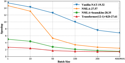
Figure 3: BLEU and speedup of NAT and AT models measured under different batch sizes on WMT14 En-De test set.

Appendix F Combination of N-grams

In Table 1, we only finetune the baseline with different n-gram matching objectives respectively. Here we combine different n-gram matching objectives to see whether the combination can improve the model performance. First, we linearly combine 1-gram and 2-gram matching with a hyperparameter $\alpha$:

$$\mathcal{L}(\theta)=\alpha\cdot\mathcal{L}_{1}({\theta})+(1-\alpha)\cdot\mathcal{L}_{2}({\theta}),\ \ \ \mathcal{L}^{s}(\theta)=\alpha\cdot\mathcal{L}_{1}^{s}({\theta})+(1-\alpha)\cdot\mathcal{L}_{2}^{s}({\theta}).$$

We train CTC and SCTC baselines with different $\alpha$ and report the results in Table 7, which shows that the combination of 1-gram and 2-gram underperforms simply using 2-gram matching.

Table 7: BLEU scores of SCTC and CTC under different $\alpha$ on WMT14 En-De validation set.

$\alpha$	0	0.25	0.5	0.75	1
SCTC	25.09	24.98	24.85	24.70	24.54
CTC	25.90	25.74	25.66	25.51	25.42

As $n>2$ is allowed in SCTC, we further try to combine higher rank n-grams. We consider $n\in\{1,2,3,4\}$ and combine them with arithmetic average and geometric average respectively. The BLEU scores of arithmetic average and geometric average are respectively $24.94$ BLEU and $24.88$ BLEU on WMT14 En-De validation set, which also underperforms simply using 2-gram matching. Therefore, we conclude that simply combining different n-gram matching objectives cannot improve the model performance.

References

- Bahdanau et al. [2015] D. Bahdanau, K. Cho, and Y. Bengio. Neural machine translation by jointly learning to align and translate. In Y. Bengio and Y. LeCun, editors, 3rd International Conference on Learning Representations, ICLR 2015, San Diego, CA, USA, May 7-9, 2015, Conference Track Proceedings, 2015. URL http://arxiv.org/abs/1409.0473.
- Banerjee and Lavie [2005] S. Banerjee and A. Lavie. METEOR: An automatic metric for MT evaluation with improved correlation with human judgments. In Proceedings of the ACL Workshop on Intrinsic and Extrinsic Evaluation Measures for Machine Translation and/or Summarization, pages 65–72, Ann Arbor, Michigan, June 2005. Association for Computational Linguistics. URL https://aclanthology.org/W05-0909.
- Bao et al. [2019] Y. Bao, H. Zhou, J. Feng, M. Wang, S. Huang, J. Chen, and L. Lei. Non-autoregressive transformer by position learning. arXiv preprint arXiv:1911.10677, 2019.
- Bao et al. [2021] Y. Bao, S. Huang, T. Xiao, D. Wang, X. Dai, and J. Chen. Non-autoregressive translation by learning target categorical codes. In Proceedings of the 2021 Conference of the North American Chapter of the Association for Computational Linguistics: Human Language Technologies, pages 5749–5759, Online, June 2021. Association for Computational Linguistics. doi: 10.18653/v1/2021.naacl-main.458. URL https://aclanthology.org/2021.naacl-main.458.
- Bojar et al. [2014] O. Bojar, C. Buck, C. Federmann, B. Haddow, P. Koehn, J. Leveling, C. Monz, P. Pecina, M. Post, H. Saint-Amand, R. Soricut, L. Specia, and A. Tamchyna. Findings of the 2014 workshop on statistical machine translation. In Proceedings of the Ninth Workshop on Statistical Machine Translation, pages 12–58, Baltimore, Maryland, USA, June 2014. Association for Computational Linguistics. URL http://www.aclweb.org/anthology/W/W14/W14-3302.
- Bojar et al. [2016] O. Bojar, R. Chatterjee, C. Federmann, Y. Graham, B. Haddow, M. Huck, A. Jimeno Yepes, P. Koehn, V. Logacheva, C. Monz, M. Negri, A. Neveol, M. Neves, M. Popel, M. Post, R. Rubino, C. Scarton, L. Specia, M. Turchi, K. Verspoor, and M. Zampieri. Findings of the 2016 conference on machine translation. In Proceedings of the First Conference on Machine Translation, pages 131–198, Berlin, Germany, August 2016. Association for Computational Linguistics. URL http://www.aclweb.org/anthology/W/W16/W16-2301.
- Carion et al. [2020] N. Carion, F. Massa, G. Synnaeve, N. Usunier, A. Kirillov, and S. Zagoruyko. End-to-end object detection with transformers. In European Conference on Computer Vision, pages 213–229. Springer, 2020.
- Castilho et al. [2017] S. Castilho, J. Moorkens, F. Gaspari, I. Calixto, J. Tinsley, and A. Way. Is neural machine translation the new state of the art? Prague Bull. Math. Linguistics, 108:109–120, 2017. URL http://ufal.mff.cuni.cz/pbml/108/art-castilho-moorkens-gaspari-tinsley-calixto-way.pdf.
- Du et al. [2021] C. Du, Z. Tu, and J. Jiang. Order-agnostic cross entropy for non-autoregressive machine translation. In M. Meila and T. Zhang, editors, Proceedings of the 38th International Conference on Machine Learning, ICML 2021, 18-24 July 2021, Virtual Event, volume 139 of Proceedings of Machine Learning Research, pages 2849–2859. PMLR, 2021. URL http://proceedings.mlr.press/v139/du21c.html.
- Fomicheva and Specia [2019] M. Fomicheva and L. Specia. Taking MT Evaluation Metrics to Extremes: Beyond Correlation with Human Judgments. Computational Linguistics, 45(3):515–558, 09 2019. ISSN 0891-2017. doi: 10.1162/coli_a_00356. URL https://doi.org/10.1162/coli_a_00356.
- Geng et al. [2021] X. Geng, X. Feng, and B. Qin. Learning to rewrite for non-autoregressive neural machine translation. In Proceedings of the 2021 Conference on Empirical Methods in Natural Language Processing, pages 3297–3308, Online and Punta Cana, Dominican Republic, Nov. 2021. Association for Computational Linguistics. doi: 10.18653/v1/2021.emnlp-main.265. URL https://aclanthology.org/2021.emnlp-main.265.
- Ghazvininejad et al. [2019] M. Ghazvininejad, O. Levy, Y. Liu, and L. Zettlemoyer. Mask-predict: Parallel decoding of conditional masked language models. In Proceedings of the 2019 Conference on Empirical Methods in Natural Language Processing and the 9th International Joint Conference on Natural Language Processing (EMNLP-IJCNLP), pages 6112–6121, 2019. URL https://www.aclweb.org/anthology/D19-1633.
- Ghazvininejad et al. [2020] M. Ghazvininejad, V. Karpukhin, L. Zettlemoyer, and O. Levy. Aligned cross entropy for non-autoregressive machine translation. In Proceedings of the 37th International Conference on Machine Learning, ICML 2020, 13-18 July 2020, Virtual Event, volume 119 of Proceedings of Machine Learning Research, pages 3515–3523. PMLR, 2020. URL http://proceedings.mlr.press/v119/ghazvininejad20a.html.
- Graves [2012] A. Graves. Sequence transduction with recurrent neural networks. arXiv preprint arXiv:1211.3711, 2012.
- Graves et al. [2006] A. Graves, S. Fernández, F. Gomez, and J. Schmidhuber. Connectionist temporal classification: Labelling unsegmented sequence data with recurrent neural networks. In Proceedings of the 23rd International Conference on Machine Learning, ICML ’06, page 369–376, New York, NY, USA, 2006. Association for Computing Machinery. ISBN 1595933832. doi: 10.1145/1143844.1143891. URL https://doi.org/10.1145/1143844.1143891.
- Gu and Kong [2020] J. Gu and X. Kong. Fully non-autoregressive neural machine translation: Tricks of the trade, 2020.
- Gu et al. [2018] J. Gu, J. Bradbury, C. Xiong, V. O. K. Li, and R. Socher. Non-autoregressive neural machine translation. In 6th International Conference on Learning Representations, ICLR 2018, Vancouver, BC, Canada, April 30 - May 3, 2018, Conference Track Proceedings, 2018. URL https://openreview.net/forum?id=B1l8BtlCb.
- Gu et al. [2019] J. Gu, C. Wang, and J. Zhao. Levenshtein transformer. In H. M. Wallach, H. Larochelle, A. Beygelzimer, F. d’Alché-Buc, E. B. Fox, and R. Garnett, editors, Advances in Neural Information Processing Systems 32: Annual Conference on Neural Information Processing Systems 2019, NeurIPS 2019, December 8-14, 2019, Vancouver, BC, Canada, pages 11179–11189, 2019. URL https://proceedings.neurips.cc/paper/2019/hash/675f9820626f5bc0afb47b57890b466e-Abstract.html.
- Guo et al. [2020] J. Guo, L. Xu, and E. Chen. Jointly masked sequence-to-sequence model for non-autoregressive neural machine translation. In Proceedings of the 58th Annual Meeting of the Association for Computational Linguistics, pages 376–385, Online, July 2020. Association for Computational Linguistics. doi: 10.18653/v1/2020.acl-main.36. URL https://aclanthology.org/2020.acl-main.36.
- Heafield [2011] K. Heafield. KenLM: Faster and smaller language model queries. In Proceedings of the Sixth Workshop on Statistical Machine Translation, pages 187–197, Edinburgh, Scotland, July 2011. Association for Computational Linguistics. URL https://aclanthology.org/W11-2123.
- Huang et al. [2021] C. Huang, H. Zhou, O. R. Zaiane, L. Mou, and L. Li. Non-autoregressive translation with layer-wise prediction and deep supervision. ArXiv, abs/2110.07515, 2021.
- Huang et al. [2022] X. S. Huang, F. Perez, and M. Volkovs. Improving non-autoregressive translation models without distillation. In International Conference on Learning Representations, 2022. URL https://openreview.net/forum?id=I2Hw58KHp8O.
- Kaiser et al. [2018] L. Kaiser, S. Bengio, A. Roy, A. Vaswani, N. Parmar, J. Uszkoreit, and N. Shazeer. Fast decoding in sequence models using discrete latent variables. In J. Dy and A. Krause, editors, Proceedings of the 35th International Conference on Machine Learning, volume 80 of Proceedings of Machine Learning Research, pages 2390–2399. PMLR, 10–15 Jul 2018. URL http://proceedings.mlr.press/v80/kaiser18a.html.
- Kasai et al. [2021] J. Kasai, N. Pappas, H. Peng, J. Cross, and N. Smith. Deep encoder, shallow decoder: Reevaluating non-autoregressive machine translation. In International Conference on Learning Representations, 2021. URL https://openreview.net/forum?id=KpfasTaLUpq.
- Kasner et al. [2020] Z. Kasner, J. Libovický, and J. Helcl. Improving fluency of non-autoregressive machine translation, 2020.
- Kim and Rush [2016] Y. Kim and A. M. Rush. Sequence-level knowledge distillation. In Proceedings of the 2016 Conference on Empirical Methods in Natural Language Processing, pages 1317–1327, Austin, Texas, Nov. 2016. Association for Computational Linguistics. doi: 10.18653/v1/D16-1139. URL https://www.aclweb.org/anthology/D16-1139.
- Kingma and Ba [2014] D. P. Kingma and J. Ba. Adam: A method for stochastic optimization. arXiv preprint arXiv:1412.6980, 2014.
- Kuhn [1955] H. W. Kuhn. The hungarian method for the assignment problem. Naval Research Logistics Quarterly, 2(1-2):83–97, 1955. doi: https://doi.org/10.1002/nav.3800020109. URL https://onlinelibrary.wiley.com/doi/abs/10.1002/nav.3800020109.
- Libovický and Helcl [2018] J. Libovický and J. Helcl. End-to-end non-autoregressive neural machine translation with connectionist temporal classification. In Proceedings of the 2018 Conference on Empirical Methods in Natural Language Processing, pages 3016–3021, Brussels, Belgium, Oct.-Nov. 2018. Association for Computational Linguistics. doi: 10.18653/v1/D18-1336. URL https://www.aclweb.org/anthology/D18-1336.
- Ma et al. [2019] X. Ma, C. Zhou, X. Li, G. Neubig, and E. Hovy. FlowSeq: Non-autoregressive conditional sequence generation with generative flow. In Proceedings of the 2019 Conference on Empirical Methods in Natural Language Processing and the 9th International Joint Conference on Natural Language Processing (EMNLP-IJCNLP), pages 4282–4292, Hong Kong, China, Nov. 2019. Association for Computational Linguistics. doi: 10.18653/v1/D19-1437. URL https://www.aclweb.org/anthology/D19-1437.
- Ott et al. [2019] M. Ott, S. Edunov, A. Baevski, A. Fan, S. Gross, N. Ng, D. Grangier, and M. Auli. fairseq: A fast, extensible toolkit for sequence modeling. In Proceedings of NAACL-HLT 2019: Demonstrations, 2019.
- Papineni et al. [2002] K. Papineni, S. Roukos, T. Ward, and W.-J. Zhu. Bleu: a method for automatic evaluation of machine translation. In Proceedings of the 40th Annual Meeting of the Association for Computational Linguistics, pages 311–318, Philadelphia, Pennsylvania, USA, July 2002. Association for Computational Linguistics. doi: 10.3115/1073083.1073135. URL https://www.aclweb.org/anthology/P02-1040.
- Qian et al. [2021] L. Qian, H. Zhou, Y. Bao, M. Wang, L. Qiu, W. Zhang, Y. Yu, and L. Li. Glancing transformer for non-autoregressive neural machine translation. In Proceedings of the 59th Annual Meeting of the Association for Computational Linguistics and the 11th International Joint Conference on Natural Language Processing (Volume 1: Long Papers), pages 1993–2003, Online, Aug. 2021. Association for Computational Linguistics. doi: 10.18653/v1/2021.acl-long.155. URL https://aclanthology.org/2021.acl-long.155.
- Ran et al. [2021] Q. Ran, Y. Lin, P. Li, and J. Zhou. Guiding non-autoregressive neural machine translation decoding with reordering information. In Thirty-Fifth AAAI Conference on Artificial Intelligence, AAAI 2021, Virtual Event, February 2-9, 2021, pages 13727–13735. AAAI Press, 2021. URL https://ojs.aaai.org/index.php/AAAI/article/view/17618.
- Roy et al. [2018] A. Roy, A. Vaswani, A. Neelakantan, and N. Parmar. Theory and experiments on vector quantized autoencoders. arXiv preprint arXiv:1805.11063, 2018.
- Saharia et al. [2020] C. Saharia, W. Chan, S. Saxena, and M. Norouzi. Non-autoregressive machine translation with latent alignments. In Proceedings of the 2020 Conference on Empirical Methods in Natural Language Processing (EMNLP), pages 1098–1108, Online, Nov. 2020. Association for Computational Linguistics. doi: 10.18653/v1/2020.emnlp-main.83. URL https://www.aclweb.org/anthology/2020.emnlp-main.83.
- Sennrich et al. [2016] R. Sennrich, B. Haddow, and A. Birch. Neural machine translation of rare words with subword units. In ACL, August 2016. URL http://www.aclweb.org/anthology/P16-1162.
- Shan et al. [2021] Y. Shan, Y. Feng, and C. Shao. Modeling coverage for non-autoregressive neural machine translation. arXiv preprint arXiv:2104.11897, 2021.
- Shao et al. [2018] C. Shao, X. Chen, and Y. Feng. Greedy search with probabilistic n-gram matching for neural machine translation. In Proceedings of the 2018 Conference on Empirical Methods in Natural Language Processing, pages 4778–4784, Brussels, Belgium, Oct.-Nov. 2018. Association for Computational Linguistics. doi: 10.18653/v1/D18-1510. URL https://www.aclweb.org/anthology/D18-1510.
- Shao et al. [2019] C. Shao, Y. Feng, J. Zhang, F. Meng, X. Chen, and J. Zhou. Retrieving sequential information for non-autoregressive neural machine translation. In Proceedings of the 57th Annual Meeting of the Association for Computational Linguistics, pages 3013–3024, Florence, Italy, July 2019. Association for Computational Linguistics. doi: 10.18653/v1/P19-1288. URL https://www.aclweb.org/anthology/P19-1288.
- Shao et al. [2020] C. Shao, J. Zhang, Y. Feng, F. Meng, and J. Zhou. Minimizing the bag-of-ngrams difference for non-autoregressive neural machine translation. In The Thirty-Fourth AAAI Conference on Artificial Intelligence, AAAI 2020, New York, NY, USA, February 7-12, 2020, pages 198–205. AAAI Press, 2020. URL https://aaai.org/ojs/index.php/AAAI/article/view/5351.
- Shao et al. [2021] C. Shao, Y. Feng, J. Zhang, F. Meng, and J. Zhou. Sequence-Level Training for Non-Autoregressive Neural Machine Translation. Computational Linguistics, pages 1–35, 10 2021. ISSN 0891-2017. doi: 10.1162/coli_a_00421. URL https://doi.org/10.1162/coli_a_00421.
- Shao et al. [2022] C. Shao, X. Wu, and Y. Feng. One reference is not enough: Diverse distillation with reference selection for non-autoregressive translation. In Proceedings of the 2022 Conference of the North American Chapter of the Association for Computational Linguistics: Human Language Technologies, pages 3779–3791, Seattle, United States, July 2022. Association for Computational Linguistics. doi: 10.18653/v1/2022.naacl-main.277. URL https://aclanthology.org/2022.naacl-main.277.
- Shu et al. [2020] R. Shu, J. Lee, H. Nakayama, and K. Cho. Latent-variable non-autoregressive neural machine translation with deterministic inference using a delta posterior. In The Thirty-Fourth AAAI Conference on Artificial Intelligence, AAAI 2020, New York, NY, USA, February 7-12, 2020, pages 8846–8853. AAAI Press, 2020. URL https://aaai.org/ojs/index.php/AAAI/article/view/6413.
- Song et al. [2021] J. Song, S. Kim, and S. Yoon. AligNART: Non-autoregressive neural machine translation by jointly learning to estimate alignment and translate. In Proceedings of the 2021 Conference on Empirical Methods in Natural Language Processing, pages 1–14, Online and Punta Cana, Dominican Republic, Nov. 2021. Association for Computational Linguistics. doi: 10.18653/v1/2021.emnlp-main.1. URL https://aclanthology.org/2021.emnlp-main.1.
- Stewart et al. [2016] R. Stewart, M. Andriluka, and A. Ng. End-to-end people detection in crowded scenes. 2016 IEEE Conference on Computer Vision and Pattern Recognition (CVPR), pages 2325–2333, 2016.
- Vaswani et al. [2017] A. Vaswani, N. Shazeer, N. Parmar, J. Uszkoreit, L. Jones, A. N. Gomez, u. Kaiser, and I. Polosukhin. Attention is all you need. In Proceedings of the 31st International Conference on Neural Information Processing Systems, NIPS’17, pages 6000–6010, Red Hook, NY, USA, 2017. Curran Associates Inc. ISBN 9781510860964.
- Wang et al. [2019] Y. Wang, F. Tian, D. He, T. Qin, C. Zhai, and T. Liu. Non-autoregressive machine translation with auxiliary regularization. In The Thirty-Third AAAI Conference on Artificial Intelligence, AAAI 2019, Honolulu, Hawaii, USA, 2019, pages 5377–5384. AAAI Press, 2019. doi: 10.1609/aaai.v33i01.33015377. URL https://doi.org/10.1609/aaai.v33i01.33015377.
- Zheng et al. [2021] Z. Zheng, H. Zhou, S. Huang, J. Chen, J. Xu, and L. Li. Duplex sequence-to-sequence learning for reversible machine translation. In M. Ranzato, A. Beygelzimer, Y. Dauphin, P. Liang, and J. W. Vaughan, editors, Advances in Neural Information Processing Systems, volume 34, pages 21070–21084. Curran Associates, Inc., 2021. URL https://proceedings.neurips.cc/paper/2021/file/afecc60f82be41c1b52f6705ec69e0f1-Paper.pdf.