Sparse Teachers Can Be Dense with Knowledge

Abstract

Recent advances in distilling pretrained language models have discovered that, besides the expressiveness of knowledge, the student-friendliness should be taken into consideration to realize a truly knowledgeable teacher. Based on a pilot study, we find that over-parameterized teachers can produce expressive yet student-unfriendly knowledge and are thus limited in overall knowledgeableness. To remove the parameters that result in student-unfriendliness, we propose a sparse teacher trick under the guidance of an overall knowledgeable score for each teacher parameter. The knowledgeable score is essentially an interpolation of the expressiveness and student-friendliness scores. The aim is to ensure that the expressive parameters are retained while the student-unfriendly ones are removed. Extensive experiments on the GLUE benchmark show that the proposed sparse teachers can be dense with knowledge and lead to students with compelling performance in comparison with a series of competitive baselines.

1 Introduction

Pretrained language models (LMs) built upon transformers (Devlin et al., 2019; Liu et al., 2019; Raffel et al., 2020) have achieved great successes. However, the appealing performance is usually accompanied with expensive computational costs and memory footprints, which can be alleviated by model compression (Ganesh et al., 2021). Knowledge distillation (Hinton et al., 2015), as a dominant method in model compression, concentrates on transferring knowledge from a teacher of large scale to a student of smaller scale.

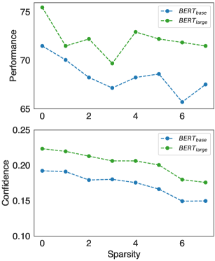
Figure 1: Performance and confidence on RTE (Bentivogli et al., 2009) of BERT_base and BERT_large at small sparsity levels. Task metric and output distribution variance are used as the measures of performance and confidence, respectively. Distribution variance is comparatively equivalent to distribution negative entropy as employed in Pereyra et al. (2017). Proof of the equivalence can be found in Appendix A.

Conventional studies (Sun et al., 2019; Jiao et al., 2020) mainly expect that the expressive knowledge would be well transferred, yet largely neglecting the existence of student-unfriendly knowledge. Recent attempts (Zhou et al., 2022; Zhao et al., 2022) are made to adapt the teacher to more student-friendly knowledge and have yielded performance gains. Based on these observations, we posit that over-parameterized LMs, on the one hand, can produce expressive knowledge due to over-parameterization, but on the other hand can also produce student-unfriendly knowledge due to over-confidence (Hinton et al., 2015; Pereyra et al., 2017). From a pilot study shown in Figure 1, we find that LMs of large scale tend to have a good performance and high confidence, and that both performance and confidence can be degraded through randomly sparsifying a small portion of parameters. This indicates that some parameters resulting in student-unfriendliness can be rather removed, to improve student-friendliness of the teacher without sacrificing too much its expressiveness.

Motivated by this finding, we propose a sparse teacher trick (in short, StarK ) under the guidance of an overall knowledgeable score for each teacher parameter, which accords not only with the expressiveness but also the student-friendliness of the parameter by interpolation. The aim is to retain the expressive parameters while removing the student-unfriendly ones. Specifically, we introduce a three-stage procedure consisting of 1) trial distillation, 2) parameter sparsification, and 3) actual distillation. The trial distillation distills the dense teacher to the student so that a trial student is obtained. The parameter sparsification first estimates the expressiveness score and student-friendliness score of each teacher parameter via feedbacks respectively from the teacher itself and the trial student, and then sparsifies the teacher by removing the parameters associated with adequately low interpolated knowledgeable scores. The actual distillation distills the sparsified teacher to the student so that an actual student is obtained, where the student is initialized in the same manner as that used in trial distillation following the commonly-used rewinding technique (Frankle and Carbin, 2019).

We conduct an extensive set of experiments on the GLUE benchmark. Experimental results demonstrate that the sparse teachers can be dense with knowledge and lead to a remarkable performance of students compared with a series of competitive baselines.

2 Background

2.1 BERT Architecture

The BERT (Devlin et al., 2019) is composed of several stacked encoder layers of transformers (Vaswani et al., 2017). There are two blocks in every encoder layer: a multi-head self-attention block (MHA) and a feed-forward network block (FFN), with a residual connection and a normalization layer around each.

Given an $l$-length sequence of $d$-dimensional input vectors $\mathbf{X}\in\mathbb{R}^{l\times d}$, the output of the MHA block with $A$ independent heads can be represented as:

$${\rm MHA}(\mathbf{X})$$

$$=\sum_{i=1}^{A}{\rm Attn}(\mathbf{X},\mathbf{W}_{Q}^{(i)},\mathbf{W}_{K}^{(i)},\mathbf{W}_{V}^{(i)})\mathbf{W}_{O}^{(i)},$$

where the $i$-th head is parameterized by $\mathbf{W}_{Q}^{(i)}$, $\mathbf{W}_{K}^{(i)}$, $\mathbf{W}_{V}^{(i)}\in\mathbb{R}^{d\times d_{A}}$, and $\mathbf{W}_{O}^{(i)}\in\mathbb{R}^{d_{A}\times d}$. On the other hand, the output of the FFN block is:

$${\rm FFN}(\mathbf{X})={\rm GELU}(\mathbf{X}\mathbf{W}_{1})\mathbf{W}_{2},$$

where two fully-connected layers are parameterized by $\mathbf{W}_{1}\in\mathbb{R}^{d\times d_{I}}$ and $\mathbf{W}_{2}\in\mathbb{R}^{d_{I}\times d}$ respectively.

2.2 Knowledge Distillation

Knowledge distillation (Hinton et al., 2015) aims to transfer the knowledge from a large-scale teacher to a smaller-scale student, which is originally proposed to supervise the student with the teacher logits. With its prevalence, a tremendous amount of work has been investigated to transfer various knowledge from the teacher to the student (Romero et al., 2015; Zagoruyko and Komodakis, 2017; Sun et al., 2019; Jiao et al., 2020; Park et al., 2021b; Li et al., 2020; Wang et al., 2020). PKD (Sun et al., 2019) introduces a patient distillation scheme where the student learns multiple intermediate layer representations and logits from the teacher. Moreover, attention distributions (Sun et al., 2020; Jiao et al., 2020; Li et al., 2020; Wang et al., 2020) and even high-order relations (Park et al., 2021b) are considered to further boost the performance.

Since a large capacity gap between the teacher and the student can lead to an inferior distillation quality, TAKD (Mirzadeh et al., 2020) proposes to insert teacher assistants of possible intermediate scales between the teacher and the student so that the gap is drawn closer (Zhang et al., 2022). More recently, teachers with student-friendly architectures have exactly showed the significance of student-friendliness (Park et al., 2021a). MetaKD (Zhou et al., 2022) adopts meta-learning to optimize the student-friendliness of the teacher according to the student preference. DKD (Zhao et al., 2022) decouples and amplifies student-friendly knowledge in contrast to others. Distinguished from these student-friendly teachers that are achieved by altering teacher scales, architectures, parameters or knowledge representations, our work, to our best knowledge, is the first one suggesting that teacher parameters can produce both student-friendly and student-unfriendly knowledge and aiming to find the sparse teacher with the best student-friendliness.

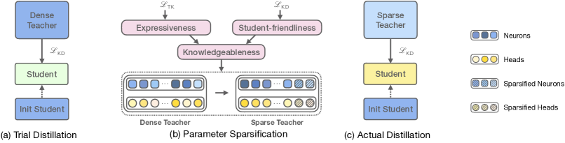
Figure 2: The overview of StarK. trial distillation distils a trial student from the dense teacher on a specific task. parameter sparsification sparsifies the parameters of the dense teacher that are associated with adequately low knowledgeable scores. actual distillation rewinds the trial distillation by replacing the dense teacher with the proposed sparse teacher.

2.3 Model Pruning

Model pruning is imposed to remove the less expressive parameters for model compression. Previous work applies either structured (Li et al., 2017; Luo et al., 2017; He et al., 2017; Yang et al., 2022) or unstructured pruning (Han et al., 2015; Park et al., 2017; Louizos et al., 2018; Lee et al., 2019) to transformers. Unstructured pruning focuses on pruning parameter-level parameters based on zero-order decisions derived from magnitudes (Gordon et al., 2020) or first-order decisions computed from both gradients and magnitudes (Sanh et al., 2020). In contrast, structured pruning prunes module-level parameters such like MHA heads (Michel et al., 2019) and FFN layers (Prasanna et al., 2020) guided by the expressive score (Michel et al., 2019). It is noteworthy that while some pruning methods leverage post-training pruning Hou et al. (2020), others can take advantage of training-time pruning Xia et al. (2022). Although training-time pruning can result in slightly better performance, it can consume much more time to meet a convergence. Our work mainly exploits structured pruning to obtain sparse teachers, yet also explores the use of unstructured pruning, in a post-training style.

3 Sparse Teacher Trick

Our trick involves three stages in the student learning procedure as shown in Figure 2. First, we distil a trial student from the dense teacher on a specific task (trial distillation). Then, we sparsify the parameters of the dense teacher that are associated with adequately low knowledgeable scores (parameter sparsification). Finally, rewinding is applied, where the student is set to the initialization exactly used in the trial distillation stage and is learned from the sparse teacher during (actual distillation).

3.1 Trial and Actual Distillations

Trial distillation and actual distillation share the same distillation regime. We employ the widely-used logits distillation (Hinton et al., 2015) as the distillation objective, as depicted below:

$$\mathcal{L}_{\sf KD}=-{\rm softmax}(\mathbf{z}^{t}/\tau)\log{\rm softmax}(\mathbf{z}^{s}/\tau),$$

$$\mathcal{L}_{\sf TK}=-\mathbf{y}\log\mathbf{y}^{s},$$

$$\mathcal{L}=\mathcal{L}_{\sf KD}+\alpha\cdot\mathcal{L}_{\sf TK},$$

where $\mathbf{z}^{t}$, $\mathbf{z}^{s}$ separately stand for logits of the teacher and student, and $\mathbf{y}^{s}$, $\mathbf{y}$ separately stand for prediction normalized probabilities of the student and ground-truth one-hot probabilities. Two subscripts ${\sf KD}$ and ${\sf TK}$ indicate distillation and task losses respectively. $\tau$ is a temperature controlling the smoothness the logits (Hinton et al., 2015), and $\alpha$ is a term balancing two losses.

The trial distillation and actual distillation also reuse the initialization of the student for better convergence, which is known as rewinding technique (Frankle and Carbin, 2019).

3.2 Parameter Sparsification

For parameter sparsification, we design a knowledgeable score, which is essentially an interpolation of the already-proposed expressive score (Molchanov et al., 2017) and our proposed student-friendly score, to measure the knowledgeableness of each teacher parameter. Thanks to the knowledgeable score, we can safely exclude student-unfriendly parameters without harming expressive parameters too much.

We mainly sparsify the attention heads of MHA blocks and intermediate neurons of FFN blocks in the teacher. Following the literature on structured pruning in a post-training style (Michel et al., 2019; Hou et al., 2020), we attach a set of variables $\xi^{(i)}$ and $\nu$ to the attention heads and the intermediate neurons, to record the parameter sensitivities for a specific task through accumulated absolute gradients, as shown below:

$${\rm MHA}^{\circ}(\mathbf{X})$$

$$=\sum_{i=1}^{A}\xi^{(i)}{\rm Attn}(\mathbf{X},\mathbf{W}_{Q}^{(i)},\mathbf{W}_{K}^{(i)},\mathbf{W}_{V}^{(i)})\mathbf{W}_{O}^{(i)},$$

$${\rm FFN}^{\circ}(\mathbf{X})={\rm GELU}(\mathbf{X}\mathbf{W}_{1}){\rm diag}(\nu)\mathbf{W}_{2},$$

where $\xi^{(i)}\equiv 1$ and $\nu\equiv\mathbf{1}^{d_{I}}$. We set the values of the $\xi^{(i)}$ and $\nu$ to ones to ensure the functionalities of corresponding heads and neurons are retained.

The implementation is mathematically equivalent to the prevalent first-order taylor expansion of the absolute variation between before and after removing a module (i.e., a head or a neuron) akin to Molchanov et al. (2017). Take the $i$-th attention head as an example, its parameter sensitivity can be written as:

$$\left|\frac{\partial\mathcal{L}}{\partial\xi^{(i)}}\right|=\left|\frac{\partial\mathcal{L}}{\partial\xi^{(i)}\mathbf{O}^{(i)}}\frac{\partial\xi^{(i)}\mathbf{O}^{(i)}}{\partial\xi^{(i)}}\right|=\left|\frac{\partial\mathcal{L}}{\partial\mathbf{O}^{(i)}}\mathbf{O}^{(i)}\right|$$

$$\approx\left|(\mathcal{L}_{\mathbf{0}}+\frac{\partial\mathcal{L}}{\partial\mathbf{O}^{(i)}}(\mathbf{O}^{(i)}-\mathbf{0})+\mathbf{r})-\mathcal{L}_{\mathbf{0}}\right|$$

$$=\left|\mathcal{L}-\mathcal{L}_{\mathbf{0}}\right|,$$

where $\mathcal{L}$ stands for an arbitrary objective with abuse of notation, and $\mathbf{O}^{(i)}$ is utilized for $i$-th attention head output. $\mathcal{L}_{\mathbf{0}}$ actually means $\mathcal{L}|_{\mathbf{O}^{(i)}=\mathbf{0}}$, and $\mathbf{r}$ represents residuals in taylor expansion.

Note that our trick can be flexibly extended to a training-time style (Xia et al., 2022) or unstructured pruning, which will be discussed in our experiments.

Expressiveness.

The expressiveness of the teacher is tied to the expressiveness score. A higher expressiveness score indicates that the corresponding parameter has bigger contribution towards the performance. Concretely, the expressiveness scores of the attention heads in MHA and the intermediate neurons in FFN can be depicted as:

$$\mathbb{P}_{\sf head}^{(i)} =\mathbb{E}_{\mathcal{D}}\left|\frac{\partial\mathcal{L}_{\sf TK}}{\partial\xi^{(i)}}\right|,$$

$$\mathbb{P}_{\sf neuron} =\mathbb{E}_{\mathcal{D}}\left|\frac{\partial\mathcal{L}_{\sf TK}}{\partial{\rm diag}(\nu)}\right|,$$

where $\mathcal{D}$ is a data distribution, and $\mathcal{L}_{\sf TK}$ is the task loss of the teacher. $\mathbb{E}$ represents expectation.

Student-friendliness.

Likewise, the student-friendliness of the teacher can be described as student-friendliness scores, which are approximated from distillation loss of the trial distillation.

$$\mathbb{Q}_{\sf head}^{(i)} =\mathbb{E}_{\mathcal{D}}\left|\frac{\partial\mathcal{L}_{\sf KD}}{\partial\xi^{(i)}}\right|,$$

$$\mathbb{Q}_{\sf neuron} =\mathbb{E}_{\mathcal{D}}\left|\frac{\partial\mathcal{L}_{\sf KD}}{\partial{\rm diag}(\nu)}\right|,$$

where $\mathcal{L}_{\sf KD}$ is the distillation loss as computed with the trial student from the trial distillation. Accordingly, the higher the student-friendliness score is, the more friendliness the teacher offers.

Referring to Molchanov et al. (2017), we normalize the expressiveness and student-friendliness scores with $\ell_{2}$ norm. In view that the teacher needs to balance the expressiveness and student-friendliness, we introduce a coefficient $\lambda$ to quantify the tradeoff. Therefore, the knowledgeable score can be written in an interpolated form:

$$\mathbb{I}_{\sf head}^{(i)} =\lambda\cdot\mathbb{P}_{\sf head}^{(i)}+(1-\lambda)\cdot\mathbb{Q}_{\sf head}^{(i)},$$

$$\mathbb{I}_{\sf neuron} =\lambda\cdot\mathbb{P}_{\sf neuron}+(1-\lambda)\cdot\mathbb{Q}_{\sf neuron},$$

Parameter sparsification sparsifies the parameters in the teacher with adequately low knowledgeable scores. The adequacy is met by enumerating diverse sparsity levels and obtaining the one leading to the best student during the actual distillation.

4 Experiments

4.1 Data & Metrics

Dataset	#Train exam.	#Dev exam.	Max. length	Metric
SST-2	67K	0.9K	64	Accuracy
MRPC	3.7K	0.4K	128	F1
STS-B	7K	1.5K	128	Spearman Correlation
QQP	364K	40K	128	F1
MNLI-m/mm	393K	20K	128	Accuracy
QNLI	105K	5.5K	128	Accuracy
RTE	2.5K	0.3K	128	Accuracy

Table 1: The statistics, maximum sequence lengths, and metrics of the GLUE benchmark.

We evaluate our approach on GLUE benchmark (Wang et al., 2019) that contains a collection of NLU tasks, including CoLA (Warstadt et al., 2019) for linguistic acceptability, SST-2 (Socher et al., 2013) for sentiment analysis, MRPC (Dolan and Brockett, 2005), QQP and STS-B (Cer et al., 2017) for paraphrase similarity matching, MNLI (Williams et al., 2018), QNLI (Rajpurkar et al., 2016) and RTE (Dagan et al., 2005; Haim et al., 2006; Giampiccolo et al., 2007; Bentivogli et al., 2009) for natural language inference. Note that we exclude CoLA (Warstadt et al., 2019) on which general knowledge distillation methods transfer knowledge poorly (Xia et al., 2022).

Accuracy is adopted as the evaluation metric for MNLI-m, MNLI-mm, QNLI, RTE and SST-2, and F1-score is used for MRPC, QQP. The Spearman correlation is used for STS-B. We also report the Average results on development sets of all datasets. We display the statistics of GLUE in Table 1.

4.2 Implementation & Baselines

We conduct experiments on an Nvidia V100. AdamW (Loshchilov and Hutter, 2019) is applied as the optimizer. We search the learning rate within {1, 2, 3}$\times$10^-5 and the batch size within {16, 32}. All training procedures are carried out within 10 epochs, with an early-stopping. We empirically find that, when temperature $\tau$ is 2.0 and distillation balance $\alpha$ is 1.0, reasonable performance is attained. The optimal sparsity is searched within {10%, 20%, 30%, 40%, 50%, 60%, 70%, 80%, 90%}. Knowledgeableness tradeoff $\lambda$ is set to 0.5 for acceptable performance and its impact on the performance will be discussed later.

We finetune the original BERT as the teacher and distil it to the student of a smaller scale initialized by dropping 2/3 layers or pruning 70% parameters (with above-mentioned expressiveness pruning) of the teacher, which is initialized from the teacher. We first directly finetune the student as a solid baseline (FT). Then we compare our method to conventional baselines, such as KD Hinton et al. (2015), PKD Sun et al. (2019), CKD Park et al. (2021b), and DynaBERT Hou et al. (2020). Further, we compare our method to student-friendly baselines, including TAKD that employs a reasonable assistant (Mirzadeh et al., 2020), MetaKD (Zhou et al., 2022) that adapts the teacher with the student feedback, and DKD (Zhao et al., 2022) that amplifies the student-friendly knowledge.

4.3 Main Comparison

Method	MNLI-m Acc	MNLI-mm Acc	MRPC F1	QNLI Acc	QQP F1	RTE Acc	STSB SpCorr	SST-2 Acc	Average
BERTbase	84.9	84.9	91.2	91.7	88.4	71.5	88.3	93.8	86.8
layer-dropped student
FT4	77.5	77.7	86.0	85.3	86.1	65.0	86.5	89.5	81.7
KD4	77.7	77.7	86.9	85.1	86.1	65.3	86.4	89.6	81.8
PKD4	77.7	77.7	87.6	85.0	86.0	65.3	86.4	89.9	82.0
CKD4	77.7	77.9	87.2	85.0	86.2	64.6	86.4	89.6	81.8
MetaKD4	\	\	85.1	\	\	63.9	86.5	89.5	\
DKD4	77.9	78.0	86.9	84.8	86.0	66.3	86.5	88.8	81.9
TAKD4	77.1	77.3	87.2	84.5	86.3	67.9	86.7	89.9	82.1
StarK4	78.8	79.0	87.4	85.7	86.5	67.5	87.2	90.6	82.8
§	40%	50%	50%	50%	30%	60%	40%	50%	46%
parameter-pruned student
FT30%	82.0	82.6	88.5	89.5	87.7	69.0	87.2	91.9	84.8
KD30%	82.5	82.4	89.1	89.5	87.8	69.3	87.0	91.9	84.9
PKD30%	82.5	82.8	89.5	89.9	88.0	68.6	86.4	91.9	84.9
DynaBERT30%	81.5	82.8	87.4	89.1	86.6	68.1	87.2	90.3	84.1
DKD30%	82.4	82.4	88.4	89.6	87.7	70.4	87.0	91.9	85.0
TAKD30%	82.7	82.3	89.1	89.8	87.8	68.6	87.6	91.9	85.0
StarK30%	82.8	82.9	89.4	90.0	87.8	69.7	87.9	92.2	85.3
§	30%	20%	30%	70%	40%	20%	30%	40%	35%

Table 2: The results of main comparison on GLUE development set. The best results on datasets are boldfaced. § is the optimal sparsity on each dataset. *₄ and *_30% mean the student is initialized by dropping 2/3 layers or pruning 70% parameters of the teacher. StarK₄ and StarK_30% exactly mean KD₄ and KD_30% w/ StarK. We only report MetaKD on small datasets due to limited resources, and DynaBERT without data augmentation due to unavailable augmented data.

Table 2 shows the main experimental results. We can observe that StarK has a significant performance gain by comparing StarK with the original KD. Numerically, the absolute improvements brought by StarK are 1.0% and 0.4% in term of Average. This result implies that sparse teachers can be dense with knowledge. On another note, this possibly indicates a good teacher should be a modest one. Moreover, StarK achieves 0.7% and 0.3% absolute improvements when compared to the competitive TAKD, illustrating that sparse teachers can be more expressive and student-friendly, thereby more knowledgeable to the student than teacher assistants. It seems that student-friendly baselines can only realize a comparable performance to the conventional baselines. We argue this is not the case when student-friendly baselines, say DKD, are armed with advanced distillation objectives, say PKD. Also note that the performances of MetaKD and DynaBERT are lower than those originally reported, as the original work either initialized the student from a pretrained LM of the same scale or utilized extra augmented data.

4.4 Analyses

Knowledgeableness Tradeoff

To investigate the impact of the tradeoff between expressiveness and student-friendliness, we conduct more experiments by varying $\lambda$ values. Figure 3 illustrates the performance variation along with the change of $\lambda$. The performance generally exhibits a concave curvature, which hints that the sparsification of the teacher does face with a tradeoff between expressiveness and student-friendliness, and an ideal $\lambda$ should be not too large or too small.

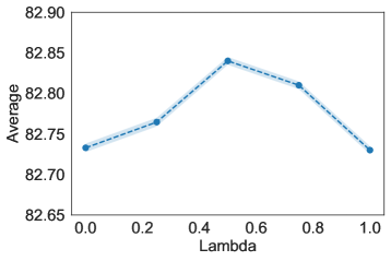
Figure 3: Performance of StarK₄ with different $\lambda$.

Scalability

Method	MNLI-m Acc	MNLI-mm Acc	MRPC F1	QNLI Acc	QQP Acc	RTE Acc	STSB SpCorr	SST-2 Acc	Average
BERTlarge	86.6	86.1	92.3	92.2	89.0	75.5	89.9	93.9	88.2
KD8	78.9	79.5	84.9	86.1	86.4	63.9	85.6	90.5	82.0
StarK8	79.4	80.5	85.0	86.3	87.0	65.7	88.7	90.9	82.9
§	30%	20%	90%	10%	30%	60%	20%	20%	35%
BERTbase	84.9	84.9	91.2	91.7	88.4	71.5	88.3	93.8	86.8
KD2	73.2	72.8	82.9	78.9	83.5	58.5	46.5	86.8	72.9
StarK2	73.9	74.3	83.1	80.4	83.8	57.8	48.6	88.1	73.7
§	50%	50%	30%	50%	30%	40%	30%	40%	40%

Table 3: The results of scalability to larger teachers and smaller students.

To examine the scalability of StarK to larger teachers (i.e., BERT_large) and smaller students (i.e., *₂), where distillation methods can in fact suffer more severely from student-unfriendliness, we distil from BERT_large to an eight-layer student with KD and StarK, and also distill from BERT_base to an two-layer student. The results shown in Table 3 suggest that StarK works well on large teachers and smaller students, and the capacity gap between large teachers and small students can be drawn closer by selecting a sparse teacher. However, the eight-layer student distilled from BERT_large performs only slightly better than the four-layer student distilled from BERT_base even with StarK (see Table 2). With  1/3 parameters, StarK₄ can achieve 95% performance of BERT_base, and such 95%/33% scale-performance tradeoff is acceptable in real-world applications. In contrast, the two-layer student can only get a 85%/17% tradeoff, limiting its practical usage.

Stage	Train time on MNLI
trial distillation	$\sim$2.5h
actual distillation	$\sim$7h

Table 4: The training time consumed during trial distillation and actual distillation stages.

Training Efficiency

StarK indeed requires more training time compared to KD due to the exhaustive search during the actual distillation stage. However, it dose not introduce heavy compute since the search mainly involves additional distillations with sparsified teachers that are smaller than the original teacher. Table 4 indicates that actual distillation consumes not that much more training time than trial distillation. Hence, we believe the tradeoff between training time and student performance, along with training efficiency, is acceptable.

Pluggability

Method	MNLI-m Acc	MNLI-mm Acc	MRPC F1	QNLI Acc	QQP Acc	RTE Acc	STSB SpCorr	SST-2 Acc	Average
BERTbase	84.9	84.9	91.2	91.7	88.4	71.5	88.3	93.8	86.8
KD4	77.7	77.7	86.9	85.1	86.1	65.3	86.4	89.6	81.8
w/ StarK	78.8	79.0	87.4	85.7	86.5	67.5	87.2	90.6	82.8
PKD4	77.7	77.7	87.6	85.0	86.0	65.3	86.4	89.9	82.0
w/ StarK	78.8	79.1	87.7	85.9	86.6	66.8	87.2	90.1	82.8
CKD4	77.7	77.9	87.2	85.0	86.2	64.6	86.4	89.6	81.8
w/ StarK	78.8	79.0	87.6	86.4	86.5	66.4	87.2	90.4	82.8

Table 5: The results of pluggability to baselines.

We also show StarK is pluggable to any distillation methods since it is orthogonal to existing paradigms. We hence plug StarK to our baselines KD, PKD, and CKD to distil a four-layer student from BERT_base. As in Table 5, we observe that StarK has universal pluggability to regarded baselines, averagely improving the absolute performance by 0.9%.

Unstructured Pruning

As aforementioned, StarK can be flexibly applied with unstructured pruning. For unstructured pruning, we derive the expressiveness and student-friendliness scores in the same way as that used in our structured StarK, except the recording variables are attached to parameters rather than modules like heads. The results in Table 6 verify that StarK with unstructured pruning is slightly worse that StarK with structured pruning, yet it still outperforms KD. Thus, StarK is capable of unstructured pruning.

Method	MNLI-m Acc	MNLI-mm Acc	MRPC F1	QNLI Acc	QQP Acc	RTE Acc	STSB SpCorr	SST-2 Acc	Average
BERTbase	84.9	84.9	91.2	91.7	88.4	71.5	88.3	93.8	86.8
KD4	77.7	77.7	86.9	85.1	86.1	65.3	86.4	89.6	81.8
StarK4	78.8	79.0	87.4	85.7	86.5	67.5	87.2	90.6	82.8
StarK4*	79.0	79.0	87.4	85.3	86.8	66.1	87.3	89.8	82.6

Table 6: The results of compatibility with unstructured pruning. ^* indicates that unstructured pruning is otherwise used.

Automatic StarK

Method	MNLI-m Acc	MNLI-mm Acc	MRPC F1	QNLI Acc	QQP Acc	RTE Acc	STSB SpCorr	SST-2 Acc	Average
StarK4	78.8	79.0	87.4	85.7	86.5	67.5	87.2	90.6	82.8
§	40%	50%	50%	50%	30%	60%	40%	50%	46%
StarK-Auto4	78.1	79.0	86.6	85.7	86.0	67.5	87.2	90.0	82.6
§	47%	51%	35%	46%	44%	42%	38%	38%	43%

Table 7: The results of StarK-Auto.

An issue with StarK is that the optimal sparsity is obtained by exhaustively enumerating all candidate sparsity levels, leading to some level of training-inefficiency. To address it, we explore an alternative algorithm to get the optimal sparsity so that StarK is enabled with a pursued automatic property. To this end, an attentive solution is proposed based on a surprising observation that a sparse teacher under the guidance of randomness (denoted as StarK-Rand₄) can achieve a promising Average score of 82.5%, whereas the scores for KD₄ and StarK₄ are correspondingly 81.8% and 82.8%. This weird phenomenon drives us to put forward a proposition.

Assumption 1.

Both expressiveness and student-friendliness scores are densely located at their clusters, where the cluster center of student-friendliness scores owns a smaller magnitude than that of expressiveness scores.

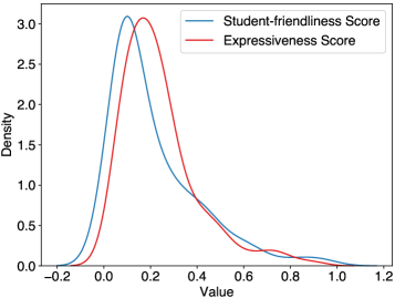
Figure 4: Density of expressiveness and student-friendliness scores of BERT_base attention heads finetuned on MRPC (Dolan and Brockett, 2005). Intermediate neurons share similar characteristics, which are supplied in Appendix B.

The assumption is intuitively verified in Figure 4. When random pruning is conducted, firstly the probability of sparsifying a student-unfriendly parameter is high, and secondly the joint probability of sparsifying a student-unfriendly and inexpressive parameter is higher than that of sparsifying a student-unfriendly yet expressive parameter. Therefore, the performance of StarK-Rand is guaranteed with certain probability by Assumption 1. However, we argue StarK is always a more robust choice than StarK-Rand.

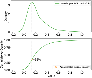
Figure 5: Density and cumulative density of knowledgeableness scores of BERT_base attention heads finetuned on MRPC (Dolan and Brockett, 2005). Intermediate neurons share similar characteristics, which are supplied in Appendix B. Full results on all tasks are supplied in Appendix C.

A follow-up observation is that StarK-Rand₄ expects a smaller average sparsity (25%) than StarK₄ does (46%). It is easy to understand that the more parameters are sparsified, the lower probability above the performance guarantee will hold, though. The evident phenomenon inspires us to make another assumption.

Assumption 2.

An optimal sparsity is positively correlated to the first density peak of a sparsification sequence.

The assumption is illustrated in Figure 5. Since StarK-Rand sparsifies parameters at random, it will have a small optimal sparsity as a consequence of meeting the first density peak very early. For StarK enjoys a sparsification sequence with only one density peak, its optimal sparsity can be automatically estimated (denoted as StarK-Auto) through Assumption 2. Experimental results can be found in Table 7, where StarK-Auto approximates StarK in term of the Average metric. Nevertheless, we argue it is the last to use StarK-Auto otherwise for an extremely low practical compute as the performance can suffer a subtle drop.

5 Conclusions

In this paper, we validate that sparse teachers can be dense with knowledge under the guidance of our designed knowledgeable score. The idea of the sparse teacher is motivated from a pilot study, and the knowledgeable score is carefully crafted to make sure that the student-unfriendly knowledge can be reduced without hurting too much the expressive knowledge. Extensive experimental results on the GLUE benchmark support our claim to a large degree.

Limitations

StarK can be further explored under two additional settings: 1) in a task-agnostic setting (e.g., MiniLM) and 2) on large LMs (e.g., BERT_large). Moreover, our attentive automatic solution for StarK can be enhanced so that its performance can at least match the original performance.

Appendix A Comparative Equivalence of Distribution Variance and Negative Entropy

Theorem 1.

For any two distributions $\mathbf{y}$ and $\mathbf{y}^{\prime}$, the negative entropy difference between them can be approximated by their variance difference.

Proof.

$$-\mathcal{H}(\mathbf{y})-(-\mathcal{H}(\mathbf{y}^{\prime}))$$

$$=\sum_{i}\mathbf{y}_{i}\log\mathbf{y}_{i}-\sum_{i}\mathbf{y}^{\prime}_{i}\log\mathbf{y}^{\prime}_{i}$$

$$\approx\sum_{i}(\mathbf{y}_{i}-1)+\frac{1}{2}(\mathbf{y}_{i}-1)^{2}+\mathbf{r}$$

$$\qquad-\sum_{i}(\mathbf{y}_{i}^{\prime}-1)+\frac{1}{2}(\mathbf{y}_{i}^{\prime}-1)^{2}+\mathbf{r}$$

$$=\sum_{i}-(\mathbf{y}_{i}-\mathbf{y}_{i}^{\prime})+\frac{1}{2}(\mathbf{y}_{i}^{2}-\mathbf{y}_{i}^{\prime 2})$$

$$=\sum_{i}\frac{1}{2}((\mathbf{y}_{i}-\bar{\mathbf{y}})^{2}-(\mathbf{y}_{i}^{\prime}-\bar{\mathbf{y}}^{\prime})^{2})$$

$$\propto\sum_{i}(\mathbf{y}_{i}-\bar{\mathbf{y}})^{2}-\sum_{i}(\mathbf{y}_{i}^{\prime}-\bar{\mathbf{y}}^{\prime})^{2}$$

$$=\mathcal{V}(\mathbf{y})-\mathcal{V}(\mathbf{y}^{\prime}).$$

∎

Corollary 1.

Distribution variance, when taken as the measure of confidence, is comparatively equivalent to distribution negative entropy.

Appendix B Density of Scores of BERT_base Intermediate Neurons on MRPC

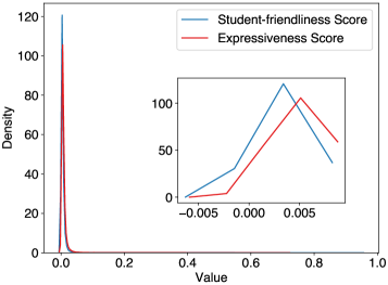
Figure 6: Density of expressiveness and student-friendliness scores of BERT_base intermediate neurons finetuned on MRPC (Dolan and Brockett, 2005).

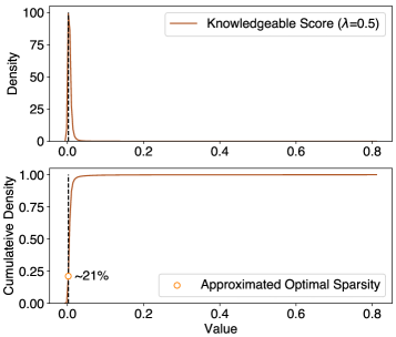
Figure 7: Density and cumulative density of knowledgeableness scores of BERT_base intermediate neurons finetuned on MRPC (Dolan and Brockett, 2005).

Appendix C Density of Scores of BERT_base Attention Heads on GLUE

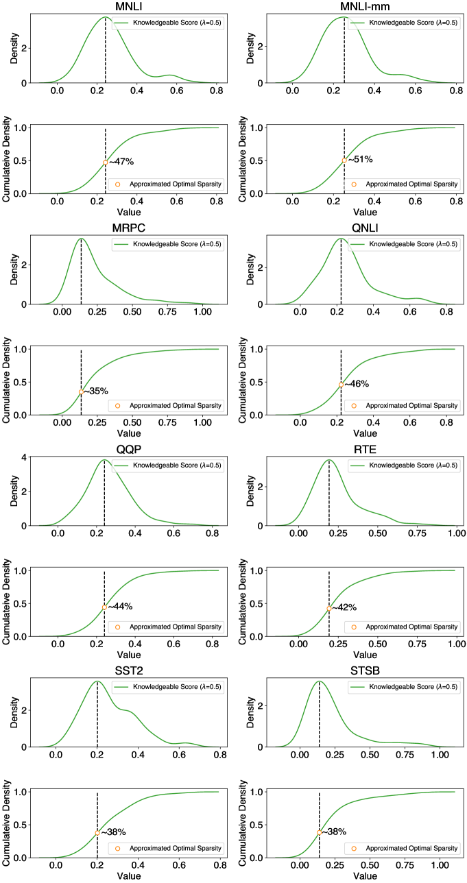
Figure 8: Density and cumulative density of knowledgeableness scores of BERT_base attention heads finetuned on GLUE.

References

- Bentivogli et al. (2009) Luisa Bentivogli, Bernardo Magnini, Ido Dagan, Hoa Trang Dang, and Danilo Giampiccolo. 2009. The fifth PASCAL recognizing textual entailment challenge. In TAC.
- Cer et al. (2017) Daniel M. Cer, Mona T. Diab, Eneko Agirre, Iñigo Lopez-Gazpio, and Lucia Specia. 2017. Semeval-2017 task 1: Semantic textual similarity multilingual and crosslingual focused evaluation. In SemEval@ACL, pages 1–14.
- Dagan et al. (2005) Ido Dagan, Oren Glickman, and Bernardo Magnini. 2005. The PASCAL recognising textual entailment challenge. In PASCAL, MLCW, volume 3944, pages 177–190.
- Devlin et al. (2019) Jacob Devlin, Ming-Wei Chang, Kenton Lee, and Kristina Toutanova. 2019. BERT: pre-training of deep bidirectional transformers for language understanding. In NAACL, pages 4171–4186.
- Dolan and Brockett (2005) William B. Dolan and Chris Brockett. 2005. Automatically constructing a corpus of sentential paraphrases. In IWP@IJCNLP.
- Frankle and Carbin (2019) Jonathan Frankle and Michael Carbin. 2019. The lottery ticket hypothesis: Finding sparse, trainable neural networks. In ICLR.
- Ganesh et al. (2021) Prakhar Ganesh, Yao Chen, Xin Lou, Mohammad Ali Khan, Yin Yang, Hassan Sajjad, Preslav Nakov, Deming Chen, and Marianne Winslett. 2021. Compressing large-scale transformer-based models: A case study on BERT. TACL, 9:1061–1080.
- Giampiccolo et al. (2007) Danilo Giampiccolo, Bernardo Magnini, Ido Dagan, and Bill Dolan. 2007. The third PASCAL recognizing textual entailment challenge. In ACL-PASCAL@ACL, pages 1–9.
- Gordon et al. (2020) Mitchell A. Gordon, Kevin Duh, and Nicholas Andrews. 2020. Compressing BERT: studying the effects of weight pruning on transfer learning. In RepL4NLP@ACL, pages 143–155.
- Haim et al. (2006) R Bar Haim, Ido Dagan, Bill Dolan, Lisa Ferro, Danilo Giampiccolo, Bernardo Magnini, and Idan Szpektor. 2006. The second pascal recognising textual entailment challenge. In PASCAL, volume 7.
- Han et al. (2015) Song Han, Jeff Pool, John Tran, and William J. Dally. 2015. Learning both weights and connections for efficient neural network. In NeurIPS, pages 1135–1143.
- He et al. (2017) Yihui He, Xiangyu Zhang, and Jian Sun. 2017. Channel pruning for accelerating very deep neural networks. In ICCV, pages 1398–1406.
- Hinton et al. (2015) Geoffrey E. Hinton, Oriol Vinyals, and Jeffrey Dean. 2015. Distilling the knowledge in a neural network. arXiv, 1503.02531.
- Hou et al. (2020) Lu Hou, Zhiqi Huang, Lifeng Shang, Xin Jiang, Xiao Chen, and Qun Liu. 2020. Dynabert: Dynamic BERT with adaptive width and depth. In NeurIPS.
- Jiao et al. (2020) Xiaoqi Jiao, Yichun Yin, Lifeng Shang, Xin Jiang, Xiao Chen, Linlin Li, Fang Wang, and Qun Liu. 2020. Tinybert: Distilling BERT for natural language understanding. In Findings of EMNLP, volume EMNLP 2020, pages 4163–4174.
- Lee et al. (2019) Namhoon Lee, Thalaiyasingam Ajanthan, and Philip H. S. Torr. 2019. Snip: single-shot network pruning based on connection sensitivity. In ICLR.
- Li et al. (2017) Hao Li, Asim Kadav, Igor Durdanovic, Hanan Samet, and Hans Peter Graf. 2017. Pruning filters for efficient convnets. In ICLR.
- Li et al. (2020) Jianquan Li, Xiaokang Liu, Honghong Zhao, Ruifeng Xu, Min Yang, and Yaohong Jin. 2020. BERT-EMD: many-to-many layer mapping for BERT compression with earth mover’s distance. In EMNLP, pages 3009–3018.
- Liu et al. (2019) Yinhan Liu, Myle Ott, Naman Goyal, Jingfei Du, Mandar Joshi, Danqi Chen, Omer Levy, Mike Lewis, Luke Zettlemoyer, and Veselin Stoyanov. 2019. Roberta: A robustly optimized BERT pretraining approach. arXiv, 1907.11692.
- Loshchilov and Hutter (2019) Ilya Loshchilov and Frank Hutter. 2019. Decoupled weight decay regularization. In ICLR.
- Louizos et al. (2018) Christos Louizos, Max Welling, and Diederik P. Kingma. 2018. Learning sparse neural networks through l_0 regularization. In ICLR.
- Luo et al. (2017) Jian-Hao Luo, Jianxin Wu, and Weiyao Lin. 2017. Thinet: A filter level pruning method for deep neural network compression. In ICCV, pages 5068–5076.
- Michel et al. (2019) Paul Michel, Omer Levy, and Graham Neubig. 2019. Are sixteen heads really better than one? In NeurIPS, pages 14014–14024.
- Mirzadeh et al. (2020) Seyed-Iman Mirzadeh, Mehrdad Farajtabar, Ang Li, Nir Levine, Akihiro Matsukawa, and Hassan Ghasemzadeh. 2020. Improved knowledge distillation via teacher assistant. In AAAI, pages 5191–5198.
- Molchanov et al. (2017) Pavlo Molchanov, Stephen Tyree, Tero Karras, Timo Aila, and Jan Kautz. 2017. Pruning convolutional neural networks for resource efficient inference. In ICLR.
- Park et al. (2021a) Dae Young Park, Moon-Hyun Cha, Changwook Jeong, Daesin Kim, and Bohyung Han. 2021a. Learning student-friendly teacher networks for knowledge distillation. In NeurIPS, pages 13292–13303.
- Park et al. (2021b) Geondo Park, Gyeongman Kim, and Eunho Yang. 2021b. Distilling linguistic context for language model compression. In EMNLP, pages 364–378.
- Park et al. (2017) Jongsoo Park, Sheng R. Li, Wei Wen, Ping Tak Peter Tang, Hai Li, Yiran Chen, and Pradeep Dubey. 2017. Faster cnns with direct sparse convolutions and guided pruning. In ICLR.
- Pereyra et al. (2017) Gabriel Pereyra, George Tucker, Jan Chorowski, Lukasz Kaiser, and Geoffrey E. Hinton. 2017. Regularizing neural networks by penalizing confident output distributions. In ICLR.
- Prasanna et al. (2020) Sai Prasanna, Anna Rogers, and Anna Rumshisky. 2020. When BERT plays the lottery, all tickets are winning. In EMNLP, pages 3208–3229.
- Raffel et al. (2020) Colin Raffel, Noam Shazeer, Adam Roberts, Katherine Lee, Sharan Narang, Michael Matena, Yanqi Zhou, Wei Li, and Peter J. Liu. 2020. Exploring the limits of transfer learning with a unified text-to-text transformer. JMLR, 21:140:1–140:67.
- Rajpurkar et al. (2016) Pranav Rajpurkar, Jian Zhang, Konstantin Lopyrev, and Percy Liang. 2016. Squad: 100, 000+ questions for machine comprehension of text. In EMNLP, pages 2383–2392.
- Romero et al. (2015) Adriana Romero, Nicolas Ballas, Samira Ebrahimi Kahou, Antoine Chassang, Carlo Gatta, and Yoshua Bengio. 2015. Fitnets: Hints for thin deep nets. In ICLR.
- Sanh et al. (2020) Victor Sanh, Thomas Wolf, and Alexander M. Rush. 2020. Movement pruning: Adaptive sparsity by fine-tuning. In NeurIPS.
- Socher et al. (2013) Richard Socher, Alex Perelygin, Jean Wu, Jason Chuang, Christopher D. Manning, Andrew Y. Ng, and Christopher Potts. 2013. Recursive deep models for semantic compositionality over a sentiment treebank. In EMNLP, pages 1631–1642.
- Sun et al. (2019) Siqi Sun, Yu Cheng, Zhe Gan, and Jingjing Liu. 2019. Patient knowledge distillation for BERT model compression. In EMNLP, pages 4322–4331.
- Sun et al. (2020) Zhiqing Sun, Hongkun Yu, Xiaodan Song, Renjie Liu, Yiming Yang, and Denny Zhou. 2020. Mobilebert: a compact task-agnostic BERT for resource-limited devices. In ACL, pages 2158–2170.
- Vaswani et al. (2017) Ashish Vaswani, Noam Shazeer, Niki Parmar, Jakob Uszkoreit, Llion Jones, Aidan N. Gomez, Lukasz Kaiser, and Illia Polosukhin. 2017. Attention is all you need. In NeurIPS, pages 5998–6008.
- Wang et al. (2019) Alex Wang, Amanpreet Singh, Julian Michael, Felix Hill, Omer Levy, and Samuel R. Bowman. 2019. GLUE: A multi-task benchmark and analysis platform for natural language understanding. In ICLR.
- Wang et al. (2020) Wenhui Wang, Furu Wei, Li Dong, Hangbo Bao, Nan Yang, and Ming Zhou. 2020. Minilm: Deep self-attention distillation for task-agnostic compression of pre-trained transformers. In NeurIPS.
- Warstadt et al. (2019) Alex Warstadt, Amanpreet Singh, and Samuel R. Bowman. 2019. Neural network acceptability judgments. TACL, 7:625–641.
- Williams et al. (2018) Adina Williams, Nikita Nangia, and Samuel R. Bowman. 2018. A broad-coverage challenge corpus for sentence understanding through inference. In NAACL-HLT, pages 1112–1122.
- Xia et al. (2022) Mengzhou Xia, Zexuan Zhong, and Danqi Chen. 2022. Structured pruning learns compact and accurate models. In ACL, pages 1513–1528.
- Yang et al. (2022) Yi Yang, Chen Zhang, Benyou Wang, and Dawei Song. 2022. Doge tickets: Uncovering domain-general language models by playing lottery tickets. In NLPCC, volume 13551 of Lecture Notes in Computer Science, pages 144–156.
- Zagoruyko and Komodakis (2017) Sergey Zagoruyko and Nikos Komodakis. 2017. Paying more attention to attention: Improving the performance of convolutional neural networks via attention transfer. In ICLR.
- Zhang et al. (2022) Chen Zhang, Yang Yang, Qifan Wang, Jiahao Liu, Jingang Wang, Wei Wu, and Dawei Song. 2022. Autodisc: Automatic distillation schedule for large language model compression. arXiv, 2205.14570.
- Zhao et al. (2022) Borui Zhao, Quan Cui, Renjie Song, Yiyu Qiu, and Jiajun Liang. 2022. Decoupled knowledge distillation. arXiv, 2203.08679.
- Zhou et al. (2022) Wangchunshu Zhou, Canwen Xu, and Julian J. McAuley. 2022. BERT learns to teach: Knowledge distillation with meta learning. In ACL, pages 7037–7049.