Data Selection: A Surprisingly Effective and General Principle for Building Small Interpretable Models

Abstract

We present convincing empirical evidence for an effective and general strategy for building accurate small models. Such models are attractive for interpretability and also find use in resource-constrained environments. The strategy is to learn the training distribution instead of using data from the test distribution. The distribution learning algorithm is not a contribution of this work; we highlight the broad usefulness of this simple strategy on a diverse set of tasks, and as such these rigorous empirical results are our contribution. We apply it to the tasks of (1) building cluster explanation trees, (2) prototype-based classification, and (3) classification using Random Forests, and show that it improves the accuracy of weak traditional baselines to the point that they are surprisingly competitive with specialized modern techniques.

This strategy is also versatile wrt the notion of model size. In the first two tasks, model size is identified by number of leaves in the tree and the number of prototypes respectively. In the final task involving Random Forests the strategy is shown to be effective even when model size is determined by more than one factor: number of trees and their maximum depth.

Positive results using multiple datasets are presented that are shown to be statistically significant. These lead us to conclude that this strategy is both effective, i.e, leads to significant improvements, and general, i.e., is applicable to different tasks and model families, and therefore merits further attention in domains that require small accurate models.

1 Introduction

The application of Machine Learning to various domains often leads to specialized requirements. One such requirement is small model size, which is useful in the following scenarios:

1. Interpretability: It is easier for humans to parse models when they are small. For example, a decision tree with a depth of 5 is likely easier to understand than one with a depth of 50. Multiple user studies have established model size as an important factor for interpretability (Feldman 2000; Lage et al. 2019; Poursabzi-Sangdeh et al. 2021). This is also true for explanations that are models, where post-hoc interpretability is desired, e.g., local linear models with a small number of non-zero coefficients as in LIME (Ribeiro, Singh, and Guestrin 2016) or cluster explanation trees with a low number of leaves (Moshkovitz et al. 2020; Laber, Murtinho, and Oliveira 2021).

2. Resource-constrained devices: Small models are preferred when the compute environment is limited in various ways, such as memory and power (Sanchez-Iborra and Skarmeta 2020; Gupta et al. 2017; Murshed et al. 2021). Examples of such environments are micro-controllers, embedded devices and edge devices.

Of course, in these cases, we also prefer that small models do not sacrifice predictive power. Typically this trade-off between size and accuracy is controlled in a manner that is specific to a model’s formulation, e.g., $L1$ regularization for linear models. However, in this work we highlight a universal strategy: learn the training distribution. This can often increase accuracy of small models, and thus addresses this trade-off. This was originally demonstrated in Ghose and Ravindran (2019, 2020). This work significantly extends the empirical evidence to show that such a strategy is indeed general and effective.

1.1 Contributions

We empirically show that the strategy of learning the training distribution improves accuracy of small models in diverse setups. Previous work that proposed this technique (Ghose and Ravindran 2019, 2020) show such improvements are possible for a given model; here, we show these are useful, i.e., they compete favorably against other standard techniques for a task, that are specialized and newer.

These following tasks are evaluated:

1. Building cluster explanation trees.

2. Prototype-based classification.

3. Classification using Random Forests (RF).

For each task evaluation, we follow this common theme: (a) first, we show that a traditional technique is almost always not as good as newer and specialized techniques, and, (b) then we show that its performance may be radically improved by learning the training distribution. Our larger objective is to show that the strategy of learning the training distribution is both general - may be applied to different tasks, models, notions of model sizes - and effective - results in competitive performance. The rigor of evaluations is the central contribution of this work.

Table 1: Summary of Experiments. The methods that are highlighted in red were augmented with training distribution learning in our experiments. This moves their rankings from near-worst to being competitive with the best. The year in which a method was proposed is also mentioned. Notably, this strategy improves relatively old methods to be at par with specialized techniques that are significantly newer. The strategy also applies to different notions of model size. What “model size” means for a task is specified in blue.

Task	Methods	Metric	Significance Tests	Datasets
(1) Explainable Clustering size = # leaves in a tree Section 5	Iterative Mistake Minimization (2020), ExShallow (2021), CART (1984)	Cost Ratio (ratio of F1 scores)	Friedman, Wilcoxon	(1) avila, (2) Sensorless, (3) covtype.binary, (4) covtype, (5) mice-protein
(2) Prototype-based Classification size  =  # prototypes Section 6	ProtoNN (2017), Stochastic Neighbor Compression (2014), Fast Condensed Nearest Neighbor Rule (2005) RBF Network (1988)	F1-macro	Friedman, Wilcoxon	(1) adult, (2) covtype.binary, (3) senseit-sei, (4) senseit-aco (5) phishing
(3) Classification using Random Forests size = {tree depth, # trees} Section 7	Optimal Tree Ensemble (2020), subforest-by-prediction (2009), Random Forest (2001)	F1-macro	Friedman, Wilcoxon	(1) Sensorless, (2) heart, (3) covtype, (4) breast cancer, (5) ionosphere

Table 1 summarizes various details related to the evaluations. It lists various techniques compared on a task, including the traditional technique whose performance we seek to improve (highlighted in red), and the task-specific notion of model size (in blue). For all evaluations multiple trials are run, and tests for statistical significance are conducted. These are further detailed in Section 4.

1.2 Organization

This is conceptually a short paper, i.e., has a simple well-defined central thesis, and is predominantly an empirical paper, i.e., the thesis is validated using experiments. We begin with a discussion of prior work (Section 2), followed by a brief overview of the technique we use to learn the training distribution (Section 3). The latter provides relevant context for our experiments. Critical to this paper is our measurement methodology - this is described in Section 4. The tasks mentioned in Table 1 are respectively detailed in Sections 5, 6 and 7. We summarize various results and discuss future work in the Section 8, which concludes the paper.

2 Previous Work

The only works we are aware of that discuss the utility of learning the training distribution are Ghose and Ravindran (2020, 2019). They propose techniques that maybe seen as forms of “adaptive sampling”: distribution parameters are iteratively learned by adapting them to maximize held-out accuracy. For the purpose of discussion, we refer to them as “Compaction by Adaptive Sampling” (COAS). As mentioned in Section 1.1, this work seeks to further establish the value of these previous work by showing that COAS can improve traditional techniques to be competitive with contemporary ones, on a variety of tasks.

3 Overview of COAS

COAS iteratively learns the parameters of a training distribution based on performance on a held-out subset of the data. It uses Bayesian Optimization (BO) (Shahriari et al. 2016) for its iterative learning. This specific optimizer choice enables it application for setups where models have non-differentiable losses, e.g., decision trees. The output of one run of COAS is a sample of the training data drawn according to the learned distribution. For our experiments, the following hyperparameters of COAS are relevant:

1. Optimization budget, $T$: this is the number of iterations for which the BO runs. There is no other stopping criteria.

2. The lower and upper bounds for the size of the sample to be returned. This sample size is denoted by $N_{s}$.

Reasonable defaults exist for other hyperparameters (Ghose and Ravindran 2019). We use the reference library compactem (Ghose 2020) in our experiments. A detailed review of COAS appears in Section A of the Appendix.

4 Measurement

While each task-specific section contains a detailed discussion on the experiment setup, we discuss some common aspects here:

1. To compare model families $\mathcal{F}_{1},\mathcal{F}_{2},\mathcal{F}_{3}$, each of which is, say, used to construct models for different sizes $\eta\in\{1,2,...,5\}$, across datasets $D_{1},D_{2},D_{3},D_{4}$, we use the mean rank.

   Typically mean rank is used to compare model families based on their accuracies on datasets - which may be visualized as $4\times 3$ table here, with rows representing datasets, and columns denoting model families. An entry such as “$D_{2},\mathcal{F}_{3}$” would represent the accuracy (or some other metric) of a model from family $\mathcal{F}_{3}$ on dataset $D_{2}$.

   However, here we assimilate the additional factor of model size by assigning them rows in conjunction with datasets. We think of such combinations as “pseudo-dataset” entries, i.e., now we have a $20\times 3$ table, with rows for $D_{1}^{1},...,D_{1}^{5},D_{2}^{1},...,D_{2}^{5},,D_{3}^{1},...,D_{3}^{5},D_{4}^{1},...,D_{4}^{5}$, and same columns as before. The entry for “$D_{1}^{4},\mathcal{F}_{2}$” indicates the accuracy of a model of size $4$ from family $\mathcal{F}_{2}$ on dataset $D_{1}$.

   Effectively, now the ranking accounts for performance on a dataset across model sizes. Note that no new datasets are being created - we are merely defining a convention to include model size in the familiar dataset-model cross-product table.

2. For each model family, model size and dataset combination (essentially a cell in this cross-product table), models are constructed multiple times (we refer to these as multiple “trials”), and their scores are averaged. For tasks #1 and #2, five trials were used, whereas for task #3, three trials were used.

3. As advocated in various studies (Demšar 2006; Benavoli, Corani, and Mangili 2016; Japkowicz and Shah 2011), we use the Wilcoxon signed-rank sum test for measuring the statistical significance of differing classification performance. To reiterate, while typically such measurements would apply to a cross product of model family and dataset evaluation, here we accommodate model sizes using the convention of “pseudo-dataset” entries.

4. Key results for tasks #1, #2 and #3 appear in Sections 5.3, 6.3 and 7.3 respectively.

5 Explainable Clustering

The first task we investigate is the problem of Explainable Clustering. Introduced by (Moshkovitz et al. 2020), the goal is to explain cluster allocations as discovered by techniques such k-means or k-medians. This is achieved by constructing axis-aligned decision trees with leaves that either exactly correspond to clusters, e.g., Iterative Mistake Minimization (IMM) (Moshkovitz et al. 2020), or are proper subsets, e.g., Expanding Explainable k-Means Clustering (ExKMC) (Frost, Moshkovitz, and Rashtchian 2020). We consider the former case here, i.e., a tree must possess exactly $k$ leaves to explain $k$ clusters.

For a specific clustering $C$, let $C(x_{i})$ denote the assigned cluster for an instance $x_{i},i=1...N$, where $C(x_{i})\in\{1,2,...,k\}$, and the cluster centroids are denoted by $\mu_{j},j=1,...,k$, then the cost of clustering $J$ is given by:

$$J=\frac{1}{N}\sum_{j=1}^{k}\sum_{\{x_{i}|C(x_{i})=j\}}||x_{i}-\mu_{j}||_{2}^{2}$$ (1)

In the case of an explanation trees with $k$ leaves, $\mu_{j}$ are centroids of leaves. Cluster explanation techniques attempt to minimize this cost.

The price of explainability maybe measured as the cost ratio:

$$\text{cost ratio}=\frac{J_{Ex}}{J_{KM}}$$ (2)

Here $J_{Ex}$ is the cost achieved by an explanation tree, and $J_{KM}$ is the cost obtained by a standard k-means algorithm. It assumes values in the range $[1,\infty]$, where the lowest cost is obtained when using k-means, i.e., $J_{Ex}$ and $J_{KM}$ are the same.

One may also indirectly minimize the cost in the following manner: use k-means to produce a clustering, use the cluster allocations of instances as their labels, and then learn a standard decision tree for classification, e.g., CART. This approach has been shown to be often outperformed by tree construction algorithms that directly minimize the cost in Equation 1.

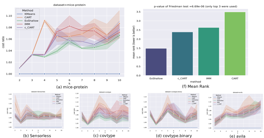
Figure 1: Comparisons over explainable clustering algorithms are shown. (a) shows the comparison for a specific dataset mice-protein. (b), (c), (d) and (e) show comparisons over other datasets - miniaturized to fit the page. (f) shows mean ranks of these techniques over five datasets across model sizes; the Friedman test is conducted over the top three techniques only, with $p=6.688\times{10}^{-6}$.

.

5.1 Algorithms and Hyperparameters

The algorithms we compare and their hyperparameter settings are as follows:

1. Iterative Mistake Minimization (IMM) (Moshkovitz et al. 2020): This generates a decision tree via greedy partitioning using a criterion that minimizes number of mistakes at each split (the number of points separated from their corresponding reference cluster center). There are no parameters to tune. We used the implementation available here: https://github.com/navefr/ExKMC, which internally uses the reference implementation for IMM.

2. ExShallow (Laber, Murtinho, and Oliveira 2021): Here, the decision tree construction explicitly accounts for minimizing explanation complexity while targeting a low cost ratio. The trade-off between clustering cost and explanation size is controlled via a parameter $\lambda$. This is set as $\lambda=0.03$ in our experiments; this value is used in the original paper for various experiments. We used the reference implementation available here: https://github.com/lmurtinho/ShallowTree.

3. CART w/wo COAS: We use CART (Breiman et al. 1984) as the traditional model to compare, and maximize the classification accuracy for predicting clusters, as measured by the F1-macro score. The implementation in scikit (Pedregosa et al. 2011) is used. During training, we set the following parameters: (a) the maximum number of leaves (this represents model size $\eta$ here) is set to the number of clusters $k$, and (b) the parameter class_weight is set to “balanced” for robustness to disparate cluster sizes. Results for CART are denoted with label CART. We then apply COAS to CART; these results are denoted as c_CART. We set $T=2000$, and use default settings for other parameters, e.g., $N_{s}\in[400,|X_{train}|]$. Since we are explaining clusters (and not predicting on unseen data), the training, validation and test sets are identical.

5.2 Experiment Setup

The comparison is performed over five datasets (limited to $1000$ instances), and for each dataset, $k=2,3,...,10$ clusters are produced. Results for the cost ratio (Equation 2) are reported over five trials. Evaluations are performed over the following publicly available datasets: avila, covtype, covtype.binary, Sensorless (Chang and Lin 2011) and mice-protein (Dua and Graff 2017). We specifically picked these datasets since CART is known to perform poorly on them (Frost, Moshkovitz, and Rashtchian 2020; Laber, Murtinho, and Oliveira 2021).

5.3 Observations

Figure 1 presents our results. Figure 1(a) shows the plot for the mice-protein dataset: the $95\%$ confidence interval, in addition to cost ratio, is shown. Plots for other datasets are shown miniaturized - (b), (c), (d), (e) in the interest of space. The cost for k-means is shown for reference a blue horizontal line at $y=1$. Figure 1(f) shows the mean ranks of the various techniques (lower is better) across datasets and number of clusters (as described in Section 4, trials are aggregated over), and its title shows the p-value$=6.688\times 10^{-6}$ of a Friedman test conducted over the top three techniques: we restrict the test to top candidates since otherwise it would be very easy to obtain a low/favorable score, due to the high cost ratios for CART. The low score indicates with high confidence that ExShallow, IMM and c_CART do not produce the same outcomes.

From the plot of mean ranks in Figure 1(f), we observe that although CART performs quite poorly, the application of COAS drastically improves its performance, to the extent that it competes favorably with techniques like IMM and ExShallow; its mean rank places it between them. This is especially surprising given that it doesn’t explicitly minimize the cost in Equation 1. We also note the following p-values from Wilcoxon signed-rank (Wilcoxon 1945) tests:

• CART vs c_CART: $p=1.4783\times 10^{-6}$. The low value indicates that using COAS indeed significantly changes the accuracy of CART.

• IMM vs c_CART: $p=0.0155$. The relatively high value indicates that the performance of c_CART is competitive with IMM.

Here, both the Friedman and Wilcoxon tests are performed for combinations of datasets and $k$ - a “pseudo-dataset”, as discussed in Section 4.

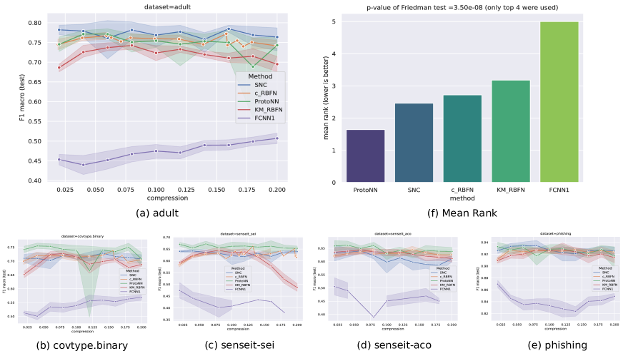
Figure 2: Various prototype-based classifiers are compared. (a) shows comparison for the dataset adult. Number of prototypes are shown as percentage of the training data on the x-axis. (b), (c), (d) and (e) shows plots for other datasets - these are miniaturized to fit the page. (f) shows the mean ranks of techniques based on five datasets; the Friedman test is conducted over the top four techniques only, with $p=3.5025\times 10^{-8}$.

.

6 Protoype-based Classification

Next, we consider prototype-based classification. At training time, such techniques identify “prototypes” (actual training instances or generated instances), that maybe used to classify a test instance based on their similarity to them. A popular technique in this family is the k-Nearest Neighbor (kNN). These are simple to interpret, and if a small but effective set of protoypes maybe identified, they can be convenient to deploy on edge devices (Gupta et al. 2017; Zhang et al. 2020). Prototypes also serve as minimal “look-alike” examples for explaining models (Li et al. 2018; Nauta et al. 2021). Research in this area has focused on minimizing the number of prototypes that need to be retained while minimally trading off accuracy.

We define some notation first. The number of prototypes, which is an input to our experiments, is denoted by $N_{p}$. We will also use $K_{\gamma}(x_{i},x_{j})=e^{-\gamma||x_{i}-x_{j}||_{2}^{2}}$ to denote the Radial Basis Function (RBF) kernel, parameterized by the kernel bandwidth $\gamma$.

6.1 Algorithms and Hyperparameters

These are the algorithms we compare:

1. ProtoNN (Gupta et al. 2017): This technique uses a RBF kernel to aggregate influence of prototypes. Synthetic prototypes are learned and additionally a “score” is learned for each of them that designates their contribution towards each class. The prediction function sums the influence of neighbors using the RBF kernel, weighing contribution towards each class using the learned score values; the class with the highest total score is predicted. The method also allows for reducing dimensionality, but we don’t use this aspect. The various parameters are learned via gradient based optimization.

   We use the EdgeML library (Dennis et al. 2021), which contains the reference implementation for ProtoNN. For optimization, the implementation uses the version of ADAM (Kingma and Ba 2015) implemented in TensorFlow (Abadi et al. 2015); we set $num\_epochs=200$, $learning\_rate=0.05$, while using the defaults for other parameters. The $num\_epochs$ and $learning\_rate$ values are picked based on a limited search among values $\{100,200,300\}$ and $\{0.01,0.05\}$ respectively. The search space explored for $\gamma$ is $[0.001,0.01,0.1,1,10]$. Defaults are used for the other ProtoNN hyperparameters.

2. Stochastic Neighbor Compression (SNC) (Kusner et al. 2014): This also uses a RBF kernel to aggregate influence of prototypes, but unlike ProtoNN, the prediction is performed via the 1-NN rule, i.e., prediction uses only the nearest prototype. The technique bootstraps with randomly sampled $N_{p}$ prototypes (and corresponding labels) from the training data, and then modifies their coordinates for greater accuracy using gradient based optimization; the labels of the prototypes stay unchanged in this process. This is another difference compared to ProtoNN, where in the latter each prototype contributes to all labels to varying extents. The technique maybe extended to reduce the dimensionality of the data (and prototypes); we don’t use this aspect.

   We were unable to locate the reference implementation mentioned in the paper, so we implemented our own version, with the help of the JAXopt library (Blondel et al. 2021). For optimization, gradient descent with backtracking line search is used. A total of $100$ iterations for the gradient search is used (based on a limited search among these values: $\{100,200,300\}$), and each backtracking search is allowed up to $50$ iterations. A grid search over the following values of $\gamma$ is performed: $[0.001,0.01,0.1,1,10]$.

3. Fast Condensed Nearest Neighbor Rule (Angiulli 2005): Learns a “consistent subset” for the training data: a subset such that for any point in the training set (say with label $l$), the closest point in this subset also has a label $l$. Of the multiple variations of this technique proposed in (Angiulli 2005), we use FCNN1, which uses the 1-NN rule for prediction. There are no parameters to tune. We used our own implementation.

   A challenge in benchmarking this technique is it does not accept $N_{p}$ as a parameter; instead it iteratively produces expanding subsets of prototypes until a stopping criteria is met, e.g., if prototype subsets $V_{i}$ and $V_{i+1}$ are produced at iterations $i$ and $i+1$ respectively, then $V_{i}\subset V_{i+1}$. For comparison, we consider the performance at iteration $i$ to be the result of $N_{p}$ prototypes where $N_{p}$ is defined to be $|V_{i}|$.

4. RBFN w/wo COAS: For the traditional model, we use Radial Basis Function Networks (RBFN) (Broomhead and Lowe 1988). For a binary classification problem with classes $\{-1,1\}$, given prototypes $x_{i},i=1,2,...,p$, the label of a test instance $x$ is predicted as $sgn(\sum_{i}^{p}w_{i}K_{\gamma}(x,x_{i}))$ (label $1$ is predicted for a score of $0$). Weights $w_{i}$ are learned using linear regression. A one-vs-rest setup is used for multiclass problems. For our baseline, we use cluster centres of a k-means clustering as our prototypes, where $k$ is set to $N_{p}$. These results are denoted using the term KM_RBFN. In the COAS version, denoted by c_RBFN, the $N_{p}$ prototypes are sampled from the training data. $N_{p}$ represents model size $\eta$ here.

   Note that the standard RBFN, and therefore the variants used here KM_RBFN and c_RBFN, don’t provide a way to reduce dimensionality; this is the reason why this aspect of ProtoNN and SNC wasn’t used (for fair comparison).

   For COAS, we set $T=1000$ and $N_{s}$ was set to $[N_{p}-1,N_{p}]$ to get the desired number of prototypes.

Although all the above techniques use prototypes for classification, it is interesting to note variations in their design: ProtoNN, SNC, KM_RBFN use synthetic prototypes, i.e., they are not part of the training data, while c_RBFN and FCNN1 select $N_{p}$ instances from the training data. The prediction logic also differs: ProtoNN, KM_RBFN, c_RBFN derive a label from some function of the influence by all prototypes, while SNC and FCNN1 use the 1-NN rule.

6.2 Experiment Setup

As before, we evaluate these techniques over five standard datasets: adult, covtype.binary, senseit-sei, senseit-aco, phishing (Chang and Lin 2011). $1000$ training points are used, with $N_{p}\in\{20,40,60,80,100,140,160,180,200\}$. Results are reported over five trials. The score reported is the F1-macro score.

6.3 Observations

Results are shown in Figure 2. (a) shows the plot for the adult dataset. The number of prototypes are shown on the x-axis as percentages of the training data. Plots for other datasets are shown in (b), (c), (d) and (e); these have been miniaturized to fit the page. Figure 2(f) shows the mean rank (lower is better) across datasets and number of prototypes (as described in Section 4, trials are aggregated over). The p-value of the Friedman test is reported, $p=3.5025\times 10^{-8}$. Here too, we do not consider the worst performing candidate, FCNN1 - so as to not bias the Friedman test in our favor.

We observe in Figure 2(f) that while both ProtoNN and SNC outperform c_RBFN, the performance of SNC and c_RBFN are close. We also observe that FCNN1 performs poorly; this matches the observations in Kusner et al. (2014).

We also consider the following p-values from Wilcoxon signed-rank tests:

1. KM_RBFN vs c_RBFN: $p=1.699\times 10^{-4}$. The low value indicates COAS significantly improves upon the baseline KM_RBFN.

2. SNC vs c_RBFN: $p=0.1260$. The relatively high value here indicates that c_RBFN is competitive with SNC; in fact, at a confidence threshold of $0.1$, their outcomes would not be interpreted as significantly different.

As discussed in Section 4, these statistical tests are conducted over a combination of dataset and model size.

7 Random Forest

In the previous sections, we considered the case of scalar model sizes: number of leaves in the case of explanation trees for clustering (Section 5) and number of prototypes in the case of prototype-based classification (Section 6). Here, we assess the effectiveness of the technique when the model size is composed of multiple constraints.

We look at the case of learning Random Forests (RF) where we specify model size using both the number of trees and the maximum depth per tree.

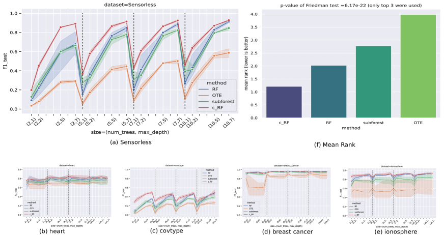
Figure 3: (a) shows results for the dataset=covtype. (b), (c), (d) and (e) show plots for other datasets - miniaturized to fit the page. (f) provides mean ranks, but since there are only two models being compared, the Friedman test cannot be performed.

7.1 Algorithms and Hyperparameters

We compare the standard RF (Breiman 2001) w/wo COAS, with RF pruning techniques such as Optimal Tree Ensembles (OTE) (Khan et al. 2020b) and subforest finding (Zhang and Wang 2009). Both these techniques reduce the number of trees in an RF based on heuristics that depend on factors such as their incremental predictive power and similarity with other trees. In in the interest of space, a detailed description is provided in Section B of the Appendix.

7.2 Experiment Setup

We use the following five standard datasets for this experiment: heart, Sensorless, covtype, ionosphere, breast cancer (Chang and Lin 2011). For each dataset, all size combinations from the following sets are tested (three trials per combination): $num\_trees\in\{2,5,7,10\}$ and
$max\_depth\in\{1,2,5,7\}$. The total dataset size used had $3250$ instances, with $70:30$ split for train to test. For both OTE and the subforest-finding technique, the RFs were originally constructed with $100$ trees, which were then pruned to the desired number. We report the F1-macro score in our experiments.

7.3 Observations

Figure 3(a) shows the results for dataset Sensorless; the x-axis shows values of the tuple $(num\_trees,max\_depth)$ sorted by the first and then the second index. Note the “sawtooth” pattern. For a given value of $num\_trees$, increase in $max\_depth$ leads to increasing accuracy. However, as we move to the next value for $num\_trees$, we start with $max\_depth=1$ again, which leads to a drop in accuracy. This is an artefact of the ordering of the x-axis, and is expected behavior. Plots for other datasets are shown in (b), (c), (d) , (e) - these are miniaturized in the interest of space. Figure 3(f) shows mean ranks across datasets, number of trees and maximum tree depths (across trials).

OTE results are discounted for the Friedman test on account of its relatively poor performance. This gives us a p-value of $p=6.17\times 10^{-22}$, denoting sufficiently different outcomes.

It is easy to see that c_RF is the best performing technique here. The p-value for Wilcoxon signed-rank test wrt the standard RF is $p=1.44\times 10^{-11}$, demonstrating significant improvement.

In the interest of fairness, please note that both OTE and subforest-finding, in their original papers do not restrict the max. depth of trees, and as such, their use here should be seen as a modification, and not indicative of their performance on the original intended use-cases.

8 Discussion and Future Work

The experiments here clearly showcase both the versatility and effectiveness of the strategy of learning the training distribution: it may be applied to different models and notions of model sizes, and can produce results that are competitive to specialized techniques.

Before we conclude, we believe that it is important for us to call out what we are not claiming. We don’t propose that COAS replace the techniques it was compared to without further study, as the latter may offer other task specific benefits, e.g., ExShallow targets certain explanation-quality metrics aside from the cost ratio. Another reason for caution is that the improvements of COAS diminish as model sizes increase (Ghose and Ravindran 2019) ; hence, its utility to a task depends on what model size range is acceptable.

Instead, this work is a humble call to action to explore this strategy - which we believe is relatively unknown today.

In terms of future work, some directions are: (a) learn weights for training instances (as opposed to a distribution) using bilevel optimization (Pedregosa 2016; Franceschi et al. 2018) for the case of a differentiable training loss function, (b) COAS itself may be improved with the use of a different black-box optimizer, and (c) develop a theoretical framework that explains this strategy.

Appendix A Review of COAS

We briefly discuss COAS in this section. Specifically, we discuss the technique from Ghose and Ravindran (2019). We simplify various aspects for brevity - for details please refer to the original paper.

We denote the sampling process used in COAS by $S((X,Y),\Psi,N_{s},p_{o})$. Here, $(X,Y)$ is the data that is to be sampled from (with replacement) and $\Psi,N_{s},p_{o}$ are parameters used for sampling. These are defined as follows:

• $\Psi$: This is a probability density function (pdf) defined over the data $(X,Y)$ and denotes the sampling probability of instances.

• $N_{s}$: Sample size.

• $p_{o}$: The fraction of samples that are to be sampled uniformly randomly from $(X,Y)$. The remaining $(1-p_{o})N_{s}$ samples are chosen with replacement from $(X,Y)$ based on the probabilities $p((X,Y);\Psi)$.

$p_{o}$ serves as a “shortcut” for the model to combine data that was provided with data from the learned distribution. Since the train and test data splits provided are assumed to come from the same distribution, $p_{o}$ also acts as tool for analyzing the “mix” of data preferred at various model sizes. For example, an interesting result shown (Ghose and Ravindran 2019) is that as model size increases, $p_{o}\rightarrow 1$, i.e., the best training distribution at large sizes is the test distribution, which is the commonly known case.

To state the optimize problem COAS solves, we introduce additional notation:

1. Let $(X_{train},Y_{train})$ and $(X_{val},Y_{val})$ represent training and validation datasets respectively.

2. Let $train_{\mathcal{F}}(\eta,(X,Y))$ be a training algorithm that returns a model of size $\eta$ from model family $\mathcal{F}$ when supplied with training data $(X,Y)$.

3. Let $acc(f,(X,Y))$ denote the accuracy of model $f$ on dataset $(X,Y)$.

Then, COAS performs the following optimization for user-specified $\eta$ over $T$ iterations:

$$\max_{\Psi,N_{s},p_{o}}\;acc(f,(X_{val},Y_{val}))$$ (3)

where, $$f=train_{\mathcal{F}}(\eta,(X_{sample},Y_{sample})$$ (4)

and $$(X_{sample},Y_{sample})=S((X_{train},y_{train}),\Psi,N_{s},p_{o})$$ (5)

Essentially, COAS identifies parameters $\Psi,N_{s},p_{o}$ such that a model trained on data sampled using them, maximizes validation accuracy. Note that since $S()$ samples with replacement, it is possible to have an optimal $N_{s}$ that’s larger thann the size of the training data. A Bayesian Optimizer is used for optimization, and a budget of $T$ iterations is provided. There is no other stopping criteria, i.e., the optimizer is run all the way through $T$ iterations.

Appendix B Random Forest Comparison Algorithms

We describe in detail the algorithms that were compared for RF-based classification. These were briefly mentioned in Section 7.1.

1. Optimal Tree Ensembles (OTE) (Khan et al. 2020b): This is a technique to prune a RF to produce a lower number of trees. The pruning occurs in two phases: (a) first, the top $M$ trees are retained based on prediction accuracy on out-of-bag examples, and (b) further pruning is performed based on a tree’s contribution to the overall Brier score on a validation set. In our experiments, $M$ was set to $20\%$ of the initial number of trees in the forest.

   Although a reference R package exists (Khan et al. 2020a), it doesn’t allow to set the max. depth of trees, which is relevant here. Hence we use our implementation.

2. Finding a subforest (Zhang and Wang 2009): This paper proposes multiple techniques to prune the number of trees in an RF. Among them it shows that pruning based on incremental predictive power of trees performs best. Hence, this is the technique we use here, based on our own implementation.

3. RF w/wo COAS: We train standard RFs (Breiman 2001) without and with COAS, denoted as RF and c_RF respectively. For COAS, we set number of iterations as $T=3000$ and $N_{s}\in[30,|X_{train}|]$ (the lower bound was obtained by limited search). The implementation in scikit is used, and for standard RF models, i.e., without COAS, the parameter class_weight is set to “balanced_subsample” to make them robust to class imbalance.

References

- Abadi et al. (2015) Abadi, M.; Agarwal, A.; Barham, P.; Brevdo, E.; Chen, Z.; Citro, C.; Corrado, G. S.; Davis, A.; Dean, J.; Devin, M.; Ghemawat, S.; Goodfellow, I.; Harp, A.; Irving, G.; Isard, M.; Jia, Y.; Jozefowicz, R.; Kaiser, L.; Kudlur, M.; Levenberg, J.; Mané, D.; Monga, R.; Moore, S.; Murray, D.; Olah, C.; Schuster, M.; Shlens, J.; Steiner, B.; Sutskever, I.; Talwar, K.; Tucker, P.; Vanhoucke, V.; Vasudevan, V.; Viégas, F.; Vinyals, O.; Warden, P.; Wattenberg, M.; Wicke, M.; Yu, Y.; and Zheng, X. 2015. TensorFlow: Large-Scale Machine Learning on Heterogeneous Systems. Software available from tensorflow.org.
- Angiulli (2005) Angiulli, F. 2005. Fast Condensed Nearest Neighbor Rule. In Proceedings of the 22nd International Conference on Machine Learning, ICML ’05, 25–32. New York, NY, USA: Association for Computing Machinery. ISBN 1595931805.
- Benavoli, Corani, and Mangili (2016) Benavoli, A.; Corani, G.; and Mangili, F. 2016. Should We Really Use Post-Hoc Tests Based on Mean-Ranks? Journal of Machine Learning Research, 17(5): 1–10.
- Blondel et al. (2021) Blondel, M.; Berthet, Q.; Cuturi, M.; Frostig, R.; Hoyer, S.; Llinares-López, F.; Pedregosa, F.; and Vert, J.-P. 2021. Efficient and Modular Implicit Differentiation. arXiv preprint arXiv:2105.15183.
- Breiman (2001) Breiman, L. 2001. Random Forests. Machine Learning, 45(1): 5–32.
- Breiman et al. (1984) Breiman, L.; et al. 1984. Classification and Regression Trees. New York: Chapman & Hall. ISBN 0-412-04841-8.
- Broomhead and Lowe (1988) Broomhead, D.; and Lowe, D. 1988. Multivariable Functional Interpolation and Adaptive Networks. Complex Systems, 2: 321–355.
- Chang and Lin (2011) Chang, C.-C.; and Lin, C.-J. 2011. LIBSVM: A library for support vector machines. ACM Transactions on Intelligent Systems and Technology, 2: 27:1–27:27. Software available at http://www.csie.ntu.edu.tw/~cjlin/libsvm, datasets at https://www.csie.ntu.edu.tw/~cjlin/libsvmtools/datasets/.
- Demšar (2006) Demšar, J. 2006. Statistical Comparisons of Classifiers over Multiple Data Sets. Journal of Machine Learning Research, 7(1): 1–30.
- Dennis et al. (2021) Dennis, D. K.; Gaurkar, Y.; Gopinath, S.; Goyal, S.; Gupta, C.; Jain, M.; Jaiswal, S.; Kumar, A.; Kusupati, A.; Lovett, C.; Patil, S. G.; Saha, O.; and Simhadri, H. V. 2021. EdgeML: Machine Learning for resource-constrained edge devices.
- Dua and Graff (2017) Dua, D.; and Graff, C. 2017. UCI Machine Learning Repository.
- Feldman (2000) Feldman, J. 2000. Minimization of Boolean complexity in human concept learning. Nature, 407: 630–3.
- Franceschi et al. (2018) Franceschi, L.; Frasconi, P.; Salzo, S.; Grazzi, R.; and Pontil, M. 2018. Bilevel Programming for Hyperparameter Optimization and Meta-Learning. In Dy, J.; and Krause, A., eds., Proceedings of the 35th International Conference on Machine Learning, volume 80 of Proceedings of Machine Learning Research, 1568–1577. PMLR.
- Frost, Moshkovitz, and Rashtchian (2020) Frost, N.; Moshkovitz, M.; and Rashtchian, C. 2020. ExKMC: Expanding Explainable -Means Clustering. arXiv preprint arXiv:2006.02399.
- Ghose (2020) Ghose, A. 2020. compactem. Software available at https://compactem.readthedocs.io/en/latest/index.html.
- Ghose and Ravindran (2019) Ghose, A.; and Ravindran, B. 2019. Learning Interpretable Models Using an Oracle. CoRR, abs/1906.06852.
- Ghose and Ravindran (2020) Ghose, A.; and Ravindran, B. 2020. Interpretability With Accurate Small Models. Frontiers in Artificial Intelligence, 3.
- Gupta et al. (2017) Gupta, C.; Suggala, A. S.; Goyal, A.; Simhadri, H. V.; Paranjape, B.; Kumar, A.; Goyal, S.; Udupa, R.; Varma, M.; and Jain, P. 2017. ProtoNN: Compressed and Accurate kNN for Resource-scarce Devices. In Precup, D.; and Teh, Y. W., eds., Proceedings of the 34th International Conference on Machine Learning, volume 70 of Proceedings of Machine Learning Research, 1331–1340. PMLR.
- Japkowicz and Shah (2011) Japkowicz, N.; and Shah, M. 2011. Evaluating Learning Algorithms: A Classification Perspective. Cambridge University Press.
- Khan et al. (2020a) Khan, Z.; Gul, A.; Perperoglou, A.; Mahmoud, O.; Adler, W.; Miftahuddin; and Lausen, B. 2020a. compactem. Software available at https://cran.r-project.org/web/packages/OTE/.
- Khan et al. (2020b) Khan, Z.; Gul, A.; Perperoglou, A.; Miftahuddin, M.; Mahmoud, O.; Adler, W.; and Lausen, B. 2020b. Ensemble of optimal trees, random forest and random projection ensemble classification. Advances in Data Analysis and Classification, 14(1): 97–116.
- Kingma and Ba (2015) Kingma, D. P.; and Ba, J. 2015. Adam: A Method for Stochastic Optimization. In Bengio, Y.; and LeCun, Y., eds., 3rd International Conference on Learning Representations, ICLR 2015, San Diego, CA, USA, May 7-9, 2015, Conference Track Proceedings.
- Kusner et al. (2014) Kusner, M.; Tyree, S.; Weinberger, K.; and Agrawal, K. 2014. Stochastic Neighbor Compression. In Xing, E. P.; and Jebara, T., eds., Proceedings of the 31st International Conference on Machine Learning, volume 32 of Proceedings of Machine Learning Research, 622–630. Bejing, China: PMLR.
- Laber, Murtinho, and Oliveira (2021) Laber, E. S.; Murtinho, L.; and Oliveira, F. 2021. Shallow decision trees for explainable k-means clustering. CoRR, abs/2112.14718.
- Lage et al. (2019) Lage, I.; Chen, E.; He, J.; Narayanan, M.; Kim, B.; Gershman, S. J.; and Doshi-Velez, F. 2019. Human Evaluation of Models Built for Interpretability. Proceedings of the AAAI Conference on Human Computation and Crowdsourcing, 7(1): 59–67.
- Li et al. (2018) Li, O.; Liu, H.; Chen, C.; and Rudin, C. 2018. Deep Learning for Case-Based Reasoning through Prototypes: A Neural Network That Explains Its Predictions. In Proceedings of the Thirty-Second AAAI Conference on Artificial Intelligence and Thirtieth Innovative Applications of Artificial Intelligence Conference and Eighth AAAI Symposium on Educational Advances in Artificial Intelligence, AAAI’18/IAAI’18/EAAI’18. AAAI Press. ISBN 978-1-57735-800-8.
- Makarychev and Shan (2022) Makarychev, K.; and Shan, L. 2022. Explainable K-Means: Don’t Be Greedy, Plant Bigger Trees! In Proceedings of the 54th Annual ACM SIGACT Symposium on Theory of Computing, STOC 2022, 1629–1642. New York, NY, USA: Association for Computing Machinery. ISBN 9781450392648.
- Moshkovitz et al. (2020) Moshkovitz, M.; Dasgupta, S.; Rashtchian, C.; and Frost, N. 2020. Explainable k-Means and k-Medians Clustering. In III, H. D.; and Singh, A., eds., Proceedings of the 37th International Conference on Machine Learning, volume 119 of Proceedings of Machine Learning Research, 7055–7065. PMLR.
- Murshed et al. (2021) Murshed, M. G. S.; Murphy, C.; Hou, D.; Khan, N.; Ananthanarayanan, G.; and Hussain, F. 2021. Machine Learning at the Network Edge: A Survey. ACM Comput. Surv., 54(8).
- Nauta et al. (2021) Nauta, M.; Jutte, A.; Provoost, J.; and Seifert, C. 2021. This Looks Like That, Because … Explaining Prototypes for Interpretable Image Recognition. In Kamp, M.; Koprinska, I.; Bibal, A.; Bouadi, T.; Frénay, B.; Galárraga, L.; Oramas, J.; Adilova, L.; Krishnamurthy, Y.; Kang, B.; Largeron, C.; Lijffijt, J.; Viard, T.; Welke, P.; Ruocco, M.; Aune, E.; Gallicchio, C.; Schiele, G.; Pernkopf, F.; Blott, M.; Fröning, H.; Schindler, G.; Guidotti, R.; Monreale, A.; Rinzivillo, S.; Biecek, P.; Ntoutsi, E.; Pechenizkiy, M.; Rosenhahn, B.; Buckley, C.; Cialfi, D.; Lanillos, P.; Ramstead, M.; Verbelen, T.; Ferreira, P. M.; Andresini, G.; Malerba, D.; Medeiros, I.; Fournier-Viger, P.; Nawaz, M. S.; Ventura, S.; Sun, M.; Zhou, M.; Bitetta, V.; Bordino, I.; Ferretti, A.; Gullo, F.; Ponti, G.; Severini, L.; Ribeiro, R.; Gama, J.; Gavaldà, R.; Cooper, L.; Ghazaleh, N.; Richiardi, J.; Roqueiro, D.; Saldana Miranda, D.; Sechidis, K.; and Graça, G., eds., Machine Learning and Principles and Practice of Knowledge Discovery in Databases, 441–456. Cham: Springer International Publishing. ISBN 978-3-030-93736-2.
- Pedregosa (2016) Pedregosa, F. 2016. Hyperparameter Optimization with Approximate Gradient. In Proceedings of the 33rd International Conference on International Conference on Machine Learning - Volume 48, ICML’16, 737–746. JMLR.org.
- Pedregosa et al. (2011) Pedregosa, F.; Varoquaux, G.; Gramfort, A.; Michel, V.; Thirion, B.; Grisel, O.; Blondel, M.; Prettenhofer, P.; Weiss, R.; Dubourg, V.; Vanderplas, J.; Passos, A.; Cournapeau, D.; Brucher, M.; Perrot, M.; and Duchesnay, E. 2011. Scikit-learn: Machine Learning in Python. Journal of Machine Learning Research, 12: 2825–2830.
- Poursabzi-Sangdeh et al. (2021) Poursabzi-Sangdeh, F.; Goldstein, D.; Hofman, J.; Wortman Vaughan, J.; and Wallach, H. 2021. Manipulating and Measuring Model Interpretability. In CHI 2021.
- Ribeiro, Singh, and Guestrin (2016) Ribeiro, M. T.; Singh, S.; and Guestrin, C. 2016. “Why Should I Trust You?”: Explaining the Predictions of Any Classifier. In Proceedings of the 22Nd ACM SIGKDD International Conference on Knowledge Discovery and Data Mining, KDD ’16, 1135–1144. New York, NY, USA: ACM. ISBN 978-1-4503-4232-2.
- Sanchez-Iborra and Skarmeta (2020) Sanchez-Iborra, R.; and Skarmeta, A. F. 2020. TinyML-Enabled Frugal Smart Objects: Challenges and Opportunities. IEEE Circuits and Systems Magazine, 20(3): 4–18.
- Shahriari et al. (2016) Shahriari, B.; Swersky, K.; Wang, Z.; Adams, R.; and De Freitas, N. 2016. Taking the human out of the loop: A review of Bayesian optimization. Proceedings of the IEEE, 104(1): 148–175. Publisher Copyright: © 1963-2012 IEEE.
- Wilcoxon (1945) Wilcoxon, F. 1945. Individual Comparisons by Ranking Methods. Biometrics Bulletin, 1(6): 80–83.
- Zhang and Wang (2009) Zhang, H.; and Wang, M. 2009. Search for the smallest random forest. Statistics and its interface, 2: 381.
- Zhang et al. (2020) Zhang, W.; Chen, X.; Liu, Y.; and Xi, Q. 2020. A Distributed Storage and Computation k-Nearest Neighbor Algorithm Based Cloud-Edge Computing for Cyber-Physical-Social Systems. IEEE Access, 8: 50118–50130.