Finding and Exploring Promising Search Space for the 0-1 Multidimensional Knapsack Problem

Abstract

The 0-1 Multidimensional Knapsack Problem (MKP) is a classical NP-hard combinatorial optimization problem with many engineering applications. In this paper, we propose a novel algorithm combining evolutionary computation with exact algorithm to solve the 0-1 MKP. It maintains a set of solutions and utilizes the information from the population to extract good partial assignments. To find high-quality solutions, an exact algorithm is applied to explore the promising search space specified by the good partial assignments. The new solutions are used to update the population. Thus, the good partial assignments evolve towards a better direction with the improvement of the population. Extensive experimentation with commonly used benchmark sets shows that our algorithm outperforms the state of the art heuristic algorithms, TPTEA and DQPSO. It finds better solutions than the existing algorithms and provides new lower bounds for 8 large and hard instances.

1 Introduction

The 0-1 Multidimensional Knapsack Problem (MKP) is a well-known combinatorial optimization problem that has been applied in different practical domains. Given a set $N$ = {1, 2, …, $n$} of items with profits $p_{i}>0$ and a set $M$ = {1, 2, …, $m$} of resources with a capacity $b_{j}>0$ for each resource. Each item $i$ consumes a given amount of each resource $r_{ij}>0$. The 0-1 MKP is to select a subset of items that maximizing the sum of the profits without exceeding the capacity of each resource. The problem is formally stated as:

$$\text{Maximize }\ f=\sum^{n}_{i=1}p_{i}x_{i}$$

$$\text{s.t. }\sum^{n}_{i=1}r_{ij}x_{i}\leq b_{j},j\in M=\{1,2,...,m\}$$

$$x_{i}\in\{0,1\},i\in N=\{1,2,...,n\}$$

where each $x_{i}$ is a binary variable indicating whether the item $i$ is selected, i.e., $x_{i}$ = 1 if the item is selected, and 0 otherwise.

The 0-1 MKP has many real-world engineering applications, such as resource allocation [1], cutting stock [2], portfolio-selection [3], obnoxious facility location[4], etc. Due to its NP-hard characteristic, solving the MKP is computationally challenging. The exact algorithms for MKP are usually based on branch and bound algorithms, such as the CORAL algorithm [5]. However, the modern exact algorithms could solve only the MKP instances of relatively small and moderate size, i.e., the instances with less than 250 items and less than 10 resource constraints. For larger instances with more than 500 items and more than 30 resource constraints, the heuristic algorithms are usually better choices. There exist a number of heuristic algorithms for the problem. For instance, the single-solution based local search algorithms maintain a solution during search and iteratively optimize the solution during search. The representative of these algorithms include tabu search[6], simulated annealing [7] and kernel search[8]. The population-based evolutionary algorithms are also popular for the problem, such as hybrid binary particle swarm optimization[9, 10, 11, 12], ant colony optimization[13, 14], moth search optimization[15], Pigeon Inspired Optimization[16, 17], bee colony algorithm[18], quantum cuckoo search algorithm[19], fruit fly optimization algorithm[20, 21] and grey wolf optimizer[22]. Recently, machine learning assisted methods[23, 24, 25], along with probability learning-based algorithms[26] emerged. However, heuristics algorithms are still popular choice when solving some large and hard MKP instances in practical. To our best knowledge, the TPTEA algorithm [27] provided the last updates of the lower bounds of the commonly used benchmark set containing the large instances with 500 items and 30 resource constraints. Compared with TPTEA, the DQPSO [10] algorithm loses a little in the final solution quality, but it finds high-quality solutions earlier than TPTEA.

In this paper, we propose a novel algorithm for solving the 0-1 Multidimensional Knapsack Problem. The algorithm finds promising partial assignments by an adapted evolutionary algorithm and explores the promising search space specified by the partial assignments with an exact algorithm. It utilizes the advantages of Evolutionary Computation and Large Neighbourhood Search (LNS) [28] in its major components. Consequently, it performs well when solving some large and hard 0-1 MKP benchmark instances. Our experiments run with 281 commonly used benchmark instances show that our algorithm performs better than the state of the art heuristic algorithms including TPTEA and DQPSO. Our contribution can be summarized as, (1) We propose to combine Evolutionary Computation with exact algorithm to solve the 0-1 MKP. (2) We adopt and adapt the TPTEA algorithm to find promising partial assignments from the population. (3) Our algorithm provides new lower bound for 8 hard and large instances.

The paper is organized as follows. We first introduce the motivation and the raw idea of our algorithm in Section 2. The details of the proposed algorithm, including the framework of the new algorithm, the adaption of the TPTEA algorithm for finding good partial assignments, a customized LNS, are present in Section 3. The experimental results are shown in Section 4. We discussed our algorithm with some closely related methods in Section 5. Finally, Section 6 is the conclusion.

2 The Motivation and The Main Idea

An assignment $\mathcal{A}$ to items $I\subseteq N$ is a set of instantiations of the form ($x_{i}=v_{i}$), one for each $i\in N$ to assign $v_{i}$ to $x_{i}$ where $v_{i}\in\{0,1\}$. If $I=N$, then $\mathcal{A}$ is a complete assignment; otherwise a partial assignment. A complete assignment $s$ that satisfies all resource constraints is a feasible solutions to the instance, or a solution for short. A solution $s$ is an optimal solution if its objective value $f(s)$ is larger than or equal to that of any other solution to the instance. A partial assignment is an optimal one if it can be extended to an optimal solution.

Given an MKP instance $P$ with $n$ items, the size of the search space of finding an optimal solution for $P$ is $2^{n}$. Given a partial assignment $\mathcal{A}$ of $P$. Fixing the values of $\mathcal{A}$ in $P$ will result in a sub-problem $P^{\prime}$ whose search space is $2^{n-|\mathcal{A}|}$. The search space of $P^{\prime}$ can be considered as a sub search space of $P$ which is specified by $\mathcal{A}$. If we are given an optimal partial assignment $\mathcal{A^{*}}$ of $P$, then we can find an optimal solution for $P$ in a search space of size $2^{n-|\mathcal{A^{*}}|}$ instead of the entire search space of size $2^{n}$. However, as far as we know, there is no existing method that identifies optimal partial assignment for general 0-1 MKP before solving it exactly. Thus, the aim of our algorithm is to find good partial assignments that have a large possibility of being an optimal one, or can be extended to a high-quality solution whose objective value is close to that of an optimal solution. Then exploring the promising search space specified by the good partial assignments may find high-quality solutions efficiently.

Evolutionary Algorithms (EA) are powerful techniques for solving combinatorial optimization problems based on the simulation of biological evolution. They start from a population of individuals (representing solutions) and produces offspring (new solutions) by utilizing the information of the population. Guided by a fitness function measuring the quality of a solution, the new solutions with high-quality are usually used to update the population. As a result, the population evolves towards the direction of better fitness function. One of the advantages of EA is to identify and keep some high-quality patterns (partial assignments) in the population, so they can produce high-quality solutions through crossover and mutation operations. Thus, we propose a novel algorithm that combines Evolutionary Algorithm with exact algorithm for the 0-1 MKP. The main idea of the algorithm is shown in Algorithm 1.

Input: a MKP instance $P$;

Output: current best solution $s^{*}$;

1

2$population\leftarrow$ initPopulation($P$);

3 $s^{*}\leftarrow$ the best solution in $population$;

4 while the termination condition is not reached do

5       $pa\leftarrow extract(population)$;

6       $s\leftarrow explore(P,pa)$;

7       updatePopulation($s$);

8       if $f(s)>f(s^{*})$ then

9             $s^{*}\leftarrow s$;

10            

11      

12return $s^{*}$;

Algorithm 1 The main idea

At the beginning, the population of Evolutionary Algorithm, a set of solutions recorded in $population$ is initialized at line 1. The $s^{*}$ records the best solution found so far. The loop at lines 3-8 is the main procedure, e.g., a promising partial assignment pa is extracted from the population by an Evolutionary Algorithm at line 4 and the promising search space is explored by an exact algorithm at line 5. The new solution is used to update the population at line 6. If a better solution is found, $s^{*}$ will be updated accordingly at lines 7-8, The procedure repeats until a termination condition is reached and the best found solution is returned. There are various termination conditions that can be used in the algorithm, such as a time limit or the number of iterations.

3 Combining Evolutionary Algorithm with Integer Programming for MKP

Based on the idea proposed in last section, we introduce the detailed algorithm for solving the 0-1 MKP, namely finding and exploring promising search space (FEPSS). The framework of the algorithm is presented first.

3.1 The Framework

The main procedure of FEPSS is present in Algorithm 2. At the beginning, the population, a set of solutions, is initialized at line 1 and the current best solution is initialized to the best one of the initial population. There are two cases to find and explore good partial assignments. In the first case (lines 10-12), the good partial assignments are extracted from the population at line 12 and the search space specified by $pa$ is explored at line 13. In the second case (lines 6-8), we run a customized Large Neighbourhood Search procedure to refine current best solution. Each of the two cases returns a new solution $s$, which is used to update the population at line 13 and update the current best solution at line4 14-16. A counter num is used to record the number of the first case is executed. If the counter reaches a predefined parameter lnsLimit or the best solution is updated, the second case will be executed once. The details of the procedures called in the framework will be introduced in the following subsections.

Input: a MKP instance $P$;

Output: current best solution $s^{*}$;

1

2$population\leftarrow$ initPopulation($P$);

3 $s^{*}\leftarrow$ the best solution in $population$;

4 $num\leftarrow 0$;

5 while the termination condition is not reached do

6       if iterationNum = lnsLimit or bestUpdated then

7             $bestUpdated\leftarrow false$;

8             $num\leftarrow 0$;

9             $s\leftarrow$ LNS($P$, $s^{*}$);

10            

11      else

12             $num\leftarrow num+1$;

13             $pa\leftarrow$ extractFromPopulation($P$);

14             $s\leftarrow$ explore($P$, $pa$);

15            

16      updatePopulation($s$);

17       if  $f(s)>f(s^{*})$ then

18             $bestUpdated\leftarrow true$;

19             $s^{*}\leftarrow s$;

20            

21      

22return $s^{*}$;

Algorithm 2 The framework

Note that there is a preprocessing step ahead of the algorithm, e.g., all the items are preprocessed and renumbered in an ascending order of a coarse-grained evaluation of the items, which is defined as follows.

$$c_{i}=\frac{p_{i}}{\sum^{m}_{j=1}\frac{r_{ij}}{b_{j}}},\forall i\in\{1,2,...,n\}$$ (1)

After the items are renumbered, the corresponding $p_{i}$ and $r_{ij}$ are adjusted accordingly. In the following, all the items will be used with their new numbering. An item $i$ is selected (not selected) in a solution means that the value of the corresponding variable $x_{i}$ is 1 (0), and vice versa. $population[k]$ is the $k$-$th$ solution in $population$ and $s[i]$ is the value of variable $x_{i}$ in solution $s$.

In the following subsections, we will introduce the initPopulation, extractFromPopulation, LNS, explore and updatePopulation procedures in details.

3.2 Initializing the Population

The solution set $population$ contains $ns$ solutions. At the beginning, we randomly generate $ns\times 1000$ solutions and add the best $ns$ ones into $population$ (selected by their objectives). Then we run a tabu search to refine the random solutions in $population$. The procedure of generating initial $population$ is present in Algorithm 3.

When generating a random solution, the geneRandomSolutions procedure randomly selects an item and tries to add it into the knapsack. The item is added into the knapsack if no resource constraint is violated; otherwise, it is skipped. A random solution will be generated after all items are tried.

To refine the random solutions, the tabu search strategy of the first phase of TPTEA algorithm is employed [27]. We briefly recall the procedure here. It explores only the feasible search space and uses two basic neighborhoods: the one-flip neighborhood $N_{1}(s)$ and the swap neighborhood $N_{2}(s)$. The $N_{1}(s)$ contains all the feasible solutions which can be obtained by applying the $flip$ operator that changes the value of the variable $x_{q}$ in $s$ to its complementary value 1 - $x_{q}$. The $N_{2}(s)$ contains all the feasible solutions which can be obtained by applying the $swap$ operator that swaps the values of two variables with different values in $s$. The tabuSearch procedure is shown in Algorithm 4. It always finds the best neighbour from current neighbourhood $N_{1}(s)\bigcup N_{2}(s)$ and mains a record of all the visited solutions to avoid duplicate visiting. The tabu function is implemented with three hashing vectors [29]. The best solution visited during the tabu search is returned.

Input: a MKP instance $P$;

Output: a solution set $population$;

1 $population\leftarrow$ geneRandomSolutions();

2 for $i=1$ to $ns$ do

3       $population[i]\leftarrow$ tabuSearch($population[i]$);

4      

5return $population$;

Algorithm 3 initPopulation

Input: a solution $s$;

Output: a refined solution $s^{\prime}$;

1 $iteration\leftarrow 1$;

2 $tabuList\leftarrow\emptyset$;

3 $s^{\prime}\leftarrow s$;

4 while $iteration\leq maxIteration$ do

5       find a best neighbor solution $s_{neighbor}$ from $N_{1}(s)\bigcup N_{2}(s)$, which is not in $tabuList$;

6       $s\leftarrow s_{neighbor}$;

7       if $f(s)>f(s^{\prime})$ then

8             $s^{\prime}\leftarrow s$;

9            

10      add $s$ into $tabuList$;

11       $iteration\leftarrow iteration+1$;

12      

13

14return $s^{\prime}$;

Algorithm 4 tabuSearch

3.3 Extracting High-quality Partial Assignments from The Population

In this subsection, we introduce how to extract good partial assignments from the population. The idea is to divide the items into two parts: the fixed part and the free part. Then we generate a partial assignment for the fixed part and explore the free part with an exact algorithm. The extractFromPopulation procedure is shown in Algorithm 5. It decides items in the fixed part at lines 1-8 and then assigns values to the items in the fixed part at lines 13-25 to generate a partial assignment. The details of the algorithm are as follows.

Input: a MKP instance $P$;

Output: a partial assignment $pa$;

1 calculate $\delta_{i}$ for each item $i$;

2 $t\leftarrow$ number of items selected in $s^{*}$;

3 sort all items by the ascending order of $\delta_{i}$;

4 $fix\leftarrow\emptyset$;

5 for each $i\in[1,n-t-\Delta)$ do

6       $fix\leftarrow fix\cup\{i\}$;

7      

8for each $i\in(n-t+\Delta,n]$ do

9       $fix\leftarrow fix\cup\{i\}$;

10      

11

12$num\leftarrow\frac{ns}{10}$;

13 $pa\leftarrow\emptyset$;

14 $exceed\leftarrow true$;

15 while $exceed$ do

16      

17      for  each $i\in fix$ do

18             $selectedNum\leftarrow 0$;

19             for $j=1$ to $num$ do

20                   $s\leftarrow$ select a solution from $population$ randomly;

21                   if s$[i]=1$ then

22                         $selectedNum\leftarrow selectedNum+1$;

23                        

24                  

25            $v\leftarrow 1$;

26             if $selectedNum<\frac{num}{2}$ then

27                   $v\leftarrow 0$;

28                  

29            $r\leftarrow rand(0,1)$;

30             if $r<\frac{1}{n\times 10}$ then

31                   $v\leftarrow 1-v$;

32                  

33            $pa\leftarrow pa\cup(x_{i},v)$;

34            

35      if the items selected in $pa$ violate no resource constraint then

36             $exceed\leftarrow false$;

37            

38      else

39             $pa\leftarrow\emptyset$;

40            

41      

42

43return $pa$;

Algorithm 5 extractFromPopulation

Firstly, each item $i$ is associated with a score $\delta_{i}$ defined as:

$$\delta_{i}=\beta\times\frac{w_{i}}{ns}+(1-\beta)\times\frac{\frac{i}{n}+rand(0,1)}{2}$$ (2)

where $\beta\in(0,1)$ is a parameter, $rand(0,1)$ returns a random number in (0, 1) and $w_{i}$ is defined as:

$$w_{i}=\sum^{ns}_{k=1}population[k][i]$$ (3)

Thus, $\frac{w_{i}}{ns}$ indicates the proportion of solutions in $population$ selecting item $i$. The items are renumbered by the score defined in formula (1), so $\frac{i}{n}$ indicates how likely item $i$ is selected by the coarse-grained evaluation. We would prefer adding the items with higher $\delta_{i}$ into the knapsack.

Secondly, we count the number of items selected in current best solution $s^{*}$, i.e., $t=\sum^{n}_{i=1}s^{*}[i]$. Then we sort the items in ascending order of $\delta_{i}$. The items $i\in[1,n-t-\Delta)$ and the items $i\in(n-t+\Delta,n]$ compose a fixed part which is recorded in $fix$ at lines 4-8, and the remaining items $i\in[n-t-\Delta,n-t+\Delta]$ compose a free part, where $\Delta$ is a parameter. We make such selections because the items with smaller $\delta_{i}$ have larger possibility of not being selected and the ones with larger $\delta_{i}$ have larger possibility of being selected, and the free part should contain those hard to decide items. The strategy eliminates the items locating near the head (items with small $\delta_{i}$) and the end (items with large $\delta_{i}$) of the ordering. As is shown in Figure 1, the blue ones are fixed part and the red ones are free part.

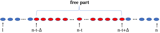
Figure 1: Example of fixed part and free part.

Although the score $\delta_{i}$ gives a recommendation to the values of variables in the fixed part, we design a more elaborate strategy to determine the values to avoid local optimum (lines 14-21 in Algorithm 5). For each item in the fixed part, we randomly select $\frac{ns}{10}$ solutions from the solution set $population$. Then we count the number of the selected solutions containing the item, recorded in $selectedNum$ (lines 15-18). An item is selected if more than half of the $\frac{ns}{10}$ solutions contain the item (lines 19-21). A mutation operation that flips the value with probability $\frac{1}{n\times 10}$ is used at lines 22 to 24. The while loop at line 12 and the if condition at line 26 ensure that the generated partial assignment violates no resource constraint. After the partial assignment $pa$ is generated, an exact algorithm (Integer Programming) is employed to explore the corresponding search space, which will be introduced later.

3.4 The Customized Large Neighbourhood Search

In this subsection, we introduce a customized Large Neighbourhood Search procedure to refine current best solution. The procedure of extracts good partial assignments from current best solution and explores the sub-space specified by the partial assignments to find high-quality solutions. It also uses the information of the population to select some items that compose a free part and the remaining items compose the fixed part. We keep the values in current best solution for the fixed part to generate a partial assignment. The LNS procedure is shown in Algorithm 6.

Input: a MKP $P$ and current best solution $s^{*}$

Output: a solution $s$;

1 $s\leftarrow null$;

2 for $i=1$ to $lnsIterationNum$ do

3       $var_{1}\leftarrow$ votingFunction();

4       $var_{2}\leftarrow$ randomFunction();

5       $var_{3}\leftarrow$ ratioFunction();

6       $free\leftarrow var_{1}\cup var_{2}\cup var_{3}$;

7       $pa\leftarrow s^{*}-free$;

8       $s^{\prime}\leftarrow$ explore($P$, $pa$);

9       updatePopulation($s^{\prime}$);

10       if $s=null$ or $f(s^{\prime})>f(s)$ then

11             $s\leftarrow s^{\prime}$;

12            

13      

14return $s$;

Algorithm 6 LNS

We propose three functions, votingFunction, randomFunction and ratioFunction to select the items belonging to the free part. Each of them will find a set of items and their union constitutes the free part (lines 3-7). Then we remove the assignments of the free part from current best solution $s^{*}$, and the remaining constitute a partial assignment $pa$ (line 7).

The votingFunction is based on the score $w_{i}$ defined in formula (3) which records the number of solutions in $population$ voting for the selection of the item. The function selects items into free part in two cases: (1) item $i$ is in $s^{*}$ and $w_{i}<ns-\sigma$; (2) item $i$ is not in $s^{*}$ and $w_{i}>\sigma$, where $\sigma$ is the standard deviation of $W=\{w_{1},w_{2},...,w_{n}\}$.

The following two functions work on the renumbered items which are sorted by the ascending order of formula (1). The randomFunction simply selects each item indexed from $index_{1}$ to $n$ with probability $P_{1}$, where $index_{1}$ points to the first item with $w_{i}\geq\frac{ns}{2}$.

The ratioFunction uses another index $index_{2}$ that points to the first item with $w_{i}\geq 1$. It makes selections in the items indexed from $index_{2}$ to $index_{1}$ only. For each item $i$, we calculates its average profit $\frac{p_{i}}{r_{ij}}$ in each resource constraint $j$. In each resource constraint, we can find a set of items containing the top $t_{2}$ items with the largest average profit in this constraint. If an item has appeared in any of the sets, it will be selected with a probability $P_{2}$.

The LNS procedure calls the three functions to select the items belonging to the free part at lines 3-5. After that, it combines the three item sets to get the free part at line 6. Then it generates a partial assignment $pa$ by removing the assignments of the free part from current best solution $s^{*}$ at line 7. Finally, it calls the explore procedure to explore the search space specified by the partial assignment at line 8. The procedure repeats lnsIterationNum times and the best solution found in the LNS procedure is returned.

3.5 Exploring A Promising Search Space

In explore procedure shown in Algorithm 7, we add all the items selected by the partial assignment into the knapsack and calculate the remaining resource for each resource constraint $j$, $b_{j}^{\prime}=b_{j}-\sum_{i\in fixed\ part}r_{ij}x_{i}$. Then we calculate the total cost, $tc_{j}=\sum_{i\in free\ part}r_{ij}$, of each resource $j$ of all the free items. The resource constraint with largest deficit is the one with the largest $\frac{tc_{j}}{b_{j}^{\prime}}$, marked by $l$ at line 8. We calculate $\frac{p_{i}}{b_{l}}$ for each item $i$ involved in $pa$ and sort the items by the descending order of $\frac{p_{i}}{b_{l}}$. Then the assignment of top $t_{1}$ items are removed from $pa$, i.e., added into free part. Finally, we fix the values of the items that are still in $pa$ and run Integer Programming to solve the sub problem within a given time limit $T$ seconds, i.e., the IP may not complete. The best solution found within $T$ seconds is returned.

Input: a MKP instance $P$ and the fixed part $pa$;

Output: a solution $s$;

1

2for each resource constraint $j$ do

3       $b_{j}^{\prime}\leftarrow b_{j}$;

4       for each $(x_{i},v)\in pa$ do

5             $b_{j}^{\prime}\leftarrow b_{j}^{\prime}-r_{ij}\times v$;

6            

7      $tc_{j}\leftarrow 0$;

8       for each item $i$ not involved in $pa$ do

9             $tc_{j}\leftarrow tc_{j}+r_{ij}$;

10            

11      

12$l\leftarrow$ the index of the constraint with largest $\frac{tc_{j}}{b_{j}^{\prime}}$;

13

14calculate $\frac{p_{i}}{b_{l}}$ for each item involved in $pa$;

15 sort the items by the descending order of $\frac{p_{i}}{b_{l}}$ and remove the assignment of the top $t_{1}$ items from $pa$;

16

17for each $(x_{i},v)\in pa$ do

18       fix the value of $x_{i}$ to $v$;

19      

20

21$s\leftarrow$ run Integer Programming to solve the sub problem with the fixed values in $T$ seconds;

22 return $s$;

Algorithm 7 explore

3.6 Updating The Population

When updating the $population$ with a new solution $s$, the updatePopulation procedure adds $s$ into $population$, and removes the one with the smallest scoring function $V(s)$ defined as:

$$V(s) =\alpha\times\frac{f(s)-f_{min}}{f_{max}-f_{min}}+\frac{1-\alpha}{2}\times(\frac{D(s)-D_{min}}{D_{max}-D_{min}}+\frac{R(s)-R_{min}}{R_{max}-R_{min}})$$ (4)

$$D(s)=Min\{distance(s,s^{\prime}):s,s^{\prime}\in population,s\neq s^{\prime}\}$$ (5)

$$R(s)=\sum^{n}_{i=0}c_{i}\times s[i]$$ (6)

where $\alpha\in[0-1]$ is a parameter, $distance$ is the Hamming distance, $c_{i}$ is defined in formula (1), the $min$ and $max$ denote the minimum and maximum ones of the corresponding scores respectively. We always keep current best solution in $population$. If current best solution has the smallest $V(s)$, then we remove the one with the second smallest $V(s)$. Note that if $s$ is already in $population$, the population will not updated.

4 Experiments

Benchmark. We perform extensive computational experiments on the commonly used benchmark instances, the OR-Library instances and the MK_GK instances. The main characteristics of the benchmarks are as follows.

OR-Library: These instances were proposed in [30]. In this set, the number of items $n$ is are 100, 250 and 500, the number of resource constraints $m$ are 5, 10 and 30. There are 30 instances in each combination ($n,m$). This is the most commonly used benchmark for the MKP. As far as we know, the optimal solution of most of the instances are proved and the (250, 30), (500, 10) and (500, 30) are still open. The instances are available at http://people.brunel.ac.uk/~mastjjb/jeb/orlib/mdmkpinfo.html.

MK_GK: There are 11 instances with $n\in$ {100, 200, 500, 1000, 1500, 2500} and $m\in$ {15, 25, 50, 100}.This set contains some very large instances, e.g., the one with 2500 items and 100 resource constraints. The instances are made available by the authors of [27] at https://leria-info.univ-angers.fr/~jinkao.hao/mkp.html.

Baseline. We compared our algorithm with the two state-of-the-art heuristic algorithms, the TPTEA algorithm and the DQPSO algorithm. Some of the best known results are found by the algorithms combining linear programming with tabu search [31, 32]. The results are obtained by running the algorithms for several days, so we did not involve these algorithms in our experiments. We have used CPlex as the Integer Programming solver. Although IP in FEPpopulation is allocated a short time (10 or 20 seconds) and we are not utilizing the full power of CPlex, people are interested in the performance of CPlex. Running CPlex usually needs a large amount of space, so we include best results of running CPlex with 5Gb RAM for indicative purposes.

Implementation. We use the source codes of DQPSO provided by the authors and implemented a TPTEA algorithm because the source codes are not publicly available. Our algorithm is implemented in C++ and compiled using the g++ compiler with the -O3 option . We conducted experiments on Intel E7-4820 v4 (2.0GHz) running on Linux system. The performance of the compared algorithms is measured by solution quality. We also include the cpu time of finding the best solution for indicative purposes. Table 1 shows the parameters of FEPSS used in the experiments. We tuned $ns$, $\beta$, $\Delta$ and $T$ in a small set of instances. The other parameters are arbitrarily set with intuition.

Parameters	Descriptions	Values	Used in
termination condition	total time limit	360s, if $n=100$	Algorithm 2
		3600s, if $n=250$
		7200s, if $n=500$
		36000s, if $n>500$
$T$	time limit for each run of Integer Programming	10s, if $n\leq 500$	Algorithm 7
		20s, if $n>500$
$ns$	number of solutions in the solution set $SS$	100	Algorithm 3
$maxIteration$	number of iterations for the tabu search	500	Algorithm 4
$\alpha$	parameter used in scoring function $V(s)$	0.7	Algorithm 2
$\beta$	parameter used in scoring function $\delta_{i}$	0.6	Algorithm 5
$P_{1}$	probability used in randomFunction	0.1	Algorithm 6
$P_{2}$	probability used in ratioFunction	0.7	Algorithm 6
$t_{1}$	number of items added into the free part in	10	Algorithm 7
	explore procedure
$t_{2}$	number of items used in ratioFunction	$\frac{n}{50}$	Algorithm 6
$\Delta$	parameter for the size of free part	$\frac{n}{8}$	Algorithm 5
$lnsLimit$	frequency of execution of LNS	100	Algorithm 2
$lnsIterationNum$	number of iterations in LNS	10	Algorithm 7

Table 1: Parameters of FEPSS in the experiments.

Results. Firstly, we present the average results of the OR-Library instances in Table 2. The results are the average of 30 instances of each combination ($n,m$). The OP/BK present the optimal results or the best known results. For each instance, we run each algorithm with 30 random seeds from 1 to 30, so we have the best objective $f_{best}$ of the 30 runs, the average objective $f_{avg}$ of the 30 runs and the average time cost $t_{avg}$ of finding the best solution of the 30 runs. The best one in each comparison is in bold. It is shown that our FEPSS gets the best performance in the best objective comparison in 8 sets of instances and gets the best performance in the average objective comparison in 6 sets of instances. It costs more computational time than the existing algorithm in the smaller instances, e.g., item numbers 100 and 250, but it costs less computational time than TPTEA in the large instances, e.g., item number 500.

Instances		$f_{best}$			$f_{avg}$			$t_{avg}(s)$
($n,m$)	OP/BK	CPlex	DQPSO	TPTEA	FEPSS	DQPSO	TPTEA	FEPSS	DQPSO	TPTEA	FEPSS
(100, 5)	42640.4	42640.4	42640.4	42640.4	42640.4	42640.0	42640.2	42640.3	0.4	5.5	17.6
(100, 10)	41606.0	41606.0	41606.0	41606.0	41606.0	41604.7	41604.5	41602.8	2.4	8.1	68.7
(100, 30)	40767.5	40767.5	40765.3	40766.5	40764.4	40763.4	40760.4	40754.7	7.7	9.9	93.2
(250, 5)	107088.9	107088.9	107088.9	107088.9	107088.9	107088.8	107088.4	107088.9	71.9	260.0	281.7
(250, 10)	106365.7	106364.8	106365.7	106365.7	106365.7	106363.3	106362.6	106365.4	333.2	350.5	688.5
(250, 30)	104717.7	104696.0	104706.9	104717.0	104717.2	104695.2	104713.0	104708.8	686.5	349.7	1191.5
(500, 5)	214168.8	214168.0	214168.4	214167.3	214168.8	214167.4	214160.6	214168.4	810.7	2650.7	1383.7
(500, 10)	212859.3	212832.8	212850.9	212841.4	212856.2	212837.6	212807.0	212844.0	2473.6	3457.6	2446.3
(500, 30)	211451.9	211374.2	211399.2	211421.8	211448.0	211353.1	211371.7	211419.6	2777.0	3638.9	3173.7
Avg.	120185.1	210170.9	120176.9	120179.4	120184.0	120168.2	120167.6	120177.0	795.9	1192.3	1038.3
#Best		4	4	4	8	2	1	6	7	1	1

Table 2: Average results of OR-Library instances.

Secondly, we present the detailed results of the largest OR-Library instances (500-30). The BK column is the best known objectives of the instances. We include the BK column in the $f_{best}$ comparison. It is shown that our FEPSS finds the best known objectives for 23 instances including the new lower bounds for 3 instances. From the $f_{avg}$ columns, we can see FEPSS gets the best performance in 28 instances. Although DQPSO costs less time than the other two, it is outperformed by the others in solution quality.

Instance	$f_{best}$					$f_{avg}$			$t_{avg}(s)$
	BK	CPlex	DQPSO	TPTEA	FEPSS	DQPSO	TPTEA	FEPSS	DQPSO	TPTEA	FEPSS
500-30-0	116056	116014	115952	115957	116014	115883.8	115912.4	115983.7	2359.1	3295.2	3978.3
500-30-1	114810	114810	114734	114769	114810	114711.2	114722.6	114767.3	3455.2	6895.9	3818.5
500-30-2	116741	116712	116712	116682	116741	116629.7	116614.1	116689.5	2027.1	3914.3	2915.7
500-30-3	115354	115337	115258	115313	115370	115238.7	115247.2	115291.5	2855.1	6599.7	4022.8
500-30-4	116525	116525	116437	116471	116539	116362.0	116392.2	116493.5	3851.5	3870.8	4285.1
500-30-5	115741	115741	115701	115734	115741	115655.8	115671.7	115736.3	1566.2	4044.7	3610.7
500-30-6	114181	114148	114085	114111	114181	113991.1	114017.0	114133.4	3607.2	4255.9	3556.5
500-30-7	114348	114314	114243	114248	114344	114158.9	114172.1	114314.4	3707.9	4389.8	3800.0
500-30-8	115419	115419	115419	115282	115419	115257.9	115282.2	115419.0	3980.0	4113.6	996.0
500-30-9	117116	117116	117030	117104	117116	116989.5	116988.1	117105.7	3636.4	3891.4	2210.8
500-30-10	218104	218104	218053	218104	218104	218041.7	218075.2	218076.1	1509.6	2965.0	2601.1
500-30-11	214648	214645	214626	214645	214645	214530.9	214565.2	214631.7	3364.7	3810.9	1808.9
500-30-12	215978	215922	215905	215945	215945	215877.4	215901.4	215925.2	2623.4	3610.3	3830.4
500-30-13	217910	217892	217825	217910	217910	217798.5	217817.2	217865.6	2835.4	3987.7	2595.8
500-30-14	215689	215640	215649	215640	215640	215591.7	215618.0	215877.5	2079.1	3213.3	3803.2
500-30-15	215919	215867	215832	215825	215919	215775.5	215758.1	215877.5	3262.4	4537.5	3803.2
500-30-16	215907	215907	215883	215907	215907	215822.6	215848.2	215884.3	3422.1	2812.8	1109.1
500-30-17	216542	216542	216450	216542	216542	216407.6	216461.5	216480.0	3085.3	3894.9	3363.9
500-30-18	217340	217364	217329	217337	217364	217271.7	217313.5	217336.6	3313.1	3153.9	4307.9
500-30-19	214739	214731	214681	214701	214739	214664.6	214668.2	217704.2	2332.8	4278.1	3834.4
500-30-20	301675	301675	301643	301675	301675	301642.3	301646.1	301666.0	629.0	3005.8	3227.9
500-30-21	300055	300055	300055	300055	300055	299997.3	300038.4	300052.5	2845.2	3317.3	2272.7
500-30-22	305087	305062	305055	305087	305087	305044.6	305080.2	305067.0	3749.1	3209.9	3034.7
500-30-23	302032	302021	301988	302032	302032	301939.1	301989.5	302006.2	1178.3	3507.4	2839.7
500-30-24	304462	304447	304423	304462	304447	304401.5	304423.7	304425.1	965.9	3655.4	3672.7
500-30-25	297012	297012	296962	296998	297012	296947.5	296963.9	296979.6	2152.4	3670.3	3537.1
500-30-26	303364	303335	303360	303364	303364	303324.7	303340.0	303332.0	4024.2	3388.6	3626.4
500-30-27	307007	306999	306999	306999	307007	306963.9	306973.1	306994.5	2566.3	3581.5	3111.5
500-30-28	303199	303199	303162	303199	303199	303148.7	303170.1	303177.5	3650.6	3373.2	2876.6
500-30-29	300596	300572	300532	300572	300572	300532.0	300532.4	300536.4	3873.2	3209.1	3362.7
Avg.	211451.9	211437.6	211399.2	211422.3	211448.0	211353.1	211317.7	211419.6	2777.0	3638.9	3173.7
#Best	27	12	2	11	23	0	2	28	18	3	9

Table 3: Detailed results of the (500, 30) OR-Library instances.

Instance	($n,m$)	$f_{best}$					$f_{avg}$			$t_{avg}(s)$
		BK	CPlex	DQPSO	TPTEA	FEPSS	DQPSO	TPTEA	FEPSS	DQPSO	TPTEA	FEPSS
mk_gk01	(100, 15)	3766	3766	3766	3766	3766	3765.2	3766.0	3766.0	61.9	32.6	68.6
mk_gk02	(100, 25)	3958	3958	3958	3958	3958	3956.0	3296.7	3958.0	96.6	12.6	96.6
mk_gk03	(150, 25)	5656	5656	5652	5654	5656	5650.2	5652.4	5653.9	741.1	1388.3	1695.2
mk_gk04	(150, 50)	5767	5767	5764	5767	5767	5762.8	5766.5	5767.0	792.1	865.9	1217.8
mk_gk05	(200, 25)	7561	7561	7560	7561	7561	7556.0	7560.3	7560.1	912.7	1546.2	1415.7
mk_gk06	(200, 50)	7680	7679	7672	7676	7680	7668.7	7675.3	7676.9	969.5	1330.8	2089.1
mk_gk07	(500, 25)	19220	19220	19215	19216	19221	19211.8	19212.3	19219.2	3160.2	3834.4	3305.0
mk_gk08	(500, 50)	18806	18806	18792	18798	18808	18784.3	18794.6	18805.0	5015.0	3900.7	3879.1
mk_gk09	(1500, 25)	58087	58089	58085	58066	58091	58080	58062.2	58089.1	13606.6	25661.3	16514.5
mk_gk10	(1500, 50)	57295	57292	57274	57269	57296	57265.4	57263.5	57293.1	28035.2	25438.7	17846.0
mk_gk11	(2500, 100)	95237	95234	95179	95174	95239	95168.2	95167.8	95232.8	34592.9	25669.5	21757.4
Avg.		25730.3	25729.8	25719.7	25718.6	25731.2	25715.3	25656.2	25729.2	7998.5	8152.8	6353.2
#Best		6	5	2	4	11	0	2	10	6	2	3

Table 4: Detailed results of MK_GK instances.

Finally, we present the results of MK_GK instances in Table 4. This set contains some large instances, e.g., n=2500 and m=100. We can see that our FEPSS finds new lower bounds for the largest 5 instances. It finds the best solutions for all the 11 instances. It also gets the best performance in the average objective of the 30 runs in 10 instances. Besides, it costs less time to find the best found solutions in the largest instances than the others.

5 Discussion and Related Work

Our algorithm can be considered as the combination of Evolutionary Computation [33] and Large Neighbourhood Search [28]. It mains a set of solutions, extracts information from the population to help finding high-quality solutions and updates the population when new solutions are found. All of these operations are within the framework of Evolutionary Computation and are customized for the 0-1 MKP in our algorithm. The idea of LNS is to find a fixed part from current best solution and explore the remaining free part by other algorithms, so our LNS procedure is a specific case of LNS, which extracts information from the population to determine the fixed part of current best solution and employs Integer Programming to explore the remaining search space. The extractFromPopulation procedure is simulating LNS. The major difference is that the fixed part is generated from the population, not from current best solution. Theoretically, the fixed part extracted by extractFromPopulation procedure may exceeds some resource constraints, but we did not observe this case in our experiments. On the other hand, the fixed part generated from current best solution will not exceed any resource constraint.

Our algorithm can be considered as an instantiation of the general algorithm framework known as Generate And Solve (GAS) [34, 35] which was originally designed for solving the container loading problem. The GAS framework suggests to decompose the original problem into several sub-instances whoso solutions are also the solutions of the original one, and then apply some exact algorithms in the sub-instances. Our algorithm employs the idea of evolutionary computation to generate the fixed part (some of the variables are fixed) which can be considered as a special case of sub-instances (the domain of some variables are reduced). It also applies an exact Integer Programming solver in solving the sub-instances. We propose a new scoring function for updating the solution set with the new solutions found by Integer Programming. Besides the GAS framework, our algorithm is similar to the Construct, Merge, Solve $\&$ Adapt algorithm (CMSA) [36] which has been applied in solving the minimum common string partition (MCSP) problem, and a minimum covering arborescence (MCA) problem. The major difference between CMSA and our algorithm is the way of generating sub-instances. The CMSA algorithm generates sub-instances by merging different solution components found in probalistically constructed solutions.

6 Conclusion

In this paper, we propose a novel algorithm that combines evolutionary computation with exact algorithm for the 0-1 Multidimensional Knapsack Problem. The algorithm takes the advantage of an efficient evolutionary algorithm to find promising partial assignments. Then it employs Integer Programming to explore the promising search space to find high-quality solutions. Extensive experimentation with commonly used benchmark sets show that our algorithm outperforms the state of the art heuristics algorithms in solution quality. It finds new lower bound for 8 hard instances. The new algorithm is more efficient to solve some hard and large 0-1 Multidimensional Knapsack Problem.

7 Acknowledgements

This work is supported by National Natural Science Foundation of China under grant NO. 62276060, 61802056, 61976050 and Natural Science Foundation of Jilin Province under grant NO. 20210101470JC.

References

- [1] B. Gavish, Allocation of databases and processors in a distributed computing system, Management of Distributed Data Processing (1982) 215–231.
- [2] P. Gilmore, R. E. Gomory, The theory and computation of knapsack functions, Operations Research 14 (6) (1966) 1045–1074.
- [3] G. J. Beaujon, S. P. Marin, G. C. McDonald, Balancing and optimizing a portfolio of r&d projects, Naval Research Logistics (NRL) 48 (1) (2001) 18–40.
- [4] Discrete facility location and routing of obnoxious activities, Discrete Applied Mathematics 133 (1) (2003) 3–28.
- [5] R. Mansini, M. G. Speranza, Coral: An exact algorithm for the multidimensional knapsack problem, INFORMS Journal on Computing 24 (3) (2012) 399–415.
- [6] F. Glover, G. A. Kochenberger, Critical event tabu search for multidimensional knapsack problems, in: Meta-heuristics, Springer, 1996, pp. 407–427.
- [7] A. Drexl, A simulated annealing approach to the multiconstraint zero-one knapsack problem, Computing 40 (1) (1988) 1–8.
- [8] E. Angelelli, R. Mansini, M. G. Speranza, Kernel search: A general heuristic for the multi-dimensional knapsack problem, Computers & Operations Research 37 (11) (2010) 2017–2026.
- [9] B. Haddar, M. Khemakhem, S. Hanafi, C. Wilbaut, A hybrid quantum particle swarm optimization for the multidimensional knapsack problem, Engineering Applications of Artificial Intelligence 55 (2016) 1–13.
- [10] X. Lai, J.-K. Hao, Z.-H. Fu, D. Yue, Diversity-preserving quantum particle swarm optimization for the multidimensional knapsack problem, Expert Systems with Applications 149 (2020) 113310.
- [11] A. Banitalebi, M. I. A. Aziz, Z. A. Aziz, A self-adaptive binary differential evolution algorithm for large scale binary optimization problems, Information Sciences 367-368 (2016) 487–511.
- [12] M. Chih, Three pseudo-utility ratio-inspired particle swarm optimization with local search for multidimensional knapsack problem, Swarm and evolutionary computation 39 (2018) 279–296.
- [13] S. Al-Shihabi, S. Ólafsson, A hybrid of nested partition, binary ant system, and linear programming for the multidimensional knapsack problem, Computers & Operations Research 37 (2) (2010) 247–255.
- [14] T. Nurcahyadi, C. Blum, Negative learning in ant colony optimization: Application to the multi dimensional knapsack problem, in: 2021 5th International Conference on Intelligent Systems, Metaheuristics & Swarm Intelligence, 2021, pp. 22–27.
- [15] Y. Feng, G.-G. Wang, A binary moth search algorithm based on self-learning for multidimensional knapsack problems, Future Generation Computer Systems 126 (2022) 48–64.
- [16] F. Setiawan, A. Sadiyoko, C. Setiardjo, Application of pigeon inspired optimization for multidimensional knapsack problem.
- [17] N. A. Al-Thanoon, O. S. Qasim, Z. Y. Algamal, A new hybrid pigeon-inspired optimization algorithm for solving multidimensional knapsack problems, in: 2021 7th International Conference on Contemporary Information Technology and Mathematics (ICCITM), IEEE, 2021, pp. 226–229.
- [18] Y. Wei, An improved binary artificial bee colony algorithm for solving multidimensional knapsack problem, in: International Conference on Electronic Information Engineering and Computer Technology (EIECT 2021), Vol. 12087, SPIE, 2021, pp. 326–335.
- [19] J. García, C. Maureira, A knn quantum cuckoo search algorithm applied to the multidimensional knapsack problem, Applied Soft Computing 102 (2021) 107077.
- [20] T. Meng, Q.-K. Pan, An improved fruit fly optimization algorithm for solving the multidimensional knapsack problem, Applied Soft Computing 50 (2017) 79–93.
- [21] L. Wang, X.-l. Zheng, S.-y. Wang, A novel binary fruit fly optimization algorithm for solving the multidimensional knapsack problem, Knowledge-Based Systems 48 (2013) 17–23.
- [22] K. Luo, Q. Zhao, A binary grey wolf optimizer for the multidimensional knapsack problem, Applied Soft Computing 83 (2019) 105645.
- [23] A. Rezoug, M. Bader-El-Den, D. Boughaci, Application of supervised machine learning methods on the multidimensional knapsack problem, Neural Processing Letters (2021) 1–20.
- [24] J. García, E. Lalla-Ruiz, S. Voß, E. L. Droguett, Enhancing a machine learning binarization framework by perturbation operators: analysis on the multidimensional knapsack problem, International Journal of Machine Learning and Cybernetics 11 (9) (2020) 1951–1970.
- [25] J. García, P. Moraga, M. Valenzuela, H. Pinto, A db-scan hybrid algorithm: an application to the multidimensional knapsack problem, Mathematics 8 (4) (2020) 507.
- [26] Z. Li, L. Tang, J. Liu, A memetic algorithm based on probability learning for solving the multidimensional knapsack problem, IEEE Transactions on Cybernetics.
- [27] X. Lai, J.-K. Hao, F. Glover, Z. Lü, A two-phase tabu-evolutionary algorithm for the 0–1 multidimensional knapsack problem, Information sciences 436 (2018) 282–301.
- [28] P. Shaw, Using constraint programming and local search methods to solve vehicle routing problems, in: Proc. CP’98, Springer, 1998, pp. 417–431.
- [29] D. L. Woodruff, E. Zemel, Hashing vectors for tabu search, Annals of Operations Research 41 (2) (1993) 123–137.
- [30] P. C. Chu, J. E. Beasley, A genetic algorithm for the multidimensional knapsack problem, Journal of heuristics 4 (1) (1998) 63–86.
- [31] M. Vasquez, J.-K. Hao, et al., A hybrid approach for the 0-1 multidimensional knapsack problem, in: IJCAI, Citeseer, 2001, pp. 328–333.
- [32] M. Vasquez, Y. Vimont, Improved results on the 0–1 multidimensional knapsack problem, European Journal of Operational Research 165 (1) (2005) 70–81.
- [33] T. Back, D. B. Fogel, Z. Michalewicz, Handbook of Evolutionary Computation, 1st Edition, IOP Publishing Ltd., GBR, 1997.
- [34] N. V. Nepomuceno, P. R. Pinheiro, A. L. Coelho, Combining metaheuristics and integer linear programming: a hybrid methodology applied to the container loading problem, in: Proceedings of the XX congreso da sociedade brasileira de computação, concurso de teses e dissertações, 2007, pp. 2028–32.
- [35] N. Nepomuceno, P. Pinheiro, A. L. Coelho, Tackling the container loading problem: a hybrid approach based on integer linear programming and genetic algorithms, in: European Conference on Evolutionary Computation in Combinatorial Optimization, Springer, 2007, pp. 154–165.
- [36] C. Blum, P. Pinacho, M. López-Ibáñez, J. A. Lozano, Construct, merge, solve & adapt a new general algorithm for combinatorial optimization, Computers & Operations Research 68 (2016) 75–88.