Low Error-Rate Approximate Multiplier Design for DNNs with Hardware-Driven Co-Optimization

Abstract

In this paper, two approximate 3×3 multipliers are proposed and the synthesis results of the ASAP-7nm process library justify that they can reduce the area by 31.38% and 36.17%, and the power consumption by 36.73% and 35.66% compared with the exact multiplier, respectively. They can be aggregated with a 2×2 multiplier to produce an 8×8 multiplier with low error-rate based on the distribution of DNN weights. We propose a hardware-driven software co-optimization method to improve the DNN accuracy by retraining. Based on the proposed two approximate 3-bit multipliers, three approximate 8-bit multipliers with low error-rate are designed for DNNs. Compared with the exact 8-bit unsigned multiplier, our design can achieve a significant advantage over other approximate multipliers on the public dataset.

I Introduction

Approximate computing has gradually become an energy-saving solution for digital systems [1]. In some error-tolerant applications that do not require high precision, such as image processing, communication system, deep neural networks (DNNs), etc., approximate arithmetic circuits can usually bring the hardware cost advantages such as the area, power, and critical path delay. In DNN applications, the accuracy loss caused by approximation can be negligible by the careful co-optimization of approximate multiplier architectures with the DNN retraining software platform.

References [2] has shown that approximate multipliers can effectively reduce the area and power consumption with small precision loss. It is a common way to approximate multiplication by algebraic methods. A logarithm-based multiplication system is introduced in [3], which approximates the logarithm by the Mitchell Algorithm through a linear function. An iterative logarithmic multiplier is introduced in [4], which continuously approaches the exact value by controlling the number of decimal iterations. A further derived truncated error correction [5] is applied to the truncated iterative multiplier in [6], which provides greater flexibility than the static approximate multiplication, with the improvement of latency, precision, and hardware cost.

Moreover, the research on approximate multiplication is no longer limited to arithmetic algorithms but hardware architectures. Reference [7] describes in detail a low-power, high-performance approximate multiplier, SiEi, which improves accuracy by compensating some of the errors. A multiplier RoBA in [8] has the characteristics of high speed and energy saving. It rounds the operand to the nearest exponent of two. This method saves the intensive part of the multiplication operations at the cost of a high error rate. The error-tolerant multiplier (ETM) of [9] is based on the truncation of a multiplier into an accurate multiplication part for most-significant-bits (MSBs) and a non-multiplication part for least-significant-bits (LSBs). The method of modifying the low-bit width multiplier based on the Karnaugh map (K-map) proposed in [10] has been proven to effectively reduce the area and critical path delay. This method is also used in [11][12] for the approximate 4-2 compressor, full adder, half adder, and then applied in the reduction process of the Wallace multiplier tree.

In [13][14], there are different error metrics for approximate multipliers: error distance (ED), mean error distance (MED), normalized mean error distance (NMED), mean relative error distance (MRED) and error rate (ER). These metrics are useful to evaluate multipliers but not necessarily suitable for various applications. Hence, DNN accuracy loss (DAL) is adopted to reflect the accuracy of DNN caused by approximate multipliers.

Through the aggregation of low bit-width multipliers, the Wallace multiplier can effectively reduce the layer number of adders to shorten the critical path. Reference [10] introduces a 2×2 approximate multiplier, which has significant improvement in both area and power consumption but leads to a high accuracy loss after aggregating into a large multiplier. Hence two 3×3 approximate multiplier architectures are proposed, which can be used for the partial product generation for aggregating into large multipliers according to the distribution of DNN weights. In DNN accelerators, 8-bit is a common configuration. The results of the 8-bit quantization experiment in [15] are convictive and Eyeriss-v2 in [16] also uses 8-bit quantization configuration. Three 8×8 unsigned multiplier architectures are then proposed based on 3-bit multipliers and evaluated by the extended DNN platform based on [17].

With the proposed approximate multipliers, the evaluation results show that the average DAL is about 0.4% and 12% for LeNet on MNIST dataset [18] and CIFAR10 dataset [19], respectively. Our platform then retrains the DNN by regularization to improve DNN accuracy, which can help reduce the average accuracy loss to 0.2% and 9%. In addition, VGG16, AlexNet and ResNet-19 are adopted on CIFAR10 to evaluate the DAL for larger DNNs. Our main contributions are as follows:

• Two approximate 3×3 multipliers with small area and low critical path delay are proposed for multiplier aggregation.

• Three approximate 8×8 multipliers with low ER and NMED are designed by aggregating two approximate 3×3 multipliers with one 2×2 multiplier according to the distribution of DNN weights.

• The DNN platform is extended to evaluate the DAL caused by approximate 8×8 multipliers. Moreover, DNN accuracy can be improved by retraining.

The rest of the paper is organized as follows. Section II discusses the approximation method of the 3×3 multiplier architecture and the aggregation method of an 8-bit unsigned multiplier. In Section III, the proposed multiplier is compared with the exact multiplier and existing approximate multipliers in terms of area, power, delay, ER, MED, NMED and MRED. In Section IV, DNN retraining is introduced to reduce the DNN accuracy loss and the approximate multiplier is evaluated by the DNN platform. The conclusion and our future work are discussed in Section V.

II Proposed Architectures of Approximate Multipliers

II-A Approximate 3×3 Multipliers

A 3×3 multiplier has 6 inputs $\alpha_{2,1,0}$, $\beta_{2,1,0}$ and 6 outputs $O_{5,4,3,2,1,0}$ with complicated logic functionality and large area and delay cost. For 6 inputs, there are 64 (2⁶) truth-table values. Only when the value is more than 31 ($O_{5}$=1), the hardware architecture needs to use the sixth output $O_{5}$=1. By modifying its K-map, it can simplify the logic functionality with an error rate constraint. As shown in TABLE I, there are total 6 values that are larger than 31 in the truth table. Therefore, modifying these six cases to satisfy $O_{5}$=0 can cut down the output bits to 5, which can save the area. TABLE II lists the modified truth table to have the first design MUL_3×3_1. In the table, Value and Value’ represent exact values and approximate values, respectively.

$$ED=\left|Value^{\prime}-Value\right|$$ (1)

$$MED=\frac{\sum_{i=1}^{2^{n}}ED}{2^{n}}$$ (2)

$$ER=\frac{m}{2^{n}}$$ (3)

The expressions for ED, MED, and ER are shown in (1)-(3), where $2^{n}$ is the total number of results produced by different inputs, $n$ is the bit width of a multiplier, and $m$ is the number of approximate values. From (2)(3), the ER and MED of MUL_3×3_1 are 9.375% ($\tfrac{6}{64}$) and 1.125, respectively.

TABLE I: Truth Table for 3×3 Exact Multiplier (Value>31)

$\alpha_{2,1,0}$	$\beta_{2,1,0}$	Value	$O_{5}$	$O_{4}$	$O_{3}$	$O_{2}$	$O_{1}$	$O_{0}$
101	111	35	1	0	0	0	1	1
110	110	36	1	0	0	1	0	0
110	111	42	1	0	1	0	1	0
111	101	35	1	0	0	0	1	1
111	110	42	1	0	1	0	1	0
111	111	49	1	1	0	0	0	1

TABLE II: Approximate Truth Table for MUL_3×3_1 (Value>31)

$\alpha_{2,1,0}$	$\beta_{2,1,0}$	Value	$O_{5}$	$O_{4}$	$O_{3}$	$O_{2}$	$O_{1}$	$O_{0}$	Value’	ED
101	111	35	0	1	1	0	1	1	27	8
110	110	36	0	1	1	0	0	0	24	12
110	111	42	0	1	1	1	1	0	30	12
111	101	35	0	1	1	0	1	1	27	8
111	110	42	0	1	1	1	1	0	30	12
111	111	49	0	1	1	1	0	1	29	20

From TABLE II, logic functionality expressions (4)-(9) can be derived through the software[20].

$$O_{0}=\alpha_{0}\beta_{0}$$ (4)

$$O_{1}=\bar{\alpha_{1}}\alpha_{0}\beta_{1}+\alpha_{1}\bar{\alpha_{0}}\beta_{1}+\alpha_{1}\bar{\beta_{1}}\beta_{0}+\alpha_{0}\beta_{1}\bar{\beta_{0}}$$ (5)

$$\begin{split}O_{2}=&\bar{\alpha_{2}}\alpha_{1}\bar{\alpha_{0}}\beta_{1}+\alpha_{1}\bar{\beta_{2}}\beta_{1}\bar{\beta_{0}}+\bar{\alpha_{2}}\bar{\alpha_{1}}\alpha_{0}\beta_{2}\\ &+\bar{\alpha_{2}}\alpha_{0}\beta_{2}\bar{\beta_{1}}+\alpha_{1}\beta_{2}\beta_{1}\beta_{0}+\alpha_{2}\bar{\alpha_{1}}\bar{\alpha_{0}}\beta_{0}\\ &+\alpha_{2}\bar{\alpha_{0}}\bar{\beta_{1}}\beta_{0}+\alpha_{2}\alpha_{0}\bar{\beta_{2}}\beta_{0}+\alpha_{2}\alpha_{0}\beta_{2}\bar{\beta_{0}}\end{split}$$ (6)

$$\begin{split}O_{3}=&\alpha_{1}\bar{\alpha_{0}}\beta_{2}+\bar{\alpha_{2}}\alpha_{1}\alpha_{0}\bar{\beta_{2}}\beta_{1}\beta_{0}+\alpha_{1}\beta_{2}\bar{\beta_{1}}\\ &+\alpha_{2}\bar{\alpha_{1}}\beta_{1}+\alpha_{2}\alpha_{0}\beta_{2}\beta_{0}+\alpha_{2}\beta_{1}\bar{\beta_{0}}\end{split}$$ (7)

$$O_{4}=\alpha_{1}\alpha_{0}\beta_{2}\beta_{1}+\alpha_{2}\beta_{2}+\alpha_{2}\alpha_{1}\beta_{1}\beta_{0}$$ (8)

$$O_{5}=0$$ (9)

TABLE III: Approximate Truth Table for MUL_3×3_2 (Value>31)

$\alpha_{2,1,0}$	$\beta_{2,1,0}$	Value	$O_{5}$	$O_{4}$	$O_{3}$	$O_{2}$	$O_{1}$	$O_{0}$	Value’	ED
101	111	35	0	1	1	0	1	1	27	8
110	110	36	1	0	1	0	0	0	40	4
110	111	42	1	0	1	1	1	0	46	4
111	101	35	0	1	1	0	1	1	27	8
111	110	42	1	0	1	1	1	0	38	4
111	111	49	1	0	1	1	0	1	45	4

Compared with the exact multiplier, the hardware cost of the above approximate multiplier, represented by (4)-(9), is significantly lower. Detail comparison results will be shown in Section III. In order to reduce the MED, we revise the truth table of MUL_3×3_1 and adopt a prediction unit to determine values of $O_{5,4}$. We find that the common input bits corresponding to the four cases with larger ED are $\alpha_{2,1}=11$, $\beta_{2,1}=11$, as shown in TABLE III in bold, which can be represented as $\alpha_{2}\cdot\alpha_{1}\cdot\beta_{2}\cdot\beta_{1}=1$. In those four cases, we set $O_{5}=1$, $O_{4}=0$ to construct MUL_3×3_2, reducing the MED from 1.125 to 0.5.

Although MUL_3×3_2 increases the number of outputs than MUL_3×3_1, it can reduce the power consumption with a small area overhead. The area, power consumption and delay results of MUL_3×3_1 and MUL_3×3_2 are given in Section III.

II-B Aggregation for Large Multipliers

In order to customize the multiplier, we can learn that the input A or B tends to be small numbers after the LeNet quantization, where most of input values and weights of LeNet are in the range of (0,31) and (96,159), respectively. It is similar to other DNNs like AlexNet, ResNet-19, and VGG16. An 8×8 multiplier can be built by aggregating approximate 3×3 multipliers and 2×2 multipliers, as shown in Fig.1, where A[7:0], B[7:0] are the inputs and $M_{0}$-$M_{8}$ are low bit-width multipliers to generate partial products. Based on the above architecture, we can design three 8×8 approximate multipliers by selecting different 3-bit approximate multiplier designs as shown in TABLE  IV.

TABLE IV: Aggregations of Three 8×8 Multipliers

Name	M0-M7	M8
MUL8×8_1	MUL3×3_1	Exact2×2
MUL8×8_2	MUL3×3_2
MUL8×8_3a	MUL3×3_2
aM2 and the shifter are removed as shown in Fig. 1.

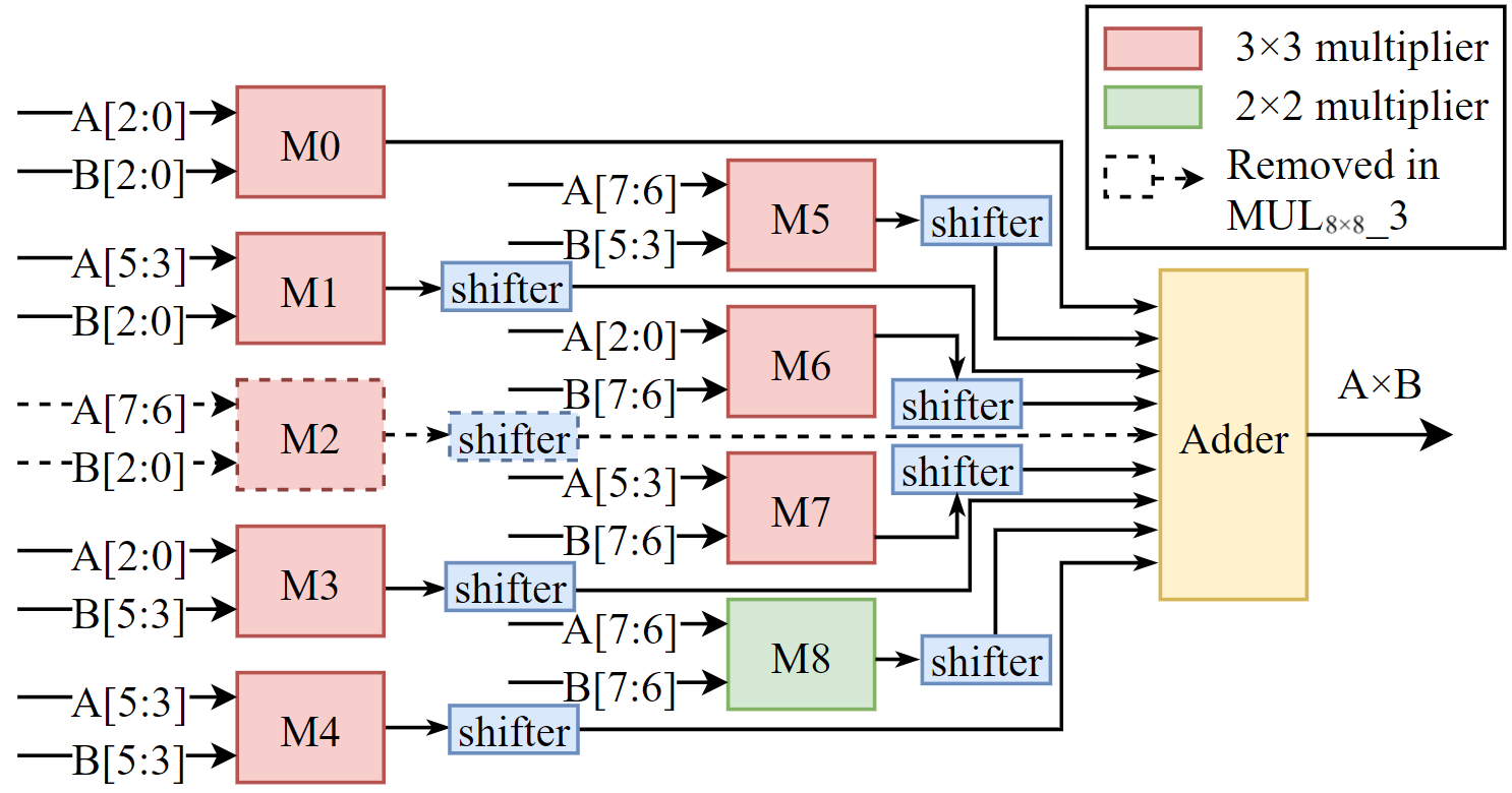
Figure 1: Block architecture of 8-bit multiplier based on 3×3 and 2×2 multipliers.

In addition, the DNN weights can be retrained to ensure that most weights are in (0, 31), where A[7:6] or B[7:6] is 00, so that we can remove M2 or M6 and the corresponding shifter from the architecture in Fig.1, which can further reduce the critical path delay and power consumption.

III Experimental Results of Multipliers

III-A Error metrics

In this paper, we use ED, MED, ER, NMED, and MRED as error metrics. ED, MED, and ER are presented in (1)-(3). NMED and MRED are defined as follows.

$$NMED=\frac{MED}{(2^{n}-1)^{2}}$$ (10)

$$MRED=\frac{ED}{Value^{\prime}\cdot 2^{n}}$$ (11)

TABLE V shows the metric values of three approximate multipliers proposed in Section II and the existing approximate multipliers. Average ER, MED, NMED and MRED of MUL_8×8_1,2,3 are 24.9%, 298, 0.46%, and 1.81%, respectively. Such advantages of low ER and NMED can greatly improve the precision.

TABLE V: Arithmetic Accuracy Comparision of Approximate Multipliers

Name	ER(%)	MED	NMED(%)	MRED(%)
MUL8×8_1	22.8	137.04	0.21	1.50
MUL8×8_2	20.49	114.83	0.18	1.42
MUL8×8_3	31.41	648.20	1.00	2.53
SiEi[7]	31.59	-	0.20	0.62
PKM[10]	49.86	938.32	1.44	3.89
ETM[12]	98.88	-	2.85	25.21
SV[21]	-	-	0.35	6.75

TABLE VI: Comparision of 3×3 Approximate Multipliers in terms of Area, Power, Delay

Types	Area( $\mu m^{2}$)	Power(mW)	Delay(ns)
	(Improvement)	(Improvement)	(Improvement)
Exact (baseline)	67.68	3.73	0.45
MUL3×3_1	43.20 (36.17%)	2.40 (35.66%)	0.26 (42.22%)
MUL3×3_2	46.44 (31.38%)	2.36 (36.73%)	0.26 (42.22%)

TABLE VII: Comparision of 8×8 Approximate Multipliers in terms of Area, Power, Delay

Types	Area( $\mu m^{2}$)	Power(mW)	Delay(ns)
	(Improvement)	(Improvement)	(Improvement)
Exact (baseline)	744.59	58.12	1.58
MUL8×8_1	596.16 (19.93%)	45.66 (21.44%)	1.29 (18.35%)
MUL8×8_2	646.92 (13.12%)	50.84 (12.53%)	1.41 (10.76%)
MUL8×8_3	571.32 (23.27%)	42.28 (27.25%)	1.29 (18.35%)
SiEi[7]	579.51 (22.17%)	39.57 (31.92%)	1.37 (13.29%)
PKM[10]	564.76 (24.15%)	37.87 (34.84%)	1.28 (18.99%)

TABLE VIII: DNN Results of Approximate Multipliers

Dataset	MNIST			CIFAR-10
Multiplier Type	LeNet	Regularization	LeNet+	LeNet	LeNet+	VGG16	AlexNet	ResNet-19
Exact(baseline)	99.32%	99.41%	99.51%	75.09%	76.80%	93.51%	88.48%	88.92%
MUL8×8_1	98.98%	99.02%	99.14%	60.84%	61.47%	29.59%	56.95%	39.84%
MUL8×8_2	99.32%	99.41%	99.51%	74.21%	77.00%	91.60%	88.17%	87.58%
MUL8×8_3	98.49%	99.12%	99.22%	54.70%	64.44%	31.32%	73.80%	73.76%
SiEi[7]	74.88%	95.46%	95.77%	12.56%	13.56%	9.80%	8.64%	10.59%
PKM[10]	96.32%	98.39%	98.40%	36.23%	47.05%	11.47%	37.95%	24.72%

Because the ER and MRED of ETM [12] are too poor to compare and SV[21] lacks ER and MED, we select the five approximate multipliers: MUL_8×8_1-3, SiEi[7] and PKM[10] to carry out the follow-up experimental evaluation.

III-B Results of 3$\times$3 Approximate Multipliers

In this part, all approximate multiplier architectures are written in Verilog, and synthesized by Synopsys Design Compiler (DC) with ASAP 7nm standard cell library[22] to obtain the area and power values. The DC results of 3×3 approximate multipliers are shown in TABLE VI. In comparison to the exact multiplier produced by Synopsys DesignWare library, MUL_3×3_1 and MUL_3×3_2 can reduce the area by 36.17% and 31.38% and power consumption by 35.66% and 36.73%, respectively. The delay can be reduced by 42.22%.

III-C Results of 8$\times$8 Approximate Multipliers

We can obtain DC results of 8×8 approximate multiplier as shown in TABLE VII, where MUL_8×8_1,2,3 can reduce the area by 19.93%, 13.12%, and 23.27%, respectively. The power consumption is reduced by 21.44%, 12.53%, and 27.25%, respectively. On the critical delay, the proposed designs can also reduce 18.35%, 10.76%, and 18.35%. In [10], PKM uses the approximate unit in MSBs, which can reduce the area, power, and delay to some extent. However, it leads to the high DAL as shown in the following Section IV.

IV DNN with Approximate Multipliers

In this section, the DNN platform[17] is extended to evaluate the DAL caused by replacing exact multipliers with approximate 8×8 multipliers. The 8-bit unsigned approximate multipliers in Section II are evaluated by this platform and compared with the exact multiplier. When the DNN accuracy is lower than 40%, we usually think that the network with approximate multipliers loses its predictive ability.

Under this platform, we train the DNN on the MNIST and CIFAR10 datasets, respectively. Based on the DNN structure, we can increase the number of convolution layers in LeNet to increase network complexity, which can also improve the recognition ability of the input layer. The modified LeNet structure can be denoted by LeNet+. And the tolerance of approximate multipliers in larger networks can be predicted.

On the MNIST, MUL_8×8_1,2,3 are good-performance approximation multipliers. Under the original LeNet structure, the worst DAL of our three designs is MUL_8×8_3 (0.83%), and the best one is MUL_8×8_2 (no accuracy loss).

We find that the retraining we applied can reduce the DAL of MUL_8×8_1,2,3 when compared to the baseline in TABLE VIII. Regularization and LeNet+ keep the DNN accuracy of MUL_8×8_2 at a high level and they can improve the DAL of the worst design to 0.39% and 0.37%, respectively. It also follows that LeNet+ has a better improvement than regularization. So we apply LeNet+ only on CIFAR10.

The original DNN accuracy of MUL_8×8_2 is similar to that of baseline on CIFAR10, and in LeNet+, it even exceeds the DNN accuracy of the exact multiplier. However, PKM, which has a moderate effect on MNIST, has only 36.23% DNN result on CIFAR10, which can reach 47.05% after retraining in LeNet+.

LeNet is sufficient for MNIST, but for CIFAR10, we need to use larger DNNs to evaluate the approximate multipliers. VGG16, AlexNet, and ResNet-19 are then adopted to our DNN platform. MUL_8×8_2 can obtain better DAL than other designs in our evaluation. It can be seen that the prediction unit in MUL_3×3_2 is very necessary, and it consumes a little extra area to achieve the improvement of accuracy. In addition to reproduced multipliers above, we choose another state-of-the-art multiplier to compare. The DAL of the multiplier design shown in[23] is 3.86% in VGG16 ($m=3$) on CIFAR10, while MUL_8×8_2 can obtain a lower DAL (1.91%).

V Conclusion

In this paper, we propose two 3×3 approximate multipliers, which have the same ER but different MEDs. Compared with the exact 3×3 multiplier, MUL_3×3_1,2 can reduce the area, power consumption, and delay by 33.5%, 36.1% and 42.2% on average, respectively. They are then aggregated with 2×2 multipliers into the 8×8 multiplier according to DNN weights, which is evaluated and co-optimized by the extended DNN platform. MUL_8×8_2 has no DAL for LeNet on MNIST dataset without retraining. On CIFAR10, MUL_8×8_2 even exceeds the DNN accuracy of exact multiplier on LeNet+. For ResNet-19, AlexNet, and VGG16, the DALs of MUL_8×8_2 are significantly smaller than those of other designs on CIFAR10. Overall, due to the hardware and software co-optimization, the DAL can be negligible with the proposed MUL_8×8_2.

References

- [1] J. Han and M. Orshansky, “Approximate computing: An emerging paradigm for energy-efficient design,” 18th IEEE European Test Symposium (ETS), Avignon, France, 2013, pp. 1-6.
- [2] Chandan Kumar Jha, Sumit Walia, Gagan Kanojia, Joycee Mekie, “FPCAM: Floating Point Configurable Approximate Multiplier for Error Resilient Applications,” IEEE International Symposium on Circuits and Systems (ISCAS), pp. 1-5, 2021.
- [3] John N. Mitchell, “Computer multiplication and division using binary logarithms,” IRE Transactions on Electronic Computers, vol. 4, pp. 512-517, 1962.
- [4] Z. Babić, A. Avramović and P. Bulić, “An iterative logarithmic multiplier,” Microprocessors and Microsystems, vol. 35, no. 1, pp. 23-33, 2011.
- [5] M. B. Sullivan and E. E. Swartzlander, “Truncated error correction for flexible approximate multiplication,” Proc. ASILOMAR, pp. 355-359, 2012.
- [6] Syed Ershad Ahmed, Sanket Kadam and M. B. Srinivas, “An Iterative Logarithmic Multiplier with Improved Precision,” IEEE 23nd Symposium on Computer Arithmetic (ARITH), 2016.
- [7] C. Liu, J. Han and F. Lombardi, “A low-power high-performance approximate multiplier with configurable partial error recovery,” Proc. Des. Autom. Test Europe Conf. Exhib., pp. 1-4, 2014.
- [8] R. Zendegani, M. Kamal, M. Bahadori, A. Afzali-Kusha and M. Pedram, “RoBA Multiplier: A Rounding-Based Approximate Multiplier for High-Speed yet Energy-Efficient Digital Signal Processing,” IEEE Transactions on Very Large Scale Integration (VLSI) Systems, vol. 25, no. 2, pp. 393-401, Feb. 2017.
- [9] K. Y. Kyaw, W. L. Goh, and K. S. Yeo, “Low-power high-speed multiplier for error-tolerant application,” in IEEE Intl. Conf. Electron Devices and Solid-State Circuits (EDSSC) , pp. 1-4, 2010.
- [10] P. Kulkarni, P. Gupta and M. Ercegovac, “Trading accuracy for power with an underdesigned multiplier architecture,” 24th International Conference on Very Large Scale Integration (VLSI) Design, pp. 346-351, 2011.
- [11] A. Momeni, J. Han, P. Montuschi, and F. Lombardi, “Design and analysis of approximate compressors for multiplication,” IEEE Trans. Comput., vol. 64, no. 4, pp. 984–994, Apr. 2015.
- [12] S. Venkatachalam and S.-B. Ko, “Design of power and area efficient approximate multipliers,” IEEE Transactions on Very Large Scale Integration (VLSI) Systems, 2017.
- [13] J. Liang, J. Han and F. Lombardi, “New metrics for the reliability of approximate and probabilistic adders,” IEEE Trans. Comput., vol. 62, no. 9, pp. 1760-1771, Sep. 2013.
- [14] I. Scarabottolo, G. Ansaloni, G. A. Constantinides, L. Pozzi and S. Reda, “Approximate Logic Synthesis: A Survey,” in Proceedings of the IEEE, vol. 108, no. 12, pp. 2195-2213, Dec. 2020.
- [15] B. Jacob et al., “Quantization and Training of Neural Networks for Efficient Integer-Arithmetic-Only Inference,” IEEE/CVF Conference on Computer Vision and Pattern Recognition, 2018.
- [16] Y. Chen, T. Yang, J. Emer and V. Sze, “Eyeriss v2: A Flexible Accelerator for Emerging Deep Neural Networks on Mobile Devices,” in IEEE Journal on Emerging and Selected Topics in Circuits and Systems, vol. 9, no. 2, pp. 292-308, June 2019.
- [17] J. Zhang, S. Zheng and L. Wang, “ApproxDNNFlow: An Evaluation and Exploration Framework for DNNs with Approximate Multipliers,” 2021 China Semiconductor Technology International Conference (CSTIC), pp. 1-3, 2021.
-
[18]
Y. LeCun and C. Cortes, “MNIST handwritten digit database,”
http://yann.lecun.com/exdb/mnist/ - [19] Krizhevsky, A. and Hinton, G., “Learning multiple layers of features from tiny images,” Handbook of Systemic Autoimmune Diseases, vol. 4, no. 1, 2009.
- [20] T. Thorsten, “Quine-McCluskey algorithm,” https://www.mathematik. uni-marburg.de/thormae/lectures/ti1/code/qmc/
- [21] S. Venkatachalam, H. J. Lee and S. Ko, “Power Efficient Approximate Booth Multiplier,” IEEE International Symposium on Circuits and Systems (ISCAS), 2018.
- [22] L. Clark, V. Vashishtha, L. Shifren, A. Gujja, S. Sinha, B. Cline, C. Ramamurthy, and G. Yeric, “ASAP7: A 7-nm finfet predictive process design kit,” July, 2016.
- [23] G. Zervakis, O. Spantidi,I. Anagnostopoulos and H. Amrouch, “Control Variate Approximation for DNN Accelerators,” 58th ACM/IEEE Design Automation Conference (DAC), 2021.