Empirical Bayes Selection for Value Maximization

Abstract

We study the problem of selecting the best $m$ units from a set of $n$ as $m/n\to\alpha\in(0,1)$, where noisy, heteroskedastic measurements of the units’ true values are available and the decision-maker wishes to maximize the average true value of the units selected. Given a parametric prior distribution, the empirical Bayes decision rule incurs $\mathcal{O}_{p}(n^{-1})$ regret relative to the Bayesian oracle that knows the true prior. More generally, if the error in the estimated prior is of order $\mathcal{O}_{p}(r_{n})$, regret is $\mathcal{O}_{p}(r_{n}^{2})$. In this sense selecting the best units is easier than estimating their values. We show this regret bound is sharp in the parametric case, by giving an example in which it is attained. Using priors calibrated from a dataset of over four thousand internet experiments, we find that empirical Bayes methods perform well in practice for detecting the best treatments given only a modest number of experiments.

1 Introduction

In many important scientific and economic applications, decision-makers are presented with data on the performance of $n$ units, from which they must select a strict subset for further investigation or treatment. Examples include identifying the best teachers, hospitals, or athletes [6, 17, 11]; genes associated with particular outcomes [23]; drug candidates [62]; or, in the application we consider in this paper, the treatments in internet experiments with the largest effects on a metric of interest. Each unit is associated with an unobserved true value, which is measured with heteroskedastic noise. The constraint that only $m$ units can be selected arises naturally when the decision-maker has limited resources to devote to the chosen units, and must restrict attention to the most promising candidates.

A desirable feature of a selection procedure is that the aggregate value of its selections is close to the maximum attainable value. Understanding how different selection procedures perform in this respect enables decision-makers to assess how likely they are to succeed in the preceding applications. The empirical Bayes approach to this question involves estimating the unknown, prior distribution from which the true values are drawn, and selecting units with the highest estimated posterior means. We show that if the prior distribution is known to lie within some parametric class, empirical Bayes incurs regret of order $\mathcal{O}_{p}(n^{-1})$ relative to the oracle Bayes procedure in which the prior distribution is known. This is faster than the usual $n^{-1/2}$ rate of convergence in parametric models. In this sense selection is easier than estimation: picking the set of units with the highest values is easier than pinning down the precise values of those units. This generalizes directly to the nonparametric case: regret converges to zero at the square of the rate that estimation error in the prior converges to zero.

The basic intuition for this result is as follows. First, mistakes, whether of inclusion or exclusion, are only likely to happen for those units whose true values are sufficiently close to a critical threshold. Units comfortably (or below) above that threshold will be correctly selected (or omitted) with high probability (w.h.p.). Second, even those mistakes cannot be too costly, as items incorrectly included or excluded are likely to be marginal — almost good enough to be selected, or almost bad enough to be omitted. The regret, which is the product of two terms corresponding to these factors, will therefore be second-order small. We show that our $\mathcal{O}_{p}(n^{-1})$ bound is sharp in the parametric case, by constructing an example in which regret is at least $Cn^{-1}$ with non-vanishing probability for some positive constant $C$.

We apply this methodology to internet experimentation, where units correspond to experiments, and values to treatment effects. Heteroskedasticity arises because experiments vary in sample size. Technology companies may wish to identify a subset of best- or worst-performing experiments for further investigation, in the former case, as candidates to launch to production, or in the latter case, as candidates to stop early. When the follow-up investigation incurs some cost, it may only be feasible to select a strict subset of experiments for more analysis. In this application, as in others, the cost of mistakes depends on their magnitude, that is, on the difference between the aggregate value of the units selected and the units that should have been selected.

The oracle Bayes decision rule assumes knowledge of the prior distribution of treatment effects. Given the objective of maximizing the expected aggregate values of the selection, the optimal procedure is to select the $m$ units with treatment effects with the highest posterior means. The empirical Bayes approach differs from this only in using the estimated prior instead of the true prior. We compare the performance of the empirical and oracle Bayes procedures in selecting the top $10\%$ of experiments from a sample of $4677$. We estimate the prior distribution of true effects with a scale mixture of mean-zero Gaussians, fitted with ebnm [61]. Treating the estimated prior as the truth, we simulate new experiments’ true and estimated treatment effects, and evaluate the regret of the empirical Bayes approach on this semi-synthetic data. Consistent with our theoretical results, we find that regret is $\mathcal{O}_{p}(n^{-1})$. By comparison, identifying the set of the top $10\%$ experiments with all misclassifications being equally penalized regardless of their magnitude, or estimating the treatment effects of the selected experiments, or estimating the prior distribution itself, are all categorically harder problems, each of which only exhibits convergence at the usual parametric rate.

Our work builds on several large and active strands of the statistics and econometrics literature. Foundational work introducing and developing the empirical Bayes approach to statistics includes [51, 41, 52, 21]. Applications of the selection problem have proliferated, as the general problem of discerning between units which perform well or poorly on the basis of noisy, heteroskedastic measurements describes many real-world settings of interest. Previous work has studied identifying the best teachers [39, 38, 35, 10, 25], the best medical facilities [56, 27, 17, 36], the best baseball players [22, 6]; differentially expressed genes [23, 54]; promising drug candidates [62]; geographic areas associated with the greatest intergenerational mobility [4] or mortality [46], and employers exhibiting the most evidence of discrimination [42]. Internet experiments are particularly well-suited to empirical Bayes methods [15, 26, 2, 12, 3, 30] as datasets are often large enough for accurate estimation of flexibly-specified priors, and the experiment-level sampling error is typically close to normally distributed. For these applications, the aggregate value of the selected units will often be an important component of the decision-maker’s utility function. Our results provide theoretical and empirical support for selection based on such methods.

The literature on post-selection inference, including [14, 13, 33, 24, 37, 1, 31], also studies selection problems, but differs from the present work in that its chief focus is estimating the values, differences or ranks of the selected units, rather than analyzing the regret associated with the selection. [14, 13] provide estimates for the value of a selection unit. [33, 24, 37, 1, 31] largely aim at frequentist inferences. While the notion of regret we consider averages over possible draws from the distribution of units’ true values, an alternative line of inquiry beyond the scope of this paper would be to characterize admissible and minimax decision rules for the frequentist analog of the regret we define, considering the units’ values as fixed constants.

Closely related to our paper are [29, 49]. [29] take an empirical Bayes approach to selecting the best units while controlling the marginal false discovery rate; [49] assert frequentist control over the familywise error rate, which amounts to a zero-one loss based on the correctness of the ranks. Both consider loss functions different from ours. In their frameworks, the loss function contains a discontinuity near the oracle Bayes decision rule, e.g. [29, Equation 3.1]. Mistakenly selecting or omitting any unit incurs a discrete cost, whereas in ours the cost of mistakenly selecting or omitting a marginal unit near the selection threshold is small, see also [29, Section 3.2]. We view these as complementary perspectives. While in some decision problems mistakes may be undesirable per se, the aggregate performance of the selected units is typically still a relevant consideration. In the context of teacher evaluation, for example, the policy-maker may rightly be concerned with guarantees over the number of teachers who are incorrectly fired [48], but may also wish to understand how well their selection procedure is performing from the students’ perspective, in terms of the aggregate “value-added” of the teachers who keep their jobs. In other contexts, as in internet experimentation or drug discovery, the aggregate value of the selection is the primary concern, and it is harder to justify caring about the number of mistakes per se.

Our selection problem may remind readers of the multi-armed bandit literature, e.g. [53, 9] study the problem of identifying the best arm or best $m$ arms at a certain probability. However to target the probability of correct selection is to consider discontinuous loss functions similar to ones in [29, 49]. We also note that our selection problem is non-sequential which leads to new challenges, as poor choices of parameter in the prior cannot be overcome with additional samples in long run.

Finally, our work is particularly tied to the framework introduced in [59], which generalizes the restrictive compound decision framework from [34] to a class of simultaneous decision problems that are permutation invariant. However the optimal frequentist solution requires knowledge of the empirical c.d.f. (e.c.d.f.), or equivalently the order statistic, of the $\mu_{i}$’s. Thus for practical reasons, we take a more Bayesian approach that also allows analysis of the performance.

Our main contribution relative to this existing literature is to provide the first regret bounds for empirical Bayes selection, and further to show that these bounds are sharp in the parametric case. Our empirical work on internet experimentation complements this by verifying that regret is quantitatively modest in practice, given a reasonable number experiments of moderate precision. Together, our theoretical and empirical results suggest optimism for empirical Bayes approaches to selection when the decision-maker is primarily concerned with maximizing the aggregate value of the selected units, as opposed to correctly classifying the top units or estimating their values.

2 The Top-$m$ Selection Problem

2.1 Setup

There are $n$ units, each of which is associated with a unobserved true value $\mu_{i}\in\mathbb{R}$ and an observed noise standard deviation $\sigma_{i}>0$. The $\mu_{i}$ and $\sigma_{i}$ are distributed independently from each other and independently across experiments with unknown marginal distributions $G_{0}$ and $H_{0}$, i.e.

$$(\mu_{i},\sigma_{i})\sim G_{0}\times H_{0}.$$

We consider a potentially nonparametric family of nondegenerate prior distributions $G(\eta)$, where the parameter $\eta$ belongs to a metric space $(\mathcal{M},d)$, and the family includes the truth $G_{0}$, i.e. $G_{0}=G(\eta_{0})$ for some $\eta_{0}\in\mathcal{M}$. For each unit $i$, the decision-maker observes a measurement $X_{i}\in\mathbb{R}$, which is distributed as

$$X_{i}\mid\mu_{i},\sigma_{i}\sim\mathcal{N}(\mu_{i},\sigma_{i}^{2}).$$

The decision-maker must choose $m$ units for some $m<n$. Their average utility given the index set of choices $J\subset\{1,2,\ldots,n\}$ is $U(J)=\frac{1}{n}\sum_{i=1}^{n}\mathbb{1}(i\in J)\mu_{i}$. Let

$$f_{\eta,\sigma_{i}}(X_{i})=\frac{\int\mu\frac{1}{\sigma_{i}}\phi\left(\frac{X_{i}-\mu}{\sigma_{i}}\right)\,dG(\eta)}{\int\frac{1}{\sigma_{i}}\phi\left(\frac{X_{i}-\mu}{\sigma_{i}}\right)\,dG(\eta)}$$ (1)

denote the posterior mean of $\mu_{i}$ given $X_{i},\sigma_{i}$, assuming that the prior distribution of $\mu_{i}$ is $G(\eta)$, where $\phi(\cdot)$ is the probability density function (p.d.f.) of a standard Gaussian. The true posterior mean is $f_{\eta_{0},\sigma_{i}}(X_{i})$. An estimator $\widehat{\eta}=\widehat{\eta}(X_{1},\ldots,X_{n},\allowbreak\sigma_{1},\ldots,\sigma_{n})$ of $\eta_{0}$ is available, where $\widehat{\eta}$ converges to $\eta_{0}$ at some rate $r_{n}$ in $d(\cdot,\cdot)$. It is used to form the empirical Bayes prior, $G(\widehat{\eta})$, and consequently to construct posterior mean estimates, $f_{\widehat{\eta},\sigma_{i}}(X_{i})$. For simplicity we denote $f_{\eta_{0},\sigma_{i}}(X_{i})$ and $f_{\widehat{\eta},\sigma_{i}}(X_{i})$, the oracle and empirical Bayes posterior means for unit $i$, as $\theta_{i}$ and $\widehat{\theta}_{i}$ respectively. Note we can view $\theta_{i}$ as being drawn i.i.d. from a distribution, which we denote $P$.

Given the observed data, an oracle Bayesian decision-maker maximizes expected utility (where the expectation is with respect to the posterior distribution over the unknown true values) by selecting the $m$ units with the highest values of $\theta_{i}$, breaking ties randomly. The empirical Bayes decision-maker mimics this rule, by selecting the $m$ units with the highest values of $\widehat{\theta}_{i}$, breaking ties randomly. Letting $J_{\text{EB}}$ and $J_{\text{Bayes}}$ be the empirical Bayes and oracle Bayes choice sets, the regret from empirical relative to oracle Bayes is

$$\mathcal{R} =\mathbb{E}[U(J_{\text{Bayes}})\mid X_{1},\ldots,X_{n},\sigma_{1},\ldots,\sigma_{n}]-\mathbb{E}[U(J_{\text{EB}})\mid X_{1},\ldots,X_{n},\sigma_{1},\ldots,\sigma_{n}]$$

$$=\frac{1}{n}\sum_{i=1}^{n}(\mathbb{1}(i\in J_{\text{Bayes}})-\mathbb{1}(i\in J_{\text{EB}}))\theta_{i},$$ (2)

where $\mathbb{1}(\cdot)$ is the indicator function. We aim to characterize how quickly $\mathcal{R}$ converges to zero as $n\to\infty$. The proof that $\mathcal{R}=\mathcal{O}_{p}(r_{n}^{2})$ proceeds by bounding the regret $\mathcal{R}$ by the product of two terms: the proportion of mistakes, and the maximum possible magnitude of the loss caused by a mistake. We show that each of these terms are of the same order as the estimation error in $\widehat{\eta}$, and consequently regret must be second-order small, i.e. $\mathcal{O}_{p}(r_{n})\cdot\mathcal{O}_{p}(r_{n})=\mathcal{O}_{p}(r_{n}^{2})$.

Note that in the homoskedastic case when all the variances are equal, i.e. $\sigma_{1}=\cdots=\sigma_{n}$, the posterior mean of $\mu_{i}$ is monotone in $X_{i}$ for any choice of prior [19, 43]. Hence the Bayes selection rule amounts to selecting the top-$m$ observations, and this selection problem is trivial.

2.2 Establishing a Convergence Bound

To establish a convergence bound, we enlist Assumptions 1, 2 and 3.

Assumption 1.

$d(\widehat{\eta},\eta_{0})=\mathcal{O}_{p}(r_{n})$ for some sequence $(r_{n})_{n\in\mathbb{N}}$ with $r_{n}\geq n^{-1/2}$ for all $n$.

Assumption 2.

The support of the distribution $H_{0}$ of $\sigma_{i}$ is compact and bounded away from $0$.

Assumption 3.

The mapping $\eta\mapsto G(\eta)$ is locally Lipschitz with respect to $1$-Wasserstein distance, $W_{1}(\cdot,\cdot)$, in the codomain.

Assumption 1 will be satisfied under mild conditions by the maximum likelihood estimator for a finite-dimensional parameter $\eta$, with $r_{n}=n^{-1/2}$ [40, Theorem 9.14]. This includes the commonly used “normal-normal” model, in which the prior is $\mathcal{N}(m_{g},v_{g})$ for unknown $m_{g},v_{g}$ which can be estimated by maximizing the likelihood. In the nonparametric case we will generally obtain slower rates of convergence, as allowed for by this assumption. For example, from the existing literature on convergence rates for deconvolution problems:

• if the prior takes on some finite but unknown number of values, [8] shows that the best possible convergence rate for estimating the prior in the $1$-Wasserstein metric is $n^{-1/4}$;

• if the prior has a density function with $k$ bounded derivatives, [7] shows that the fastest rate of convergence of any estimator of the prior is $(\log n)^{-k/2}$ in the $L_{1}$-norm of the p.d.f.. Furthermore, if we assume the support of $G(\eta)$ is bounded, the same rate of convergence applies to the $1$-Wasserstein metric.

Assumption 2 states that there are non-trivial upper and lower bounds on the precision with which the true values are measured, as would be the case in experiments with sample sizes bounded below and above. Assumption 3 is a relatively weak regularity condition which will be used to show that the posterior means depend continuously on the prior. The $1$-Wasserstein metric is a natural choice here: other common statistical distances such as total variation distance or Kullback–Leibler divergence have no regard to the metric on the observation space, or require the distributions to be absolutely continuous. In the parametric case, Assumption 3 is satisfied by common families such as finite mixture families parameterized only by their weights and canonical exponential families with finite variance. In the nonparametric case, the parameter $\eta$ can itself be taken to be the prior distribution, and the assumption is trivially satisfied with Lipschitz constant $1$. Finally, Assumption 3 can be further weakened to requiring local Lipschitz continuity only at $\eta_{0}$ by restricting the parameter space $\mathcal{M}$ appropriately, which we omit in this paper for easier exposition.

Under these assumptions, our main result follows.

Theorem 1.

If Assumptions 1, 2 and 3 hold, then $\mathcal{R}=\mathcal{O}_{p}(r_{n}^{2})$, the square of the rate of convergence for estimating the prior.

We give a brief overview of the proof strategy behind this theorem, before establishing the required supporting lemmas and giving the proof itself. Regret arises because our estimated posterior means, $\widehat{\theta}_{i}$, are different from their oracle Bayes counterparts, $\theta_{i}$, and consequently the top units ranked by the former may differ from the top units ranked by the latter. The difference between $\widehat{\theta}_{i}$ and $\theta_{i}$ is the shrinkage error for observation $i$. We show that regret can be bounded above by the product of the maximum magnitude of the shrinkage error from mistakes (whether of inclusion or exclusion) and the proportion of such mistakes. It suffices to show that each of these terms is $\mathcal{O}_{p}(r_{n})$. Using the facts that the posterior mean function $f_{\eta,\sigma}(X_{i})$ is sufficiently well-behaved around the $\eta_{0}$ when the observations $X_{i}$ belong to a compact set (Lemma 3), and that the $X_{i}$’s associated with all mistakes lie within a compact set w.h.p. (Lemma 4), we can show that the maximum magnitude of the shrinkage error from mistakes is bounded above by a constant times $d(\widehat{\eta},\eta_{0})$, and hence is $\mathcal{O}_{p}(r_{n})$ by Assumption 1. Next we argue that for any neighborhood around $P^{-1}(1-\frac{m}{n})$ shrinking slower than $r_{n}$, the true values associated with mistakes will lie within that neighborhood w.h.p.. This allows us to control the proportion of mistakes, and conclude that they are also $\mathcal{O}_{p}(r_{n})$.

For proving Theorem 1, the following lemma is a key intermediate result, establishing continuity of both the posterior mean function $f_{\eta,\sigma}(X)$ and its inverse with respect to $X$. It will be used to argue that small deviations of $\eta$ around $\eta_{0}$ result in small deviations of $f_{\eta,\sigma}(X)$ around $f_{\eta_{0},\sigma}(X)$ (in a sense made precise in Lemma 3), and that the observations associated with mistakes must belong to a fixed compact set w.h.p. in Lemma 4. The existence of the inverse is given by Lemma 6, and essentially follows immediately from a classic result by [19].

Lemma 2.

Under Assumptions 2 and 3, the posterior mean function $f_{\eta,\sigma}(X)$ and its inverse $f^{-1}_{\eta,\sigma}(X)$ are both continuous in $(\eta,\sigma,X)\in\mathcal{M}\times\operatorname{supp}(H_{0})\times\mathbb{R}$.

Proof.

We first prove that $f_{\eta,\sigma}(X)$ is continuous in $(\eta,\sigma,X)$. From (1),

$$f_{\eta,\sigma}(X)=\frac{\int\mu\frac{1}{\sigma}\phi\left(\frac{X-\mu}{\sigma}\right)\,dG(\eta)}{\int\frac{1}{\sigma}\phi\left(\frac{X-\mu}{\sigma}\right)\,dG(\eta)}=\frac{\int\mu\phi\left(\frac{X-\mu}{\sigma}\right)\,dG(\eta)}{\int\phi\left(\frac{X-\mu}{\sigma}\right)\,dG(\eta)}\coloneqq\frac{h_{1}(\eta,\sigma,X)}{h_{0}(\eta,\sigma,X)},$$ (3)

where $\phi(\cdot)$ is the p.d.f. of a standard Gaussian. As $h_{0}>0$, it suffices to show that $h_{0}$ and $h_{1}$ are continuous.

Suppose we have a sequence $(\eta_{k},\sigma_{k},X_{k})\to(\eta^{*},\sigma^{*},X^{*})$ as $k\to\infty$. For $h_{1}$, we wish to show that

$$\int\mu\phi\left(\frac{X_{k}-\mu}{\sigma_{k}}\right)\,dG(\eta_{k})\to\int\mu\phi\left(\frac{X^{*}-\mu}{\sigma^{*}}\right)\,dG(\eta^{*}).$$

Note that the function sequence $\mu\phi\left(\frac{X_{k}-\mu}{\sigma_{k}}\right)$ converges uniformly to $\mu\phi\left(\frac{X^{*}-\mu}{\sigma^{*}}\right).$ Hence for any $\varepsilon>0$, when $k$ is sufficiently large, we have

$$~{}\left|\int\mu\phi\left(\frac{X_{k}-\mu}{\sigma_{k}}\right)\,dG(\eta_{k})-\int\mu\phi\left(\frac{X^{*}-\mu}{\sigma^{*}}\right)\,dG(\eta_{k})\right|$$

$$\leq ~{}\sup_{\mu\in\mathbb{R}}\left|\mu\phi\left(\frac{X_{k}-\mu}{\sigma_{k}}\right)-\int\mu\phi\left(\frac{X^{*}-\mu}{\sigma^{*}}\right)\right|$$

$$< ~{}\varepsilon/2.$$ (4)

Note also that $\mu\phi\left(\frac{X^{*}-\mu}{\sigma^{*}}\right)$ is Lipschitz. Therefore by Kantorovich–Rubinstein duality, when $k$ is sufficiently large, $W_{1}(G(\eta_{k}),G(\eta^{*}))$ is sufficiently small and

$$\left|\int\mu\phi\left(\frac{X^{*}-\mu}{\sigma^{*}}\right)\,dG(\eta_{k})-\int\mu\phi\left(\frac{X^{*}-\mu}{\sigma^{*}}\right)\,dG(\eta^{*})\right|<\varepsilon/2.$$ (5)

Summing up (4) and (5) yields the convergence of the numerator. The proof for $h_{0}$ is almost identical, as $\phi\left(\frac{X_{k}-\mu}{\sigma_{k}}\right)$ converges uniformly to $\phi\left(\frac{X^{*}-\mu}{\sigma^{*}}\right)$ and $\phi\left(\frac{X^{*}-\mu}{\sigma^{*}}\right)$ is Lipschitz. The continuity of $f_{\eta,\sigma}^{-1}(X)$ follows from the continuity of $f_{\eta,\sigma}(X)$ by Lemmas 6 and 8. ∎

Next we show that the posterior mean function $f_{\eta,\sigma}(X)$ is locally Lipschitz around $\eta_{0}$, uniformly in $(\sigma,X)\in\operatorname{supp}(H_{0})\times W$. This will be used in Theorem 1 to bound the shrinkage error by a constant times the estimation error in the prior parameter, $\widehat{\eta}$.

Lemma 3.

Suppose Assumptions 2 and 3 hold. Then for any compact $W\subset\mathbb{R}$, there exist positive constants $K$, $\delta$ such that for all $(\eta,\sigma,X)\in\mathcal{M}\times\operatorname{supp}(H_{0})\times W$, we have $|f_{\eta,\sigma}(X)-f_{\eta_{0},\sigma}(X)|\leq Kd(\eta,\eta_{0})$ whenever $d(\eta,\eta_{0})<\delta$.

Proof.

Using the same definition for $h_{0}$ and $h_{1}$ as in (3), we have

$$~{}|f_{\eta,\sigma}(X)-f_{\eta_{0},\sigma}(X)|$$

$$= ~{}\left|\frac{h_{1}(\eta,\sigma,X)}{h_{0}(\eta,\sigma,X)}-\frac{h_{1}(\eta_{0},\sigma,X)}{h_{0}(\eta_{0},\sigma,X)}\right|$$

$$\leq ~{}\frac{\left|h_{1}(\eta,\sigma,X)-h_{1}(\eta_{0},\sigma,X)\right|}{h_{0}(\eta,\sigma,X)}+\frac{\left|h_{1}(\eta_{0},\sigma,X)\right|\cdot\left|h_{0}(\eta_{0},\sigma,X)-h_{0}(\eta,\sigma,X)\right|}{h_{0}(\eta,\sigma,X)h_{0}(\eta_{0},\sigma,X)}.$$

It remains to show the following claims for when $\eta$ is in a sufficiently small neighborhood of $\eta_{0}$:

• $h_{0}$ is bounded away from $0$: Since $h_{0}$ is continuous from the proof of Lemma 2, $h_{0}(\eta_{0},\sigma,X)$ is strictly positive and $\operatorname{supp}(H_{0})\times W$ is compact, for sufficiently small $\delta$, $h_{0}(\eta,\sigma,X)$ is bounded away from $0$ whenever $d(\eta,\eta_{0})<\delta$.

• $h_{1}$ is Lipschitz in $\eta$ with a Lipschitz constant that does not depend on $\sigma$ or $X$: The integrand in $h_{1}$ is $\mu\phi\left(\frac{X-\mu}{\sigma}\right)$, a Lipschitz function in $\mu$. Since this Lipschitz constant is a continuous function in $\sigma,X$ and $\operatorname{supp}(H_{0})\times W$ is compact, $\mu\phi\left(\frac{X-\mu}{\sigma}\right)$ is uniformly Lipschitz. The function $h_{1}$ is Lipschitz in $G(\eta)$ again by Kantorovich–Rubinstein duality, and hence Lipschitz in $\eta$ as well.

• $h_{1}(\eta_{0},\sigma,X)$ is bounded: From the proof of Lemma 2, $h_{1}$ and thus $h_{1}(\eta_{0},\cdot,\cdot)$ are bounded. So $h_{1}(\eta_{0},\sigma,X)$ is bounded since $\operatorname{supp}(H_{0})\times W$ is compact. ∎

We will be applying Lemma 3 on a specific $W$ which will contain all of the observations corresponding to mistakes made by empirical Bayes selection w.h.p.. This is the subject of the following lemma. Recall the notation that $\triangle$ is the symmetric difference, so $J_{\text{Bayes}}\triangle J_{\text{EB}}$ is the index set of all mistakes.

Lemma 4.

If Assumptions 1, 2 and 3 hold, there exists a compact set $W$ such that $X_{i}\in W$ for all $i\in J_{\text{Bayes}}\triangle J_{\text{EB}}$ w.h.p..

Proof.

Oracle Bayesian selection essentially thresholds on $\theta^{*}$, the $m$-th largest order statistic of the $\theta_{i}$’s. For any $c>0$, this threshold lands in $(P^{-1}(1-\frac{m}{n})-c,P^{-1}(1-\frac{m}{n})+c)$ w.h.p. and hence $(P^{-1}(1-\alpha)-c,P^{-1}(1-\alpha)+c)$ w.h.p., by [57, Corollary 21.5 and discussion thereof]. Let $V$ be a open ball of $\eta_{0}$ whose radius is fixed but to be determined later. By Assumption 1, $\widehat{\eta}$ lies in $V$ w.h.p.. For any $i\notin J_{\text{EB}}$, under the high probability event $A_{n}$ defined as $A_{n}=\{\theta^{*}\in(P^{-1}(1-\alpha)-c,P^{-1}(1-\alpha)+c)\}\cap\{\widehat{\eta}\in V\}$,

$$\widehat{\theta}_{i} \leq\max_{\sigma^{\prime}\in\operatorname{supp}(H_{0})}f_{\widehat{\eta},\sigma^{\prime}}(f^{-1}_{\eta_{0},\sigma^{\prime}}(P^{-1}(1-\alpha)+c))$$ (6)

$$X_{i} \leq\max_{\sigma^{\prime}\in\operatorname{supp}(H_{0})}f^{-1}_{\widehat{\eta},\sigma_{i}}(f_{\widehat{\eta},\sigma^{\prime}}(f^{-1}_{\eta_{0},\sigma^{\prime}}(P^{-1}(1-\alpha)+c)))$$ (7)

$$\leq\max_{\sigma^{\prime},\sigma^{\prime\prime}\in\operatorname{supp}(H_{0})}f^{-1}_{\widehat{\eta},\sigma^{\prime\prime}}(f_{\widehat{\eta},\sigma^{\prime}}(f^{-1}_{\eta_{0},\sigma^{\prime}}(P^{-1}(1-\alpha)+c)))$$ (8)

By Lemma 6, the posterior mean function $f^{-1}_{\widehat{\eta},\sigma_{i}}$ is a strictly increasing function, so applying to both sides of (6) yields (7). Note that the maximand in (8) is a composition of functions in $\widehat{\eta},\sigma^{\prime},\sigma^{\prime\prime}$ that are continuous by Lemma 2, hence also a continuous function itself. By maximum theorem and the compactness of $\operatorname{supp}(H_{0})$, (8) is continuous in $\widehat{\eta}$ and locally bounded. In other words, for a sufficiently small open ball $V$ centered at $\eta_{0}$, (8) is bounded by some constant.

On the other hand, for any $i\in J_{\text{Bayes}}$, under the event $A_{n}$,

$$X_{i}=f^{-1}_{\eta_{0},\sigma_{i}}(\theta_{i}) \geq f^{-1}_{\eta_{0},\sigma_{i}}(P^{-1}(1-\alpha)-c)$$

$$\geq\min_{\sigma^{\prime}\in\operatorname{supp}(H_{0})}f^{-1}_{\eta_{0},\sigma^{\prime}}(P^{-1}(1-\alpha)-c).$$

Together, there exists a constant bounded interval that contains all $i$ in $J_{\text{Bayes}}\setminus J_{\text{EB}}$ under the event $A_{n}$. Likewise, there is also a constant bounded interval contains all $i$ in $J_{\text{EB}}\setminus J_{\text{Bayes}}$ under the event $A_{n}$. Taking $W$ to be the union of these two intervals completes the proof. ∎

Now we are ready to prove our main result, restated below.

See 1

Proof.

We first decompose an upper bound for $\mathcal{R}$ into two components.

$$\mathcal{R} =\frac{1}{n}\sum_{i=1}^{n}(\mathbb{1}(i\in J_{\text{Bayes}})-\mathbb{1}(i\in J_{\text{EB}}))\theta_{i}$$

$$\leq\frac{1}{n}\sum_{i=1}^{n}(\mathbb{1}(i\in J_{\text{Bayes}})-\mathbb{1}(i\in J_{\text{EB}}))\theta_{i}-\frac{1}{n}\sum_{i=1}^{n}(\mathbb{1}(i\in J_{\text{Bayes}})-\mathbb{1}(i\in J_{\text{EB}}))\widehat{\theta}_{i}$$ (9)

$$=\frac{1}{n}\sum_{i=1}^{n}(\mathbb{1}(i\in J_{\text{Bayes}})-\mathbb{1}(i\in J_{\text{EB}}))(\theta_{i}-\widehat{\theta}_{i})$$

$$\leq\frac{1}{n}\#(J_{\text{Bayes}}\triangle J_{\text{EB}})\cdot\max_{i\in J_{\text{Bayes}}\triangle J_{\text{EB}}}|\theta_{i}-\widehat{\theta}_{i}|$$

$$=2\cdot\underbrace{\frac{1}{n}\#(J_{\text{Bayes}}\setminus J_{\text{EB}})}_{\text{Proportion of mistakes}}\cdot\underbrace{\max_{i\in J_{\text{Bayes}}\triangle J_{\text{EB}}}|\theta_{i}-\widehat{\theta}_{i}|}_{\text{Maximum magnitude of shrinkage error}},$$ (10)

where (9) follows from the fact that $J_{\text{EB}}$ is the set of indices of the $m$ largest $\widehat{\theta}_{i}$’s. From (10), it suffices to bound the proportion of mistakes and the maximum magnitude of shrinkage error.

We start by bounding the latter term. We denote the that the observations associated with all mistakes belong in the set $W$ from Lemma 4 and $\widehat{\eta}$ belongs to a neighborhood $V$ around $\eta_{0}$ by $A_{n}=\{X_{i}\in W\text{ for all }i\in J_{\text{Bayes}}\triangle J_{\text{EB}}\}\cap\{\widehat{\eta}\in V\}$. By Lemma 4, $\mathbb{P}(A_{n})\to 1$, and under this high probability event, we have

$$\max_{i\in J_{\text{Bayes}}\triangle J_{\text{EB}}}|\theta_{i}-\widehat{\theta}_{i}| =\max_{i\in J_{\text{Bayes}}\triangle J_{\text{EB}}}|f_{\eta_{0},\sigma_{i}}(X_{i})-f_{\widehat{\eta},\sigma_{i}}(X_{i})|$$

$$\leq\max_{\begin{subarray}{c}X\in W\\ \sigma\in\operatorname{supp}(H_{0})\end{subarray}}|f_{\eta_{0},\sigma}(X)-f_{\widehat{\eta},\sigma}(X)|$$

$$\leq Kd(\eta_{0},\widehat{\eta}).$$ (11)

(11) follows from Lemma 3, and is $\mathcal{O}_{p}(r_{n})$ by Assumption 1. Consequently

$$\max_{i\in J_{\text{Bayes}}\triangle J_{\text{EB}}}|\theta_{i}-\widehat{\theta}_{i}|=\mathcal{O}_{p}(r_{n}).$$ (12)

Next we bound the proportion of mistakes. For any nondecreasing sequence $(b_{n})_{n\in\mathbb{N}}$ with $\lim_{n\to\infty}b_{n}=\infty$, we define the event $B_{n}$ as

$$B_{n}=\left\{\max_{i\in J_{\text{Bayes}}\setminus J_{\text{EB}}}\left|\theta_{i}-P^{-1}\left(1-\frac{m}{n}\right)\right|\leq b_{n}r_{n}\right\}.$$

Then

$$\frac{1}{n}\#(J_{\text{Bayes}}\setminus J_{\text{EB}})\leq\mathbb{1}(B_{n}^{c})+\mathbb{1}(B_{n})\frac{1}{n}\#\left\{i:\left|\theta_{i}-P^{-1}\left(1-\frac{m}{n}\right)\right|\leq b_{n}r_{n}\right\}.$$

We will first argue that $\mathbb{P}(B_{n}^{c})\rightarrow 0$ and then that $\frac{1}{n}\#\{i:|\theta_{i}-P^{-1}(1-\frac{m}{n})|\leq b_{n}r_{n}\}=\mathcal{O}_{p}(b_{n}r_{n})$, giving $\frac{1}{n}\#(J_{\text{Bayes}}\setminus J_{\text{EB}})=\mathcal{O}_{p}(b_{n}r_{n})$. Since $(b_{n})_{n\in\mathbb{N}}$ was an arbitrary nondecreasing sequence converging to infinity, by Lemma 9 this implies $\frac{1}{n}\#(J_{\text{Bayes}}\setminus J_{\text{EB}})=\mathcal{O}_{p}(r_{n})$.

For each $i$ in $J_{\text{Bayes}}\setminus J_{\text{EB}}$, empirical Bayes selection must have excluded it because some other shrinkage estimate was larger, i.e. $\widehat{\theta}_{i}\leq\widehat{\theta}_{i^{\prime}}$ for some $i^{\prime}\in J_{\text{EB}}\setminus J_{\text{Bayes}}$. Hence for each $i\in J_{\text{Bayes}}\setminus J_{\text{EB}}$, there is a $i^{\prime}\in J_{\text{EB}}\setminus J_{\text{Bayes}}$ such that

$$\theta^{*}\leq\theta_{i}\leq\theta_{i^{\prime}}+2\max_{i\in J_{\text{Bayes}}\triangle J_{\text{EB}}}|\theta_{i}-\widehat{\theta}_{i}|\leq\theta^{*}+2\max_{i\in J_{\text{Bayes}}\triangle J_{\text{EB}}}|\theta_{i}-\widehat{\theta}_{i}|,$$

and so

$$\max_{i\in J_{\text{Bayes}}\setminus J_{\text{EB}}}|\theta_{i}-\theta^{*}|\leq 2\max_{i\in J_{\text{Bayes}}\triangle J_{\text{EB}}}|\theta_{i}-\widehat{\theta}_{i}|.$$ (13)

From the triangle inequality and union bound, we have

$$\mathbb{P}(B_{n}^{c})\leq\mathbb{P}\left(r_{n}^{-1}\max_{i\in J_{\text{Bayes}}\setminus J_{\text{EB}}}|\theta_{i}-\theta^{*}|>b_{n}/2\right)\\ \quad+\mathbb{P}\left(r_{n}^{-1}\left|\theta^{*}-P^{-1}\left(1-\frac{m}{n}\right)\right|>b_{n}/2\right).$$

By (12) and (13), $r_{n}^{-1}\max_{i\in J_{\text{Bayes}}\setminus J_{\text{EB}}}|\theta_{i}-\theta^{*}|=\mathcal{O}_{p}(1)$. By Lemma 7, given standard results on the convergence of sample quantiles (see e.g. [57, Corollary 21.5 and discussion thereof]), we have $r_{n}^{-1}|\theta^{*}-P^{-1}(1-\frac{m}{n})|=\mathcal{O}_{p}(r_{n}^{-1}n^{-1/2})$. Because $b_{n}$ converges to infinity, $\mathbb{P}(B_{n}^{c})\to 0$.

The probability of $\theta_{i}$ that falls in $(P^{-1}(1-\frac{m}{n})-b_{n}r_{n},P^{-1}(1-\frac{m}{n})+b_{n}r_{n})$ is no greater than

$$P\left(P^{-1}\left(1-\frac{m}{n}\right)+b_{n}r_{n}\right)-P\left(P^{-1}\left(1-\frac{m}{n}\right)-b_{n}r_{n}\right)=\mathcal{O}(b_{n}r_{n})$$

by the continuous differentiability of $P$ from Lemma 7. So by Chebyshev’s inequality, the proportion $\frac{1}{n}\#\{i:|\theta_{i}-P^{-1}(1-\frac{m}{n})|<b_{n}r_{n}\}$ is $\mathcal{O}_{p}(b_{n}r_{n})$, and by arbitrariness of $b_{n}$, it must also be $\mathcal{O}_{p}(r_{n})$.

Because the first part and second parts of (10) are both $\mathcal{O}_{p}(r_{n})$, it follows that the regret $\mathcal{R}$ is $\mathcal{O}_{p}(r_{n}^{2})$. ∎

The two main estimation approaches for empirical Bayes are $f$-modeling, in which a model is specified for the observed outcomes, and $g$-modeling, in which a model is specified for the unobserved prior [20]. This theorem is consistent with either estimation approach. In the $f$-modelling case, as long as the estimated distribution for outcomes is consistent with some prior distribution for true effects, i.e. falls in the class as characterized in [30], we can think of $G(\widehat{\eta})$ as the prior implicitly specified by deconvolving the estimated observation distribution. For $g$-modelling, we can interpret $G(\cdot)$ directly as the model specified for the unobserved prior.

2.3 Sharpness of the Convergence Bound in the Parametric Case

We provide an example where the regret satisfies $\mathcal{R}\geq Cn^{-1}$ with non-vanishing probability for some positive constant $C$. Let the location family $G(\eta)=\mathcal{N}(\eta,1)$ be the model for the prior, where the scalar location parameter $\eta$ is estimated by maximum likelihood. In our example, the truth is $\eta_{0}=0$. We assume the standard deviation of the noise term is drawn i.i.d. from

$$\sigma_{i}=\begin{cases}1&\text{with probability $1/2$, and}\\ 2&\text{with probability $1/2$;}\end{cases}$$

and we will select $m=\lfloor\alpha n\rfloor$ units.

The maximum likelihood estimator $\widehat{\eta}$ converges to $\eta_{0}$ at rate $n^{-1/2}$. The oracle Bayes shrunken estimate of the posterior mean is $\theta_{i}=\frac{1}{\sigma_{i}^{2}+1}X_{i}$ and the empirical Bayes estimate is $\widehat{\theta}_{i}=\frac{1}{\sigma_{i}^{2}+1}X_{i}+\frac{\sigma_{i}^{2}}{\sigma_{i}^{2}+1}\widehat{\eta}$. In particular, the magnitude of $\widehat{\theta}_{i}-\theta_{i}=\frac{\sigma_{i}^{2}}{\sigma_{i}^{2}+1}\widehat{\eta}$ increases with $\sigma_{i}$. In our setting $\theta_{i}$ and $\sigma_{i}$ are measurable with respect to the Lebesgue measure and the counting measure, respectively. The density of $(\theta_{i},\sigma_{i})$ with respect to the product measure is then $\frac{1}{2}\cdot\sqrt{2}\phi(\sqrt{2}\theta_{i})$ for $\sigma_{i}=1$ and $\frac{1}{2}\cdot\sqrt{5}\phi(\sqrt{5}\theta_{i})$ for $\sigma_{i}=2$. If we condition on $\theta^{*}$ and $\theta_{i}<\theta^{*}$, then $\theta_{i}$ are i.i.d.. In fact $(\theta_{i},\sigma_{i})\mid\theta^{*},\theta_{i}<\theta^{*}$ is i.i.d. with density

$$\begin{cases}\frac{\sqrt{2}\phi(\sqrt{2}\theta_{i})}{\Phi(\sqrt{2}\theta^{*})+\Phi(\sqrt{5}\theta^{*})}\mathbb{1}(\theta_{i}<\theta^{*})&\text{for }\sigma_{i}=1,\\ \frac{\sqrt{5}\phi(\sqrt{5}\theta_{i})}{\Phi(\sqrt{2}\theta^{*})+\Phi(\sqrt{5}\theta^{*})}\mathbb{1}(\theta_{i}<\theta^{*})&\text{for }\sigma_{i}=2,\end{cases}$$ (14)

with respect to the product measure, where $\Phi(\cdot)$ is the c.d.f. of a standard Gaussian. Likewise, $(\theta_{i},\sigma_{i})\mid\theta^{*},\theta_{i}>\theta^{*}$ is i.i.d. with density

$$\begin{cases}\frac{\sqrt{2}\phi(\sqrt{2}\theta_{i})}{1-\Phi(\sqrt{2}\theta^{*})+1-\Phi(\sqrt{5}\theta^{*})}\mathbb{1}(\theta_{i}>\theta^{*})&\text{for }\sigma_{i}=1,\\ \frac{\sqrt{5}\phi(\sqrt{5}\theta_{i})}{1-\Phi(\sqrt{2}\theta^{*})+1-\Phi(\sqrt{5}\theta^{*})}\mathbb{1}(\theta_{i}>\theta^{*})&\text{for }\sigma_{i}=2.\end{cases}$$ (15)

Consider a compact interval $[\underline{a},\bar{a}]$ that contains $P^{-1}(1-\alpha)$ in its interior. Since $\theta^{*}$ converges to $P^{-1}(1-\alpha)$ at rate $n^{-1/2}$, the event $A_{n}$ where the interval $(\theta^{*}-cn^{-1/2},\theta^{*}+cn^{-1/2})$ is a subset of $[\underline{a},\bar{a}]$ happens w.h.p. for any positive constant $c>0$. For any such $\theta^{*}$, the density in (14) over $(\theta^{*}-cn^{-1/2},\theta^{*})$ and density in (15) over $(\theta^{*},\theta^{*}+cn^{-1/2})$ are in some strictly positive bounded interval $[\underline{b},\bar{b}]$ that does not depend on the value of $\theta^{*}$.

There are three sets of units of interest:

• $K_{n}=\{i:\theta_{i}\in(\theta^{*},\theta^{*}+cn^{-1/2})\text{ and }\sigma_{i}=1\}$,

• $L_{n}=\{i:\theta_{i}\in(\theta^{*}-dn^{-1/2},\theta^{*})\text{ and }\sigma_{i}=2\}$, and

• $M_{n}=\{i:\theta_{i}\in(\theta^{*}-dn^{-1/2},\theta^{*}-\frac{1}{2}dn^{-1/2})\text{ and }\sigma_{i}=2\}$,

where $c,d$ are positive constants to be chosen. There are $\lfloor\alpha n\rfloor-1$ realizations of $\theta_{i}$ greater than $\theta^{*}$ and $n-\lfloor\alpha n\rfloor$ realizations of $\theta_{i}$ smaller than $\theta^{*}$. Conditional on $\theta^{*}$, the cardinalities are consequently binomially distributed with

$$\#K_{n} \sim\text{Binomial}(\lfloor\alpha n\rfloor-1,p_{K_{n}}(\theta^{*})), p_{K_{n}}(\theta^{*})>\underline{b}cn^{-1/2}$$ where ,

$$\#L_{n} \sim\text{Binomial}(n-\lfloor\alpha n\rfloor,p_{L_{n}}(\theta^{*})), \underline{b}dn^{-1/2}<p_{L_{n}}(\theta^{*})<\bar{b}dn^{-1/2}$$ where ,

$$\#M_{n} \sim\text{Binomial}(n-\lfloor\alpha n\rfloor,p_{M_{n}}(\theta^{*})), p_{M_{n}}(\theta^{*})>\frac{1}{2}\underline{b}dn^{-1/2}$$ where .

Marginalizing over the event $A_{n}$ gives the same observation but removes the dependence on $\theta^{*}$. Hence for some constants $c_{K},c_{L},c_{M}>0$, we have w.h.p. $\#K_{n}\geq c_{K}n^{1/2}$, $\#L_{n}\geq c_{L}n^{1/2}$, and $\#M_{n}\geq c_{M}n^{1/2}$. Furthermore $d>0$ can be chosen sufficiently small such that $\#K_{n}>\#L_{n}$ w.h.p..

The rest of the argument focuses on the event where $\widehat{\eta}>\frac{10}{3}(c+d)n^{-1/2}$, which occurs with non-vanishing probability. Under this event, since $\widehat{\eta}>0$, empirical Bayes selection will only mistakenly select units with $\sigma_{i}=2$ in place of other units with $\sigma_{i}=1$. In particular, for any $i$ in $K_{n}$ and $i^{\prime}$ in $L_{n}$, we have $\theta_{i}>\theta_{i^{\prime}}$ but

$$\widehat{\theta}_{i}<\theta^{*}+cn^{-1/2}+\frac{1}{2}\widehat{\eta}<\theta^{*}-dn^{-1/2}+\frac{4}{5}\widehat{\eta}<\widehat{\theta}_{i^{\prime}}.$$

So w.h.p. at least $\min(\#K_{n},\#L_{n})=\#L_{n}$ mistakes were made. In fact since $L_{n}$ consists of units immediately smaller than $\theta^{*}$ and the relative ordering of all units with $\sigma_{i}=2$ does not change, all of $\#L_{n}$ will be mistakenly selected. This incurs a regret of at least

$$\frac{1}{n}\sum_{i\in L_{n}}(\theta^{*}-\theta_{i})\geq\frac{1}{n}\sum_{i\in M_{n}}(\theta^{*}-\theta_{i})\geq\frac{1}{n}\#M_{n}\cdot\frac{1}{2}dn^{-1/2}\geq\frac{1}{2}c_{M}dn^{-1},\text{ w.h.p.}.$$

3 Top-$m$ Selection in Internet Experiments

We evaluate the performance of empirical Bayes methods for selection on a dataset of internet experiments conducted between 2013 and 2015, from the publicly accessible Upworthy Research Archive [47]. The dataset contains $32\,487$ experiments. Each experiment involves two or more treatments corresponding to various combinations of headlines and image “packages” associated with an article. The number of impressions and clicks are recorded for each package. The metric of interest is the click-through rate, defined as the ratio of clicks to impressions. We filter out article-package pairs with fewer than $1000$ impressions or $100$ clicks, to ensure normality approximations are reasonable. For the $4677$ articles with at least two remaining packages, we arbitrarily consider the one with the most impressions to be the control group and the one with the second-most to be the treatment group, omitting any other packages for that article in the data. From these data, we compute the effect size estimate and the standard error for each experiment.

Top-$m$ selection in this context corresponds to selecting the subset of articles most likely to generate future click-throughs, given a constraint on the number of articles that can be treated. In addition to this feed design problem, empirical Bayes selection arises naturally in other applied machine learning and randomized experimentation problems. For example, engineers may need to select the most promising machine learning models for further investigation from a larger set of candidate models which differ in their neural network architecture or feature sets, on the basis of their performance on small evaluation datasets. Other applications include determining what recently launched changes are most likely to be responsible for a deterioration of an outcome of interest, and in the case of treatment effect heterogeneity, determining which user subgroups exhibit the largest responses to a treatment.

Figure 1 shows the density of the unshrunk treatment effects, as well as the observation densities implied by three estimated prior distributions corresponding to three different prior families. In increasing order of flexibility, these are: 1 the family of normal priors, 2 the family of scale mixtures of normals, and 3 the family of all distributions. The priors for these cases are estimated using the ebnm R package [61]. In particular, the normal scale mixture is estimated using adaptive shrinkage as in [55], and the fully nonparametric case is estimated by nonparametric maximum likelihood estimator (NPMLE) [41]. Henceforth we refer to these three estimators as EB-NN, EB-NSM, and EB-NPMLE. EB-NN is clearly misspecified and has thinner tails than the observations, indicating that the distribution of prior effects is not well approximated by a normal distribution. Both EB-NSM and EB-NPMLE result in close fits to the observed data and more realistic tail behavior. This motivates the choice of EB-NSM as the “oracle” prior, $G_{0}$, to be used for the simulation, as it enables comparison of the performance of empirical Bayes methods under misspecification (when the inappropriately restrictive EB-NN estimator is used), under a parsimonious and correctly-specified model (corresponding to EB-NSM), and under a highly flexibly and well-specified model (corresponding to EB-NPMLE).

Figure 1: The density of the observed $X$, compared to the densities of observed $X$ as generated by an estimated normal-normal model (EB-NN), an estimated normal scale mixture model (EB-NSM) and a model estimated by NPMLE (EB-NPMLE).

For $H_{0}$, the distribution of the noise standard deviation in the simulation, we use the empirical distribution of noise standard errors in the dataset. We pick $m=\lfloor 0.1n\rfloor$ and vary $n$, the number of simulated experiments, showing the distribution of the regret under each choice of $n$. For each choice of $n$ we run $1000$ iterations of the selection simulation. In each iteration, we

1. independently draw $n$ true treatment effects $\mu_{i}\sim G_{0}$ and noise standard deviations $\sigma_{i}\sim H_{0}$;

2. generate the $n$ observations $X_{i}$, where $X_{i}\mid\mu_{i},\sigma_{i}\sim\mathcal{N}(\mu_{i},\sigma_{i}^{2})$;

3. fit three models for the prior distribution of treatment effects $\mu_{i}$: EB-NN, EB-NSM, and EB-NPMLE;

4. compute the choice sets $J_{\text{Bayes}}$, $J_{\text{EB-NN}}$, $J_{\text{EB-NSM}}$, $J_{\text{EB-NPMLE}}$, and $J_{\text{UN}}$ corresponding to the oracle Bayes posterior mean estimators, the three empirical Bayes posterior mean estimators, and the unshrunk $X_{i}$;

5. compute the regret relative to oracle Bayes selections:

   $$\mathcal{R}_{M}=\frac{1}{n}\sum_{i=1}^{n}(\mathbb{1}(i\in J_{\text{Bayes}})-\mathbb{1}(i\in J_{\text{M}}))\theta_{i}$$

   for $M=\text{EB-NN},\text{EB-NSM},\text{EB-NPMLE},\text{UN}$.

To assess performance in lower signal-to-noise regimes, we repeat this exercise with varying levels of sampling error. We use standard errors 1, 2 and 4 times greater than the baseline standard errors, corresponding to signal-to-noise ratios of roughly $1.3$, $0.7$ and $0.3$ respectively.

The normal scale mixture is a parametric model once the number of components and the scale parameters are fixed. As ebnm fits by maximizing the likelihood, the remaining parameters—the weights—converge at $\mathcal{O}_{p}(n^{-1/2})$. Hence by Theorem 1 we expect $\mathcal{R}_{\text{EB-NSM}}$ to be $\mathcal{O}_{p}(n^{-1})$. We have no such guarantees for $\mathcal{R}_{\text{EB-NN}}$ or $\mathcal{R}_{\text{EB-UN}}$, corresponding to the misspecified normal prior and the “naive” choice which simply selects the units with the largest $X_{i}$’s. EB-NPMLE is highly flexible and will not misspecify, although to the best of our knowledge no convergence guarantees or rate results have been established for it in the $1$-Wasserstein distance.

Figure 2 shows the regret results as a function of the number of experiments, for each selection method and each value of the noise multiplier. As $n$ increases, the mean and $99$th percentile across simulations of $\mathcal{R}_{\text{EB-NSM}}$ and $\mathcal{R}_{\text{EB-NPMLE}}$ both exhibit declines consistent with $n^{-1}$ convergence, although the regret associated with the latter is larger, suggesting the NPMLE model incurs a cost from its greater flexibility. With just $1000$ experiments, the regret of the EB-NSM approach can be as low as $10^{-4}$ times the standard error of the noise. The normal prior performs better than the naive, unshrunk selection procedure, but in neither case does regret approach zero. These patterns are consistent across different signal-to-noise levels, although the absolute levels of regret are lower with less noise, as the oracle prior and estimated prior are closer (shown later in Figure 5).

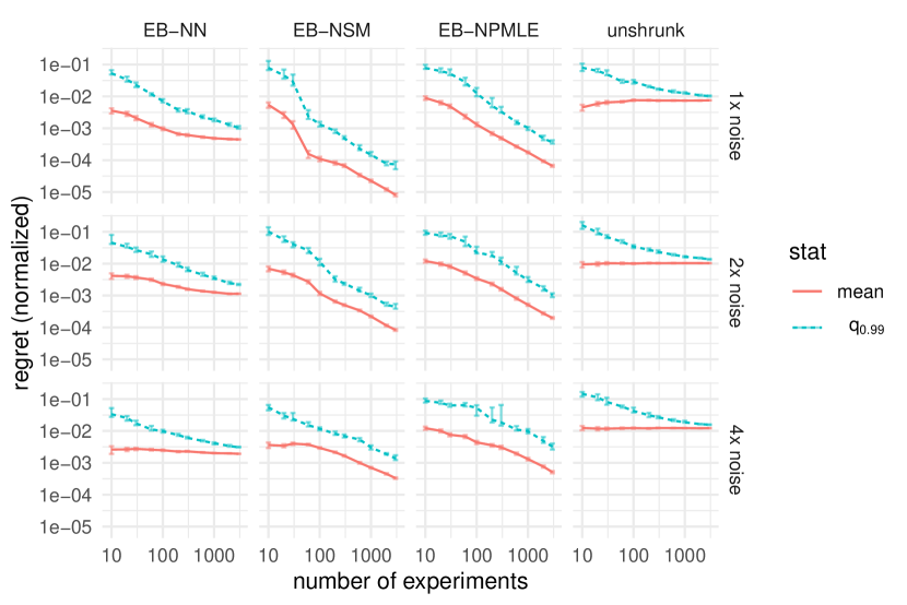
Figure 2: Regret $\mathcal{R}$ as the number of experiments $n$ increases, on a log scale and normalized by the standard deviation of the noise. Error bars around each point are the $95\%$ confidence intervals from uncertainty due to simulation error. For the choice sets based on the correctly specified EB-NSM and EB-NPMLE models, both the $99$th percentile and the mean show a trend of $\mathcal{O}(n^{-1})$. Regret does not appear to converge to zero for choice sets based on EB-NN (the normal-normal posterior mean estimator) or the naive choice set without shrinkage.

We compute other quantities of interest from (10), such as the proportion of mistakes in Figure 3 and the maximum magnitude of shrinkage error in Figure 4, as well as the $1$-Wasserstein distance of the true prior and the estimated prior in Figure 5. As expected, we see that the proportion of mistakes, their magnitude, and the 1-Wasserstein distance between the true and estimated prior in the correctly specified EB-NSM model all converge to zero at $n^{-1/2}$. The misspecified EB-NN model and the unshrunk procedure perform poorly in comparison, with the proportion and magnitude of mistakes not converging to zero, or even increasing, with the number of experiments. The most flexible model, EB-NPMLE, performs worse along every dimension than the more parsimonious EB-NSM, although the proportion and magnitude of mistakes it makes do both converge to zero.

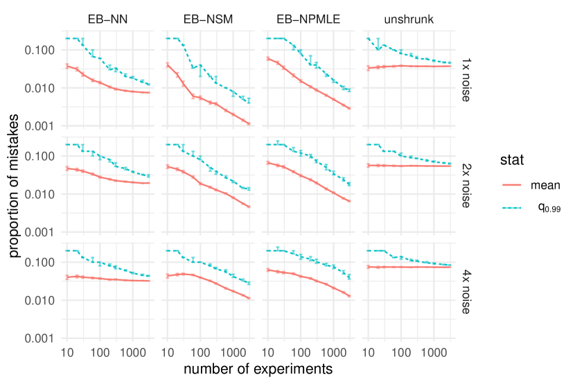
Figure 3: Proportion of mistakes as $n$ increases, on log scale. Error bars around each point are the $95\%$ confidence intervals from uncertainty due to simulation error. For the correctly specified $J_{\text{EB-NSM}}$, both the $99$th percentile and the mean show a trend of $\mathcal{O}(n^{-1/2})$. The highly flexible NPMLE shows a similar trend but generally makes more mistakes. The proportion does not appear to decrease towards zero for $J_{\text{EB-NN}}$ or $J_{\text{UN}}$.

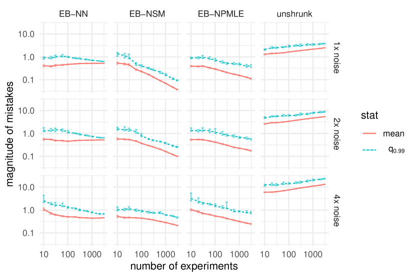
Figure 4: Maximum magnitude of shrinkage error as $n$ increases, on a log scale and normalized by the standard deviation of the noise. Error bars around each point are the $95\%$ confidence intervals from uncertainty due to simulation error. For the correctly specified $J_{\text{EB-NSM}}$, both the $99$th percentile and the mean show a trend of $\mathcal{O}(n^{-1/2})$ in the lower noise settings. The maximum magnitude does not appear to decrease indefinitely for $J_{\text{EB-NN}}$ or $J_{\text{UN}}$.

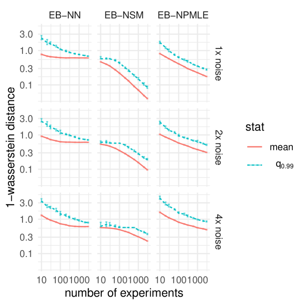
Figure 5: The $1$-Wasserstein distance between the true prior and the estimated prior, as $n$ increases, on a log scale and normalized by the standard deviation of the noise. Error bars around each point are the $95\%$ confidence intervals from uncertainty due to simulation error. As $n$ gets large, both the $99$th percentile and the mean show a trend of $\mathcal{O}(n^{-1/2})$ for EB-NSM. The distance eventually levels off away from zero for EB-NN because of misspecification. The distance for EB-NPMLE decreases but at a slower rate than $\mathcal{O}(n^{-1/2})$.

4 Conclusion

Our paper shows that empirical Bayes methods perform well in maximizing the aggregate value of the selected units, in the sense that the regret they incur converges to zero faster than the estimation error in the actual values themselves. This stands in contrast to prior work emphasizing the difficulty of accurately selecting the best units when the decision-maker incurs a constant loss from each misclassification (e.g. [45, 44, 29]). This underscores that rather than being inherent, the difficulty of the selection problem may depend critically on whether misclassification errors should be weighted by their severity in the utility function. Finally, we note that many extensions and variations on this setting are yet to be fully explored, including constructing confidence intervals for regret; characterizing the performance of decision rules for the frequentist analog of the Bayesian regret we study, treating the true values of units as non-stochastic; improving performance by incorporating unit-specific covariates into the analysis; tailoring the estimation of the prior to the specific selection problem at hand; and extending to an empirical Bayes knapsack problem where the selected items incur heterogeneous costs.

As discussed in Section 1, the frequentist optimal solution requires unavailable oracle knowledge of the e.c.d.f. of $\mu_{i}$’s. This implies that the empirical Bayes solution is not optimal in a minimax sense, with mainly two gaps: 1 the optimal solution in [59] is the Bayesian solution with a uniform prior on the permutations of $\mu_{i}$’s; 2 the loss in [59] is averaged over the e.c.d.f. instead of the uniform prior on permutations.

We suspect these gaps are small. [59] further conjectures that the Bayesian solution using the e.c.d.f. of $\mu_{i}$’s is asymptotically optimally; and when the class of prior $G(\cdot)$ is sufficiently large, this e.c.d.f. can be reasonably recovered as $G(\widehat{\eta})$. This suggests that both the solution and loss function are similar between the frequentist and the empirical Bayes setting, and hints at some loose optimality of the empirical Bayes approach. We hope this provides insights for appropriate convergence rates, analogous to those in [34, 28].

Appendix A Supporting Proofs

Claim 5.

For any exponential family $G(\eta)$ with finite variance, the mapping $\eta\mapsto G(\eta)$ is locally Lipschitz with respect to the $L_{1}$-norm (or equivalently any $L_{p}$-norm) in the domain and the $1$-Wasserstein distance in the codomain.

Proof.

Suppose the exponential family is given by

$$\exp(\eta^{\prime}T(x)-A(\eta))h(x)\,d\mu(x)$$

with $X$ as the variable and $T=T(X)$ as the canonical statistic. We wish to show that $|\int f(x)\,dG(\eta_{1})-\int f(x)\,dG(\eta_{0})|/\|\eta_{1}-\eta_{0}\|_{1}$ bounded for $\eta_{0}\neq\eta_{1}$, locally in $\eta$ and uniformly over all functions $f$ with Lipschitz constant $1$. By mean value theorem,

$$\left|\int f(x)\,dG(\eta_{1})-\int f(x)\,dG(\eta_{0})\right| =\left|(\eta_{1}-\eta_{0})^{\prime}\left.\nabla_{\eta}\int f(x)\,dG(\eta)\right|_{\eta=\eta^{\prime}}\right|$$

$$\leq\|\eta_{1}-\eta_{0}\|_{1}\left\|\left.\nabla_{\eta}\int f(x)\,dG(\eta)\right|_{\eta=\eta^{\prime}}\right\|_{\infty}.$$

for some $\eta^{\prime}$ that is also local. By [40, Theorem 2.4],

$$\nabla_{\eta}\int f(x)\,dG(\eta)=\int f(x)(T(x)-A^{\prime}(\eta))\,dG(\eta)=\operatorname{cov}_{\eta}(f(X),T(X)).$$

For $i$-th component of the covariance vector, we have

$$|\operatorname{cov}_{\eta}(f(X),T(X))_{i}|=|\operatorname{cov}_{\eta}(f(X),T_{i}(X))|\leq\sqrt{\operatorname{var}_{\eta}f(X)\operatorname{var}_{\eta}T_{i}(X)}.$$

$\operatorname{var}_{\eta}T_{i}(X)$ is given by $A^{\prime\prime}(\eta)_{ii}$, which is continuous by [5, Theorem 2.2] and thus locally bounded in $\eta$. For $\operatorname{var}_{\eta}f(X)$, suppose $X^{\prime}$ is an i.i.d. copy of $X$, then

$$\operatorname{var}_{\eta}f(X) =\frac{1}{2}(\operatorname{var}_{\eta}f(X)+\operatorname{var}_{\eta}f(X^{\prime}))$$

$$=\frac{1}{2}\operatorname{var}_{\eta}[f(X)-\mathbb{E}_{\eta}f(X)+\mathbb{E}_{\eta}f(X^{\prime})-f(X^{\prime})]$$

$$=\operatorname{var}_{\eta}[f(X)-f(X^{\prime})]$$

$$\leq\operatorname{var}_{\eta}(X-X^{\prime})$$

$$\leq\operatorname{var}_{\eta}X,$$

which is also continuous and thus locally bounded in $\eta$. ∎

Lemma 6.

Under Assumption 2, the posterior mean function $f_{\eta,\sigma}$ is strictly increasing and differentiable in $X$, and thus admits an inverse $f_{\eta,\sigma}^{-1}$ over its image.

Proof.

From [19], under $\mu\sim G(\eta)$ and $X\mid\mu\sim\mathcal{N}(\mu,\sigma^{2})$, we have $\nabla_{x}f_{\eta,\sigma}(x)=\sigma^{-2}\operatorname{var}(\mu\mid X=x)>0$. ∎

Lemma 7.

With Assumption 2, the c.d.f. $P$ of $\theta_{i}$ is continuously differentiable with positive derivative, or equivalently, $\theta_{i}$ has positive continuous density.

Proof.

The characteristic function of $X\mid\sigma$ is given by $\varphi_{G}(t)\exp(-\sigma^{2}t^{2}/2)$, where $\varphi_{G}$ is the characteristic function of $G$. Since $|\varphi_{G}(t)\exp(-\sigma^{2}t^{2}/2)|\leq\exp(-\sigma^{2}t^{2}/2)$ which is integrable, $X\mid\sigma$ has bounded continuous density [18, Theorem 3.3.14]. In fact the density is given by

$$p(X\mid\sigma)=\frac{1}{2\pi}\int e^{-itX}\varphi_{G}(t)\exp(-\sigma^{2}t^{2}/2)\,dt.$$

Since $\sigma$ is bounded away from $0$, dominated convergence theorem implies joint continuity of the density above in $(\sigma,X)$. In fact, by dominated convergence theorem and the fact that $t^{k}\exp(-\sigma^{2}t^{2}/2)$ is integrable for all integer $k\geq 0$, we can see that all higher derivatives of the density with respect to $X$ are continuous in $(\sigma,X)$.

Consider the mapping $X\mapsto\theta=f_{\eta_{0},\sigma}(X)$. By Lemma 6 it has a strictly positive derivative. Furthermore, since the derivative can be written in terms of the derivatives of $p(X\mid\sigma)$ [19], it is also continuous in $(\sigma,X)$. In other words, the density $p(\theta\mid\sigma)$ is continuous in $(\sigma,X)$.

Assumption 2 assumes the support of $\sigma$ is compact, so the density $p(\theta\mid\sigma)$ is naturally pointwise equicontinuous when viewed as a family of functions indexed by $\sigma$. Now for any $\theta$ and any $\varepsilon>0$, we can select $\delta>0$ such that for all $\sigma$ and all $\theta^{\prime}$ with $|\theta^{\prime}-\theta|<\delta$, we have $|p(\theta^{\prime}\mid\sigma)-p(\theta\mid\sigma)|<\varepsilon$ and so

$$\left|\int p(\theta^{\prime}\mid\sigma)\,dH_{0}-\int p(\theta\mid\sigma)\,dH_{0}\right|\leq\int|p(\theta^{\prime}\mid\sigma)-p(\theta\mid\sigma)|\,dH_{0}<\varepsilon,$$

and the marginal density of $\theta$ is continuous. ∎

Lemma 8.

Let $A$ be a metric space. Suppose $f(a,x)$ as a function from $A\times\mathbb{R}$ to $\mathbb{R}$ is continuous and has an inverse with respect to $x$, i.e. for all $a$ there exists $f^{-1}_{a}(\cdot)$ such that $f^{-1}_{a}\circ f(a,\cdot)=\text{id}_{\mathbb{R}}$. Then $(a,y)\mapsto f_{a}^{-1}(y)$ is also continuous.

Proof.

Let $(a_{n},y_{n})\to(a^{*},y^{*})$. It suffices to show that $f_{a_{n}}^{-1}(y_{n})\to f_{a^{*}}^{-1}(y^{*})$.

We first show that the sequence $x_{n}=f_{a_{n}}^{-1}(y_{n})$ is bounded. The sequence $y_{n}$ is bounded, so it is contained in some interval $(c+\varepsilon,d-\varepsilon)$ for some fixed $\varepsilon>0$ and $c,d$. By continuity of $f$, for $a$ sufficiently close to $a^{*}$, we have $f(a,f_{a^{*}}^{-1}(c))$ must be within $\varepsilon$ of $f(a^{*},f_{a^{*}}^{-1}(c))=c$. Similarly, $f(a,f_{a^{*}}^{-1}(d))$ can be within $\varepsilon$ of $d$. Since $f_{a}^{-1}$ is the inverse of a continuous function, it is monotonic. For $a$ sufficiently close to $a^{*}$,

$$~{}\{y_{n}\}\text{ is bounded by }c+\varepsilon\text{ and }d-\varepsilon$$

$$\Leftrightarrow ~{}\{f(a,f_{a}^{-1}(y_{n}))\}\text{ is bounded by }c+\varepsilon\text{ and }d-\varepsilon$$

$$\Rightarrow ~{}\{f(a,f_{a}^{-1}(y_{n}))\}\text{ is bounded by }f(a,f_{a^{*}}^{-1}(c))\text{ and }f(a,f_{a^{*}}^{-1}(d))$$

$$\Leftrightarrow ~{}\{f_{a}^{-1}(y_{n})\}\text{ is bounded by }f_{a^{*}}^{-1}(c)\text{ and }f_{a^{*}}^{-1}(d)$$

So for sufficiently large $n$, $a_{n}$ is sufficiently close to $a^{*}$, and $f_{a_{n}}^{-1}(y_{n})$ is bounded.

Since the sequence $x_{n}=f_{a_{n}}^{-1}(y_{n})$ is bounded, it must have a convergent subsequence. Consider any of such convergent subsequence indexed by $n_{k}$. We have

$$f(a^{*},\lim_{k\to\infty}x_{n_{k}}) =f(\lim_{k\to\infty}a_{n_{k}},x_{n_{k}})$$

$$=\lim_{k\to\infty}f(a_{n_{k}},x_{n_{k}})$$

$$=\lim_{k\to\infty}f(a_{n_{k}},f_{a_{n}}^{-1}(y_{n}))$$

$$=y^{*}$$

$$=f(a^{*},f_{a^{*}}^{-1}(y^{*})),$$

and thus $\lim_{k\to\infty}x_{n_{k}}=f_{a^{*}}^{-1}(y^{*})$. Since $f_{a_{n}}^{-1}(y_{n})$ is bounded and any of its convergent subsequence converges to the same limit $f_{a^{*}}^{-1}(y^{*})$, it also converges to the same limit, completing the proof of continuity. ∎

Lemma 9.

If for any non-decreasing divergent sequence of real numbers $(a_{n})_{n\in\mathbb{N}}$ the sequence of random variables $(X_{n})_{n\in\mathbb{N}}$ is $\mathcal{O}_{p}(a_{n})$, then it is also $\mathcal{O}_{p}(1)$.

Proof.

Suppose $X_{n}\neq\mathcal{O}_{p}(1)$. Then there exists $\varepsilon>0$ such that for all $M>0$, there are infinitely many $n$ such that

$$\mathbb{P}(|X_{n}|>M)\geq\varepsilon.$$ (16)

Take $n_{1}$ to be the smallest $n$ satisfying (16) with $M=1$. For $i>1$, take $n_{i}$ to be the smallest $n>n_{i-1}$ satisfying (16) with $M=i^{2}$. Specifically, $(n_{i})_{i\in\mathbb{N}}$ is a strictly increasing sequence such that

$$\mathbb{P}(|X_{n_{i}}|>i^{2})\geq\varepsilon\quad\text{for all $i$.}$$

Now we are ready to set up a sequence that grows sufficiently slowly to cause a contradiction. For any $n$, take $b_{n}=i$ where $n\in[n_{i},n_{i+1})$. Since $(n_{i})_{i\in\mathbb{N}}$ is strictly increasing and only takes values in integers, $(b_{n})_{i\in\mathbb{N}}$ is a non-decreasing sequence with $\lim_{n\to\infty}b_{n}=\infty$. So $X_{n}=\mathcal{O}_{p}(b_{n})$ and there exists $M^{\prime},N^{\prime}$ such that

$$\mathbb{P}(|X_{n}|/b_{n}>M^{\prime})<\varepsilon\quad\text{for all $n>N^{\prime}$.}$$

So for sufficiently large $i>M^{\prime}$,

$$\varepsilon>\mathbb{P}(|X_{n_{i}}|/b_{n_{i}}>M^{\prime})=\mathbb{P}(|X_{n_{i}}|>M^{\prime}i)\geq\mathbb{P}(|X_{n_{i}}|>i^{2})\geq\varepsilon,$$

leading to a contradiction. ∎

References

- [1] Isaiah Andrews, Toru Kitagawa, and Adam McCloskey. Inference on winners. Technical report, National Bureau of Economic Research, 2019.
- [2] Eduardo M Azevedo, Alex Deng, José L Montiel Olea, and E Glen Weyl. Empirical bayes estimation of treatment effects with many a/b tests: An overview. In AEA Papers and Proceedings, volume 109, pages 43–47, 2019.
- [3] Eduardo M Azevedo, Alex Deng, José Luis Montiel Olea, Justin Rao, and E Glen Weyl. A/b testing with fat tails. Journal of Political Economy, 128(12):4614–000, 2020.
- [4] Peter Bergman, Raj Chetty, Stefanie DeLuca, Nathaniel Hendren, Lawrence F Katz, and Christopher Palmer. Creating moves to opportunity: Experimental evidence on barriers to neighborhood choice. Technical report, National Bureau of Economic Research, 2019.
- [5] Lawrence D. Brown. Fundamentals of statistical exponential families with applications in statistical decision theory. Institute of Mathematical Statistics, 1986.
- [6] Lawrence D Brown. In-season prediction of batting averages: A field test of empirical bayes and bayes methodologies. The Annals of Applied Statistics, 2(1):113–152, 2008.
- [7] Raymond J Carroll and Peter Hall. Optimal rates of convergence for deconvolving a density. Journal of the American Statistical Association, 83(404):1184–1186, 1988.
- [8] Jiahua Chen. Optimal rate of convergence for finite mixture models. The Annals of Statistics, pages 221–233, 1995.
- [9] Lijie Chen, Jian Li, and Mingda Qiao. Nearly Instance Optimal Sample Complexity Bounds for Top-k Arm Selection. In Aarti Singh and Jerry Zhu, editors, Proceedings of the 20th International Conference on Artificial Intelligence and Statistics, volume 54 of Proceedings of Machine Learning Research, pages 101–110. PMLR, 20–22 Apr 2017.
- [10] Raj Chetty, John N Friedman, and Jonah E Rockoff. Measuring the impacts of teachers I: Evaluating bias in teacher value-added estimates. American economic review, 104(9):2593–2632, 2014.
- [11] Raj Chetty, John N Friedman, and Jonah E Rockoff. Measuring the impacts of teachers II: Teacher value-added and student outcomes in adulthood. American economic review, 104(9):2633–79, 2014.
- [12] Dominic Coey and Tom Cunningham. Improving treatment effect estimators through experiment splitting. In The World Wide Web Conference, pages 285–295, 2019.
- [13] Arthur Cohen and Harold B. Sackrowitz. Two stage conditionally unbiased estimators of the selected mean. Statistics & Probability Letters, 8(3):273–278, 1989.
- [14] Ram C. Dahiya. Estimation of the mean of the selected population. Journal of the American Statistical Association, 69(345):226–230, 1974.
- [15] Alex Deng. Objective bayesian two sample hypothesis testing for online controlled experiments. In Proceedings of the 24th International Conference on World Wide Web, pages 923–928, 2015.
- [16] Alex Deng, Yicheng Li, Jiannan Lu, and Vivek Ramamurthy. On post-selection inference in a/b testing. In Proceedings of the 27th ACM SIGKDD Conference on Knowledge Discovery & Data Mining, KDD ’21, page 2743–2752, New York, NY, USA, 2021. Association for Computing Machinery.
- [17] Justin B Dimick, Douglas O Staiger, and John D Birkmeyer. Ranking hospitals on surgical mortality: the importance of reliability adjustment. Health services research, 45(6p1):1614–1629, 2010.
- [18] Rick Durrett. Probability: Theory and examples. Cambridge University Press, 2009.
- [19] Bradley Efron. Tweedie’s formula and selection bias. Journal of the American Statistical Association, 106(496):1602–1614, 2011.
- [20] Bradley Efron. Two modeling strategies for empirical bayes estimation. Statistical science: a review journal of the Institute of Mathematical Statistics, 29(2):285, 2014.
- [21] Bradley Efron and Carl Morris. Stein’s estimation rule and its competitors—an empirical bayes approach. Journal of the American Statistical Association, 68(341):117–130, 1973.
- [22] Bradley Efron and Carl Morris. Stein’s paradox in statistics. Scientific American, 236(5):119–127, 1977.
- [23] Bradley Efron and Robert Tibshirani. Empirical bayes methods and false discovery rates for microarrays. Genetic epidemiology, 23(1):70–86, 2002.
- [24] William Fithian, Dennis Sun, and Jonathan Taylor. Optimal inference after model selection. arXiv preprint arXiv:1410.2597, 2014.
- [25] Michael Gilraine, Jiaying Gu, and Robert McMillan. A new method for estimating teacher value-added. Technical report, National Bureau of Economic Research, 2020.
- [26] David Goldberg and James E Johndrow. A decision theoretic approach to a/b testing. arXiv preprint arXiv:1710.03410, 2017.
- [27] Harvey Goldstein and David J Spiegelhalter. League tables and their limitations: statistical issues in comparisons of institutional performance. Journal of the Royal Statistical Society: Series A (Statistics in Society), 159(3):385–409, 1996.
- [28] Eitan Greenshtein and Ya’acov Ritov. Asymptotic Efficiency of Simple Decisions for the Compound Decision Problem. In Institute of Mathematical Statistics Lecture Notes - Monograph Series, pages 266–275. Institute of Mathematical Statistics, Beachwood, Ohio, USA, 2009.
- [29] Jiaying Gu and Roger Koenker. Invidious comparisons: Ranking and selection as compound decisions. arXiv preprint arXiv:2012.12550, 2020.
- [30] F Richard Guo, James McQueen, and Thomas S Richardson. Empirical bayes for large-scale randomized experiments: a spectral approach. arXiv preprint arXiv:2002.02564, 2020.
- [31] Xinzhou Guo and Xuming He. Inference on selected subgroups in clinical trials. Journal of the American Statistical Association, 116(535):1498–1506, 2021.
- [32] Shanti S Gupta and Jianjun Li. On empirical bayes procedures for selecting good populations in a positive exponential family. Journal of Statistical planning and Inference, 129(1-2):3–18, 2005.
- [33] Shanti S Gupta and Subramanian Panchapakesan. Multiple decision procedures: theory and methodology of selecting and ranking populations. SIAM, 2002.
- [34] James F Hannan and JR Van Ryzin. Rate of convergence in the compound decision problem for two completely specified distributions. The Annals of Mathematical Statistics, pages 1743–1752, 1965.
- [35] Douglas N Harris and Tim R Sass. Skills, productivity and the evaluation of teacher performance. Economics of Education Review, 40:183–204, 2014.
- [36] Peter Hull. Estimating hospital quality with quasi-experimental data. Available at SSRN 3118358, 2018.
- [37] Kenneth Hung and William Fithian. Rank verification for exponential families. The Annals of Statistics, 47(2):758 – 782, 2019.
- [38] Brian A Jacob and Lars Lefgren. Can principals identify effective teachers? evidence on subjective performance evaluation in education. Journal of labor Economics, 26(1):101–136, 2008.
- [39] Thomas J Kane, Jonah E Rockoff, and Douglas O Staiger. What does certification tell us about teacher effectiveness? evidence from new york city. Economics of Education review, 27(6):615–631, 2008.
- [40] Robert W Keener. Theoretical statistics: Topics for a core course. Springer, 2010.
- [41] Jack Kiefer and Jacob Wolfowitz. Consistency of the maximum likelihood estimator in the presence of infinitely many incidental parameters. The Annals of Mathematical Statistics, pages 887–906, 1956.
- [42] Patrick Kline and Christopher Walters. Reasonable doubt: Experimental detection of job-level employment discrimination. Econometrica, 89(2):765–792, 2021.
- [43] Roger Koenker and Ivan Mizera. Convex optimization, shape constraints, compound decisions, and empirical bayes rules. Journal of the American Statistical Association, 109(506):674–685, 2014.
- [44] Rongheng Lin, Thomas A Louis, Susan M Paddock, and Greg Ridgeway. Loss function based ranking in two-stage, hierarchical models. Bayesian Analysis, 1(4):915, 2006.
- [45] JR Lockwood, Thomas A Louis, and Daniel F McCaffrey. Uncertainty in rank estimation: Implications for value-added modeling accountability systems. Journal of educational and behavioral statistics, 27(3):255–270, 2002.
- [46] Roger J Marshall. Mapping disease and mortality rates using empirical bayes estimators. Journal of the Royal Statistical Society: Series C (Applied Statistics), 40(2):283–294, 1991.
- [47] J. Nathan Matias, Kevin Munger, Marianne Aubin Le Quere, and Charles Ebersole. The upworthy research archive, a time series of 32,487 experiments in u.s. media. Scientific Data, 8(1):195, 2021.
- [48] M Mogstad, J Romano, A Shaikh, and D Wilhelm. Comment on” invidious comparisons: Ranking and selection as compound decisions”. Econometrica, 2022.
- [49] Magne Mogstad, Joseph P Romano, Azeem Shaikh, and Daniel Wilhelm. Inference for ranks with applications to mobility across neighborhoods and academic achievement across countries. Technical report, National Bureau of Economic Research, 2020.
- [50] Yury Polyanskiy and Yihong Wu. Sharp regret bounds for empirical bayes and compound decision problems. arXiv preprint arXiv:2109.03943, 2021.
- [51] Herbert Robbins. An empirical bayes approach to statistics. In Proceedings of the Third Berkeley Symposium on Mathematical Statistics and Probability, Volume 1: Contributions to the Theory of Statistics, pages 157–163. University of California Press, 1956.
- [52] Herbert Robbins. The empirical bayes approach to statistical decision problems. The Annals of Mathematical Statistics, 35(1):1–20, 1964.
- [53] Xuedong Shang, Rianne de Heide, Pierre Menard, Emilie Kaufmann, and Michal Valko. Fixed-confidence guarantees for bayesian best-arm identification. In Silvia Chiappa and Roberto Calandra, editors, Proceedings of the Twenty Third International Conference on Artificial Intelligence and Statistics, volume 108 of Proceedings of Machine Learning Research, pages 1823–1832. PMLR, 26–28 Aug 2020.
- [54] Gordon K Smyth. Linear models and empirical bayes methods for assessing differential expression in microarray experiments. Statistical applications in genetics and molecular biology, 3(1), 2004.
- [55] Matthew Stephens. False discovery rates: a new deal. Biostatistics, 18(2):275–294, 10 2016.
- [56] Neal Thomas, Nicholas T Longford, and John E Rolph. Empirical bayes methods for estimating hospital-specific mortality rates. Statistics in medicine, 13(9):889–903, 1994.
- [57] Aad W van der Vaart. Asymptotic statistics, volume 3. Cambridge university press, 2000.
- [58] John Van Ryzin and Vyaghreswarudu Susarla. On the empirical bayes approach to multiple decision problems. The Annals of Statistics, 5(1):172–181, 1977.
- [59] Asaf Weinstein. On permutation invariant problems in large-scale inference. arXiv preprint arXiv:2110.06250, 2021.
- [60] Asaf Weinstein, Zhuang Ma, Lawrence D. Brown, and Cun-Hui Zhang. Group-linear empirical bayes estimates for a heteroscedastic normal mean. Journal of the American Statistical Association, 113(522):698–710, 2018.
- [61] Jason Willwerscheid and Matthew Stephens. ebnm: An R package for solving the empirical bayes normal means problem using a variety of prior families. arXiv, 2021.
- [62] Peng Yu, Spencer S Ericksen, Anthony Gitter, and Michael A Newton. Bayes optimal informer sets for early-stage drug discovery. arXiv preprint arXiv:2011.06122, 2020.
- [63] Cun-Hui Zhang. Empirical bayes and compound estimation of normal means. Statistica Sinica, 7(1):181–193, 1997.