Constraining ultralight vector dark matter with the Parkes Pulsar Timing Array second data release

Abstract

Composed of ultralight bosons, fuzzy dark matter provides an intriguing solution to challenges that the standard cold dark matter model encounters on sub-galactic scales. The ultralight dark matter with mass $m\sim 10^{-23}\rm{eV}$ will induce a periodic oscillation in gravitational potentials with a frequency in the nanohertz band, leading to observable effects in the arrival times of radio pulses from pulsars. Unlike scalar dark matter, pulsar timing signals induced by the vector dark matter are dependent on the oscillation direction of the vector fields. In this work, we search for ultralight vector dark matter in the mass range of $[2\times 10^{-24},2\times 10^{-22}\,\mathrm{]}{\rm{eV}}$ through its gravitational effect in the Parkes Pulsar Timing Array (PPTA) second data release. Since no statistically significant detection is made, we place $95\%$ upper limits on the local dark matter density as $\rho_{\rm{\tiny{VF}}}\lesssim 5\,\mathrm{\rm{GeV/cm^{3}}}$ for $m\lesssim 10^{-23}\,\mathrm{\rm{eV}}$. As no preferred direction is found for the vector dark matter, these constraints are comparable to those given by the scalar dark matter search with an earlier 12-year data set of PPTA.

I Introduction

Numerous astrophysical observations, such as galaxy rotational curves Rubin et al. (1980, 1982), velocity dispersions (Faber and Jackson, 1976), and gravitational lensing (Massey et al., 2010) reveal the existence of invisible matter, the so-called dark matter. In combination with observational evidence of the Universe’s accelerating expansion, the standard Lambda Cold Dark Matter ($\rm{\Lambda}$CDM) cosmological model has been established. Precision analyses of the cosmic microwave background show that dark matter constitutes $26\%$ of the total energy density of the present-day universe (Aghanim et al., 2020).

The cold dark matter paradigm has achieved great success in describing the structure of galaxies on large scales (Roszkowski et al., 2018; Marsh, 2016; Wantz and Shellard, 2010), but it is met with puzzling discrepancies between the predictions and observations of galaxies and their clustering on small scales. For example, the N-body simulations based on the cold dark matter model show a much steeper central density profile in the dark matter halos than that inferred from the galaxy rotational curves (the “core-cusp problem” Gentile et al. (2004); de Blok (2010)). The predicted number of subhalos with decreasing mass grows much more steeply than what is observed around galaxies (the “missing-satellites problem” Moore et al. (1999); Klypin et al. (1999)).

Because of the difficulty in solving the small-scale problems as well as the null result in searching for traditional cold dark matter candidates, e.g., weakly interactive massive particles (Schumann, 2019), alternative paradigms for dark matter have been proposed. These include the warm dark matter (Bode et al., 2001) and fuzzy dark matter (Hu et al., 2000).

The term “fuzzy dark matter” often refers to ultralight scalar particles with a mass around $m\sim 10^{-22}\,\mathrm{\rm eV}$. Such a dark matter scenario can get the correct relic abundance through the misalignment mechanism similar to that of axions (Fox et al., 2004); that is, when the initial value of the scalar field is away from its potential minimum, the field is condensed during inflation when its mass is smaller than the Hubble scale, and then starts a coherent oscillation as a non-relativistic matter at a later epoch. Fuzzy dark matter makes the same large-scale structure predictions as $\rm{\Lambda}$CDM, but the particle’s large de Broglie wavelength, $\lambda\sim\rm{kpc}$, suppresses the structure on small scales and thus explains well the corresponding smaller-scale observational phenomena (Hui et al., 2017).

Besides the scalar particle, a naturally light vector boson predicted in string-inspired models with compactified extra dimensions (Goodsell et al., 2009) can also act as a good fuzzy dark matter candidate. There are several mechanisms to produce vector dark matter with the correct relic abundance, such as the misalignment mechanism (Nelson and Scholtz, 2011; Nakayama, 2019), quantum fluctuations during inflation (Graham et al., 2016a; Nomura et al., 2020), and decay of a network of global cosmic strings (Long and Wang, 2019). Because of their different spins, if the dark matter is assumed to have interaction with Standard Model, scalar and vector fields couple with Standard Model particles in ways which lead to different observable phenomena. For example, if the vector dark matter particle is a $U(1)_{B}$ (“$B$” refers to baryon ) or $U(1)_{B-L}$ (“$L$” refers to lepton) gauge boson, the so-called “dark photon” would interact with ordinary matter (Graham et al., 2016b), then it can be detected with gravitational-wave interferometers because it exerts forces on test masses and results in displacements (Pierce et al., 2018; Abbott et al., 2022); it can also be detected with binary pulsar systems via its effects on the secular dynamics of binary systems (Blas et al., 2017; López Nacir and Urban, 2018). Such a gauge effect is not applicable to scalar dark matter (Antypas et al., 2022).

In addition to unknown interaction with the Standard Model, pure gravitational effects of fuzzy dark matter can also lead to observable results and help distinguish the scalar and vector dark matter. The dark matter field with ultralight mass has a wave nature with the oscillating frequency of $f_{\rm{dm}}=mc^{2}/h=2.4\times 10^{-9}(mc^{2}/10^{-23}\rm{eV})\,\mathrm{{Hz}}$. Such a coherently oscillating field leads to periodic oscillations in the gravitational potentials and further induces periodic signals with the frequency on the order of nanohertz (Khmelnitsky and Rubakov, 2014; Nomura et al., 2020), which falls into the sensitive range of the pulsar timing arrays (PTAs). A PTA consists of stable millisecond pulsars for which times of arrival (ToAs) of radio pulses are monitored with high precision over a course of years to decades (Sazhin, 1978; Detweiler, 1979; Foster and Backer, 1990). Any unmodelled signal will induce timing residues, which represent the difference between the measured and predicted ToAs.

In contrast to the ultralight scalar dark matter, the timing residuals caused by the ultralight vector dark matter are dependent on the oscillation direction of the vector fields (Khmelnitsky and Rubakov, 2014; Nomura et al., 2020). Several previous works have used PTA data to search for ultralight scalar dark matter (Porayko and Postnov, 2014; Porayko et al., 2018; Kato and Soda, 2020). In a recent work Xue et al. (2022), a search was performed for the dark photon dark matter in the PPTA second data release (DR2) based on the gauge effect. This resulted in upper limits on the coupling strength between dark photons and ordinary matter, assuming that all dark matter is composed of ultralight dark photons. In this work, we search for ultralight vector dark matter in the mass range of $[2\times 10^{-24},2\times 10^{-22}\,\mathrm{]}{\rm{eV}}$ in the PPTA DR2 data set based on the gravitational effect without assuming its interaction with Standard Model particles.

This paper is organized as follows. In Sec. II we describe the observable pulsar timing effects induced by vector dark matter. In Sec. III we provide details of our data analysis. We present the results and conclusions in Sec. IV. In the following sections, we set $c=\hbar=1$.

II Gravitational Effect from vector dark matter

In this section, we first introduce the timing residuals caused by the gravitational effect from the ultralight vector dark matter in the Galaxy; a more detailed derivation can be found in Ref. (Nomura et al., 2020).

Assuming no coupling between the ultralight particles and any other fields, we take the action for a free vector field $A_{\mu}$ with mass $m$ as,

$$S=\int d^{4}x\sqrt{-g}\left(-\frac{1}{4}F^{\mu\nu}F_{\mu\nu}-\frac{1}{2}m^{2}A_{\mu}A^{\mu}\right),$$ (1)

where $g$ is the determinant of the metric $g_{\mu\nu}$ and $F_{\mu\nu}=\partial_{\mu}A_{\nu}-\partial_{\nu}A_{\mu}$. On Galactic scales, the cosmic expansion is negligible and the background is approximately Minkowski. The energy-momentum tensor carried by the vector dark matter induces perturbations into the metric which, in the Newtonian gauge, can be written as

$$\begin{split}ds^{2}=&\eta_{\mu\nu}dx^{\mu}dx^{\nu}-2\Phi(t,\mathbf{x})dt^{2}+2\Psi(t,\mathbf{x})\delta_{ij}dx^{i}dx^{j}\\ &+h_{ij}(t,\mathbf{x})dx^{i}dx^{j}\,,\end{split}$$ (2)

where $\eta_{\mu\nu}=\rm{diag}(-1,+1,+1,+1)$ is the background Minkowski metric, $\Phi$ and $\Psi$ are gravitational potentials, and $h_{ij}$ describes the traceless spatial metric perturbations. $h_{ij}$ is absent in the scalar-field case and demonstrates the anisotropy induced by additional degrees of freedom in vector fields.

With a huge occupation number, the vector field can be described as a classical wave with a monochromatic frequency determined by its mass. This is a good approximation because the characteristic speed of the dark matter is non-relativistic $v\sim 10^{-3}$. During inflation, only the longitudinal mode of the vector fields survives (Graham et al., 2016a), so the equation of motion of the vector field is given by the component in the oscillating direction $\hat{k}=(\sin\theta\cos\phi,\sin\theta\sin\phi,\cos\theta)$,

$$A_{\hat{k}}(t,\mathbf{x})=A(\mathbf{x})\cos(mt+\alpha(\mathbf{x})).$$ (3)

The vector fields contribute a time-independent energy density

$$\rho_{\rm{\tiny{VF}}}(x)=\frac{1}{2}m^{2}A^{2}(x),$$ (4)

and an anisotropic oscillating pressure which leads to oscillating gravitational potentials. By solving the photon geodesic equation from the pulsar to the Earth under the metric Eq. (2), it is found that the metric perturbations that give rise to the observable effects in PTAs are from the spatial components (see the Appendix of (Nomura et al., 2020)). Furthermore, splitting the potential $\Psi$ into a dominant time-independent part and an oscillating part and solving the linear Einstein equation by neglecting the spatial gradient of the oscillating part (which is suppressed by order of $v\sim 10^{-3}$), the spatial perturbations take the following form,

$$\!\!\!\!\Psi(t,\mathbf{x}) \!=\! \Psi_{0}(\mathbf{x})+\Psi_{\mathrm{osc}}(\mathbf{x})\cos(2mt+2\alpha(\mathbf{x})),$$ (5)

$$\!\!\!\!h_{ij}(t,\mathbf{x}) \!=\! h_{\mathrm{osc}}(\mathbf{x})\!\cos(2mt\!+\!2\alpha(\mathbf{x}))(\hat{l}\otimes\hat{l}\!+\!\hat{n}\otimes\hat{n}\!-\!2\hat{k}\otimes\hat{k}),$$ (6)

where $\Psi_{0}(x)$ is the potential independent of time determined by the local energy density of the vector field dark matter $\rho_{\rm{\tiny{VF}}}(x)$, and $\hat{l}$ and $\hat{n}$ are the unit vectors perpendicular to the propagation direction given by $\hat{l}=(\sin\phi,-\cos\phi,0)$ and $\hat{n}=(\cos\theta\cos\phi,\cos\theta\sin\phi,-\sin\theta)$, respectively. The amplitudes of potentials in the oscillation part can also be related to $\rho_{\rm{\tiny{VF}}}(x)$ through the relationship between $A(x)$ with $\rho_{\rm{\tiny{VF}}}(x)$ (Eq. (4)),

$$\Psi_{\mathrm{osc}}(\mathbf{x}) = -\frac{\pi G\rho_{\rm{\tiny{VF}}}(\mathbf{x})}{3m^{2}}$$ (7)

$$= -2.2\times 10^{-16}\frac{\rho_{\rm{\tiny{VF}}}(\mathbf{x})}{\rho_{0}}\left(\frac{10^{-23}\mathrm{eV}}{m}\right)^{2},$$

$$h_{\mathrm{osc}}(\mathbf{x}) = \frac{8\pi G\rho_{\rm{\tiny{VF}}}(\mathbf{x})}{3m^{2}}$$ (8)

$$= 1.7\times 10^{-15}\frac{\rho_{\rm{\tiny{VF}}}(\mathbf{x})}{\rho_{0}}\left(\frac{10^{-23}\mathrm{eV}}{m}\right)^{2}.$$

where we use the measured local energy density $\rho_{0}=0.4\,\mathrm{\mathrm{GeV}/\mathrm{cm}^{3}}$ (Salucci et al., 2010) as the normalized factor, and the oscillation frequency in potentials is given by:

$$f=\frac{2m}{2\pi}=4.8\times 10^{-9}\mathrm{~{}Hz}\left(\frac{m}{10^{-23}\mathrm{eV}}\right).$$ (9)

The oscillating part of spatial metric $\Psi$ and $h_{ij}$ induces a mearsurable redshift in the radio pulse propagating from a pulsar to the Earth

$$z_{\Psi}(t)= \Psi_{\mathrm{osc}}(\mathbf{x}_{e})\cos(2mt+2\alpha(\mathbf{x}_{e}))$$ (10)

$$-\Psi_{\rm{osc}}(\mathbf{x}_{p})\cos[2m(t-|\mathbf{x}_{p}|)+2\alpha(\mathbf{x}_{p})],$$

$$z_{h}(t)= \frac{1}{2}\hat{p}^{i}\hat{p}^{j}[h_{ij}(t,\mathbf{x}_{e})-h_{ij}(t-|\mathbf{x}_{p}|,\mathbf{x}_{p})],$$ (11)

where $\mathbf{x}_{e}$ and $\mathbf{x}_{p}$ respectively represent the location of the Earth and the pulsar, and $\hat{p}$ is the unit vector pointing to the pulsar. As the distance between most pulsars and the Earth is at the order of $\mathcal{O}(\mathrm{kpc})$, which is comparable to the de Broglie wavelength of the dark matter, it is legitimate to assume that they are in a region where the vector dark matter keeps its coherent oscillation direction, and that the Earth term and the pulsar term take the same amplitudes $\Psi_{\rm osc}$ and $h_{\rm osc}$.

Integrating the redshifts separately, the results combine into the total timing residuals,

$$R_{t}= R_{\Psi}+R_{h}$$

$$= \frac{h_{\rm osc}}{\pi f}\left\{\frac{1}{2}\left[(\hat{p}\cdot\hat{l})^{2}+(\hat{p}\cdot\hat{n})^{2}-2(\hat{p}\cdot\hat{k})^{2}\right]-\frac{1}{8}\right\}$$ (12)

$$\times\sin(\alpha_{e}-\alpha_{p})\cos\left(2\pi ft+\alpha_{e}+\alpha_{p}\right),$$

where we have defined the phases in Earth term and pulsar term as $\alpha_{e}=\alpha(\mathbf{x}_{e})$ and $\alpha_{p}=\alpha\left(\mathbf{x}_{p}\right)-m\left|\mathbf{x}_{p}\right|$, respectively. Eq. (12) shows that timing residuals induced by the coherent oscillation of vector dark matter is angle dependent, which is a distinctive feature in comparison to the scalar dark matter; see Ref. (Nomura et al., 2020) for a more detailed comparison.

III Data analysis

Now we turn to search for ultralight vector dark matter in the PPTA DR2 data set, which includes observations for 26 pulsars with a timespan up to 15 years. By balancing sensitivity and computational costs, we choose the six best pulsars, i.e., those with relatively long observational timespan and high timing precision in the array. A summary of the basic properties of these six pulsars is given in Table 1.

Table 1: Basic properties of the 6 pulsars used in our analysis. RMS – the weighted root-mean-square band-averaged post-fit timing residuals, $N_{\rm{obs}}$ – the number of observations, $N_{\rm{ToA}}$ – the number of ToAs, Span – observational data span. See Ref. (Kerr et al., 2020) for details.

Pulsar Name	RMS [$\mu$s]	$N_{\rm{obs}}$	$N_{\rm{ToA}}$	Span [$\mathrm{yr}$]
J0437$-$4715	0.59	4149	29262	15.0
J1600$-$3053	0.58	1096	7047	14.2
J1713+0747	0.32	1049	7804	14.2
J1744$-$1134	0.46	939	6717	14.2
J1909$-$3744	0.24	2223	14627	14.2
J2241$-$5236	0.26	821	5224	8.2

We process the data in the same way as Refs. Porayko et al. (2018); Xue et al. (2022). To extract the target signal from the ToAs, one needs to provide a comprehensive analysis on the noise that might be present in timing residuals. After subtracting the expected arrival times described by the timing model, the timing residuals can be decomposed into

$$\delta\bm{t}=M{\bm{\epsilon}}+\delta\bm{t}_{n}+\delta\bm{t}_{s},$$ (13)

where $M{\bm{\epsilon}}$ accounts for the inaccuracy of the timing model with $M$ being the design matrix and $\bm{\epsilon}$ being the vector of timing model parameter offsets, $\delta\bm{t}_{n}$ contains noise contributions, and $\delta\bm{t}_{s}$, given by Eq. (12), is the signal that we are searching for.

Table 2: Parameters and their prior distributions used in the analyses. Here U and log-U represent a uniform and log uniform distribution, respectively. Here “one parameter for PTA” means the parameter is common in the whole data set, while “one parameter per pulsar” indicates the parameter varies from pulsar to pulsar; the same goes for the case of “one parameter per band/system” and “one parameter per exponential-dip event”.

Parameter	description	prior	comments
White noise
$E_{k}$	EFAC per backend/receiver system	$\mathrm{U}[0,10]$	single-pulsar analysis only
$Q_{k}\,[\mathrm{s}]$	EQUAD per backend/receiver system	$\operatorname{\mathrm{log-U}}[-8.5,-5]$	single-pulsar analysis only
$J_{k}\,[\mathrm{s}]$	ECORR per backend/receiver system	$\operatorname{\mathrm{log-U}}[-8.5,-5]$	single-pulsar analysis only
Red noise (including SN and DM)
$\mathcal{A}_{\mathrm{RN}}$	Red-noise power-law amplitude	$\operatorname{\mathrm{log-U}}[-20,-8]$	one parameter per pulsar
$\gamma_{\mathrm{RN}}$	red-noise power-law index	$\mathrm{U}[0,10]$	one parameter per pulsar
Band/System noise
$\mathcal{A}_{\mathrm{BN},\mathrm{GN}}$	band/group-noise power-law amplitude	$\operatorname{\mathrm{log-U}}[-20,-8]$	one parameter per band/system
$\gamma_{\mathrm{BN},\mathrm{GN}}$	band/group-noise power-law index	$\mathrm{U}[0,10]$	one parameter per band/system
Deterministic event
$\mathcal{A}_{\mathrm{E}}$	exponential-dip amplitude	$\operatorname{\mathrm{log-U}}[-10,-2]$	one parameter per exponential-dip event
$t_{\mathrm{E}}\,[\mathrm{MJD}]$	time of the event	$\mathrm{U}[54500,54900]$ for PSR J1713	first exponential-dip event
		$\mathrm{U}[57500,57520]$ for PSR J1713	second exponential-dip event
$\mathrm{log_{10}}\tau_{\mathrm{E}}\,[\mathrm{MJD}]$	relaxation time for the dip	$\mathrm{U}[\mathrm{log_{10}}5,2]$	one parameter per exponential-dip event
Common noise
$\mathcal{A}_{\rm{CN}}$	common-noise power-law amplitude	$\operatorname{\mathrm{log-U}}[-18,-11]$	one parameter for PTA
$\gamma_{\rm{CN}}$	common noise power-law index	$\mathrm{U}[0,7]$	one parameter for PTA
Ultralight vector dark matter signal
$h_{\rm{osc}}$	oscillation amplitude	$\operatorname{\mathrm{log-U}}[-19,-10]$ (search)	one parameter for PTA
		$\mathrm{U}[-19,-10]$ (limit)
$\alpha_{e}$	oscillation phase on Earth	$\mathrm{U}[0,2\pi]$	one parameter for PTA
$\alpha_{p}$	equivalent oscillation phase on pulsar	$\mathrm{U}[0,2\pi]$	one parameter per pulsar
$\cos\theta$	polar angle of propagation direction	$\mathrm{U}[-1,1]$	one parameter for PTA
$\phi$	azimuth angle of propagation direction	$\mathrm{U}[0,2\pi]$	one parameter for PTA
$f\,[\mathrm{Hz}]$	oscillation frequency	$\operatorname{\mathrm{log-U}}[-9,-7]$ (search)	one parameter for PTA
		delta function (limit)	fixed
BayesEphem
$z_{\mathrm{drift}}$	drift-rate of Earth’s orbit about ecliptic z-axis	$\mathrm{U}[-10^{-9},10^{-9}]$	one parameter for PTA
$\Delta M_{\mathrm{jupiter}}\,[M_{\odot}]$	perturbation to Jupiter’s mass	$\mathcal{N}(0,1.55\times 10^{-11})$	one parameter for PTA
$\Delta M_{\mathrm{saturn}}\,[M_{\odot}]$	perturbation to Saturn’s mass	$\mathcal{N}(0,8.17\times 10^{-12})$	one parameter for PTA
$\Delta M_{\mathrm{uranus}}\,[M_{\odot}]$	perturbation to Uranus’s mass	$\mathcal{N}(0,5.72\times 10^{-11})$	one parameter for PTA
$\Delta M_{\mathrm{neptune}}\,[M_{\odot}]$	perturbation to Neptune’s mass	$\mathcal{N}(0,7.96\times 10^{-11})$	one parameter for PTA
$\mathrm{PCA}_{i}$	principal components of Jupiter’s orbit	$\mathrm{U}[-0.05,0.05]$	six parameters for PTA

The noise in all of these pulsars from possible stochastic and deterministic processes has been analyzed by Ref. Goncharov et al. (2021a) in great detail. The stochastic noise processes contain white noise and time-correlated red noise. White noise accounts for measurement uncertainties; they are modeled by three parameters EFAC, EQUAD, ECORR (Arzoumanian et al., 2015), with EFAC being the scale factor of ToA uncertainty, EQUAD being an extra component independent of uncertainty and ECORR being the excess variance for sub-banded observations. The red noise includes the spin noise (SN; (Shannon and Cordes, 2010)) from rotational irregularities of the pulsar itself, the dispersion measure variations (Keith et al., 2013) due to the change in column density of ionized plasma in the interstellar medium, and the band noise (BN) and system (“group”) noise (GN) that are only present in a specific band or system (Lentati et al., 2016). Red noise is modeled by a power-law spectrum with the amplitude parameter $\mathcal{A}_{\mathrm{RN}}$ and spectral index $\gamma_{\mathrm{RN}}$. In our analysis, we set the number of Fourier frequencies $N_{\rm{mode}}=30$ following Ref. (Arzoumanian et al., 2020) in the calculation of the covariance matrix. For deterministic noise contributions, a typical example is the exponential dip that might be attributed to the sudden change in dispersion in the interstellar medium (Lentati et al., 2016; Keith et al., 2013) or change in pulse profile shape (Shannon et al., 2016), and it can be described by an exponential function.

Meanwhile, some systematic errors should be taken into consideration. We use the BayesEphem module (Vallisneri et al., 2020) to account for potential uncertainties in the solar system ephemeris (SSE); we adopt JPL DE438 (Folkner and Park, 2018) to project ToAs from the local observatory to the solar system barycenter. Moreover, the North American Nanohertz Observatory for Gravitational Waves (NANOGrav), PPTA, the European Pulsar Timing Array (EPTA), and the International Pulsar Timing Array (IPTA) collaborations all report evidence for an uncorrelated common process (UCP) which can be modeled by a power-law spectrum in their lastest data sets (Arzoumanian et al., 2020; Goncharov et al., 2021b; Antoniadis et al., 2022; Chen et al., 2021a). Although no definite evidence was found for a Hellings-Downs correlation which is deemed to be necessary for the detection of stochastic gravitational-wave background, the presence of UCP is taken as a promising sign of the gravitational-wave background (Arzoumanian et al., 2020). Positive Bayesian evidence supporting a scalar-transverse correlation in the process was found in some publications (Chen et al., 2021b, c). However, simulations based on the PPTA DR2 showed that even when no signal is present, the UCP pops out when pulsars have similar intrinsic timing noise (Goncharov et al., 2021b). Despite the continuing efforts (Xue et al., 2021; Wu et al., 2022; Chen et al., 2022; Bian et al., 2022), the nature of the UCP remains to be determined, and we hence treat it as a common noise in the analysis.

As Eq. (12) indicates, the vector dark matter signal that we are searching for is described by six parameters: the oscillation amplitude $h_{osc}$, the oscillation frequency $f$, the oscillation (propagation) direction described by the polar and azimuth angles ($\theta,\phi$) and the equivalent phase term in pulsar $\alpha_{p}$ and in the Earth $\alpha_{e}$. In the analyses, we first perform the parameter estimations by including the white noise, red noise, band/system noise, and deterministic noise following (Goncharov et al., 2021a) for each single pulsar. Then we collect all the chosen pulsars as a whole PTA and allow noise parameters to vary simultaneously with the signal parameters. As the white noise parameters should have little or no correlation with the dark matter parameters, we fix the white noise parameters to their maximum-likelihood values from the single pulsar noise analyses. Fixing white noise parameters should have negligible impact on our results (Arzoumanian et al., 2018) but significantly reduce the computational cost. All the parameters and their priors are listed in Table 2.

Similar to the procedure of searching for a gravitational wave background (Arzoumanian et al., 2020; Goncharov et al., 2021b), we perform Bayesian inference to extract information from the data. First, we need to determine whether the data $\mathcal{D}$ supports the existence of the signal by calculating the Bayes factor between the noise-plus-signal hypothesis $\mathcal{H}_{1}$ and the noise-only hypothesis $\mathcal{H}_{0}$,

$$\rm{BF}=\frac{\rm{Pr}(\mathcal{D}|\mathcal{H}_{1})}{\rm{Pr}(\mathcal{D}|\mathcal{H}_{0})}\,.$$ (14)

Here $\rm{Pr}(\mathcal{D}|\mathcal{H})$ denotes the evidence given by the integral of the product of the likelihood $\mathcal{L}$ and the prior probability $\pi$ over the prior volume,

$$\rm{Pr}(\mathcal{D}|\mathcal{H})=\int\mathcal{L}(\mathcal{D}|{\Theta})\pi({\Theta})d^{n}{\Theta},$$ (15)

where $n$ is the dimension of the parameters $\Theta$. If we do not find significant evidence for the target signal, we place constrains on certain parameters. In the work, we derive the $95\%$ upper limit for the oscillation amplitude $\bar{h}_{\rm osc}$ from its marginal posterior probability distribution,

$$0.95=\frac{1}{\rm{Pr}(\mathcal{D}|\mathcal{H})}\int_{0}^{\bar{h}_{\rm{osc}}}dh_{\rm{osc}}\int\mathcal{L}(\mathcal{D}|\Theta)\pi(\Theta)d^{n-1}\Theta^{\prime},$$ (16)

where $\Theta^{\prime}$ denotes all the other parameters except $h_{\rm{osc}}$. We use the enterprise (Ellis et al., 2020) and enterprise_extension (Taylor et al., 2021) packages to evaluate the likelihood and compute the Bayes factor using the product-space method (Carlin and Chib, 1995; Hee et al., 2016; Taylor et al., 2020). For the Markov-chain Monte-Carlo sampling needed for parameter estimation, we employ the PTMCMCSampler package (Ellis and van Haasteren, 2017).

IV results and discussion

We first determine whether there is a vector dark matter signal in the data by comparing the signal hypothesis $\mathcal{H}_{1}$ and the null hypothesis $\mathcal{H}_{0}$. The log Bayes factor, $\ln\rm{BF}$, is about 13.0 for the parameter range $\log_{10}(f/\mathrm{Hz})\in[-7.2,-7.0]$, seemingly implying strong evidence for a signal. However, when we conduct the search in two separate logarithmic frequency bands $[-9.0,-7.0]$ and $[-7.2,-7.0]$ by excluding PSR J0437$-$4715, the $\ln\rm{BF}$ is found to be 0.5 and 1.5, respectively; these are small Bayes factors that indicates no preference for the signal hypothesis. Therefore, the suspected “signal” is completely due to PSR J0437$-$4715, and we conclude that it is not a genuine signal. A similar result has been reported in Ref. Xue et al. (2022).

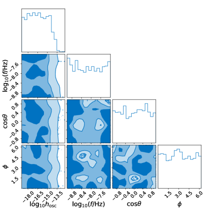
Figure 1: The posterior distributions for the parameters of the vector dark matter signal, containing the oscillation amplitude $h_{\rm{osc}}$, oscillation frequency $\log_{10}(f/\mathrm{Hz})\in[-9.0,-7.2]$, and the angles of propagation direction $\theta$ and $\phi$. These posteriors have been marginalized over oscillation phase parameters $\alpha_{e}$ and $\alpha_{p}$.

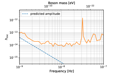
Figure 2: Upper limits on the signal amplitude $h_{\rm{osc}}$ (orange line), generated by the vector dark matter in the Galatic as a function of frequency (mass). The blue dashed line shows the model amplitude $h_{\rm{osc}}$, assuming $\rho_{\rm{\tiny{VF}}}=0.4\,\mathrm{\rm{GeV/cm^{3}}}$, given by Eq. (8). The peak in the orange curve is due to the loss in sensitivity at the frequency $1\rm{yr}^{-1}$ caused by fitting for the pulsar’s sky location and proper motion (Zhu et al., 2014).

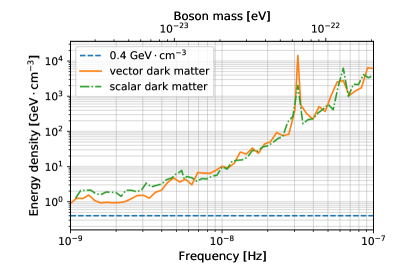
Figure 3: Upper limits on the vector dark matter density $\rho$ in the vicinity of the Earth (orange line). The green dot-dashed line denotes the upper limits on the scalar dark matter density from PPTA 12-year data set Porayko et al. (2018) and the blue dashed line denotes the measured dark matter density of $\rho_{0}=0.4\,\mathrm{\rm{GeV/cm^{3}}}$.

Fig. 1 shows the posterior distributions of the vector dark matter signal parameters after marginalizing over oscillation phases $\alpha_{e}$ and $\alpha_{p}$. Since we find no evidence of a vector dark matter signal, these posterior distributions resemble those of priors except that we are able to exclude large oscillation amplitudes, i.e., $h_{\rm{osc}}\lesssim 10^{-13.5}$. In Fig. 2, we show the $95\%$ upper limits on the oscillation amplitude $h_{\rm osc}$ as a function of frequency. We also plot the predicted amplitude according to Eq. (8) by taking the vector field dark matter density $\rho_{\rm{\tiny{VF}}}$ equal to the measured local dark matter density $\rho_{0}=0.4\,\mathrm{\rm{GeV/cm^{3}}}$, assuming that all the dark matter is composed of ultralight vector fields. The predicted amplitude is always below the upper limits, implying we cannot exclude the possibility that the vector fields with masses considered in this work constitute all the dark matter. A more intuitive picture can be obtained by translating the amplitude into the vector field dark matter energy density $\rho_{\rm{\tiny{VF}}}$ through Eq. (8) and placing the $95\%$ upper limit on the energy density, as shown in Fig. 3. As a comparison, we also plot the upper limits derived from a scalar dark matter search presented in Ref. Porayko et al. (2018). We note that the lighter mass provides tighter constraints in our search range. The strongest bound on the dark matter energy density is $1\,\mathrm{\rm{GeV/cm^{3}}}$ at the lowest frequency $10^{-9}$ Hz. This is above the local energy density of $\rho_{0}=0.4\,\mathrm{\rm{GeV/cm^{3}}}$, so we cannot place effective constraints on the mass of vector dark matter from current PTA data sets.

The results from this work are consistent with the scalar dark matter search performed with an earlier version of the PPTA data published in 2018. Specifically, our constraints on vector dark matter density $\rho_{\rm{\tiny{VF}}}<5\,\mathrm{\rm{GeV/cm^{3}}}$ for $m\lesssim 10^{-23}\,\mathrm{\rm{eV}}$ is only slightly more stringent than the scalar dark matter density limit of $6\,\mathrm{\rm{GeVcm^{-3}}}$ given by (Porayko et al., 2018). This is unsurprising because only when the vector field oscillates along a particular direction that is parallel to the line of sight to the pulsar, can we expect the timing residuals induced by the gravitational effect to be three times that caused by the scalar dark matter. However, we do not find a preferred oscillation direction of vector dark matter (see Fig. 1) in the data set.

Several cosmological and astrophysical probes can place constraints on the mass of ultralight dark matter when considering the model has only gravitational coupling. Planck cosmic microwave background data implies a bound on the ultralight dark matter energy density fraction for the $10^{-33}-10^{-24}\,\mathrm{\rm{eV}}$ mass range Hlozek et al. (2018). The Lyman-$\alpha$ forest used to trace the underlying dark matter distribution at high redshifts excludes the possibility that the ultralight particles with mass lighter than $2\times 10^{-20}\,\mathrm{\rm{eV}}$ make up all the dark matter (Rogers and Peiris, 2021). While the above constraints come from axions and their applicability to ultralight vector dark matter needs to be discussed, the black hole superradiance estimates from supermassive black hole spin measurements constrain the vector dark matter within the mass range $6\times 10^{-20}$–$2\times 10^{-17}\,\mathrm{\rm{eV}}$ (Baryakhtar et al., 2017). Although there is no consensus on the constraints on the mass of ultralight dark matter because most of the experiments are subject to their own uncertainties, it is important to note that PTA experiments can constrain the energy density of ultralight dark matter independently and determine whether dark matter is dominated by the ultralight vector particles and thus provide complementary tools to other experiments.

Looking into the future, PTAs based on the Five-hundred-meter Aperture Spherical Telescope (Nan et al., 2011), MeerKAT Bailes et al. (2020), and Square Kilometer Array (SKA) (Lazio, 2013) with wider frequency bands and large collecting areas, will increase the sensitivity significantly. In the SKA era, a conservative estimate is that 10 years of observations for the 10 best pulsars with an observing cadence of once every 14 days have the potential to constrain the contribution of ultralight dark matter down to $10\%$ of the local dark matter density for $m<10^{-23}\,\mathrm{\rm{eV}}$ (Porayko et al., 2018). In the shorter terms sensitivity improvments could be achieved through searches with the IPTA. Combining efforts from PTAs and other experiments will greatly advance our understanding of the nature of dark matter by studying a wide range of dark matter models.