Growth reduction of similarity transformed electronic Hamiltonians in qubit space

Abstract

Accurately solving the electronic structure problem through the variational quantum eigensolver (VQE) is hindered by the available quantum resources of current and near-term devices. One approach to relieving the circuit depth requirements for VQE is to “pre-process” the electronic Hamiltonian by a similarity transformation incorporating some degree of electronic correlation, with the remaining correlation left to be addressed by the circuit ansatz. This often comes at the price of a substantial increase in the number of terms to measure in the similarity transformed Hamiltonian. In this work, we propose an efficient approach to sampling elements from the complete Pauli group for $N$ qubits which minimize the onset of new terms in the transformed Hamiltonian, while facilitating substantial energy lowering. We benchmark the growth-mitigating generator selection technique for ground state energy estimations applied to models of the H₄, N₂ and H₂O molecular systems. It is found that utilizing a selection procedure which obtains the growth-minimizing generator from the set of operators with maximal energy gradient is the most competitive approach to reducing the onset of Hamiltonian terms while achieving systematic energy lowering of the reference state.

I Introduction

A broadly investigated application of the variational quantum eigensolver (VQE) is accurately solving instances of the electronic structure problem. [1, 2, 3] While the state-of-the-art in digital quantum computing hardware is rapidly improving, [4] the application of widely investigated fixed circuit ansätze, such as the unitary coupled cluster with singles and doubles (UCCSD), [5, 6, 7, 8, 9, 10, 11] can require circuit depths beyond the capability of current and near-term devices. To explore the possibilities of near-term quantum advantage, adaptive schemes within the VQE framework featuring system-specific iterative ansatz construction have been proposed. [12, 13, 14, 15, 16, 17, 18] These approaches aim to adaptively parameterize the target electronic wavefunction to desirable accuracy with a quantum circuit as shallow as possible. Such approaches feature selection of a unitary generator from a predefined operator set (“pool”). At each iteration, the operator pool elements are ranked by an importance measure. The importance measure has typically been taken to be the absolute value of the energy’s first partial derivative with respect to the generator’s free parameter. The element corresponding to the maximum value of this importance measure is then taken as generator of the current step unitary included in the quantum circuit ansatz.

While adaptive schemes have demonstrated robust numerical convergences to ground and excited electronic states to high accuracy, [12, 15, 16, 19] certain instances of the electronic structure problem may demand many iterations within an adaptive VQE scheme, leading to regrettably deep quantum circuits. One approach to reduce the depths of the required circuits is via preprocessing of the electronic Hamiltonian by an exact or approximate similarity transformation of the electronic Hamiltonian. Such transformations aim to admit a more compact circuit description of the target electronic state. In the case of exact transformation, an effective Hamiltonian is obtained as

$$\hat{H}_{\rm{eff}}=\hat{T}^{-1}\hat{H}\hat{T}.$$ (1)

Approximations to $\hat{H}_{\rm{eff}}$ can be obtained by neglecting higher order terms in the Baker-Campbell-Hausdorff (BCH) expansion of $\hat{T}^{-1}\hat{H}\hat{T}$, for instance. It is desirable to utilize $\hat{T}$ which admits a tractable exact transformation of $\hat{H}$, as in this case $\hat{H}_{\rm{eff}}$ and $\hat{H}$ are formally isospectral. For Hamiltonian preprocessing prior to a variational treatment, it is also desirable that the transformation is unitary, preserving the Hermitian property of the Hamiltonian. Hence, exact unitary transformation of $\hat{H}$ ensures that a variational solution to $\hat{H}_{\rm{eff}}$ is lower bounded by the ground state energy of $\hat{H}$. Nevertheless, often motivated by computational feasibility, many recent contributions have considered preprocessing the electronic Hamiltonian with approximate transformations. [20, 21, 22, 19, 23]

An adaptive method employing exact and unitary Hamiltonian transformations formulated in the qubit space algebra is the iterative qubit coupled cluster (iQCC) approach.[15] The iQCC method features selection of individual Pauli products, i.e., tensor products of the Pauli matrices and the single qubit identity,

$$\hat{P}_{\alpha}=\hat{\sigma}_{1}^{(\alpha)}\otimes\hat{\sigma}_{2}^{(\alpha)}\ldots\otimes\hat{\sigma}_{N}^{(\alpha)},\quad\hat{\sigma}_{i}^{(\alpha)}\in\{\hat{x},\hat{y},\hat{z},\hat{1}\},$$ (2)

as unitary generators. A feature which distinguishes the iQCC method from other adaptive approaches is the usage of an unrestricted operator pool. The iQCC operator pool is taken to be the set of all $4^{N}-1$ possible $N$ qubit Pauli products, where structure in the qubit-mapped electronic Hamiltonian $\hat{H}$ and reference state facilitate an operator ranking procedure which scales polynomially in $N$. [15] Following optimization of the generators’ associated variational amplitudes, the unitary is used to transform the current step Hamiltonian in the qubit space. The iQCC method has demonstrated systematic convergence towards ground state and excited state energies for problems requiring up to $72$ logical qubits. [15, 24] Furthermore, a posteriori corrections have been developed to further increase accuracy of iQCC energy estimates. [25] The employed Hamiltonian transformations are exact, where formally all BCH terms are summed in acquiring $\hat{H}_{\rm{eff}}$ with no neglecting of high body fermionic terms. Hence, while iQCC is a formally variational unitary downfolding procedure, the effective iQCC Hamiltonians have demonstrated rapid increase in the number of terms, particularly accentuated for the initial iterations. It has been elucidated that the rate of Pauli product increase diminishes at later iterations. [24] Nevertheless, the main computational expense of the iQCC procedure arises from the introduction of a prohibitive number of Pauli products in the iQCC effective Hamiltonians.

In this work, we consider screening the Pauli product operator pool for elements which not only guarantee energy lowering via their energy gradient importance measure, but elements which minimize onset of new Pauli products in the exactly transformed current step effective Hamiltonian. This is accomplished by introducing a novel operator pool sampling scheme for the iQCC methodology which is sensitive to the introduction of new Pauli products in the transformed Hamiltonian. Further, we introduce an efficient approach to identifying elements from the exponentially sized unrestricted operator pool which minimize the growth of the transformed Hamiltonian while possessing a fixed energetic gradient magnitude. To balance consideration of energetic gradients and the expected increase of terms when selecting from the operator pool, we introduce a parameterized scoring function assigned to pool elements which acts as a cumulative importance measure.

The rest of the paper is structured as follows. In Section II, we review the necessary aspects of the iQCC methodology, and introduce an operator pool importance measure which takes into account the expected growth of candidates for selection. In Section III, we perform numerical tests for the H₄, N₂, and H₂O systems in strongly correlated regimes. We provide a discussion and an outlook on future perspectives in Section IV.

II Theory

II.1 Iterative Qubit Coupled Cluster

The iterative qubit coupled cluster (iQCC) method is an adaptive variational quantum algorithm utilizing effective Hamiltonians which has demonstrated systematic convergence towards ground state energies. [15, 24] The iQCC method involves iteratively unitarily transforming the qubit-space Hamiltonian $\hat{H}$ with parameterized unitary transformations. [15] An iteration begins with selection of $N_{\rm{gen}}$ Pauli products $\{\hat{P}_{\alpha}\}_{\alpha=1}^{N_{\rm{gen}}}$, which define variational ansatz

$$\hat{U}_{\rm{QCC}}=\prod_{k=1}^{N_{\rm{gen}}}e^{-i\tau_{\alpha}\hat{P}_{\alpha}/2}.$$ (3)

The energy is then optimized with respect to amplitudes $\bm{\tau}=\{\tau_{\alpha}\}_{\alpha=1}^{N_{\rm{gen}}}$ as

$$E_{K}=\min_{\bm{\tau}}\bra{0}\hat{U}_{\rm{QCC}}^{\dagger}(\bm{\tau})\hat{H}^{(K)}\hat{U}_{\rm{QCC}}(\bm{\tau})\ket{0},$$ (4)

where $\ket{0}$ is a reference computational basis state (a Slater determinant in the fermion-to-qubit mapped orbital basis), and $K=0,1\ldots$ denotes the iteration number. Pauli products are included in $\hat{U}_{\rm{QCC}}$ based on the magnitude of the first derivative of the energy with respect to their associated variational amplitude,

$$g_{\alpha} =\left|\frac{\partial E_{K}}{\partial\tau_{\alpha}}\Big{|}_{\tau_{\alpha}=0}\right|,$$ (5)

where

$$\frac{\partial E_{K}}{\partial\tau_{\alpha}}\Big{|}_{\tau_{\alpha}=0} =\frac{\partial}{\partial\tau_{\alpha}}\bra{0}e^{i\tau_{\alpha}\hat{P}_{\alpha}/2}\hat{H}^{(K)}e^{-i\tau_{\alpha}\hat{P}_{\alpha}/2}\ket{0}$$ (6)

$$=-\frac{i}{2}\bra{0}[\hat{H}^{(K)},\hat{P}_{\alpha}]\ket{0}.$$ (7)

Pauli products with the highest values of $g_{\alpha}$ are selected for inclusion in $\hat{U}_{\rm{QCC}}$. Further, the exponentials in Eq.(3) are ordered by ascending gradient magnitude (the highest gradient term acts directly on the reference wavefunction). Unlike other adaptive VQE schemes featuring a predefined and restricted operator pool (such as generators arising from fermionic single and double excitations with respect to $\ket{0}$), the iQCC method utilizes the unrestricted pool of all non-trivial $N$-qubit Pauli products, $\{\hat{P}_{\alpha}\}_{\alpha=1}^{4^{N}-1}$. Thus, to achieve an efficient screening of the operator pool, one can not directly evaluate $g_{\alpha}$ for all pool elements individually, as is typically done in other adaptive VQE schemes. Instead, utilizing structure in the qubit-mapped $\hat{H}$ and reference state $\ket{0}$, one can constructively obtain the elements in this unrestricted Pauli product pool with non-zero gradient $g_{\alpha}$ using a classical algorithm efficient in the number of qubits $N$ and number of Pauli products in the qubit-mapped Hamiltonian, $M$. We review the derivation of this procedure in Appendix A. To summarize the main result, the qubit-space Hamiltonian may be expressed as

$$\hat{H}=\sum_{i}\left(\sum_{j}c_{j}^{(i)}\hat{Z}_{j}^{(i)}\right)\hat{X}_{i},$$ (8)

where $\hat{Z}_{j}^{(i)}$ ($\hat{X}_{i}$) are tensor products of Pauli $\hat{z}$ ($\hat{x}$) operators. We partition $\{\hat{P}_{\alpha}\}_{\alpha=1}^{4^{N}-1}$ under the equivalence relation: if Pauli products $\hat{P}_{\alpha}$ and $\hat{P}_{\beta}$ can be expressed (up to a phase) as $\hat{Z}_{\alpha}\hat{X}_{\alpha}$ and $\hat{Z}_{\beta}\hat{X}_{\alpha}$ respectively, and that $\hat{P}_{\alpha}$ and $\hat{P}_{\beta}$ possess the same number of Pauli $\hat{y}$ operators modulo $2$, then $\hat{P}_{\alpha}\sim\hat{P}_{\beta}$. If $\hat{P}_{\alpha}\sim\hat{P}_{\beta}$, then $g_{\alpha}=g_{\beta}$. The gradient magnitude of Pauli product $\hat{P}_{\alpha}=\hat{Z}_{\alpha}\hat{X}_{\alpha}$ (ignoring phase) is zero unless two criteria are met: 1) the Pauli product possesses an odd number of Pauli $\hat{y}$ operations (the size of overlap of supports of $\hat{Z}_{\alpha}$ and $\hat{X}_{\alpha}$ is odd), and 2) $\hat{X}_{\alpha}=\hat{X}_{i}$ for some $\hat{X}_{i}$ in Eq. (8). This lets us constructively characterize the non-zero gradient partitions of the Pauli product pool by classically computing the gradient magnitude for each $\hat{X}_{i}$ in Eq. (8). Elements from the highest gradient partitions are selected for inclusion in $\hat{U}_{\rm{QCC}}$. We denote the set of unique non-zero gradient magnitudes as $\{g^{(k)}\}_{k}$, where all $\hat{P}_{\alpha}$ in partition $k$ have $g_{\alpha}=g^{(k)}$.

Following optimization of the $\hat{U}_{\rm{QCC}}$ amplitudes, the next-step Hamiltonian is obtained as $\hat{H}^{(K+1)}=\hat{U}_{\rm{QCC}}^{\dagger}(\bm{\tau}^{\prime})\hat{H}^{(K)}\hat{U}_{\rm{QCC}}(\bm{\tau}^{\prime})$ using the optimal amplitudes, $\bm{\tau}^{\prime}=\operatorname*{arg\,min}_{\bm{\tau}}E_{K}$. This transformation is classically performed via recursion, where transformation generated by a single Pauli product gives

$$e^{i\tau^{\prime}_{\alpha}\hat{P}_{\alpha}/2}\hat{H}e^{-i\tau^{\prime}_{\alpha}\hat{P}_{\alpha}/2}= \hat{H}-\frac{i}{2}\sin{\tau^{\prime}_{\alpha}}[\hat{H},\hat{P}_{\alpha}]$$

$$+\frac{1}{2}\left(1-\cos\tau^{\prime}_{\alpha}\right)\left(\hat{P}_{\alpha}\hat{H}\hat{P}_{\alpha}-\hat{H}\right).$$ (9)

The next iQCC iteration begins with partition screening of the Pauli product pool with respect to $\hat{H}^{(K+1)}$, and the procedure is repeated until a convergence criterion is met, such as in $E_{K}$’s or via norm of $\{g^{(k)}\}$.

II.2 Assessing Hamiltonian growth

For adaptive VQE schemes employing effective Hamiltonians, the number of Pauli products in the transformed Hamiltonian is a crucial performance metric, as classical and quantum measurement resource requirements will generally increase with $M$. However, the exact number of measurements required to estimate the energy to a desired precision will be dependent on the energy estimator being employed, as well as the current step trial wavefunction. Let $\mathcal{H}^{(K)}=\{\hat{P}_{i}\}_{i=1}^{M}$ denote the set of Pauli products in $\hat{H}^{(K)}$. By inspection of Eq. (II.1), new terms in the Hamiltonian transformed with $\exp(-i\tau_{\alpha}^{{}^{\prime}}\hat{P}_{\alpha}/2)$ are introduced only by $[\hat{H},\hat{P}_{\alpha}]$. Since two Pauli products either commute or anticommute, $\hat{P}_{\alpha}\hat{H}\hat{P}_{\alpha}$ will not introduce Pauli products not already in $\hat{H}$, since $\hat{P}_{\alpha}\sum_{i}c_{i}\hat{P}_{i}\hat{P}_{\alpha}=\sum_{i}c_{i}\theta_{i}\hat{P}_{i}$, where $\theta_{i}$ equals $1$ ($-1$) if $\hat{P}_{i}$ and $\hat{P}_{\alpha}$ commute (anticommute). Further, any commutator $[\hat{P}_{i},\hat{P}_{\alpha}]$ in $[\hat{H},\hat{P}_{\alpha}]=\sum c_{i}[\hat{P}_{i},\hat{P}_{\alpha}]$ will contribute a new term not found in $\mathcal{H}^{(K)}$ if $\hat{P}_{i}$ and $\hat{P}_{\alpha}$ anticommute and $[\hat{P}_{i},\hat{P}_{\alpha}]=2\hat{P}_{i}\hat{P}_{\alpha}$ is not proportional to a term in $\mathcal{H}^{(K)}$. Therefore, we can quantify the growth incurred by transforming the Hamiltonian with $\exp(-i\tau_{\alpha}^{{}^{\prime}}\hat{P}_{\alpha}/2)$ as the number of terms in $[\hat{H}^{(K)},\hat{P}_{\alpha}]$ that are not found in $\mathcal{H}^{(K)}$. We denote this quantity as $\gamma_{\alpha}$, which serves as an analytically exact upper bound to the increase in number of terms upon conjugating the current step Hamiltonian with $\exp(-i\tau_{\alpha}^{{}^{\prime}}\hat{P}_{\alpha}/2)$,

$$|\mathcal{H}^{(K+1)}|\leq|\mathcal{H}^{(K)}|+\gamma_{\alpha}.$$ (10)

The case of inequality arises when there are term cancellations, or when magnitude of a Pauli product coefficient in the resulting Hamiltonian falls below a precision threshold, and is hence omitted. Such cases will be dependent on the value of $\tau_{\alpha}^{{}^{\prime}}$, which are not accounted for in the analytical growth consideration.

In the context of an adaptive Hamiltonian transformation, we generally wish to select Pauli products from the pool with high $g_{\alpha}$ and low $\gamma_{\alpha}$. Similarly to how energetic gradients can not be directly assessed for the exponential number of elements in the Pauli group, assessing growth explicitly for all pool elements is computationally expensive. Instead, we devise efficient classical algorithms for obtaining the pool element with smallest $\gamma_{\alpha}$ within a given gradient partition. These algorithms and their derivation are included in Appendix B. For a given partition $k$, we denote the minimal growth by $\gamma^{(k)}$, i.e., the lowest growth observed in the set of Pauli products with gradient $g^{(k)}$. We can hence use both $g^{(k)}$ and $\gamma^{(k)}$ in determining which partition of the Pauli product pool will be sampled from. In the next section, we introduce a parameterized scoring function which ranks the partitions of the Pauli product pool based on both $g^{(k)}$’s and $\gamma^{(k)}$’s.

II.3 Hybrid operator importance measures

The majority of adaptive ansatz schemes, including iQCC, have used proxies for expected energy lowering such as energetic gradients $g_{\alpha}$’s as the sole importance measure when considering which elements from the operator pool should be included in the ansatz at a given iteration. In the context of an effective Hamiltonian theory, we can introduce another importance measure based on the worst-case increase in the number of Hamiltonian Pauli products upon transformation generated by a given element. To consider both energetic gradients and growth in selecting from the operator pool, we introduce score function $s^{(k)}$ assigned to partitions of the pool. Since energetic convergence will largely be determined by the energetic gradients of the chosen generators, we only consider scoring the $P$ highest gradient pool partitions. We define this cumulative score function as

$$s^{(k)}=a\tilde{g}^{(k)}-\left(1-a\right)\tilde{\gamma}^{(k)},$$ (11)

where $\tilde{g}_{k}$ and $\tilde{\gamma}^{(k)}$ are normalized energetic gradients and growth, respectively,

$$\tilde{g}^{(k)} =g^{(k)}\left(\frac{\sum_{i=1}^{P}g^{(i)}}{P}\right)^{-1},$$ (12)

$$\tilde{\gamma}^{(k)} =\gamma^{(k)}\left(\frac{\sum_{i=1}^{P}\gamma^{(i)}}{P}\right)^{-1}.$$ (13)

Real parameter $a\in[0,1]$ in Eq. (11) acts as a bias for energetic gradient. For instance, sampling from the highest energy gradient partition regardless of minimum growth estimates is accomplished by setting $a=1$.

III Numerical assessments

Within this section we benchmark utilization of iQCC effective Hamiltonians obtained with operator selection employing the hybrid importance measure Eq. (11) for polyatomic systems exhibiting strong correlation effects. We compare to the canonical sampling choice used in the conventional iQCC methodology. [15] To recall, a gradient partition of the Pauli group is the set of $2^{N-1}$ Pauli products possessing an odd number of $\hat{y}$ operations with identical $\hat{X}_{\alpha}$ in factorization $\hat{P}_{\alpha}=\hat{Z}_{\alpha}\hat{X}_{\alpha}$ omitting multiplicative phase. The canonical sample from partition characterized by $\hat{X}_{\alpha}$ is defined by placing a single $\hat{y}$ operation on the index of the first non-trivial qubit acted on by $\hat{X}_{\alpha}$, the remaining non-trivial qubit indices are populated with $\hat{x}$ operators. For example, $\hat{y}_{1}\hat{x}_{2}\hat{x}_{3}\hat{x}_{4}$ is the canonical iQCC operator choice from a partition characterized by $\hat{X}_{\alpha}=\hat{x}_{1}\hat{x}_{2}\hat{x}_{3}\hat{x}_{4}$. Below, we outline the procedure for growth mitigated iQCC, denoted GM($a$)-iQCC, where $a$ denotes the gradient bias utilized in scoring function $s(a)$ (see Eq. (11)). We use $s(a)$ with several different gradient bias values for assessment. All iQCC calculations herein use $N_{\rm{gen}}=1$, hence the highest gradient partition is always selected from in the canonical scheme. Explicitly, the employed procedure for obtaining the $K^{\rm{th}}$ step effective Hamiltonian in the GM($a$)-iQCC scheme is:

1. Obtain description of the Pauli group partitioning for $\hat{H}^{(K-1)}$ (see Appendix A). Let $\{g^{(k)}\}_{k=1}^{P}$ be the set of the $P$ highest energetic gradient magnitudes Eq. (5).

2. For each of the $P$ highest gradient partitions, obtain the lowest growth incurring element (see Appendix B). In doing so, we obtain the minimal growth value of the top $P$ partitions $\{\gamma^{(k)}\}_{k=1}^{P}$.

3. Compute the scores $\{s^{(k)}\}_{k=1}^{P}$ of the top $P$ partitions using chosen bias $a$, and computed $\{g^{(k)}\}_{k=1}^{P}$ and $\{\gamma^{(k)}\}_{k=1}^{P}$ (see Eq. (11)).

4. Select $\hat{P}_{K}$ corresponding to the growth minimizing element of the top scoring partition according to $\{s^{(k)}\}_{k=1}^{P}$.

5. Perform optimization

   $$\min_{\tau_{K}}E_{K}(\tau_{K})=\bra{0}e^{i\tau_{K}\hat{P}_{K}/2}\hat{H}^{(K-1)}e^{-i\tau_{K}\hat{P}_{K}/2}\ket{0}.$$ (14)

   Converged $\min_{\tau_{K}}E_{K}(\tau_{K})$ is taken as the $K^{\rm{th}}$ step of the energy estimation.

6. Using $\tau_{K}^{{}^{\prime}}=\operatorname*{arg\,min}E_{K}(\tau_{K})$, obtain $K^{\rm{th}}$ step effective Hamiltonian $\hat{H}^{(K)}$ after transformation Eq. (II.1).

It should be emphasized that Step 4 features the selection of the growth minimizing element of the highest scoring partition. For instance, the $s(1)$ parameterization results in the growth minimizing element of the highest energy gradient partition being selected for at each step in the GM($1$)-iQCC procedure. This differentiates GM($1$)-iQCC from iQCC utilizing the canonical sampling scheme, while also always selects from the highest gradient partition, however with no effort made to minimize growth by the specific Pauli product chosen within the partition.

For all systems studied herein, the Jordan-Wigner encoding was utilized in obtaining fermion-to-qubit mapped Hamiltonians through the OpenFermion package,[26] with no qubit tapering procedures employed. Hence a fermionic Hamiltonian defined over $N_{\rm{mo}}$ active molecular orbitals (MOs) results in a qubit-space Hamiltonian of $N=2N_{\rm{mo}}$ qubits. All fermionic Hamiltonians were resolved in the restricted Hartree-Fock (RHF) MO basis. All iQCC calculations utilize a fixed reference state taken to be the qubit-space RHF state, which corresponds to a computational basis state under the mapping of RHF spin orbitals to qubits.

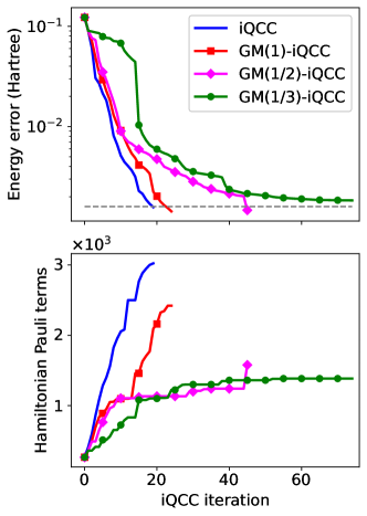
Figure 1: Comparison of iQCC procedure convergences applied to the H₄ chain in the STO-3G basis set with an equidistant H$-$H separation of $1.5$ Å. The energy error is the difference between the iQCC energy estimate at a given iteration and the FCI energy. The horizontal grey dashed line indicates an error of $1$ kcal/mol ($1.6$ milli-Hartree).

III.1 H₄ chain

The electronic Hamiltonian for the linear H₄ chain was generated in the minimal STO-3G basis set with an equidistant H$-$H separation of $R=1.5$ Å. No freezing of orbitals was performed, resulting in a Hamiltonian defined over $4$ MOs and hence a $N=8$ qubit mapped Hamiltonian. Energy errors are taken with respect to the full configuration interaction (FCI) solution, obtained via exact diagonalization. In the GM($a$)-iQCC procedures, we use $r=\lceil\log_{2}M\rceil$ in the growth minimizing search (see Algorithm 1 of Appendix B).

In Figure 1, convergence of iQCC energies utilizing various parameterizations of the partition score function are compared with the canonical sampling scheme. It is observed that operator selection via the $s(1)$ parameterization, utilized in GM($1$)-iQCC, gives a similar convergence trajectory to canonical iQCC selection, only requiring a few more iterations to achieve a desired accuracy of $1$ kcal/mol ($1.6$ milli-Hartree). This is expected, since in both schemes, the highest energy gradient partition is selected from for the current step Hamiltonian. However, while the schemes sample from the same partition for the initial Hamiltonian, this generally changes for later effective Hamiltonians which have different gradient values for the pool partitions. Hence we still expect slight deviations in their energy convergence trajectories. While selection using $s(1)$ demonstrates energetic convergence on par with that obtained using canonical selection, only a decrease of $\sim 20\%$ in the number of Pauli products in the effective Hamiltonians required for achieving an accuracy of $1$ kcal/mol is observed. However, comparing the procedures with fixed iteration number, there are several instances where sampling via $s(1)$ provides substantially reduced Pauli product counts for effective Hamiltonians, e.g., $K=10$, where the GM($1$)-iQCC effective Hamiltonian provides a $\sim 50\%$ reduction in the number of Pauli products in the effective Hamiltonian compared to the canonical selection scheme.

More significant reductions in effective Hamiltonian Pauli product counts are obtained using partition score function with non-zero weight placed on growth value. For instance, $s(1/2)$ provides an effective Hamiltonian with $\sim 48\%$ less terms than canonical sampling to achieve an error of less than $1$ kcal/mol. However, since in general, the GM($1/2$)-iQCC procedure no longer samples from the highest gradient partition at each step, we observe that the rate of energetic convergence is decreased substantially. While offering the most reduced effective Hamiltonians at earlier iterations, the $s(1/3)$ selection fails to systematically converge the iQCC energy beyond an error of $1.84$ milli-Hartree. Further, the GM($1/3$)-iQCC energies are significantly higher than the energies obtained via the other selection schemes for the earlier iterations. We attribute the poor convergence of the $s(1/3)$ selection scheme to be a symptom of over-biasing the growth consideration. In this regime, generators are being selected more so by their expected onset of new Pauli products in the next-step effective Hamiltonian, rather than their energy gradients. Since energetic convergence will largely be dictated by the gradients of the selected generators, it is crucial to not under-weight the importance of energetic gradients $g^{(k)}$ in Eq. (11).

III.2 N₂ molecule

We perform assessment of GM-iQCC applied to N₂ in an active space derived from the cc-pVDZ basis set. The active space is constituted by six electrons in six molecular orbitals ($6$e,$6$o), the minimal complete active space to describe the triple bond formation, resulting in a $N=12$ qubit-mapped Hamiltonian. The three highest energy occupied MOs and three lowest energy unoccupied MOs in the converged RHF solution form the active space. Energy errors are reported relative to the complete active space configuration interaction (CASCI) solution, obtained via exact diagonalization of the active space Hamiltonian. The GM($a$)-iQCC procedures utilize $r=\lceil\log_{2}M\rceil$ in the growth minimizing search.

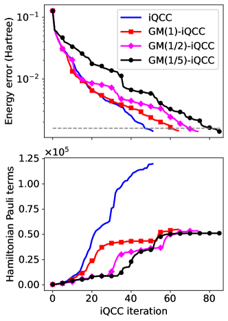
Figure 2: Comparison of iQCC procedure convergences applied to a CAS($6$e, $6$o) N₂ model in the cc-pVDZ basis set with a bond distance of $1.5$ Å. The energy error is the difference between the iQCC energy estimate at a given iteration and the CASCI energy. The horizontal grey dashed line indicates an error of $1$ kcal/mol ($1.6$ milli-Hartree).

In Figure 2 we benchmark energetic convergences of iQCC procedures employing parameterized partition score function for selection along with the canonical selection at the stretched bond distance $R=1.5$ Å. The canonical, $s(1)$, and $s(1/2)$ selection schemes give similar energetic convergence for the first $\sim 15$ iterations. As expected, iQCC and GM($1$)-iQCC share similar convergence trajectories, requiring $52$ and $65$ iterations to achieve an error within $1$ kcal/mol, respectively. Significantly, the effective $K=65$ GM($1$)-iQCC effective Hamiltonian consists of $5.5\times 10^{4}$ terms, a $\sim 46\%$ reduction compared to the $K=52$ effective iQCC Hamiltonian of $1.2\times 10^{5}$ terms obtained via canonical selection.

The $s(1/2)$ selection procedure provides drastically reduced term counts for effective Hamiltonians up to the $30^{\rm{th}}$ iteration, at which point a rapid onset of terms in the subsequent iterations brings the Pauli product counts to be comparable with the $s(1)$ procedure at similar iterations. By this iteration, all schemes’ effective Hamiltonians provide substantially improved reference energies, however the GM($1$)-iQCC and GM($1/2$)-iQCC procedures offering substantially reduced effective Hamiltonian Pauli product counts. For instance, at $K=20$, the canonical selection provides an effective Hamiltonian of $3.6\times 10^{4}$ Pauli products and an energy error of $6.9$ milli-Hartree, while the $s(1/2)$ selection gives an effective Hamiltonian of $7.6\times 10^{3}$, demonstrating a $\sim 79\%$ reduction, with a comparable energy error of $8.7$ milli-Hartree.

While adaptive ansatz schemes inherently yield non-differentiable energy surfaces, it is desirable that the growth-mitigated iQCC relative errors over the considered bond lengths are not systematically worse than those of the standard iQCC procedure. To this end, potential energy surfaces PESs for the N₂ model obtained via iQCC and GM($1$)-iQCC procedures are shown in Figure 3. To assess the quality of PESs obtained via GM($1$) and standard iQCC procedures at various levels of convergence, we utilize a convergence criterion based on the gradient norm, i.e., the procedure exits when $\sum_{k}|g^{(k)}|\leq\epsilon_{i}$ for predefined threshold $\epsilon_{i}$. Figure 3 includes comparison of the GM($1$) and standard iQCC procedures at three gradient convergence thresholds: $\epsilon_{1}=0.1$, $\epsilon_{2}=0.2$, and $\epsilon_{3}=0.3$ Hartree.

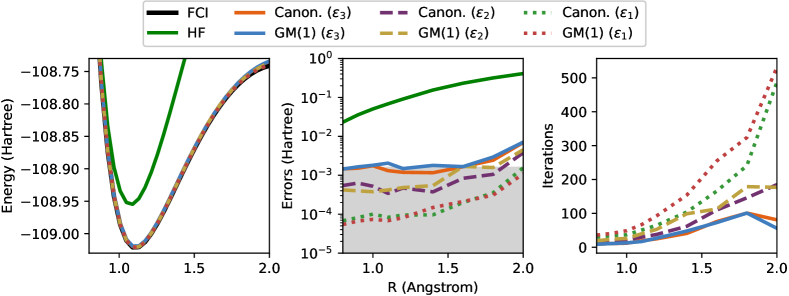
Figure 3: Potential energy surfaces obtained by the standard iQCC (“Canon.”) and GM($1$)-iQCC procedures applied to the CAS($6$e, $6$o) N₂ model in the cc-pVDZ basis set. The energy error is the difference between the iQCC energy estimate at a given iteration and the CASCI energy. The grey shaded area of the middle plot indicates errors within $1$ kcal/mol ($1.6$ milli-Hartree) of the exact CASCI energy.

For fixed convergence threshold, the standard and GM($1$) iQCC procedures demonstrate similar errors and number of required iterations at the majority of bond lengths. Utilizing thresholds $\epsilon_{1}$, $\epsilon_{2}$, and $\epsilon_{3}$, the standard iQCC procedures respectively achieve non-parallelity errors (NPEs) of $1.5\times 10^{-3}$, $3.4\times 10^{-3}$, and $5.7\times 10^{-3}$, while the GM($1$) procedures obtain NPEs of $1.0\times 10^{-3}$, $4.1\times 10^{-3}$, and $5.6\times 10^{-3}$. The NPE is defined as the difference between maximum error and minimum error relative to the exact CASCI energy obtained over all considered bond lengths. With considerably similar performance in terms of energetic errors and number of iterations required for convergence, it is to be noted that the advantage of the GM($1$) procedure lies in the reduced number of Hamiltonian terms along the iQCC procedure.

In Table 1, benchmarking of simulated VQE application of iQCC and GM($a$)-iQCC pre-processed Hamiltonians is demonstrated, with comparisons to other classical electronic structure and VQE computations employing the original Hamiltonian. All classical electronic structure calculations were carried out using the Psi4 quantum chemistry package.[27] The strongly correlated nature of the N₂ model with a bond length of $1.5$ Å leads to a challenging case for the post-HF classical electronic structure methods, evident by the energetic errors of the coupled-cluster with singles and doubles (CCSD) and Møller-Plesset second order perturbation theory (MP2) energies being several milli-Hartree. Similarly, the dissociation of the linear H₄ chain to separated hydrogen atoms is a prototypical model exhibiting strong correlation effects. For the single point energy evaluation used for assessment, we set the equidistant H$-$H separation as $1.5$ Å and utilize the STO-3G minimal basis. Furthermore, benchmarking against the VQE employing the UCCSD ansatz as implemented in the Tequila package is performed. The UCCSD ansatz likewise fails to achieve accuracy within $1$ kcal/mol for these problem instances. All methods involving VQE computations utilizing iQCC or GM($a$)-iQCC preprocessed qubit space Hamiltonian feature transformation including only a single generator per iteration. For example, method “GM($1$)-iQCC($10$)” in Table 1 denotes a preprocessed Hamiltonian obtained after twenty iterations of the iQCC procedure employing the $s(1)$ scoring function for the single generator selection performed at each iteration. Subsequently, the QCC method utilizing ten generators is applied to the final effective Hamiltonian. The energy error reported is the difference between the final optimized QCC energy and the CASCI energy. In general, the iQCC preprocessed Hamiltonians allow for much shallower quantum circuits, at the expense of more Pauli products in the Hamiltonian entering the QCC procedure. The GM($a$)-iQCC procedure likewise produces quantum resource reductions competitive with iQCC, while offering substantially reduced effective Hamiltonian Pauli product counts.

Table 1: Comparison of methods applied to models in the strongly correlated regime, namely CAS($6$e, $6$o) N₂ in the cc-pVDZ basis set and a linear H₄ chain in the STO-$3$G basis set. Both the N$-$N bond distance and the equidistant H$-$H separation were set to $R=1.5$ Å, where both systems possess a high degree of orbital degeneracies. The HF, MP2, and CCSD computations were carried out using the Psi4 package. [27] The UCCSD calculation were performed using the Tequila package, where the cluster operator was obtained in closed-shell form before a first-order Trotterization. [28] QCC($N_{\text{ent}}$) denotes the QCC ansatz constructed from $N_{\text{ent}}$ selected generators. (GM($a$)-)iQCC($N_{\text{ent}}$) denotes the QCC($N_{\text{ent}}$) procedure using (GM($a$)-)iQCC preprocessed Hamiltonian. All preprocessed Hamiltonians were obtained after $K=20$ iterations. Errors are reported in milli-Hartree. The number of Pauli products in the Hamiltonian utilized in state vector VQE simulation is denoted by $M$. The reported CNOT counts were obtained via circuit compilation using the Tequila package with the Qiskit backend. [29]

Method	N2				H4
	Error	$M$	CNOTs	Circuit parameters	Error	$M$	CNOTs	Circuit parameters
HF	$192$	-	-	-	$167$	-	-	-
CCSD	$8.02$	-	-	-	$-1.47$	-	-	-
MP2	$-16.8$	-	-	-	$80.5$	-	-	-
UCCSD	$2.84$	$247$	$4512$	$30$	$2.59$	$185$	$1280$	$12$
QCC($10$)	$14.6$	$247$	$60$	$10$	$3.30$	$185$	$60$	$10$
iQCC($10$)	$4.66$	$36281$	$88$	$10$	$0.522$	$3024$	$80$	$10$
GM($1$)-iQCC($10$)	$4.62$	$21992$	$68$	$10$	$0.825$	$2096$	$84$	$10$
GM($\frac{1}{2}$)-iQCC($10$)	$7.48$	$8567$	$92$	$10$	$1.62$	$1133$	$72$	$10$
QCC($50$)	$1.69$	$247$	$300$	$50$	$0.161$	$185$	$252$	$50$
iQCC($50$)	$0.670$	$36281$	$452$	$50$	$4.36\times 10^{-2}$	$3024$	$300$	$50$
GM($1$)-iQCC($50$)	$0.814$	$21992$	$416$	$50$	$5.00\times 10^{-3}$	$2096$	$328$	$50$
GM($\frac{1}{2}$)-iQCC($50$)	$1.22$	$8567$	$436$	$50$	$4.65\times 10^{-3}$	$1133$	$316$	$50$

III.3 H₂O molecule

As a larger scale example, we compare performance of the first few iterations of iQCC and GM($1$)-iQCC for H₂O in the 6$-$31G(d) basis set. The lowest-energy MO, corresponding to the $1s$ atomic orbital of the oxygen atom, was frozen, with the remaining $18$ MOs constituting the active space, yielding a $36$ qubit Hamiltonian. A symmetric O$-$H bond distance of $1.5$ Å was used, with H$-$O$-$H angle set to $107.60^{\circ}$. The initial qubit space Hamiltonian, obtained via the Jordan-Wigner transformation of the fermionic Hamiltonian in the canonical orbital basis, contains $41915$ Pauli products. To assess the relative quality of iQCC energies obtained via the canonical and hybrid operator selection scheme, we obtain energetic errors with respect to the CASCI energy, obtained via Davidson diagonalization in the determinantal basis using the GAMESS package. [30]

We compare the canonical iQCC and GM($1$)-iQCC procedures in Table 2. In this instance, we use $r=\left\lceil M/10\right\rceil$, as the growth minimizing search using $r=\lceil\log_{2}M\rceil$ could not find the growth minimizing element in the highest gradient partition for the initial Hamiltonian. This can arise when there exists a Pauli product in the searched partition which incurs a low growth as a result from commuting with an anomalously large number of terms in the Hamiltonian. For the first six iterations, the canonical choice and the growth minimizing choice found within the highest gradient partition via the $s(1)$ procedure provide identical optimized trial energies up to $10^{-4}$ Hartree. The reduced proliferation of new Pauli products in the GM($1$)-iQCC procedure becomes pronounced as further iterations are performed. For the eighth iteration, a $43.5$ percent reduction in terms using the $s(1)$ selection procedure ($2.17\times 10^{5}$ Pauli products) compared to the canonical selection ($3.84\times 10^{5}$ Pauli products) is observed. Furthermore, the generators selected along the $s(1)$ iQCC procedure also provide a slightly lower optimized energy by the eighth iteration compared to the iQCC procedure employing the canonical selection.

Table 2: Comparison of the iQCC and GM($1$)-iQCC procedures applied to the $36$ qubit H₂O model in the 6$-$31G(d) basis with symmetric bond length of $1.5$ Å. Numerics for the iQCC and GM($1$)-iQCC methods for a given iteration are tabulated in uncoloured and grey rows respectively.

Iteration	Energy error (Hartree)	Pauli products
$1$	$0.2319$	$5.63\times 10^{4}$
	$0.2319$	$5.63\times 10^{4}$
$2$	$0.2293$	$6.79\times 10^{4}$
	$0.2293$	$6.65\times 10^{4}$
$4$	$0.2092$	$9.63\times 10^{4}$
	$0.2092$	$9.12\times 10^{4}$
$6$	$0.2048$	$1.82\times 10^{5}$
	$0.2048$	$1.41\times 10^{5}$
$8$	$0.2023$	$3.84\times 10^{5}$
	$0.2016$	$2.17\times 10^{5}$

IV Discussion

In this work, we have introduced an operator pool importance measure which takes into account the expected onset of terms in the iteratively transformed Hamiltonian. The hybrid importance measure, which has contributions from expected growth and energetic gradients, was utilized in the selection of iQCC generators for molecular systems in strongly correlated regimes. Due to the exponential size of the operator pool employed, i.e., the $N$-qubit Pauli group, efficient algorithms to finding growth-minimizing elements were devised which avoid exhaustively computing the growth for all possible elements. The benefit of utilizing the full Pauli group as the operator pool is the potential for selecting Pauli products which occur in arbitrary rank fermionic excitations. Furthermore, it circumvents the problem of “barren plateaus” in energy optimization,[31] since the selected generators are always of non-zero gradient by construction, and this selection is exhaustive over a complete operator basis. It was found that so long as biasing towards energetic gradients is not made too small in the pool partition score function, we retain robust energetic convergence towards FCI and CASCI energies, while achieving significant reductions in the number of resulting Hamiltonian Pauli products. Energetic convergences when using score function $s(1)$ were on par with the canonical iQCC selection procedure, while the former achieved up to a $\sim 50\%$ reduction in the number of resulting Hamiltonian Pauli products to achieve an energy error within $1$ kcal/mol. Placing greater bias towards minimizing growth can substantially reduce the size of early iteration effective Hamiltonians, however such a bias can impede energy lowering at later iterations. We hence consider the GM($1$)-iQCC procedure to be the most competitive approach to mitigating Hamiltonian growth while substantially reducing quantum resource requirements. Similar to the canonical iQCC procedure, the Hermitian character and eigenspectrum are formally conserved in the effective Hamiltonians, differentiating this approach from the large majority of efforts in VQE Hamiltonian preprocessing. However, the GM($1$)-iQCC procedure offers substantially smaller effective Hamiltonians compared to iQCC, while yielding competitive energies for fixed iteration count.

V Acknowledgements

The authors thank Ilya G. Ryabinkin for many stimulating discussions, and providing computational details for the H₂O model studied in Section III. A.F.I. acknowledges financial support from the Google Quantum Research Program, Early Researcher Award, and Zapata Computing Inc. This research was enabled in part by support provided by Compute Ontario and Compute Canada.

Appendix A Evaluating gradients of the unrestricted Pauli pool

In Ref. 15, it was shown that the gradient absolute magnitudes of the $O(4^{N})$ operators in the unrestricted Pauli product pool can be obtained using resources scaling polynomially in the number of qubits and number of Hamiltonian Pauli products. The gradient evaluations Eq. (5) are performed purely classically, further differentiating this pool from others previously employed in adaptive VQE schemes. For completeness, we review herein a derivation of the procedure used in the QCC method to accomplish this task.

To recall, the qubit-mapped Hamiltonian may be expressed as in Eq.(8), where $\hat{Z}_{j}^{(i)}$ and $\hat{X}_{i}$ are Pauli products consisting of strictly Pauli $z$ and Pauli $x$ operators, respectively. This recasting of $\hat{H}$ is possible since an arbitrary Pauli product may be expressed as a product of Pauli $z$ and Pauli $x$ operators up to a sign. Note that, when $\hat{H}$ is purely real-valued, every $\hat{Z}_{j}^{(i)}\hat{X}_{j}$ product has an even number of Pauli $y$ operations and hence a real prefactor, $1$ or $-1$. The number of unique $\hat{X}_{i}$’s occurring in Eq. (8) is proportional to the number of single and double excitations occurring in the initial Hamiltonian’s fermionic form, i.e. scaling as $O(n^{4})$. Inserting Eq. (8) into the gradient expression for Pauli product $\hat{P}_{\alpha}$:

$$g_{\alpha}=\left|\imaginary\left(\sum_{i}\bra{0}\left(\sum_{j}c_{j}^{(i)}\hat{Z}_{j}^{(i)}\right)\hat{X}_{i}\hat{P}_{\alpha}\ket{0}\right)\right|,$$ (15)

where we have used the fact that $-\frac{i}{2}\bra{0}[\hat{H},\hat{P}_{\alpha}]\ket{0}=\imaginary(\bra{0}\hat{H}\hat{P}_{\alpha}\ket{0})$ due to hermiticity of $\hat{H}$ and $\hat{P}$. The summation $\sum_{j}c_{j}^{(i)}\hat{Z}_{j}^{(i)}$ can be seen acting directly on the reference dual state $\bra{0}$, which is the adjoint of a mutual eigenstate of the strictly Pauli $z$ products, giving

$$g_{\alpha}=\left|\imaginary\left(\sum_{i}\left(\sum_{j}c_{j}^{(i)}\lambda_{j}^{(i)}\right)\bra{0}\hat{X}_{i}\hat{P}_{\alpha}\ket{0}\right)\right|,$$ (16)

with $\hat{Z}_{j}^{(i)}\ket{0}=\lambda_{j}^{(i)}\ket{0}$ where $\lambda_{j}^{(i)}\in\{1,-1\}$. The imaginary component of expectation value $\bra{0}\hat{X}_{i}\hat{P}_{\alpha}\ket{0}$ must be vanishing unless $\hat{P}_{\alpha}$ meets certain requirements. Let

$$\hat{X}_{i} =\prod_{p=1}^{n}\hat{x}_{p}^{\mu_{p}^{(i)}},$$ (17)

$$\hat{Z}_{i} =\prod_{p=1}^{n}\hat{z}_{p}^{\nu_{p}^{(i)}},$$ (18)

where $\mu_{p}^{(i)},\nu_{p}^{(i)}\in\{0,1\}$. Expressing $\hat{P}_{\alpha}$ as $\theta_{\alpha}\hat{X}_{\alpha}\hat{Z}_{\alpha}$ with $\theta_{\alpha}=e^{i\pi\sum_{p=1}^{n}\mu_{p}^{(\alpha)}\nu_{p}^{(\alpha)}/2}$ ($\theta_{\alpha}$ is introduced to cancel any prefactor introduced in multiplication of factors $\hat{X}_{\alpha}$ and $\hat{Z}_{\alpha}$),

$$g_{\alpha} =\left|\imaginary\left(\theta_{\alpha}\sum_{i}\left(\sum_{j}c_{j}^{(i)}\lambda_{j}^{(i)}\right)\bra{0}\prod_{p=1}^{n}\hat{x}_{p}^{\mu_{p}^{(i)}}\hat{x}_{p}^{\mu_{p}^{(\alpha)}}\hat{Z}_{\alpha}\ket{0}\right)\right|,$$ (19)

$$=\left|\imaginary\left(\lambda_{\alpha}\theta_{\alpha}\sum_{i}\left(\sum_{j}c_{j}^{(i)}\lambda_{j}^{(i)}\right)\bra{0}\prod_{p=1}^{n}\hat{x}_{p}^{\mu_{p}^{(i)}}\hat{x}_{p}^{\mu_{p}^{(\alpha)}}\ket{0}\right)\right|,$$ (20)

$$=\left|\imaginary\left(\lambda_{\alpha}\theta_{\alpha}\sum_{i}\left(\sum_{j}c_{j}^{(i)}\lambda_{j}^{(i)}\right)\prod_{p=1}^{n}\delta_{\mu_{p}^{(i)},\mu_{p}^{(\alpha)}}\right)\right|,$$ (21)

where $\hat{Z}_{\alpha}\ket{0}=\lambda_{\alpha}\ket{0}$ and $\delta_{i,j}$ is the Kronecker delta function. Since $c_{j}^{(i)}$ are strictly real, the only quantity with potentially nonzero imaginary part is $\theta_{\alpha}$, hence

$$g_{\alpha} =\left|\imaginary(\theta_{\alpha})\lambda_{\alpha}\sum_{i}\left(\sum_{j}c_{j}^{(i)}\lambda_{j}^{(i)}\right)\prod_{p=1}^{n}\delta_{\mu_{p}^{(i)},\mu_{p}^{(\alpha)}}\right|,$$ (22)

$$=\left|\imaginary(\theta_{\alpha})\lambda_{\alpha}\sum_{i}\left(\sum_{j}c_{j}^{(i)}\lambda_{j}^{(i)}\right)\bm{\delta}_{\vec{\mu}^{(i)},\vec{\mu}^{(\alpha)}}\right|,$$ (23)

where $\vec{\mu}^{(j)}\equiv(\mu_{1}^{(j)},\ldots\mu_{n}^{(j)})$, and $\bm{\delta}_{\vec{i},\vec{j}}$ is the multidimensional Kronecker delta function, i.e. $\bm{\delta}_{\vec{i},\vec{j}}=1$ if $\vec{i}$ and $\vec{j}$ are identical vectors, otherwise $\bm{\delta}_{\vec{i},\vec{j}}=0$.

Since $\imaginary(\theta_{\alpha})=\sin(\pi\sum_{p=1}^{n}\mu_{p}^{(\alpha)}\nu_{p}^{(\alpha)}/2)$, it is evident that $g_{\alpha}$ is vanishing unless $\hat{P}_{\alpha}$ possesses an odd number of Pauli $\hat{y}$ operators. Furthermore, given $\hat{P}_{\alpha}$ with odd number of Pauli $\hat{y}$’s, $g_{\alpha}$ is uniquely determined by $\vec{\mu}^{(\alpha)}$:

1. If $\vec{\mu}^{(\alpha)}$ is not identical to any $\vec{\mu}^{(i)}$ arising from the set of products of Pauli $x$ operators in Eq. (8), $\{\hat{X}_{i}\}_{i}$, i.e. $\bm{\delta}_{\vec{\mu}^{(i)},\vec{\mu}^{(\alpha)}}=0\>\forall\>i$, then $g_{\alpha}=0$.

2. Otherwise, if $\bm{\delta}_{\vec{\mu}^{(i)},\vec{\mu}^{(\alpha)}}=1$ for some $i$, then $g_{\alpha}=\left|\sum_{j}c_{j}^{(i)}\lambda_{j}^{(i)}\right|$.

Therefore, to efficiently check which elements of the unrestricted pool $\{\hat{P}_{\alpha}\}_{k=1}^{4^{n}-1}$ have non-zero gradient: obtain the set of $\{\vec{\mu}^{(i)}\}_{i}$, i.e. the binary vectors characterizing the unique Pauli $\hat{x}$ products arising in Eq. (8). There are $O(n^{4})$ unique $\hat{X}_{i}$ in Eq. (8), hence $|\{\vec{\mu}^{(i)}\}_{i}|=O(n^{4})$ for the initial Hamiltonian. The corresponding absolute magnitude of the gradient for any Pauli product with $\vec{\mu}^{(i)}$ in this set, and an odd number of $\hat{y}$ operations, is then computed as $\left|\sum_{j}c_{j}^{(i)}\lambda_{j}^{(i)}\right|$ classically. Any choice of $\vec{\nu}^{(\alpha)}$, i.e. $\hat{Z}_{\alpha}$ in factorized $\hat{P}_{\alpha}=\hat{Z}_{\alpha}\hat{X}_{\alpha}$, will only potentially induce a sign change of $\lambda_{\alpha}$, and hence the absolute magnitude is invariant to the choice of $\vec{\nu}^{(\alpha)}$, so long as an odd number of Pauli $\hat{y}$ operators occur, i.e. $\vec{\mu}^{(i)}\cdot\vec{\nu}^{(\alpha)}\mod 2=1$.

The set $\left\{\left(\vec{\mu}^{(i)},g_{i}\right)\right\}_{i}$ is a complete characterization of the non-zero gradient elements of $\{\hat{P}_{\alpha}\}_{k=1}^{4^{n}-1}$. This set informs us that any Pauli product possessing an odd number of Pauli $\hat{y}$ operations with an $x$-string given by $\vec{\mu}^{(i)}$ must have gradient magnitude $g_{i}$. Therefore, to obtain a Pauli product $\hat{P}_{\alpha}$ with gradient $g_{i}$, define $\hat{P}_{\alpha}$ with $\vec{\mu}^{(i)}$ and choose any $\vec{\nu}^{(\alpha)}$ such that $\vec{\mu}^{(i)}\cdot\vec{\nu}^{(\alpha)}\mod 2=1$.

There are an exponential number of choices for satisfactory $\vec{\nu}^{(\alpha)}$, hence there is an exponential number of Pauli products for each unique gradient magnitude $g^{(i)}$. In previous QCC works, the “canonical” choice of $\vec{\nu}^{(\alpha)}$ is defined by having a Pauli $\hat{y}$ operation on the qubit corresponding to the first non-zero component in $\vec{\mu}^{(\alpha)}$, with Pauli $\hat{x}$ operations placed at the remaining non-zero components. This choice was motivated by lowering circuit depths: it possesses the minimum number of non-trivial qubit operations required to have gradient magnitude $g^{(i)}$. However, this choice is not necessarily optimal in the context of Hamiltonian transformation. We describe an approach to finding growth-minimizing elements of fixed gradient magnitude in the following section.

Appendix B Obtaining growth-minimizing elements of fixed gradient from the Pauli group

This Appendix is organized as follows. Firstly, we formulate the conditions for finding Pauli products which do not introduce any new terms in $\hat{H}$ upon similarity transformation with $\exp(-i\tau_{\alpha}\hat{P}_{\alpha}/2)$. We refer to such Pauli products as “normalizer” Pauli products. Then, we propose a convenient method of computing the analytical growth of candidate Pauli products, which allows us to find normalizers if they exist for a particular Hamiltonian. If normalizers do not exist, we can use the methods developed herein to identify growth minimizing Pauli products. We then introduce deterministic and probabilistic algorithms for obtaining minimal growth Pauli products with fixed energetic gradient $g_{\alpha}$ values.

Since new terms arise strictly from commutator $[\hat{H},\hat{P}_{\alpha}]$, the condition for $\hat{P}_{\alpha}$ to be a normalizer Pauli product is

$$[\mathcal{H},\hat{P}_{\alpha}]\subseteq\mathcal{H}\cup\{0\},$$ (24)

where $\mathcal{H}$ is the set of Pauli products in $\hat{H}$, $\mathcal{H}=\{\hat{P}_{i}\}_{i=1}^{M}$. The commutator of $\mathcal{H}$ and $\hat{P}_{\alpha}$ is defined to produce a set of element-wise commutators, i.e. $[\mathcal{H},\hat{P}_{\alpha}]=\{[\hat{P}_{1},\hat{P}_{\alpha}],\ldots,[\hat{P}_{M},\hat{P}_{\alpha}]\}$. Here and throughout this section, we ignore coefficients arising in non-zero commutators between Pauli products. Let $\mathcal{H}_{C}^{(\alpha)}\subseteq\mathcal{H}$ denote the subset of Hamiltonian Pauli products which commute with $\hat{P}_{\alpha}$,

$$\mathcal{H}_{C}^{(\alpha)}=\{\hat{P}_{i}\in\mathcal{H}\>|\>[\hat{P}_{i},\hat{P}_{\alpha}]=0\},$$ (25)

and similarly let $\mathcal{H}_{A}^{(\alpha)}=\mathcal{H}/\mathcal{H}_{C}^{(\alpha)}$ denote the subset of Hamiltonian terms which anticommute with $\hat{P}_{\alpha}$. By definition, $[\mathcal{H}_{C}^{(\alpha)},\hat{P}_{\alpha}]=\{0\}$. Commutation of any $\hat{P}_{i}\in\mathcal{H}_{A}^{(\alpha)}$ with $\hat{P}_{\alpha}$ results in $[\hat{P}_{i},\hat{P}_{\alpha}]=2\hat{P}_{i}\hat{P}_{\alpha}$, which anticommutes with $\hat{P}_{\alpha}$. Therefore condition Eq. (24) can be refined as

$$[\mathcal{H}_{A}^{(\alpha)},\hat{P}_{\alpha}]=\mathcal{H}_{A}^{(\alpha)}.$$ (26)

Essentially, normalizer $\hat{P}_{\alpha}$ induces an automorphism $[\cdot,\hat{P}_{\alpha}]$ on the set of Hamiltonian terms anticommuting with $\hat{P}_{\alpha}$. Since $[\hat{P}_{i},\hat{P}_{\alpha}]=2\hat{P}_{i}\hat{P}_{\alpha}$ for $\hat{P}_{i}\in\mathcal{H}_{A}^{(\alpha)}$, it follows that there exists $\hat{P}_{j}\in\mathcal{H}_{A}^{(\alpha)}$ which is proportional to $\hat{P}_{i}\hat{P}_{\alpha}$, if $\hat{P}_{\alpha}$ is a normalizer Pauli product. Hence, for normalizer $\hat{P}_{\alpha}$, we must find $|\mathcal{H}_{A}^{(\alpha)}|/2$ disjoint pairs of terms $(\hat{P}_{i},\hat{P}_{j})$ such that $\hat{P}_{i}\hat{P}_{j}=\hat{P}_{\alpha}$ up to a multiplicative phase. Since $\hat{P}_{j}=\hat{P}_{i}\hat{P}_{\alpha}$ up to a phase, it also follows that $(\hat{P}_{i},\hat{P}_{j})$ are an anticommutative pair, and $\hat{P}_{\alpha}=\hat{P}_{i}\hat{P}_{j}$ anticommutes with both $\hat{P}_{i}$ and $\hat{P}_{j}$. These facts allow us to derive a classical algorithm to efficiently find growth minimizing terms, as described below.

The principal object used in formulating the algorithm is the multiset of non-zero commutators which can be evaluated between unique pairs formed from set $\mathcal{H}$. Let

$$\mathcal{C}=\left\{[\hat{P}_{i},\hat{P}_{j}]\>|\>\hat{P}_{i},\hat{P}_{j}\in\mathcal{H},i<j\right\}/\{0\},$$ (27)

where we again ignore any prefactors arising in nonzero $[\hat{P}_{i},\hat{P}_{j}]$. The requirement of $i<j$ is used to ignore redundant pairs. Once $\mathcal{C}$ is evaluated, we can then check for the multiplicity of each unique $\hat{P}_{\alpha}\in\mathcal{C}$ (how many times $\hat{P}_{\alpha}$ occurs in $\mathcal{C}$), and denote this multiplicity as $m_{\mathcal{C}}(\hat{P}_{\alpha})$. If one has $m_{\mathcal{C}}(\hat{P}_{\alpha})=|\mathcal{H}_{A}^{(\alpha)}|/2$, then $\hat{P}_{\alpha}$ is a normalizer. Hence, with $m_{\mathcal{C}}(\hat{P}_{\alpha})$ and $\mathcal{H}_{A}^{(\alpha)}$ for all unique $\hat{P}_{\alpha}\in\mathcal{C}$ computed, one can determine which $\hat{P}_{\alpha}\in\mathcal{C}$ are normalizers. Further, it can be shown that the multiplicity for $\hat{P}_{\alpha}$ is upper bounded by $m_{\mathcal{C}}(\hat{P}_{\alpha})\leq|\mathcal{H}_{A}^{(\alpha)}|/2$, with equality met for normalizers. In any case, the number of new terms introduced to the Hamiltonian upon transformation generated by $\hat{P}_{\alpha}\in\mathcal{C}$ can be equated to

$$\gamma_{\alpha}=|\mathcal{H}_{A}^{(\alpha)}|-2m_{\mathcal{C}}(\hat{P}_{\alpha}),$$ (28)

where $\gamma_{\alpha}$ is the growth incurred by $\hat{P}_{\alpha}$. In essence, this is the general structure used in finding Pauli products with minimal growth. However, computing $|\mathcal{H}_{A}^{(\alpha)}|$ for all $\hat{P}_{\alpha}\in\mathcal{C}$ scales as $O(M^{3})$, which can be prohibitively expensive for large problem instances. Further, we generally wish to find $\hat{P}_{\alpha}$ not only with low $\gamma_{\alpha}$ values, but also with high energy gradients $g_{\alpha}$. We present below approximate deterministic and probabilistic algorithms for obtaining low growth Pauli products with a fixed energy gradient.

B.0.1 Approximate deterministic algorithm

We aim to find a Pauli product with the lowest $\gamma_{\alpha}$ that is in a given non-zero gradient partition. As reviewed in Appendix A, all Pauli products within a partition are characterized by an “$x$-string” $\vec{\mu}^{(k)}$ with identical gradient magnitude $g^{(k)}$. We refer to the lowest $\gamma_{\alpha}$ found for this set as $\gamma^{(k)}$. The Pauli product corresponding to $\gamma^{(k)}$ is hence the Pauli product with gradient magnitude $g^{(k)}$ possessing the lowest growth. In essence, we formulate an efficient procedure for obtaining $\gamma^{(k)}$ and the corresponding Pauli product given $\vec{\mu}^{(k)}$. Since a Pauli product is uniquely defined by $\vec{\mu}$ and $\vec{\nu}$, this procedure can be seen as obtaining $\vec{\nu}$ which minimizes $\gamma$ for fixed $\vec{\mu}^{(k)}$. Herein we explain the algorithm in detail, and summarize the steps in Algorithm 1.

Algorithm 1 Deterministic search for low $\gamma_{\alpha}$ Pauli products with fixed gradient $g^{(k)}$. Let $\bm{\mu}\equiv\{\vec{\mu}^{(i)}\}_{i}$ be the set of unique $x$-strings found in terms of $\mathcal{H}$. Let $\mathcal{Z}_{i}\equiv\{\hat{Z}^{(i)}_{l}\}_{l}$ (see Eq. (8)). As in the description in the main text, non-unital coefficients on Pauli product commutator expressions are ignored.

Input $\mathcal{H}$, $\vec{\mu}^{(k)}$, $r$
      Output growth minimizing element $\hat{P}_{\alpha}$ with gradient $g^{(k)}$ and growth $\gamma^{(k)}$

1:obtain set $\bm{\mu}$

2:initiate $\mathcal{C}=\{\}$

3:for $\vec{\mu}^{(i)},\vec{\mu}^{(j)}\in\bm{\mu}$, $i<j$, do

4:     if $\vec{\mu}^{(i)}+\vec{\mu}^{(j)}\mod 2=\vec{\mu}^{(k)}$ then

5:         for $\hat{Z}_{l}^{(i)}\in\mathcal{Z}_{i}$, $\hat{Z}_{l^{\prime}}^{(j)}\in\mathcal{Z}_{j}$ do

6:              compute $\hat{C}=[\hat{Z}_{l}^{(i)}\hat{X}_{i},\hat{Z}_{l^{{}^{\prime}}}^{(j)}\hat{X}_{j}]$

7:              if $\hat{C}\neq 0$ then

8:                  update $\mathcal{C}\to\mathcal{C}+\{\hat{C}\}$

9:              end if

10:         end for

11:     end if

12:end for

13:count occurrences $m_{\mathcal{C}}(\hat{P}_{\alpha})$ for each unique $\hat{P}_{\alpha}\in\mathcal{C}$

14:for $r$ highest occurring $\hat{P}_{\alpha}\in\mathcal{C}$ do

15:     compute $|\mathcal{H}_{A}^{(\alpha)}|$

16:     compute and save $\gamma_{\alpha}=|\mathcal{H}_{A}^{(\alpha)}|-2m_{\mathcal{C}}(\hat{P}_{\alpha})$

17:end for

18:select $\hat{P}_{\alpha^{{}^{\prime}}}$ with smallest $\gamma_{\alpha^{{}^{\prime}}}$. Then $\gamma^{(k)}=\gamma_{\alpha^{{}^{\prime}}}$

Firstly, we iterate over pairs $(\vec{\mu}^{(i)},\vec{\mu}^{(j)})$ formed from the set of unique $x$-strings in the Hamiltonian, $\{\vec{\mu}^{(i)}\}_{i}$, and save pairs which satisfy

$$\left(\vec{\mu}^{(i)}+\vec{\mu}^{(j)}\right)\mod 2=\vec{\mu}^{(k)}.$$ (29)

In other words, the first step of the algorithm consists of finding factorizations of the $x$-string of interest in terms of pairs of $x$-strings found in the Hamiltonian. In practice one observes that $|\{\vec{\mu}^{(i)}\}_{i}|\ll M$, and hence this procedure, scaling $O(|\{\vec{\mu}^{(i)}\}_{i}|^{2})$, is not considered relatively burdensome. Once we have the pairs $\{(\vec{\mu}^{(i)},\vec{\mu}^{(j)})\}$ which satisfy Eq. (29), for each pair $(\vec{\mu}^{(i)},\vec{\mu}^{(j)})$, we iterate over the terms in $\sum_{l}c_{l}^{(i)}\hat{Z}_{l}^{(i)}$ and $\sum_{l^{{}^{\prime}}}c_{l^{{}^{\prime}}}^{(j)}\hat{Z}_{l^{{}^{\prime}}}^{(j)}$, i.e. the generalized Ising Hamiltonians multiplying $\hat{X}_{i}$ and $\hat{X}_{j}$ respectively in Eq. (8). While iterating, we are computing a subset of $\mathcal{C}$ (Eq. (27)), the commutator between elements of $\mathcal{H}$ with $x$-strings given by $\vec{\mu}^{(i)}$ and $\vec{\mu}^{(j)}$:

$$\mathcal{C}_{ij}=\left\{[Z_{l}^{(i)}\hat{X}_{i},Z_{l^{{}^{\prime}}}^{(j)}\hat{X}_{j}]\right\}_{l,l^{{}^{\prime}}}/\{0\}.$$ (30)

We compute $\mathcal{C}_{ij}$ for all valid $x$-string factorizations $\{(\vec{\mu}^{(i)},\vec{\mu}^{(j)})\}$, and in doing so, obtain sum of multiplicities for any $\hat{P}_{\alpha}\in\bigcup_{(ij)}\mathcal{C}_{ij}$ as $\sum_{(ij)}m_{\mathcal{C}_{ij}}(\hat{P}_{\alpha})$. In principle, by first finding valid factorizations of the $x$-string of interest, $\vec{\mu}^{(k)}$, we avoid querying the commutator between Hamiltonian elements which will not possess the correct $x$-string upon commutation, and hence will not generally result in the desired gradient $g^{(k)}$. To obtain the growths $\gamma_{k}$ for $\hat{P}_{\alpha}\in\bigcup_{(ij)}\mathcal{C}_{ij}$, we must compute $|\mathcal{H}_{A}^{(\alpha)}|$ for all considered $\hat{P}_{\alpha}$. This step can still be prohibitively expensive for large $M$, even if $|\bigcup_{(ij)}\mathcal{C}_{ij}|\ll|\mathcal{C}|$. Instead of exhaustively computing $|\mathcal{H}_{A}^{(\alpha)}|$ for all unique $\hat{P}_{\alpha}\in\bigcup_{(ij)}\mathcal{C}_{ij}$, we instead only compute $|\mathcal{H}_{A}^{(\alpha)}|$ for the Pauli products possessing the top $r$ multiplicities. The growth counts are given by $\gamma_{\alpha}=|\mathcal{H}^{(\alpha)}_{A}|-2\sum_{(ij)}m_{\mathcal{C}_{ij}}(\hat{P}_{\alpha})$. For instance, setting $r=\lceil\log_{2}M\rceil$ results in $O(M\log(M))$ scaling for computing $|\mathcal{H}_{A}^{(\alpha)}|$ for the top $r$ Pauli products by multiplicity. There is generally a strong negative correlation between multiplicities and growths, and hence one is often able to set $r\ll|\bigcup_{(ij)}\mathcal{C}_{ij}|$ while still successfully obtaining the lowest growth count element, with growth $\gamma^{(k)}$. Empirical evidence of the correlation between multiplicities and the growth incurred by Pauli products can be seen in Figure 4, where the multiplicities versus growth for all $2^{N-1}$ Pauli products from the highest $g^{(k)}$ pool partition have been plotted for several effective Hamiltonians for the CAS($6$e, $6$o) N₂ model along the GM($1$)-iQCC procedure. Notably, for all considered instances, there are no cases where Pauli product $\hat{P}_{\alpha}$ not found in $\mathcal{C}$ (i.e., has zero multiplicity) exhibits lower Hamiltonian growth than all $\hat{P}_{\alpha}\in\mathcal{C}$.

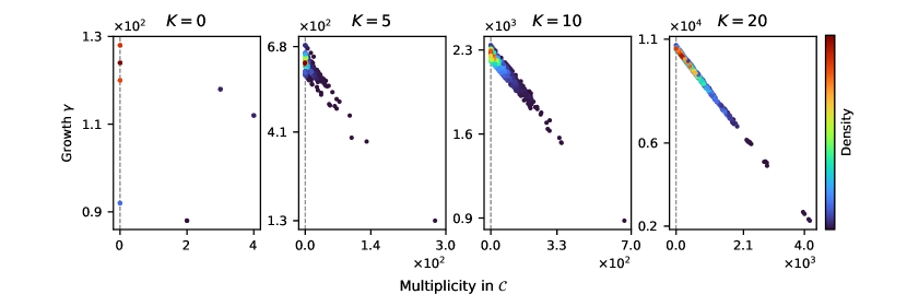
Figure 4: Comparison of multiplicity in $\mathcal{C}$ and growth incurred by Pauli products in the top gradient partition for various effective Hamiltonians along the GM($1$)-iQCC procedure applied to the CAS($6$e, $6$o) $N_{2}$ system at bond length $R=1.5$ Å in the cc-pVDZ basis. $K$ denotes the usage of the $K^{\rm{th}}$ iteration effective Hamiltonian, $\hat{H}^{(K)}$. For each plot, the multiplicities in $\mathcal{C}$ and growths for all $2^{N-1}=2048$ Pauli products in the top gradient partition of the Pauli pool for $\hat{H}^{(K)}$ are shown. Points in regions of greatest density are coloured red, e.g., $\hat{H}^{(0)}$ only has seven unique data points for all $2048$ Pauli products, with a dominating majority having zero multiplicity in $\mathcal{C}$.

B.0.2 Approximate probabilistic algorithm

Algorithm 2 Probabilistic variant of Algorithm 1.

Input $\mathcal{H}$, $\vec{\mu}^{(k)}$, $r$, $N_{\rm{samples}}$
      Output smallest growth element $\hat{P}_{\alpha}$ with gradient $g_{\alpha}$ and growth $\gamma^{(k)}$

1:obtain set $\bm{\mu}$

2:initiate $\mathcal{C}=\{\}$

3:initiate $\texttt{valid\_pairs}=\{\}$

4:for $\vec{\mu}^{(i)},\vec{\mu}^{(j)}\in\bm{\mu}$, $i<j$ do

5:     if $\vec{\mu}^{(i)}+\vec{\mu}^{(j)}\mod 2=\vec{\mu}^{(k)}$ then

6:         update $\texttt{valid\_pairs}\to\texttt{valid\_pairs}\cup\{(\vec{\mu}^{(i)},\vec{\mu}^{(j)})\}$

7:     end if

8:end for

9:for sample in $1,2,\ldots n_{\rm{samples}}$ do

10:     uniformly select $(\vec{\mu}^{(i)},\vec{\mu}^{(j)})\in\texttt{valid\_pairs}$

11:     uniformly select $\hat{Z}_{l}^{(i)}\in\mathcal{Z}_{i}$, $\hat{Z}_{l^{\prime}}^{(j)}\in\mathcal{Z}_{j}$

12:     compute $\hat{C}=[\hat{Z}_{l}^{(i)}\hat{X}_{i},\hat{Z}_{l^{{}^{\prime}}}^{(j)}\hat{X}_{j}]$

13:     if $\hat{C}\neq 0$ then

14:         update $\mathcal{C}\to\mathcal{C}+\{\hat{C}\}$

15:     end if

16:end for

17:count occurrences $m_{\mathcal{C}}(\hat{P}_{\alpha})$ for each unique $\hat{P}_{\alpha}\in\mathcal{C}$

18:for $r$ highest occurring $\hat{P}_{\alpha}\in\mathcal{C}$ do

19:     compute $|\mathcal{H}_{A}^{(\alpha)}|$

20:     compute and save $\gamma_{\alpha}=\left|[\hat{P}_{\alpha},\mathcal{H}]/\mathcal{H}_{A}^{(\alpha)}\right|$

21:end for

22:select $\hat{P}_{\alpha^{{}^{\prime}}}$ with smallest $\gamma_{\alpha^{{}^{\prime}}}$. Then $\gamma^{(k)}=\gamma_{\alpha^{{}^{\prime}}}$

For problem instances featuring large $M$, Algorithm 1 can be bottlenecked when computing $\mathcal{C}_{ij}$ for all valid $x$-string pairs. To alleviate time and memory requirements of this step, we propose a modified version of Algorithm 1 which utilizes uniform sampling. First, we uniformly sample valid $x$-string pairs, i.e. uniformly select which set we sample from in $\{\mathcal{C}_{ij}\}_{(ij)}$. Then, instead of computing the selected $\mathcal{C}_{ij}$ set exhaustively, we sample an element of $\mathcal{C}_{ij}$ by uniformly sampling $l$ and $l^{{}^{\prime}}$ (see Eq. (30)). The resulting commutator constitutes a “sample” and is saved if it is non-zero. Since generally growths are negatively correlated with multiplicities in $\bigcup_{(ij)}\mathcal{C}_{ij}$, and higher multiplicity elements are uniformly sampled from $\bigcup_{(ij)}\mathcal{C}_{ij}$ with higher probability (the probability of sampling a Pauli product $\hat{P}_{\alpha}$ is given by $\sum_{(ij)}m_{\mathcal{C}_{ij}}(\hat{P}_{\alpha})/|\sum_{(ij)}\mathcal{C}_{ij}|$), we find that this probabilistic variant of Algorithm 1 finds the lowest growth element with high success rate and with dramatically less resources. We found empirically that setting the number of samples to be a linear function of $M$ successfully finds the lowest growth element for systems studied in this work. Similarly to Algorithm 1, we then compute $|\mathcal{H}_{A}^{(k)}|$ for the $r$ most sampled Pauli products. However, we have not computed all of $\mathcal{C}$, rather we have only sampled elements from it $N_{\rm{samples}}$ times. Hence, the values of $m_{\mathcal{C}}(\hat{P}_{\alpha})$ are not readily available. Thus we compute $\gamma_{\alpha}$ as $\left|[\hat{P}_{\alpha},\mathcal{H}]/\mathcal{H}_{A}^{(\alpha)}\right|$. We summarize the probabilistic routine in Algorithm 2.

Table 3: A comparison of performance between the deterministic (“Det.”) and probabilistic (“Prob.”) minimum growth search algorithms of Algorithm 1 and Algorithm 2 respectively. For the probabilistic algorithm, $N_{\rm{samples}}=M$ was used. For all examples tabulated, $\gamma^{(k)}$ was obtained for the highest gradient. Observed $\gamma^{(k)}$ values for the probabilistic algorithm are the averages of the lowest growth values computed over ten runs, with standard deviations in brackets. For each effective Hamiltonian, all ten runs find the minimal growth element found in the deterministic algorithm, hence all standard deviations are zero.

Iteration	$M$	Algorithm	$N_{\rm{query}}$	Observed $\gamma^{(k)}$
$0$	$247$	Det.	$540$	$112$
		Prob.	$247$	$112.0(0.0)$
$5$	$1.24\times 10^{3}$	Det.	$1.37\times 10^{4}$	$130$
		Prob.	$1.24\times 10^{3}$	$130.0(0.0)$
$10$	$4.47\times 10^{3}$	Det.	$1.29\times 10^{5}$	$878$
		Prob.	$4.47\times 10^{3}$	$878.0(0.0)$
$20$	$2.10\times 10^{4}$	Det.	$1.99\times 10^{6}$	$2263$
		Prob.	$2.10\times 10^{4}$	$2263.0(0.0)$

A comparison between the deterministic and probabilistic algorithms is summarized in Table 3. Both algorithms were applied to the CAS($6$e, $6$o) $N_{2}$ system at bond length $R=1.5$ Å in the cc-pVDZ basis. Effective Hamiltonians at various iterations of the $s(1,0)$ iQCC procedure applied to this system were used for assessment. The number of Hamiltonian Pauli products with coefficient values with magnitude above $10^{-8}$ is denoted by $M$. The main cost of the algorithms is encapsulated by $N_{\rm{query}}$, which refers to the number of times the algorithm must query the commutator function between two Pauli products. Note that non-zero commutators are saved, hence time and memory requirements of both algorithms scale with $N_{\rm{query}}$. For both deterministic and probabilistic algorithms, $r=\lceil\log_{2}M\rceil$ was used. We observe that even for large scale effective Hamiltonians, setting $N_{\rm{samples}}=M$ in Algorithm 2 always finds the lowest growth element found in the deterministic approach of 1. This is significant, since in this case we query the commutator function between two Pauli products $N_{\rm{query}}=M$ times using Algorithm 2, versus $N_{\rm{query}}=O(M^{2})$ using Algorithm 1. In practice, we observe up to $\sim 100\times$ reductions in the number of commutator queries resulting in immensely reduced time and memory requirements, while maintaining identical performance in terms of the lowest observed growth element.

References

- Cao et al. [2019] Y. Cao, J. Romero, J. P. Olson, M. Degroote, P. D. Johnson, M. Kieferová, I. D. Kivlichan, T. Menke, B. Peropadre, N. P. D. Sawaya, S. Sim, L. Veis, and A. Aspuru-Guzik, Quantum chemistry in the age of quantum computing, Chem. Rev. 119, 10856 (2019).
- Bauer et al. [2020] B. Bauer, S. Bravyi, M. Motta, and G. K.-L. Chan, Quantum algorithms for quantum chemistry and quantum materials science, Chem. Rev. 120, 12685 (2020).
- Tilly et al. [2022] J. Tilly, H. Chen, S. Cao, D. Picozzi, K. Setia, Y. Li, E. Grant, L. Wossnig, I. Rungger, G. H. Booth, and J. Tennyson, The variational quantum eigensolver: A review of methods and best practices, Phys. Rep. 986, 1 (2022), the Variational Quantum Eigensolver: a review of methods and best practices.
- de Leon et al. [2021] N. P. de Leon, K. M. Itoh, D. Kim, K. K. Mehta, T. E. Northup, H. Paik, B. S. Palmer, N. Samarth, S. Sangtawesin, and D. W. Steuerman, Materials challenges and opportunities for quantum computing hardware, Science 372, eabb2823 (2021).
- Peruzzo et al. [2014] A. Peruzzo, J. McClean, P. Shadbolt, M.-H. Yung, X.-Q. Zhou, P. J. Love, A. Aspuru-Guzik, and J. L. O’Brien, A variational eigenvalue solver on a photonic quantum processor, Nat. Commun. 5, 4213 (2014).
- Hempel et al. [2018] C. Hempel, C. Maier, J. Romero, J. McClean, T. Monz, H. Shen, P. Jurcevic, B. P. Lanyon, P. Love, R. Babbush, A. Aspuru-Guzik, R. Blatt, and C. F. Roos, Quantum Chemistry Calculations on a Trapped-Ion Quantum Simulator, Phys. Rev. X 8, 31022 (2018).
- Romero et al. [2018] J. Romero, R. Babbush, J. R. McClean, C. Hempel, P. J. Love, and A. Aspuru-Guzik, Strategies for quantum computing molecular energies using the unitary coupled cluster ansatz, Quantum Sci. Technol. 4, 014008 (2018).
- Lee et al. [2019] J. Lee, W. J. Huggins, M. Head-Gordon, and K. B. Whaley, Generalized unitary coupled cluster wave functions for quantum computation, J. Chem. Theory Comput. 15, 311 (2019).
- Sokolov et al. [2020] I. O. Sokolov, P. K. Barkoutsos, P. J. Ollitrault, D. Greenberg, J. Rice, M. Pistoia, and I. Tavernelli, Quantum orbital-optimized unitary coupled cluster methods in the strongly correlated regime: Can quantum algorithms outperform their classical equivalents?, J. Chem. Phys. 152, 124107 (2020).
- Mizukami et al. [2020] W. Mizukami, K. Mitarai, Y. O. Nakagawa, T. Yamamoto, T. Yan, and Y.-y. Ohnishi, Orbital optimized unitary coupled cluster theory for quantum computer, Phys. Rev. Res. 2, 033421 (2020).
- Anand et al. [2022] A. Anand, P. Schleich, S. Alperin-Lea, P. W. K. Jensen, S. Sim, M. Díaz-Tinoco, J. S. Kottmann, M. Degroote, A. F. Izmaylov, and A. Aspuru-Guzik, A quantum computing view on unitary coupled cluster theory, Chem. Soc. Rev. 51, 1659 (2022).
- Grimsley et al. [2019] H. R. Grimsley, S. E. Economou, E. Barnes, and N. J. Mayhall, An adaptive variational algorithm for exact molecular simulations on a quantum computer, Nat. Commun. 10, 3007 (2019).
- Ryabinkin et al. [2018] I. G. Ryabinkin, T.-C. Yen, S. N. Genin, and A. F. Izmaylov, Qubit coupled cluster method: A systematic approach to quantum chemistry on a quantum computer, J. Chem. Theory Comput. 14, 6317 (2018).
- Tang et al. [2021] H. L. Tang, V. Shkolnikov, G. S. Barron, H. R. Grimsley, N. J. Mayhall, E. Barnes, and S. E. Economou, Qubit-adapt-vqe: An adaptive algorithm for constructing hardware-efficient ansätze on a quantum processor, PRX Quantum 2, 020310 (2021).
- Ryabinkin et al. [2020] I. G. Ryabinkin, R. A. Lang, S. N. Genin, and A. F. Izmaylov, Iterative qubit coupled cluster approach with efficient screening of generators, J. Chem. Theory Comput. 16, 1055 (2020).
- Yordanov et al. [2021] Y. S. Yordanov, V. Armaos, C. H. W. Barnes, and D. R. M. Arvidsson-Shukur, Qubit-excitation-based adaptive variational quantum eigensolver, Commun. Phys. 4, 228 (2021).
- Zhang et al. [2021] Z.-J. Zhang, T. H. Kyaw, J. S. Kottmann, M. Degroote, and A. Aspuru-Guzik, Mutual information-assisted adaptive variational quantum eigensolver, Quantum Sci. Technol. 6, 035001 (2021).
- Liu et al. [2021] J. Liu, Z. Li, and J. Yang, An efficient adaptive variational quantum solver of the schrödinger equation based on reduced density matrices, J. Chem. Phys. 154, 244112 (2021).
- Liu et al. [2022] J. Liu, Z. Li, and J. Yang, Reducing circuit depth in adaptive variational quantum algorithms via effective hamiltonian theories, J. Chem. Theory Comput. 18, 4795 (2022).
- Bauman et al. [2019] N. P. Bauman, E. J. Bylaska, S. Krishnamoorthy, G. H. Low, N. Wiebe, C. E. Granade, M. Roetteler, M. Troyer, and K. Kowalski, Downfolding of many-body hamiltonians using active-space models: Extension of the sub-system embedding sub-algebras approach to unitary coupled cluster formalisms, J. Chem. Phys. 151, 014107 (2019).
- Metcalf et al. [2020] M. Metcalf, N. P. Bauman, K. Kowalski, and W. A. de Jong, Resource-efficient chemistry on quantum computers with the variational quantum eigensolver and the double unitary coupled-cluster approach, J. Chem. Theory Comput. 16, 6165 (2020).
- Motta et al. [2020] M. Motta, T. P. Gujarati, J. E. Rice, A. Kumar, C. Masteran, J. A. Latone, E. Lee, E. F. Valeev, and T. Y. Takeshita, Quantum simulation of electronic structure with a transcorrelated hamiltonian: improved accuracy with a smaller footprint on the quantum computer, Phys. Chem. Chem. Phys. 22, 24270 (2020).
- Huang et al. [2023] R. Huang, C. Li, and F. A. Evangelista, Leveraging small-scale quantum computers with unitarily downfolded hamiltonians, PRX Quantum 4, 020313 (2023).
- Genin et al. [2022] S. N. Genin, I. G. Ryabinkin, N. R. Paisley, S. O. Whelan, M. G. Helander, and Z. M. Hudson, Estimating phosphorescent emission energies in iriii complexes using large-scale quantum computing simulations, Angew. Chem. Int. Ed. 61, e202116175 (2022).
- Ryabinkin et al. [2021] I. G. Ryabinkin, A. F. Izmaylov, and S. N. Genin, A posteriori corrections to the iterative qubit coupled cluster method to minimize the use of quantum resources in large-scale calculations, Quantum Sci. Technol. 6, 024012 (2021).
- McClean et al. [2020] J. R. McClean, N. C. Rubin, K. J. Sung, I. D. Kivlichan, X. Bonet-Monroig, Y. Cao, C. Dai, E. S. Fried, C. Gidney, B. Gimby, P. Gokhale, T. Häner, T. Hardikar, V. Havlíček, O. Higgott, C. Huang, J. Izaac, Z. Jiang, X. Liu, S. McArdle, M. Neeley, T. O’Brien, B. O’Gorman, I. Ozfidan, M. D. Radin, J. Romero, N. P. D. Sawaya, B. Senjean, K. Setia, S. Sim, D. S. Steiger, M. Steudtner, Q. Sun, W. Sun, D. Wang, F. Zhang, and R. Babbush, Openfermion: the electronic structure package for quantum computers, Quantum Sci. Technol. 5, 034014 (2020).
- Turney et al. [2012] J. M. Turney, A. C. Simmonett, R. M. Parrish, E. G. Hohenstein, F. A. Evangelista, J. T. Fermann, B. J. Mintz, L. A. Burns, J. J. Wilke, M. L. Abrams, N. J. Russ, M. L. Leininger, C. L. Janssen, E. T. Seidl, W. D. Allen, H. F. Schaefer, R. A. King, E. F. Valeev, C. D. Sherrill, and T. D. Crawford, Psi4: an open-source ab initio electronic structure program, WIREs Computational Molecular Science 2, 556 (2012).
- Kottmann et al. [2021] J. S. Kottmann, S. Alperin-Lea, T. Tamayo-Mendoza, A. Cervera-Lierta, C. Lavigne, T.-C. Yen, V. Verteletskyi, P. Schleich, A. Anand, M. Degroote, S. Chaney, M. Kesibi, N. G. Curnow, B. Solo, G. Tsilimigkounakis, C. Zendejas-Morales, A. F. Izmaylov, and A. Aspuru-Guzik, Tequila: a platform for rapid development of quantum algorithms, Quantum Sci. Technol. 6, 024009 (2021).
- Qiskit contributors [2023] Qiskit contributors, Qiskit: An open-source framework for quantum computing (2023).
- Barca et al. [2020] G. M. J. Barca, C. Bertoni, L. Carrington, D. Datta, N. De Silva, J. E. Deustua, D. G. Fedorov, J. R. Gour, A. O. Gunina, E. Guidez, T. Harville, S. Irle, J. Ivanic, K. Kowalski, S. S. Leang, H. Li, W. Li, J. J. Lutz, I. Magoulas, J. Mato, V. Mironov, H. Nakata, B. Q. Pham, P. Piecuch, D. Poole, S. R. Pruitt, A. P. Rendell, L. B. Roskop, K. Ruedenberg, T. Sattasathuchana, M. W. Schmidt, J. Shen, L. Slipchenko, M. Sosonkina, V. Sundriyal, A. Tiwari, J. L. Galvez Vallejo, B. Westheimer, M. Wloch, P. Xu, F. Zahariev, and M. S. Gordon, Recent developments in the general atomic and molecular electronic structure system, J. Chem. Phys. 152, 154102 (2020).
- McClean et al. [2018] J. R. McClean, S. Boixo, V. N. Smelyanskiy, R. Babbush, and H. Neven, Barren plateaus in quantum neural network training landscapes, Nat. Commun. 9, 1 (2018).