Symplectic mechanics of relativistic spinning compact bodies I.:
Covariant foundations and integrability around black holes

Abstract

In general relativity, the motion of an extended body moving in a given spacetime can be described by a particle on a (generally non-geodesic) worldline. In first approximation, this worldline is a geodesic of the underlying spacetime, and the resulting dynamics admit a covariant and 4-dimensional Hamiltonian formulation. In the case of a Kerr background spacetime, the Hamiltonian was shown to be integrable by B. Carter and the now eponymous constant. At the next level of approximation, the particle possesses proper rotation (hereafter spin), which couples the curvature of spacetime and drives the representative worldline away from geodesics. In this article, we lay the theoretical foundations of a series of works aiming at exploiting the Hamiltonian nature of the equations governing the motion of a spinning particle, at linear order in spin. Our formalism is covariant and 10-dimensional. It handles the degeneracies inherent to the local Lorentz invariance of general relativity with tools from Poisson geometry, and accounts for the center-of-mass/spin-supplementary-condition using constrained Hamiltonian system theory. As a first application, we consider the linear-in-spin motion in a Kerr background. We show that the resulting Hamiltonian system admits exactly five functionally independent integrals of motion related to Killing symmetries, thereby proving that the system is integrable. We conclude that linear-in-spin corrections to the geodesic motion do not break integrability, and that the resulting trajectories are not chaotic. We explain how this integrability feature can be used to reduce the computational cost of waveform generation schemes for asymmetric binary systems of compact objects.

Introduction

.1 The relativistic motion of test bodies

The last decades have seen both the advent of gravitational wave astronomy B. P. Abbott et al. (2016) (LIGO Scientific Collaboration and Virgo Collaboration); B. P. Abbott et al. (2019) (LIGO Scientific Collaboration and Virgo Collaboration); B. P. Abbott et al. (2020) (LIGO Scientific Collaboration and Virgo Collaboration); Abbott et al. (2021) and the first direct observations of a black hole’s strong field region Akiyama et al. (2019, 2022). These revolutionary events come as a reward for decades of effort in understanding the family of compact objects, namely black holes, neutron stars, and possibly exotic stars Cardoso et al. (2016); Toubiana et al. (2021). Of particular interest are binary systems of compact objects, which have been at the core of many still ongoing research programs, in view of the future of gravitational wave detectors on Earth Unnikrishnan (2013); Punturo et al. (2010) or in space Amaro-Seoane et al. (2017). Our ability to predict with great accuracy the motion of such systems directly impacts the likeliness of detecting them through their gravitational-wave emission. Thankfully, when it comes to the motion of compact binary systems under their mutual gravitational attraction, not all of their physical properties influence their motion the same way. This “universality” feature, unique to gravitation, is the main reason why multipolar expansions work: one models a real, extended compact object as a point particle endowed with a finite number of multipoles, e.g, mass, linear and angular momentum, deformability coefficients, etc. The higher the number of multipoles, the finer (and the closer to reality) the description of the object. The motion of the body is then obtained by solving a coupled problem: an equation of motion determining the wordline of the particle representing the body, and some evolution equations for the particle’s multipoles along that worldline. This very general result holds for any sufficiently compact object with a conserved stress-energy-momentum tensor Dixon (1974); Harte (2015).

For a small compact object moving in a given, background spacetime, the foundations of the multipolar schemes were laid in 1937 by Miron Mathisson. Key contributions were then made by Papapetrou in the forties, Tulzyjew in the fifties and culminated in the sixties with a series of articles by Dixon, essentially clarifying previous works and giving the “big picture.” We refer to Chap. 2 of Ramond (2021) for a detailed historical account and references for these pioneering works. The most modern and enlightening framework is undoubtedly that based on “generalized Killing fields”, developed by Harte Harte (2012, 2015, 2020). This approach sheds light on many uncovered aspects of previous derivations, makes explicit the difference between kinematical and dynamical effects, and is able to account for the self-fields of the body. The relevant evolution equations, now known as the Mathisson-Papapetrou-Tulczyjew-Dixon (MPTD) equations, are simple manifestations of the attempt to maintain Poincaré invariance as much as possible along the body’s representative worldline Harte (2008). These equations have been thoroughly studied and solved for a plethora of background spacetimes both theoretically and numerically, in particular exact and hairy black holes (see references below) and cosmological metrics Harte (2007); Obukhov and Puetzfeld (2011); Zalaquett et al. (2014). The MPTD equations are also recovered in the context of black hole perturbation theory Pound (2015); Miller and Pound (2021), making them not just “effective” equations replacing the extended body’s true motion, but a real sub-part of Einstein’s field equations.

.2 Relativistic Hamiltonian formulation

When the multipole description of the orbiting body is truncated at dipolar order, the MPTD system possesses two equations: one evolves a linear momentum 1-form $p_{a}$ and the other an antisymmetric spin tensor $S^{ab}$. Since the MPTD equations describes a purely kinematical evolution Harte (2015) of $p_{a},S^{ab}$, it is natural to look for a Hamiltonian formulation of these equations. In the case of general relativity, two distinct approaches have been proposed in the past. One of them is based on extending, to curved spacetime, the Lagrangian formulation of a free spinning particle in flat spacetime Hanson and Regge (1974). Inspired by this work and similar development in effective field theory Porto (2006), the authors of Barausse et al. (2009) provided a Hamiltonian formulation of the dipolar MPTD system via a singular Legendre transformation of this Lagrangian. Extensions to quadrupolar Vines et al. (2016) and octupolar orders Marsat (2015) have been derived, allowing for the SSC to be understood as a gauge freedom Steinhoff (2011). One drawback of these Lagrangian formulations, however, is their non-covariance, i.e., they require (i) a particular 3+1 split of the background spacetime and (ii) a fine-tuned choice of spin supplementary condition with no clear physical interpretation.

The other approach can be traced back to Souriau’s symplectic approach Souriau (1970) to the problem, cf. the recent note on Souriau’s pioneering ideas Damour (2024). While our treatment does not follow directly Souriau’s, it is solely based on symplectic geometry too, and borrow Souriau’s general philosophy: the Hamiltonian system will be considered the prime ingredient, and not a mere Legendre transform of some Lagrangian. The general symplectic structure that we shall use is already present (but somewhat hidden) in Souriau’s Souriau (1970) and Kunzle’s work Künzle (1972), but it seems that its first clear appearance is in d’Ambrosi et al. (2015) (see also references Witzany et al. (2019)). Naturally, our formulation will share some similarities with other covariant approaches proposed in d’Ambrosi et al. (2015, 2016); Witzany et al. (2019); Witzany (2019). However, the works d’Ambrosi et al. (2015, 2016) only work at the level of the equations of motion for simple orbits and do not exploit the Hamiltonian nature of the system. Similarly, the Hamiltonians proposed in Witzany et al. (2019); Witzany (2019) have a number of drawbacks that are unsatisfactory for practical applications, in particular ad-hoc mass parameters too many phase space dimensions, both issues related to unresolved constraints.Lastly, the necessary choice of spin supplementary condition for the well-posedness of the MPTD system will lead us, inevitably, to algebraic constraints. In the Lagrangian formalism, this is usually treated using the Dirac-Bergmann algorithm Barausse et al. (2009); Brown (2022). Here, in the context of symplectic geometry, this will be handled within the classical theory of “constrained Hamiltonian systems” following classical textbooks Arnold et al. (2006) (or Deriglazov (2022) for detailed proofs).

.3 The question of integrability around black holes

At monopolar order, the spin tensor $S^{ab}$ is not involved in the description of the body. The two MPTD equations reduce to (i) $p^{a}$ is parallel-transported along the worldline and (ii) $p^{a}$ is tangent to the worldline. Combining the two implies that the worldline is a geodesic of the background spacetime. The equations of geodesic motion are the most general setup to describe “free systems”, as was first realized by Arnold in Arnold (1966).Owing to their purely free (i.e., purely kinematical) evolution, such geodesic systems are usually simple enough that they can sometimes be integrable, i.e., possess enough integrals of motion that make the solution to their equations of motion solvable by quadrature (i.e., using algebraic manipulations and standard calculus). In general relativity, the most remarkable example of this is the integrability of geodesics in the Kerr spacetime, first demonstrated by Carter Carter (1968), five years after Kerr’s discovery of the eponymous metric describing rotating black holes Kerr (1963). Integrability of Kerr geodesics is far from trivial: there are not enough spacetime symmetries to produce enough constants of motion to ensure integrability. Interestingly, Carter’s proof actually relied on pure symplectic mechanics of the geodesic Hamiltonian, unaware of the existence of the existence of the Killing-Stäckel tensor while which only appeared two years later Walker and Penrose (1970).

While the integrability of the monopolar MPTD system (i.e., geodesics) around black holes is well understood Carter (1968); Frolov et al. (2017), its extension to the dipolar MPTD system (i.e., the motion of spinning particles) is not so clear. Based on existing numerical simulations exhibiting artefacts classically associated to chaos, it is reasonable to believe that the integrability of geodesics is generally broken by the effect of the body’s spin, in the Schwarzschild case Bombelli and Calzetta (1992); Verhaaren and Hirschmann (2010); Zelenka et al. (2020) as well as in Kerr Suzuki and Maeda (1997); Semerák (1999); Kyrian and Semerák (2007); Han (2008); Compère and Druart (2022). This seems to be the case for other types of (non-spin) perturbations, as explored in Witzany et al. (2015); Polcar et al. (2022); Mosna et al. (2022). However, when limiting to spin effect that are linear in $S^{ab}$, no clear answer exists in the literature. Our results fill this gap with an analytical proof of integrability (thus, no chaos arises at linear-in-spin order).

.4 Motivation and main results

In this work, our primary motivation lies in the fact that integrability (or lack thereof) for the motion of a small compact object around a black hole is directly related to the possibility of using gravitational self-force theory to build gravitational waveforms for extreme mass ratio inspiral (EMRI) systems Barack and Pound (2018); Pound and Wardell (2021), one of the primary sources of gravitational waves for Laser Interferometer Space Antenna (LISA) Amaro-Seoane et al. (2017). The Hamiltonian formulation of the equations governing EMRIs is currently of major interest in this particular field because it can account for most of the non-geodesic effects that require implementing to meet LISA’s accuracy requirements Afshordi et al. (2023). This includes the small body’s spin Boyle et al. (2008); Vines et al. (2016); Witzany et al. (2019); Lukes-Gerakopoulos and Witzany (2021), the conservative part of the gravitational self-force Vines and Flanagan (2015a); Fujita et al. (2017); Blanco and Flanagan (2023a) and possibly its dissipative sector too Galley (2013), while also being adapted to efficient and consistent numerical resolution schemes such as symplectic integrators Haier et al. (2006); Wang et al. (2021). In addition, if the Hamiltonian system is integrable, it can be written in terms of action-angle variables, which are Taylor-made for two-timescale expansion methods Hinderer and Flanagan (2008), gauge-invariant analysis of resonances Hinderer and Flanagan (2008), an elementary derivation of the first law of mechanics Isoyama et al. (2014); Le Tiec (2015) as well as flux-balance laws Isoyama et al. (2018); Grant and Moxon (2023a), all of which are invaluable tools used in the modeling and understanding of binary system mechanics. Spinning degrees of freedom of the secondary object are not yet fully implemented in state-of-the art results of EMRI waveform modeling, even though they are under heavy investigation Piovano et al. (2020); Mathews et al. (2022); Rahman and Bhattacharyya (2023). Our work contributes to this ongoing effort, in order to exploit future gravitational wave detectors at their full potential Barausse et al. (2020); Lukes-Gerakopoulos and Witzany (2021).

Our objective, through this series of work (of which this article is the first part), is to extend all the aforementioned results to the linear-in-spin, dipolar case. As they are strongly tied to Kerr geodesics being (i) Hamiltonian and (ii) integrable, our first aim is to (i) give a Hamiltonian formulation of the linear-in-spin dynamics and (ii) apply it the Kerr spacetime and show its integrability.

As argued above, various proposals have already been made for a Hamiltonian formulation of the dipolar MPTD system that only satisfies some of the criteria below. Our first main result is a formulation of the linear-in-spin MPTD system (9) as a Hamiltonian system that is at once:

• symplectic : it comes with a Poisson structure free of degeneracies

• a first integral : it is autonomous and not a pure phase space constraint,

• self-consistent : it does not keep terms of the same order in spin as it omits,

• covariant : it is independent of a choice of spacetime coordinates or tetrad field,

• 10-dimensional : as a simple counting of the independent degrees of freedom require,

Besides the formalism, a number of secondary formulae that may be useful in other contexts are given, and clarifications of various statements made in the literature are discussed.

The proof of integrability in the Schwarzschild and Kerr spacetimes relies on exhibiting enough functionally independent integrals of motion. Since our Hamiltonian formulation of the linear-in-spin, dipolar MPTD system is 10-dimensional, integrability follows from the existence of 5 such integrals, denoted $(\mu,E,L_{z},\mathfrak{K},\mathfrak{Q})$. All have a simple physical interpretation and are associated to some kind of symmetry:

• the mass $\mu$ of the body is conserved because the particle evolves freely at dipolar order (no self-induced force or torque from higher-order multipoles), its associated Killing structure is the metric $g_{ab}$, a particular Killing-Stäckel tensor,

• the particle’s total energy $E$, as measured at spatial infinity, is conserved thanks to the stationarity of the Kerr background, with associated timelike Killing vectors $(\partial_{t})^{a}$,

• the component $L_{z}$ of total angular momentum along the primary black hole’s spin axis, as measured at spatial infinity, is conserved thanks to the axisymmetry of the Kerr background, with associated spacelike Killing vector $(\partial_{\phi})^{a}$,

• two additional integrals $\mathfrak{K},\mathfrak{Q}$, known as Rüdiger’s invariants, are built from the hidden symmetry associated to a Killing-Yano tensor. While $\mathfrak{K}$ is the projection of the particle’s spin 4-vector onto the covariant angular momentum, $\mathfrak{Q}$ is a linear-in-spin generalization of the geodesic Carter constant.

We note that we did not discover any of these five integrals of motion: they have been known (at least) since Rüdiger’s work Rüdiger (1981, 1983) on linear-in-spin invariants of motion for the dipolar MPTD system. The novelty rather comes from the rigorous and covariant Hamiltonian setup in which they can be understood as functionally independent, first integrals, ensuring integrability.

.5 Organization of the paper

This article will serve as the basis for many extensions, starting with Ramond and Isoyama (2024), and contains detailed that will be otherwise omitted in further application-oriented publications. Everything is justified or proved as rigorously as possible. It is organized as follows.

• We start in Sec. I by reviewing the main aspects of the MPTD system, focusing on the dipolar order in Sec. I.1 and the important notion of “spin supplementary condition (SSC) for spinning particles in Sec. I.2. Our choice for the Tulczyjew-Dixon SSC is motivated in Sec. I.3 and the linear-in-spin dynamics are covered in Sec. I.4. The equations of interest for the rest of the article, are Eqs. (9) and (6) (hereafter “the system”).

• A first Hamiltonian formulation of the system is provided in Sec. II, where it is built on a 14-dimensional phase space, denoted $\mathcal{M}$, in Sec. II.1. Sections II.2 and II.3 contain the resulting equations of motion and an important change of coordinates, respectively. The phase space $\mathcal{M}$ is then reduced to a 12-dimensional one, denoted $\mathcal{N}$, by lifting the degeneracies on $\mathcal{M}$ associated to the local Lorentz invariance of general relativity, as explained in Sec. II.4.

• Section III is aimed at covering $\mathcal{N}$ with canonical coordinates, and discussing their physical meaning. The derivation, though technical and relegated to App. B, is based on a method that will be relevant for applications, namely transforming non-canonical coordinates into canonical ones. For an explicit example of its use, see Ramond and Isoyama (2024). A summary of the 12D formulation on $\mathcal{N}$ is then provided in Sec. III.3,

• Section IV is divided in two parts: first in Sec. IV.1 we rigorously incorporate the Tulczyjew-Dixon spin supplementary condition into the framework, thereby reducing the phase space once again, from $\mathcal{N}$ to a final 10-dimensional phase space $\mathcal{P}$ where all physical trajectories lie. The final formulation is summarized in Sec. IV.2 and is the first main result of this paper. Second, in Sec. IV.3, the state-of-the-art results for invariants of the MPTD system are discussed in the context of our Hamiltonian framework.

• Lastly, in Sec. V with apply the 10-dimensional formulation to the Schwarzschild and Kerr spacetime, in Sec. V.2 and Sec. V.3, respectively. All explicit formulae are given, and the proof of integrability follows from straightforward calculations of Poisson brackets on the 10-dimensional phase space $\mathcal{P}$. This section contains many explicit formulae on which subsequent works in this series will be based.

A concluding section Conclusions and prospects contains a summary of our results in Sec. Concluding summary and a number of possible applications and prospects in Sec. Future applications, most of which are already ongoing. All our notations and conventions for Lorentzian and symplectic geometry are described in App. A, and a Mathematica Companion Notebook, accessible by simple request, contains an explicit verification of all calculations made in Sec. V related to integrability in Kerr.

I Spinning point particles in general relativity

A sometimes overlooked, yet remarkable result of general relativity is that, if a compact object is moving in a given background spacetime (with no back reaction) and modeled as a point particle with (an arbitrarily large number of) multipoles, then its equations of motion can be found in closed form. Moreover, these equations have been derived in a variety of different and independent ways: multipolar expansion Tulczyjew (1959); Dixon (1974); Steinhoff and Puetzfeld (2010), Lagrangian formalism Steinhoff (2015a), gravitational self-force Gralla and Wald (2008); Pound (2012); Mathews et al. (2022), generalized Killing fields Harte (2012, 2015, 2020); see also Chap. 2 in Ramond (2021) for a survey of such methods. Here we only summarize the key results from this branch of relativistic mechanics.

We consider a fixed background spacetime $(\mathscr{E},g_{ab})$ where $\mathscr{E}$ is a 4-dimensional (4D) manifold covered with four coordinates $x^{\alpha}$, and $g_{ab}$ is a metric tensor on $\mathscr{E}$. The actual, physical trajectory of a compact object and all of its continuous, fluid-like properties can be put in correspondence with the worldline $\mathscr{L}\subset\mathscr{E}$ of a representative point particle endowed with multipoles, in a scheme often referred to as a multipolar skeleton formalism Dixon (2015); Harte (2015); Mathews et al. (2022). The higher the number of multipoles, the finer the description of the extended body by the multipolar particle. A whole hierarchy of multipoles enters the description at successive multipolar orders. For example, at monopolar order, the extended body is described by a particle endowed with a single monopole: its four-momentum vector $p^{a}$. At dipolar order, an antisymmetric, rank-2 spin tensor $S^{ab}$ is added on top of $p^{a}$, for a total of 10 degrees of freedom (4 translational ones in $p^{a}$ and 6 rotational ones in $S^{ab}$). Beyond the monopolar and dipolar order ($n=0$ and $n=1$ respectively), each multipolar order $n\geq 2$ adds a tensor of valence $n+2$ (called a $2^{n}$-pole) to the description of the body, bringing an additional $(n+3)(3n-1)$ independent degrees of freedom due to their algebraic symmetries Dixon (1974). These multipoles evolve along the worldline according to a system of ten coupled, ordinary differential equations (ODE) known as the Mathisson-Papapetrou-Tulczyjew-Dixon (MPTD) equations. They take the general form

$$(\nabla_{v}p)_{a} =R_{abcd}S^{bc}v^{d}+F_{a}\,,$$ (1a)

$$(\nabla_{v}S)^{ab} =2p^{[a}v^{b]}+N^{ab}\,,$$ (1b)

where $v^{a}$ is an arbitrary tangent vector to $\mathscr{L}$ and $\nabla_{v}:=v^{a}\nabla_{a}$ is the (metric-compatible) covariant derivative along $v^{a}$, $R_{abcd}$ is the Riemann curvature tensor of the background spacetime and $F_{a},N^{ab}$ denote contributions from higher-order multipoles coupled to the geometry, starting with the quadrupole. Note the absence of evolution equations for the quadrupole and higher-order multipoles. Much like in classical mechanics Harte (2015), the MPTD system is not sufficient to describe the system beyond the dipolar order. The quadrupole and other, higher-order multipoles need to be given in terms of $p^{a},S^{ab}$ and the geometry. These expressions are not universal, and can be found by examining the properties of black hole metrics and/or micro-physics for neutron and exotic stars (see for example references in Ramond and Le Tiec (2021)). Even with such models for the quadrupoles and higher-order multipoles, the system is still ill-posed, as there are more unknowns than equations. This comes from two observations. First, the tangent vector $v^{a}$ is arbitrary in (1) (i.e., not necessarily normalized) as the MPTD equations are actually invariant by re-parametrization of $\mathscr{L}$. From now, one we will set $v^{a}=u^{a}$, where $u^{a}$ is the four-velocity of the particle, normalized as $u_{a}u^{a}=-1$. Second, there is freedom in choosing the worldline that represents the body. At monopolar order, this is not an issue, but starting at dipolar order, this freedom requires a choice to define the angular momentum of the particle properly Steinhoff (2015a); Vines et al. (2016). This is discussed in more details in Sec. I.2.

I.1 The dipolar MPTD system

In the present work, we will truncate the MPTD system (1) at dipolar order, so that all the physical information about the compact object is encoded into a four-momentum form $p_{a}$ (not tangent to $\mathscr{L}$ in general) and an antisymmetric spin tensor $S^{ab}$. The dipolar MPTD system is obtained by turning off all beyond-dipolar-order multipoles Eqs. (1), which is equivalent to neglecting the force $F_{a}$ and torque $N^{ab}$ Harte (2015). One is left with the dipolar MPTD equations:

$$(\nabla_{u}p)_{a} =R_{abcd}S^{bc}u^{d}\,,$$ (2a)

$$(\nabla_{u}S)^{ab} =2p^{[a}u^{b]}\,.$$ (2b)

The physical interpretation of (2) is clear: the coupling between $S^{ab}$ and the background curvature $R_{abcd}$ drives the evolution of $p^{a}$, while the misalignment of $p^{a}:=g^{ab}p_{b}$ of $u^{a}$ drives the evolution of $S^{ab}$. Three scalar fields along $\mathscr{L}$ can be defined from the multipoles of the particle:

$$\mu^{2}:=-p_{a}p^{a}\,,\qquad S_{\circ}^{2}:=\frac{1}{2}S_{ab}S^{ab}\,,\quad\text{and}\quad S_{\star}^{2}:=\frac{1}{8}\varepsilon_{abcd}S^{ab}S^{cd}\,.$$ (3)

By assumption, $p^{a}$ is time like while $S^{ab}$ is spacelike, resulting in $\mu\geq 0$, $S_{\circ}\geq 0$ and $S_{\star}\geq 0$. Among these norms, $\mu$ and $S_{\circ}$ will be referred to as the mass, and $S_{\circ}$ as the spin norm. Note that they are intrinsically defined from the particle’s multipole, and do not depend on any observer. These quantities are, in general, not conserved under the dipolar MPTD system (2).

A remark of importance has to be made about Eqs. (2). It is known that the spin of any compact object will induce a quadratic-in-spin quadrupole Marsat (2015) (see also Chap. 6 in Ramond (2021)), which contributes to both force $F_{a}$ and torque $N^{ab}$ in the full MPTD system (1). Therefore, when truncating (1) at dipolar order to obtain (9), we have effectively neglected all quadratic-in-$S^{ab}$ contributions from the right-hand side of (1). Consequently, to remain self-consistent, Eqs. (9) would also need to be linearized in $S^{ab}$. If not, one would include quadratic-in-spin corrections from the dipolar sector but omits those of the quadrupolar sector, leading to inconsistency. Therefore, it should be kept in mind that the dipolar MPTD equations (2) are only self-consistent at linear order in spin. This linearization, rather ambiguous if the “spin” means the tensor $S^{ab}$, can be done properly with a choice of spin supplementary condition and the introduction of a spin-related, small parameter, as explained in Sec. I.4.

I.2 Spin supplementary conditions

The number of independent unknowns in $(v^{\alpha},p_{\alpha},S^{\alpha\beta})$ is $4+4+6=14$. Yet, there are only $10$ differential equations in (2). This ambiguity comes from an arbitrariness in the choice of parameter $\lambda$ associated to the tangent vector $v^{\alpha}$, and in the definition of the spin tensor, which contains angular momentum to be defined with respect to some reference (as in classical mechanics). A common way of fixing these issues (and thus having a well-posed differential system), is to 1) take $v^{a}=u^{a}$, the four-velocity along $\mathscr{L}$ so that $\lambda$ is the proper time $\tau$ and the condition $u^{a}u_{a}=-1$ reduces the number of unknowns to 13, and 2) impose a so-called spin supplementary condition (SSC), reducing this number to 10. An SSC takes the form of 3 algebraic constraints of the form

$$f_{a}S^{ab}=0\,,$$ (4)

where $f^{a}$ is some timelike vector defined along $\mathscr{L}$ (only three because this equation projected onto $f_{b}$ gives $0=0$ by antisymmetry of $S^{ab}$). To elucidate the meaning of such SSC, perform a Hodge decomposition of $S^{ab}$ with respect to the timelike vector $f^{a}$, effectively splitting $S^{ab}$ into a spin vector $S^{a}$ and mass dipole vector $D^{a}$, according to

$$S^{ab}=\varepsilon^{abcd}f_{c}S_{d}+2D^{[a}f^{b]}\quad\Leftrightarrow\quad\begin{cases}\,S^{b}=\frac{1}{2}\varepsilon^{abcd}f_{a}S_{cd}\,,\\ D^{b}=f_{a}S^{ab}\,.\end{cases}$$ (5)

The six degrees of freedom contained in the tensor $S^{ab}$ are encoded in the spacelike vectors $S^{a}$ and $D^{a}$, which have only three degrees of freedom each, as both verify the constraint of being orthogonal to $f^{a}$. Clearly, the SSC (4) means, physically, that the mass dipole $D^{a}$ measured in the spacelike frame of timelike direction $f^{a}$ vanishes. In that frame, $S^{ab}$ possesses three degrees of freedom and can be entirely described in terms of $S^{a}$. This decomposition is entirely analogous to the decomposition of the Faraday tensor $F^{ab}$ of electromagnetism into magnetic $B^{a}$ and electric $E^{a}$ fields measured by a given observer Gourgoulhon (2013), with the dictionary $(F^{ab},B^{a},E^{a})\leftrightarrow(S^{ab},S^{a},D^{a})$.

The natural question is: which frame should be chosen?, i.e., which vector $f^{a}$ in (4) ?. This question goes beyond the scope of the present work, and we refer to the thorough review Witzany et al. (2019) and references therein for details on the matter of SSCs (see also Lukes-Gerakopoulos et al. (2014); Costa and Natário (2015); Timogiannis et al. (2021)). While different choices of SSC will lead to more or less simple evolution equations, physical meaning and mathematical well-posedness, one generally expects that physical observables should all remain the same regardless of the chosen SSC, at least at dipolar order Steinhoff (2011, 2015b); Lukes-Gerakopoulos (2017).

I.3 The Tulzyjew-Dixon SSC

In this article and subsequent works, we shall work with the so-called Tulczyjew-Dixon spin supplementary condition (TD SSC) Tulczyjew (1959); Dixon (1964) :

$$C^{b}:=p_{a}S^{ab}=0\,.$$ (6)

Combining the TD SSC (6) with the dipolar MPTD equations (2) leads to a number of well-known results, recalled here for convenience. First, it follows from Eq. (2b) that the spin norm $S_{\circ}$ is constant along $\mathscr{L}$. Second, from (5), we find $S_{\star}=0$ (as enforced by any SSC Witzany et al. (2019)). Third, as shown first in Ehlers and Rudolph (1977) (see also Obukhov and Puetzfeld (2011) for a covariant proof), the TD SSC implies the following exact expression for the tangent vector $v^{a}$ in terms of $p_{a},S^{ab}$ and the background geometry

$$u^{a}=\frac{m}{\mu^{2}}\left(p^{a}+\frac{2S^{ab}R_{bcde}p^{c}S^{de}}{4\mu^{2}+R_{abcd}S^{ab}S^{cd}}\right)\,,$$ (7)

where $m:=-p_{a}u^{a}$ can be expressed in terms of solely ($p_{a},S^{ab},R_{abcd}$) by contracting Eq. (7) with $v_{a}$ and re-inserting the result. Equation (7) readily implies that all the scalars (3) are conserved.

The momentum-velocity relation (7) is a consequence of the dipolar MPTD system (2) and the SSC (4). One could ask if the converse result holds true, i.e., whether the momentum-velocity relation (7) and the dipolar MPTD together imply $p_{a}S^{ab}=0$. This is almost the case, for Eqs. (7) and (2) actually imply that $\nabla_{v}(p_{a}S^{ab})=0$, i.e., that the four-vector $p_{a}S^{ab}$ is parallel-transported along $\mathscr{L}$. This feature that has no major implication for solving the equations themselves. Yet, it must be handled with care in a Hamiltonian formulation of those same equations. This is discussed in Sec. IV.1. Our choice of SSC (6) is not random, but motivated by a number of reasons, detailed below:

• to our knowledge, it is the only one for which a unique center-of-mass-like worldline can be unambiguously defined for the actual extended body, and for which mathematical proofs of unicity exist Beiglböck (1967); Madore (1969); Schattner (1979a, b); Harte (2015). Other SSCs tend to correspond to a family of worldlines rather than a unique one Costa et al. (2012).

• it leads to a momentum-velocity relation that can be generalized to any multipolar order and can also account for the presence of electromagnetic fields Gralla et al. (2010). To our knowledge, this has never been shown for any other SSC.

• it naturally emerges when looking at the MPTD equations from the point of view of generalized Killing fields, the formalism developed by A. Harte Harte (2012, 2015) that goes beyond the test body assumption and takes into account self-field effects.

• several works, including Rüdiger (1981, 1983); Compère and Druart (2022); Compère et al. (2023), aimed at finding invariants of motion for the MPTD system beyond the geodesic limit. These works proved successful when relying on the TD SSC, and methods do not seem to generalize to other SSCs.

• in spacetimes admitting a Killing-Yano tensor, it leads to a covariant notion of angular momentum Dietz and Rüdiger (1981); Dietz and Rudiger (1982); Compère and Druart (2022), with well-behaved geodesic and Newtonian limits for black hole spacetimes Ramond and Isoyama (2024).

• it is compatible with a covariant Hamiltonian formulation. As pointed out in Witzany et al. (2019), the reason is that the TD SSC is “co-moving” Witzany et al. (2019), i.e., it relies on only the intrinsic properties of the body ($p_{a},S^{ab}$) and no background fields

• for such covariant Hamiltonian formulations, the TD SSC uniquely reduces the number of degrees of freedom by the largest amount Witzany et al. (2019). In a canonical setup, this corresponds to two phase space dimensions.

• as seen in Sec. IV, the TD SSC defines a phase-space sub-manifold $\mathcal{T}$ that is invariant under the flow of the free particle Hamiltonian (12). This is a key aspect of our covariant formulation.

• in a future publication, we shall demonstrate how the linear-in-spin, Hamiltonian formalism presented in this paper can be extended covariantly to the quadratic-in-spin case. We have only been able to do this with the use of the TD SSC.

I.4 Linear-in-spin dynamics under the TD SSC

For convenience, from now on, we take the tangent vector $v^{a}$ to be the four-velocity $u^{a}$ of the particle. The associated parameter along $\mathscr{L}$ is the proper time, denoted $\tau$. Inserting (7), into (2) then leads to a closed system of 10 equations for the ten independent components of the momenta $(p_{a},S^{ab})$. This system of equations, however, has a singular limit (observe the denominator in (7)). To make it explicit, we introduce the (only) dimensionless physical parameter at play: If $1/L^{2}$ is the typical curvature scale of the background spacetime, then Eq. (7) is well-behaved only in the limit where

$$\epsilon:=\frac{S_{\circ}}{\mu L}\lesssim 1\,.$$ (8)

For a generic extended body, the spin angular momentum $S_{\circ}$ scales as $\mu\ell$ where $\ell$ is the typical size of the body, leading to $\epsilon=\ell/L$. We recover the small parameter tied to multipolar expansions that lead to the MPTD equations Dixon (1974); Harte (2012); Ramond and Le Tiec (2021). In the particular case of a compact object (defined by $\ell\simeq\mu$) orbiting around black hole of mass $M$ (for which $L\simeq M$) one readily obtains $\epsilon=\mu/M$. Therefore, the MPTD equations are well-suited to capture the leading effect of the spin in the context of binary systems with asymmetric mass ratio (see the discussions in Witzany et al. (2019); Miller and Pound (2021)).

With the small parameter (8), we can now rigorously expand the dipolar MPTD system to linear order in spin, by (i) setting $S^{ab}=S_{\circ}\bar{S}^{ab}$, $p^{a}=\mu\bar{p}^{a}$ and $R_{abcd}=\bar{R}_{abcd}/L^{2}$, with barred quantities being dimensionless, (ii) inserting this into Eqs. (2) and (7) and (ii) neglecting any non-linearity in $\epsilon$. This leads to

$$p^{a} =\mu u^{a}\,,$$ (9a)

$$(\nabla_{u}p)_{a} =R_{abcd}S^{bc}u^{d}\,,$$ (9b)

$$(\nabla_{u}S)^{ab} =0\,.$$ (9c)

It is worth noting at this order, Eq. (9a) implies that $p^{a}$ is tangent to $\mathscr{L}$, just as in the non-spinning (geodesic) case. Moreover, Eq. (9c) implies that $S^{ab}$ is parallel-transported along $\mathscr{L}$, just as for a test spin. However, Eq. (9b) implies that $\mathscr{L}$ is not a geodesic of $(\mathscr{E},g_{ab})$ because of the spin-curvature coupling. It is tempting to interpret the right-hand side of Eq. (9b) as a “force”, as it drives the evolution of the momentum. But we stress that there is no dynamical evolution in these equations. In fact, the MPTD system at dipolar order (2) is (i) pure kinematics: body-dependent multipoles only enter at quadrupolar order, with non-zero $F^{a},N^{ab}$ Harte (2015); Harte and Dwyer (2023); and (ii) completely universal: all spinning bodies with the same initial conditions will follow the same trajectories.

System (9) along with the TD SSC (6) is the system that we will to study in this paper. More precisely, what we will investigate in subsequent sections is the Hamiltonian formulation of the differential system given by the components of Eq. (9) onto the natural basis $(\partial_{\alpha})^{a}$ associated to some coordinate system $x^{\alpha}$ on $(\mathscr{E})$. This is the object of Sec. II. We also have to keep in mind that the well-posedness of Eqs. (9) relies on the TD SSC (6), which has to holds along $\mathscr{L}$. We will ensure that the latter is correctly incorporated into the Hamiltonian formulation in Sec. (IV). Lastly, we emphasize that all calculations, from now on, will be performed consistently at linear order in spin, and what we is meant by that, is that in any equation we can restore the dimensionless, small parameter $\epsilon$ (define in (8)) and neglect any non-linearity in $\epsilon$.

II The MPTD equations as a constrained Poisson system

In this section, we examine the linear-in-spin MPTD system (9) and write it as a Poisson system, a particular type of Hamiltonian systems which comes with degeneracies. (See App. (105) for details about different types of Hamiltonian systems.) First, the Poisson system is rigorously defined in Sec. II.1 and the resulting equations of motion are derived in Sec. II.2. Using a change of phase space coordinates in Sec. II.3, the Poisson system is shown to be degenerate (non-symplectic) in Sec. II.4, and the degeneracies are lifted accordingly.

II.1 Definition of the Poisson system

It is well-known that the linearized MPTD + TD SSC system (9) can be written as a Poisson system d’Ambrosi et al. (2015); Witzany et al. (2019). As reviewed in App. D, this type of system is constructed from three ingredients: a phase space $\mathcal{M}$, a Poisson structure $\Lambda$ on $\mathcal{M}$ (or, equivalently, a set of Poisson brackets $\{,\}$), and a Hamiltonian $H$.

II.1.1 Phase space

In the 4-dimensional spacetime manifold $(\mathscr{E},g_{ab})$, consider a coordinate system $x^{\alpha}$ and the natural bases $(\partial_{\alpha})^{a}$ and $(\mathrm{d}x^{\alpha})_{a}$ associated to it. Let the components of the four-momentum and spin tensor in these bases be $p_{\alpha}$ and $S^{\alpha\beta}$, respectively, and let $x^{\alpha}(\bar{\tau}$ be a parametrization of the dipolar particle’s worldline $\mathscr{L}$ with respect to the parameter $\bar{\tau}:=\tau/\mu$, which is affine parameter as $\mu$ is constant along $\mathscr{L}$. We then define a 14-dimensional phase space $\mathcal{M}=\mathbb{R}^{14}$, endowed with 14 phase space coordinates denoted

$$(x^{\alpha},p_{\beta},S^{\gamma\delta})\in\mathbb{R}^{4}\times\mathbb{R}^{4}\times\mathbb{R}^{6}\,,$$ (10)

such that their physical meaning is the one presented above. Note that changing the coordinates on $\mathscr{E}$ corresponds to a different covering of phase space coordinates, not just in $x^{\alpha}$, but also in $(p_{\alpha},S^{\beta\gamma})$ because of the natural bases used for their definition.

II.1.2 Poisson structure

The Poisson structure $\Lambda$ can be equivalently defined by a set of Poisson brackets between the coordinates (10), cf. App. D.2 for a summary of Poisson systems. There is a well-known set of such brackets in the context of the MPTD equations, see the references in Witzany et al. (2019). The non-vanishing ones are given explicitly by

$$\{x^{\alpha},p_{\beta}\} =\delta^{\alpha}_{\beta}\,,$$ (11a)

$$\{p_{\alpha},p_{\beta}\} =R_{\alpha\gamma\delta\beta}S^{\gamma\delta}\,,$$ (11b)

$$\{p_{\alpha},S^{\beta\gamma}\} =\Gamma^{\beta}_{\delta\alpha}S^{\delta\gamma}+\Gamma^{\gamma}_{\delta\alpha}S^{\beta\delta}\,,$$ (11c)

$$\{S^{\alpha\beta},S^{\gamma\delta}\} =g^{\alpha\gamma}S^{\beta\delta}-g^{\alpha\delta}S^{\beta\gamma}+g^{\beta\delta}S^{\alpha\gamma}-g^{\beta\gamma}S^{\alpha\delta}\,,$$ (11d)

where $\Gamma^{\alpha}_{\beta\gamma}$ are the Christoffel symbols associated to the metric $g_{ab}$, and $R_{\alpha\beta\gamma\delta}$ the components of the Riemann tensor in the natural basis. We stress that, in the phase space context, all GR geometric objects $g_{\alpha\beta},\Gamma^{\alpha}_{\beta\gamma},R_{\alpha\beta\gamma\delta},\ldots$ are viewed as simple functions of the coordinates $x^{\alpha}$. Formulae (11) determine a well-defined set of Poisson brackets, as they satisfy the two requirements to be so: anti-symmetry and the Jacobi identity, as discussed in App. C.2. While the anti-symmetry is easily checked, the Jacobi identity (104b) is verified in App. C.2 using the more practical coordinates defined in Sec. II.3.

II.1.3 Hamiltonian function

The last ingredient is a Hamiltonian function that will generate the same differential system as the MPTD equations. In Witzany et al. (2019), the authors derived a Hamiltonian for each of the commonly used SSC using heuristic arguments, essentially, because no clear strategy exists to do this in general. In that article, one can find (see Eq. (44) there) a Hamiltonian that generates both the (nonlinear) dipolar MPTD equations (2) and the TD momentum-velocity relation (7). However, this Hamiltonian is not well-suited for our purposes for several reasons. First, it is “pure constraint”, i.e., it vanishes identically on the sub-manifold defined by the TD SSC. This poses a problem when applying the Liouville-Arnold theorem Arnold et al. (2006) to discuss integrability, since the Hamiltonian itself cannot be used as an integral of motion. Second, the proposed Hamiltonian is valid under the assumption that the dynamical mass $\mu^{2}=-p_{a}p^{a}$ is a given parameter (independent of the phase space). This is unfortunate as (i) we will need it to find enough invariants of motion, and (ii) we expect the constancy of $\mu$ to be a natural consequence of the evolution equations (i.e., Hamilton’s equation, in this context) and not as a ad hoc condition. Third, they were built to generate the nonlinear dipolar MPTD system, and, therefore, contain too much information for our purposes, as already explained in Sec. I.1. Lastly, and perhaps most importantly, this Hamiltonian does not convey the central idea that at dipolar order, the MPTD equations are those of a test particle free of any finite size effect Harte (2012, 2015), or, equivalently, simple conservation laws associated to the local Lorentz invariance of general relativity Harte and Dwyer (2023). The dipolar particle is “free”, in the sense that equations (2) are universal (i.e., any body described at dipolar level satisfies these equations, whether it be a grain of dust, a planet or a compact object), with body-specific multipoles starting only at quadrupolar order Harte (2020). In particular, the spin-curvature coupling term in (2a) is not a general relativistic effect per-se: it already exists in the free particle motion of Newtonian mechanics in non-Euclidean spaces Arnold et al. (2006); Harte (2015). Based on these considerations, we vouch for a more natural choice, that of the free particle Hamiltonian

$$H:(x^{\alpha},p_{\alpha},S^{\alpha\beta})\mapsto\frac{1}{2}g^{\alpha\beta}p_{\alpha}p_{\beta}\,,$$ (12)

where, in terms of phase space variables, $g^{\alpha\beta}$ are functions of $x^{\alpha}$. Even though it has the same expression, this Hamiltonian is not, strictly speaking, the Hamiltonian that generates geodesics in the metric $g_{ab}$ (used for example in Schmidt (2002)). Indeed, even though it does not depend explicitly on $S^{\alpha\beta}$, it is still considered a function of $(x^{\alpha},p_{\alpha},S^{\alpha\beta})$. The equations of motion will, therefore, still contain terms involving the spin because of the Poisson structure (11).

II.2 Equations of motion

The computation of the equations of motion is made with respect to some arbitrary parameter $\lambda$ along the worldline (the “time” conjugated to the Hamiltonian), using the (generalized) Hamilton equations:

$$\frac{\mathrm{d}F}{\mathrm{d}\lambda}=\{F,H\}=\{F,x^{\alpha}\}\,\frac{\partial H}{\partial x^{\alpha}}+\{F,p_{\alpha}\}\,\frac{\partial H}{\partial p_{\alpha}}+\{F,S^{\alpha\beta}\}\,\frac{\partial H}{\partial S^{\alpha\beta}}\,,$$ (13)

with $F$ any function of the phase space variables. To be precise, in Eq. (13) the first equality is a definition (that of the evolution of $F:\mathcal{M}\rightarrow\mathbb{R}$ under the flow of $H$ for the Poisson system $(\mathcal{M},\{,\},H)$), and the second equality makes use of the Leibniz rule satisfied by the Poisson bracket. The evolution parameter $\lambda$ is that uniquely conjugated to the Hamiltonian (such that $\{\lambda,H\}=1$). It can be physically interpreted only once we compare the Hamilton equations to the system (9).

The partial derivatives of the Hamiltonian (12) are easily found to be

$$\frac{\partial H}{\partial x^{\alpha}}=-\Gamma^{\gamma}_{\alpha\beta}p_{\gamma}p^{\beta}\,,\quad\frac{\partial H}{\partial p_{\alpha}}=g^{\alpha\beta}p_{\beta}\quad\text{and}\quad\frac{\partial H}{\partial S^{\alpha\beta}}=0\,,$$ (14)

where we projected the metric compatibility condition $\nabla_{a}g_{bc}=0$ onto the natural basis to get the first equation. We then replace $F$ in Eq. (13) by the phase space coordinates $x^{\alpha},p_{\alpha},S^{\alpha\beta}$ and combine Eqs. (11), (13) and (14) to obtain the evolution for each coordinate:

$$w^{\alpha}:=\frac{\mathrm{d}x^{\alpha}}{\mathrm{d}\lambda} =g^{\alpha\beta}p_{\beta}\,,$$ (15a)

$$\frac{\mathrm{d}p_{\alpha}}{\mathrm{d}\lambda} =\Gamma^{\nu}_{\alpha\lambda}p_{\nu}w^{\lambda}-\frac{1}{2}R_{\alpha\beta\mu\nu}S^{\mu\nu}w^{\beta}\,,$$ (15b)

$$\frac{\mathrm{d}S^{\alpha\beta}}{\mathrm{d}\lambda} =-(\Gamma^{\alpha}_{\lambda\nu}S^{\lambda\beta}+\Gamma^{\beta}_{\lambda\nu}S^{\alpha\lambda})w^{\nu}\,,$$ (15c)

where $w^{\alpha}$ is just a notation for $\mathrm{d}x^{\alpha}/\mathrm{d}\lambda$. Regarding Eqs. (15b) and (15c), the first term on their right-hand side can be absorbed into their left-hand side by introducing covariant derivatives $\nabla_{w}=w^{\alpha}\nabla_{\alpha}$. We note that Eqs. (15b) and (15c) are exactly the linearized MPTD equations at dipolar order (9), written with respect to tangent vector $w^{\alpha}=p^{\alpha}$. Therefore, the parameter $\lambda$ uniquely associated to the Hamiltonian (12) corresponds physically to the worldline parameter associated to $p^{a}$ as a tangent vector to $\mathscr{L}$. By virtue of Eq. (9a), we find $\lambda:=\bar{\tau}=\tau/\mu$, and we shall use $\bar{\tau}$ from now on. We note that this is the same result as in the non-spinning, geodesic case. Since $\mu$ is conserved along $\mathscr{L}$, physically speaking, $\bar{\tau}$ is an affine parameter.

II.3 Alternative coordinates

The phase space coordinates (10) are useful to prove that the Hamiltonian system (12)-(11) is equivalent to the original system (9). It is also relevant for interpretation purposes. However, when it comes to reducing the system and to doing Hamiltonian mechanics per-se, they are not practical at all. Here, we introduce a new system of coordinates on $\mathcal{M}$ which still retains some physical intelligibility while also admitting drastically simpler Poisson brackets.

First, we require some geometrical construction within spacetime $(\mathscr{E},g_{ab})$. Consider an orthonormal tetrad field $\{(e_{A})^{a}\}_{A\in\{0,\ldots,3\}}$, whose components in the natural basis are $(e_{A})^{\alpha}$ ($A$ labels the four different vectors, and $\alpha$ the four components of the $A$-th vector). Let $\omega_{aBC}:=g_{bc}(e_{B})^{b}\nabla_{a}(e_{C})^{c}$ be the connection 1-forms associated to the tetrad. Since $\omega_{aBC}=-\omega_{aCB}$, there are six independent such 1-forms. Their components in the natural basis, $\omega_{\alpha BC}$, are the connection coefficients and those in the tetrad, $\omega_{ABC}$, are the so-called Ricci rotation coefficients (we follow Sec. 3.4b of Wald (1984)). As before, all these objects are defined throughout spacetime, and become simple functions of the phase space coordinates $x^{\alpha}$ in the phase space picture. New coordinates on $\mathcal{M}$ are then obtained by (i) keeping the coordinates $x^{\alpha}$, (ii) replacing the linear momentum variables $p_{\alpha}$ by $\pi_{\alpha}$, a combination of linear and angular momentum, and (iii) replacing $S^{\alpha\beta}$ by $S^{AB}$, the tetrad components of the spin tensor. Explicitly, we define these new coordinates $(x^{\alpha},\pi_{\alpha},S^{AB})$ by setting

$$p_{\alpha} =\pi_{\alpha}+\frac{1}{2}\omega_{\alpha BC}S^{BC}\,.$$ (16a)

$$S^{\alpha\beta} =S^{AB}(e_{A})^{\alpha}(e_{B})^{\beta}\,.$$ (16b)

Solving these equations for $\pi_{\alpha}$ and $S^{AB}$ shows that this coordinate change is indeed invertible, and takes the form $(x^{\alpha},p_{\alpha},S^{\alpha\beta})\mapsto(x^{\alpha},\pi_{\alpha}(z,p,S),S^{\alpha\beta}(z,S))$ where the right-hand side emphasizes the new coordinates’ dependence on the old set (10), denoted schematically by $(z,p,S)$. The Poisson brackets of the new coordinates can then be computed from the rule (103) and the old brackets (11). This calculation does not appear in the literature, to our knowledge. Therefore, we have detailed it in App. C. It is lengthy but straightforward, using not so well-known formulae involving the connection 1-forms (in particular Eq. (3.4.20) of Wald (1984)). The non-vanishing Poisson brackets are found to be:

$$\{x^{\alpha},\pi_{\beta}\} =\delta^{\alpha}_{\beta}\,,$$ (17a)

$$\{S^{AB},S^{CD}\} =2\eta^{A[D}S^{C]B}+2\eta^{B[C}S^{D]A}\,.$$ (17b)

Note that, even though the six $S^{AB}$ do not verify the canonical Poisson brackets, the four pairs $(x^{\alpha},\pi_{\alpha})$ do, and have vanishing Poisson brackets with $S^{AB}$. The spin variables $S^{AB}$ have Poisson brackets akin to the commutators of the so(1,3) algebra (see, e.g., Chap. 7 in Gourgoulhon (2013)). This is reminiscent of the definition of $S^{AB}$ as the components in an orthonormal tetrad field, the latter forming a set left invariant by the SO(1,3) group of Lorentz transformations. This property is even more clear when we use, instead of the six independent $S^{AB}$, the $3+3$ variables $(S^{1},S^{2},S^{3},D^{1},D^{2},D^{3})$ defined by

$$S^{I}=\frac{1}{2}\varepsilon^{I}_{\phantom{I}JK}S^{JK}\quad\text{and}\quad D^{I}=S^{0I}\,.$$ (18)

where $\varepsilon^{IJ}_{\phantom{IJ}K}$ is the 3D Levi-Civita symbol, equal to $1$ (resp. $-1$) when $IJK$ is an even (resp. odd) permutation of $123$, and $0$ otherwise. Although they are but notations in phase space, $S^{I}$ and $D^{I}$ have a clear physical meaning: they are the tetrad components of the Euclidean spin and mass dipole vectors as defined in Eq. (5) (i.e., with $(e_{0})^{a}$ replacing $f^{a}$ there). The brackets (17b), with these notations, take their simplest form

$$\{x^{\alpha},\pi_{\beta}\} =\delta^{\alpha}_{\beta}\,,$$ (19a)

$$\{S^{I},S^{J}\} =\varepsilon^{IJ}_{\phantom{IJ}K}S^{K}\,,$$ (19b)

$$\{D^{I},D^{J}\} =-\varepsilon^{IJ}_{\phantom{IJ}K}S^{K}\,,$$ (19c)

$$\{D^{I},S^{J}\} =\varepsilon^{IJ}_{\phantom{IJ}K}D^{K}\,.$$ (19d)

Now the brackets (19) are identical to the commutators of the generators for the Lie algebra so(1,3). We also stress that brackets (19) are equivalent to, it is more a renaming of the spin coordinates (through Eq. (18)) than a coordinate transformation.

We can now express the original Hamiltonian (12) in terms of the new coordinates $(x^{\alpha},\pi_{\beta},S^{I},D^{J})$ on $\mathcal{M}$, by inserting Eqs. (16) into Eq. (12). We obtain

$$H:(x^{\alpha},\pi_{\beta},S^{I},D^{J})\mapsto\frac{1}{2}g^{\alpha\beta}\pi_{\alpha}\pi_{\beta}+\frac{1}{2}g^{\alpha\beta}\pi_{\alpha}\omega_{\beta CD}S^{CD}\,.$$ (20)

Even though (20) calls for a rather natural identification into a “non-spinning” term $\tfrac{1}{2}g^{\alpha\beta}\pi_{\alpha}\pi_{\beta}$ corrected by a “linear-in-spin term” $\tfrac{1}{2}g^{\alpha\beta}\pi_{\alpha}\omega_{\beta CD}S^{CD}$. This split, however, should be interpreted with care, as there are spin-related quantities hidden in $\pi_{\alpha}$, cf. Eq. (16). We will always avoid any such interpretation, and rather treat the whole Hamiltonian as one describing an object with both linear and angular momentum (orbital and spin) intertwined.

II.4 Degeneracies of the Poisson structure

We now focus on the Poisson brackets (19) between the new coordinates $(x^{\alpha},\pi_{\alpha},S^{I},D^{I})$. Following the notations of App. D.2, we are in the case $N=14$ and we construct the Poisson matrix $\Lambda^{ij}(y)=\{y^{i},y^{j}\}$, where $(y^{1},\ldots,y^{14})$ denote the coordinates $(x^{\alpha},\pi_{\beta},S^{I},D^{I})$, in that order.

II.4.1 Rank

Directly reading through Eqs. (19), we find that the matrix $\Lambda$ is block diagonal, and given by

$$\Lambda=\left(\begin{array}[]{ll}\mathbb{J}_{8}&0\mathbb{}\\ 0&\mathfrak{S}\end{array}\right)\,,\quad\text{with}\quad\mathbb{J}_{8}=\left(\begin{array}[]{cc}0&\mathbb{I}_{4}\\ -\mathbb{I}_{4}&0\end{array}\right)\,,\quad\mathfrak{S}=\left(\begin{array}[]{cc}\mathcal{S}&\mathcal{D}\\ \mathcal{D}&-\mathcal{S}\end{array}\right)\,.$$ (21)

In the above equations, $\mathbb{I}_{4}$ it the $4\times 4$ identity matrix, so that $\mathbb{J}_{8}$ is the canonical $8\times 8$ Poisson matrix (it would be the Poisson matrix of four pairs of canonical coordinates in an 8-dimensional symplectic system), while $\mathfrak{S}$ is a $6\times 6$ antisymmetric matrix constructed from two SO(3) matrices associated to $S^{I}$ and $D^{I}$, namely

$$\mathcal{S}=\left(\begin{array}[]{ccc}0&S^{3}&-S^{2}\\ -S^{3}&0&S^{1}\\ S^{2}&-S^{1}&0\\ \end{array}\right)\quad\text{and}\quad\mathcal{D}=\left(\begin{array}[]{ccc}0&D^{3}&-D^{2}\\ -D^{3}&0&D^{1}\\ D^{2}&-D^{1}&0\\ \end{array}\right)\,.$$ (22)

The matrix formulation of the Poisson structure $\Lambda$ permits an easy calculation of its rank at each point of $\mathcal{M}$. Direct inspection reveals that $\text{rank}(\mathbb{J}_{8})=8$, while $\text{det}(\mathfrak{S})=0$ and $\text{det}(\mathfrak{S})=4$. Since $\Lambda=\text{diag}(\mathbb{J}_{8},\mathfrak{S})$, we obtain

$$\text{rank}(\Lambda)=12<14=\text{dim}(\mathcal{M})\,.$$ (23)

Therefore, as explained in Sec. D.2, the Poisson structure generated by the brackets of the coordinates (19), is degenerate. Consequently, there exists exactly $\text{dim}(\mathcal{M})-\text{rank}(\Lambda)=14-12=2$ Casimir invariants for this structure. We note that, since the rank (and the vanishing of the determinant) are invariant under diffeomorphisms, these feature (degeneracy and existence of two Casimirs) also hold for the initial brackets (11).

II.4.2 Casimirs

The brackets (19) admit two independent Casimir invariants, which can be explicitly computed. Following tradition Witzany et al. (2019), we shall take

$$\mathcal{C}_{\circ}:=\vec{S}\cdot\vec{S}-\vec{D}\cdot\vec{D}\quad\text{and}\quad\mathcal{C}_{\star}:=\vec{S}\cdot\vec{D}\,,$$ (24)

where we have used the Euclidean notations $\vec{S}=(S^{1},S^{2},S^{3})$ and $\vec{D}=(D^{1},D^{2},D^{3})$. We can verify directly with the brackets (19) and the Leibniz rule that they are Casimirs, i.e., that for any $(z,\pi,S,D)$-dependent function $F$, $\{F,\mathcal{C}_{\circ}\}=0$ and $\{F,\mathcal{C}_{\star}\}=0$, or we can also check that their gradient is in the null space of the Poisson matrix $\Lambda$. Either calculation is easily done and shows, indeed, that (24) are Casimirs. From a physical point of view, these quantities are easily interpreted: re-writing Eqs. (24) in terms of the variables $S^{AB}$, we obtain

$$\mathcal{C}_{\circ}=\frac{1}{2}\eta_{AB}\eta_{CD}S^{AC}S^{BD}\quad\text{and}\quad\mathcal{C}_{\star}=\frac{1}{8}\varepsilon_{ABCD}S^{AB}S^{CD}\,.$$ (25)

Most remarkably, Eqs. (25) coincide with the covariant definition Eqs. (3) expanded in an orthonormal tetrad. Therefore, the (phase space) Casimirs are numerically equal to the (squares of the) covariant spin norms:

$$\mathcal{C}_{\circ}=S_{\circ}^{2}\quad\text{and}\quad\mathcal{C}_{\star}=S_{\star}^{2}\,,$$ (26)

justifying the notation of the Casimirs. This result should be understood with care. The Poisson structure defined by the brackets (19) (or (11) equivalentmy) automatically implies the conservation of both spin norms $S_{\circ}^{2},S_{\star}^{2}$, as these are Casimirs $(\mathcal{C}_{\circ},\mathcal{C}_{\star})$ of the structure. As pointed out in Witzany et al. (2019), these spin scalars are not constant along the worldline $\mathscr{L}$ for the general MPTD system, but they are conserved the dipolar MPTD system with the TD SSC (regardless of linearization in spin). Indeed, $p_{a}S^{ab}=0$ readily implies $\nabla_{u}(S_{\circ})=0$ from Eq. (2b) and $S_{\star}=0$ from Eq. (5).

II.4.3 Symplectic leaves

As reviewed in App. D.2, even though the Poisson brackets (19) define a degenerate structure on the 14-dimensional manifold $\mathcal{M}$, the latter is foliated by so called “symplectic leaves”, which we denote by $\mathcal{N}$, and defined as the level sets of the Casimirs. Let us, therefore, set both Casimirs invariants (24) to some fixed values (naturally denoted by $S^{2}_{\circ},S^{2}_{\star}$), and consider the 12-dimensional sub-manifold $\mathcal{N}$ defined by the two independent algebraic equations

$$\mathcal{C}_{\circ}(z,\pi,S,D)=S_{\circ}^{2}\quad\text{and}\quad\mathcal{C}_{\star}(z,\pi,S,D)=S_{\star}^{2}\,,$$ (27)

where we have emphasized that these relations are really algebraic constraints between the coordinates $(z,\pi,S,D)$ on $\mathcal{M}$. The manifold $\mathcal{N}$ is symplectic (non-degenerate), and can be, at least in principle and locally, endowed with canonical coordinates. We shall see in Sec. (III) that such canonical coordinates can be found, and cover $\mathcal{N}$ globally. These coordinates hold for a given leaf $\mathcal{N}$. It thus expected that they are parametrized by the Casimirs values $S_{\circ},S_{\star}$. This is exactly what we shall find. In particular, on $\mathcal{N}$, $S_{\circ},S_{\star}$ are pure parameters, and not functions of the phase space coordinates, as they were on $\mathcal{M}$. This is important because it makes a distinction between several kinds of invariants of motion: Casimirs (for Poisson system, constant for any Hamiltonian) and first integrals (for symplectic systems, Hamiltonian-dependent). This distinction is important, in particular when counting the “integrals of motion” to check whether a Hamiltonian system is integrable or not.

Lastly, let us discuss the choice of Poisson structure on a given 12D leaf $\mathcal{N}$. Since the latter is defined as the subset of $\mathcal{M}$ where both Casimirs (24) are constant, we are in the presence of a constrained Hamiltonian system, with Eqs. (24) defining 2 constraints. Using the standard theory of constrained systems (reviewed in App. B), it follows that the Poisson structure $\Lambda^{\mathcal{N}}$ on $\mathcal{N}$ is the restriction of $\Lambda$ to $\mathcal{N}$. In generality, $\Lambda$ and $\Lambda^{\mathcal{N}}$ will be associated to different Poisson brackets $\{,\}\neq\{,\}^{\mathcal{N}}$. We will encounter this in section IV, where this difference is explicit in Eq. (43). However, when (and only when) the constraints correspond to Casimir invariants, a classical result of Poisson system theory Deriglazov (2022) shows that $\Lambda^{\mathcal{N}}$ and $\Lambda$ are essentially identical (this can be traced back to the Casimirs commuting with anything on $\mathcal{M}$). Therefore, the 7D Hamiltonian system $(\mathcal{M},\Lambda,H)$, when restricted to a given leaf $\mathcal{N}$, becomes the 6D Hamiltonian system ($\mathcal{N},\Lambda,H_{\mathcal{N}})$, where $\mathcal{N}$ is endowed with any (invertible) subset of 12 coordinates from $(x^{\alpha},\pi_{\alpha},S^{I},D^{I})$, and $H_{\mathcal{N}}$ is expressed in terms of these 12 coordinates. However, the original brackets (19) can still be used to evolve the system on $\mathcal{N}$, i.e., $\{F,G\}^{\mathcal{N}}=\{F,G\}$ for any functions $F,G$ on $\mathcal{N}$. In practice, it much more practical to derive 12 canonical coordinates on $\mathcal{N}$, instead of picking an arbitrary set of 12 from those on $\mathcal{M}$. From now on, no distinction will be made between $\{,\}$ and $\{F,G\}^{\mathcal{N}}$, and a Hamiltonian $H$ on $\mathcal{M}$ will still be denoted $H$ on $\mathcal{N}$, with the assumption that the number of variables on which it depends (14 or 12, respectively) leverage any risk of confusion.

III Canonical coordinates on $\mathcal{N}$

In this section, we provide explicit formulae relating the spin tensor tetrad components $S^{AB}$ to two symplectic pairs of variables $(\sigma,\pi_{\sigma}),(\zeta,\pi_{\zeta})$, and the two Casimir invariants (25). These variables, which are canonical pairs on any leaf $\mathcal{N}$, are defined in Sec. III.1 and their construction is relegated to App. B. We discuss their physical significance in Sec. III.2 and summarize the 12D canonical formulation on $\mathcal{N}$ in Sec. IV, emphasizing on its covariance.

III.1 Statement of the result

Since the 12D leaves $\mathcal{N}$ are symplectic (non-degenerate), it is tempting to try and construct 12 canonical coordinates, i.e., 6 pairs $(q^{i},p_{i})_{i\in\{1,\ldots,6\}}$ for which the brackets on $\mathcal{N}$ satisfy $\{q^{i},p_{j}\}=\delta^{i}_{j}$. To derive these coordinates, we note that the Casimirs (24) are only functions of $(S^{I},D^{I})$ and not $(x^{\alpha},\pi_{\alpha})$. A natural method to construct canonical coordinates on $\mathcal{N}$ emerges naturally: (i) keep the 4 pairs $(x^{\alpha},\pi_{\alpha})$ of $\mathcal{M}$, as they will be automatically canonical on $\mathcal{N}$, from Eq. (19a) (recall that $\{x^{\alpha},\pi_{\beta}\}^{\mathcal{N}}=\{x^{\alpha},\pi_{\beta}\}$), and (ii) construct 2 other canonical pairs covering the spin sector $(\vec{S},\vec{D})$, say $(\sigma,\pi_{\sigma}),(\zeta,\pi_{\zeta})$. The latter can be found by solving the nine spin-dependent brackets (17), now seen as canonical brackets on $\mathcal{N}$ of the 6 $(\sigma,\pi_{\sigma},\zeta,\pi_{\zeta})$-dependent functions $(S^{I},D^{I})$. For example, the bracket $\{S^{1},S^{2}\}=S^{3}$ on $\mathcal{M}$ now becomes a partial differential equation (PDE)

$$\frac{\partial S^{1}}{\partial\sigma}\frac{\partial S^{2}}{\partial{\pi_{\sigma}}}-\frac{\partial S^{2}}{\partial\sigma}\frac{\partial S^{1}}{\partial{\pi_{\sigma}}}+\frac{\partial S^{1}}{\partial\zeta}\frac{\partial S^{2}}{\partial{\pi_{\zeta}}}-\frac{\partial S^{2}}{\partial\zeta}\frac{\partial S^{1}}{\partial{\pi_{\zeta}}}=S^{3}\,,$$ (28)

in which $S^{1},S^{2},S^{3}$ are viewed as functions on $\mathcal{N}$ of the coordinates $(\sigma,\pi_{\sigma}),(\zeta,\pi_{\zeta})$. This calculation is rather non-trivial because the nine Poisson brackets turn into a system of nine nonlinear coupled PDEs, but educated guesses from the so(1,3) symmetries make things manageable.

III.1.1 Formulae

At the end of the aforementioned calculation, detailed in App. B, a remarkably simple solution of the PDE system is found. It reads

$$S^{1} =X\cos\sigma\,,$$ (29a)

$$S^{2} =X\sin\sigma\,,$$ (29b)

$$S^{3} =\pi_{\sigma}\,,$$ (29c)

$$D^{1} =Y\pi_{\sigma}\sin\zeta\cos\sigma+Y\pi_{\zeta}\cos\zeta\sin\sigma+XZ\cos\sigma\,,$$ (29d)

$$D^{2} =Y\pi_{\sigma}\sin\zeta\sin\sigma-Y\pi_{\zeta}\cos\zeta\cos\sigma+XZ\sin\sigma\,,$$ (29e)

$$D^{3} =-XY\sin\zeta+Z\pi_{\sigma}\,,$$ (29f)

where $X,Y,Z$ are functions of the momenta $(\pi_{\sigma},\pi_{\zeta})$ and the Casimir invariants $(S_{\circ},S_{\star})$, given by

$$X:=\sqrt{\pi_{\zeta}^{2}-\pi_{\sigma}^{2}}\,,\quad Y:=\sqrt{1-\frac{S_{\circ}^{2}}{\pi_{\zeta}^{2}}-\frac{S_{\star}^{4}}{\pi_{\zeta}^{4}}}\,,\quad Z:=\frac{S_{\star}^{2}}{\pi_{\zeta}^{2}}\,.$$ (30)

By construction, the pairs $(\sigma,\pi_{\sigma})$ and $(\zeta,\pi_{\zeta})$ are symplectic, i.e., their only non-vanishing Poisson brackets are $\{\sigma,\pi_{\sigma}\}=1$ and $\{\zeta,\pi_{\zeta}\}=1$.

III.1.2 Domain of definition

From direct inspection of Eqs. (29), we can take both $\sigma$ and $\zeta$ in the interval $[0,2\pi]$ without loss of generality. Moreover, all expressions are well-defined provided that $\pi_{\zeta}^{2}-\pi_{\sigma}^{2}\geq 0$ and $\pi_{\zeta}^{4}-S_{\circ}^{2}\pi_{\zeta}^{2}-S_{\star}^{4}\geq 0$. The first condition is straightforward, and the latter implies that ${\pi_{\zeta}}$ must be in the domain $]-\infty,-\Pi]\,\cup\,[\Pi,+\infty[$, where

$$\Pi=\sqrt{\frac{S_{\circ}^{2}}{2}+\frac{\sqrt{S_{\circ}^{4}+4S_{\star}^{4}}}{2}}\geq 0\,.$$ (31)

Note that one can simply take ${\pi_{\zeta}}\geq 0$ without loss of generality, since all expressions in (29) are invariant under ${\pi_{\zeta}}\mapsto-{\pi_{\zeta}}$, except for $D^{1}$ and $D^{2}$. But since $D^{1}(\sigma,{\pi_{\sigma}},\zeta,-{\pi_{\zeta}})=D^{1}(\sigma,{\pi_{\sigma}},\pi-\zeta,{\pi_{\zeta}})$, the choice ${\pi_{\zeta}}\geq 0$ is not restrictive to parametrize the phase space by $(\sigma,\zeta)\in[0,2\pi]\times[0,2\pi]$ and $({\pi_{\zeta}},{\pi_{\sigma}})\in\Delta$, where $\Delta\subset\mathbb{R}^{2}$ is the open set depicted in Fig. 1.

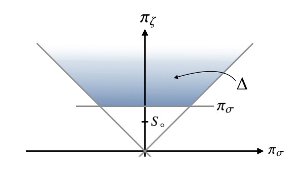
Figure 1: The open domain of definition $\Delta\subset\mathbb{R}^{2}$ for the canonical spin momenta $({\pi_{\sigma}},{\pi_{\zeta}})$.

III.1.3 Simplification under an SSC

When the TD spin supplementary condition is imposed, we shall see in Sec. IV that the Casimir $\mathcal{C_{\star}}=S_{\star}^{2}$ automatically vanishes. From Eq. (30), this implies $Z=0$ in Eqs. (29), making these formulae much simpler. The vanishing of $S_{\star}$ is actually independent of the particular choice of SSC, i.e., any timelike vector $f^{a}$ in (4) will readily enforce $S_{\star}=0$, as shown in Witzany et al. (2019).

As can be seen on Eqs. (29), an SSC will not enforce that the mass dipole $D^{I}\neq 0$ will vanish, even though when $S_{\star}=0$. This is because there is no unique mass dipole, but one for each observer, cf. the discussion in Sec. I.2. However, since $S_{\star}^{2}=\vec{S}\cdot\vec{D}$ (cf. Eq. (24)) the Euclidean 3-vectors $\vec{S}$ and $\vec{D}$ will be orthogonal (with respect to the Euclidean scalar product) under any SSC, for an observer on a worldline with timelike tangent vector $(e_{0})^{a}$. This gives an general interpretation of whether an SSC has been applied at all, independently of the particular choice (i.e., true for any $f^{a}$ in Eq. (4)).

III.2 Physical interpretation

The canonical coordinates (29) parametrizing a generic spin tensor $S^{AB}$ are, to the best of our knowledge, not discussed in the literature. This is particularly surprising since this the variables $S^{AB}$ satisfy the Lorentz so(1,3) algebra, probably the most important one of modern theoretical physics. In view of applications of the formalism presented in this paper to the case of black hole spacetimes, it is important to know what these coordinate represent physically. In the case of the Schwarzschild spacetime, this interpretation was crucial to construct other adapted coordinates via canonical transformations Ramond and Isoyama (2024).

Let us place ourselves in the reference frame defined by the tetrad $(e_{A})^{a}$, and imagine the three spatial legs as axes of a Cartesian coordinate system. Inspecting the first three equations in (29) shows that ${\pi_{\zeta}}$ is the norm of the Euclidean spin vector $\vec{S}$, and ${\pi_{\sigma}}$ is its projection onto the $\vec{e}_{3}$-axis. Moreover, $\sigma$ is the angle measured between $\vec{e}_{1}$ and the projection of $\vec{S}$ onto the plane Span$(\vec{e}_{1},\vec{e}_{2})$. Notably, in this Cartesian interpretation $((\pi_{\zeta}^{2}-\pi_{\sigma}^{2})^{1/2},\sigma,{\pi_{\sigma}})$ are the usual cylindrical coordinates of the vector $\vec{S}$. This is, of course, reminiscent of the SO(3)-like Poisson brackets verified by the spin vector; cf. Eq. (19b). Turning to the angle $\zeta$, we see that it parametrizes only the mass dipole $\vec{D}$. To elucidate its physical meaning, let us first note that, as given in Eqs. (29), both 3-vectors $\vec{S}$ and $\vec{D}$ clearly undergo a spatial rotation of angle $\sigma$ with respect to the $\vec{e}_{3}$-axis. Indeed, we can write

$$\vec{S}=\mathcal{R}_{\sigma}\vec{V}\,,\quad\vec{D}=\mathcal{R}_{\sigma}(Z\vec{V}+Y\vec{W})\quad\text{where}\quad\mathcal{R}_{\sigma}=\begin{pmatrix}\cos\sigma&-\sin\sigma&0\\ \sin\sigma&\cos\sigma&0\\ 0&0&1\end{pmatrix}\,,$$ (32)

and we have introduced two 3-vectors by their coordinates in the $(\vec{e}_{I})$ frame as $\vec{V}=((\pi_{\zeta}^{2}-\pi_{\sigma}^{2})^{1/2},0,{\pi_{\sigma}})$ and $\vec{W}=({\pi_{\sigma}}\sin\sigma,{\pi_{\zeta}}\cos\sigma,-(\pi_{\zeta}^{2}-\pi_{\sigma}^{2})^{1/2}\sin\sigma)$. By construction, $\vec{V}$ and $\vec{W}$ are orthogonal for the Euclidean scalar product. Therefore, the expression for $\vec{D}$ in (32) is the parallel-perpendicular decomposition of $\vec{D}$ with respect to $\vec{S}$, in the frame $(\vec{e}_{1}\phantom{}^{\prime},\vec{e}_{2}\phantom{}^{\prime},\vec{e}_{3})$ obtained by rotating $(\vec{e}_{1},\vec{e}_{2},\vec{e}_{3})$ by an angle $\sigma$ around the third axis. The angle $\zeta$ is then simply that which gives the direction of the perpendicular part of $\vec{D}$, as measured from the $\vec{e}_{2}\phantom{}^{\prime}$-axis. This is illustrated in Fig. 2.

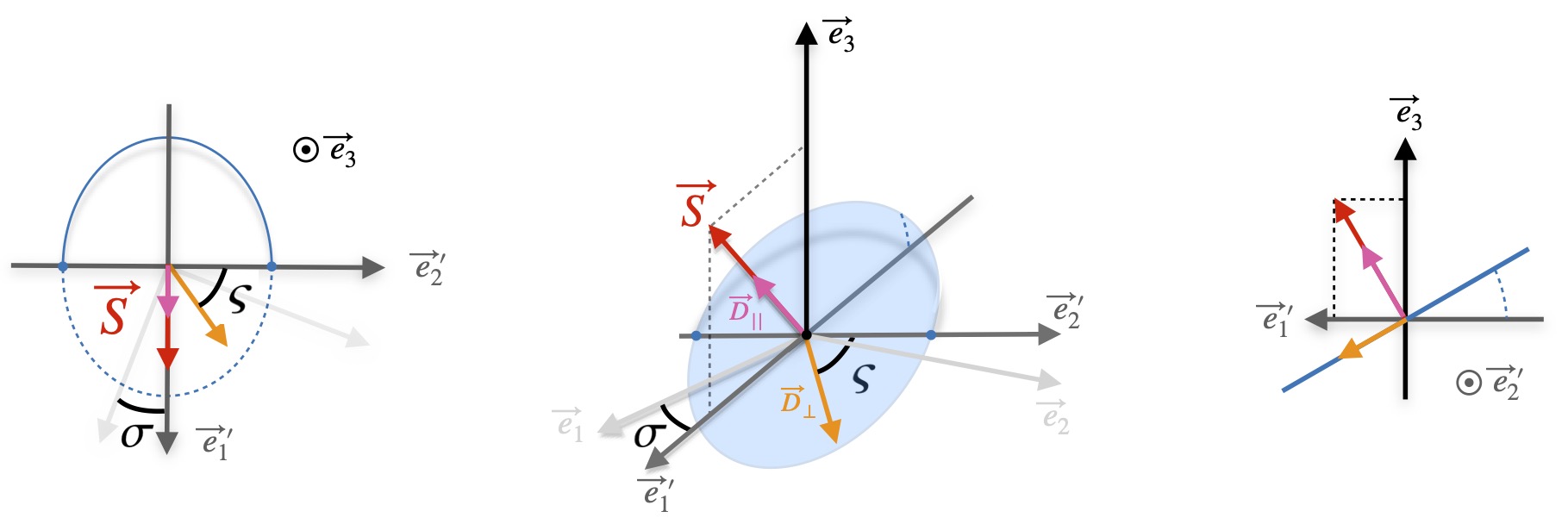
Figure 2: Physical interpretation of the symplectic variables $(\sigma,{\pi_{\sigma}},\zeta,{\pi_{\zeta}})$ in the 3-dimensional euclidean subspace $(\vec{e}_{1},\vec{e}_{2},\vec{e}_{3})$.

If there is an SSC, then $S_{\star}^{2}=\vec{D}\cdot\vec{S}=0$ (as argued in the last section) and, therefore, the parallel part of $\vec{D}$ vanishes. Hence, with any SSC the mass dipole $\vec{D}$ is purely orthogonal to $\vec{S}$ and given by the orange vector in Fig. 2. In addition, under any SSC, formulae (29) can be even more simplified by noting that ${\pi_{\sigma}}/{\pi_{\zeta}}\in[0,1]$. By introducing an angle $\chi$ such that $\cos\chi={\pi_{\sigma}}/{\pi_{\zeta}}$, Eqs. (29) become

$$S^{1} ={\pi_{\zeta}}\sin\chi\cos\sigma\,,$$ (33a)

$$S^{2} ={\pi_{\zeta}}\sin\chi\sin\sigma\,,$$ (33b)

$$S^{3} ={\pi_{\zeta}}\cos\chi\,,$$ (33c)

$$D^{1} =\sqrt{\pi_{\zeta}^{2}-S_{\circ}^{2}}\bigl{(}\cos\chi\sin\zeta\cos\sigma+\cos\zeta\sin\sigma\bigr{)}\,,$$ (33d)

$$D^{2} =\sqrt{\pi_{\zeta}^{2}-S_{\circ}^{2}}\bigl{(}\cos\chi\sin\zeta\sin\sigma-\cos\zeta\cos\sigma\bigr{)}\,,$$ (33e)

$$D^{3} =-\sqrt{\pi_{\zeta}^{2}-S_{\circ}^{2}}\sin\chi\sin\zeta\,.$$ (33f)

These formulae clearly show that $\vec{S}$ and $\vec{D}$ are two vectors of (Euclidean) norm ${\pi_{\zeta}}$ and $(\pi_{\zeta}^{2}-S_{\circ}^{2})^{1/2}$, respectively, along with some rotation parametrized by the angles $\sigma,\chi,\zeta$. In fact, if $\mathcal{R}_{I}(\alpha)$ denotes the $3\times 3$ matrix of a rotation of angle $\alpha$ with respect to the axis $\vec{e}_{I}$, then Eqs. (33) can be put into the compact form

$$\vec{S}={\pi_{\zeta}}\mathcal{R}_{3}(\sigma)\mathcal{R}_{2}(\chi)\vec{e}_{3}\quad\text{and}\quad\vec{D}=\sqrt{\pi_{\zeta}^{2}-S_{\circ}^{2}}\mathcal{R}_{3}(\sigma)\mathcal{R}_{2}(\chi)\mathcal{R}_{3}(\zeta)\vec{e}_{2}\,.$$ (34)

Equations (34), along with the relation $\cos\chi=\pi_{\sigma}/\pi_{\zeta}$, are equivalent to Eqs. (33), with the advantage of making all aforementioned properties particularly clear: norms of $\vec{S}$ and $\vec{V}$, interpretation of the angles ($\sigma,\zeta)$ and orthogonality properties. In addition, equation (34) that $(\sigma,\zeta,\chi)$, are the 3-2-3 Euler-angle parameterization Heard (2008) of $\vec{D}$ (and of $\vec{S}$ with $\zeta=0$), in the spatial triad $(e_{I})^{a}$. In particular, the momentum $\pi_{\zeta}$ is the norm of the spin 3-vector $\vec{S}$ in that frame, therefore, $\pi_{\zeta}\neq 0$ and Eqs. (29)–(30) are all well-posed.

III.3 Summary: 12D, covariant, non-degenerate formulation on $\mathcal{N}$

To summarize, at this stage the Hamiltonian system $(\mathcal{N},\Lambda,H)$ that we are considering is made of (i) the 12D phase space $\mathcal{N}$; (ii) the 6 pairs of canonical coordinates $(x^{\alpha},\sigma,\zeta,\pi_{\alpha},\pi_{\sigma},\pi_{\zeta})$ and (iii) the Hamiltonian obtained by inserting Eq. (16) into Eq. (12), namely

$$H(x^{\alpha},\sigma,\zeta,\pi_{\alpha},\pi_{\sigma},\pi_{\zeta})=\frac{1}{2}g^{\alpha\beta}\pi_{\alpha}\pi_{\beta}+\frac{1}{2}g^{\alpha\beta}\pi_{\alpha}\omega_{\beta CD}S^{CD}\,,$$ (35)

where $x^{\alpha}$ are hidden in $g^{\alpha\beta}$ and $\omega_{\beta CD}$, $\pi_{\alpha}$ appear explicitly, and the four spin variables $(\sigma,\pi_{\sigma},\zeta,\pi_{\zeta})$ are hidden in $S^{CD}$ through formulae (29). We emphasize that the Casimirs/spin norms $S_{\circ},S_{\star}$ are fixed parameters in the formulation (not phase space functions), and that the particle’s mass $\mu$ is the conserved value of the Hamiltonian itself along any solution to Hamilton’s equations. trajectory

This formulation is “covariant” in the sense that expression (35) holds for any choice of spacetime coordinates and any choice of background tetrad. To see why, perform a change of coordinates $x^{\alpha}\mapsto\tilde{x}^{\alpha}$ on the spacetime $(\mathscr{E},g_{ab})$. It naturally induces a change $x^{\alpha}(\bar{\tau})\mapsto\tilde{x}(\bar{\tau}^{\alpha}$ in the worldline’s parameterization spacetime. In general, the new coordinates $\tilde{x}^{\alpha}$ will not be canonically conjugated to the old momenta $\pi_{\alpha}$. However, consider the new momenta $\tilde{\pi}^{\alpha}(z,\pi)$ such that

$$\frac{\partial\tilde{\pi}_{\beta}}{\partial\pi_{\gamma}}\frac{\partial\tilde{x}^{\alpha}}{\partial x^{\gamma}}=\delta^{\alpha}_{\beta}\,.$$ (36)

Then, from the Leibniz rule, $\{\tilde{x}^{\alpha},\tilde{\pi}_{\alpha}\}=\delta^{\alpha}_{\beta}$, and the new pairs $(\tilde{x}^{\alpha},\tilde{\pi}_{\beta})$ are conjugated. In addition, the metric components $g^{\alpha\beta}$ and the connection 1-form components $\omega_{\alpha BC}$ change according to the usual chain rule characterizing tensors, and the whole expression in (35) is seen to be invariant under the change of spacetime coordinates.

Similarly, suppose a different tetrad (say $(\tilde{e}_{A})^{a}$ instead of $(e_{A})^{a}$) is chosen for the definition of the spin components $S^{AB}$ and the Ricci coefficients. Since, $(e_{A})^{a}$ and $(\tilde{e}_{A})^{a}$ are orthonormal tetrads, therefore, $(e_{B})^{a}=L^{A}_{\phantom{A}B}(\tilde{e}_{A})^{a}$, where $L^{A}_{\phantom{A}B}$ is an arbitrary Lorentz transformation. Then, a direct calculation from their definition shows that the 1-form component $\omega_{\beta CD}$ becomes $L^{A}_{\phantom{A}C}L^{B}_{\phantom{B}D}\tilde{\omega}_{\alpha AB}$, while the spin components in the new tetrad are $\bar{S}^{CD}=L^{C}_{\phantom{C}A}L^{D}_{\phantom{D}B}S^{AB}$. Therefore, since of a Lorentz transformation verifies $\eta_{AB}L^{A}_{\phantom{A}C}L^{B}_{\phantom{B}D}=\eta_{CD}$ by definition, we obtain $\omega_{\beta CD}S^{CD}=\tilde{\omega}_{\beta CD}\tilde{S}^{CD}$, and the expression (35) is left unchanged, as claimed.

IV Constraints and invariants

We have reduced the Hamiltonian formulation on the initial 14D phase space $\mathcal{M}$ to a 12D leaf $\mathcal{N}$ with no degeneracies. However, recall that the number of independent unknowns in the linearized MPTD + TD SSC system is 10 and not 12, cf. Sec. 9. In this section, we implement the TD SSC into the formulation on $\mathcal{N}$ (cf. the summary in Sec. III.3) by treating it as Hamiltonian constraints. This is done in Sec. IV.1, resulting in a 10D phase space, denoted $\mathcal{P}$, wherein our final result is formulated, as summarized in Sec. IV.2. Lastly, the link between invariants of the MPTD system and integrals of motion of our 10D Hamiltonian formulation is discussed in Sec. IV.3.

IV.1 Algebraic constraints from the TD SSC

The Hamiltonian system we are considering is described by the Hamiltonian (35) and the TD SSC in the form $p_{\alpha}S^{\alpha\beta}=0$. From a phase space point of view, the TD SSC is a set of four algebraic equations relating the 12 canonical phase space variables on $\mathcal{N}$ (or the 14 non-canonical variables of $\mathcal{M}$, equivalently). Therefore, we are in the presence of a constrained Hamiltonian system. We will now explain how to incorporate these constraints onto $\mathcal{N}$, thus reducing the number of phase space dimensions, and restricting to the only part of $\mathcal{N}$ where the physically well-defined trajectories lie.

First, we write the TD SSC in terms of the canonical variables on $\mathcal{N}$. Projecting Eq. (6) onto the tetrad, the TD SSC generates the following four algebraic equations

$$C^{B}(z,\pi,S,D):=\pi_{A}S^{AB}=0\,,$$ (37)

where, $\pi_{A}:=(e_{A})^{\alpha}\pi_{\alpha}$ is a function of $(x^{\alpha},\pi_{\alpha})$, and $S^{AB}$ is, as always, a function of $(\sigma,\pi_{\sigma},\zeta,\pi_{\zeta})$ via Eqs. (18) and (29). Now let $\mathcal{T}$ be the sub-manifold of $\mathcal{N}$ defined by the four algebraic equations (37), and let us explore its properties.

IV.1.1 Invariance and dimension of ${\mathcal{T}}$

First, we show that $\mathcal{T}$ is invariant under the flow of the Hamiltonian (35). Indeed, one can establish using the Leibniz rule and the brackets (17) that

$$\frac{\mathrm{d}C^{A}}{\mathrm{d}\lambda}=\{C^{A},H\}=\Omega^{A}_{\phantom{A}B}C^{B}\,,\quad\text{where}\quad\Omega^{A}_{\phantom{A}B}:=\eta^{AD}\pi^{C}\omega_{CBD}\,.$$ (38)

Therefore, any solution to the equations of motion that starts in $\mathcal{T}$ (i.e., that satisfies $C^{A}=0$ at initial time) will remain in $\mathcal{T}$ for all times. That $\mathcal{T}$ be invariant is expected: the linearized MPTD system itself is obtained from the TD SSC. From a purely computational viewpoint, we could stop here and evolve the dynamics under the Hamiltonian (35) along with a set of initial conditions such that $C^{A}=0$. Then the trajectory in phase space will be confined to the constraint surface, and thus make sense from a physical point of view. However, to show that the system is integrable, in the classical, Liouville-Arnold sense Arnold et al. (2006); Liouville (1855) we need to go further, as these invariants of motion need to be in involution with respect to the symplectic structure on ${\mathcal{T}}$, not that on the unconstrained (bigger) phase-space $\mathcal{N}$.

The Hamiltonian (35) defines a 6D system (12D phase space), so we may be tempted to say that the constrained system is a 4D one (12 minus 4 algebraic equations). However, out of the four algebraic relations obtained by setting $B=0,\ldots,3$ in Eq. (37), only three are linearly independent. To show this, write the four equations (37) explicitly, with the Euclidean notations introduced earlier:

$$\,\,C^{0} =-\vec{\pi}\cdot\vec{D}=0\,,$$ (39a)

$$\vec{C} =\pi_{0}\vec{D}-\vec{\pi}\times\vec{S}=0\,.$$ (39b)

Clearly, Eq. (39a) follows from Eqs. (39b). In addition, Eqs. (39b) readily implies $S_{\star}^{2}:=\vec{S}\cdot\vec{D}=0$. Therefore, the SSC (37) only holds on those symplectic leaves $\mathcal{N}$ where the second Casimir $\mathcal{C}_{\star}$ vanishes. This result is consistent with the statement made in Sec. III.1.3 about any SSC implying $S_{\star}=0$. In particular, this means that from now on we have to work on the intersection

$$\mathcal{P}:=\mathcal{T}\cap\mathcal{N}\,,$$ (40)

where the Poisson structure will be non-degenerate (thanks to $\mathcal{N}$) and the TD SSC will be automatically satisfied (thanks to $\mathcal{T}$). As readily seen from the above considerations, $\mathcal{P}$ is 9-dimensional when the leaf $\mathcal{N}$ has $\mathcal{C}_{\star}\neq 0$, and 10-dimensional when $\mathcal{C}_{\star}=0$. On the latter, only two out of the four constraints (39) are sufficient to define $\mathcal{P}$, and any two can be chosen. It seems sensible to call $\mathcal{P}$ the physical phase space (whence the notation), because all the physically relevant solutions to the MPTD system will lie within $\mathcal{P}$. From now on, we shall denote by $\mathcal{P}$ the intersection between the SSC sub-manifold ${\mathcal{T}}$ and a leaf $\mathcal{N}$ where $(\mathcal{C}_{\circ},\mathcal{C}_{\star})=(S_{\circ},0)$.

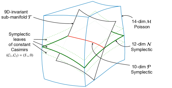
Figure 3: Different phase space sub-manifold are necessary to lift the degeneracies associated to the existence of Casimir invariants and correctly implementing the TD SSC.

IV.1.2 Symplectic structure on $\mathcal{P}$

As explained previously, we can consider only two constraints out of the four (39) to describe $\mathcal{P}$. We denote them by $C^{\mathcal{A}}$ and $C^{\mathcal{B}}$, where $\mathcal{A}$ and $\mathcal{B}$ are two fixed numbers in $(0,\ldots,3)$ (as opposed to abstract indices $(A,B,C,D,\ldots)$ which can be summed over and take any value in $(0,\ldots,3)$). Coordinates on $\mathcal{P}$ can be chosen by taking any subset of 10 from the 12 canonical coordinates on $\mathcal{N}$ (just as we did when going from to $\mathcal{M}$ to $\mathcal{N}$).

The Hamiltonian system we consider is now $(\mathcal{P},\Lambda_{\mathcal{P}},H_{\mathcal{P}})$, where $\text{dim}(\mathcal{P})=10$ and, as before, the Hamiltonian $H_{\mathcal{P}}$ is obtained by writing $H$ (in Eq. (35))) in terms of the 10 coordinates on $\mathcal{P}$ (with the help of the two constraints $C^{A}=0,C^{B}=0$ to remove the 2 discarded ones, if necessary). According to the classical theory of constrained Hamiltonian systems Deriglazov (2022), the Poisson structure $\Lambda_{\mathcal{P}}$ on $\mathcal{P}$ (inherited from that on $\mathcal{N}$, is well-defined provided that the $\mathcal{N}$-brackets $\{C^{\mathcal{A}},H\}$ and $\{C^{\mathcal{B}},H\}$ both vanish on $\mathcal{P}$, i.e., that $\mathcal{P}$ is invariant by the flow of $H$ on $\mathcal{N}$. As follows from Eq. (38), this is the case for us.

However, having a well-defined $\Lambda_{\mathcal{P}}$ does not mean that it is symplectic (non-degenerate). Again, relying on constrained Hamiltonian system theory Deriglazov (2022), $\Lambda_{\mathcal{P}}$ will be non-degenerate if and only if $\{C^{A},C^{B}\}\neq 0$ on $\mathcal{P}$. Using the Poisson brackets (11) and the relations (17), we find

$$\{C^{\mathcal{A}},C^{\mathcal{B}}\}=\eta^{CD}\pi_{C}\pi_{D}S^{\mathcal{A}\mathcal{B}}-2\pi^{[\mathcal{A}}C^{\mathcal{B}]}\,,$$ (41)

Evaluated on $\mathcal{P}$, the scalar (41) is numerically to $-\mu^{2}S^{AB}$ up to quadratic-in-spin terms, with $\mu$ the mass of the particle, and $S^{\mathcal{A}\mathcal{B}}$ is one particular tetrad component of the spin tensor, which is in general non-zero, at least not everywhere on $\mathcal{P}$. Consequently, $\Lambda_{\mathcal{P}}$ is symplectic (non-degenerate). However, the induced Poisson brackets $\{,\}^{\mathcal{P}}$ on $\mathcal{P}$ will be different to those on $\mathcal{N}$ (denoted $\{,\}$ until now). In essence, the $\mathcal{N}$-brackets must be corrected to ensure that the constraints are automatically satisfied for any calculation on $\mathcal{P}$. Thankfully, it is possible to express the $\mathcal{P}$-brackets in terms of those on $\mathcal{N}$ and the constraints. The relation is given by Arnold et al. (2006); Brown (2022)

$$\{F,G\}^{\mathcal{P}}:=\{F,G\}-\{F,C^{\mathcal{A}}\}(M^{-1})_{\mathcal{A}\mathcal{B}}\{C^{\mathcal{B}},G\}\,,$$ (42)

with $M^{-1}$ denoting the matrix inverse of the two-by-two matrix $M^{\mathcal{A}\mathcal{B}}=\{C^{\mathcal{A}},C^{\mathcal{B}}\}$. On the right-hand side of Eq. (42), the $\mathcal{N}$-Poisson brackets must be used first (for example using the 12 canonical coordinates on $\mathcal{N}$), and then the overall result is simplified using the constraints and expressed it in terms of the 10 chosen variables on $\mathcal{P}$. Notice that, by construction, for any function $F:\mathcal{P}\rightarrow\mathbb{R}$, one has $\{F,C^{\mathcal{A}}\}^{\mathcal{P}}=0$ and $\{F,C^{\mathcal{B}}\}^{\mathcal{P}}=0$, i.e., the two constraints are Casimirs of the symplectic structure $\Lambda_{\mathcal{P}}$. In our case, Eq. (42) can be simplified even more, as we have $M^{\mathcal{A}\mathcal{B}}=\{C^{\mathcal{A}},C^{\mathcal{B}}\}\mathbb{I}_{2}$, where $\mathbb{I}_{2}$ is the two-by-two canonical symplectic matrix. Therefore, from (41), we obtain

$$\{F,G\}^{\mathcal{P}}=\{F,G\}+\frac{\{F,C^{\mathcal{A}}\}\{G,C^{\mathcal{B}}\}-\{F,C^{\mathcal{B}}\}\{G,C^{\mathcal{A}}\}}{\mu^{2}S^{\mathcal{A}\mathcal{B}}}\,,$$ (43)

where $\mu^{2}$ is a function of the coordinates on $\mathcal{P}$ (equal to $-2H_{\mathcal{P}}$), just like $C^{\mathcal{A}},C^{\mathcal{B}}$ and $S^{\mathcal{A}\mathcal{B}}$.

IV.2 Summary of the formulation on $\mathcal{P}$

We can now summarize our final Hamiltonian formulation of the linearized MPTD + TD SSC equations, in the most general way (i.e., for any background metric). A thorough application of this formalism can be found in a joined paper Ramond and Isoyama (2024) for the case of the Schwarzschild metric.

• Endow $\mathcal{P}=\mathbb{R}^{10}$ with 10 coordinates chosen from the 12 canonical ones $(x^{\alpha},\sigma,\zeta,\pi_{\alpha},\pi_{\sigma},\pi_{\zeta})$ on $\mathcal{N}$. These coordinates all have a natural physical interpretation in spacetime.

• Build the Hamiltonian $H_{\mathcal{P}}$ from expressing Eq. (35) in terms of the 10 coordinates on $\mathcal{P}$. This result in a covariant expression (arbitrary spacetime coordinates and tetrad field).

• Choose two constraints $C^{\mathcal{A}},C^{\mathcal{B}}$ directly from TD SSC in (39), and compute the Poisson brackets $\{,\}^{\mathcal{P}}$ of any two phase space functions.

Doing this will result in a well-defined, covariant and non-degenerate Hamiltonian system, on a 10D phase space $\mathcal{P}$. Any physical solution to the MPTD + TD SSC system (9) will correspond to a trajectory in $\mathcal{P}$, where the TD SSC is automatically enforced at each point. These solutions are described by the law of motion (Hamilton’s equation)

$$\frac{\mathrm{d}F}{\mathrm{d}\bar{\tau}}=\{F,H_{\mathcal{P}}\}^{\mathcal{P}}\,,$$ (44)

where $F:\mathcal{P}\rightarrow\mathbb{R}$ is any phase space function, $H_{\mathcal{P}}$ is the autonomous Hamiltonian and $\bar{\tau}$ corresponds, physically, to the proper time per unit of the particle’s mass. The formulation is covariant and automatically implies the constancy of the spin norm $S_{\circ}$ (as a Casimir invariant on $\mathcal{P}$) and of the particle’s mass $\mu$, as the conserved value of the Hamiltonian along any trajectory ($\mu^{2}=-2H_{\mathcal{P}}$).

Lastly, it is worth noting that, from Eqs. (38) and (43), we have $\{F,H_{\mathcal{P}}\}^{\mathcal{P}}=\{F,H_{\mathcal{P}}\}$ for any function $F:\mathcal{P}\rightarrow\mathbb{R}$, i.e., the equations of motion on $\mathcal{P}$ can be computed thanks to Hamilton’s canonical equation on $\mathcal{N}$ and simplifying the result with the constraints. However, this is only because $\mathcal{P}$ is an invariant sub-manifold of the flow of the quantity $H_{\mathcal{P}}$ itself. In general, i.e., for any other function $G:\mathcal{P}\rightarrow\mathbb{R}$, one will have $\{F,G\}^{\mathcal{P}}\neq\{F,G\}$.

IV.3 Invariants of the MPTD system

With the final Hamiltonian formulation presented, there is only so much we can discuss if we want to remain general, i.e., independent of the metric background. Yet, it is still possible to adapt existing results in the literature regarding invariants of motion for the MPTD system itself. Since our Hamiltonian generates the same equations, we can expect these invariant to have something to do with integrals of motion for our system.

IV.3.1 Killing vectors and invariants

In the context of general relativity, most spacetime metrics of interest possesses Killing vectors, i.e., a vector field $\xi^{a}$ that satisfies Killing’s equation $\nabla_{(a}\xi_{b)}=0$. It is well-known for the MPTD equations (2) that, if $\xi^{a}$ is such a Killing vector, then the quantity

$$\Xi:=p_{\alpha}\xi^{\alpha}+\frac{1}{2}S^{\alpha\beta}\nabla_{\alpha}\xi_{\beta}\,,$$ (45)

remains constant along the worldline of the particle. In the Hamiltonian formulation, this result translates naturally. Let $\xi^{\alpha}$ be the natural components a Killing field $\xi^{a}$. In our setup, $\xi^{\alpha}$ are four functions of the phase space coordinates $x^{\alpha}$. Then combining the Hamiltonian (12) and the Poisson brackets (11) on $\mathcal{M}$ lead to

$$\{\Xi,H\}=p^{\alpha}p^{\beta}\nabla_{\alpha}\xi_{\beta}+\frac{1}{2}(\nabla_{\alpha}\nabla_{\beta}\xi_{\gamma}-R_{\gamma\beta\alpha\delta}\xi^{\delta})p^{\alpha}S^{\beta\gamma}=0\,.$$ (46)

where the first and second terms in the right-hand side vanishes independently because of Killing’s equation and the Kostant formula, respectively. Now, these Killing invariants have an additional interesting property. Let us set $C^{\alpha}:=p_{\beta}S^{\beta\alpha}$, so that the TD SSC amounts to the vanishing of the vector $C^{\alpha}$. Then, for any vector field $\xi^{\alpha}$,

$$\{C^{\alpha},\Xi\}=2S^{\alpha\beta}\nabla_{(\beta}\xi_{\gamma)}p^{\gamma}+C^{\beta}\partial_{\beta}\xi^{\alpha}\,.$$ (47)

The first term on the right-hand side of (47) vanishes by Killing’s equation, and the second one vanishes on $\mathcal{P}$, where $C^{\beta}=0$. Therefore, Killing invariants $\Xi$ commute with the constraints induced by the TD SSC. Inserting Eqs. (46) and (47) into the definition of the brackets (43) on $\mathcal{P}$, we find that for any Killing vector field $\xi^{\alpha}$ of the background spacetime,

$$\{\Xi,H\}^{\mathcal{P}}=0\,,$$ (48)

i.e., $\Xi$ is also an invariant for the constrained system on $\mathcal{P}$. In addition, we readily see from that if two Killing invariants are in involution in the full phase space, they remain so with respect to the symplectic form on $\mathcal{P}$. We stress that these results hold for Killing invariants (or any scalar function built solely from them), and not, for additional invariants that may not be associated to Killing vector fields.

IV.3.2 Killing tensors and invariants

In addition to vector fields, Killing tensors of higher valence may exist and lead to invariants of motion Frolov et al. (2017). Of particular interest are the (symmetric) Killing-Stäckel tensors $K_{ab}$, such that $\nabla_{(a}K_{bc)}=0$, and the (antisymmetric) Killing-Yano tensors $Y_{ab}$ such that $\nabla_{(a}Y_{b)c}$=0. For our purposes, we take inspiration from the pioneering work of Rüdiger on Killing invariants for the MPTD system Rüdiger (1981, 1983) (see also the more recent and complete work on the matter in Compère and Druart (2022)). In these works, the authors look for scalar quantities built from $p_{a},S^{ab}$ and the geometry that are conserved under the dipolar MPTD system under the TD SSC. As a result, they find that in spacetimes with a Killing-Yano tensor $Y_{ab}$, two such invariants exist. The first one is

$$\mathfrak{K}:=\frac{1}{4}\varepsilon_{abcd}Y^{ab}S^{cd}\,.$$ (49)

In contrast to Killing vector invariants (45) which are exactly conserved for the general dipolar MPTD system (without any SSC), the Rüdiger invariant $\mathfrak{K}$ is referred to as a “quasi-invariant”, since its derivative along $\mathscr{L}$ is not zero, but of quadratic order in spin: $\nabla_{u}\mathfrak{K}=O(\epsilon^{2})$, in the sense of (8). The other Rüdiger invariant, which we denote by $\mathfrak{Q}$, is

$$\mathfrak{Q}:=K^{ab}p_{a}p_{b}+4\varepsilon_{ade[b}Y^{e}_{~{}c]}\mathfrak{y}^{a}S^{db}p^{c}\,,$$ (50)

where $K^{ab}$ is the Killing-Stäckel tensor Carter (2009) associated to $Y_{ab}$ and $\mathfrak{y}^{a}$ is the Hodge dual of $\nabla_{a}Y_{bc}$, both uniquely defined from $Y_{ab}$ through $K^{ab}:=Y^{a}_{~{}c}Y^{bc}$ and $\nabla_{a}Y_{bc}:=\varepsilon_{abcd}\mathfrak{y}^{d}$. Again, $\mathfrak{Q}$ is only conserved at linear order in spin.

Interestingly, in the non-spinning (geodesic) case $S^{ab}=0$, one has $\mathfrak{K}=0$ and $\mathfrak{Q}=K^{ab}p_{a}p_{b}$, which only requires the existence of a Killing-Stäckel tensor $K_{ab}$, not a Killing-Yano tensor Dietz and Rüdiger (1981); Dietz and Rudiger (1982). In the Kerr spacetime, $K^{ab}p_{a}p_{b}$ is the well-known Carter constant Carter (1968) that ensures the integrability of geodesics.

IV.3.3 Covariant notion of angular momentum

Lastly, let us mention that the two Rüdiger invariants $\mathfrak{K},\mathfrak{Q}$ can be given a physical interpretation related to a covariant notion of angular momentum tied to the Killing-Yano tensor. This was discussed in Frolov et al. (2017); Witzany (2019); Compère and Druart (2022), but first pointed out by Dietz and Rüdiger in Dietz and Rüdiger (1981); Dietz and Rudiger (1982). Let us define the following quantities

$$\quad S^{b}_{\text{\tiny{TD}}}:=\frac{1}{2}\varepsilon^{abcd}\bar{p}_{a}S_{cd}\quad\text{and}\quad L^{b}:=p_{a}Y^{ab}\,,$$ (51)

where $S^{a}_{\text{\tiny{TD}}}$ is the spin 4-vector measured by an observer of four-velocity $\bar{p}_{a}$ (recall the general decomposition in IV.1). Then $L^{a}$ can be interpreted as a covariant notion of angular momentum in the sense that, in the Schwarzschild spacetime, its spatial components admit the correct Newtonian limit $\vec{L}=\vec{r}\times\vec{p}$ at spatial infinity, like in a spherically symmetric Newtonian potential. This analogy is explored in our follow-up paper within Schwarzschild Ramond and Isoyama (2024), where explicit formulae are given.

Combining the definitions (51) with the decomposition (5) (with $f^{a}=\bar{p}^{a}$), we can re-write the two Rüdiger invariants (49),(50) as

$$\mathfrak{K} =-\frac{1}{\mu}L_{a}S^{a}_{\text{\tiny{TD}}}+O(C^{a})\,,$$ (52a)

$$\mathfrak{Q} =L^{a}L_{a}-2\mu Y_{ab}S_{\text{\tiny{TD}}}^{a}\mathfrak{y}^{b}+\mathfrak{K}\,p_{a}\mathfrak{y}^{a}+O(C^{a})\,,$$ (52b)

where the fact that $L^{a}$ and $S^{a}_{\text{\tiny{TD}}}$ are orthogonal to $p_{a}$ was used, and $O(C^{a})$ describes a term proportional to $C^{b}:=p_{a}S^{ab}$, which vanishes under the TD SSC (6). From Eq. (52), we thus can interpret the first invariant $\mathfrak{K}$ as the projection of the spin 4- vector onto the angular momentum 4-vector $L^{a}$, and the second invariant $\mathfrak{Q}$ as the (spin-corrected) squared norm of the $L^{a}$. Interestingly Compère and Druart (2022), in the Kerr spacetime one has $\mathfrak{y}^{a}=(\partial_{t})^{a}$ so the third term in (52b) is actually independently conserved from $\mathfrak{Q}$, as the product $\mathfrak{K}\cdot(-E)$, where $E:=-\pi_{t}$ is the conserved total energy of the particle, as discussed in Sec. V.3 below.

V Application: integrability around black holes

In this section, we apply our Hamiltonian formulation to the case of a Schwarzschild and Kerr background. In both cases, the resulting system is found to be integrable, in the usual sense of Liouville, i.e, as defined in the classical reference Arnold et al. (2006) (or Hinderer and Flanagan (2008) for the general relativistic case including non-compact dimensions). Even though the integrability in Kerr evidently implies that in Schwarzschild as a particular case, the latter admits a number of unique features worth discussing first (in Sec. V.2) before moving on to the general, Kerr case (in Sec. V.3).

V.1 Preliminaries

The matter of integrability of the motion of spinning particles in black hole spacetimes has been studied in the past, but its current status is still, mostly, in a state of conjecture, and based on numerical studies. To be as clear as possible, we start by recalling the classical definition of integrable Hamiltonian systems, following classical references, like Arnold et al. (2006), but see also Hinderer and Flanagan (2008) and references therein for subtleties in the relativistic case.

Let $(\mathcal{P},\{,\}^{\mathcal{P}},H_{\mathcal{P}})$ be a Hamiltonian system, where $\text{dim}(\mathcal{P})=2N\in\mathbb{N}$ and where $\{,\}^{\mathcal{P}}$ is a non-degenerate Poisson bracket on $\mathcal{P}$. A first integral of the system $(\mathcal{P},\{,\}^{\mathcal{P}},H_{\mathcal{P}})$ is a function $\mathcal{I}:\mathcal{P}\rightarrow\mathbb{R}$ such that $\{\mathcal{I},H_{\mathcal{P}}\}^{\mathcal{P}}=0$. Two first integrals $(\mathcal{I}_{1},\mathcal{I}_{2})$ are in involution if they satisfy $\{\mathcal{I}_{1},\mathcal{I}_{2}\}^{\mathcal{P}}=0$. A set of $n\in\mathbb{N}$ first integrals $(\mathcal{I}_{1},\ldots,\mathcal{I}_{n})$ is said to be linearly independent if the matrix constructed from their gradients has maximal rank (equal to $n$) on $\mathcal{P}$. The system $(\mathcal{P},\{,\}^{\mathcal{P}},H_{\mathcal{P}})$ is integrable if it admits (i) $N=\text{dim}(\mathcal{P})/2$ first integrals that are (ii) linearly independent and (iii) in pairwise involution. It is crucial that all three items above be verified. In particular, we stress that a Casimir invariant can be used as a first integral, as its mere existence violates the requirement of non-degeneracy of $\{,\}^{\mathcal{P}}$. Similarly, the particle mass $\mu^{2}=$, as the on-shell value of our autonomous Hamiltonian, is readily promoted to a first integral. Lastly, we emphasize that everything that follows (like the rest of the article) is done consistently at linear order in spin, i.e., in the small parameter $\epsilon=S_{\circ}/\mu M$, with $M$ the black hole mass (cf. the discussion in Sec. I.4).

With all necessary precautions now taken, we can now apply the above result with $N=5$ to our Hamiltonian formalism, summarized in Sec. IV.2, in the Schwarzschild and Kerr spacetimes.

V.2 Integrability in the Schwarzschild spacetime

V.2.1 Geometry and Hamiltonian

In this subsection, we let $(\mathscr{E},g_{ab})$ be the Schwarzschild spacetime. To specify the canonical variables on $\mathcal{N}$, by making a choice of coordinates covering $\mathscr{E}$ and a choice of orthonormal tetrad. We choose the Schwarzschild-Droste (SD) coordinates $x^{\alpha}=(t,r,\theta,\phi)$, in which the contravariant components $g^{\alpha\beta}$ of the metric read Gourgoulhon (2021)

$$g^{tt}=-\frac{1}{f(r)}\,,\quad g^{rr}=f(r)\,,\quad g^{\theta\theta}=\frac{1}{r^{2}}\,,\quad g^{\phi\phi}=\frac{\csc^{2}\theta}{r^{2}}\,,$$ (53)

where $f(r)=1-2M/r$, $M$ being the Schwarzschild mass parameter. Because the metric is diagonal, an orthonormal tetrad can be obtained by normalizing the natural basis $(\partial_{\alpha})^{a}$ associated to the coordinates $x^{\alpha}$. We find, in terms of this basis, the tetrad

$$(e_{0})^{a}=\frac{1}{\sqrt{f}}(\partial_{t})^{a}\,,\quad(e_{1})^{a}=\sqrt{f}(\partial_{r})^{a}\,,\quad(e_{2})^{a}=\frac{1}{r}(\partial_{\theta})^{a}\,,\quad(e_{3})^{a}=\frac{\csc\theta}{r}(\partial_{\phi})^{a}\,.$$ (54)

For the Hamiltonian (35) we also need the connection 1-forms $\omega_{aBC}=(e_{B})_{b}\nabla_{a}(e_{C})^{b}$, and, more specifically, their components in the natural basis, $\omega_{\alpha BC}$, which are explicitly needed for the transformation (16). A direct calculation shows that, out of the 24 Ricci coefficients, only eight are non vanishing, and found to be (see also Müller and Grave (2009) but with different conventions):

$$\omega_{t01}=-\frac{M}{r^{2}}\,,\quad\omega_{\theta 12}=-\sqrt{f}\,,\quad\omega_{\phi 31}=\sqrt{f}\sin\theta\,,\quad\omega_{\phi 23}=-\cos\theta\,,$$ (55)

and the four other obtained by the algebraic antisymmetry $\omega_{\alpha BC}=-\omega_{\alpha CB}$. Inserting formulae (53) and (54) into the generic Hamiltonian (35), we obtain

$$H_{\mathcal{N}}=-\frac{\pi_{t}^{2}}{2f}+\frac{f\pi_{r}^{2}}{2}+\frac{1}{2r^{2}}\left(\pi_{\theta}^{2}+\frac{\pi_{\phi}^{2}}{\sin^{2}\theta}\right)-\frac{\pi_{\phi}\cos\theta}{r^{2}\sin^{2}\theta}S^{1}+\frac{\pi_{\phi}\sqrt{f}}{r^{2}\sin\theta}S^{2}-\frac{\sqrt{f}\pi_{\theta}}{r^{2}}S^{3}+\frac{M\pi_{t}}{r^{2}f}D^{1}\,,$$ (56)

where it is understood that one replaces the spin components $\vec{S},\vec{D}$ using Eqs. (29). By construction, the Hamiltonian (56) generates the linear-in-spin dynamics of a spinning particle in a Schwarzschild spacetime. It depends on 3 parameters $M,S_{\circ},S_{\star}$ and 12 phase space variables arranged as symplectic pairs: the six degrees of freedom $(t,r,\theta,\phi,\sigma,\zeta)$ and their conjugated momenta $(\pi_{t},\pi_{r},\pi_{\theta},\pi_{\phi},\pi_{\sigma},\pi_{\zeta})$. Lastly, the two constraints coming from the TD SSC (37), as prescribed in Sec. IV.2, are chosen to be setting $\mathcal{A}=0$ and $\mathcal{B}=1$. In terms of the phase space coordinates, they read, respectively,

$$C^{0} =-\sqrt{f}\pi_{r}D^{1}-\frac{\pi_{\theta}}{r}D^{2}-\frac{\pi_{\phi}}{r\sin\theta}D^{3}=0\,,$$ (57a)

$$C^{1} =\frac{\pi_{t}}{\sqrt{f}}D^{1}+\frac{\pi_{\phi}}{r\sin\theta}S^{2}-\frac{\pi_{\theta}}{r}S^{3}=0\,,$$ (57b)

where, again, $\vec{S},\vec{D}$ are functions of $(\sigma,\pi_{\sigma},\zeta,\pi_{\zeta})$ via Eqs. (29).

V.2.2 First integrals

The symmetries of the Schwarzschild spacetime are in correspondence with four Killing vectors. Given in the natural basis $(\partial_{\alpha})^{a}$ associated to the SD coordinates $x^{\alpha}=(t,r,\theta,\phi)$, they read

$$\xi_{(t)}^{a} =(\partial_{t})^{a}\,,$$ (58a)

$$\xi_{(x)}^{a} =-\sin\phi(\partial_{\theta})^{a}-\cos\phi\cot\theta\,(\partial_{\phi})^{a}\,,$$ (58b)

$$\xi_{(y)}^{a} =\cos\phi(\partial_{\theta})^{a}-\sin\phi\cot\theta\,(\partial_{\phi})^{a}\,,$$ (58c)

$$\xi_{(z)}^{a} =(\partial_{\phi})^{a}\,.$$ (58d)

The four Killing vectors (58) imply the existence of four Killing invariants of the form (45). In terms of the canonical coordinates on $\mathcal{N}$, these read

$$E :=-\pi_{t}\,,$$ (59a)

$$J_{x} :=-\sin\phi\,\pi_{\theta}-\cos\phi\cot\theta\,\pi_{\phi}+\cos\phi\csc\theta\,S^{1}\,,$$ (59b)

$$J_{y} :=\cos\phi\,\pi_{\theta}-\sin\phi\cot\theta\,\pi_{\phi}+\sin\phi\csc\theta\,S^{1}\,,$$ (59c)

$$J_{z} :=\pi_{\phi}\,,$$ (59d)

where the first invariant, associated to the Killing vector $-\xi_{(t)}^{a}$, is denoted $E$ according to its interpretation as the total energy of the particle as measured by an observer at rest at infinity Gourgoulhon (2021), and the last three are denoted according to their classical interpretation as three Cartesian components of a conserved angular-momentum 3-vector $\vec{J}$. This vector is orthogonal to an invariant Euclidean plane to which the motion of the particle stays close, but in which it is not confined. We emphasize that, in spite of their notation, these invariants include both orbital and spin contributions hidden in the $\pi_{\alpha},\pi_{\sigma}$ variables (cf. Eq. (16)).

V.2.3 Invariants from the Killing-Yano tensor

The Schwarzschild spacetime admits a Killing-Yano tensor Tanaka et al. (1996); Açık et al. (2010); Compère and Druart (2022), whose components in the natural basis are given by

$$Y^{ab}=\frac{2}{r\sin\theta}(\partial_{\theta})^{[a}(\partial_{\phi})^{b]}\,,$$ (60)

and it is manifestly antisymmetric. Squaring the Killing-Yano tensor generates a Killing-Stäckel tensor $K^{ab}$ though the combination $K^{ab}:=Y^{ac}Y^{b}_{\phantom{c}c}$. Using (60), we find

$$K^{ab}=(\partial_{\theta})^{a}(\partial_{\theta})^{b}+\frac{1}{\sin^{2}\!\theta}\,(\partial_{\phi})^{a}(\partial_{\phi})^{b}\,.$$ (61)

When we substitute Eqs. (16), (60) and (61) within Eqs. (49) and (50), we obtain the explicit expressions for the Rüdiger quasi-invariants $\mathfrak{K}$ and $\mathfrak{Q}$ in terms of the canonical coordinate on $\mathcal{N}$:

$$\mathfrak{K} =rD^{1}\,,$$ (62a)

$$\mathfrak{Q} =\pi_{\theta}^{2}+\frac{\pi_{\phi}^{2}}{\sin^{2}\theta}-\frac{2\pi_{\phi}\cos\theta}{\sin^{2}\theta}S^{1}\,,$$ (62b)

where $D^{1}$ is a function of $(\sigma,\pi_{\sigma},\zeta,\pi_{\zeta})$ via Eq. (29).

V.2.4 Integrability

To prove the integrability, we need to (i) exhibit five first integrals, which are (ii) linearly independent on $\mathcal{P}$ and (iii) in pairwise involution.

The first item is easy to verify. There are seven first integral “candidates” obtain from Killing symmetries: four in Eqs. (59), two in Eqs. (62) and the Hamiltonian (56). The fact that they are (indeed) first integrals for $H_{\mathcal{P}}$ is also easy to check, as follows. First, $H_{\mathcal{P}}$ is trivially so as an autonomous Hamiltonian. Second, all four $(E,J_{x},J_{y},J_{z})$ are first integrals by the general result (48) for Killing vectors. Third, a direct calculation reveals that

$$\{\mathfrak{K},H_{\mathcal{N}}\}=-\sqrt{f}\,{C}^{0}\,,\quad\text{and}\quad\{\mathfrak{Q},H_{\mathcal{N}}\}=0\,.$$ (63)

This equation reveals that the invariant $\mathfrak{K}$ is not a first integral on $\mathcal{N}$ (i.e., when the TD SSC is not applied), as should be expected Rüdiger (1981, 1983); Compère and Druart (2022). However, inserting Eqs. (63) into the $\mathcal{P}$-brackets (43) and applying the constraints to the right-hand side gives $\{\mathfrak{K},H_{\mathcal{P}}\}^{\mathcal{P}}=0$ and $\{\mathfrak{Q},H_{\mathcal{P}}\}^{\mathcal{P}}=0$. Now, to their linear independence. It is already compromised from the fact that

$$\mathfrak{Q}={J_{x}}^{2}+{J_{y}}^{2}+{J_{z}}^{2}$$ (64)

as follows from Eqs. (59) and (62b). This is, again, somewhat expected from the spherical symmetry of the Schwarzschild spacetime, as discussed in Ramond and Isoyama (2024). Removing, say, $J_{x}$ from the list leaves us with 6 first integrals $(H_{\mathcal{P}},E,J_{y},J_{z},\mathfrak{K},\mathfrak{Q})$, which are easily checked to be linearly independent. Lastly, their involution. This is compromised too, since, as is well-known, the angular-momentum components verify $\{J_{y},J_{z}\}=J_{x}$, again this is associated to the spherical symmetry (see, e.g., Zelenka et al. (2020)). We can thus drop one of them, say $J_{y}$. However, all five first integrals in the final set $(H_{\mathcal{P}},E,J_{z},\mathfrak{K},\mathfrak{Q})$ are in involution, since the only non-trivial brackets to verify is $\{\mathfrak{K},\mathfrak{Q}\}^{\mathcal{P}}$. However, from combining Eqs. (57) and (62), we easily show the following identities

$$\{\mathfrak{K},\mathfrak{Q}\}=0\,,\quad\{\mathfrak{K},C^{0}\}=\frac{\pi_{t}\mathfrak{K}}{\sqrt{f}}\,,\quad\{\mathfrak{K},C^{1}\}=-\sqrt{f}\pi_{r}\mathfrak{K}\,,\quad\{\mathfrak{Q},C^{0}\}=0\,,\quad\{\mathfrak{Q},C^{1}\}=0\,.$$ (65)

Inserting all these identities into Eq. (43) readily leads to $\{\mathfrak{K},\mathfrak{Q}\}^{\mathcal{P}}=0$. This confirms that $(H_{\mathcal{P}},E,J_{z},\mathfrak{K},\mathfrak{Q})$ are in involution on $\mathcal{P}$, thereby concluding the proof of integrability.

It is clear that the spherical symmetry of the Schwarzschild spacetime plays a leading role into the integrability of the system. However, this symmetry is also the reason why, out of the seven initial first integrals, two were discarded. In addition, the Killing vectors are not enough: while $\mathfrak{Q}$ actually comes from the spherical invariance (because it equals $\vec{J}\cdot\vec{J}$), $\mathfrak{K}$ exists only thanks to the Killing-Yano tensor, and is independent of the Killing vectors. Therefore, it seems that the Killing-Yano structure, even on the Schwarzschild spacetime, is key to the integrability.

V.3 Integrability in the Kerr spacetime

Most remarkably, all five first integrals $(H_{\mathcal{P}},E,J_{z},\mathfrak{K},\mathfrak{Q})$ that ensure integrability in Schwarzschild have an equivalent in the Kerr spacetime, thus suggesting that integrability can be naturally extended to the latter. We will show that this is precisely the case, following the exact same steps. We use the following shorthands in this section (and only in this section): $\Sigma:=r^{2}+a^{2}\cos\theta$, $\Delta:=r^{2}-2Mr+a^{2}$, $\delta^{2}=a^{2}+r^{2}$, $c=\cos^{2}\theta$ and $s=\sin\theta$.

V.3.1 Geometry and Hamiltonian

In terms of the Boyer-Lindquist (BL) coordinates $x^{\alpha}=(t,r,\theta,\phi)$, the contravariant components of the Kerr metric read Gourgoulhon (2021)

$$g^{tt}=-\frac{2a^{2}Mrs^{2}+\delta^{2}\Sigma}{\Sigma\Delta}\,,\,g^{\theta\theta}=\frac{1}{\Sigma}\,,\,g^{rr}=\frac{\Delta}{\Sigma}\,,\,g^{\phi\phi}=\frac{\Sigma-2Mr}{\Sigma\Delta s^{2}}\,,\,g^{\phi t}=g^{t\phi}=-\frac{2aMr}{\Delta\Sigma}\,,$$ (66)

where $M\geq 0$ is interpreted as black hole’s mass and the spin parameter $a\in[0;M]$ is such the angular momentum of the black hole is $aM$. For $a=0$, one recovers the Schwarzschild metric (53). To construct the canonical coordinates for the spin on $\mathcal{N}$, we shall use the Carter tetrad Gourgoulhon (2021). In terms of the natural basis $(\partial_{\alpha})^{a})$ associated to the BL coordinates, the Carter tetrad is defined by

$$(e_{0})^{a}:=\frac{\delta^{2}\,(\partial_{t})^{a}+a\,(\partial_{\phi})^{a}}{\sqrt{\Delta\Sigma}}\,,\,(e_{1})^{a}:=\sqrt{\frac{\Delta}{\Sigma}}\,(\partial_{r})^{a}\,,\,(e_{2})^{a}:=\frac{(\partial_{\theta})^{a}}{\sqrt{\Sigma}}\,,\,(e_{3})^{a}:=\frac{as\,(\partial_{t})^{a}+(\partial_{\phi})^{a}/s}{\sqrt{\Sigma}}\,.$$ (67)

The non-vanishing components of the connection 1-forms $\omega_{aBC}$ associated to the Carter tetrad are easily computed and read:

$$\omega_{t01} =\frac{M}{\Sigma^{2}}(a^{2}c^{2}-r^{2})\,,\,\,\omega_{t23}=\frac{2acMr}{\Sigma^{2}}\,,\,\,\omega_{r03}=\frac{ars}{\sqrt{\Delta}\,\Sigma}\,,\,\,\omega_{r12}=-\frac{a^{2}cs}{\sqrt{\Delta}\,\Sigma}\,,$$ (68a)

$$\omega_{\theta 03} =-\frac{ac\sqrt{\Delta}}{\Sigma}\,,\,\,\omega_{\theta 12}=-\frac{\sqrt{\Delta}r}{\Sigma}\,,\,\,\omega_{\phi 01}=\frac{as^{2}}{\Sigma^{2}}\left(a^{2}c^{2}(r-M)+r^{2}(M+r)\right)\,,$$ (68b)

$$\omega_{\phi 02} =\frac{ac\sqrt{\Delta}s}{\Sigma}\,,\,\omega_{\varphi 13}=-\frac{\sqrt{\Delta}rs}{\Sigma}\,,\,\omega_{\phi 23}=\frac{c}{\Sigma^{2}}(a^{2}\Delta s^{2}-\delta^{2})\,.$$ (68c)

Again, setting $a=0$ in the coefficients leads to their Schwarzschild expressions (55). The Hamiltonian on $\mathcal{N}$, which we re-write from (12) using Eqs. (18), reads

$$H_{\mathcal{N}}=\frac{1}{2}g^{\alpha\beta}\pi_{\alpha}\pi_{\beta}+\frac{1}{2}g^{\alpha\beta}\pi_{\alpha}\left(\omega_{\beta IJ}\varepsilon^{IJ}_{\phantom{IJ}K}S^{K}+2\omega_{\beta 0I}D^{I}\right)\,,$$ (69)

in which all formulae (66) and (68) can be inserted to get an explicit expression. Similarly, all the above ingredients can be used to compute the two constraints $(C^{0},C^{1})=(0,0)$ given by Eq. (39), which read

$$\sqrt{\Sigma}\,C^{0} :=-\sqrt{\Delta}\pi_{r}D^{1}-(a\pi_{t}\sin\theta+\pi_{\phi}\csc\theta)D^{3}-\pi_{\theta}D^{2}\,,$$ (70a)

$$\sqrt{\Delta\Sigma}\,C^{1} :=(a\pi_{\phi}+\delta^{2}\pi_{t})\,D^{1}+\sqrt{\Delta}\left((a\pi_{t}\sin\theta+\pi_{\varphi}\csc\theta)\,S^{2}-\pi_{\theta}S^{3}\right)\,.$$ (70b)

V.3.2 First integrals

The Kerr spacetime is stationary just like the Schwarzschild one, but spherical symmetry is lost and replaced by asymmetry. Consequently, only two Killing vectors of (58) remain, namely:

$$\xi_{(t)}^{a}=(\partial_{t})^{a}\quad\text{and}\quad\xi_{(z)}^{a}=(\partial_{\phi})^{a}\,.$$ (71)

These Killing vectors lead to the existence of two Killing invariants from Eq. (45), expressed in terms of the coordinates on $\mathcal{N}$ as

$$E:=-\pi_{t}\quad\text{and}\quad L_{z}:=\pi_{\phi}\,,$$ (72)

and have the same physical interpretation as in the Schwarzschild case (total energy, and angular-momentum along the symmetry axis, measured at infinity). They are automatically promoted as first integrals thanks to the general result (48). In the Kerr spacetime, there alse exists a Killing-Yano tensor, which admits a simple expression in terms of the Carter tetrad (67), namely Floyd (1973); Compère and Druart (2022)

$$Y^{ab}:=2r(e_{2})^{[a}(e_{3})^{b]}-2a\cos\theta(e_{0})^{[a}(e_{1})^{b]}\,,$$ (73)

Once again, this Killing-Yano tensor generates the Killing-Stäckel $K^{ab}:=Y^{ac}Y^{b}_{\phantom{b}c}$, whose expression is readily obtained as

$$K^{ab}=r^{2}\,\bigl{(}(e_{2})^{a}(e_{2})^{b}+(e_{3})^{a}(e_{3})^{b}\bigr{)}+a^{2}\cos^{2}\!\theta\,\bigl{(}(e_{0})^{a}(e_{0})^{b}-(e_{1})^{a}(e_{1})^{b}\bigr{)}\,.$$ (74)

Inserting Eqs. (73) and (74) within the definition of the two Rüdiger invariants (49) and (50) leads to their expression in terms of the canonical coordinates on $\mathcal{N}$

$$\mathfrak{K} =r\,D^{1}+a\cos\theta\,S^{1}\,,$$ (75a)

$$\mathfrak{Q} =\mathfrak{Q}_{0}+\vec{\mathfrak{Q}}_{S}\cdot\vec{S}+\vec{\mathfrak{Q}}_{D}\cdot\vec{D}\,,$$ (75b)

where $\mathfrak{Q}_{0},\vec{\mathfrak{Q}}_{S},\vec{\mathfrak{Q}}_{S}$ are spin-independent quantities given by

$$\Sigma\,\Delta\,\mathfrak{Q}_{0} :=\pi_{\phi}^{2}(a^{4}c^{2}s^{2}+\Delta r^{2})/s^{2}+2a^{2}c^{2}M\pi_{t}^{2}r^{3}+\Delta(\pi_{\theta}^{2}r^{2}-a^{2}c^{2}\Delta\,\pi_{r}^{2})$$ (76a)

$$\,\,\,+a\pi_{t}(a\pi_{t}+2\pi_{\phi})(a^{2}c^{2}\delta^{2}+\Delta\,r^{2})\,,$$ (76b)

$$\Sigma\,\mathfrak{Q}_{S}^{1} :=2(a\pi_{\phi}+\delta^{2}\pi_{t})\,ac-2r^{2}\pi_{\phi}c/s^{2}\,,$$ (76c)

$$\sqrt{\Delta}\,\Sigma^{2}\,\mathfrak{Q}_{S}^{2} :=4ar\left(ac^{2}((2Mr-a^{2})\pi_{\phi}\csc{\theta}+a\Delta s\pi_{t})-r^{2}(s\pi_{t}\delta^{2}+2a\pi_{\phi}\csc{\theta})\right)\,,$$ (76d)

$$\Sigma^{2}\,\mathfrak{Q}_{S}^{3} :=2a^{2}\sqrt{\Delta}\left(\pi_{\theta}c-r\pi_{r}s\right)rc\,,$$ (76e)

$$\Delta\,\Sigma\,\mathfrak{Q}_{D}^{1} :=2a^{2}c^{2}\left((a^{2}-3r^{2})M\pi_{t}+a\pi_{\phi}(M-r)\right)-2ar\left(\Delta(\pi_{\phi}+a\pi_{t})-c^{2}\delta^{2}a\pi_{t}\right)\,,$$ (76f)

$$\sqrt{\Delta}\,\Sigma^{2}\,\mathfrak{Q}_{D}^{2} :=-2a^{2}\left(a^{2}c^{3}\Delta s\pi_{t}+a(c^{2}(a^{2}-2Mr)+r^{2})\pi_{\phi}\cot\theta+c\delta^{2}r^{2}s\pi_{t}\right)\,,$$ (76g)

$$\Sigma^{2}\,\mathfrak{Q}_{D}^{3} :=2a\sqrt{\Delta}(a^{2}c^{3}\pi_{\theta}+r^{3}\pi_{r}s)\,.$$ (76h)

Unlike in the Schwarzschild case, we have at our disposal five first integral “candidates”, namely $(H_{\mathcal{P}},E,L_{z},\mathfrak{K},\mathfrak{Q})$. This is just enough to ensure integrability, as shown below.

V.3.3 Integrability

We do exactly the same checks as we did in Schwarzschild to ensure that all five invariants defined are (i) first integrals for $H_{\mathcal{P}}$ and (ii) linearly independent. The calculations become quickly complicated by hand, and can be found in the companion Mathematica Notebook MMA (2024). The last ingredient to check is the pairwise involution of all these first integrals. Again, this present no difficulty and only the bracket $\{\mathfrak{K},\mathfrak{Q}\}^{\mathcal{P}}$ is non-trivial. The latter is zero, ensuring that $(H_{\mathcal{P}},E,L_{z},\mathfrak{K},\mathfrak{Q})$ satisfy all properties for the 10D Hamiltonian system $(\mathcal{P},\{,\}^{\mathcal{P}},H_{\mathcal{P}})$ to be integrable in Kerr, thus concluding the proof.

Before we end this section, we want to emphasize on an interesting feature that unexpectedly stumbled upon. Quite remarkably, we found a much stronger result than $\{\mathfrak{K},\mathfrak{Q}\}^{\mathcal{P}}=0$, namely

$$\{\mathfrak{Q},H\}=0\,,\quad\text{and}\quad\{C^{A},\mathfrak{Q}\}=\alpha^{A}_{\phantom{A}B}C^{B}\,,$$ (77)

for some coefficients $\alpha^{A}_{\phantom{A}B}$ that only depend on $(\pi_{t},r,\pi_{r},\theta,\pi_{\theta},\pi_{\phi})$. The result (77) readily implies $\{\mathfrak{K},\mathfrak{Q}\}^{\mathcal{P}}=0$ (owing to Eq. (43)), but also that $\mathfrak{Q}$, as given in (50), is actually a first integral of the 12D system on $\mathcal{N}$, just like a Killing vector invariant would be. This is a very special result: it does not hold for $\mathfrak{K}$, and it is unclear if it holds for other Ricci-flat spacetimes.

Conclusions and prospects

Concluding summary

This article contains two main results. The first one is a rigorous and covariant Hamiltonian framework for the linear-in-spin dynamics in any given metric, under the TD SSC. The framework is summarized in Sec. IV.2. The final formulation on the 10D phase space $\mathcal{P}$ is the only one that is well-posed theoretically, in the sense that the SSC is automatically enforced along any trajectory, and practically, because the structure is symplectic and one can use the classical tool from Hamiltonian mechanics. The reduction to $\mathcal{P}$ went in two steps. First, we went from a 14D, degenerate formulation on the phase space $(x^{\alpha},p_{\alpha},S^{\alpha\beta})\in\mathcal{M}$, to a 12D, symplectic (non-degenerate) formulation on $(x^{\alpha},\pi_{\alpha},\sigma,\pi_{\sigma},\zeta,\pi_{\zeta})\in\mathcal{N}$ (the symplectic leaves of $\mathcal{M}$). In particular, these coordinates on $\mathcal{N}$ are canonical, and we provided a simple physical interpretation for them. Lastly, we enforced the Tulczyjew-Dixon spin supplementary condition, treating it a phase space constraint, thereby restricting to a 10D, symplectic (non-degenerate) formulation on $\mathcal{P}$. All physical solutions to the algebraic-differental system (9)-(6) fill the 10D phase space $\mathcal{P}$.

The general covariance of the framework, its 10-dimensional nature and the rigorous treatment of different kinds of “constants” of motion, are the key aspects of the formulation, compared to other existing Hamiltonian constructions available in the literature, in particular Barausse et al. (2009) and Witzany et al. (2019). These features are made possible by the use of the Tulczyjew-Dixon spin supplementary condition (SSC). As we argued in Sec. I.3, this SSC plays a special role in our framework, and it is possible that it is the only SSC for which such rigorous, covariant and 10D treatment is possible in the first place.

The second main result is the application of our formalism to the case of the Schwarzschild and Kerr spacetimes. By exhibiting enough independent integrals of motion in Sec. V, we have shown that the system is integrable, at linear order in spin. This result disproves the conjecture that exists chaotic motion for the linear-in-spin MPTD + TD SSC system. The five functionally independent integrals of motion admit a very simple interpretation, summarized in Table. 1. They were all known already in 1981, following Rüdiger’s work on the MPTD + TD SSC invariants. These invariants simply lacked a well-defined Hamiltonian framework in which to be interpreted as first integrals. Our work clearly identifies the role of the Killing-Yano tensor (or hidden symmetry) of both the Kerr and Schwarzschild spacetime as the source of this integrability at linear-in-spin order. In particular, Kerr is once again very special, since all the first integrals $E,L_{z},\mathfrak{K},\mathfrak{Q}$ can be related to existence of the sole Killing-Yano tensor of the Kerr spacetime, as the latter uniquely seeds the two Killing vectors Hughston and Sommers (1973), a property unique to Kerr.

Symmetry	First integral	Killing structure
free particle	$\mu:$ mass	Metric $g_{ab}$
stationarity	$E:$ total energy	Killing vector $(\partial_{t})^{a}$
axisymmetry	$L_{z}:$ $z$-comp. of ang. mom.	Killing vector $(\partial_{\phi})^{a}$
hidden symmetry	$(\mathfrak{K},\mathfrak{Q}):$ Rüdiger’s spin invariants	Killing-Yano tensor $Y_{ab}$

Table 1: Symmetries at play behind integrability of spinning particles around Kerr black holes.

Future applications

This article is the first in a series aiming at exploiting the powerful machinery of Hamiltonian mechanics to study the MPTD equations. Now that the general framework is established and that integrability for black hole backgrounds is proven, our next step is to perform practical implementations and solve specific problems. We now make a (non-exhaustive) list of potential prospects, some of which are already ongoing.

Canonical formulation and solutions by quadrature

The final, 10-dimensional formulation on the phase space $\mathcal{P}$ (summarized in Sec. IV.2) is not endowed with canonical coordinates. We do not think this is possible to do in the general case, i.e., without first making a choice for the background metric. However, once such choice is made, nothing prevents us from constructing such coordinates from the non-canonical ones. A method for doing just this is, in fact, is already present in this paper, in App. B, where we construct the map $S^{AB}\in\mathbb{R}^{6}\mapsto(\sigma,\pi_{\sigma},\zeta,\pi_{\zeta})$ by explicitly solving the $S^{AB}$-brackets by viewing them as canonical brackets between $(\sigma,\pi_{\sigma},\zeta,\pi_{\zeta})$-dependent functions. This is an example of non-canonical to canonical coordinate transformation.

In a follow-up article Ramond and Isoyama (2024), we have managed to do this reduction in a Schwarzschild background, i.e., we have explicitly constructed 10 canonical coordinates on $\mathcal{P}$, thus giving a canonical formulation of the linear-in-spin dynamics. These coordinates turn the 5D Hamiltonian into an effective 1D one for the radial motion, with the 8 other phase space coordinates taking the form of (cyclic angle,first integral) pairs; with the first integrals being precisely $(E,J_{z},\mathfrak{Q},\mathfrak{K})$. This formulation permits an analytic solution in terms of elliptic functions. Generalization to the Kerr case is ongoing.

Action-angle variables, frequencies and resonances

Since the linear-in-spin dynamics in the Kerr spacetime form an integrable system, the Liouville-Arnold theorem Liouville (1855); Arnold et al. (2006) ensures that there exists a particular set of canonical variables $(\mathcal{J}_{i},\vartheta_{i})_{\{i=1,\ldots,5\}}$, called action-angle variables. The actions $\mathcal{J}_{i}$ are in a 1-to-1 correspondence with the five integrals of motion $(\mu,E,L_{z},\mathfrak{K},\mathfrak{Q})$. To our knowledge, these have never been derived for generic Schwarzschild or Kerr orbits in linear-in-spin motion. These variables are probably the best (if not the only) tool to study resonances in the system linear-in-system, with the well-defined, gauge-invariant notion of Hamiltonian frequencies $\Omega_{i}:=\partial H_{\mathcal{P}}/\partial\mathcal{J}_{i}$. These frequencies are presented for the Schwarzschild case in the follow-up article Ramond and Isoyama (2024). They will allow us to study the impact of linear-in-spin terms on orbital resonances, as well as spin-orbit resonances. In essence, this will extend the geodesic analyses of Brink et al. (2015) for conservative resonances, and Flanagan and Hinderer (2012) for transient resonances (when dissipation is turned on).

First law of mechanics and flux-balance laws

By adapting the methods of Le Tiec (2014), it should be possible to derive a first law of mechanics for a two-body system made of a dipolar particle orbiting a Kerr black hole, at linear order in spin. The first law, at this order, has been derived in the past, in different contexts (e.g.g, using the ADM Hamiltonian formalism Blanchet et al. (2013), or for circular orbits using the helical symmetry in Ramond and Le Tiec (2022)). This new derivation would give some insight as to the status of these laws, extend their domain of validity, but most of all, it would allow for a very convenient way to extract the conservative part of the second-order gravitational self-force, as linear-in-spin effects enter precisely at this order Mathews et al. (2022).

In the context of adiabatic evolution for asymmetric binaries Pound and Wardell (2021), it is possible to derive so-called “flux-balance laws” for the constants of motion that are slowly evolving under the emission of gravitational waves. These laws encode crucial information about the dissipative sector of the gravitational self-force. When these constants of motion are associated to spacetime isometries (like $E$ or $L_{z}$ in Kerr), the derivation of such laws is well-understood for geodesics Isoyama et al. (2019). When linear-in-spin effects are included, the study Akcay et al. (2020) extended these results for energy and angular-momentum. Recently, the authors of Grant and Moxon (2023b) proposed a method based on symplectic currents to construct these laws for constants of motion that are not associated to spacetime isometries, for example the Carter constant in the non-spinning case. This method could be generalized for the Rüdiger constants $\mathfrak{K},\mathfrak{Q}$ that fit in this category.

Adding the self-force to the linear-in-spin formalism

It has been shown that for a non-spinning particle orbiting a Kerr black hole, the conservative part of the self-force does not break the integrability of the system Vines and Flanagan (2015b); Fujita et al. (2017). It is still unclear if this holds true at linear order in spin, or whether couplings between the self-force effects and spin breaks integrability. Nevertheless, it is now well-established that the conservative self-force can be absorbed into a re-definition of the background metric to an effective one Shah et al. (2011); Barack (2014); Pound and Wardell (2021); Harte (2015), such that there is hope to write a (possibly) covariant Hamiltonian framework that does just this (see also Blanco and Flanagan (2023a, b) on this matter). Ref Isoyama et al. (2019) was able to do this for a Kerr background and non-spinning case, and we hope to extend this analysis to the linear-in-spin case.

Regarding the dissipative sector of the self-force, one must leave the realm of classical conservative Hamiltonian systems. Indeed, the prime effect of dissipation is to make the constants of motion evolve adiabatically. However, there is hope that Galley’s Hamiltonian formulation of non-conservative mechanics Galley (2013) may apply to this context. It was already successfully applied in the context of effective field theory Galley and Leibovich (2012), and we plan to explore its application in ours in the future.

Hairy black holes, electromagnetic fields

The extension of our integrability result to other spacetimes (in particular other black hole metrics) should be straightforward, even though integrability will most probably only follow if there are enough Killing symmetries. It would be interesting to investigate integrability for axisymmetric, stationary spacetimes admitting Killing-Yano tensors, relying on classification to explore all possibilities. In addition, if one accounts for electromagnetic fields, for example in the case of charged black holes, then an additional linear-in-spin coupling appears in the Hamiltonian (cf. the generalized momentum-velocity relation in Gralla et al. (2010) or the added terms in the Poisson structure d’Ambrosi et al. (2016)). One cannot say if this additional term will break integrability or not, because of what becomes of the Killing tensors under these additional fields. We leave all these extensions for future investigations.

Quadratic-in-spin dynamics

In this article, all calculations are done consistently at linear order in the spin $S^{ab}$, cf. Sec. I.4. This linearization is not so much a simplifying constraint than it is a necessary assumption for the dipolar MPTD equations to be physically self-consistent. A natural extension to our work is, therefore, to include quadratic-in-spin effects in our Hamiltonian. While this is easily done at dipolar order by adapting the construction of Witzany et al. (2019), self-consistency requires that we go to quadrupolar order, where a spin-induced quadrupole arises on the left-hand-side of Eq. (2), see Harte (2020); Compère et al. (2023). We have managed to extend our covariant Hamiltonian formulation to this quadratic-in-spin order, which will be the object a forthcoming publication Ramond et al. (2024). To our knowledge, there exists no quadratic-in-spin and covariant Hamiltonian formulation of these quadratic-in-spin equations, the closest to this being the self-consistent (but non-covariant) quadratic-in-spin Hamiltonian of Vines et al. (2016). One interesting aspect of having a quadratic-in-spin Hamiltonian is that it is a perturbation of the linear-in-spin one, presented here. Therefore, it should be possible to analytically study the emergence of chaos there, using the Melnikov-Poincaré theory Wiggins (2013); Guckenheimer and Holmes (2013), and the impact it can have on the motion, especially around resonances, as described by Kolmogorov-Arnold-Moser theory, and around fixed points, as described by Poincaré-Birkhoff theory Arnold et al. (2006). We aim to explore this effect in the future.

We note that the non-integrability of quadratic-in-spin dynamics, in both Schwarzschild and Kerr, have currently no analytical proofs but only numerical evidence. If the secondary is a neutron star, the system is probably non-integrable, because of the arbitrarily complex matter fields at play. However, when the secondary is a black hole, both Rüdiger constants $\mathfrak{K},\mathfrak{Q}$ that we have used in this work admit a generalization to quadratic-in-spin order Compère et al. (2023). Whether these invariants are real first integrals of the corresponding (quadratic-in-spin) Hamiltonian system and whether they are functionally independent to ensure integrability will be the subject of subsequent work.

Appendix A Conventions and notations

Throughout the paper, we use geometric units in which $G=c=1$, and our conventions for the Riemann curvature tensor and other geometric tensors are as in Wald (1984), in particular $\nabla_{a}\nabla_{b}\omega_{c}=R_{abc}^{\phantom{abc}d}\omega_{d}$ for any 1-form $\omega_{a}$. We use $a,b,c,d,\ldots$ to denote abstract indices. For the components, we use two kinds of indices varying in $\{0,1,2,3\}$ : $\alpha,\beta,\gamma,\delta,\ldots$ are used for components in the natural basis $(\partial_{\alpha})^{a}$ associated to a spacetime coordinate system $x^{\alpha}$, and $A,B,C,D,\ldots$ are used for components in an orthonormal tetrad basis $(e_{A})^{a}$. Calligraphic indices $\mathcal{A},\mathcal{B},\mathcal{C},\ldots$ are used to denote a fixed index (never summed over). An arrow is sometimes used to denote Euclidean 3-vectors, using interchangeably $\vec{v}=(v^{1},v^{2},v^{3})=v^{I}$, as well as usual notations $\cdot$ for the scalar product and $\times$ for the cross product. In the phase space, pairs of canonical coordinates are always of the form $(q,\pi_{q})$, with $\pi_{q}$ being the conjugated momentum of some degree of freedom $q$. Poisson brackets are denoted with the brackets $\{\cdot,\cdot\}$. A table for the frequently used symbols, description and references is given in Table. 2.

Table 2: List of frequently used symbols.

Notation	Description	Relevant reference
Spacetime
$\mathscr{E}$	Lorentzian manifold
$x^{\alpha}$	spacetime coordinates
$(\partial_{\alpha})^{a}$	natural vector basis
$g_{ab}$	metric tensor on $\mathscr{E}$
$R_{abcd}$	Riemann curvature tensor
$\nabla_{a}$	covariant derivative
$\varepsilon_{abcd}$	Levi-Civita tensor
$\xi^{a}$	Killing vector	(58), (71)
$Y^{ab}$	Killing-Yano tensor	(60), (73)
$K^{ab}$	Killing-Stäckel tensor	(61), (74)
$(e_{A})^{a}$	orthonormal tetrad	(54), (67)
$\omega_{aBC}$	connection 1-forms	(55), (68)
Particle
$\mathscr{L}$	particle’s worldline
$p_{a}$	momentum 1-form
$S^{ab}$	antisymmetric spin tensor
$\mu,S_{\circ},S_{\star}$	dynamical mass, spin norms	(3)
$\tau,u^{a}$	proper time, four-velocity	(7)
$S^{a}_{\text{TD}},C^{a}$	spin and mass dipole wrt $p^{a}$	(5)   $[f^{a}=\bar{p}^{a}]$
$S^{a},D^{a}$	spin and mass dipole wrt $(e_{0})^{a}$	(5)   $[f^{a}=(e_{0})^{a}]$
$\Xi$	Killing vector invariant	(59), (72)
$\mathfrak{K}$	First Rüdiger invariant	(62a), (75a)
$\mathfrak{Q}$	Second Rüdiger invariant	(62b), (75b)
Phase space
$\mathcal{M}$	14D phase-space	II.1.1
$\mathcal{N}$	12D symplectic leaves	II.4.3
$\mathcal{T}$	9D sub-manifold (TD SSC)	IV.1
$\mathcal{P}$	10D physical phase space	(40)
$\mathcal{C}_{\circ},\mathcal{C}_{\star}$	Casimir invariants	(24)
$H,H_{\mathcal{P}}$	Hamiltonian on $\mathcal{N}$, on $\mathcal{P}$	(12), (35)
$\Lambda,\{\,,\}$	Poisson structure, brackets on $\mathcal{M}$ or $\mathcal{N}$	(11), (19)
$\Lambda_{\mathcal{P}},\{\,,\}^{\mathcal{P}}$	Poisson structure, brackets on $\mathcal{P}$	(43)
$\mathcal{C}^{\mathcal{A}},\mathcal{C}^{\mathcal{B}}$	Constraints from TD SSC	(37)

Appendix B Construction of canonical coordinates for $(S^{I},D^{I})$

We now turn to the derivation of the formulae (29). This is a technical section, but with ideas that can be transposed to other constructions of symplectic variables from non-symplectic ones. Motivated by the discussion in Sec. III, we shall refer to $\vec{S}=(S^{1},S^{2},S^{3})$ as the spin variables, and to $\vec{D}=(D^{1},D^{2},D^{3})$ as the dipole variables. We shall perform the derivation in four successive steps detailed below. The strategy is to use brute force and to solve for the system of nine coupled partial differential equations (PDE) obtained by writing explicitly the Poisson brackets (19) for $(\vec{S},\vec{D})$ in terms of $(\sigma,{\pi_{\sigma}},\zeta,{\pi_{\zeta}})$, i.e., using the formula

$$\{F,G\}=\frac{\partial F}{\partial\sigma}\frac{\partial G}{\partial{\pi_{\sigma}}}-\frac{\partial G}{\partial\sigma}\frac{\partial F}{\partial{\pi_{\sigma}}}+\frac{\partial F}{\partial\zeta}\frac{\partial G}{\partial{\pi_{\zeta}}}-\frac{\partial G}{\partial\zeta}\frac{\partial F}{\partial{\pi_{\zeta}}}\,,$$ (78)

which holds for any functions $F,G$ of the (looked-for) symplectic variables $(\sigma,{\pi_{\sigma}},\zeta,{\pi_{\zeta}})$.

B.1 Spin sector $S^{I}$

Our starting point is the assumption that we can parameterize the vector $\vec{S}$ using only one (say $\sigma$) out of the two angles $(\sigma,\zeta)$ available. The motivation is simple: in the limit where the dipole vanishes $\vec{D}=0$, the variables should resemble the usual symplectic variables of SO(3). Under our assumption, in the vanishing dipole limit, the coordinate conjugated to $\zeta$ will be absent, and its conjugate ${\pi_{\zeta}}$ a constant of motion (thanks to Hamilton’s equations). This invariant should correspond to the Casimir invariant of the SO(3) algebra, namely the norm of $\vec{S}$. Guided by this SO(3) analogy, our initial Ansatz for $\vec{S}$ reads

$$S^{1}=F_{1}(\sigma,{\pi_{\sigma}},{\pi_{\zeta}})\,,\quad S^{2}=F_{2}(\sigma,{\pi_{\sigma}},{\pi_{\zeta}})\quad\text{and}\quad S^{3}=F_{3}(\sigma,{\pi_{\sigma}},{\pi_{\zeta}})\,,$$ (79)

where the functions $F_{1},F_{2},F_{3}$ are to be determined. Next, we make a symplectic transformation that makes $F_{3}(\sigma,{\pi_{\sigma}},{\pi_{\zeta}})$ the new variable conjugated to $\sigma$. The other variables are then changed accordingly, but since they are unconstrained at this point, we may as well rename them and consider, without loss of generality, that our Ansatz is

$$S^{1}=F({\pi_{\sigma}},{\pi_{\zeta}},\sigma)\,,\quad S^{2}=G({\pi_{\sigma}},{\pi_{\zeta}},\sigma)\quad\text{and}\quad S^{3}={\pi_{\sigma}}\,,$$ (80)

where the functions $F,G$ are to be determined. With the form (80), the Poisson brackets (19b), written in terms of the symplectic coordinates as in (78), take the simple form

$$\frac{\partial F}{\partial\sigma}\frac{\partial G}{\partial{\pi_{\sigma}}}-\frac{\partial G}{\partial\sigma}\frac{\partial F}{\partial{\pi_{\sigma}}}={\pi_{\sigma}}\,,\quad\frac{\partial G}{\partial\sigma}=F\quad\text{and}\quad-\frac{\partial F}{\partial\sigma}=G\,.$$ (81)

The last two brackets readily imply that $S^{1}=f_{1}\cos\sigma+f_{2}\sin\sigma$ and $S^{2}=-f_{2}\cos\sigma+f_{1}\sin\sigma$, for some functions $f_{1}({\pi_{\sigma}},{\pi_{\zeta}})$ and $f_{2}({\pi_{\sigma}},{\pi_{\zeta}})$ to be determined. Inserting the latter in the first equation of (81) and solving leads to $f_{1}^{2}+f_{2}^{2}=f({\pi_{\zeta}})^{2}-\pi_{\sigma}^{2}$ for some arbitrary positive function denoted $f({\pi_{\zeta}})^{2}$. Without loss of generality, one can take $f=\text{id}$ and $f_{2}=0$, the former thanks to the simple symplectic change of coordinates $(\zeta,{\pi_{\zeta}})\mapsto(\zeta/f^{\prime}({\pi_{\zeta}}),f({\pi_{\zeta}}))$, and the latter because of the inherent SO(3) invariance of the brackets (19b) for $\vec{S}$. In the end, this leads to our final formulae for $\vec{S}$, namely

$$S^{1}=\sqrt{\pi_{\zeta}^{2}-\pi_{\sigma}^{2}}\cos\sigma\,,\quad S^{2}=\sqrt{\pi_{\zeta}^{2}-\pi_{\sigma}^{2}}\sin\sigma\quad\text{and}\quad S^{3}={\pi_{\sigma}}\,,$$ (82)

as given in our main result Eqs. (29).

Having now fully exploited the three brackets (19b) satisfied by $\vec{S}$ to simplify the calculations, we now turn to finding coordinates for the dipole $\vec{D}$ with the formulae (82) at hand.

B.2 Dipole sector $D^{I}$

B.2.1 Preliminaries

The fact that $S^{3}(\sigma,{\pi_{\sigma}},\zeta,{\pi_{\zeta}})={\pi_{\sigma}}$ leads to remarkably simple brackets in the dipole sector. Starting with the three brackets $\{D^{I},S^{3}\}$ with $I=1,2,3$ from (19d), we find

$$\frac{\partial D^{3}}{\partial\sigma}=0\,,\quad\frac{\partial D^{1}}{\partial\sigma}=-D^{2}\quad\text{and}\quad\frac{\partial D^{2}}{\partial\sigma}=D^{1}\,.$$ (83)

The first equation simply means that $D^{3}=D^{3}({\pi_{\sigma}},\zeta,{\pi_{\zeta}})$, and the last two readily imply that $D^{1},D^{2}$ are of the form

$$D^{1}=A\cos\sigma+B\sin\sigma\quad\text{and}\quad D^{2}=A\sin\sigma-B\cos\sigma\,,$$ (84)

where $A,B$ are functions of $({\pi_{\sigma}},\zeta,{\pi_{\zeta}})$ to be determined. The Poisson bracket $\{D^{2},S^{2}\}=0$ from (19d) then implies that $B$ is actually independent of ${\pi_{\sigma}}$. Therefore, so far

$$D^{1} =A({\pi_{\sigma}},\zeta,{\pi_{\zeta}})\cos\sigma+B(\zeta,{\pi_{\zeta}})\sin\sigma\,,$$ (85a)

$$D^{2} =A({\pi_{\sigma}},\zeta,{\pi_{\zeta}})\sin\sigma-B(\zeta,{\pi_{\zeta}})\cos\sigma\,,$$ (85b)

$$D^{3} =D^{3}({\pi_{\sigma}},\zeta,{\pi_{\zeta}})\,.$$ (85c)

B.2.2 Finding $A$ and $B$

From the brackets $\{S^{1},D^{2}\}$ and $\{D^{1},S^{2}\}$ in Eq. (19d) we obtain after some lengthy but straightforward algebra two PDEs for $A$ and $B$, namely

$${\pi_{\sigma}}B={\pi_{\zeta}}\frac{\partial A}{\partial\zeta}\quad\text{and}\quad{\pi_{\zeta}}\frac{\partial B}{\partial\zeta}+{\pi_{\sigma}}A=(\pi_{\sigma}^{2}-\pi_{\zeta}^{2})\frac{\partial A}{\partial{\pi_{\sigma}}}\,,$$ (86)

where we used $\partial B/\partial{\pi_{\sigma}}=0$ along the way. Differentiating the second equation with respect to $\zeta$ and using the first one to eliminate $A$ with the help of Schwartz’ theorem to swap the second derivatives, we obtain the simple equation $\partial^{2}B/\partial\zeta^{2}+B=0$, resulting in

$$B(\zeta,{\pi_{\zeta}})=b_{1}({\pi_{\zeta}})\cos\zeta+b_{2}({\pi_{\zeta}})\sin\zeta\,,$$ (87)

for some functions $b_{1}$ and $b_{2}$. Inserting this result back into the first equation of (86) and integrating with respect to $\zeta$ then leads to the following expression for $A$,

$$A({\pi_{\sigma}},\zeta,{\pi_{\zeta}})=\frac{{\pi_{\sigma}}}{{\pi_{\zeta}}}\bigl{(}b_{1}({\pi_{\zeta}})\sin\zeta-b_{2}({\pi_{\zeta}})\cos\zeta\bigr{)}+a({\pi_{\zeta}},{\pi_{\sigma}})\,,$$ (88)

for some function $a({\pi_{\zeta}},{\pi_{\sigma}})$. The latter can be found by inserting both Eqs. (87) and (88) into the second equation of (86). One obtains a PDE for $a({\pi_{\sigma}},{\pi_{\zeta}})$ that integrates into

$$a({\pi_{\sigma}},{\pi_{\zeta}})=a_{0}({\pi_{\zeta}})\sqrt{\pi_{\zeta}^{2}-\pi_{\sigma}^{2}}\,,$$ (89)

for some unknown function $a_{0}({\pi_{\zeta}})$. Lastly, from the expressions (87)–(89) for $A$, $B$ and $a$ we obtain that of $D^{3}$ by using either of the two brackets $\{S^{1},D^{2}\}=D^{3}$ and $\{D^{1},S^{2}\}=D^{3}$. They lead to the same result, namely

$$D^{3}({\pi_{\sigma}},\zeta,{\pi_{\zeta}})=\sqrt{1-\frac{\pi_{\sigma}^{2}}{\pi_{\zeta}^{2}}}\left(b_{2}({\pi_{\zeta}})\cos\zeta-b_{1}({\pi_{\zeta}})\sin\zeta\right)+a_{0}({\pi_{\zeta}}){\pi_{\sigma}}\sqrt{\pi_{\zeta}^{2}-\pi_{\sigma}^{2}}\,.$$ (90)

It turns out that the remaining brackets from (19d) are of no additional help because of the Jacobi identity, which gives a relation between all Poisson brackets, making them not all independent from one another. Hence, we turn to the brackets (19c) to finish the calculation.

B.2.3 Integration “constants”

At this point the expressions for $\vec{D}$ depend on three unknown functions of the variable ${\pi_{\zeta}}$ alone, namely $a_{0}$, $b_{1}$ and $b_{2}$. To find them we start from either of the two brackets $\{D^{2},D^{3}\}=-S^{1}$ or $\{D^{3},D^{1}\}=-S^{2}$ from Eq. (19c). They lead to the same PDE, of the form

$$\left(A\frac{\partial D^{3}}{\partial{\pi_{\sigma}}}+\{D^{3},B\}_{(\zeta,{\pi_{\zeta}})}-\sqrt{\pi_{\zeta}^{2}-\pi_{\sigma}^{2}}\right)\cos\sigma+\left(B\frac{\partial D^{3}}{\partial{\pi_{\sigma}}}-\{D^{3},A\}_{(\zeta,{\pi_{\zeta}})}\right)\sin\sigma=0\,,$$ (91)

where $\{\cdot\}_{(\zeta,\pi_{\zeta})}$ is the bracket with respect to the sole pair $(\zeta,\pi_{\zeta})$. Since both terms in parentheses are independent of $\sigma$, we obtain, thanks to the linear independence of $\sigma\mapsto\cos\sigma$ and $\sigma\mapsto\sin\sigma$, two independent PDEs. Now we can substitute for the current expressions of $A,B,D^{3}$ given in Eqs. (88), (87) and (90) into each, and after many simplifications, the first one turns into an elementary ODE for the unknown $a_{0}({\pi_{\zeta}})$:

$$\frac{\mathrm{d}a_{0}}{\mathrm{d}{\pi_{\zeta}}}+\frac{2a_{0}}{{\pi_{\zeta}}}=0\quad\Rightarrow\quad a_{0}({\pi_{\zeta}})=\frac{C_{1}}{\pi_{\zeta}^{2}}\,,$$ (92)

for some constant $C_{1}\in\mathbb{R}$; while the second PDE implies an algebraic relation between $b_{1}$ and $b_{2}$:

$$b_{1}\frac{\mathrm{d}b_{1}}{\mathrm{d}{\pi_{\zeta}}}+b_{2}\frac{\mathrm{d}b_{2}}{\mathrm{d}{\pi_{\zeta}}}={\pi_{\zeta}}+\frac{C_{1}^{2}}{{\pi_{\zeta}}^{3}}\quad\Rightarrow\quad b_{1}({\pi_{\zeta}})^{2}+b_{2}({\pi_{\zeta}})^{2}=\pi_{\zeta}^{2}-\frac{C_{1}^{2}}{\pi_{\zeta}^{2}}-C_{2}\,,$$ (93)

for some constant $C_{2}\in\mathbb{R}$. At this point, the only remaining unknown function is either $b_{1}$ or $b_{2}$. It can be checked that all remaining Poisson brackets are consistent with any choice of $b_{1},b_{2}$ provided that the constraint (93) is verified. This is the same degeneracy that occurs in the SO(3) case, as already mentioned in Sec. B.1 for the Ansatz for $\vec{S}$. In order to obtain the simplest end result, we set $b_{2}({\pi_{\zeta}})=0$, such that our last remaining unknown function is found to be (we chose the positive square root with no loss of generality)

$$b_{1}({\pi_{\zeta}})=\sqrt{\pi_{\zeta}^{2}-\frac{C_{1}^{2}}{\pi_{\zeta}^{2}}-C_{2}}\,,$$ (94)

and the two constants $C_{1},C_{2}$ remain arbitrary.

At this point our results are (82) for $\vec{S}$, and a combination of (94), (92) and (85) through (90) for $\vec{D}$. We can use these expressions to compute the two Casimir invariants $S_{\circ},S_{\star}$ given by (24). Most conveniently, we obtain the very simple result

$$C_{1}=S_{\star}^{2}\quad\text{and}\quad C_{2}=S_{\circ}^{2}\,.$$ (95)

This concludes the proof of the expressions of $(\vec{S},\vec{D})$ in terms of the symplectic coordinates $(\sigma,{\pi_{\sigma}},\zeta,{\pi_{\zeta}})$ and the invariants $(S_{\circ},S_{\star})$, as provided in our main result (29).

Appendix C Identities for the coordinates $(x^{\alpha},\pi_{\alpha},S^{I},D^{I})$

C.1 Derivation of Poisson brackets

C.2 Jacobi identity

Showing that the Poisson brackets (11) satisfy the Jacobi identity is straightforward but lengthy. However, the calculation can be shortened as follows. First, we use the coordinates $(y^{1},\ldots,y^{1}4)=(x^{\alpha},\pi_{\alpha},S^{I},D^{I})$, which are in a 1-to-1 correspondence with $(x^{\alpha},\pi_{\alpha},S^{\alpha\beta})$, and, second, the equivalence between the Jacobi identity. Whether the Jacobi identity holds is, indeed, invariant under isomorphisms. Second, we can use the Jacobi identity in the equivalent form $\sum_{\text{cycle}}\{y^{i},\{y^{j},y^{k}\}\}=0$, cf. Deriglazov (2022). Since any bracket involving one $x^{\alpha}$ or one $\pi_{\alpha}$ is either 0 or 1, the Jacobi identity will be verified for any triplet that includes at least one instance of $x^{\alpha}$ or $\pi_{\alpha}$. For the other triplets, only four combinations are possible, thanks to the anti-symmetry of Poisson brackets. For example,

$$\{S^{I}\!,\{S^{J}\!,S^{K}\}\}+\{S^{K}\!,\{S^{I}\!,S^{J}\}\}+\{S^{J}\!,\{S^{K}\!,S^{I}\}\}=(\varepsilon^{IJL}\varepsilon^{KLM}\!+\varepsilon^{JKL}\varepsilon^{ILM}\!+\varepsilon^{KIL}\varepsilon^{JLM})S^{M}\,,$$

where we used the brackets $\eqref{PBsSD}$ and the fact that $\varepsilon^{IJK}\in\{-1,0,1\}$. Using the identity $\varepsilon^{IJK}\varepsilon^{LMK}=\delta^{IL}\delta^{JM}-\delta^{IM}\delta^{JL}$, the right-hand side of this equation is readily seen to vanish. All three other possibilities (schematically $\{S,\{S,D\}\}$, $\{S,\{D,D\}\}$ and $\{D,\{D,D\}\}$), follow exactly the same pattern and vanish for the same reason.

Appendix D Hamiltonian systems and generalizations

In this Appendix, we provide a summary of several non-equivalent notions related to Hamiltonian systems. To be clear, by Hamiltonian system, we mean a general framework in which a scalar function $H$ defined on some phase space manifold $\mathcal{M}$ gives rise, through some geometrical structure $\Lambda$, to a set of first order differential equations (ODES). Our aim is to be concise and self-contained, and to give an explicit definition of every notion that is, usually, defined implicitly. There exists many different formulations of Hamiltonian systems in the literature, with different levels of abstraction and generality. These differences are mainly concerned with the dimensionality of the phase space and the geometric structure thereon. We shall cover the ones necessary for our purposes. They include (i) canonical symplectic systems, (ii) non-canonical symplectic systems (iii) Poisson (non-symplectic) systems Our Hamiltonian formulation of the linearized MPTD + TD SSC system requires each of these four notions.

Even though all these notions can be given a coordinate-free exposition (with tensor algebra and differential geometry on the phase space manifold), we will instead choose to always work with coordinates since 1) in applications one will practically never use the coordinate-free application and 2) we do not want to mix things up with the covariant formulation of objects in GR. We refer to the recent introductory exposition Deriglazov (2022) which is at once detailed and pedagogical. Otherwise, classical textbooks such as Arnold et al. (2006) and Vaisman (2012) are always recomended.

D.1 Symplectic systems

The main distinction between different notions of Hamiltonian systems has to do with the geometrical structure on the phase space, which generates a vector field (trajectories) from the Hamiltonian function. This structure is a closed bilinear form, which, when non-degenerate, is called “symplectic”. Therefore, in what follows, symplectic is a place-holder for “non-degenerate”. The degenerate case will be dealt with later in Sec .D.2.

D.1.1 Canonical

Perhaps without knowing it, one is always introduced to symplectic systems during one’s first course on analytical mechanics. There, one learns that a $2n$-dimensional Hamiltonian system is a set of ordinary differential equations (ODEs) for some unknowns quantities $(q,p)=(q^{i},p_{i})_{i\in\{1,\ldots,n\}}$. There are always an even number of such unknowns (here $2n$ for some $n\in\mathbb{N}$), and the ODEs that they satisfy are called Hamilton’s equations:

$$\frac{\mathrm{d}q^{i}}{\mathrm{d}\lambda}=\frac{\partial H}{\partial p_{i}}\quad\text{and}\quad\frac{\mathrm{d}p_{i}}{\mathrm{d}\lambda}=-\frac{\partial H}{\partial q^{i}}\,,$$ (96)

where $H:\mathbb{R}^{2n}\rightarrow\mathbb{R}$ is a scalar function of the $(q,p)$ called the Hamiltonian, and $\lambda$ is the parameter associated to $H$, usually (but not necessarily) related to some kind of “time”. What makes this formulation canonical is that and the $2n$ variables $(q_{i},p_{i})$ always come in $n$ pairs, referred to as conjugated pairs. These variables span a $2n$-dimensional phase space $\mathcal{P}\subset\mathbb{R}^{2n}$, on which each point corresponds to a (possible) configuration of the underlying physical system. On top of this classical picture, one will occasionally be introduced to the notion of Poisson bracket. This is defined as an operation between two smooth functions $F:\mathcal{P}\rightarrow\mathbb{R}$ and $G:\mathcal{P}\rightarrow\mathbb{R}$, defined by

$$\{F,G\}=\sum_{j=1}^{n}\,\left(\,\frac{\partial F}{\partial q_{j}}\frac{\partial G}{\partial p^{j}}-\frac{\partial G}{\partial q_{j}}\frac{\partial F}{\partial p^{j}}\,\right)\,.$$ (97)

The Poisson bracket is useful because it can be used to re-write the evolution of any function $F:\mathcal{P}\rightarrow\mathbb{R}$ along a solution to Hamilton’s equations (96) as follows. Using the chain rule, as well as Eqs. (96) and (97), one readily finds

$$\frac{\mathrm{d}F}{\mathrm{d}\lambda}=\{F,H\}\,.$$ (98)

Therefore, the evolution of any function $F:\mathcal{P}\rightarrow\mathbb{R}$ along a phase space trajectory is given by its Poisson bracket with $H$. From the definition (97), the Poisson brackets of two coordinates, say $q^{i},p^{j}$, are also easy to find. One obtains the well-known formula

$$\{q^{i},p_{j}\}=\delta^{i}_{j}\,,$$ (99)

where $\delta^{i}_{j}$ is the Kronecker symbol. Equation (99) is called the canonical Poisson brackets, and is a characterization of canonical coordinates. In other words, Eq. (99) is equivalent to the word “canonical” in the phrase “canonical Hamiltonian system”, or to the word “conjugated” in “conjugated pairs of variables”, all these notions being tautological. There are infinitely many distinct systems of canonical coordinates, all linked to one another through canonical transformations. The reason canonical variables on $\mathcal{P}$ are so useful in Hamiltonian mechanics is because 1) the general form of Hamilton’s equation (96), 2) the definition (98) of the Poisson bracket of two arbitrary functions, and 3) the fundamental brackets between canonical coordinates (99), are all invariant under canonical transformations. In other words, if $(q,p)\in\mathbb{R}^{2n}\mapsto(Q,P)\in\mathbb{R}^{2n}$ is a canonical transformation, then one can simply substitute $(q,p)$ by $(Q,P)$ in Eqs. (96), (98) and (99), where it is understood that the Hamiltonian $H$ and the functions $F,G$ are expressed in terms of $(Q,P)$.

D.1.2 Non-canonical

In spite of their usefulness, a canonical formulation of is but a very special way of doing Hamiltonian mechanics. Sometimes, as is the case in the present article, such a formulation is not available in the first place. What happens if we use some coordinates that do not satisfy the canonical brackets (99)? This, in essence, is answered by the broader field of symplectic geometry: a more abstract generalization of Hamiltonian mechanics, of which we give a simplified overview below.

Let us start from some canonical coordinates $(q,p)\in\mathbb{R}^{2n}$ covering a phase space $\mathcal{P}$, and a non-canonical change of coordinates, i.e., a diffeomorphism $\Phi:(q,p)\in\mathbb{R}^{2n}\mapsto y\in\mathbb{R}^{2n}$. Note that, since the new coordinates $y=(y^{1},\ldots,y^{2n})$ are not canonical, there is no reason to identify them as pairs, like the $(q,p)$. Let us pick two, say $(y^{i},y^{j})$. Seing these as two functions of the $(q,p)$, we can compute their Poisson bracket using the canonical formula Eq. (97), and obtain the result in terms of $(q,p)$. According to the characterization (99) of canonical coordinates, we expect $\{y^{i},y^{j}\}\neq\delta^{ij}$ since $y$ are not canonical. Nevertheless, using the map $\Phi$, we can express any occurrence of $(q,p)$ in the resulting formula in terms of the $y$. We thus obtain the Poisson bracket $\{y^{i},y^{j}\}$ expressed solely in terms of $y$. Doing this for each pair determines a set of Poisson brackets for the $y$ coordinates, given by $4n^{2}$ formulae of the form:

$$\{y^{i},y^{j}\}=\Lambda^{ij}(y)\,,$$ (100)

where the explicit form of the right-hand side will strongly depend on the chosen coordinates. The $y$-dependent matrix $\Lambda$ whose entries are $\Lambda^{ij}(y)=\{y^{i},y^{j}\}$ is called the Poisson matrix for the coordinates $y$. Equation (100) generalizes the canonical formula (99) to non-canonical coordinates.

The Poisson matrix (100) of the coordinates $y$ on $\mathcal{P}$ is necessary and sufficient to do anything one would have done with canonical coordinates. For example, the Poisson bracket of any two functions $F(y),G(y)$ on is simply given by

$$\{F,G\}=\sum_{i,j}\,\Lambda^{ij}(y)\,\frac{\partial F}{\partial y^{i}}\,\frac{\partial G}{\partial y^{j}}\,.$$ (101)

where only the Leibniz rule and (100) was used. Equation (101) generalizes the canonical formula (97) to non-canonical coordinates $y$. Similarly, the evolution of one coordinate $y^{i}$ under some Hamiltonian $H(y)$ is obtained directly from (101) with $F=y^{i}$ and $G=H$, leading to

$$\frac{\mathrm{d}y^{i}}{\mathrm{d}\lambda}=\sum_{j}\,\Lambda^{ij}(y)\,\frac{\partial H}{\partial y^{j}}\,,$$ (102)

again, generalizing Hamilton’s canonical equations (96) to the non-canonical case. Note that Eqs. (101) and (102) can be simply written as the product of gradients of scalar functions and the matrix $\Lambda$.

The non-canonical formulation shows that, given some phase space $\mathcal{M}$ and a Hamiltonian $H$, the key quantity that encode all information about the geometry (and thus the dynamics of the system) are the Poisson brackets between some coordinates $y$ on $\mathcal{M}$ (non-necessarily canonical). Naturally, one could ask whether, given some manifold $\mathcal{M}$ endowed with some coordinates $z$ on it, a set of brackets is actually sufficient in order to define a Hamiltonian system. The answer lies in a yet more general formulation, that of Poisson systems, which, in general, are degenerate.

D.2 Non-symplectic (Poisson) systems

The Poisson system formulation of a Hamiltonian system relies on the following ingredients. Let it be given (i) a manifold $\mathcal{M}$ of dimension $N\in\mathbb{N}$ endowed with some coordinates $y=(y^{1},\ldots,y^{N})$, (ii) a scalar function $H(y)$ on $\mathcal{M}$ and (iii) a set of Poisson brackets between the $y$. In what we have presented so far, items (i) and (ii) are well-defined, but (iii) is not: the definition (101) of Poisson bracket relied on the assumption that the system was non-degenerate. In the present context, the Poisson bracket is defined as an operation between two functions $F(y),G(y)$ on $\mathcal{M}$, defined by

$$\{F,G\}=\sum_{i,j}\,\Lambda^{ij}(y)\,\frac{\partial F}{\partial y^{i}}\,\frac{\partial G}{\partial y^{j}}\,.$$ (103)

where the coefficients $\Lambda_{ij}(y)$ satisfy the following two properties:

Skew-symmetry: $$\Lambda^{ij}=-\Lambda^{ji}\,,$$ (104a)

Jacobi identity: $$\Lambda^{i\ell}\partial_{\ell}\Lambda^{jk}+\Lambda^{j\ell}\partial_{\ell}\Lambda^{ki}+\Lambda^{k\ell}\partial_{\ell}\Lambda^{ij}=0\,,$$ (104b)

where a sum from $\ell=1$ to $\ell=N$ is implied and $\partial_{\ell}=\partial/\partial y^{\ell}$. In other words, defining a Poisson system is a very general process: it is done by the choice of a $N\times N$ antisymmetric matrix whose coefficients $\Lambda^{ij}(y)$ verify the condition (104b). Again, one refers to $\Lambda(y)$ as the Poisson matrix of the system. Replacing $(F,G)$ in Eq. (104) by two coordinates $(y^{i},y^{j})$, we find the meaning of its coefficients:

$$\Lambda^{ij}(y)=\{y^{i},y^{j}\}\,.$$ (105)

What then makes a Poisson system different from a symplectic system in non-canonical coordinates? This question is natural since, after all, Eqs. (103) and (105) for Poisson systems look very much like Eqs. (101) and  (100) for non-canonical systems.

There is essentially one difference, hidden in the Poisson matrix $\Lambda$. In a symplectic system, $\Lambda$ is necessarily non-singular, i.e., it has maximal rank at every point in phase space. This is because the $y$ coordinates are always a diffeomorphism away from canonical coordinates $(q,p)$, in which $\Lambda=\mathbb{J}_{2n}$. Since the determinant is invariant under changes of coordinates, we have $\text{det}(\Lambda)=\text{det}(\mathbb{J}_{2n})=2n\neq 0$, and thus $\text{rank}(\Lambda)=2n$. In a Poisson system, however, the Poisson matrix $\Lambda$ can be degenerate. For example, this is automatically the case if $\mathcal{M}$ is odd-dimensional, because $\text{rank}(\Lambda)$ is always even by the skew-symmetry of $\Lambda$. Yet, even when $\mathcal{M}$ is even-dimensional can the rank of $\Lambda$ be non-maximal rank, i.e., non-equal to $N$. This is the case for the brackets (19), for example.

If $\Lambda$ is degenerate, then $\text{rank}(\Lambda)=p$ for some $0<p\leq N$. From the rank theorem, this means that their exists $k=N-p$ independent vectors spanning the null space of $\Lambda$. It can be shown that these vectors are the gradients of some scalar field on $\mathcal{M}$, called Casimirs. If $C(y)$ is such a Casimir, then since its gradient $\nabla C$ belongs to the null space of $\Lambda$, if follows from Eq. (103) that for any $F:\mathcal{M}\rightarrow\mathbb{R}$, $\{F,C\}=0$. In other words, Casimirs are special functions of the $y^{i}$ whose Poisson brackets with anything vanish on $\mathcal{M}$. There are exactly $p=\text{rank}(\Lambda)$ independent such Casimirs. A remarkable result of Poisson geometry is that $\mathcal{M}$ is foliated by sub-manifolds of constant Casimirs. These sub-manifolds, of co-dimension $p$, are called symplectic leaves and they are symplectic, i.e., non-degenerate.

References

- B. P. Abbott et al. (2016) (LIGO Scientific Collaboration and Virgo Collaboration) B. P. Abbott et al. (LIGO Scientific Collaboration and Virgo Collaboration), Phys. Rev. Lett. 116, 061102 (2016), arXiv:1602.03837 [gr-qc] .
- B. P. Abbott et al. (2019) (LIGO Scientific Collaboration and Virgo Collaboration) B. P. Abbott et al. (LIGO Scientific Collaboration and Virgo Collaboration), Phys. Rev. X 9, 031040 (2019), arXiv:1811.12907 [astro-ph.HE] .
- B. P. Abbott et al. (2020) (LIGO Scientific Collaboration and Virgo Collaboration) B. P. Abbott et al. (LIGO Scientific Collaboration and Virgo Collaboration), arXiv preprint arXiv:2010.14527 (2020).
- Abbott et al. (2021) R. Abbott, T. Abbott, F. Acernese, K. Ackley, C. Adams, N. Adhikari, R. Adhikari, V. Adya, C. Affeldt, D. Agarwal, et al., arXiv preprint arXiv:2111.03606 (2021).
- Akiyama et al. (2019) K. Akiyama, A. Alberdi, W. Alef, K. Asada, R. Azulay, A.-K. Baczko, D. Ball, M. Baloković, J. Barrett, D. Bintley, et al., The Astrophysical Journal Letters 875, L4 (2019).
- Akiyama et al. (2022) K. Akiyama, A. Alberdi, W. Alef, J. C. Algaba, R. Anantua, K. Asada, R. Azulay, U. Bach, A.-K. Baczko, D. Ball, et al., The Astrophysical Journal Letters 930, L14 (2022).
- Cardoso et al. (2016) V. Cardoso, S. Hopper, C. F. Macedo, C. Palenzuela, and P. Pani, Physical review D 94, 084031 (2016).
- Toubiana et al. (2021) A. Toubiana, S. Babak, E. Barausse, and L. Lehner, Physical Review D 103, 064042 (2021).
- Unnikrishnan (2013) C. Unnikrishnan, International Journal of Modern Physics D 22, 1341010 (2013).
- Punturo et al. (2010) M. Punturo, M. Abernathy, F. Acernese, B. Allen, N. Andersson, K. Arun, F. Barone, B. Barr, M. Barsuglia, M. Beker, et al., Classical and Quantum Gravity 27, 194002 (2010).
- Amaro-Seoane et al. (2017) P. Amaro-Seoane, H. Audley, S. Babak, J. Baker, E. Barausse, P. Bender, E. Berti, P. Binetruy, M. Born, D. Bortoluzzi, et al., arXiv preprint arXiv:1702.00786 (2017).
- Dixon (1974) W. G. Dixon, Phil. Trans. R. Soc. Lond. A 277, 59 (1974).
- Harte (2015) A. I. Harte, Fund. Theor. Phys. 179, 327 (2015), arXiv:1405.5077 [gr-qc] .
- Ramond (2021) P. Ramond, The First Law of Mechanics in General Relativity & Isochrone Orbits in Newtonian Gravity, PhD Thesis, Paris Cité Univ. (2021) (2021).
- Harte (2012) A. I. Harte, Class. Quant. Grav. 29, 055012 (2012), arXiv:1103.0543 [gr-qc] .
- Harte (2020) A. I. Harte, Physical Review D 102, 124075 (2020), arXiv:2011.00110 [gr-qc] .
- Harte (2008) A. I. Harte, Classical and Quantum Gravity 25, 205008 (2008), arXiv:0805.4259 [gr-qc] .
- Harte (2007) A. I. Harte, Classical and Quantum Gravity 24, 5161 (2007), arXiv:0706.2909 [gr-qc] .
- Obukhov and Puetzfeld (2011) Y. N. Obukhov and D. Puetzfeld, Physical Review D 83, 044024 (2011), arXiv:1010.1451 [gr-qc] .
- Zalaquett et al. (2014) N. Zalaquett, S. A. Hojman, and F. A. Asenjo, Classical and Quantum Gravity 31, 085011 (2014).
- Pound (2015) A. Pound, Fund. Theor. Phys. 179, 399 (2015), arXiv:1506.06245 [gr-qc] .
- Miller and Pound (2021) J. Miller and A. Pound, Physical Review D 103, 064048 (2021), arXiv:2006.11263 [gr-qc] .
- Hanson and Regge (1974) A. J. Hanson and T. Regge, Ann. Phys. 87, 498 (1974).
- Porto (2006) R. A. Porto, Phys. Rev. D 73, 104031 (2006), arXiv:gr-qc/0511061 .
- Barausse et al. (2009) E. Barausse, E. Racine, and A. Buonanno, Phys. Rev. D 80, 104025 (2009), Erratum: Phys. Rev. D 85, 069904(E) (2012), arXiv:0907.4745 [gr-qc] .
- Vines et al. (2016) J. Vines, D. Kunst, J. Steinhoff, and T. Hinderer, Physical Review D 93, 103008 (2016), arXiv:1601.07529 [gr-qc] .
- Marsat (2015) S. Marsat, Class. Quant. Grav. 32, 085008 (2015), arXiv:1411.4118 [gr-qc] .
- Steinhoff (2011) J. Steinhoff, Annalen der Physik 523, 296 (2011), arXiv:1106.4203 [gr-qc] .
- Souriau (1970) J.-M. Souriau, CR Acad. Sci. Paris 271, 751 (1970).
- Damour (2024) T. Damour, (2024), arXiv:2401.10013 [gr-qc] .
- Künzle (1972) H. Künzle, Journal of Mathematical Physics 13, 739 (1972).
- d’Ambrosi et al. (2015) G. d’Ambrosi, S. S. Kumar, and J. van Holten, Physics Letters B 743, 478 (2015), arXiv:1501.04879 [gr-qc] .
- Witzany et al. (2019) V. Witzany, J. Steinhoff, and G. Lukes-Gerakopoulos, Classical and Quantum Gravity 36, 075003 (2019), arXiv:1808.06582 [gr-qc] .
- d’Ambrosi et al. (2016) G. d’Ambrosi, S. S. Kumar, J. Van de Vis, and J. Van Holten, Physical Review D 93, 044051 (2016).
- Witzany (2019) V. Witzany, Physical Review D 100, 104030 (2019), arXiv:1903.03651 [gr-qc] .
- Brown (2022) J. D. Brown, Universe 8, 171 (2022), arXiv:2201.06558 .
- Arnold et al. (2006) V. Arnold, V. Kozlov, and A. Neishtadt, Mathematical aspects of classical and celestial mechanics, Vol. 3 (Springer, 2006).
- Deriglazov (2022) A. A. Deriglazov, Universe 8, 536 (2022), arXiv:2210.09131 .
- Arnold (1966) V. Arnold, in Annales de l’institut Fourier, Vol. 16 (1966) pp. 319–361.
- Carter (1968) B. Carter, Physical Review 174, 1559 (1968).
- Kerr (1963) R. P. Kerr, Phys. Rev. Lett. 11, 237 (1963).
- Walker and Penrose (1970) M. Walker and R. Penrose, Communications in Mathematical Physics 18, 265 (1970).
- Frolov et al. (2017) V. P. Frolov, P. Krtouš, and D. Kubizňák, Living reviews in relativity 20, 1 (2017).
- Bombelli and Calzetta (1992) L. Bombelli and E. Calzetta, Classical and Quantum Gravity 9, 2573 (1992).
- Verhaaren and Hirschmann (2010) C. Verhaaren and E. W. Hirschmann, Physical Review D 81, 124034 (2010).
- Zelenka et al. (2020) O. Zelenka, G. Lukes-Gerakopoulos, V. Witzany, and O. Kopáček, Physical Review D 101, 024037 (2020), arXiv:1911.00414 [gr-qc] .
- Suzuki and Maeda (1997) S. Suzuki and K.-i. Maeda, Physical Review D 55, 4848 (1997), arXiv:9604020 [gr-qc] .
- Semerák (1999) O. Semerák, Mon. Not. R. Astron. Soc. 308, 863 (1999).
- Kyrian and Semerák (2007) K. Kyrian and O. Semerák, Mon. Not. R. Astron. Soc. 382, 1922 (2007).
- Han (2008) W. Han, General Relativity and Gravitation 40, 1831 (2008).
- Compère and Druart (2022) G. Compère and A. Druart, SciPost Physics 12, 012 (2022), arXiv:2105.12454 [gr-qc] .
- Witzany et al. (2015) V. Witzany, O. Semerák, and P. Suková, Monthly Notices of the Royal Astronomical Society 451, 1770 (2015), arXiv:1503.09077 [gr-qc] .
- Polcar et al. (2022) L. Polcar, G. Lukes-Gerakopoulos, and V. Witzany, arXiv preprint arXiv:2205.08516 (2022).
- Mosna et al. (2022) R. A. Mosna, F. F. Rodrigues, and R. S. Vieira, Physical Review D 106, 024016 (2022), arXiv:2207.04341 [gr-qc] .
- Barack and Pound (2018) L. Barack and A. Pound, Rep. Prog. Phys. 82, 016904 (2018), arXiv:1805.10385 [gr-qc] .
- Pound and Wardell (2021) A. Pound and B. Wardell, “Black hole perturbation theory and gravitational self-force,” (2021), invited chapter for ”Handbook of Gravitational Wave Astronomy” (Eds. C. Bambi, S. Katsanevas, and K. Kokkotas; Springer, Singapore, 2021), arXiv:2101.04592 [gr-qc] .
- Afshordi et al. (2023) N. Afshordi, S. Akçay, P. A. Seoane, A. Antonelli, J. C. Aurrekoetxea, L. Barack, E. Barausse, R. Benkel, L. Bernard, S. Bernuzzi, et al., arXiv preprint arXiv:2311.01300 (2023).
- Boyle et al. (2008) M. Boyle et al., Phys. Rev. D 78, 104020 (2008), arXiv:0804.4184 [gr-qc] .
- Lukes-Gerakopoulos and Witzany (2021) G. Lukes-Gerakopoulos and V. Witzany, in Handbook of Gravitational Wave Astronomy (Springer, 2021) pp. 1–44, arXiv:2103.06724v1 [gr-qc] .
- Vines and Flanagan (2015a) J. Vines and É. É. Flanagan, Phys. Rev. D 92, 064039 (2015a), arXiv:1503.04727 [gr-qc] .
- Fujita et al. (2017) R. Fujita, S. Isoyama, and others., Class. Quant. Grav. 34, 134001 (2017), arXiv:1612.02504 .
- Blanco and Flanagan (2023a) F. M. Blanco and É. É. Flanagan, Physical Review Letters 130, 051201 (2023a).
- Galley (2013) C. R. Galley, Phys. Rev. Lett. 110, 174301 (2013), arXiv:1210.2745 .
- Haier et al. (2006) E. Haier, C. Lubich, and G. Wanner, Geometric Numerical integration: structure-preserving algorithms for ordinary differential equations (Springer, 2006).
- Wang et al. (2021) Y. Wang, W. Sun, F. Liu, and X. Wu, The Astrophysical Journal 907, 66 (2021).
- Hinderer and Flanagan (2008) T. Hinderer and E. E. Flanagan, Physical Review D 78, 064028 (2008), arXiv:0805.3337 [gr-qc] .
- Isoyama et al. (2014) S. Isoyama et al., Phys. Rev. Lett. 113, 161101 (2014), arXiv:1404.6133 [gr-qc] .
- Le Tiec (2015) A. Le Tiec, Phys. Rev. D 92, 084021 (2015), arXiv:1506.05648 [gr-qc] .
- Isoyama et al. (2018) S. Isoyama, H. Nakano, and T. Nakamura, Progress of Theoretical and Experimental Physics 2018, 073E01 (2018).
- Grant and Moxon (2023a) A. M. Grant and J. Moxon, Physical Review D 108, 104029 (2023a).
- Piovano et al. (2020) G. A. Piovano, A. Maselli, and P. Pani, Physical Review D 102, 024041 (2020).
- Mathews et al. (2022) J. Mathews, A. Pound, and B. Wardell, Physical Review D 105, 084031 (2022), arXiv:2112.13069 .
- Rahman and Bhattacharyya (2023) M. Rahman and A. Bhattacharyya, Physical Review D 107, 024006 (2023).
- Barausse et al. (2020) E. Barausse et al., Gen. Rel. Grav. 52, 81 (2020), arXiv:2001.09793 [gr-qc] .
- Rüdiger (1981) R. Rüdiger, Proceedings of the Royal Society of London. A. Mathematical and Physical Sciences 375, 185 (1981).
- Rüdiger (1983) R. Rüdiger, Proceedings of the Royal Society of London. A. Mathematical and Physical Sciences 385, 229 (1983).
- Ramond and Isoyama (2024) P. Ramond and S. Isoyama, (2024).
- Tulczyjew (1959) W. Tulczyjew, Acta Phys. Polon. 18, 393 (1959).
- Steinhoff and Puetzfeld (2010) J. Steinhoff and D. Puetzfeld, Phys. Rev. D 81, 044019 (2010), arXiv:0909.3756 [gr-qc] .
- Steinhoff (2015a) J. Steinhoff, Fund. Theor. Phys. 179, 615 (2015a), arXiv:1412.3251 [gr-qc] .
- Gralla and Wald (2008) S. E. Gralla and R. M. Wald, Class. Quant. Grav. 25, 205009 (2008), arXiv:0806.3293 [gr-qc] .
- Pound (2012) A. Pound, Phys. Rev. Lett. 109, 051101 (2012), arXiv:1201.5089 [gr-qc] .
- Dixon (2015) W. G. Dixon, in Equations of Motion in Relativistic Gravity (Springer, 2015) pp. 1–66.
- Ramond and Le Tiec (2021) P. Ramond and A. Le Tiec, Class. Quant. Grav 38 (2021), arXiv:2005.00602 [gr-qc] .
- Gourgoulhon (2013) E. Gourgoulhon, Special relativity in general frames, Graduate Texts in Physics (Springer, New York, 2013).
- Lukes-Gerakopoulos et al. (2014) G. Lukes-Gerakopoulos, J. Seyrich, and D. Kunst, Physical Review D 90, 104019 (2014), arXiv:1409.4314 [gr-qc] .
- Costa and Natário (2015) L. F. O. Costa and J. Natário, Fund. Theor. Phys. 179, 215 (2015), arXiv:1410.6443 [gr-qc] .
- Timogiannis et al. (2021) I. Timogiannis, G. Lukes-Gerakopoulos, and T. A. Apostolatos, Physical Review D 104, 024042 (2021), arXiv:2104.11183 [gr-qc] .
- Steinhoff (2015b) J. Steinhoff, arXiv preprint arXiv:1501.04951 (2015b).
- Lukes-Gerakopoulos (2017) G. Lukes-Gerakopoulos, Physical Review D 96, 104023 (2017), arXiv:1709.08942 [gr-qc] .
- Dixon (1964) W. G. Dixon, Il Nuovo Cimento 34, 317 (1964).
- Ehlers and Rudolph (1977) J. Ehlers and E. Rudolph, Gen. Rel. Grav. 8, 197 (1977).
- Beiglböck (1967) W. Beiglböck, Commun. Math. Phys. 5, 106 (1967).
- Madore (1969) J. Madore, in Annales de l’IHP Physique théorique, Vol. 11 (1969) pp. 221–237.
- Schattner (1979a) R. Schattner, General Relativity and Gravitation 10, 377 (1979a).
- Schattner (1979b) R. Schattner, General Relativity and Gravitation 10, 395 (1979b).
- Costa et al. (2012) L. F. Costa, C. Herdeiro, J. Natário, and M. Zilhão, Phys. Rev. D 85, 024001 (2012), arXiv:1109.1019 [gr-qc] .
- Gralla et al. (2010) S. E. Gralla, A. I. Harte, and R. M. Wald, Physical Review D 81, 104012 (2010), arXiv:1004.0679 [gr-qc] .
- Compère et al. (2023) G. Compère, A. Druart, and J. Vines, SciPost Phys. 15, 226 (2023), arXiv:2302.14549 [gr-qc] .
- Dietz and Rüdiger (1981) W. Dietz and R. Rüdiger, Proceedings of the Royal Society of London. A. Mathematical and Physical Sciences 375, 361 (1981).
- Dietz and Rudiger (1982) W. Dietz and R. Rudiger, Proceedings of the Royal Society of London. A. Mathematical and Physical Sciences 381, 315 (1982).
- Harte and Dwyer (2023) A. I. Harte and D. Dwyer, Physical Review D 108, 124005 (2023).
- Martelli (2016) B. Martelli, An introduction to geometric topology (CreateSpace Independent Publishing Platform, 2016) arXiv:1610.02592 .
- Schmidt (2002) W. Schmidt, Classical and Quantum Gravity 19, 2743 (2002), arXiv:gr-qc/0202090 [gr-qc] .
- Wald (1984) R. M. Wald, General relativity (University of Chicago Press, Chicago, 1984).
- Baum (2009) H. Baum, “Gauge theory. an introduction into differential geometry on fibre bundles.(eichfeldtheorie. eine einführung in die differentialgeometrie auf faserbündeln.),” (2009).
- Frankel (2011) T. Frankel, The geometry of physics: an introduction (Cambridge university press, 2011).
- Heard (2008) W. B. Heard, Rigid body mechanics: mathematics, physics and applications (John Wiley & Sons, 2008).
- Liouville (1855) J. Liouville, Journal de Mathématiques pures et appliquées 20, 137 (1855).
- Dirac (1950) P. A. M. Dirac, Canadian journal of mathematics 2, 129 (1950).
- Carter (2009) B. Carter, General Relativity and Gravitation 41, 2873 (2009).
- Kunst et al. (2016) D. Kunst, T. Ledvinka, G. Lukes-Gerakopoulos, and J. Seyrich, Physical Review D 93, 044004 (2016), arXiv:1506.01473 [gr-qc] .
- Gourgoulhon (2021) É. Gourgoulhon, “Geometry and physics of black holes,” (2021).
- Müller and Grave (2009) T. Müller and F. Grave, arXiv preprint arXiv:0904.4184 (2009).
- Tanaka et al. (1996) T. Tanaka, Y. Mino, M. Sasaki, and M. Shibata, Phys. Rev. D 54, 3762 (1996), arXiv:gr-qc/9602038 .
- Açık et al. (2010) Ö. Açık, Ü. Ertem, M. Önder, and A. Vercin, Journal of mathematical physics 51, 022502 (2010), arXiv:0803.3328 .
- Floyd (1973) R. Floyd, PhD Thesis, University of London (1973).
- MMA (2024) “Mathematica companion notebook,” (2024).
- Hughston and Sommers (1973) L. P. Hughston and P. Sommers, Communications in Mathematical Physics 33, 129 (1973).
- Brink et al. (2015) J. Brink, M. Geyer, and T. Hinderer, Physical review letters 114, 081102 (2015).
- Flanagan and Hinderer (2012) É. É. Flanagan and T. Hinderer, Phys. Rev. Lett. 109, 071102 (2012), arXiv:1009.4923 [gr-qc] .
- Le Tiec (2014) A. Le Tiec, Classical and Quantum Gravity 31, 097001 (2014), arXiv:1311.3836 [gr-qc] .
- Blanchet et al. (2013) L. Blanchet, A. Buonanno, and A. Le Tiec, Phys. Rev. D 87, 024030 (2013), arXiv:1211.1060 [gr-qc] .
- Ramond and Le Tiec (2022) P. Ramond and A. Le Tiec, Physical Review D 106, 044057 (2022), arXiv:2202.09345 [gr-qc] .
- Isoyama et al. (2019) S. Isoyama, R. Fujita, H. Nakano, N. Sago, and T. Tanaka, Progress of Theoretical and Experimental Physics 2019, 013E01 (2019).
- Akcay et al. (2020) S. Akcay, S. R. Dolan, C. Kavanagh, J. Moxon, N. Warburton, and B. Wardell, Physical Review D 102, 064013 (2020), arXiv:1912.09461 [gr-qc] .
- Grant and Moxon (2023b) A. M. Grant and J. Moxon, Physical Review D 108, 104029 (2023b).
- Vines and Flanagan (2015b) J. Vines and É. É. Flanagan, Phys. Rev. D 92, 064039 (2015b), arXiv:1503.04727 .
- Shah et al. (2011) A. G. Shah, T. S. Keidl, J. L. Friedman, D.-H. Kim, and L. R. Price, Phys. Rev. D 83, 064018 (2011), arXiv:1009.4876 [gr-qc] .
- Barack (2014) L. Barack, Fund. Theor. Phys. 177, 147 (2014).
- Blanco and Flanagan (2023b) F. M. Blanco and É. É. Flanagan, Physical Review D 107, 124017 (2023b).
- Galley and Leibovich (2012) C. R. Galley and A. K. Leibovich, Phys. Rev. D 86, 044029 (2012).
- Ramond et al. (2024) P. Ramond, A. Druart, and S. Isoyama, (2024).
- Wiggins (2013) S. Wiggins, Global bifurcations and chaos: analytical methods, Vol. 73 (Springer Science & Business Media, 2013).
- Guckenheimer and Holmes (2013) J. Guckenheimer and P. Holmes, Nonlinear oscillations, dynamical systems, and bifurcations of vector fields, Vol. 42 (Springer Science & Business Media, 2013).
- Vaisman (2012) I. Vaisman, Lectures on the geometry of Poisson manifolds, Vol. 118 (Birkhäuser Basel, 2012).