Stellar Flyby Analysis for Spiral Arm Hosts with Gaia DR3

Abstract

Scattered light imaging studies have detected nearly two dozen spiral arm systems in circumstellar disks, yet the formation mechanisms for most of them are still under debate. Although existing studies can use motion measurements to distinguish leading mechanisms such as planet-disk interaction and disk self-gravity, close-in stellar flybys can induce short-lived spirals and even excite arm-driving planets into highly eccentric orbits. With unprecedented stellar location and proper motion measurements from Gaia DR3, here we study for known spiral arm systems their flyby history with their stellar neighbours by formulating an analytical on-sky flyby framework. For stellar neighbors currently located within $10$ pc from the spiral hosts, we restrict the flyby time to be within the past $10^{4}$ yr and the flyby distance to be within $10$ times the disk extent in scattered light. Among a total of $12570$ neighbors that are identified in Gaia DR3 for $20$ spiral systems, we do not identify credible flyby candidates for isolated systems. Our analysis suggests that close-in recent flyby is not the dominant formation mechanism for isolated spiral systems in scattered light.

monthyearday [] The Astrophysical Journal Supplement Series

1 Introduction

Existence of substructures in protoplanetary disks, such as gaps, spirals, and cavities, can reveal ongoing planet-disk interaction (e.g., Zhu et al., 2011; Dong et al., 2015; Zhang et al., 2018; Bae et al., 2019; Long et al., 2022). Among these planet-disk interaction features, spiral arms could be driven by young giant planets that formulate the best targets for direct imaging observation and characterization, in the sense that these planets are massive and located far from their central stars (e.g., Dong et al., 2015; Bae et al., 2016, 2018). Nevertheless, there have been no confirmed planets that drive spirals (e.g., Brittain et al., 2020), making it a necessity to test known spiral arm formation mechanisms on the co-existence of spirals and planets.

For isolated systems, two leading mechanisms can produce spiral arms (Dong et al., 2018): companion-disk interactions (e.g., stars, brown dwarfs, or giant planets), or gravitational instability in massive disks. Given the distinct rotation patterns under these two scenarios, spiral motion measurements can constrain the locations of companions in the companion-disk interaction scenario (Ren et al., 2018; Safonov et al., 2022), and even distinguish the two mechanisms (Ren et al., 2020; Xie et al., 2021), while assuming circular orbits for companions. Based on spiral motion measurements, reported candidates in a couple of systems have been ruled out as the drivers of the observed spiral arms (e.g., Ren et al., 2018; Boccaletti et al., 2021).

Close-in stellar flybys can also trigger spiral arms (e.g., Cuello et al., 2019; Ménard et al., 2020). Spiral pattern formed in this way, however, dissipates on the order of 1000 years after the periastron passage (e.g., Pfalzner, 2003; Cuello et al., 2019). Despite its short time scale, flyby can leave significant observational effects including disk truncation (e.g., Pfalzner & Govind, 2021) and exciting planetary objects to far-separation orbits with high eccentricity (e.g., De Rosa & Kalas, 2019; Nguyen et al., 2021), complicating the detection of the expected spiral-arm-driving planets.

Figure 1: Gallery of spiral systems studied here for flyby analysis (colorbar in log scale). The targets are sorted by decreasing physical extent from left to right, and top to bottom.

With the state-of-the-art high precision measurements on the location and proper motion of stars from Gaia DR3 (Gaia Collaboration et al., 2022), here we present an investigation into the close-in flyby history of known spiral arm systems. Using Monte Carlo simulations, De Rosa & Kalas (2019) have studied the stellar flyby history for the HD 106906 circumstellar disk host. They presented a compelling explanation to the large-separation and high-eccentricity of the planet HD 106906 b (Nguyen et al., 2021). In comparison, analytical multivariate statistical approach has been used to determine association memberships (e.g., Gagné et al., 2014; Riedel et al., 2017; Gagné et al., 2018). Here we adopt the latter strategy for computational feasibility of ensemble analysis on existing spiral systems.

Gaia DR3 products follow multivariate normal distributions (Gaia Collaboration et al., 2022), which enables us to develop an analytical framework for flyby analysis. We identify the spiral arm hosts and calculate their flyby history in Section 2, discuss the results in Section 3, and summarize the study in Section 4. We present a querying example using Gaia DR3 in A, and the mathematical framework for the flyby analysis in B.

2 Data Reduction and Analysis

2.1 Target selection and data retrieval

We retrieve the public SPHERE/IRDIS observations (Dohlen et al., 2008; Vigan et al., 2010) in polarimetric imaging mode (de Boer et al., 2020; van Holstein et al., 2020) from the Very Large Telescope (VLT) at the ESO data archive as of 2022 May 24, reduce the observations with IRDAP from van Holstein et al. (2017, 2020) using the default reduction parameters. From all the reduction results, we identify 20 systems that host spiral arms: AB Aur, AS 205, CQ Tau, DR Tau, DZ Cha, EM* SR 21, HD 34282, HD 34700, HD 100453, HD 100546, HD 142527, HD 143006, LkHa 330, MWC 758, SAO 206462 (HD 135344 B), TWA 7, V599 Ori, V1247 Ori, Wa Oph 6, and WW Cha.

We present the stellar-signal-removed $\mathcal{Q}_{\phi}$ images that reveal primarily disk signals in Figure 1 in decreasing physical extent with a colorbar in log scale. To better reveal the spiral structures, we have processed for Wa Oph 6 by convolving the image with a $\sigma=2$ pixel Gaussian kernel for smoothing, for HD 100546 a high-pass filter by first removing a $\sigma=2$ pixel Gaussian convolution then applying a $\sigma=1$ pixel Gaussian convolution for smoothing, for TWA 7 the disk-removed residual from Ren et al. (2021).

Figure 2: Flowchart of the flyby framework. For a pair of stars, three conditions have to be satisfied for MCMC quantification of the time and distance of the closest approach.

To investigate recent close-in flyby history for each spiral arm host, we query its neighboring stars within $10$ pc from the Gaia DR3 database (Gaia Collaboration et al., 2022) for further analysis, see A for an example.

Given that Gaia DR3 provides only location and proper motion measurements in both right ascension ($R.A.$) and declination ($Decl.$) directions, and it does not offer radial velocity measurements for all stars, we do not attempt to perform three dimensional kinematic studies (e.g., De Rosa & Kalas, 2019; Ma et al., 2022). However, our framework can be generalized to take into account of new measurements, see B.

2.2 Flyby framework

We briefly describe the key concepts of our flyby framework here, see the mathematical details and corresponding derivation in B. In this paper, we use $\mathcal{N}_{k}$, where $k\in\mathbb{N}^{+}$, to denote a $k$-dimensional multivariate normal distribution, and superscript ^T for matrix transpose. We develop the analytical flyby framework for spirals (afm-spirals; Shuai & Ren, 2022) for this purpose.

2.2.1 Mathematical construction

For the selected spiral hosts and their neighboring stars, Gaia DR3 products do not have complete radial velocity information for three dimensional motion analysis, we therefore study only two dimensional on-sky location for the selected samples.

For each star, its on-sky location ($R.A.$ and $Decl.$) and its two dimension proper motion vector, $\bm{q}=(R.A.,Decl.,{\rm pm}_{R.A.},{\rm pm}_{Decl.})^{T}\in\mathbb{R}^{4\times 1}$, can follow a four-dimensional multivariate normal distribution,

$$\bm{q}\sim\mathcal{N}_{4}(\bm{\mu},\bm{\Sigma}),$$ (1)

where $\bm{\mu}\in\mathbb{R}^{4\times 1}$ and $\bm{\Sigma}\in\mathbb{R}^{4\times 4}$ are the expectation and covariance matrices that can be computed using Gaia DR3. With these information, we can obtain the on-sky location for a star at a given time $t\in\mathbb{R}$ by left-multiplying $\bm{q}$ a transformation matrix

$$T_{t}=\begin{bmatrix}1&0&t&0\\ 0&1&0&t\end{bmatrix},$$

and reach a bivariate normal distribution

$$\bm{x}_{t}\sim\mathcal{N}_{2}(T_{t}\bm{\mu},T_{t}\bm{\Sigma}T_{t}^{T}),$$ (2)

where $\bm{x}_{t}=(R.A.,Decl.)^{T}\in\mathbb{R}^{2\times 1}$ is the on-sky location vector at time $t$.

For a pair of stars, their relative on-sky position is a subtraction of two bivariate normal distributions, which results into a bivariate normal distribution. Therefore, in the reference frame of a spiral host $H$, the relative location of a star neighbour $N$ at any given time $t$, follows

$$\Delta\bm{x}_{NHt}\sim\mathcal{N}_{2}\left(T_{t}\bm{\mu}^{(N)}-T_{t}\bm{\mu}^{(H)},T_{t}\bm{\Sigma}^{(N)}T_{t}^{T}+T_{t}\bm{\Sigma}^{(H)}T_{t}^{T}\right),$$ (3)

where superscripts ^(H) and ^(N) denote the values for the spiral host and a neighboring star, respectively.

At a certain time $t$, to quantify the statistical significance between spiral host $H$ and its neighboring star $N$, we should calculate the relative distance and statistical distribution along line $\overleftrightarrow{HN}$. Although this distribution can be obtained by marginalizing the bivariate normal distribution along the perpendicular direction of $\overleftrightarrow{HN}$, we ease this mathematical complexity by instead rotating the relative distribution of $N$, thus aligning it along the new horizontal axis using a rotation matrix. With this rotation, the distribution along the direction of $\overleftrightarrow{HN}$ is a 1-dimensional normal distribution,

$$x_{\parallel}\sim\mathcal{N}_{1}\left(\mu_{\parallel},\sigma^{2}_{\parallel}\right),$$ (4)

where subscript _∥ denotes the distribution along line $\overleftrightarrow{HN}$. The relative distribution of a star pair at time $t$ is now established, see Appendix B.2 for the derivation and detailed expression. By minimizing the expected separation in Equation (4), we can obtain the closest separation using a frequentist approach.

We obtain the closest approach time using a Bayesian approach, as well as the corresponding closest separation, as follows. For a host-neighbor pair, with the one-dimensional relative distribution between the two stars at time $t$ in Equation (4), we can obtain the corresponding probability density function. In order to obtain the posterior distribution of the closest approach time $t_{\rm c.a}^{(B)}$ from a Bayesian approach, we can rewrite the probability density function into a log-likelihood expression,

$$\ln\mathcal{L}(t\mid H,N)=-\frac{1}{2}\left(\frac{x_{\parallel}-\mu_{\parallel}}{\sigma_{\parallel}}\right)^{2}-\ln\sigma_{\parallel}-\frac{1}{2}\ln(2\pi),$$ (5)

and perform Markov Chain Monte Carlo (MCMC) analysis. To obtain the distribution for the corresponding distance $d_{\rm c.a.}^{(B)}$, we can draw samples from the posterior distribution of $t_{\rm c.a.}^{(B)}$ and then sample from their corresponding distances, see Appendix B.4 for the detailed procedure.

Figure 3: Flyby of RW Aur B from RW Aur A with Gaia DR3. (a) Relative distance between the binary in the past 1000 yr. (b) and (c) are the posterior distributions of the on-sky closest approach time and separation, respectively. The closest approach is $d^{(B)}_{\rm c.a.}=148_{-20}^{+20}$ au at $t^{(B)}_{\rm c.a.}=-418_{-38}^{+26}$ yr.

2.2.2 Framework application

Stellar flyby can excite spiral arms (e.g., Pfalzner, 2003; Ménard et al., 2020), however there are three requirements for the spirals to be observable:

(1) the flyby should be a relatively recent or even ongoing event, since spirals dissipate after ${\sim}1000$ years (e.g., Cuello et al., 2019),

(2) the periastron has to be relatively close to the disk, and

(3) the flyby needs to occur slow enough to allow gravitational interactions to take place; a parabolic approach is ideal as it induces the greatest angular momentum transfer and the most prominent spiral (Pfalzner, 2004; Vincke & Pfalzner, 2016; Cuello et al., 2019).

In order to find potential flybys responsible for the spiral arms, we adopt the following procedure.

For a given spiral arm host, we first calculate the closest historical approach for all its surrounding stars within $10$ pc. Given the fact that the locations are linearly propagated, with the linear approximation already validated in De Rosa & Kalas (2019), we can analytically solve for the closest approach distance and time since this calculates the intersection of two lines, see Appendix B.3.

If the closest approach distance $d^{(f)}_{\rm c.a.}$ is within 10 times the disk radius, we inspect the distance of the two stars within the past $10^{4}$ yr. We then explore the uncertainty of the closest approach, if its corresponding closest time $t^{(B)}_{\rm c.a.}$ is within this period. We note that even if the closest approach occurred more than $10^{4}$ years ago, the relative distance of the host-neighbor can still be within 10 times of the disk radius. In our calculation, we have taken into account this scenario. See Figure 2 for a flowchart of the procedure in this study.

In our experiments, we have noticed that uncertainty could grow faster than distance for some pair of stars (e.g., Section 3.1.2), which results into higher mathematical likelihoods for farther separations, since the first term in Equation (5) can increase to nearly $0$ in under this scenario. We therefore only apply the MCMC framework to those that can be well-characterized with a maximum likelihood approach.

2.2.3 Framework validation: RW Aur

RW Aur is a binary system in which a ${\sim}600$ au long arm trails from the primary in millimeter observations (Cabrit et al., 2006; Rodriguez et al., 2018). By reproducing the observed features using hydrodynamic models, the study by Dai et al. (2015) supported the hypothesis of a tidal encounter between the two stars. Although observations with SPHERE/IRDIS in polarized light from existing ESO programs including 0102.C-0656(A) and 0104.C-0122(A) do not show similar features, it does not preclude the existence of faint structures that are beyond the sensitivity of SPHERE. To explore the capability of our analytical framework, we investigate the flyby history between RW Aur A and RW Aur B while assuming a linear motion using Gaia DR3 (which could be less accurate than the parabolic flyby study as in Cuello et al., 2020) for demonstration purposes.

Using the location and proper motion measurements from Gaia DR3, we first minimize the expectation for the closest approach distance in Equation (4), see Figure 3a. We obtain a minimum on-sky separation of $d^{(f)}_{\rm c.a.}=148\pm 20$ au from RW Aur A, which is equivalently $7\sigma$ from zero distance, at $t^{(f)}_{\rm c.a.}=-371$ yr. We then explore the likelihood in Equation (5) using emcee, and obtain the posterior distribution of the closest approach time in Figure 3b, or $t^{(B)}_{\rm c.a.}=-418_{-38}^{+26}$ yr. We finally sample from the posterior distribution of the approach time, then sample the corresponding approach distance (see the prescription in Appendix B.4.2), to reach the corresponding posterior distribution for the closest approach distance in Figure 3c, or $d^{(B)}_{\rm c.a.}=148_{-20}^{+20}$ au.

The flyby between the RW Aur binary has demonstrated the applicability of our framework. In addition, the orbital period of the binary is more than $1500$ yr (Bisikalo et al., 2012) and the orbit could be parabolic (Dai et al., 2015), making it likely that the flyby only occurs within a small fraction of the orbit and thus a linear propagation is valid. We note, however, that our flyby distance and time for the flyby of the RW Aur system could be more accurate when more realistic orbits are adopted (e.g., Cuello et al., 2020).

In fact, the Gaia DR3 measurements for RW Aur may suffer from systematics that can lead to incorrect flybys in our study for RW Aur. Specifically, the renormalized unit weight error (RUWE) is 1.50 for RW Aur A, while RUWE = 16.4 for RW Aur B. In comparison with an expected value of 1.0 for the RUWE, the values for the RW Aur binary are higher than 1.4, which suggests unreliable Gaia DR3 solutions (e.g., Fabricius et al., 2021). Given that the closeness of the two stars may lead to inaccurate measurements (e.g., Takami et al., 2020), future high precision measurements with better Gaia solutions for non-isolated systems, as well as radial velocity measurements, could better determine the flyby history for RW Aur.

Out of the 12130 neighbors that are within $30$ pc from RW Aur, we additionally identify that Gaia DR3 156431440590447744 has approached $d^{(f)}_{\rm c.a.}=13.2\pm 2.5$ kau from RW Aur at $t^{(f)}_{\rm c.a.}=-5845$ yr. With large uncertainties, we do not perform Bayesian analysis for this neighbor using Equation (5). However, it is 5$\sigma$ from zero on-sky distance with RW Aur A and might have flown by statistically. In comparison, it is 7$\sigma$ for RW Aur B, and the rest of the neighbors are at least $300\sigma$ away in their closest approach.

Table 1: Summary of flyby information for 20 spiral hosts

Star	$r_{\rm disk}$	$n_{\rm n.b.r}$	$n_{\rm flyby}$	$d_{\rm c.a.}^{(f)}$	$\sigma_{d_{\rm c.a.}}^{(f)}$	$z_{\rm min}$	RUWE
	(au)			(au)	(au)
(1)	(2)	(3)	(4)	(5)	(6)	(7)	(8)
EM* SR 21	68	1432	13	203	133	1.52$\sigma$	1.14
HD 34700	438	367	7	3184	127	25$\sigma$	1.05
AB Aur	312	492	7	339445	130	2604$\sigma$	1.37
CQ Tau	45	406	9	112693	15	316$\sigma$	3.70
DZ Cha	30	378	8	144168	48	1128$\sigma$	1.51
HD 34282	185	327	12	20003	24	726$\sigma$	1.41
HD 100546	54	654	10	115309	134	512$\sigma$	1.30
HD 142527	318	1973	28	56125	117	37$\sigma$	1.18
HD 143006	67	525	8	19620	133	147$\sigma$	1.13
LkHa 330	159	537	4	443374	3	1136$\sigma$	1.85
MWC 758	101	458	5	39479	198	199$\sigma$	0.99
SAO 206462	88	710	11	55053	291	189$\sigma$	0.91
TWA 7	17	201	6	57813	0	14326$\sigma$	1.19
V1247 Ori	180	606	2	945081	646	1463$\sigma$	1.25
Wa Oph 6	55	529	15	18587	34	30$\sigma$	1.25
WW Cha	132	558	16	3061	173	18$\sigma$	2.80
DR Tau	193	422	9	115191	2892	40$\sigma$	1.87
AS 205	71	793	6	214026	2484	86$\sigma$	1.75
HD 100453	62	816	10	1254	12	2$\sigma$	1.08
V599 Ori	282	386	3	501369	86	5769$\sigma$	1.30

Note. — Column 1: spiral host name. Column 2: approximate disk radius in scattered light matching field of view in Figure 1. Column 3: number of neighboring stars in Gaia DR3 with location and proper motion measurements within 10 pc. Column 4: number of neighboring star whose closest approach to the host are within $10^{4}$ yr before Gaia DR3. Columns 5 and 6: expectation and standard deviation for closest on-sky approach distance in the frequentist approach. Column 7: minimum $z$-score for the closest approaches of all neighbors, which is defined as the expectation of closest approach by its corresponding standard deviation; the resulting value is thus unitless or the meaning of $\sigma$ in astronomy. Column 8: Renormalised Unit Weight Error (RUWE) of the host star in Gaia DR3.

3 Results and Discussion

We report the closest approach results from the frequentist approach in Table 1 for all spiral hosts. For each host, the flyby information is available for all its neighbors in electronic .csv tables, see Table 2 for an incomplete example for EM* SR 21 A.

For all systems, we discuss the flyby history in three categories: those with credible Gaia DR3 flyby candidates (i.e., passing all criteria in Figure 2) in Section 3.1, those without in Section 3.2 and within the latter the possible binary systems in Section 3.3. We note that those spiral hosts that do not have credible flyby candidates may change when more accurate location and proper motion solutions are available.

3.1 With credible Gaia DR3 flyby candidates

We have identified credible Gaia DR3 flyby candidates for the following 2 systems, see Figure 4 for corresponding flyby distance.

3.1.1 EM* SR 21 (i.e., EM* SR 21 A)

In scattered light, EM* SR 21 hosts an asymmetric outer ring (${\sim}70$ au), two bright spiral arms inside this ring, and an inner ring detected by VLT/SPHERE (Muro-Arena et al., 2020). ALMA observations of thermal dust emission in multiple bands show a cavity which colocates with the spirals (Muro-Arena et al., 2020). In addition to the major spirals, Muro-Arena et al. (2020) detect a faint kinked spiral between the bright inner spirals and the outer ring, which is consistent with hydrodynamical models of planet-disk interactions and could constrains the location of a possible planet. Using the pyramid wavefront sensor from Keck/NIRC2 in $L^{\prime}$ band, Uyama et al. (2020a) reported three marginal point sources that coincide with the spirals.

Among the 1432 Gaia DR3 sources within $10$ pc from EM* SR 21 (i.e., EM* SR 21 A), 13 sources have their closest on-sky approach within the past $10^{4}$ yr, among which Gaia DR3 6049152203067495808 (i.e., EM* SR 21 B) had an on-sky distance $d^{(f)}_{\rm c.a.}=203_{-133}^{+133}$ au (equivalent to being $1.52\sigma$ away from zero separation) from the host at $t^{(f)}_{\rm c.a.}=-3873$ yr. The rest of the 12 systems are at least $100\sigma$ away from the spiral host, see Table 2.

For EM* SR 21 B, we follow Appendix B.4.1 and quantify its posterior distribution of closest approach time. The maximum likelihood approach time and (16th, 84th) percentile values are $t^{(B)}_{\rm c.a.}=-4086_{-1010}^{+291}$ yr from Gaia DR3.

We obtain the posterior distribution of approach distance by first sampling from the posterior distribution of closest approach time, then sampling the approach distance using Equation (B8), see Appendix B.4.2 for the detailed procedure. The corresponding maximum likelihood distance and (16th, 84th) percentile values are $d^{(B)}_{\rm c.a.}=205_{-132}^{+132}$ au, see Figure 4c for the probability density distribution.

In fact, EM* SR 21 A and EM* SR 21 B have been classified as a binary system (Barsony et al., 2003). However, they do not appear to be coeval in Prato et al. (2003), marking them as a false binary from chance alignment based on characterizing their spectral type and luminosity. However, the ages adopted in Prato et al. (2003) can be affected by the fact that EM* SR 21 A is actively accreting (Fang et al., 2017), and late-type stars like EM* SR 21 B can manifest much younger ages in comparison with model-derived ages (Malo et al., 2014).

To further assess whether the two are gravitationally bounded, we assume the same parallax for the two and treat them as a two-body system. Adopting a stellar mass of $1.66M_{\odot}$ and $0.25M_{\odot}$ for A and B, respectively, from Herczeg & Hillenbrand (2014), and using Gaia DR3 parallax and proper motion, the two will be gravitationally unbound if their radial velocity differs by ${\sim}1.7$ km s^-1. What is more, the bounded orbital period would be ${\sim}3\times 10^{4}$ yr, which makes the closest approach time cover only ${\sim}10\%$ or the orbit and thus suggests that our linear motion approximation is likely valid. Nevertheless, different measurements on spectral types and thus masses of the two (e.g., Suárez et al., 2006; Furlan et al., 2009) could result into different age and bounding results. After all, although our framework identifies EM* SR 21 B as a credible on-sky flyby candidate for EM* SR 21 A, the fact that two are probably bounded suggests the spirals may have formed through companion-disk interaction (e.g., Dong et al., 2016). With Gaia DR3 RUWE measurements being smaller than the $1.4$ threshold (i.e., $1.14$ and $1.20$ for EM* SR 21 A and EM* SR 21 B, respectively), we do not expect our results to deviate significantly from future high accuracy measurements.

Table 2: Flyby history of EM* SR 21 neighbors using Gaia DR3

Designation	$d^{(f)}_{\rm c.a.}$	$\sigma_{d^{(f)}_{\rm c.a.}}$	$t^{(f)}_{\rm c.a.}$	$z$-score	$R.A.$	$Decl.$	RUWE
	(au)	(au)	(yr)	($\sigma$)	(∘)	(∘)
(1)	(2)	(3)	(4)	(5)	(6)	(7)	(8)
Gaia DR3 6049152203067495808	203.03	133.42	-3873	1.52	246.7929	-24.3220	1.20
Gaia DR3 6049158177365995904	10380.06	29.50	-1116	351.82	246.8071	-24.3048	1.05
Gaia DR3 6049152130052048640	12786.11	127.33	-2714	100.42	246.7715	-24.3356	1.08
Gaia DR3 6049164327759169536	20173.36	541.90	-10000	37.23	246.7630	-24.2770	1.13
$\cdots$	$\cdots$	$\cdots$	$\cdots$	$\cdots$	$\cdots$	$\cdots$	$\cdots$
Gaia DR3 6049163679218606720	56903.38	0.04	0	1186983.93	246.6789	-24.3416	1.14
$\cdots$	$\cdots$	$\cdots$	$\cdots$	$\cdots$	$\cdots$	$\cdots$	$\cdots$
Gaia DR3 6046963281584426112	2231402.93	1967.07	-10000	1134.38	251.3130	-24.8956	7.32

(The data used to create this table are available in the ‘anc’ folder on arXiv.)

Note. — Column 1: unique source designation in Gaia DR3. Column 2: distance of closest approach to EM* SR 21 within the past $10^{4}$ yr, i.e., the expectation of the one-dimensional normal distribution in Equation (4). Column 3: standard deviation of the distance of closest approach, i.e., the standard deviation of the one-dimensional normal distribution in Equation (4). Column 4: closest approach time within the past $10^{4}$ yr. Column 5: $z$-score, $z=d^{(f)}_{\rm c.a.}/\sigma_{d^{(f)}_{\rm c.a.}}$. This number is unitless, yet its meaning in astronomy is $\sigma$ which shows the significance from zero separation. Column 6: right ascension of the star in Column 1. Column 7: declination of the star in Column 1. Column 8: Gaia DR3 Renormalised Unit Weight Error (RUWE) of each source.

3.1.2 HD 34700 (i.e., HD 34700 A)

A large low-density cavity and multiple spiral-arm structures outside the cavity are revealed for HD 34700 using the Gemini Planet Imager in polarized scattered light (Monnier et al., 2019). The structures are also detected using the STIS instrument onboard the Hubble Space Telescope in total intensity (Ygouf et al., 2019), and with SCExAO/CHARIS in multiple bands (Uyama et al., 2020b). The HD 34700 system is comprised of a binary Herbig Ae system (HD 34700AaAb) and two distant companions. Spiral fitting by Uyama et al. (2020b) results in large pitch angles, which might be explained by the flyby of HD 34700 B and/or HD 34700 C.

Among the 367 Gaia DR3 sources within $10$ pc from HD 34700 (i.e., HD 34700 A), 7 sources have their closest on-sky approach within the past $10^{4}$ yr, yet 6 of them are at least $145\sigma$ away from the spiral host, except Gaia DR3 3237512159787015936 (i.e., HD 34700 C) which has $d^{(f)}_{\rm c.a.}=3184_{-127}^{+127}$ au (i.e., $25\sigma$ from zero distance) at $t^{(f)}_{\rm c.a.}=-3053$ yr. We do not identify other recent close-in on-sky flyby candidates.

We cannot establish a statistically well-constrained posterior flyby time for HD 34700 C within the past $10^{4}$ yr, see Figure 4d. This is because the fast uncertainty growth of the relative distance can lead to higher likelihood values for earlier times. Nevertheless, we can identify a more past flyby at $t_{\rm c.a.}^{(B)}=-4.1_{-2.5}^{+1.4}\times 10^{4}$ yr, which has a large uncertainty and we do not further investigate, since it is beyond the expected $10^{4}$ yr requirement for spirals to persist. In comparison, the Uyama et al. (2020b) flyby calculation for HD 34700 C is prone to systematic offsets between Sterzik et al. (2005) and Gaia DR2 (Gaia Collaboration et al., 2018), when the latter did not include proper motion measurements for HD 34700 C. Future observations with higher precision than Gaia DR3 may better constrain the flyby history for HD 34700 C and resolve the difference between the frequentist and Bayesian approach.

3.2 Isolated systems: no credible Gaia DR3 flyby candidates

We have not identified credible Gaia DR3 flyby candidates for 15 systems, see a summary of the information for all 20 systems in Table 1. Nevertheless, the existence of faint and close-in stars including binaries that have not been accessible from Gaia, or those that are accessible but without motion measurements yet in Gaia DR3, could be the de facto flyby candidates.

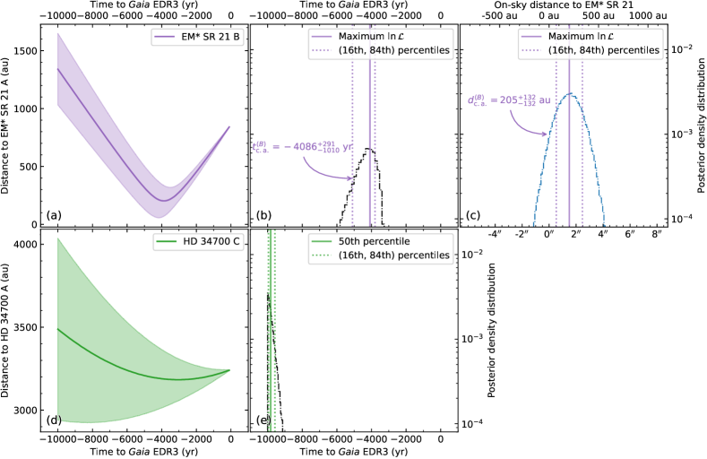
Figure 4: Relative distance as a function of past time for systems with recent close-in flyby events in Section 3.1. Top: Gaia DR3 6049152203067495808 (i.e., EM* SR 21 B) seen from EM* SR 21: moderate uncertainty growth in (a) allows for posterior calculation of the time of closest approach in (b), which shares the same vertical axis with the approach distance in (c). Bottom: Gaia DR3 3237512159787015936 (i.e., HD 34700 C) seen from HD 34700: uncertainty expansion in (d) cannot give conclusive answers to nearest approach time in maximum likelihood in (e), in which the MCMC samples drift towards the prior limit of $-10^{4}$ yr. Note: negative distances in (c) are physically implausible, yet it is the framework limit when sampling from normal distributions.

3.3 (Un)known binary systems

We did not identify flybys from neighbouring stars for the following systems, but they are (or could be) binary systems which have been (or should be) confirmed. What is more, the high RUWE measurements for certain systems suggest that the Gaia DR3 values could be biased due to the existence of binary companions. As a result, our linear framework that is fed with biased values cannot accurately trace the historical and future locations for these stars. To finalize flyby history for spiral formation mechanisms with high RUWE values, more reliable solutions from Gaia and a more realistic propagation framework are necessary.

3.3.1 AS 205

AS 205 is a binary system with the northern star AS 205 N hosting a pair of spirals in ALMA in Kurtovic et al. (2018), and the southern target AS 205 S being a spectroscopic binary. Gas emission between AS 205 N and AS 205 S shows tidal interaction between them, and the spirals surrounding AS 205 N could be explained by this (e.g., UX Tau: Ménard et al., 2020).

Among the 793 Gaia DR3 sources within $10$ pc from AS 205, 6 sources have their closest on-sky approach within the past $10^{4}$ yr, yet they are at least $86\sigma$ away from the spiral host. AS 205 S, however, will have a future closest approach of $d^{(f)}_{\rm c.a.}=183.3_{-1.6}^{+1.6}$ au at $t^{(f)}_{\rm c.a.}=+76.3$ yr. We do not identify recent close-in on-sky flyby candidates. However, the RUWE measurement for AS 205 is 1.75, indicating non-reliable solution from Gaia DR3 and compromising the corresponding linear flyby results.

3.3.2 HD 100453

HD 100453 is a binary system with a double spiral pattern in Wagner et al. (2015), with Dong et al. (2016) explaining the two spirals are driven by the companion HD 100453 B. Rosotti et al. (2020) observed CO gas connection to the companion in peak intensity using ALMA, which is consistent with the expectation that the spirals are driven by it.

The companion HD 100453 B is not reported in Gaia DR3. Among the 816 Gaia DR3 sources within $10$ pc from HD 100453, 10 sources have their closest on-sky approach within the past $10^{4}$ yr, among which Gaia DR3 5345034027626030848 had an on-sky distance $d^{(f)}_{\rm c.a.}=2767_{-1409}^{+1409}$ au (i.e., being $2\sigma$ away from zero separation) from the host at $t^{(f)}_{\rm c.a.}=-9740$ yr. Yet the rest of the 9 systems are at least $100\sigma$ away from the spiral host.

3.3.3 V599 Ori

V599 Ori shows a possible spiral in the SPHERE data. Among the 386 Gaia DR3 sources within $10$ pc from V599 Ori, 3 sources have their closest on-sky approach within the past $10^{4}$ yr, yet they are at least $5769\sigma$ away from the spiral host. We do not identify recent close-in on-sky flyby candidates.

The SPHERE data, however, shows a visually nearby source at $2\farcs 04$ to its northeast side. It matches the source Gaia DR3 3016081586083413120. Nevertheless, there is no parallax measurement for this source from Gaia DR3.

Given that Gaia DR3 3016081586083413120 situates along the pointing direction of the possible arm of V599 Ori, we cannot rule out it being a faint object that passed by the V599 Ori system. Future parallax and proper motion measurements is necessary to investigate the flyby relationship of the two sources.

4 Summary

Recent and close-in flyby of neighboring stars can excite short-lived spiral arms in protoplanetary disks. Assuming linear motion propagation and by developing an analytical framework afm-spirals (Shuai & Ren, 2022) and performing flyby analysis for 20 known spiral arm hosts resolved in polarized scattered light with VLT/SPHERE/IRDIS, we have identified EM* SR 21 as the only system with a plausible recent flyby candidate (EM* SR 21 B) responsible for the spirals. Nevertheless, existing evidences show that the EM* SR 21 system could be comprised of bounded objects, making the spirals instead probably resulting from companion-disk interaction.

For isolated systems that host spirals in scattered light, we have not identified recent and close-in flyby candidates from Gaia DR3 for them. This suggests that such flybys could not be the primary resources for the formation of spiral arms in scattered light for isolated systems. Should such objects exist, they are beyond the detection limits of Gaia DR3.

Moving forward, this framework can identify flyby candidates for new spiral systems, or establish flyby events when radial velocity measurements of comparable data quality are available. The flyby candidates from this framework do not require survey-level radial velocity observations, but discrete observations of individual targets. By doing so, we can reduce the observational cost in the search for stellar flyby events. Once these relationships are confirmed, however, we note that on the one hand, we cannot exclude the possibility that the spirals are indeed not excited by stellar flyby events. On the other hand, if stellar flyby events do have occurred, the orbits of the planets in these planet-forming systems could be excited to exotic orbits (e.g., Nguyen et al., 2021) that could be more challenging to image than those with circular orbits, which were previously assumed in spiral motion measurements (e.g., Ren et al., 2020; Xie et al., 2021; Safonov et al., 2022).

There are limitations in our study. First, we have only presented stellar flyby candidates that are identified in Gaia DR3 with both location and proper motion measurements. Second, we have adopted linear motion propagation in our flyby study, however this approach should be accurate for the purpose of identifying flyby events for isolated systems (e.g., De Rosa & Kalas, 2019). Third, for stars with moderate motion uncertainties – yet low accuracy – which thus cannot be identified to have statistically significant flyby, they could still be responsible for the excitement of spiral arms. Last but not least, the high RUWE terms in Gaia DR3 products for certain sources suggest biased measurements that could result into non-credible flyby events, and high RUWE values might indicate the existence of undetected companions which can drive the spirals. Nevertheless, when upcoming measurements with higher accuracy are available, our analytical framework will aid in narrowing down their connection to the observed spiral systems.

Appendix A Querying stars within $10$  pc

For each spiral host, we query the Gaia DR3 stars that are within its $10$ pc at https://gea.esac.esa.int/archive/, see the following Astronomical Data Query Language (ADQL) code which uses MWC 758 as a query example. In addition to the default results from any Gaia query, the ADQL outputs are used for our flyby analysis by including for each neighbor its angular on-sky distance to the host (“dist_arcsec”), distance to the Solar System (“z_pc”), and three-dimensional physical distance to the host (“dist_to_host”).

⬇

SELECT DISTANCE( POINT(’ICRS’, ra, dec), POINT(’ICRS’, 82.61472046369643, 25.332403978827056))*3600 AS dist_arcsec, -- Calculate on-sky angular distance to MWC 758

1000/gaiaDR3.gaia_source.parallax as z_pc, -- Convert parallax to distance in pc from Solar System

sqrt(power(155.87, 2)+power(1000/gaiaDR3.gaia_source.parallax, 2)-2*155.87*1000/gaiaDR3.gaia_source.parallax*cos(RADIANS(DISTANCE( POINT(’ICRS’, ra, dec), POINT(’ICRS’, 82.61472046369643, 25.332403978827056))))) as dist_to_MWC758, -- Calculate 3D distance to MWC 758

* FROM gaiaDR3.gaia_source

WHERE 1=CONTAINS( POINT(’ICRS’, ra, dec), -- Select neighbours within 10 pc from MWC 758 with 3 requirements below

CIRCLE(’ICRS’, 82.61472046369643, 25.332403978827056, 4)) and -- 1. Circling 11 pc on-sky sources from MWC 758, where 4deg = arctan(11pc/155.87pc) is calculated for MWC 758

(1000/gaiaDR3.gaia_source.parallax < 167) and -- 2a. Within 167 pc from Solar System

(1000/gaiaDR3.gaia_source.parallax > 144) and -- 2b. Beyond 144 pc from Solar System

(sqrt(power(155.87,2)+power(1000/gaiaDR3.gaia_source.parallax,2)-2*155.87*1000/gaiaDR3.gaia_source.parallax*cos(RADIANS(DISTANCE( POINT(’ICRS’, ra, dec), POINT(’ICRS’, 82.61472046369643, 25.332403978827056))))) < 10) -- 3. 3D distance to MWC 758 within 10 pc

ORDER BY dist_to_host ASC -- Order output stars by 3D distances to MWC 758

In the above ADQL query example, we increase the querying efficiency as follows. We first find the stars whose on-sky angular distances are within $11$ pc from MWC 758 to obtain a cone. We then identify those that have a distance that is within $10$ pc from the MWC 758 distance to the Solar System, thus segmenting the cone with concentric spheres. We finally select the stars that are within $10$ pc from MWC 758 in this segmented cone using the law of cosines, and order them by their three-dimensional distance to MWC 758. By doing so, the querying results can be obtained within $5$ min for each host.

Appendix B On-sky flyby framework

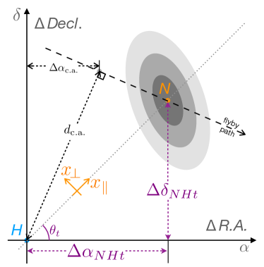
Figure 5: Sketch of bivariate normal distribution in B. Point $H$ is the position of spiral host in its reference frame (i.e., origin). Point $N$ is the relative location of a star neighbour seen from $H$, which is located at the center of the bivariate normal distribution in Equation (B4). The distribution along line $\overleftrightarrow{HN}$ is a one-dimensional normal distribution, see Equation (B13).

B.1 Relative position

The on-sky generalized coordinate (i.e., location and proper motion vector) of a star, $\bm{q}=(R.A.,Decl.,{\rm pm}_{R.A.},{\rm pm}_{Decl.})^{T}\triangleq(\alpha,\delta,\mu_{\alpha},\mu_{\delta})^{T}\in\mathbb{R}^{4\times 1}$ follows a four-dimensional multivariate normal distribution

$$\bm{q}\sim\mathcal{N}_{4}(\bm{\mu},\bm{\Sigma}),$$ (B1)

where $\triangleq$ is the symbol of definition, $\bm{\mu}=(\mathbb{E}\alpha,\mathbb{E}\delta,\mathbb{E}\mu_{\alpha},\mathbb{E}\mu_{\delta})^{T}\in\mathbb{R}^{4\times 1}$ contains the expected values from Gaia DR3, and $\bm{\Sigma}\in\mathbb{R}^{4\times 4}$ is the covariance matrix from Gaia DR3. Specifically, we divide the default Gaia output of $\mu_{\alpha^{*}}$ by $\cos{\delta}$ to obtain $\mu_{\alpha}$ (e.g., Squicciarini et al., 2021), and we modify the covariance matrix $\bm{\Sigma}$ similarly wherever applicable.

At time $t\in\mathbb{R}$, let

$$T_{t}=\begin{bmatrix}1&0&t&0\\ 0&1&0&t\end{bmatrix}$$ (B2)

be a transformation matrix, the on-sky position vector of the star, $\bm{x}_{t}=(R.A.,Decl.)^{T}\in\mathbb{R}^{2\times 1}$, is then

$$\bm{x}_{t}=T_{t}\bm{q} =\begin{bmatrix}1&0&t&0\\ 0&1&0&t\end{bmatrix}\begin{pmatrix}\alpha\\ \delta\\ \mu_{\alpha}\\ \mu_{\delta}\end{pmatrix}$$

$$=\begin{pmatrix}\alpha+t\mu_{\alpha}\\ \delta+t\mu_{\delta}\end{pmatrix}.$$ (B3)

Assuming a constant $\cos{\delta}$, $\bm{x}_{t}$ follows a bivariate normal distribution, $\bm{x}_{t}\sim\mathcal{N}_{2}(T_{t}\bm{\mu},T_{t}\bm{\Sigma}T_{t}^{T})$, where superscript ^T denotes matrix transpose.

The relative location of star neighbour $N$ from spiral host $H$ at time $t$, $\Delta\bm{x}_{NHt}=\bm{x}_{t}^{(N)}-\bm{x}_{t}^{(H)}\triangleq(\Delta\alpha_{NHt},\Delta\delta_{NHt})^{T}\in\mathbb{R}^{2\times 1}$ follows a bivariate normal distribution,

$$\Delta\bm{x}_{NHt}\sim \mathcal{N}_{2}\left(T_{t}\bm{\mu}^{(N)}-T_{t}\bm{\mu}^{(H)},T_{t}\bm{\Sigma}^{(N)}T_{t}^{T}+T_{t}\bm{\Sigma}^{(H)}T_{t}^{T}\right)$$

$$\triangleq\mathcal{N}_{2}\left(\bm{\mu}_{NHt},\bm{\Sigma}_{NHt}\right),$$ (B4)

where superscripts ^(H) and ^(N) denote the generalized coordinates for spiral host $H$ and its star neighbour $N$ from Equation (B1), respectively. See Figure 5 for an example of such a distribution at time $t$.

B.2 Statistical distribution

The statistical quantification of the relative location between two stars can be obtained along the direction of the two stars, i.e., along line $\overleftrightarrow{HN}$ in Figure 5. At time $t$, the functional form of Equation (B4) is fixed, and we can clockwise rotate the bivariate normal distribution by angle ${\theta_{t}}$ to align point $N$ along the horizontal axis. The rotation matrix for such a clockwise rotation is

$$R_{\theta_{t}}= \begin{bmatrix}\cos{\theta_{t}}&\sin{\theta_{t}}\\ -\sin{\theta_{t}}&\cos{\theta_{t}}\end{bmatrix},$$ (B5)

$$= \frac{1}{\sqrt{(\Delta\alpha_{NHt})^{2}+(\Delta\delta_{NHt})^{2}}}\begin{bmatrix}\Delta\alpha_{NHt}&\Delta\delta_{NHt}\\ -\Delta\delta_{NHt}&\Delta\alpha_{NHt}\end{bmatrix},$$ (B6)

where $\Delta\alpha_{NHt}=\left(\mathbb{E}\alpha^{\left(N\right)}-\mathbb{E}\alpha^{\left(H\right)}\right)+t\left(\mathbb{E}\mu_{\alpha}^{\left(N\right)}-\mathbb{E}\mu_{\alpha}^{\left(H\right)}\right)$, and $\Delta\delta_{NHt}=\left(\mathbb{E}\delta^{\left(N\right)}-\mathbb{E}\delta^{\left(H\right)}\right)+t\left(\mathbb{E}\mu_{\delta}^{\left(N\right)}-\mathbb{E}\mu_{\delta}^{\left(H\right)}\right)$.

The corresponding expression of the bivariate normal distribution after this rotation is

$$\Delta\bm{x}^{\prime}_{NHt}\triangleq\begin{pmatrix}x_{\parallel}\\ x_{\perp}\end{pmatrix}\sim \mathcal{N}_{2}\left(R_{\theta_{t}}\bm{\mu}_{NHt},R_{\theta_{t}}\bm{\Sigma}_{NHt}R_{\theta_{t}}^{T}\right)$$

$$=\mathcal{N}_{2}\left(R_{\theta_{t}}T_{t}\bm{\mu}^{(N)}-R_{\theta_{t}}T_{t}\bm{\mu}^{(H)},R_{\theta_{t}}T_{t}\bm{\Sigma}^{(N)}T_{t}^{T}R_{\theta_{t}}^{T}+R_{\theta_{t}}T_{t}\bm{\Sigma}^{(H)}T_{t}^{T}R_{\theta_{t}}^{T}\right)$$

$$\triangleq\mathcal{N}_{2}\left(\begin{bmatrix}\mu_{\parallel}\\ \mu_{\perp}\end{bmatrix},\begin{bmatrix}\sigma_{\parallel}^{2}&\rho\sigma_{\parallel}\sigma_{\perp}\\ \rho\sigma_{\parallel}\sigma_{\perp}&\sigma_{\perp}^{2}\end{bmatrix}\right),$$ (B7)

where $\mu_{\parallel}\in\mathbb{R}^{+}$, and $\rho\in[-1,1]$ is the correlation. The first element of $\Delta\bm{x}^{\prime}_{NHt}$, $x_{\parallel}$, corresponds to the distribution along line $\overleftrightarrow{HN}$, and the second element $x_{\perp}$ perpendicular to line $\overleftrightarrow{HN}$, see Figure 5.

Given the information of spiral host $H$ and a star neighbour $N$, the probability density distribution along line $\overleftrightarrow{HN}$ at time $t$, is therefore

$$x_{\parallel}\mid t\sim\mathcal{N}_{1}\left(\mu_{\parallel},\sigma^{2}_{\parallel}\right).$$ (B8)

B.3 Closest approach

In the reference frame of host $H$, the expected flyby path of star neighbour $N$ is a straight line, since the proper motion measurements are linearly propagated. The minimum distance between the two stars is thus the length of the line segment that is perpendicular to the flyby path of $N$, see Figure 5.

For $H$ and $N$, to obtain the analytical expressions of the closest approaches, here we define relative $R.A.$ offset in Gaia DR3 measurement as $\Delta\alpha=\alpha^{(N)}-\alpha^{(H)}$, relative $Decl.$ measurement $\Delta\delta=\delta^{(N)}-\delta^{(H)}$, relative proper motion along the $R.A.$ direction $\Delta{\mu_{\alpha}}=\mu_{\alpha}^{(N)}-\mu_{\alpha}^{(H)}$, and relative motion along the $Decl.$ direction $\Delta{\mu_{\delta}}=\mu_{\delta}^{(N)}-\mu_{\delta}^{(H)}$. Aligning the $R.A.$ direction with the $x$-axis and the $Decl.$ direction the $y$-axis in Cartesian coordinates, the flyby path can be expressed as

$$\frac{y-\Delta\delta}{x-\Delta\alpha}=\frac{\Delta\mu_{\delta}}{\Delta\mu_{\alpha}},$$

or

$$\Delta\mu_{\delta}\cdot x-\Delta\mu_{\alpha}\cdot y+\Delta\mu_{\alpha}\cdot\Delta\delta-\Delta\mu_{\delta}\cdot\Delta\alpha=0.$$ (B9)

Defining the functional form for the flyby path to be $ax+by+c=0$, and comparing with Equation (B9), then we have

$$\left\{\begin{matrix}a=&\Delta\mu_{\delta}\\ b=&-\Delta\mu_{\alpha}\\ c=&\Delta\mu_{\alpha}\cdot\Delta\delta-\Delta\mu_{\delta}\cdot\Delta\alpha\end{matrix}\right..$$ (B10)

The distance of the closest approach, or the length of the line segment that is perpendicular to the flyby path from $H$, is then

$$d^{(f)}_{\rm c.a.}=\frac{\left|\frac{c}{a}\right|\left|\frac{c}{b}\right|}{|c|\sqrt{\frac{1}{a^{2}}+\frac{1}{b^{2}}}}=\frac{|c|}{\sqrt{a^{2}+b^{2}}}.$$ (B11)

Focusing only on the horizontal direction, we can obtain the closest relative distance in the $R.A.$ direction,

$$\Delta\alpha_{\rm c.a.}=\frac{-{ac}}{{a^{2}}+{b^{2}}}.$$

Comparing the current – Gaia DR3 – relative distance in the $R.A.$ direction and the closest approach, we can obtain the time of closest approach analytically,

$$t^{(f)}_{\rm c.a.}=-{\frac{\Delta\alpha-\Delta\alpha_{c.a.}}{\Delta\mu_{\alpha}}}=-{\frac{\Delta\alpha+\frac{ac}{{a^{2}}+{b^{2}}}}{\Delta\mu_{\alpha}}},$$ (B12)

where negative value corresponds to closest approach in the past, while positive value in the future.

In our analysis, we calculate both the minimum expected on-sky distance and the time of the closest approach in Equations (B11) and (B12). We compare them with our criteria in both fly-by time ($-10^{4}$ yr $<t_{\rm c.a.}<0$), and distance of closest approach ($0<d_{\rm c.a.}<10r_{\rm disk}$, where $r_{\rm disk}$ is the radial extent of the spirals in existing observations), to select fly-by candidates. For the selected candidates, we calculate the posterior distribution and thus credible intervals as follows.

B.4 Posterior distribution

For the one-dimensional distribution along line $\overleftrightarrow{HN}$ in Equation (B8), the corresponding probability density function is

$$f(x_{\parallel}\mid H,N,t)=\frac{1}{\sqrt{2\pi}\sigma_{\parallel}}\exp\left[-\frac{(x_{\parallel}-\mu_{\parallel})^{2}}{2\sigma^{2}_{\parallel}}\right].$$ (B13)

For each star pair $H$ and $N$, the Gaia DR3 values can result into divergence of $\tan{\theta_{t}}$ in the calculation of $\theta_{t}$ for Equation (B5), since star $N$ can situate along the vertical axis in Figure 5 at some certain time $t$. In this study, we avoid this divergence by calculating the four matrix elements of Equation (B6) based on the definition of trigonometric functions using line segments.

B.4.1 Closest approach time

To obtain the posterior distribution for flyby times, we assume flat priors for the flyby times when $t\in[-10^{4},0]$ yr. We use emcee from Foreman-Mackey et al. (2013) to sample different flyby times $t$, and maximize the log-likelihood function corresponding to Equation (B13), i.e.,

$$\ln\mathcal{L}(t\mid H,N)=-\frac{1}{2}\left(\frac{x_{\parallel}-\mu_{\parallel}}{\sigma_{\parallel}}\right)^{2}-\ln\sigma_{\parallel}-\frac{1}{2}\ln(2\pi).$$ (B14)

For a given disk host $H$, we set $N$ to be one of its stellar neighbors and quantify the corresponding statistical significance of flyby using Equation (B8). We perform the likelihood calculation in Equation (B14) only for those candidate flyby neighbors to obtain the posterior distribution of their closest approach time $t^{(B)}_{\rm c.a.}$.

B.4.2 Closest approach distance

For candidates with well-constrained posterior distribution of closest approach time $t^{(B)}_{\rm c.a.}$, we obtain the posterior distribution of closest approach distance $d^{(B)}_{\rm c.a.}$ using both Glivenko–Cantelli theorem (e.g., Chung, 2001) and probability integral transform (Rosenblatt, 1952) as a proxy (e.g., Appendix B of Ren et al., 2019).

1. Obtain the empirical cumulative distribution function (ECDF) for the posterior distribution of the closest approach time $t^{(B)}_{\rm c.a.}$.

2. Sample a uniform distribution from 0 to 1, and match it to the ECDF value of $t^{(B)}_{\rm c.a.}$ to sample different closest approach time. The corresponding sample $t$ then follows the posterior distribution of closest approach time.

3. For each sample of $t$ from the posterior distribution, obtain the analytical expression of the host-neighbor separation from Equation (B8). Obtain one separation sample $d$ from the one-dimensional normal distribution.

4. Repeat Steps 2 and 3 for $10^{4}$ times, and obtain the posterior distribution for the closest approach distance $d^{(B)}_{\rm c.a.}$.

B.5 Generalizing framework for future measurements

For studies involving radial location and radial velocity from the Sun, a generalization of the framework here can be obtained by expanding the generalized coordinate $\bm{q}$ to a 6-element vector, adopting a $3\times 4$ transformation matrix in Equation (B2), and using a 3 dimensional rotation matrix in Equation (B5) such as in Gagné et al. (2018).

We do not generalize the framework here since the Gaia DR3 data do not have such complete information, and we leave it for a future study.

References

- Bae et al. (2018) Bae, J., Pinilla, P., & Birnstiel, T. 2018, ApJ, 864, L26
- Bae et al. (2016) Bae, J., Zhu, Z., & Hartmann, L. 2016, ApJ, 819, 134
- Bae et al. (2019) Bae, J., Zhu, Z., Baruteau, C., et al. 2019, ApJ, 884, L41
- Barsony et al. (2003) Barsony, M., Koresko, C., & Matthews, K. 2003, ApJ, 591, 1064
- Bisikalo et al. (2012) Bisikalo, D. V., Dodin, A. V., Kaigorodov, P. V., et al. 2012, Astronomy Reports, 56, 686
- Boccaletti et al. (2021) Boccaletti, A., Pantin, E., Ménard, F., et al. 2021, A&A, 652, L8
- Brittain et al. (2020) Brittain, S. D., Najita, J. R., Dong, R., & Zhu, Z. 2020, ApJ, 895, 48
- Cabrit et al. (2006) Cabrit, S., Pety, J., Pesenti, N., & Dougados, C. 2006, A&A, 452, 897
- Chung (2001) Chung, K. 2001, A Course in Probability Theory (Elsevier Science)
- Cuello et al. (2019) Cuello, N., Dipierro, G., Mentiplay, D., et al. 2019, MNRAS, 483, 4114
- Cuello et al. (2020) Cuello, N., Louvet, F., Mentiplay, D., et al. 2020, MNRAS, 491, 504
- Dai et al. (2015) Dai, F., Facchini, S., Clarke, C. J., & Haworth, T. J. 2015, MNRAS, 449, 1996
- de Boer et al. (2020) de Boer, J., Langlois, M., van Holstein, R. G., et al. 2020, A&A, 633, A63
- De Rosa & Kalas (2019) De Rosa, R. J., & Kalas, P. 2019, AJ, 157, 125
- Dohlen et al. (2008) Dohlen, K., Langlois, M., Saisse, M., et al. 2008, Proc. SPIE, 7014, 70143L
- Dong et al. (2018) Dong, R., Najita, J. R., & Brittain, S. 2018, ApJ, 862, 103
- Dong et al. (2016) Dong, R., Zhu, Z., Fung, J., et al. 2016, ApJ, 816, L12
- Dong et al. (2015) Dong, R., Zhu, Z., Rafikov, R. R., & Stone, J. M. 2015, ApJ, 809, L5
- Fabricius et al. (2021) Fabricius, C., Luri, X., Arenou, F., et al. 2021, A&A, 649, A5
- Fang et al. (2017) Fang, M., Kim, J. S., Pascucci, I., et al. 2017, AJ, 153, 188
- Foreman-Mackey et al. (2013) Foreman-Mackey, D., Hogg, D. W., Lang, D., & Goodman, J. 2013, PASP, 125, 306
- Furlan et al. (2009) Furlan, E., Watson, D. M., McClure, M. K., et al. 2009, ApJ, 703, 1964
- Gagné et al. (2014) Gagné, J., Lafrenière, D., Doyon, R., et al. 2014, ApJ, 783, 121
- Gagné et al. (2018) Gagné, J., Mamajek, E. E., Malo, L., et al. 2018, ApJ, 856, 23
- Gaia Collaboration et al. (2022) Gaia Collaboration, Vallenari, A., Brown, A. G. A., et al. 2022, arXiv, arXiv:2208.00211
- Gaia Collaboration et al. (2018) Gaia Collaboration, Brown, A. G. A., Vallenari, A., et al. 2018, A&A, 616, A1
- Herczeg & Hillenbrand (2014) Herczeg, G. J., & Hillenbrand, L. A. 2014, ApJ, 786, 97
- Kurtovic et al. (2018) Kurtovic, N. T., Pérez, L. M., Benisty, M., et al. 2018, ApJ, 869, L44
- Long et al. (2022) Long, F., Andrews, S. M., Zhang, S., et al. 2022, ApJ, 937, L1
- Ma et al. (2022) Ma, Y., De Rosa, R. J., & Kalas, P. 2022, AJ, 163, 219
- Malo et al. (2014) Malo, L., Doyon, R., Feiden, G. A., et al. 2014, ApJ, 792, 37
- Ménard et al. (2020) Ménard, F., Cuello, N., Ginski, C., et al. 2020, A&A, 639, L1
- Monnier et al. (2019) Monnier, J. D., Harries, T. J., Bae, J., et al. 2019, ApJ, 872, 122
- Muro-Arena et al. (2020) Muro-Arena, G. A., Ginski, C., Dominik, C., et al. 2020, A&A, 636, L4
- Nguyen et al. (2021) Nguyen, M. M., De Rosa, R. J., & Kalas, P. 2021, AJ, 161, 22
- Pfalzner (2003) Pfalzner, S. 2003, ApJ, 592, 986
- Pfalzner (2004) —. 2004, ApJ, 602, 356
- Pfalzner & Govind (2021) Pfalzner, S., & Govind, A. 2021, ApJ, 921, 90
- Prato et al. (2003) Prato, L., Greene, T. P., & Simon, M. 2003, ApJ, 584, 853
- Ren et al. (2018) Ren, B., Dong, R., Esposito, T. M., et al. 2018, ApJ, 857, L9
- Ren et al. (2019) Ren, B., Choquet, É., Perrin, M. D., et al. 2019, ApJ, 882, 64
- Ren et al. (2020) Ren, B., Dong, R., van Holstein, R. G., et al. 2020, ApJ, 898, L38
- Ren et al. (2021) Ren, B., Choquet, É., Perrin, M. D., et al. 2021, ApJ, 914, 95
- Riedel et al. (2017) Riedel, A. R., Blunt, S. C., Lambrides, E. L., et al. 2017, AJ, 153, 95
- Rodriguez et al. (2018) Rodriguez, J. E., Loomis, R., Cabrit, S., et al. 2018, ApJ, 859, 150
- Rosenblatt (1952) Rosenblatt, M. 1952, Ann. Math. Statist., 23, 470
- Rosotti et al. (2020) Rosotti, G. P., Benisty, M., Juhász, A., et al. 2020, MNRAS, 491, 1335
- Safonov et al. (2022) Safonov, B. S., Strakhov, I. A., Goliguzova, M. V., & Voziakova, O. V. 2022, AJ, 163, 31
- Shuai & Ren (2022) Shuai, L., & Ren, B. 2022, slinling/afm-spirals: pre-release v0.1, pre-release, Zenodo, doi: 10.5281/zenodo.7156158
- Squicciarini et al. (2021) Squicciarini, V., Gratton, R., Bonavita, M., & Mesa, D. 2021, MNRAS, 507, 1381
- Sterzik et al. (2005) Sterzik, M. F., Melo, C. H. F., Tokovinin, A. A., & van der Bliek, N. 2005, A&A, 434, 671
- Suárez et al. (2006) Suárez, O., García-Lario, P., Manchado, A., et al. 2006, A&A, 458, 173
- Takami et al. (2020) Takami, M., Beck, T. L., Schneider, P. C., et al. 2020, ApJ, 901, 24
- Uyama et al. (2020a) Uyama, T., Ren, B., Mawet, D., et al. 2020a, AJ, 160, 283
- Uyama et al. (2020b) Uyama, T., Currie, T., Christiaens, V., et al. 2020b, ApJ, 900, 135
- van Holstein et al. (2017) van Holstein, R. G., Snik, F., Girard, J. H., et al. 2017, Proc. SPIE, 10400, 1040015
- van Holstein et al. (2020) van Holstein, R. G., Girard, J. H., de Boer, J., et al. 2020, A&A, 633, A64
- Vigan et al. (2010) Vigan, A., Moutou, C., Langlois, M., et al. 2010, MNRAS, 407, 71
- Vincke & Pfalzner (2016) Vincke, K., & Pfalzner, S. 2016, ApJ, 828, 48
- Wagner et al. (2015) Wagner, K., Apai, D., Kasper, M., & Robberto, M. 2015, ApJ, 813, L2
- Xie et al. (2021) Xie, C., Ren, B., Dong, R., et al. 2021, ApJ, 906, L9
- Ygouf et al. (2019) Ygouf, M., Patel, R., Debes, J., et al. 2019, AAS Meeting, 233, 436.02
- Zhang et al. (2018) Zhang, S., Zhu, Z., Huang, J., et al. 2018, ApJ, 869, L47
- Zhu et al. (2011) Zhu, Z., Nelson, R. P., Hartmann, L., et al. 2011, ApJ, 729, 47