supplemental.pdf
Supercell low-level mesocyclones: Origins of inflow and vorticity
Abstract
The development of low-level mesocyclones in supercell thunderstorms has often been explained via the development of storm-generated streamwise vorticity along a baroclinic gradient in the forward flank of supercells. However, the ambient streamwise vorticity of the environment (often quantified via storm-relative helicity), especially near the ground, is particularly skillful at discriminating between nontornadic and tornadic supercells. This study investigates whether the origins of the inflow air into supercell low-level mesocyclones, both horizontally and vertically, can help explain the dynamical role of environmental versus storm-generated vorticity in the development of low-level mesocyclone rotation. Simulations of supercells, initialized with wind profiles common to supercell environments observed in nature, show that the air bound for the low-level mesocyclone primarily originates from the undisturbed, ambient environment, rather than from along the forward flank, and from very close to the ground, often in the lowest 200 - 400 m of the atmosphere. Given that the near-ground environmental air comprises the bulk of the inflow into low-level mesocyclones, this likely explains the forecast skill of environmental streamwise vorticity in the lowest few hundred meters of the atmosphere. The low-level mesocyclone does not appear to require much augmentation from the development of additional horizontal vorticity in the forward flank. Instead, the dominant contributor to vertical vorticity within the low-level mesocyclone is from the environmental horizontal vorticity. This study hopefully clarifies the development of low-level mesocyclones in supercells.
Supercell thunderstorms produce the majority of tornadoes, and a defining characteristic of supercells is their rotating updraft, known as the “mesocyclone”. When the mesocyclone is stronger at lower altitudes, the likelihood of tornadoes increases. The purpose of this study is to understand if the rotation of the mesocyclone in supercells is due to horizontal spin present in the ambient environment or whether additional horizontal spin generated by the storm itself primarily drives this rotation. Our results suggest that inflow air into supercells, and low-level mesocyclone rotation, is mainly due to the properties of the environmental inflow air, especially near the ground. This hopefully will clarify how our community views the development of low-level mesocyclones in supercells.
1 Introduction
A defining characteristic of supercell thunderstorms is their mesocyclone, a quasi-steady region of vertical vorticity within the storm’s updraft. This persistent feature contributes to the supercell’s ability to produce a host of severe weather threats, including damaging nontornadic winds (Smith et al., 2012), flash flooding (Nielsen and Schumacher, 2020), large individual hail stones (Blair et al., 2017) and/or large accumulations of small hail (Kumjian et al., 2019), and tornadoes (Markowski and Richardson, 2009). Conceptual models of supercells have all prominently featured the mesocyclone (Brandes, 1978; Lemon and Doswell, 1979; Klemp, 1987; Doswell and Burgess, 1993), and temporal increases in mesocyclone rotation near the cloud-base have long been identified as a precursor of tornadoes (e.g., Brandes, 1993; Burgess et al., 1993; Thompson et al., 2017). Despite these connections between mesocyclones and tornadoes, the presence of a mesocyclone alone is a poor predictor of supercellular tornadogenesis (Trapp, 1999). Although most tornadoes are associated with supercells, perhaps less than 15% of mesocyclones are tornadic (Trapp et al., 2005; Smith et al., 2012).
The process of supercellular tornadogenesis is often described as having three steps (Davies-Jones, 2015). First, an updraft needs to require rotation aloft (i.e., the development of a mesocyclone). It is well established that the updrafts of supercells initially acquire their rotation via the tilting of horizontal vorticity associated with the vertical shear of the environmental wind profile (e.g., Rotunno and Klemp, 1982; Davies-Jones, 1984; Weisman and Rotunno, 2000). Specifically, the tilting of streamwise horizontal vorticity (i.e., the component of vorticity aligned parallel to the motion of air in the storm-relative framework) is a necessary requirement for the updraft to acquire net positive vertical vorticity (Davies-Jones, 1984, 2017, 2022; Dahl, 2017).
The second step in tornadogenesis involves rotation developing at the ground. Surface vertical vorticity is thought to occur primarily through some combination of baroclinic (e.g., Davies-Jones, 1982; Davies-Jones and Brooks, 1993; Walko, 1993; Adlerman et al., 1999; Dahl et al., 2014; Markowski and Richardson, 2014; Dahl, 2015; Parker and Dahl, 2015) and frictional (e.g., Schenkman et al., 2014; Markowski, 2016; Mashiko, 2016; Roberts et al., 2016; Yokota et al., 2018; Fischer and Dahl, 2022b) generation of horizontal vorticity within downdrafts. Following generation, this horizontal vorticity is subsequently tilted into the vertical very close to the surface (Rotunno et al., 2017), typically in cyclonically curved, descending air parcels embedded in the rear-flank outflow near the tip of the hook echo (Davies-Jones, 2022).
Both nontornadic and tornadic supercells readily acquire this sub-tornadic rotation near the surface (Parker and Dahl, 2015; Coffer et al., 2017). Hence, steps 1 and 2 are necessary, but not sufficient, for tornadogenesis. The third and final step in tornadogenesis is the contraction and intensification of coherent areas of large circulation at the ground into a tornadic strength vortex (e.g., Parker, 2023). For this to occur, several conditions apparently need to be met simultaneously. The sub-tornadic rotation needs be within outflow air that has sufficiently small negative buoyancy so that it does not resist upward acceleration into the low-level updraft (Markowski et al., 2002). Surface rotation also must experience persistent convergence and stretching. Because this is necessarily below the height of the LFC (where air is either neutrally or negatively buoyant), the bulk of the associated vertical accelerations must be provided by the mesocyclone and its associated dynamic lifting (Rotunno and Klemp, 1982; Lilly, 1986; Markowski et al., 2012b; Markowski and Richardson, 2014; Coffer and Parker, 2015, 2017; Goldacker and Parker, 2021)111In low LCL environments common to tornadic supercells, buoyant vertical pressure perturbation gradients can also have a slight upward contribution to the total acceleration field (Brown and Nowotarski, 2019, see their Fig. 14).. This dynamic lifting owes its existence to pressure falls aloft associated with the mesocyclone’s circulation. Many studies use the 0 - 1 km vertical perturbation pressure gradient acceleration as a measure of this dynamic lifting provided by the mesocyclone. In addition, tornadogenesis is more likely when there is a vertical alignment of the near-ground, low-level, and mid-level rotation (Snook and Xue, 2008; Guarriello et al., 2018), which can be affected by the distribution of shear (Markowski and Richardson, 2014; Gray and Frame, 2021), the storm-relative flow (Brooks et al., 1994; Warren et al., 2017), properties of the outflow and surges (Skinner et al., 2014; Marquis et al., 2016), as well as the distribution of negative buoyancy (Markowski and Richardson, 2017) and hydrometeors (Loeffler et al., 2020).
Within this chain of processes, the point at which a supercell ultimately succeeds or fails in producing a tornado appears is strongly linked to the mesocyclone, specifically the rotation in the lower troposphere (Thompson et al., 2017). Hence, low-level mesocyclone intensity exerts a substantial influence on tornadogenesis likelihood (e.g., Markowski and Richardson, 2014; Coffer and Parker, 2017; Peters et al., 2023). We will refer to the mesocyclone near cloud-base as the “low-level” mesocyclone [in the lower troposphere at approximately 1 km above ground level (AGL)] and consider this level distinct from both the “mid-level” mesocyclone further aloft (in the mid-troposphere between 3-6 km AGL) and the “near-ground” rotation that develops much closer to the surface ( 250 m AGL, sometimes referred to as the “tornado cyclone”). While rigid distinctions between these levels can be somewhat problematic (as discussed in Markowski et al., 2008, Section 4c), especially at later stages in supercell lifecycles and immediately preceding tornadogenesis, we distinguish the low-level mesocyclone in this way because it is this altitude range where rotation is responsible for the dynamic upward accelerations that must occur below the LFC to produce tornadogenesis.
Current thinking regarding the mesocyclone at low-levels largely originates from the seminal modeling work of Rotunno and Klemp (1985). By integrating material circuits backward from an area of low-level rotation, Rotunno and Klemp (1985) showed that it was linked to an “upward tilting of baroclinically-generated horizontal vorticity along the cool air boundary situated upstream of the low-level updraft”. The orientation of the forward-flank baroclinic zone and the storm-relative flow in this region of the storm is such that baroclinically-generated vorticity is predominantly streamwise (Klemp and Rotunno, 1983). In simulations with and without rain, rotation in the mid-levels developed consistently through the tilting of environmental horizontal vorticity. On the other hand, low-level rotation was absent in simulations without rain. The Rotunno and Klemp (1985) analysis was performed at the lowest model level (250 m AGL), so there is some ambiguity about whether the “low-levels” they described are more applicable to the the low-level mesocyclone rotation near cloud-base (as-in this work) or the origins of surface rotation (as-in Davies-Jones and Brooks, 1993). In either case, Rotunno and Klemp (1985) has become the defacto reference used to explain the development of low-level mesocyclones (e.g., Markowski et al., 1998; Atkins et al., 1999; Wakimoto and Cai, 2000; Markowski et al., 2003b; Shabbott and Markowski, 2006; Orf et al., 2017; Frank et al., 2018; Markowski, 2020; Fischer and Dahl, 2020; Flournoy et al., 2020, 2021; Murdzek et al., 2020b, a; Schueth et al., 2021; Davies-Jones, 2022; Finley et al., 2023).
In one of the most well-observed supercells in history, Markowski et al. (2012b) used a dual-Doppler wind syntheses to show that as much as 70-90% of the low-level mesocyclone (at 750 m AGL) was due to storm-generated sources. Other observations also seem to point to forward-flank processes as fundamental to low-level mesocyclones. Circumstantial evidence includes visual cues in low-level cloud features, such as a localized lowering of the cloud base (the “wall cloud”, often tilted towards the region of forward flank precipitation; Fujita, 1957; Atkins et al., 2014) due to the influx of precipitation-cooled air into the low-level mesocyclone area. Additionally, vortex lines around mesocyclones from Doppler radar studies are often configured into ‘vortex line arches’, which are highly suggestive of upward tilting of baroclinically generated horizontal vorticity within the low-level mesocyclone (e.g., Straka et al., 2007; Markowski et al., 2008, 2012a). Markowski and Richardson (2010) thus summarize the current understanding: “the formation of low-level mesocyclones usually awaits the development of an extensive forward-flank precipitation region and outflow” because the “tilting of the baroclinically enhanced low-level horizontal vorticity produces more significant vertical vorticity at low altitudes than does the tilting of environmental vorticity alone”.
Attention to this concept has been revived by recent interest in the “streamwise vorticity current” (SVC; Orf et al., 2017), a localized region of horizontal streamwise vorticity located parallel to the forward flank outflow boundary. Analyzing a very high-resolution simulation of an EF5 tornadic supercell, Orf et al. (2017) stated that the SVC was ingested into the storm’s updraft, intensifying the low-level mesocyclone, and leading to the amplification and maintenance of a long-lived violent tornado. This correlation between the intensifying SVC and low-level mesocyclone was expanded upon by Finley et al. (2023). While the idea of storm-generated, streamwise horizontal vorticity production within the forward flank has previously been discussed in the literature (as reviewed above), the unprecedented level of detail in these simulations has inspired subsequent exploration in a number of modeling studies (Markowski, 2020; Schueth et al., 2021) and observed cases (Markowski et al., 2018; Murdzek et al., 2020a, b; Schueth et al., 2021), and has been an explicit emphasis in recent field projects (Weiss et al., 2020).
Even so, it appears that not all supercells have SVCs, and the presence (or lack) of an SVC is not a necessary requirement for tornadogenesis success (or failure; Murdzek et al., 2020a). Even when an SVC is present, it is not guaranteed that the augmented, storm-generated streamwise horizontal vorticity within this feature ends up participating in the low-level mesocyclone (Murdzek et al., 2020b). It seems that substantial uncertainty remains. The present study inherits the question asked by Markowski et al. (2012b): “is large environmental vorticity important, especially at low-levels, because its tilting establishes the base of the mid-level mesocyclone at fairly low elevations?” Indeed, there is accumulating evidence that tornadic environments are distinguished by large environmental streamwise vorticity in the lowest 500 - 1000 m AGL (Markowski et al., 2003a; Rasmussen, 2003; Miller, 2006; Esterheld and Giuliano, 2008; Nowotarski and Jensen, 2013; Parker, 2014; Coffer et al., 2019, 2020; Nixon and Allen, 2022). And, a number of modeling studies have attributed the mesocyclone’s strong dynamic lifting in the lower troposphere to this environmental source (Markowski and Richardson, 2014, 2017; Coffer and Parker, 2017; Goldacker and Parker, 2021; Peters et al., 2023).
The vertically integrated storm-relative flux of streamwise vorticity into an updraft, represented by the storm-relative helicity (SRH), is of the greatest dynamical importance in this regard (Davies-Jones, 1984). SRH must be defined over a layer of some depth, and the choice of this depth is non-trivial. Some studies have attempted to define an inflow layer based on thermodynamic properties such that only parcels associated with CAPE and minimal CIN are included (the effective inflow layer or EIL; Thompson et al., 2007; Nowotarski et al., 2020). However, model-based proximity soundings show that SRH very near the ground (e.g., 0 - 500 m AGL; SRH500) is the single most predictive parameter in discriminating significantly tornadic supercells from their nontornadic counterparts, in both United States and European severe weather environments (Coffer et al., 2019, 2020). In a pair of simulated supercells (one tornadic, one nontornadic), Coffer and Parker (2017) showed that the environmental inflow parcels bound for the low-level mesocyclone originated exclusively below 300 m AGL. However, the sources of air bound for the low-level mesocyclone across a range of supercells in various environments has not yet been systematically evaluated.
There is ambiguity in the previous literature concerning the role of environmental versus storm-generated vorticity in the production and maintenance of low-level mesocyclones. Several prominent conceptual models [e.g., Markowski et al. (2008), their Fig. 19, and Rotunno et al. (2017), their Fig. 1] seem to depict the low-level and mid-level mesocyclones as sourced from distinct air streams. Some authors have suggested that the low-level mesocyclone is primarily attributable to storm-generated baroclinic processes (e.g., Finley et al., 2023), while others have argued that the storm-generated vorticity merely augments the environmental contribution (e.g., Markowski and Richardson, 2010). This uncertainty about the importance of environmental versus storm-generated vorticity in low-level mesocyclone development leads us to our main research questions:
-
1.
If low-level mesocyclone-genesis is primarily attributable to storm-generated, forward flank baroclinic generation of horizontal vorticity, then why is near-ground environmental streamwise vorticity such a highly skillful forecast parameter?
-
2.
How much augmentation, if any, to the low-level mesocyclone from storm-generated horizontal vorticity is necessary to modulate the intensity of low-level dynamic lifting that ultimately can determine whether a supercell fails or succeeds at producing a tornado?
To address these questions, we explore the origins and properties of air parcels that end up in the low-level mesocyclone using a matrix of simulations initialized with wind profiles common to supercell environments observed in nature and representing a spectrum of near-ground horizontal vorticity magnitudes and orientations.
2 Methods
2.1 CM1 model
Supercell simulations were performed using Cloud Model 1 (CM1; Bryan and Fritsch, 2002) release 20.3. Storms were simulated for 3 h on a 200 200 18 km3 domain with a horizontally homogeneous environment (described in Section 2b). The inner 100 x 100 km2 had a horizontal grid-spacing of 80 m during the period of analysis, while the vertical grid-spacing was stretched from 20 m in the lowest 300 m to 280 m at 12 km. The domain was translated with a constant storm-motion, which was determined iteratively by trial and error to keep the storm approximately centered within the domain. A fifth-order advection scheme, utilizing high-order-weighted essentially nonoscillatory finite differencing, was used with no additional artificial diffusion (Wicker and Skamarock, 2002). The subgrid-scale turbulence was parameterized by a 1.5-order turbulence kinetic energy closure scheme similar to Deardorff (1980), with separate horizontal and vertical turbulence coefficients. Open-radiative lateral boundary conditions were employed, and where there was an inward mass flux into the domain, the horizontal winds were nudged back towards the base-state fields along the lateral boundaries (i.e., in the namelist). The upper-boundary had a rigid, free-slip boundary condition, with a Rayleigh damping sponge applied above 14 km, while the bottom boundary condition was semi-slip with a constant surface drag coefficient () of 0.0035 to partially capture frictional effects on within-storm processes. The was calculated using the surface layer scheme by Jiménez et al. (2012) based on the thermodynamic profile and the mean of the kinematic profiles discussed in Section 22.2. Random perturbations of 0.25 K were added to the initial conditions within the lowest 1000 m AGL. The simulations use a six-category, fully double-moment bulk microphysics scheme from the National Severe Storms Laboratory (NSSL) that explicitly predicts the variable densities of hail and graupel (Ziegler, 1985; Mansell, 2010; Mansell et al., 2010). Convection is initialized using the heat flux method of Carpenter et al. (1998) and Lasher-Trapp et al. (2021) and is described in more detail below.
2.1.1 Heat flux convective initialization
We used a Gaussian heat flux based on Lasher-Trapp et al. (2021) and similar to Morrison et al. (2022), that results in a more natural transition from buoyant plumes to a sustained, mature supercell updraft across all the environments used herein (Peters et al., 2022a, b). The heat flux was strongest near the surface and exponentially decreased in magnitude radially and vertically. The horizontal width and height of the Gaussian function were 10000 and 2500 m, respectively. The heat flux linearly ramps up from 0 to 2000 W m-2 over the first minute of the simulation. This amplitude was maintained for 28 min, then linearly decreased back to zero over 1 min, for a total of 30 min of active heating. In addition to the heating, a very weak Gaussian-shaped forced convergence [(10-4)] was applied to the horizontal wind field over the same spatial and temporal dimensions of the surface heating (similar to Moser and Lasher-Trapp, 2018). The combined effect of surface heating and weak convergence resulted in initially shallow thermal-like updrafts that gradually transitioned into a sustained steady supercell updraft (Peters et al., 2022a, b). While the convection organically developed during the first hour of the simulation, the horizontal grid-spacing of the simulation within the inner 100 100 km2 was 250 m, which Lasher-Trapp et al. (2021) found suitable for simulating overturning circulations and entrainment. Afterwards, the horizontal grid-spacing within the inner domain was decreased to 80 m, as discussed next.
2.1.2 Downscaling to finer grid-spacing
To adequately resolve features important to the development and maintenance of the low-level mesocyclone and tornadoes, the horizontal grid-spacing within the inner domain of the simulations was downscaled to 80 m an hour into the simulation using the technique of Coffer and Parker (2022). The vertical grid-spacing was unchanged. Downscaling was accomplished by fitting a unique gridded interpolation function (cubic spline) to each two- and three-dimensional array in the model’s restart file, essentially creating a one-way nest within CM1.
For comparison, the original 250 m simulations were also run for the full 3 h. Generally the supercells evolved qualitatively similarly between the original 250 m and downscaled 80 m simulations. Subjective comparisons between both resolutions showed that no simulation that produced a tornado-like vortex at 250 m became nontornadic in the 80 m simulation (and vice-versa). The similarities at different resolutions may be somewhat surprising given the low degree of intrinsic predictability within supercells (Markowski and Richardson, 2017; Markowski, 2020); however, it appears, based on the these results, that most of the spread in predictability occurs within the convection initiation and development phase (similar to predictability challenges in operational convective forecasting, e.g., Galarneau et al., 2022).
2.2 Kinematic and thermodynamic base-state environments
To best encompass a range of wind profiles with varying magnitudes of near-ground SRH observed in nature, self-organizing maps (SOMs) were used to identify recurring low-level wind profile patterns from 20,194 model-analyzed supercell proximity soundings previously analyzed by Coffer et al. (2019). SOMs have previously been used to identify recurring features in severe weather datasets (Nowotarski and Jensen, 2013; Anderson-Frey et al., 2017; Nowotarski and Jones, 2018; Warren et al., 2021; Hua and Anderson-Frey, 2022). The SOMs were trained on the 0 - 500 m AGL ground-relative u,v wind components, similar to Goldacker and Parker (2021). The 0 – 500 m AGL layer was selected because it represented the most distinct layer between significantly tornadic and nontornadic supercells in Coffer et al. (2019). All soundings were interpolated to a common vertical grid with 50 m grid-spacing. Training was conducted with three nodes in both the direction, using a learning rate of 0.1 and iterated over 10,000 training steps. Wind profiles with layers of anti-streamwise vorticity within the lowest 500 m AGL were excluded, leaving a total of 15,906 of cases used in the SOM training. The cases removed represent environments that are not conducive to low-level mesocyclone development and were predominately associated with nontornadic supercells. While SOMs have many uses, the intention herein was to distill a large dataset of environmental soundings into a handful of archetypal hodographs to initialize a reasonable number of supercell simulations for analysis.
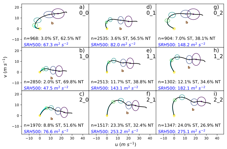
The resulting nine wind profiles from the SOM vary the magnitude and orientation of the near-ground hodograph (Fig. 1), generally increasing the magnitude of 0 - 500 m AGL vertical wind shear vector from left to right and shifting the direction of the shear vector from southwesterly to southerly from top to bottom (Fig. 1). All profiles have at least 20 m s-1 of 0 - 6 km bulk vertical wind shear, supportive of supercells. SRH500 increases from 50 m2 s-2 in node 1_0 to 275 m2 s-2 in node 2_2. Each ground-relative wind profile from the SOM was subsequently shifted to the origin of the hodograph at the lowest model level (i.e., no surface wind). Shifting the wind profile minimizes the influence of the semi-slip bottom boundary condition on the wind profile over the course of the 3 h simulation without introducing unnatural, or invented, forces into the model’s equation set (Davies-Jones, 2021). The wind profile was also run through a 1 h CM1 single-column simulation in order to let the profile adjust to the semi-slip bottom boundary condition. Differences were essentially nonexistent between the initial, adjusted, and final far-field wind profile after the 3 h simulation.
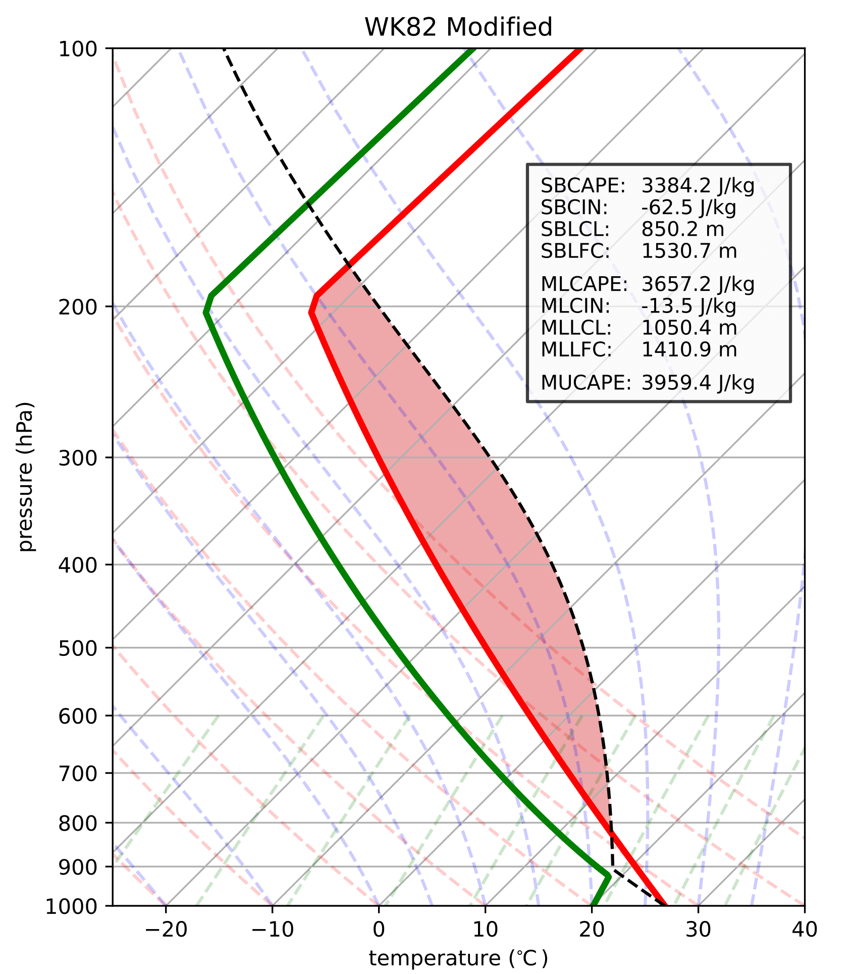
Each kinematic profile from the SOM was paired with the same thermodynamic profile (Fig. 2) in order to isolate the influence of the wind profile on the development of low-level mesocyclones. A modified version of the Weisman and Klemp (1982) sounding was used to generate potential temperature and relative humidity profiles. The modifications are the same as those described by Markowski (2020) and are designed to minimize the appearance of moist absolutely unstable layers and unwanted/uncontrolled convection initiation. Mixed-layer CAPE is 3657 J kg-1, CIN is -14 J kg-1, the LCL is approximately at 1050 m AGL, the LFC is near 1500 m AGL, and the top of the EIL is 2700 m AGL (Fig. 2). All parameters were calculated as-in Coffer et al. (2019). These bulk thermodynamic quantities represent the upper-end of the supercell spectrum, and are more similar to the subset of significantly tornadic supercells than to nontornadic supercells in the Coffer et al. (2019) dataset.
2.3 Analysis techniques
2.3.1 Mesocyclone tracking and definition
To objectively analyze each supercell, the mesocyclone was tracked over time. The algorithm tracked the peak of a Gaussian, spatially smoothed product of vertical velocity and vertical vorticity (of at least 0.01 s-1) at 1 km AGL (Werkema, 2022). A temporally smoothed time series of mesocyclone centroids was then computed using a 3rd order polynomial, Savitzky-Golay filter with an 11 point window (i.e., 5 minutes of output). This method reliably tracked the right-moving supercell of interest in each simulation bar one. Simulation 1_0, which had the smallest near-ground SRH and weakest storm-relative flow, experienced multiple splits and the right-moving storm began to dissipate two hours into the simulation. For this reason, a subjectively defined right moving updraft area was instead defined for the simulation 1_0 during a key period of interest (i.e., before the storm began to dissipate).
For analysis purposes, the low-level mesocyclone in each supercell was defined as the grid points at 1 km AGL with vertical vorticity values of at least 0.01 s-1 and vertical velocities that exceeded the 90th percentile (Table 1) within a 10 km diameter of the tracked mesocyclone centroids. In other words, the vertical velocity and vertical vorticity thresholds isolate the portion of the low-level mesocyclone in each supercell that contains up the most intense upward-moving, cyclonically rotating air and thus the greatest potential for vertical stretching (i.e., largest , which is highly correlated with dynamic lifting, Goldacker and Parker, 2021). We chose an altitude of 1 km AGL, near cloud-base for most supercells, not only because mesocyclonic rotation is responsible for upward dynamic accelerations below the LFC (as discussed previously), but also because there is a distinct local maximum in the vertical vorticity field at approximately 1 km AGL across the matrix of simulations presented herein (discussed later). Much of the analysis presented herein was rerun varying the definition of the low-level mesocyclone, including no vertical vorticity requirement, lowering the altitude for what was considered “low-level” (i.e., 500 and 750 m AGL), using lower (and higher) thresholds of vertical velocity at 1 km AGL (i.e., the 50th and 99th percentiles), as well as defining the low-level mesocyclone as a coherent area of positive circulation. None of these modifications produced an appreciable change in the overall conclusions.
2.3.2 Key time periods tornado-genesis/failure
In order to analyze supercells at similar points in their evolution, a key time period of tornadogenesis or tornadogenesis failure was determined for each simulation. Similar to the definitions of Coffer et al. (2017), vortices at 10 m AGL (i.e., the lowest bottom model level) were considered tornadoes if they met the following criteria: 1) vertical vorticity 0.3 s-1 2) a pressure drop -10 hPa throughout the lowest 1 km, and 3) a ground-relative wind speed 29 m s-1 (i.e., the EF-0 threshold) within 1 km of the position of maximized Okubo-Weiss (OW) parameter ( ). All three criteria needed to be satisfied for at least two minutes. If these thresholds were not met at any time during a simulation, tornadogenesis failure was defined as the time of maximum OW at 10 m AGL within a 10 km diameter of the tracked low-level mesocyclone centroid point.
2.3.3 Tracers and backward trajectories
To visualize the source regions of the low-level mesocyclone, three layers of passive tracers were initialized in CM1 [0 - 500 m AGL, 500 - 1500 m AGL (the approximate height LFC), and 1500 - 2700 m AGL (the top of the EIL)], which were advected within the simulation during integration. The value of the tracer mass mixing ratio in each layer was initially set to 1. In addition to tracers, backward trajectories were used to determine source regions of the low-level mesocyclone with a finer level of spatial detail than tracers can provide. The method of integrating backward trajectories loosely followed that of Gowan et al. (2021), except that between native output intervals (60 s), velocity fields were linearly interpolated into 3 s intervals to ensure that trajectories do not “skip” over entire grid cells during a single integration step. Backward trajectories were initialized at grid points within the defined low-level mesocyclone every 60 s between 5 and 10 minutes prior to the key time period of tornado-genesis/failure ( to ) and were tracked backwards for 30 mins, allowing the final position of the trajectories to be far enough removed from the storm. Given that the timescale for tornado formation is roughly 10 mins (Davies-Jones et al., 2001), the to time window focuses on the point within the low-level mesocyclone’s evolution in which the tornadogenesis process is ongoing, not at when a tornado has potentially already formed222Backward trajectories in the to post-tornadogenesis time frame have a very similar shape, width, and depth to the pre-tornadogenesis trajectories presented herein. Many of the trajectories in the minutes immediately preceding tornadogenesis ( to ) resemble trajectories that result in near-ground rotation from Dahl et al. (2014), Dahl (2015), and Fischer and Dahl (2020) within downdrafts in the rear-flank outflow before swiftly rising into the low-level mesocyclone.. This eludes the potentially problematic issue of determining the exact moment surface rotation should be considered “tornadic” (e.g., Houser et al., 2022).
2.3.4 Material stencils
In order to address the relative contributions of environmental versus storm-generated horizontal vorticity upon the mesocyclone, we complement the tracer and backward trajectory analysis with forward trajectories within CM1. Using the “material stencil” method from Dahl et al. (2014) and Dahl and Fischer (2023), the initial (or “imported”) environmental vorticity of a parcel can be separated from the contribution of vorticity generated by the storm. Following Dahl et al. (2014), six additional adjacent stencil parcels were initialized surrounding a center parcel at distances of 0.5 m. Over time, the stencils are deformed, and the embedded initial vorticity vector is reoriented accordingly (behaving as a material fluid that is tilted and stretched). Thus, for parcels that subsequently enter the low-level mesocyclone, the component of the vertical vorticity that is due to the initial ambient vorticity can be derived based on the final configuration of the stencil. The storm-generated component is simply the residual between the known vorticity at some final time and the rearranged initial vorticity component.
Since the initial parcel locations may not be representative of completely undisturbed base-state air due to far-reaching storm influences on the environment (e.g., Parker, 2014; Wade et al., 2018; Coniglio and Parker, 2020), we extended the stencil method from Dahl et al. (2014) to parse out two components of initial vorticity. The initial stencil vorticity vectors include both the base-state values from model initialization () and any perturbations that have developed between the model start time and the stencil initialization time (). Therefore the final vertical vorticity () of the low-level mesocyclone () is
| (1) |
where is the component of the initial stencil vorticity that is rearranged by the storm via tilting and stretching, divided into the base-state environment () and pre-existing perturbations (), and is the residual storm-generated component that contains all the nonconservative vorticity production processes, such as baroclinic, subgrid-scale mixing, and diffusion (and the eventual rearrangement of those nonconservative processes). Both base-state environment () and pre-existing perturbations () are treated as ‘frozen to the flow’ and can be rearranged via tilting and stretching. Because it is unknown whether or not represents a prior process that represents a rearrangement of the initial environmental vorticity vector or vorticity produced by the storm itself, the three components of will be reported separately. The total of and always sums to , which is what was originally presented in Dahl et al. (2014). We hope that separating the base-state and perturbation vorticity vectors in this manner helps to address historical concerns that analyzed trajectories were potentially not fully removed from the storm’s influence at the time of initialization.
Forward trajectories were seeded within model restart files 40 minutes before the key time period of tornado-genesis/failure for each simulation and integrated forward natively within CM1 for 35 minutes. This results in parcels with at least 30 minutes of output history during the same five minute composite period ( to ) highlighted by the backward trajectories. Horizontally, parcels were launched upstream of the low-level mesocyclone within a unique horizontal bounding box for each simulation encompassing an estimated 75% of the low-level mesocyclone inflow area based on the backward trajectories, with a 2 km buffer upstream in the , , and directions (to account for potential errors in backward trajectories). Vertically, parcels were defined over a 1500 m layer starting at 30 m AGL (i.e., the second lowest model level333The second lowest model level was the lowest chosen because surface drag always opposes the local wind field at the lowest model grid point with a “semi-slip” bottom-boundary condition, yielding questionable horizontal vorticity fields (i.e., Wang et al., 2020, 2023).), except for the 1_0 simulation where parcels were extended up to 2000 m due to higher parcel origin heights (shown later). The center stencil parcels were defined on an isotropic 100 m grid within the bounding box, with the six adjacent stencil parcels initialized surrounding each center parcel at distances of 0.5 m. Each simulation had between 2,000,000 and 12,000,000 total forward trajectories, depending on the areal extent of the inflow and thus the size of the bounding box (shown later). Parcel data were saved every 15 s and low-level mesocyclone trajectories were identified using the same thresholds as the backward trajectories, i.e., vertical velocity greater or equal to the 90th percentile (Table 1) and at least 0.01 s-1 of vertical vorticity (within 10 m of 1 km AGL).
3 Results
3.1 General characteristics of the simulations
All nine wind profiles from the SOM resulted in supercellular convection for the majority of the 3 hour simulation time. Eight of the nine simulations develop quasi-steady, right-moving supercells with persistent (and trackable) low-level mesocyclones of varying intensity (Fig. 3). The lone exception is simulation 1_0, which due to the lack of curvature and storm-relative flow in the hodograph (Fig. 1b), experiences a succession of splits. After two hours, only disorganized multi-cell convection exists throughout the domain in simulation 1_0 and peak vertical velocities drop off substantially compared to the other eight simulations (Fig. 4a). Despite the unsteady nature, at times, the southern-most, right-moving storm in simulation 1_0 periodically displays supercellular features in the reflectivity field, such a hook echo444The most prominent of such instances is chosen as the key time period and the centroid of the low-level updraft (albeit weaker than any other simulation; Table 1) was manually defined over time. (Fig. 3b). Due to the lack of persistent low-level mesocyclone, the 1_0 storm is probably of less interest to the supercell tornadogenesis problem; however, for completeness, we have not excluded any of the analyses for this simulation. In contrast to 1_0, the other eight simulations experience relatively steady maximum vertical velocities of over 70 m s-1 from 1 hour onwards (when the downscaling occurred; Fig. 4), as the initial convection produced by the surface heat flux initialization coalesces into singular, dominant updraft.
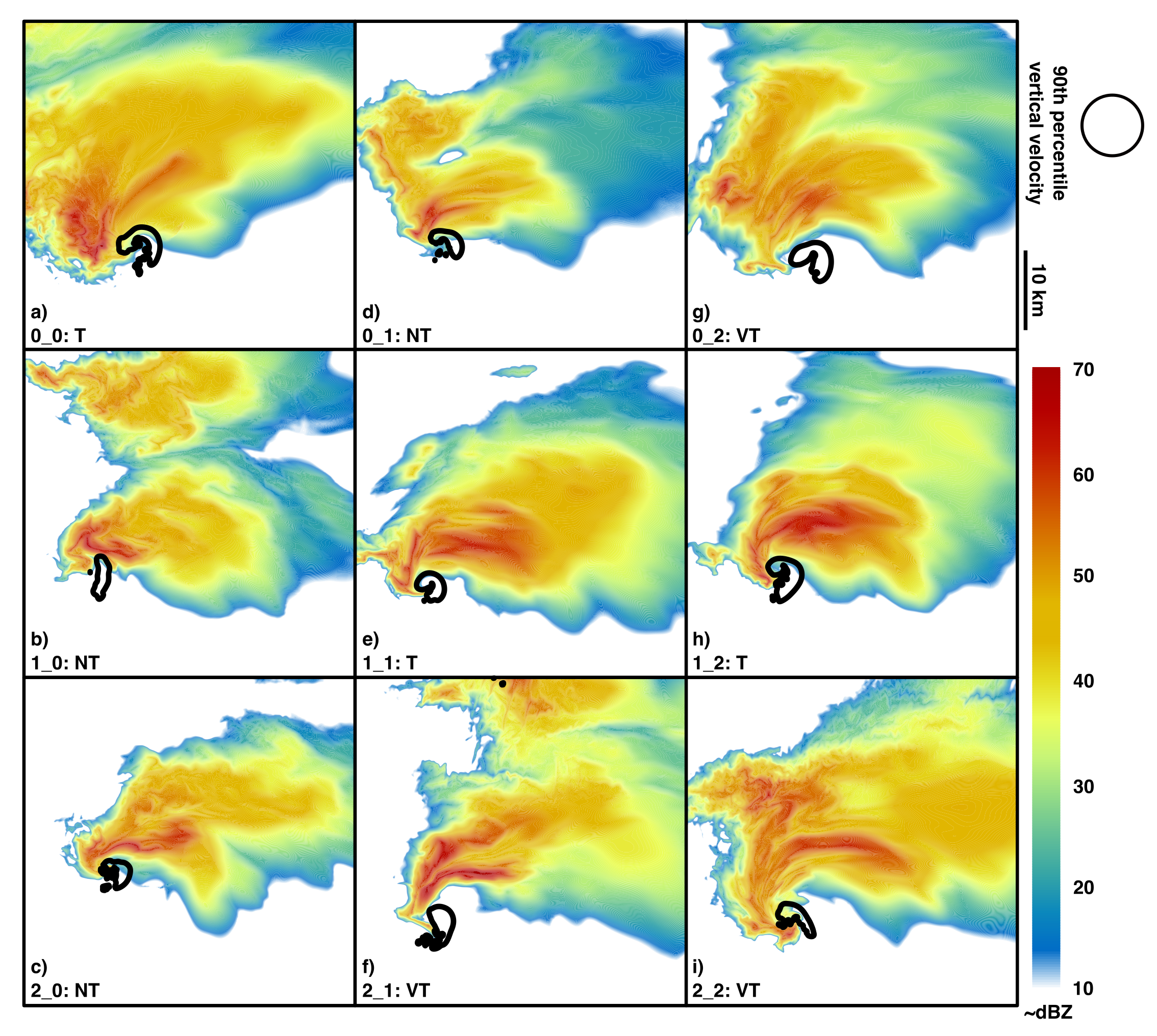
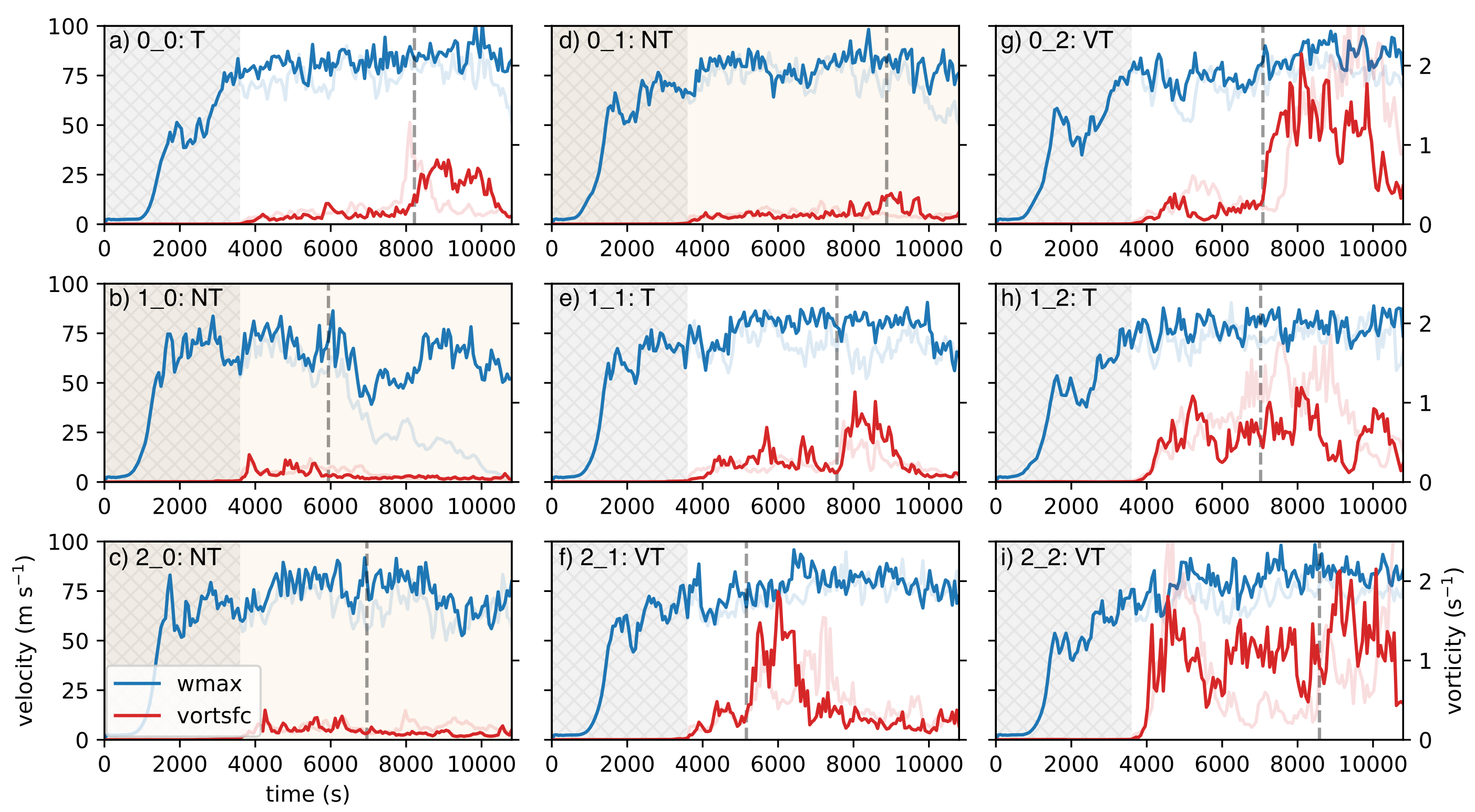
By happenstance, the nine simulations can be evenly separated into three groups of three, nontornadic (1_0, 2_0, 0_1), tornadic (0_0, 1_1, 1_2), and violently tornadic (2_1, 0_2, 2_2). The tornadic simulations are found further to right of the SOM (Fig. 1) following trends in the increasing magnitude of SRH500. The three nontornadic simulations all had SRH500 less than 100 m2 s-2, although this threshold did not preclude the 0_0 simulation from becoming tornadic (indicating that maybe some amount of storm-generated augmentation was more prominently present in this simulation). Qualitatively, the nontornadic supercells display muted trends in surface vertical vorticity (Fig. 4b-d) and never meet the threshold of a deep, long-lasting vortex underneath the main low-level mesocyclone, whereas the tornadic simulations experience abrupt jumps in the maximum surface vertical vorticity (Fig. 4a,e-i). The six tornadic simulations can be further delineated by their max . Vortex intensity increases from 0.2 in three of the simulations (0_0, 1_1, 1_2) to in the violently tornadic ones (2_1, 0_2, 2_2; Table 1). Some of the tornadic simulations experience multiple periods of tornadic activity. In such cases, our analysis on the origins of inflow into the supercells is performed on the low-level mesocyclone that resulted in the most intense tornado, as defined by , throughout the simulation.
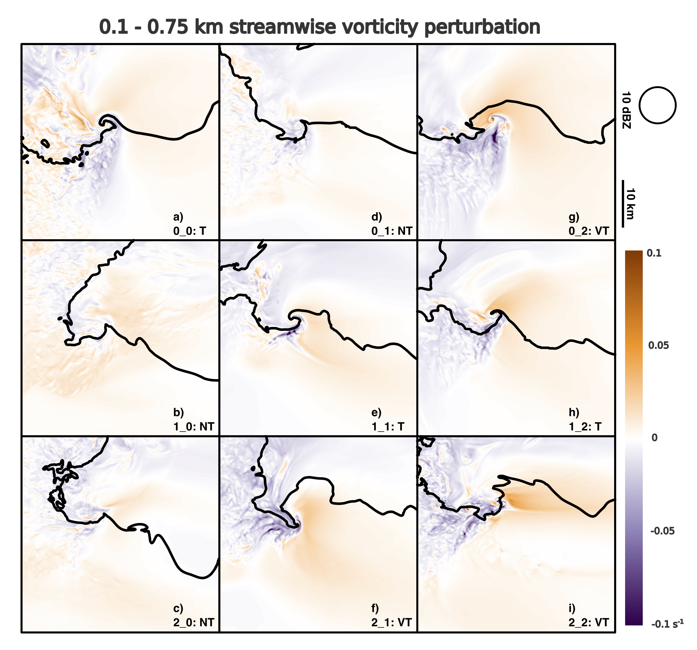
Each supercell, regardless of tornadic outcome, displays a region of enhanced streamwise vorticity relative to the base-state environment throughout the near-inflow and within the forward flank region at the key time period of tornado-genesis/failure (Fig. 5). Whether or not these features would be classified as SVCs is beyond the scope of this paper, but there is a correlation between the strength of the low-level updraft (Table 1) and larger streamwise vorticity perturbations in the inflow and forward flank regions (Fig. 5f-i). The cause of this correlation is unclear. It is possible that enhanced streamwise vorticity leads to stronger updrafts. It is also possible that stronger low-level updrafts induce greater horizontal stretching of streamwise vorticity via near-ground horizontal accelerations. The latter explanation leads to the most intense regions of streamwise vorticity within the SVC vorticity budgets analyzed by Schueth et al. (2021). Nevertheless, this question regarding the importance the enhanced regions of streamwise vorticity further motivates the subsequent analysis of the origins of inflow and vorticity within supercell low-level mesocyclones, which we explore next.
|
|
|
|
|
|
||||||||||||||
|---|---|---|---|---|---|---|---|---|---|---|---|---|---|---|---|---|---|---|---|
| 0_0 | t = 137 | 8.7 | 20.5 | 51.6 (EF2) | 0.81 | 0.21 | |||||||||||||
| 1_0 | t = 99 | 3.3 | 7.6 | nontornadic | – | – | |||||||||||||
| 2_0 | t = 116 | 6.0 | 15.1 | nontornadic | – | – | |||||||||||||
| 0_1 | t = 148 | 6.9 | 13.1 | nontornadic | – | – | |||||||||||||
| 1_1 | t = 126 | 6.9 | 21.5 | 52.8 (EF2) | 1.13 | 0.29 | |||||||||||||
| 2_1 | t = 86 | 10.1 | 27.9 | 84.7 (EF4) | 1.87 | 1.01 | |||||||||||||
| 0_2 | t = 118 | 8.4 | 29.3 | 96.6 (EF5) | 2.15 | 1.20 | |||||||||||||
| 1_2 | t = 117 | 6.6 | 30.5 | 67.9 (EF3) | 1.19 | 0.22 | |||||||||||||
| 2_2 | t = 143 | 14.6 | 41.6 | 97.2 (EF5) | 2.15 | 1.32 |
3.2 Origins of low-level mesocyclone inflow air
Supercells are largely considered to be products of the environments in which they form. The vertical distribution of quantities such as temperature, moisture, and winds, exert substantial influence over a supercell’s evolution. While previous studies have advanced our understanding of the inflow properties that favor supercells that produce tornadoes (compared to seemingly similar nontornadic supercells), questions still remain about where, both horizontally and vertically, supercells of varying intensity source most of their inflow air into the low-level updraft and mesocyclone. This in turn may shed light on the comparative importance of environmental air versus air that is modified within the storm.
3.2.1 Tracers
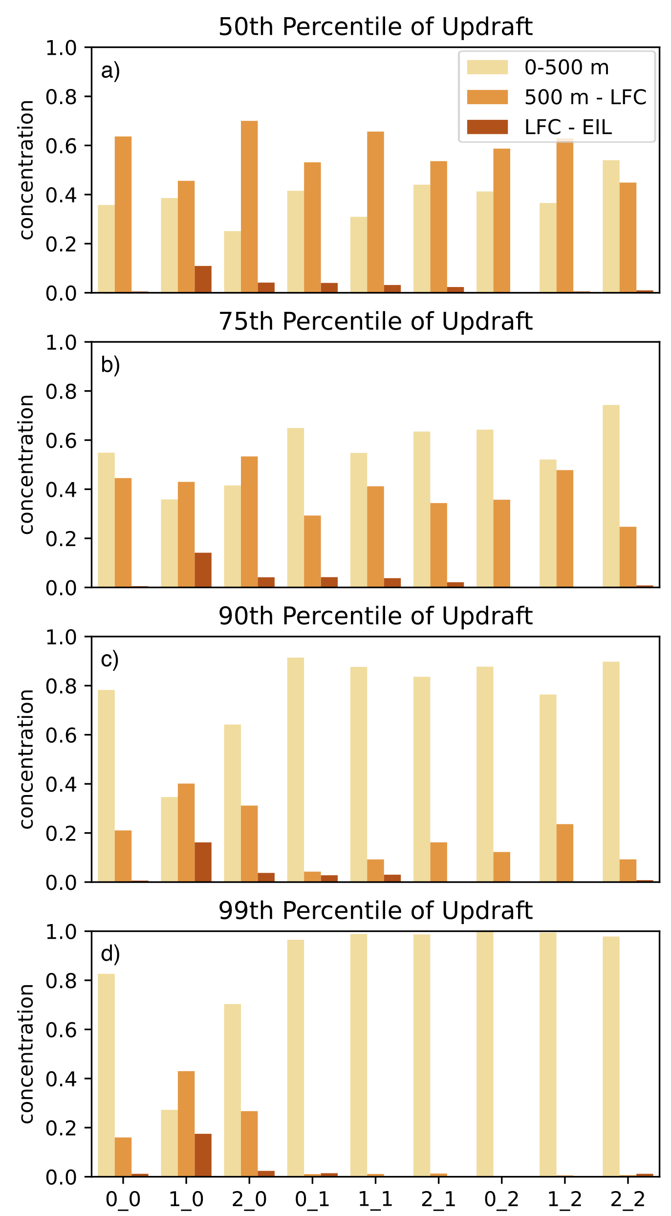
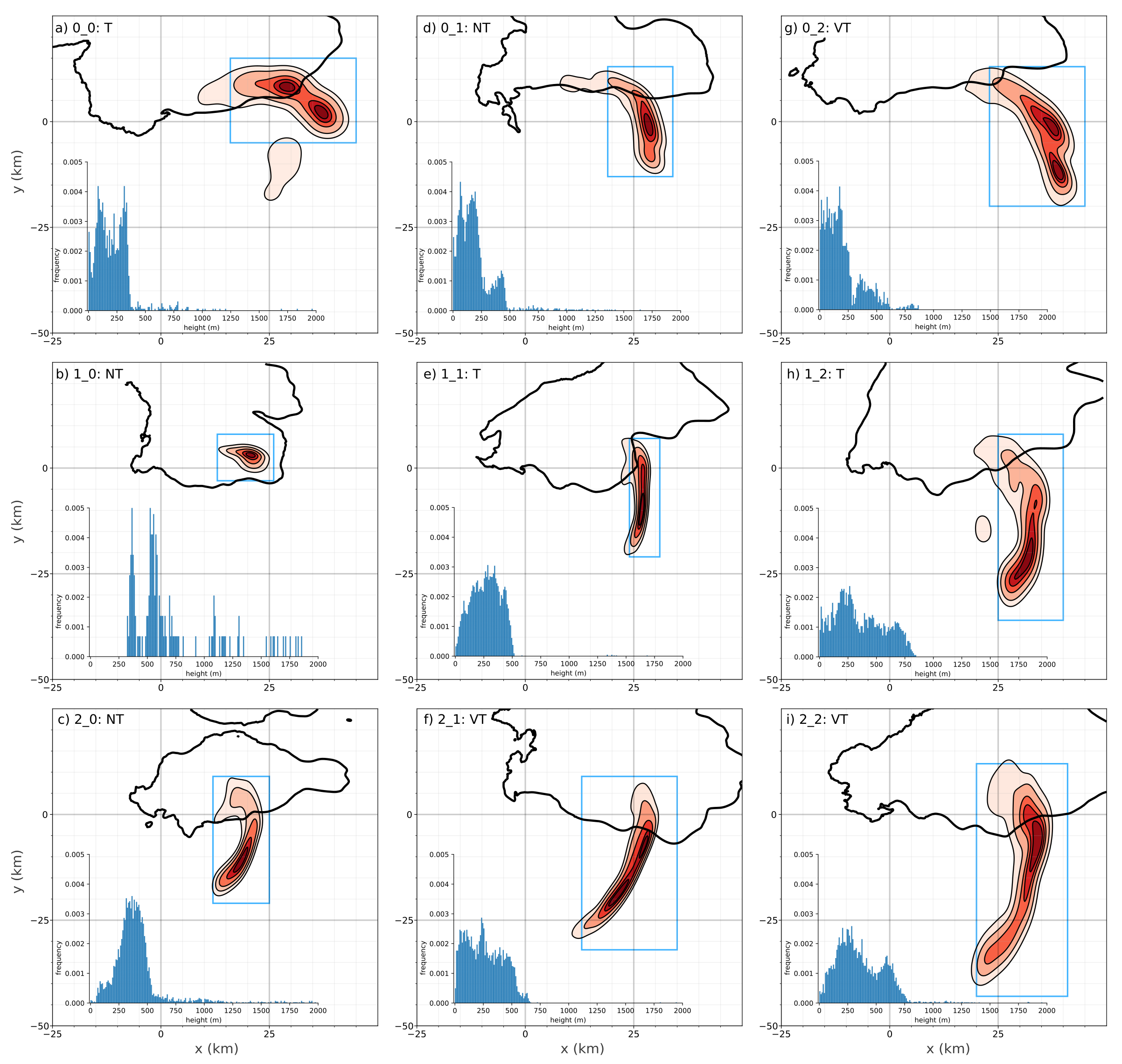
To first broadly understand the height from which the low-level updraft draws most of its inflow, we use tracers initialized within three layers: 0 – 500 m AGL, 500 m – LFC, and the LFC – EIL. Within a 10 km diameter of the 1 km AGL low-level mesocyclone centroid, the progressively stronger parts of the low-level updraft are increasingly made up of air originating from below 500 m during a five minute composite period ( to ) relative to the key time period of tornado-genesis/failure (Fig. 6). For the 50th percentile of vertical velocity ( 2 m s-1) and above, the supercell’s low-level updraft is a mixture of air from below the LFC, with the largest proportion of air generally originating between 500 m AGL and the LFC (Fig. 6a). As the updraft threshold is increased (50th 75th 90th 99th percentile) from gently rising air to the fastest rising air (and thus the largest ), the concentration of air from the near-ground layer increases substantially across seven out of the nine simulations. At and above the 99th percentile of updraft values within the low-level mesocyclone, most simulations contain essentially pure, undiluted near-surface air, with a concentration of tracer mass mixing ratio of nearly 1 (Fig. 6d), especially in the tornadic simulations. While tracers cannot indicate whether this near-ground air is coming directly from the environment or has passed through the forward flank baroclinic zone, concentration values approaching unity within the core of the low-level updraft are indicative of air that is largely unmodified by the storm’s outflow since re-ingested forward flank air parcels would tend to experience dilution from mixing. Simulations 1_0 and 2_0 (both nontornadic and having the lowest environmental SRH500 values) are noticeable outliers to this trend, although even in 2_0, at least 60% of the low-level updraft air is being fed by the near-ground layer. Compared to other tornadic simulations, the 0_0 supercell has marginally less (15–20%) near-ground air within the low-level mesocyclone (an indication that this low-level mesocyclone, in a lower SRH500 environment, perhaps is supplemented by other sources of air).
The explanation for the importance of the near-ground layer in the low-level mesocyclone relates to the ascent angle () of the storm-relative wind into an updraft. As inflow air approaches the storm and enters the footprint of the updraft, vertical tilting of horizontal vorticity occurs. From Peters et al. (2023), the tilting of horizontal vorticity in a perfectly streamwise environment can be expressed as:
| (2) |
where is streamwise vorticity, is the vertical velocity of the updraft, and is the storm-relative wind [Davies-Jones (2022) presents a similar equation]. Although the wind profiles in Figure 1 are not perfectly streamwise, Eq. 2 represents a good first order approximation of the tilting of horizontal vorticity into a mature, right-moving supercell’s updraft.
The simplest interpretation of Eq. 2 is that the tilting of is related to the slope of trajectories entering an updraft (i.e., “rise over run” or ). The efficiency of the tilting of environmental streamwise vorticity into the vertical is modulated by the balance between vertical and horizontal motion (also discussed in Davies-Jones, 1984; Droegemeier et al., 1993). Peters et al. (2023) found that varies with updraft width and storm-relative flow, but the median for parcels bound for the low-level mesocyclone across a spectrum of supercell wind profiles was approximately 10∘, averaged across all their simulations. Thus, the slope of the trajectories into low-level mesocyclones is fairly gentle. Only parcels originating from the near-ground layer are likely to have fully converted into by 1 km AGL. Thus, as suggested by Markowski et al. (2012b), large near-ground streamwise vorticity establishes the base of the low-level mesocyclone as close to the surface as possible given typical ascent angles, inducing a “dynamical feedback” process of pressure falls and upward directed perturbation pressure gradient accelerations (Goldacker and Parker, 2021) needed for lifting and stretching negatively buoyant, circulation-rich air within the supercell’s outflow.
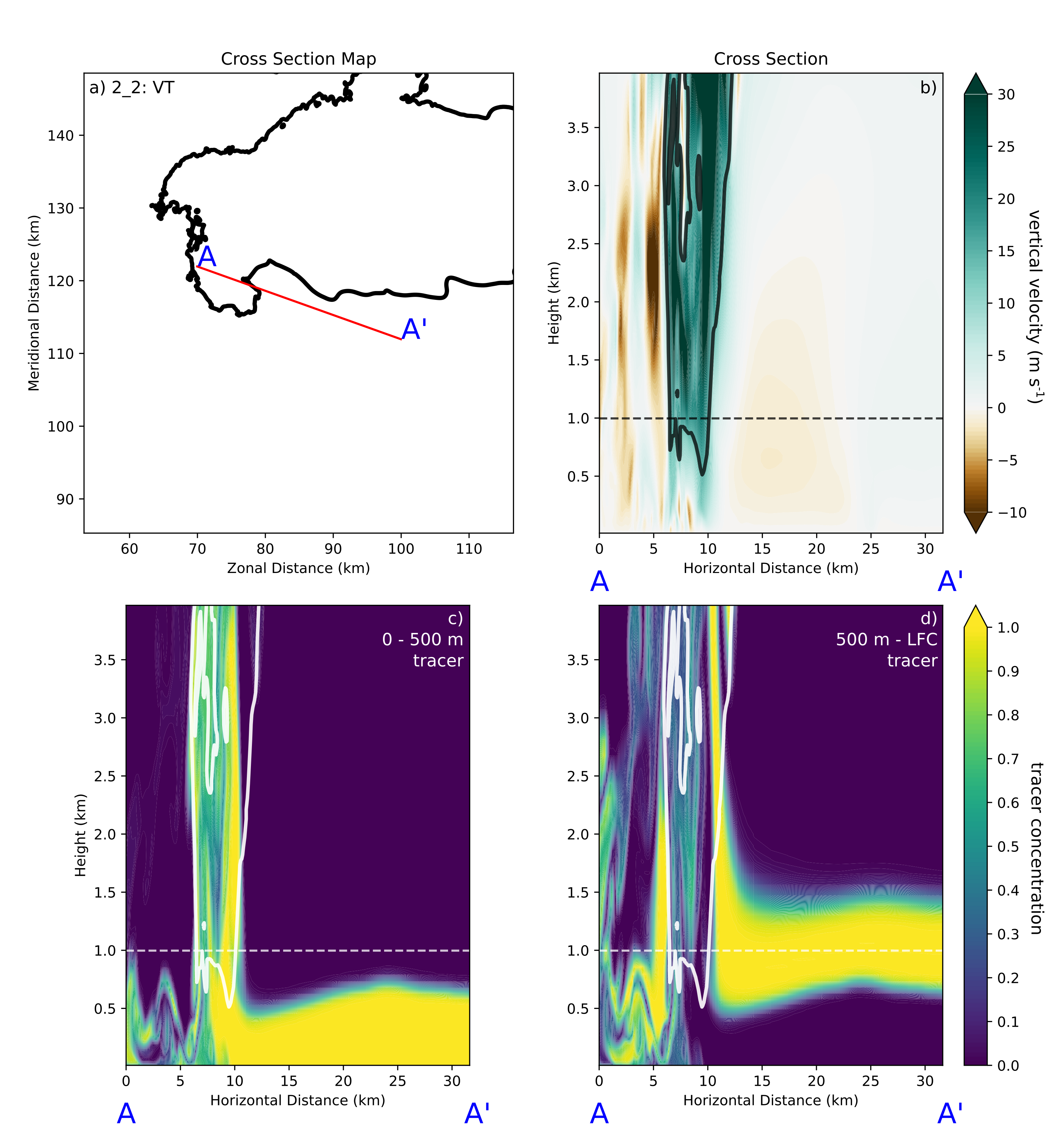
In the current simulations, cross-sections through the low-level updraft display similar trends in ascent angles and tracer concentrations within the supercell’s updraft at varying altitudes. For the 2_2 supercell (Fig. 7), even prior to tornadogenesis, an intense core of vertical velocities greater than 15 m s-1 extends down to 500 m AGL (Fig. 7b), with the maximum 1 km updraft exceeding 40 m s-1 (Table 1). Within the updraft from 500 m – 1 km AGL, the concentration of air from the near-ground layer is essentially one (Fig. 7c). In fact, this is generally the case within the core of the updraft up to 2 km AGL. At this point, a much larger concentration of air from 500 m to the LFC is present (Fig. 7d). Both Nowotarski et al. (2020, their Fig. 5) and Lasher-Trapp et al. (2021, their Fig. 14) show examples of this gentle ascent layer, where air in the upper part of the inflow layer (i.e., 500 m – 2 km AGL) does not contribute to the core of the updraft until much farther aloft (i.e., 2 – 4 km AGL). Below 2 km AGL, what little air that is present from above 500 m is predominately found along the downshear (i.e., the eastern) edge of updraft (Fig. 7d).
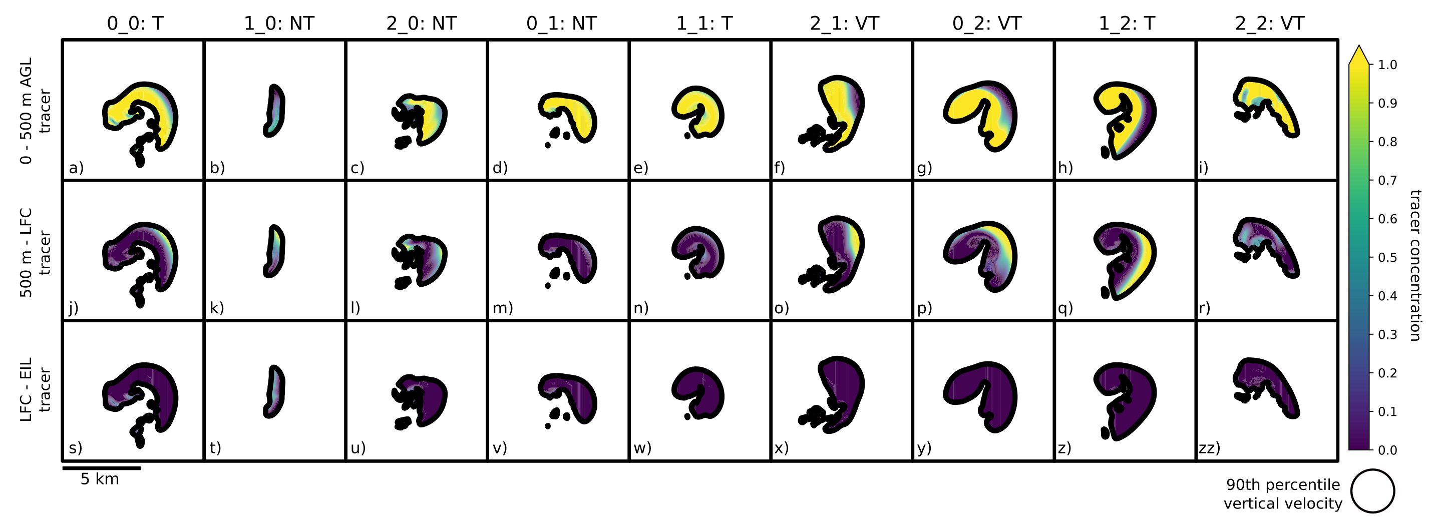
Across eight of the nine simulations herein (with the transient 1_0 supercell again being the outlier), for updrafts defined by the 90th percentile of vertical velocity and above, the highest concentration of air is definitively from the 0 – 500 m layer (Fig. 8a,c-i). Where air above this layer contributes most substantially is along the eastern, downshear flank of the updraft (Fig. 8j,l-q). This is consistent with this air stream not yet being fully titled into the vertical (Eq. 2) and residing along the edge of the updraft footprint. Air originating from above the LFC is not found with any consistency within the core of the supercells’ updraft at any height within the troposphere (not shown), and accordingly is virtually non-existent in the low-level mesocyclone (Fig. 8s-zz). Although this is likely not surprising given the altitude of the LFC ( 1.7 km), there is a historical precedence in tornado forecasting of integrating SRH over depths much greater than the LFC [e.g., 0 – 3 km AGL SRH in Rasmussen and Blanchard (1998) and SRH in the EIL (ESRH) in Thompson et al. (2007)]. While shallower layers of SRH have the highest correlation with low-level updraft and mesocyclone intensity (compared to the mid-level mesocyclone; Peters et al., 2023), the height at which the wind profile no longer affects tornado potential is currently unknown. Any statistically significant differences in wind profiles between nontornadic and tornadic supercells above the lower troposphere could be due to direct influences of the mid-level updraft/mesocyclone at lower altitudes (such as lowering the base of the mid-level mesocyclone, as suggested by Markowski et al., 2012b) or indirect influences on the storm (such as modifying the deviant rightward storm motion or altering the downstream distribution of hydrometeors relative to the updraft, as suggested by Coniglio and Parker, 2020; Coniglio and Jewell, 2022). However, in the simulations presented herein, air above the LFC does not appear to contribute to the low-level mesocyclone and associated footprint of dynamic lifting.
3.2.2 Backward trajectories
Next we turn to backward trajectories initialized within the most intense upward-moving, cyclonically rotating air in the low-level mesocyclone. While the three layers of tracers show that the low-level mesocyclone is predominately made up of near-ground air, tracers alone cannot show the inflow origins of air bound for the low-level mesocyclone (e.g., the undisturbed, ambient environment versus the forward-flank baroclinic zone). To address this, we initialized backward trajectories within the 90th percentile of vertical velocity at 1 km AGL in each simulation, as this area has the highest potential for stretching of subtornadic surface vortices into tornadoes.
|
|
|||||
| 0_0 | 190.6 | 336.5 | ||||
| 1_0 | 562.4 | 1325.3 | ||||
| 2_0 | 368.7 | 528.7 | ||||
| 0_1 | 161.9 | 403.8 | ||||
| 1_1 | 274.0 | 436.6 | ||||
| 2_1 | 245.1 | 487.4 | ||||
| 0_2 | 161.4 | 435.1 | ||||
| 1_2 | 310.0 | 681.5 | ||||
| 2_2 | 321.0 | 630.9 |
During a five minute period prior to tornado-genesis/failure ( to ), the origin height of inflow air into the mesocyclone is highly consistent across eight of the nine supercells. Similar to the tracer analysis, backward trajectories bound for the low-level mesocyclone originate very close to the ground (Table 2). The distributions of the origin height of trajectories shown in the insets of Figure 9 are generally below 500 m (excluding 1_0). The median origin height for the eight main supercells is less than 400 m AGL and 90% of the parcels in each simulation come from below 700 m AGL (Table 2). Only a few trajectories across the matrix of supercells represent “recycled air”, or air with a history of descent from farther aloft555The exact path of “recycled” low-level mesocyclone trajectories should be treated with caution since the likelihood of errors in the backward trajectory integration is higher for such a flow regime. Regardless, the overwhelming proportion of trajectories that rise into the low-level mesocyclone from the undisturbed inflow compared to the “recycled air” is still qualitatively informative. (Fig. 10). Many of the simulations have median parcel heights less than 300 m (Table 2). The very low altitude of parcels that contribute to the strongest vertical motion within the mesocyclone likely explains the comparative forecast skill of environmental streamwise horizontal vorticity and thus environmental SRH in progressively shallower layers (e.g., as shallow as 0 – 250 m AGL in Coffer et al., 2020).
Compared to the vertical extent of the inflow, the horizontal extent of air bound for the low-level mesocyclones across the simulations generally originates from south and east of the low-level updraft (Figs. 9,10), consistent with the orientation of the near-ground hodographs in Figure 3. The trajectory fields in the simulations with higher SRH have a noticeably more expansive inflow region, especially towards the southeast (Fig. 9e-i). The highest density of parcel origins in most of the simulations (Fig. 9d-i) is from well outside of the precipitation field. The paths of these trajectories, coming from the undisturbed, far-field environment into the low-level mesocyclone, appear to traverse the forward flank only minimally (or not at all in some instances, e.g., Fig. 10d,g). Especially for the tornadic supercells, the parcel origins are mostly from the far-field, toward the southeast (Fig. 9e-f-i), with one exception (0_0). In 0_0, the initial locations are primarily due east of the low-level mesocyclone (Fig. 9a) and flow parallel to the forward flank (Fig. 10a), consistent with the orientation of the storm-relative wind in the 0_0 hodograph (Fig. 1a). The prevalence of parcels originating from the undisturbed inflow environment is consistent across multiple possible definitions of a “low-level mesocyclone”. Coherent areas of large, positive circulation at 1 km AGL display very similar trajectory origins and statistics (see Supplemental Figs. 1-3), due to a high degree of correlation between the areas of large circulation and large vertical velocity (not shown).
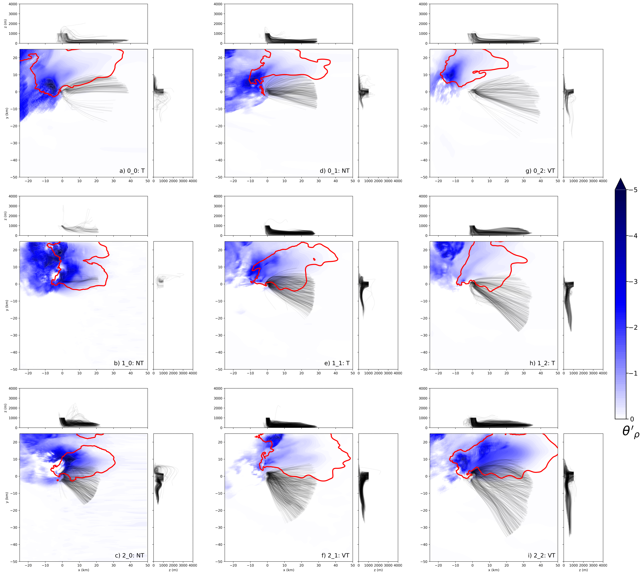
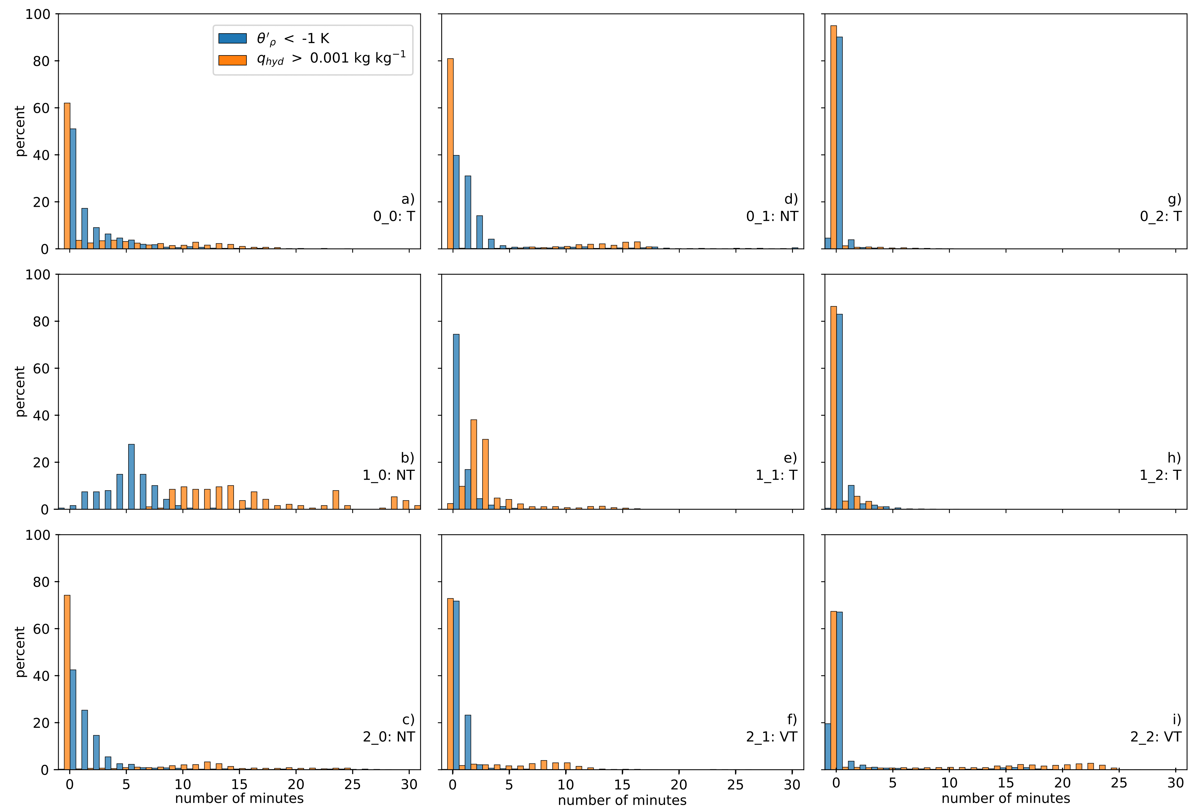
At least 65% of parcels bound for the low-level mesocyclone in the eight main supercells spend less than 5 minutes in areas influenced by the storm’s hydrometeor and negative buoyancy fields (Fig. 11), based on the accumulated time within regions characterized by kg kg-1 and K. These two, admittedly arbitrary, thresholds only provide an estimate of the time the backward trajectories spent within ’storm outflow’, not the potential for baroclinic streamwise vorticity generation (which is explored more thoroughly using the material stencils in the subsequent subsection). In the instances characterized by the weakest forward flank cold pools (Fig. 10f,g,h), this percentage is greater than 90%. For the small percentage of parcels that do interact with baroclinic gradients associated with the forward flank, the experienced deficits in density potential temperature rarely exceed -2 to -3 K, and are generally closer to -1 K (Fig. 10). Cold pool deficits are often even weaker 30 minutes prior to tornado-genesis/failure, when the trajectories were initialized, than Figure 10 would suggest (not shown). In that respect, the density potential temperature fields in the present simulations resemble those of the observed tornadic supercells in Shabbott and Markowski (2006). As a result of the short residence time within the storms’ forward flanks, weak deficits in potential temperature, and fast storm-relative winds accelerating towards the supercell, the mean low-level mesocyclone trajectory in the eight main supercells experiences a rather small change in streamwise horizontal vorticity along its inflow path [estimated using Eq. 1 from Shabbott and Markowski (2006)] . This is more precisely quantified with the material stencils in the following section.
In summary, inflow air into the low-level mesocyclone originates very close to the ground and overwhelmingly from the undisturbed, far-field environment (toward the southeast). Most parcels bound for the low-level mesocyclone experience minimal effects from the storm’s precipitation field. Both of these results would be expected to have a direct effect on the importance of environmental versus storm-generated vorticity contributions to the low-level mesocyclone. We explore this topic directly next.
3.3 Contributions of environmental vs. storm-generated vorticity to the low-level mesocyclone
Through both tracers and backward trajectories, we have shown thus far that the air comprising the most intense upward-moving, cyclonically rotating air in the low-level mesocyclone originates from the near-ground layer (500 m AGL) and predominately from the undisturbed inflow environment, with the highest density of parcels appearing to have very little residence time within the region of precipitation and negative buoyancy associated with the forward-flank region. On the face of it, these two factors would seemingly implicate the near-ground environmental horizontal streamwise vorticity as the dominant contributor to the overall rotation of the low-level mesocyclone, not the storm-generated streamwise vorticity classically associated with low-level mesocyclone-genesis. To quantitatively evaluate this interpretation, we track forward trajectories bound for the low-level mesocyclone and assess their associated vorticity via stencils of nearby adjacent parcels following the technique described by Dahl et al. (2014). As described in Section 2, forward trajectories were seeded within model restart files upstream of the low-level mesocyclone within a unique horizontal bounding box for each simulation (the blue boxes in Fig. 9) encompassing at least 75% of the low-level mesocyclone inflow area based on the origins of the backward trajectories. The seeding of the forward trajectories is meant to represent a majority of the inflow air; computational limitations prevent an exhaustive sample of all possible inflow air.
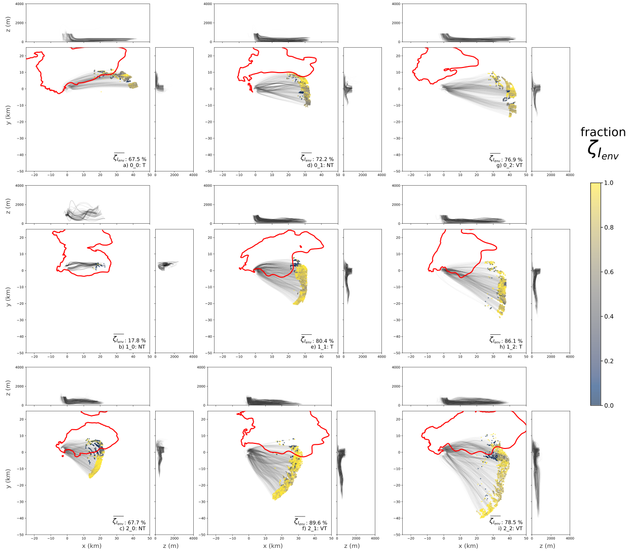
The forward trajectory parcels that meet the vertical velocity and vertical vorticity thresholds of the low-level mesocyclone [vertical velocities greater or equal to the 90th percentile at 1 km AGL (Table 1) and at least 0.01 s-1 of vertical vorticity (within 10 m of 1 km AGL)]666An overwhelmingly majority of the forward trajectories released within the inflow region would have qualified as low-level mesocyclone parcels if the parcel output frequency was decreased and/or the depth of the vertical layer surrounding 1 km AGL was increased. These choices simply acted to filter parcels to a reasonable number for analysis given storage and computational constraints. have similar paths into the low-level mesocyclone and originate from similar locations as the backward trajectories in the previous section (Fig. 12). This provides some quality assurance, which is welcome in light of documented differences in accuracy between forward and backward trajectory techniques (Dahl et al., 2012). Because the forward trajectories were not seeded at the exact terminal locations of the backward trajectories (rather, they were initialized over an isotropic grid covering most of the inflow region), it is not possible to directly compare the two sets of trajectories (as-in Dahl et al., 2012, Gowan et al. 2021); however, many of the details, including the shape, width, depth, and proportion of undisturbed, far-field environment parcels to forward flank parcels, are extremely similar (Figs. 10, 12).
Each seven-parcel stencil tracks and (as described in Section 2) via the deformation and stretching of the initial (or “imported”) vorticity vector over time, while (and the rearrangement of ) is computed as a residual. In eight of the nine simulations (except 1_0), is far and away the dominant contributor to the low-level mesocyclone vertical vorticity777The percentage of and to the total was calculated via both a simple ratio as well as a weighted average by the magnitude of . Percentages from either method resulted in very similar results presented in Figs. 12,13; however, in general, the contribution from using the weighted average was approximately 3-5% higher across the simulations, implying parcels that develop additional vorticity from storm-generated sources contribute slightly more to strongest rotation of the low-level mesocyclone. (; Fig. 13a). Only in simulation 1_0, the weakest and most transient supercell, is the dominant component of . This is not entirely unexpected considering the entire inflow region of the 1_0 supercell’s low-level mesocyclone originates within precipitation of the forward flank (Figs. 9b, 10b, 12b). For the other eight main simulations, contributes between 65% and 90% of the total indicating that the environmentally-derived vorticity comprises a much larger percentage of the mesocyclone’s vertical vorticity than the storm-generated vorticity (Fig. 13a). The dominant contribution of to the total is consistent across multiple possible definitions of a “low-level mesocyclone”, including for lower altitudes than 1 km AGL (specifically at 750 and 500 m AGL; see Supplemental Fig. 4) and for a coherent area of positive circulation (regardless of vertical velocity and vertical vorticity values; see Supplemental Figs. 1-3,5).
While is generally quite high for all these eight simulations, there is a trend for the tornadic supercells towards the right of Figure 13a, starting with 1_1, to have a higher percentage of than the nontornadic supercells. These tornadic simulations also have the most favorable lower tropospheric base-state hodographs and the highest values of SRH500. The exception to that trend, simulation 0_0, has 20% lower contribution from than the other tornadic supercells (Fig. 13a). Not only does the 0_0 supercell have a base-state SRH500 of 67 (well below the median tornadic SRH500 value from Coffer et al., 2019), but also has the lowest concentration of near-ground tracer among the tornadic low-level mesocyclones (Fig. 6) and highest proportion of parcels that flow into the mesocyclone directly parallel to the forward flank baroclinic gradient (Fig. 10). In total, this potentially suggests the 0_0 supercell required additional augmentation from within storm baroclinic generation of streamwise vorticity to establish a low-level mesocyclone capable of producing a tornado. Fully fleshing out this hypothesis would require an ensemble of simulations and more additional analysis, which is beyond the scope of this study and will be expanded upon in future work.
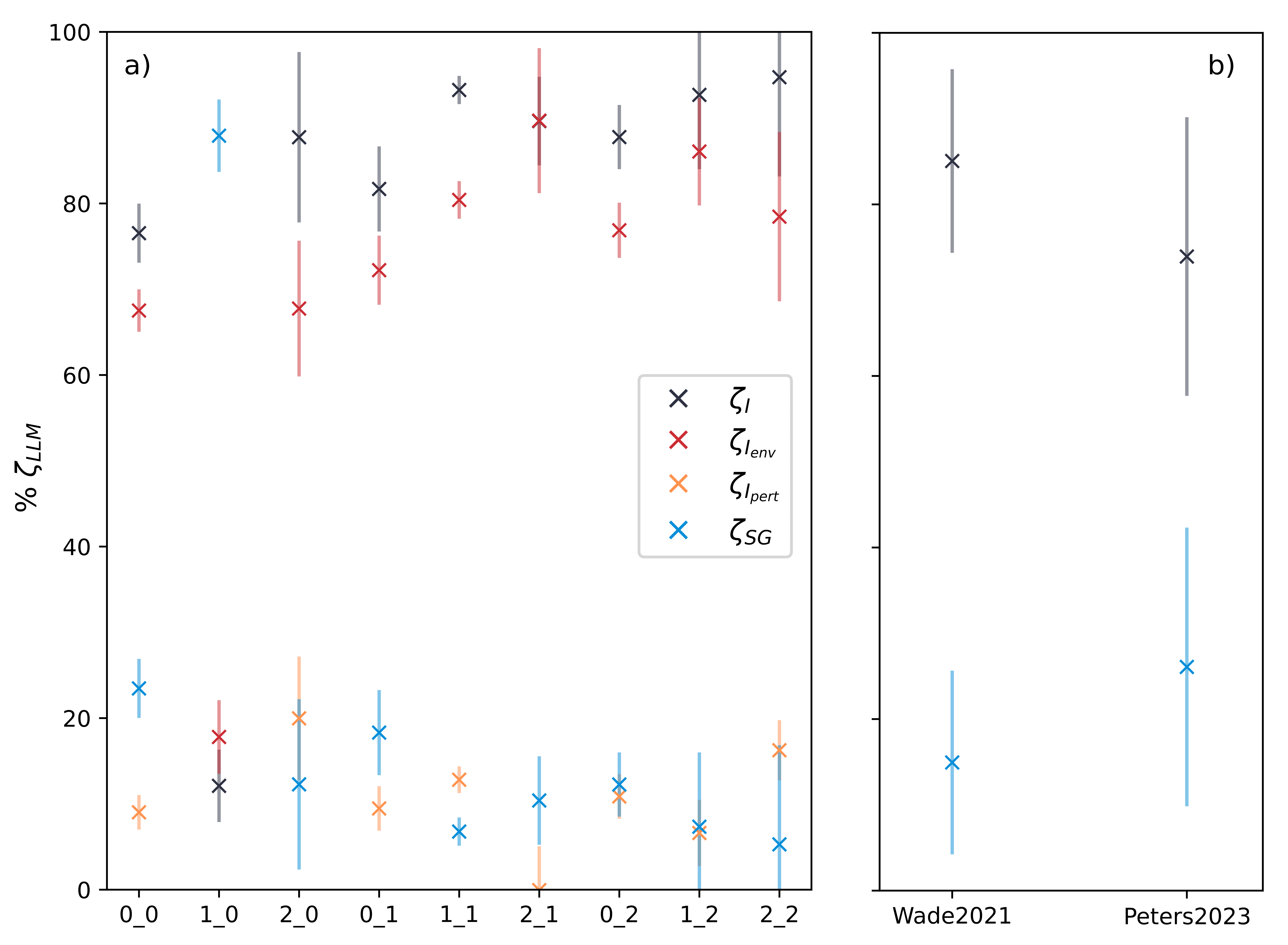
The next largest contributor to (either or ) varies between the individual simulations but is generally less than 20%. There is no discernible trend for the nontornadic or tornadic supercell simulations to have more or less than . As a reminder, because we cannot say whether the represents prior reorientation or stretching of base-state vorticity versus prior baroclinic (or frictional) generation, it is treated separately. Even if we generously assume is entirely attributed to storm-generated effects, their combined contribution would still be less than 35% of the total for the eight main storms.
While the bulk percentages of compared to paint a clear picture that most of the low-level mesocyclone rotation is from the environmental vorticity, examining individual parcels and their ratio of to highlights source regions from which generation from the storm is more prominent, such as the forward flank. There is a trend in some (but not all) of the supercells to have lower percentage of within parcels that originate closer to the hydrometeor field and forward flank (Fig. 12c,e,i). Those three simulations (2_0, 1_1, 2_2) also represent simulations where the backward trajectories cross through larger density potential temperature gradients (Fig. 10c,e,i) and have a higher frequency of parcels that spend 5 – 25 minutes of accumulated time within the hydrometeor and negative buoyancy fields (Fig. 11c,e,i). Specifically looking at simulation 2_2 (Fig. 12i) as an example, many of the parcels with the lowest percentage of (and thus highest ; located at approximately x=30, y=-5 in Fig. 12i) traverse west-northwestward into forward flank (and larger negative buoyancy gradients; Fig. 10i), before turning back towards the updraft and eventually rising into the low-level mesocyclone. Due to their path through the storm, and exposure to horizontal baroclinity, these isolated parcels likely correspond to the classical conceptual model of forward flank air being re-ingested into the low-level updraft and wall cloud (i.e., Atkins et al., 2014, see their Fig. 5).
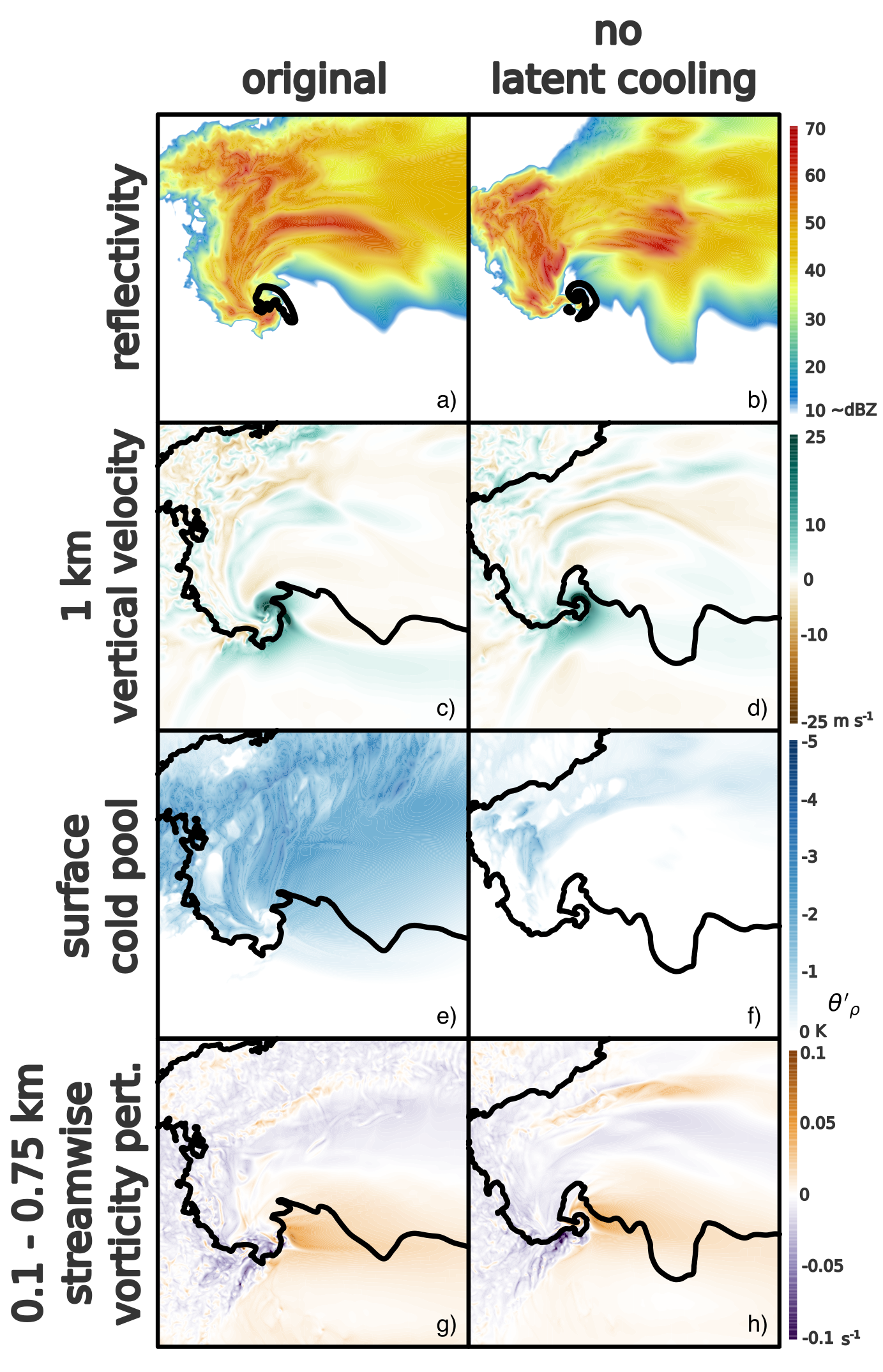
As a final test of the apparent unimportance of baroclinic generation within the forward flank to the low-level mesocyclone, the 2_2 simulation was rerun without evaporation, melting, or sublimation (i.e., no latent cooling) for the 30 minutes prior to the key time period of tornadogenesis. Despite having almost no remaining cold pool, a similarly intense low-level mesocyclone occurs in the cooling-free experiment ( ¿ 40 m s-1; Fig. 14c,d). And, an almost-identical region of enhanced streamwise vorticity within the near-inflow region also persists when microphysical cooling is turned off ( ¿ 40 m s-1; Fig. 14g,h). Although we cannot rule out the possibility of some prior memory of a baroclinic forcing and/or a convergent boundary within the forward-flank, there is essentially no lasting negative buoyancy present within the forward flank (Fig. 14f; besides the minimal contribution from hydrometer drag). Thus, the SVC-like feature present must be due to horizontal stretching of the ambient, environmental vorticity (contained within the term in the realm of material stencils) in response to the inflow low associated with the updraft. Schueth et al. (2021) also found that the maximum vorticity in their simulated SVC was almost solely driven by horizontal stretching. This sensitivity test underscores the importance of the environmental vorticity since a similarly-intense low-level mesocyclone occurs in the absence of baroclinic generation.
3.3.1 Low-level mesocyclone vorticity sources in supplemental simulations
On one hand, because of the documented forecast skill of near-ground environmental SRH in separating nontornadic from significantly tornadic supercell environments, it seems entirely logical that the environmental vorticity would exert a substantial influence on the total vertical vorticity of the low-level mesocyclone. On the other hand, because the low-level mesocyclone has often been attributed to baroclinically-generated streamwise horizontal vorticity within the storm (as discussed in the introduction), the degree to which dominates, and consistency among the simulations, is somewhat surprising. To supplement the results from the simulations presented herein, we also present previously unpublished material stencil analyses from two existing supercell studies in the literature, Wade and Parker (2021) and Peters et al. (2023).
These studies complement our simulations by virtue of their different thermodynamic and kinematic environmental profiles. Wade and Parker (2021) focused on three high-shear, low-CAPE (HSLC) environments from a VORTEX-SE case in Alabama on 31 March 2016 as well as a companion high-shear, high-CAPE environment from the 3 April 1974 “Super Outbreak” (see their Fig. 6 for Skew - and hodograph diagrams). Peters et al. (2023) presented a large number of supercell simulations with “L” and “C” shaped hodographs (see their Figs. 1-3 for Skew - and hodograph diagrams), independently varying the streamwise vorticity and storm-relative flow to disentangle their influence on low-level mesocyclone characteristic. Each simulation in Peters et al. (2023) used a constant thermodynamic environment based on the tornadic VORTEX2 composite environment from Parker (2014). The reader is referred to these papers for more details about their simulations. The material stencil analysis was conducted independently amongst the three studies, with varying thresholds of vertical velocity/vertical vorticity and criteria for when/where forward trajectories were seeded. Of note, these studies calculated and only; no attempt was made to distinguish from . The chief similarity between all three studies is that parcels were filtered to highlight those entering the low-level mesocyclone at 1 km AGL. We believe the modest differences in analysis techniques increase confidence that the results presented in the previous subsection are not unique to our specific methodological choices.
Similar to the eight main supercell simulations in the present study, the low-level mesocyclones of both Wade and Parker (2021) and Peters et al. (2023) primarily derive vertical vorticity from the environment rather than storm itself (Fig. 13b). In the Wade and Parker (2021) storms, the low-level mesocyclone is almost entirely environmentally driven for the parcel groups in the high-CAPE storm and low-CAPE 1 and 3 ( 85%). Even in their low-CAPE 2 supercell, which in general presented more analysis challenges than the other three supercells [see Wade (2020) for more details], the initial environmental component of the low-level mesocyclone is greater than 65%. Given the differences in storm structures and cold pools amongst the high-CAPE and low-CAPE storms (Wade and Parker, 2021), it is remarkable how consistently little the storm-generated term contributes to the low-level mesocyclone (Fig. 13b, Supplemental Fig. 6). For the Peters et al. (2023) supercells, the storm-generated component comprised less than 35% of the total on trajectories in most simulations (Fig. 13b), only exceeding this percentage in the storms with the weakest mesocyclones. Regardless of the differing combinations of storm-relative flow and streamwise vorticity, the environmental contribution was generally greater than 65%888None of the low-level mesocyclone/updraft attributes systemically evaluated in Peters et al. (2023), such as updraft and mesocyclone radius, net updraft circulation and rotational velocity, as well as average updraft vertical vorticity and helicity density, displayed any meaningful correlation with the fraction of to (Supplemental Fig. 7).. In total, these results further demonstrate that environmentally-derived vorticity comprises a much larger percentage of the low-level mesocyclone than storm-generated vorticity in persistent, mature supercells.
4 Conclusions and discussion
In this article, we sought to address where inflow air bound for the low-level mesocyclone originates from and whether the origins of such air could address the dynamical role of near-ground streamwise vorticity present in the ambient environment versus what is generated in-situ within the forward flank of a supercell. The streamwise vorticity present within the environment, and the augmentation of the vorticity by the storm, can potentially modulate the intensity the low-level mesocyclone and ultimately determine whether a supercell fails or succeeds at producing a tornado. Using a matrix of nine supercell simulations, initialized with a spectrum of near-ground wind profiles observed in nature, we found the following:
-
•
The air that comprises the core of the mesocyclone at 1 km, where the greatest potential for vertical stretching exists, originates almost exclusively from very close to the ground, often in the lowest 200 - 400 m AGL. Air originating above 500 m AGL does not tend to contribute to the main updraft until farther aloft.
-
•
Air bound for the low-level mesocyclone primarily originates from the undisturbed, ambient environment, rather than from along the forward flank. In both the nontornadic and tornadic supercells, 60 to 90% of the inflow air into the low-level mesocyclone has little to no residence time within regions characterized by negative buoyancy and hydrometeors in the forward flank.
-
•
The dominant contributor to vertical vorticity within the low-level mesocyclone is from the environmental horizontal vorticity, with storm-generated providing very little augmentation to the low-level mesocyclone. As much as 90% of the low-level mesocyclone vertical vorticity can be solely attributed to the base-state environment. For the few parcels that do traverse baroclinic gradients within the storm, the augmentation to the low-level mesocyclone from storm-generated vorticity is higher.
We were motivated to understand why near-ground environmental streamwise vorticity is such a highly skillful tornado forecast parameter given the long history linking the low-level mesocyclone intensity to within-storm baroclinic generation of horizontal vorticity (e.g., Klemp and Rotunno, 1983; Rotunno and Klemp, 1985). Low-level mesocyclone air in our simulated supercells comes from the ambient environment. Thus, low-level mesocyclone does not require much augmentation from the development of additional horizontal vorticity in the forward flank. The ingestion of forward flank parcels may instead be a symptom of an intensifying low-level mesocyclone (driven by environmental horizontal vorticity). After all, in order for rain-cooled air to be re-ingested by the storm, substantial dynamic lifting must be present to force negatively (or at least neutrally) buoyant forward flank outflow parcels upwards.
Perhaps some of the apparent prior ambiguity within the past literature can simply be attributed to differences in nomenclature between studies (or lower vertical resolution). Many of the earlier references to ’low-level mesocyclones’ within the literature discussed rotation approximately within the lowest 250 m AGL (e.g., Rotunno and Klemp, 1985; Brooks et al., 1993, 1994; Wicker and Wilhelmson, 1995; Gilmore and Wicker, 1998; Adlerman et al., 1999; Atkins et al., 1999; Ziegler et al., 2001; Beck and Weiss, 2013). Over time, with increased emphasis on the supercell’s footprint of dynamic lifting being established at relatively low altitudes, about 1 km above the ground, (e.g., Markowski and Richardson, 2014), a distinction between “near-ground rotation” and “low-level mesocyclone rotation” has developed in the literature. These earlier studies were likely quantifying the development of near-ground rotation, which has rather conclusively been attributed to baroclinic gradients and vorticity generation within downdrafts in the outflow (summarized in Fischer and Dahl, 2022b). On the other hand, the low-level mesocyclone is predominately associated with upward tilting of horizontal vorticity999Even if the forward flank contributes more to the overall rotation of the low-level mesocyclone than shown herein, these highly streamwise parcels in the lower troposphere would be tilted into the mesocyclone by an updraft, not a downdraft.. Despite the apparent evolving definition of term ’low-level mesocyclone’, there is still widespread reference to Rotunno and Klemp (1985) in recent years regarding the development of low-level mesocyclone rotation, even when clearly discussing rotation near the cloud base (e.g., Orf et al., 2017; Frank et al., 2018; Markowski, 2020; Fischer and Dahl, 2020; Flournoy et al., 2020, 2021; Murdzek et al., 2020b, a; Schueth et al., 2021; Davies-Jones, 2022; Finley et al., 2023). We encourage future research endeavours to use a unified nomenclature when discussing supercell processes in the lower troposphere, as the governing dynamics between the development of rotation near the ground ( 250 m AGL) and near cloud-base ( 1 km AGL) are very likely distinct (at least prior to tornadogenesis).
Future studies could also clarify the conceptual distinction between “low-level” and “mid-level” mesocyclones. If both are generated via the upward tilting of environmental horizontal vorticity, at what point does the lowest portion of the mid-level mesocyclone impact the rotation near cloud-base? Are mesocyclones truly bi-modal as the community has often defined them? Vertical profiles of vertical vorticity leading up to the tornadic phase of a supercell in Klemp and Rotunno (1983, their Fig. 6), as well as across the matrix of simulations presented herein (Supplemental Fig. 8), appear to substantiate the distinction of the low-level mesocyclone near cloud-base from the mid-level mesocyclone. Across all nine simulations, there is a specific local maximum in the vertical vorticity field at approximately 1 km AGL that potentially provides the essential dynamic lifting below the LFC (where buoyancy cannot make a positive contribution) needed for tornadogenesis. In total, this suggests that the low-level mesocyclone is not simply the bottom contour of the mid-level mesocyclone; however, a more thorough analysis is warranted across a wider range of supercell environments and storm structures.
The operational ramifications of this study include the explanation that SRH500 is a more skillful tornado parameter than SRH over deeper layers because air near the ground is overwhelmingly more likely to contribute to the low-level mesocyclone than air farther aloft. In turn, horizontal vorticity of the near-storm inflow exerts substantial control over the width and intensity of the low-level mesocyclone (Peters et al., 2023). These results further underscore the need for more frequent and more numerous observations of the near-ground vertical wind profile than what are currently available. Improvements to forecasters’ situational awareness could be realized through high spatial and temporal sampling of the environment near storms (e.g., as shown by Chilson et al., 2019; Bell et al., 2020).
Our simulations also provide three-dimensional context for the observations of forward-flank outflows presented by Shabbott and Markowski (2006), who found tornadic supercells to have small density gradients within the forward flank, whereas streamwise vorticity generation was largest in nontornadic cases. As speculated by Shabbott and Markowski (2006), “large ambient streamwise vorticity might obviate the need for baroclinic streawmwise vorticity production”, and in fact, “substantial baroclinic vorticity generation in the [forward-flank] outflow might be unfavorable for low-level mesocyclones and tornadogenesis” because excessive negative buoyancy, whether in the rear-flank or the forward-flank is generally unfavorable for tornadoes (Markowski et al., 2002; Grzych et al., 2007; Hirth et al., 2008; Weiss et al., 2015; Bartos et al., 2022). This seems to be borne out by our simulations. Because of the out-sized role of the ambient environment in low-level mesocyclone-genesis herein (regardless of the shape of the wind profile), environments with larger near-ground streamwise vorticity yield more intense low-level mesocyclones. In such cases, additional horizontal vorticity from the forward flank is superfluous to establishing the footprint of dynamic lifting in the low-levels of a supercell.
These results may run counter to the growing interest in SVCs (i.e., Orf et al., 2017). The tornadic supercell simulated by Orf et al. (2017), and expanded upon in Finley et al. (2023), possessed a base-state environment with an incredible amount of near-ground streamwise vorticity (SRH500 300 m2 s-2), and it is not yet known how much the storm-generated vorticity present in the SVC contributed to the low-level mesocyclone (compared to the stretching of ambient, environmental vorticity) or whether the absence of an SVC would have hindered tornadogenesis. It seems possible the development of an SVC could be the manifestation of air accelerating towards an intensifying low-level mesocyclone, commiserate with near-ground mass continuity, and the associated horizontal stretching yielding enhanced streamwise vorticity. In a similarly high-resolution tornadic supercell simulation in a different environment, Finley et al. (2023) also found that a tornado formed prior to forward flank cold pool development, and the SVC seemed to have little influence on the tornadogenesis process, with a mature SVC not developing until well after the tornadogenesis had occurred. Even if SVCs are ubiquitous in surface-based supercells (regardless of tornado outcome and/or intensity, e.g., Markowski, 2020), those augmented parcels need to participate in the low-level mesocyclone. This seems not to be the primary pathway for the development of low-level mesocyclones in our simulations or the recent studies by Murdzek et al. (2020a, b). The orientation of the wind profile, in relation to the updraft’s inflow low and baroclinic vorticity produced in the forward flank, might also determine whether these air parcels contribute more or less to the low-level mesocyclone (Schueth et al., 2021). Future research could focus on the quantitative contribution of the SVC to the low-level mesocyclone across a range of storms and environments and whether a storm-generated SVC is an instigator of tornadogenesis (or more related to tornado intensification and/or maintenance) or whether the SVC is primarily a by-product of an environmentally derived low-level mesocyclone.
As with any modeling study, the scope of our results could depend on numerous, untested factors, including (but not limited to) a narrow range of thermodynamic environments, the magnitude of low-level cooling attributable to the microphysics scheme, and the possibility that a single simulation in each wind profile is not representative of what a larger ensemble would produce. To this end, we have presented results from simulations of both Wade and Parker (2021) and Peters et al. (2023), which used different environments, microphysics schemes, treatments of the lower boundary condition, and sub-grid turbulence closures. Even within a set of SOM-generated hodographs designed to find distinct patterns in the 0-500 m wind profile, there appear to be factors at play that exert some control over the tornado outcome beyond simply the ingestion of large near-ground SRH. Two such examples include: 1) the 0_0 supercell producing a tornado despite being in an environment with SRH500 well below the tornadic value from Coffer et al. (2019); 2) the 0_2 supercell being violently tornadic despite an environmental SRH500 value in the lower inner-quartile range for significantly tornadic supercells from Coffer et al. (2019, their Fig. 2), in addition to a larger component of crosswise vorticity in the lower troposphere (an environmental trait known to be unfavorable for steady low-level mesocyclone; Coffer and Parker, 2018).”
Some of the outstanding questions related to this study that remain to be addressed include: Why do the weaker supercells (such as-in 1_0 herein and in Peters et al. (2023), see Supplemental Fig. 7e,f) have more forward flank baroclinic contributions? Are these storms weaker because the baroclinic contribution is high or is this a symptom of something else wrong in the storm? Additionally, is our finding that the dominant contributor to vertical vorticity within the low-level mesocyclone is from the environmental horizontal vorticity due to the lack of baroclinity in the forward flank of these storms (and in observed tornadic storms) or is this more to due with the trajectory shapes themselves? Even if there were larger buoyancy gradients and more baroclinic generation of streamwise vorticity, would the additional negative buoyancy still favor inflow parcels from the ambient environment? In the future, consideration should be given to whether the storm generated vorticity contributes more within storms with larger buoyancy gradients within the forward flank than presented herein.
In conclusion, we posit a potential connection between the environmental streamwise vorticity and the potential role of the storm-generated streamwise vorticity. In order for rain-cooled air (such as the SVC) to be re-ingested by the storm’s low-level updraft in the first place, substantial dynamic lifting must be present to force these outflow parcels with negative buoyancy upwards to their levels of free convection. There appears to be a threshold of streamwise vorticity, above which, the dynamical response to streamwise horizontal vorticity increases dramatically (Coffer and Parker, 2018; Goldacker and Parker, 2021). We hypothesize that the ambient environmental streamwise vorticity establishes a “floor” of low-level mesocyclone intensity (and tornadogenesis potential), which could then be supplemented by within-storm baroclinic generation of streamwise vorticity. In high streamwise vorticity environments, the probability of tornadogenesis is argued to be high because very little (or no) augmentation from the storm is required in order to instigate the dynamical updraft response that favors tornadogenesis. On the other hand, in low streamwise vorticity environments, the probability of tornadogenesis is argued to be lower because much more augmentation from the storm is required (or from external sources such as storm mergers, e.g., Fischer and Dahl, 2022a). The necessity of within-storm supplementation adds to the possible failure points, as there must be favorable storm interactions and/or sufficient dynamic lifting to overcome the negative buoyancy associated with the baroclinic vorticity generation. We plan to further explore supercell simulations in both marginal environments and environments with a wider range of thermodynamic profiles to test this hypothesis. Regardless, we believe the results of this study will fundamentally clarify previous ambiguity within the literature on low-level mesocyclones in supercells.
Acknowledgements.
We thank the anonymous peer reviewers for their thought-provoking feedback on this manuscript, which challenged some of our initial assumptions and ultimately led to an improved, more complete, end product. B. Coffer’s and M. Parker’s efforts were supported by the National Science Foundation (NSF) on grant AGS-2130936. J. Peters’s efforts were supported by NSF grants AGS-1928666, AGS-1841674, and the Department of Energy Atmospheric System Research (DOE ASR) grant DE-SC0000246356. A. Wade was supported by National Oceanic and Atmospheric Administration(NOAA)–University of Oklahoma Cooperative Agreement NA16OAR4320115. Dr. George Bryan is gratefully acknowledged for providing and supporting the CM1 model. We appreciate the assistance of Dr. Sonia Lasher-Trapp with code for the heat flux initialization in CM1. Dr. Johannes Dahl is acknowledged for general guidance of implementing stencils. Nicholas Goldacker supplied the hodographs from the SOM (doi:10.5061/dryad.f1vhhmh1fthe9), and Adam Werkerma developed the mesocyclone tracking algorithm. The base code for backward trajectories was based on Dr. Tom Gowan’s GitHub repository (https://tomgowan.github.io/). The authors also thank John Hart, Ryan Jewell, Bryan Smith, and Rich Thompson of the NOAA/NWS Storm Prediction Center for their work on the underlying software used to generate the SFCOA proximity sounding database, tireless effort in assigning convective modes to each report, and their generosity for sharing the data with the community. Drs. George Bryan, Johannes Dahl, Mike Coniglio, Lou Wicker, and Patrick Skinner, as well as Kevin Gray and Alex Schueth provided useful analysis ideas and feedback on a preliminary version of this work. Many figures and analyses were created using open-sourced python packages such as Numpy (Harris et al. 2020), Matplotlib (Hunter 2017), Pandas (Wes McKinney 2010), Xarray (Hoyer and Hamman 2016), Metpy (May et al., 2017), and Jupyter (Kluyver et al. 2016), as well as the Grid Analysis and Display System (GrADS). Finally, we would like to acknowledge high-performance computing support from Cheyenne (doi:10.5065/D6RX99HX) provided by NCAR’s Computational and Information Systems Laboratory, sponsored by NSF. \datastatementThe CM1 model code is available from https://www2.mmm.ucar.edu/people/bryan/cm1/. All other namelists, input files, and post-processing scripts are available from the author by request.References
- Adlerman et al. (1999) Adlerman, E. J., K. K. Droegemeier, and R. Davies-Jones, 1999: A numerical simulation of cyclic mesocyclogenesis. J. Atmos. Sci., 56 (13), 2045–2069.
- Anderson-Frey et al. (2017) Anderson-Frey, A. K., Y. P. Richardson, A. R. Dean, R. L. Thompson, and B. T. Smith, 2017: Self-organizing maps for the investigation of tornadic near-storm environments. Wea. Forecasting, 32 (4), 1467–1475.
- Atkins et al. (2014) Atkins, N. T., E. M. Glidden, and T. M. Nicholson, 2014: Observations of wall cloud formation in supercell thunderstorms during VORTEX2. Mon. Wea. Rev., 142 (12), 4823–4838.
- Atkins et al. (1999) Atkins, N. T., M. L. Weisman, and L. J. Wicker, 1999: The influence of preexisting boundaries on supercell evolution. Mon. Wea. Rev., 127 (12), 2910–2927.
- Bartos et al. (2022) Bartos, E. A., P. M. Markowski, and Y. P. Richardson, 2022: Three-dimensional thermodynamic observations in supercell thunderstorms from swarms of balloon-borne sondes. Mon. Wea. Rev., 150 (7), 1689–1723.
- Beck and Weiss (2013) Beck, J. R., and C. Weiss, 2013: An assessment of low-level baroclinity and vorticity within a simulated supercell. Mon. Wea. Rev., 141 (2), 649–669.
- Bell et al. (2020) Bell, T. M., B. R. Greene, P. M. Klein, M. Carney, and P. B. Chilson, 2020: Confronting the boundary layer data gap: Evaluating new and existing methodologies of probing the lower atmosphere. Atmospheric Measurement Techniques, 13 (7), 3855–3872.
- Blair et al. (2017) Blair, S. F., and Coauthors, 2017: High-resolution hail observations: Implications for NWS warning operations. Wea. Forecasting, 32 (3), 1101–1119.
- Brandes (1978) Brandes, E. A., 1978: Mesocyclone evolution and tornadogenesis: Some observations. Mon. Wea. Rev., 106 (7), 995–1011.
- Brandes (1993) Brandes, E. A., 1993: Tornadic thunderstorm characteristics determined with doppler radar. The Tornado: Its Structure, Dynamics, Prediction, and Hazards, 143–159.
- Brooks et al. (1994) Brooks, H. E., C. A. Doswell, and R. B. Wilhelmson, 1994: The role of midtropospheric winds in the evolution and maintenance of low-level mesocyclones. Mon. Wea. Rev., 122 (1), 126–136.
- Brooks et al. (1993) Brooks, H. E., C. A. Doswell III, and R. Davies-Jones, 1993: Environmental helicity and the maintenance and evolution of low-level mesocyclones. Washington DC American Geophysical Union Geophysical Monograph Series, 79, 97–104.
- Brown and Nowotarski (2019) Brown, M., and C. J. Nowotarski, 2019: The influence of lifting condensation level on low-level outflow and rotation in simulated supercell thunderstorms. J. Atmos. Sci., 76 (5), 1349–1372.
- Bryan and Fritsch (2002) Bryan, G. H., and J. M. Fritsch, 2002: A benchmark simulation for moist nonhydrostatic numerical models. Mon. Wea. Rev., 130 (12), 2917–2928.
- Bunkers et al. (2000) Bunkers, M. J., B. A. Klimowski, J. W. Zeitler, R. L. Thompson, and M. L. Weisman, 2000: Predicting supercell motion using a new hodograph technique. Wea. Forecasting, 15 (1), 61–79.
- Burgess et al. (1993) Burgess, D. W., R. J. Donaldson Jr, and P. R. Desrochers, 1993: Tornado detection and warning by radar. Washington DC American Geophysical Union Geophysical Monograph Series, 79, 203–221.
- Carpenter et al. (1998) Carpenter, R. L., K. K. Droegemeier, and A. M. Blyth, 1998: Entrainment and detrainment in numerically simulated cumulus congestus clouds. Part i: General results. J. Atmos. Sci., 55 (23), 3417–3432.
- Chilson et al. (2019) Chilson, P. B., and Coauthors, 2019: Moving towards a network of autonomous UAS atmospheric profiling stations for observations in the earth’s lower atmosphere: The 3D mesonet concept. Sensors, 19 (12), 2720.
- Coffer and Parker (2015) Coffer, B. E., and M. D. Parker, 2015: Impacts of increasing low-level shear on supercells during the early evening transition. Mon. Wea. Rev., 143 (5), 1945–1969.
- Coffer and Parker (2017) Coffer, B. E., and M. D. Parker, 2017: Simulated supercells in nontornadic and tornadic VORTEX2 environments. Mon. Wea. Rev., 145 (1), 149–180.
- Coffer and Parker (2018) Coffer, B. E., and M. D. Parker, 2018: Is there a “tipping point” between simulated nontornadic and tornadic supercells in VORTEX2 environments? Mon. Wea. Rev., 146 (8), 2667–2693.
- Coffer and Parker (2022) Coffer, B. E., and M. D. Parker, 2022: Infrasound signals in simulated nontornadic and pre-tornadic supercells. The Journal of the Acoustical Society of America, 151 (2), 939–954.
- Coffer et al. (2017) Coffer, B. E., M. D. Parker, J. M. Dahl, L. J. Wicker, and A. J. Clark, 2017: Volatility of tornadogenesis: An ensemble of simulated nontornadic and tornadic supercells in VORTEX2 environments. Mon. Wea. Rev., 145 (11).
- Coffer et al. (2019) Coffer, B. E., M. D. Parker, R. L. Thompson, B. T. Smith, and R. E. Jewell, 2019: Using near-ground storm relative helicity in supercell tornado forecasting. Wea. Forecasting, 34 (5), 1417–1435.
- Coffer et al. (2020) Coffer, B. E., M. Taszarek, and M. D. Parker, 2020: Near-ground wind profiles of tornadic and nontornadic environments in the United States and Europe from ERA5 reanalyses. Wea. Forecasting, 35 (6), 2621–2638.
- Coniglio and Jewell (2022) Coniglio, M. C., and R. E. Jewell, 2022: SPC mesoscale analysis compared to field-project soundings: Implications for supercell environment studies. Mon. Wea. Rev., 150 (3), 567–588.
- Coniglio and Parker (2020) Coniglio, M. C., and M. D. Parker, 2020: Insights into supercells and their environments from three decades of targeted radiosonde observations. Monthly Weather Review, 148 (12), 4893–4915.
- Dahl (2015) Dahl, J. M., 2015: Near-ground rotation in simulated supercells: On the robustness of the baroclinic mechanism. Mon. Wea. Rev., 143 (12), 4929–4942.
- Dahl (2017) Dahl, J. M., 2017: Tilting of horizontal shear vorticity and the development of updraft rotation in supercell thunderstorms. Journal of the Atmospheric Sciences, 74 (9), 2997–3020.
- Dahl and Fischer (2023) Dahl, J. M., and J. Fischer, 2023: On the origins of vorticity in a simulated tornado-like vortex. J. Atmos. Sci.
- Dahl et al. (2012) Dahl, J. M., M. D. Parker, and L. J. Wicker, 2012: Uncertainties in trajectory calculations within near-surface mesocyclones of simulated supercells. Mon. Wea. Rev., 140 (9), 2959–2966.
- Dahl et al. (2014) Dahl, J. M., M. D. Parker, and L. J. Wicker, 2014: Imported and storm-generated near-ground vertical vorticity in a simulated supercell. J. Atmos. Sci., 71 (8), 3027–3051.
- Davies-Jones (1982) Davies-Jones, R., 1982: Observational and theoretical aspects of tornadogenesis. Intense Atmospheric Vortices, Springer, 175–189.
- Davies-Jones (1984) Davies-Jones, R., 1984: Streamwise vorticity: The origin of updraft rotation in supercell storms. J. Atmos. Sci., 41 (20), 2991–3006.
- Davies-Jones (2015) Davies-Jones, R., 2015: A review of supercell and tornado dynamics. Atmos. Res., 158–159, 274–291.
- Davies-Jones (2017) Davies-Jones, R., 2017: Roles of streamwise and transverse partial-vorticity components in steady inviscid isentropic supercell-like flows. J. Atmos. Sci., 74 (9), 3021–3041.
- Davies-Jones (2021) Davies-Jones, R., 2021: Invented forces in supercell models. J. Atmos. Sci., 78 (9), 2927–2939.
- Davies-Jones (2022) Davies-Jones, R., 2022: Theory of parcel vorticity evolution in supercell-like flows. J. Atmos. Sci., 79 (5), 1253–1270.
- Davies-Jones and Brooks (1993) Davies-Jones, R., and H. Brooks, 1993: Mesocyclogenesis from a theoretical perspective. The Tornado: Its Structure, Dynamics, Prediction, and Hazards, 105–114.
- Davies-Jones et al. (2001) Davies-Jones, R., R. J. Trapp, and H. B. Bluestein, 2001: Tornadoes and tornadic storms. Severe Convective Storms, Springer, 167–221.
- Deardorff (1980) Deardorff, J. W., 1980: Stratocumulus-capped mixed layers derived from a three-dimensional model. Bound.-Layer Meteor., 18 (4), 495–527.
- Doswell and Burgess (1993) Doswell, C. A., and D. W. Burgess, 1993: Tornadoes and tornadic storms: A review of conceptual models. Geophysical Monograph-American Geophysical Union, 79, 161–161.
- Droegemeier et al. (1993) Droegemeier, K. K., S. M. Lazarus, and R. Davies-Jones, 1993: The influence of helicity on numerically simulated convective storms. Mon. Wea. Rev., 121 (7), 2005–2029.
- Esterheld and Giuliano (2008) Esterheld, J. M., and D. J. Giuliano, 2008: Discriminating between tornadic and non-tornadic supercells: A new hodograph technique. Electronic J. Severe Storms Meteor., 3 (2).
- Finley et al. (2023) Finley, C. A., M. Elmore, L. Orf, and B. D. Lee, 2023: Impact of the streamwise vorticity current on low-level mesocyclone development in a simulated supercell. Geophys. Res. Lett., 50 (1).
- Fischer and Dahl (2020) Fischer, J., and J. M. Dahl, 2020: The relative importance of updraft and cold pool characteristics in supercell tornadogenesis using highly idealized simulations. J. Atmos. Sci., 77 (12), 4089–4107.
- Fischer and Dahl (2022a) Fischer, J., and J. M. Dahl, 2022a: Supercell-external storms and boundaries acting as catalysts for tornadogenesis. Monthly Weather Review.
- Fischer and Dahl (2022b) Fischer, J., and J. M. Dahl, 2022b: Transition of near-ground vorticity dynamics during tornadogenesis. J. Atmos. Sci., 79 (2), 467–483.
- Flournoy et al. (2021) Flournoy, M. D., M. C. Coniglio, and E. N. Rasmussen, 2021: Examining relationships between environmental conditions and supercell motion in time. Wea. Forecasting, Accepted.
- Flournoy et al. (2020) Flournoy, M. D., M. C. Coniglio, E. N. Rasmussen, J. C. Furtado, and B. E. Coffer, 2020: Modes of storm-scale variability and tornado potential in VORTEX2 near-and far-field tornadic environments. Mon. Wea. Rev., 148 (10), 4185–4207.
- Frank et al. (2018) Frank, L. R., V. L. Galinsky, L. Orf, and J. Wurman, 2018: Dynamic multiscale modes of severe storm structure detected in mobile Doppler radar data by entropy field decomposition. J. Atmos. Sci., 75 (3), 709–730.
- Fujita (1957) Fujita, T. T., 1957: A detailed analysis of the Fargo tornadoes of June 20, 1957. U.S. Weather Bureau Tech. Rep. 5, 29pp.
- Galarneau et al. (2022) Galarneau, T. J., L. J. Wicker, K. H. Knopfmeier, W. J. Miller, P. S. Skinner, and K. A. Wilson, 2022: Short-term prediction of a nocturnal significant tornado outbreak using a convection-allowing ensemble. Wea. Forecasting, 37 (6), 1027–1047.
- Gilmore and Wicker (1998) Gilmore, M. S., and L. J. Wicker, 1998: The influence of midtropospheric dryness on supercell morphology and evolution. Mon. Wea. Rev., 126 (4), 943–958.
- Goldacker and Parker (2021) Goldacker, N. A., and M. D. Parker, 2021: Low-level updraft intensification in response to environmental wind profiles. J. Atmos. Sci., Submitted.
- Gowan et al. (2021) Gowan, T. M., W. J. Steenburgh, and J. R. Minder, 2021: Downstream evolution and coastal-to-inland transition of landfalling lake-effect systems. Mon. Wea. Rev., 149 (4), 1023–1040.
- Gray and Frame (2021) Gray, K., and J. Frame, 2021: The impact of midlevel shear orientation on the longevity of and downdraft location and tornado-like vortex formation within simulated supercells. Mon. Wea. Rev., 149 (11), 3739–3759.
- Grzych et al. (2007) Grzych, M. L., B. D. Lee, and C. A. Finley, 2007: Thermodynamic analysis of supercell rear-flank downdrafts from Project ANSWERS. Mon. Wea. Rev., 135 (1), 240–246.
- Guarriello et al. (2018) Guarriello, F., C. Nowotarski, and C. Epifanio, 2018: Effects of the low-level wind profile on outflow position and near-surface vertical vorticity in simulated supercell thunderstorms. J. Atmos. Sci., 75 (3), 731–753.
- Hirth et al. (2008) Hirth, B. D., J. L. Schroeder, and C. C. Weiss, 2008: Surface analysis of the rear-flank downdraft outflow in two tornadic supercells. Mon. Wea. Rev., 136 (7), 2344–2363.
- Houser et al. (2022) Houser, J. L., H. B. Bluestein, K. Thiem, J. Snyder, D. Reif, and Z. Wienhoff, 2022: Additional evaluation of the spatiotemporal evolution of rotation during tornadogenesis using rapid-scan mobile radar observations. Mon. Wea. Rev., 150 (7), 1639–1666.
- Hua and Anderson-Frey (2022) Hua, Z., and A. K. Anderson-Frey, 2022: Self-organizing maps for the classification of spatial and temporal variability of tornado-favorable parameters. Mon. Wea. Rev., 150 (2), 393–407.
- Jiménez et al. (2012) Jiménez, P. A., J. Dudhia, J. F. González-Rouco, J. Navarro, J. P. Montávez, and E. García-Bustamante, 2012: A revised scheme for the WRF surface layer formulation. Mon. Wea. Rev., 140 (3), 898–918.
- Klemp (1987) Klemp, J., 1987: Dynamics of tornadic thunderstorms. Annual review of fluid mechanics, 19 (1), 369–402.
- Klemp and Rotunno (1983) Klemp, J. B., and R. Rotunno, 1983: A study of the tornadic region within a supercell thunderstorm. J. Atmos. Sci., 40 (2), 359–377.
- Kumjian et al. (2019) Kumjian, M. R., Z. J. Lebo, and A. M. Ward, 2019: Storms producing large accumulations of small hail. J. Appl. Meteor. Climatol., 58 (2), 341–364.
- Lasher-Trapp et al. (2021) Lasher-Trapp, S., E. Jo, L. R. Allen, B. N. Engelsen, and R. J. Trapp, 2021: Entrainment in a simulated supercell thunderstorm. Part i: The evolution of different entrainment mechanisms and their dilutive effects. J. Atmos. Sci., 78 (9), 2725–2740.
- Lemon and Doswell (1979) Lemon, L. R., and C. A. Doswell, III, 1979: Severe thunderstorm evolution and mesocyclone structure as related to tornadogenesis. Mon. Wea. Rev., 107 (9), 1184–1197.
- Lilly (1986) Lilly, D. K., 1986: The structure, energetics and propagation of rotating convective storms. Part II: Helicity and storm stabilization. J. Atmos. Sci., 43 (2), 126–140.
- Loeffler et al. (2020) Loeffler, S. D., M. R. Kumjian, M. Jurewicz, and M. M. French, 2020: Differentiating between tornadic and nontornadic supercells using polarimetric radar signatures of hydrometeor size sorting. Geophys. Res. Lett., 47 (12), e2020GL088 242.
- Mansell (2010) Mansell, E. R., 2010: On sedimentation and advection in multimoment bulk microphysics. J. Atmos. Sci., 67 (9), 3084–3094.
- Mansell et al. (2010) Mansell, E. R., C. L. Ziegler, and E. C. Bruning, 2010: Simulated electrification of a small thunderstorm with two-moment bulk microphysics. J. Atmos. Sci., 67 (1), 171–194.
- Markowski (2016) Markowski, P. M., 2016: An idealized numerical simulation investigation of the effects of surface drag on the development of near-surface vorticity in supercell thunderstorms. J. Atmos. Sci., 73 (11), 4349–4385.
- Markowski (2020) Markowski, P. M., 2020: What is the intrinsic predictability of tornadic supercell thunderstorms? Mon. Wea. Rev., 148 (8), 3157–3180.
- Markowski et al. (2003a) Markowski, P. M., C. Hannon, J. Frame, E. Lancaster, A. Pietrycha, R. Edwards, and R. L. Thompson, 2003a: Characteristics of vertical wind profiles near supercells obtained from the Rapid Update Cycle. Wea. Forecasting, 18 (6), 1262–1272.
- Markowski et al. (2018) Markowski, P. M., T. P. Hatlee, and Y. P. Richardson, 2018: Tornadogenesis in the 12 May 2010 supercell thunderstorm intercepted by VORTEX2 near Clinton, Oklahoma. Mon. Wea. Rev., 146 (11), 3623–3650.
- Markowski et al. (1998) Markowski, P. M., E. N. Rasmussen, and J. M. Straka, 1998: The occurrence of tornadoes in supercells interacting with boundaries during VORTEX-95. Wea. Forecasting, 13 (3), 852–859.
- Markowski and Richardson (2009) Markowski, P. M., and Y. P. Richardson, 2009: Tornadogenesis: Our current understanding, forecasting considerations, and questions to guide future research. Atmos. Res., 93 (1-3), 3–10.
- Markowski and Richardson (2010) Markowski, P. M., and Y. P. Richardson, 2010: Mesoscale Meteorology in Midlatitudes. Wiley-Blackwell, 372 pp.
- Markowski and Richardson (2014) Markowski, P. M., and Y. P. Richardson, 2014: The influence of environmental low-level shear and cold pools on tornadogenesis: Insights from idealized simulations. J. Atmos. Sci., 71 (1), 243–275.
- Markowski and Richardson (2017) Markowski, P. M., and Y. P. Richardson, 2017: Large sensitivity of near-surface vertical vorticity development to heat sink location in idealized simulations of supercell-like storms. J. Atmos. Sci., 74 (4), 1095–1104.
- Markowski et al. (2008) Markowski, P. M., Y. P. Richardson, E. Rasmussen, J. Straka, R. Davies-Jones, and R. J. Trapp, 2008: Vortex lines within low-level mesocyclones obtained from pseudo-dual-Doppler radar observations. Mon. Wea. Rev., 136 (9), 3513–3535.
- Markowski et al. (2002) Markowski, P. M., J. M. Straka, and E. N. Rasmussen, 2002: Direct surface thermodynamic observations within the rear-flank downdrafts of nontornadic and tornadic supercells. Mon. Wea. Rev., 130 (7), 1692–1721.
- Markowski et al. (2003b) Markowski, P. M., J. M. Straka, and E. N. Rasmussen, 2003b: Tornadogenesis resulting from the transport of circulation by a downdraft: Idealized numerical simulations. J. Atmos. Sci., 60 (6), 795–823.
- Markowski et al. (2012a) Markowski, P. M., and Coauthors, 2012a: The pretornadic phase of the Goshen County, Wyoming, supercell of 5 June 2009 intercepted by VORTEX2. Part I: Evolution of kinematic and surface thermodynamic fields. Mon. Wea. Rev., 140 (9), 2887–2915.
- Markowski et al. (2012b) Markowski, P. M., and Coauthors, 2012b: The pretornadic phase of the Goshen County, Wyoming, supercell of 5 June 2009 intercepted by VORTEX2. Part II: Intensification of low-level rotation. Mon. Wea. Rev., 140 (9), 2916–2938.
- Marquis et al. (2016) Marquis, J., Y. Richardson, P. Markowski, J. Wurman, K. Kosiba, and P. Robinson, 2016: Analysis of the 5 June 2009 Goshen County, Wyoming, tornadic supercell through EnKF assimilation of mobile mesonet and radar observations. Part II: mesocyclone-scale processes affecting tornado formation, maintenance, and decay. Mon. Wea. Rev., 144 (9), 3441–3463.
- Mashiko (2016) Mashiko, W., 2016: A numerical study of the 6 may 2012 Tsukuba City supercell tornado. Part I: Vorticity sources of low-level and midlevel mesocyclones. Mon. Wea. Rev., 144 (3), 1069–1092.
- May et al. (2017) May, R., S. Arms, P. Marsh, E. Bruning, and J. Leeman, 2017: Metpy: A python package for meteorological data. Unidata, Accessed, 31.
- Miller (2006) Miller, D. J., 2006: Observations of low-level thermodynamic and wind shear profiles on significant tornado days. 23rd Conf. on Severe Local Storms, Amer. Meteor. Soc., St. Louis, MO, [Available online at http://ams.confex.com/ams/pdfpapers/115403.pdf].
- Morrison et al. (2022) Morrison, H., J. M. Peters, K. K. Chandrakar, and S. C. Sherwood, 2022: Influences of environmental relative humidity and horizontal scale of subcloud ascent on deep convective initiation. J. Atmos. Sci., 79 (2), 337–359.
- Moser and Lasher-Trapp (2018) Moser, D. H., and S. Lasher-Trapp, 2018: Cloud-spacing effects upon entrainment and rainfall along a convective line. J. Appl. Meteor. Climatol., 57 (8), 1865–1882.
- Murdzek et al. (2020a) Murdzek, S. S., P. M. Markowski, and Y. P. Richardson, 2020a: Simultaneous dual-Doppler and mobile mesonet observations of streamwise vorticity currents in three supercells. Mon. Wea. Rev., 148 (12), 4859–4874.
- Murdzek et al. (2020b) Murdzek, S. S., P. M. Markowski, Y. P. Richardson, and R. L. Tanamachi, 2020b: Processes preventing the development of a significant tornado in a Colorado supercell on 26 May 2010. Mon. Wea. Rev., 148 (5), 1753–1778.
- Nielsen and Schumacher (2020) Nielsen, E. R., and R. S. Schumacher, 2020: Observations of extreme short-term precipitation associated with supercells and mesovortices. Mon. Wea. Rev., 148 (1), 159–182.
- Nixon and Allen (2022) Nixon, C. J., and J. T. Allen, 2022: Distinguishing between hodographs of severe hail and tornadoes. Wea. Forecasting.
- Nowotarski and Jensen (2013) Nowotarski, C. J., and A. A. Jensen, 2013: Classifying proximity soundings with self-organizing maps toward improving supercell and tornado forecasting. Wea. Forecasting, 28 (3), 783–801.
- Nowotarski and Jones (2018) Nowotarski, C. J., and E. A. Jones, 2018: Multivariate self-organizing map approach to classifying supercell tornado environments using near-storm, low-level wind and thermodynamic profiles. Wea. Forecasting, 33 (3), 661–670.
- Nowotarski et al. (2020) Nowotarski, C. J., J. M. Peters, and J. P. Mulholland, 2020: Evaluating the effective inflow layer of simulated supercell updrafts. Mon. Wea. Rev., 148 (8), 3507–3532.
- Orf et al. (2017) Orf, L., R. Wilhelmson, B. Lee, C. Finley, and A. Houston, 2017: Evolution of a long-track violent tornado within a simulated supercell. Bull. Amer. Meteor. Soc., 98 (1), 45–68.
- Parker (2014) Parker, M. D., 2014: Composite VORTEX2 supercell environments from near-storm soundings. Mon. Wea. Rev., 142 (2), 508–529.
- Parker (2023) Parker, M. D., 2023: How well must surface vorticity be organized for tornadogenesis? Journal of the Atmospheric Sciences.
- Parker and Dahl (2015) Parker, M. D., and J. M. Dahl, 2015: Production of near-surface vertical vorticity by idealized downdrafts. Mon. Wea. Rev., 143 (7), 2795–2816.
- Peters et al. (2023) Peters, J. M., B. E. Coffer, M. D. Parker, C. J. Nowotarski, J. P. Mulholland, C. J. Nixon, and J. T. Allen, 2023: Disentangling the influences of storm-relative flow and horizontal streamwise vorticity on low-level mesocyclones in supercells. J. Atmos. Sci., 80 (1), 129–149.
- Peters et al. (2022a) Peters, J. M., H. Morrison, T. C. Nelson, J. N. Marquis, J. P. Mulholland, and C. J. Nowotarski, 2022a: The influence of shear on deep convection initiation. Part I: Theory. J. Atmos. Sci., 79 (6), 1669–1690.
- Peters et al. (2022b) Peters, J. M., H. Morrison, T. C. Nelson, J. N. Marquis, J. P. Mulholland, and C. J. Nowotarski, 2022b: The influence of shear on deep convection initiation. Part II: Simulations. J. Atmos. Sci., 79 (6), 1691–1711.
- Rasmussen (2003) Rasmussen, E. N., 2003: Refined supercell and tornado forecast parameters. Wea. Forecasting, 18 (3), 530–535.
- Rasmussen and Blanchard (1998) Rasmussen, E. N., and D. O. Blanchard, 1998: A baseline climatology of sounding-derived supercell and tornado forecast parameters. Wea. Forecasting, 13 (4), 1148–1164.
- Roberts et al. (2016) Roberts, B., M. Xue, A. D. Schenkman, and D. T. Dawson, II, 2016: The role of surface drag in tornadogenesis within an idealized supercell simulation. J. Atmos. Sci., 73 (9), 3371–3395.
- Rotunno and Klemp (1985) Rotunno, R., and J. Klemp, 1985: On the rotation and propagation of simulated supercell thunderstorms. J. Atmos. Sci., 42 (3), 271–292.
- Rotunno and Klemp (1982) Rotunno, R., and J. B. Klemp, 1982: The influence of the shear-induced pressure gradient on thunderstorm motion. Mon. Wea. Rev., 110 (2), 136–151.
- Rotunno et al. (2017) Rotunno, R., P. M. Markowski, and G. H. Bryan, 2017: “Near ground” vertical vorticity in supercell thunderstorm models. J. Atmos. Sci., 74 (6), 1757–1766.
- Schenkman et al. (2014) Schenkman, A. D., M. Xue, and M. Hu, 2014: Tornadogenesis in a high-resolution simulation of the 8 May 2003 Oklahoma City supercell. J. Atmos. Sci., 71 (1), 130–154.
- Schueth et al. (2021) Schueth, A., C. Weiss, and J. M. Dahl, 2021: Comparing observations and simulations of the streamwise vorticity current and the forward flank convergence boundary in a supercell storm. Mon. Wea. Rev.
- Shabbott and Markowski (2006) Shabbott, C. J., and P. M. Markowski, 2006: Surface in situ observations within the outflow of forward-flank downdrafts of supercell thunderstorms. Mon. Wea. Rev., 134 (5), 1422–1441.
- Skinner et al. (2014) Skinner, P. S., C. C. Weiss, M. M. French, H. B. Bluestein, P. M. Markowski, and Y. P. Richardson, 2014: VORTEX2 observations of a low-level mesocyclone with multiple internal rear-flank downdraft momentum surges in the 18 May 2010 Dumas, Texas, supercell. Mon. Wea. Rev., 142 (8), 2935–2960.
- Smith et al. (2012) Smith, B. T., R. L. Thompson, J. S. Grams, C. Broyles, and H. E. Brooks, 2012: Convective modes for significant severe thunderstorms in the contiguous United States. Part I: Storm classification and climatology. Wea. Forecasting, 27 (5), 1114–1135.
- Snook and Xue (2008) Snook, N., and M. Xue, 2008: Effects of microphysical drop size distribution on tornadogenesis in supercell thunderstorms. Geophys. Res. Lett., 35 (24).
- Straka et al. (2007) Straka, J. M., E. N. Rasmussen, R. P. Davies-Jones, and P. M. Markowski, 2007: An observational and idealized numerical examination of low-level counter-rotating vortices in the rear flank of supercells. Electronic J. Severe Storms Meteor., 2 (8).
- Thompson et al. (2007) Thompson, R. L., C. M. Mead, and R. Edwards, 2007: Effective storm-relative helicity and bulk shear in supercell thunderstorm environments. Wea. Forecasting, 22 (1), 102–115.
- Thompson et al. (2017) Thompson, R. L., and Coauthors, 2017: Tornado damage rating probabilities derived from wsr-88d data. Wea. Forecasting, 32 (4), 1509–1528.
- Trapp (1999) Trapp, R. J., 1999: Observations of nontornadic low-level mesocyclones and attendant tornadogenesis failure during VORTEX. Mon. Wea. Rev., 127 (7), 1693–1705.
- Trapp et al. (2005) Trapp, R. J., G. J. Stumpf, and K. L. Manross, 2005: A reassessment of the percentage of tornadic mesocyclones. Wea. Forecasting, 20 (4), 680–687.
- Wade (2020) Wade, A. R., 2020: Dynamics and vorticity evolution in simulated low-CAPE supercells. North Carolina State University.
- Wade et al. (2018) Wade, A. R., M. C. Coniglio, and C. L. Ziegler, 2018: Comparison of near-and far-field supercell inflow environments using radiosonde observations. Mon. Wea. Rev., 146 (8), 2403–2415.
- Wade and Parker (2021) Wade, A. R., and M. D. Parker, 2021: Dynamics of simulated high-shear, low-cape supercells. Journal of the Atmospheric Sciences, 78 (5), 1389–1410.
- Wakimoto and Cai (2000) Wakimoto, R. M., and H. Cai, 2000: Analysis of a nontornadic storm during VORTEX 95. Mon. Wea. Rev., 128 (3), 565–592.
- Walko (1993) Walko, R. L., 1993: Tornado spin-up beneath a convective cell: Required basic structure of the near-field boundary layer winds. Washington DC American Geophysical Union Geophysical Monograph Series, 79, 89–95.
- Wang et al. (2023) Wang, A., Y. Pan, G. H. Bryan, and P. M. Markowski, 2023: Modeling near-surface turbulence in large-eddy simulations of a tornado: An application of thin-boundary-layer equations. Mon. Wea. Rev.
- Wang et al. (2020) Wang, A., Y. Pan, and P. M. Markowski, 2020: The influence of turbulence memory on idealized tornado simulations. Mon. Wea. Rev., 148 (12), 4875–4892.
- Warren et al. (2017) Warren, R. A., H. Richter, H. A. Ramsay, S. T. Siems, and M. J. Manton, 2017: Impact of variations in upper-level shear on simulated supercells. Mon. Wea. Rev., 145 (7), 2659–2681.
- Warren et al. (2021) Warren, R. A., H. Richter, and R. L. Thompson, 2021: Spectrum of near-storm environments for significant severe right-moving supercells in the contiguous United States. Mon. Wea. Rev., 149 (10), 3299–3323.
- Weisman and Klemp (1982) Weisman, M. L., and J. B. Klemp, 1982: The dependence of numerically simulated convective storms on vertical wind shear and buoyancy. Mon. Wea. Rev., 110 (6), 504–520.
- Weisman and Rotunno (2000) Weisman, M. L., and R. Rotunno, 2000: The use of vertical wind shear versus helicity in interpreting supercell dynamics. J. Atmos. Sci., 57 (9), 1452–1472.
- Weiss et al. (2015) Weiss, C. C., D. C. Dowell, J. L. Schroeder, P. S. Skinner, A. E. Reinhart, P. M. Markowski, and Y. P. Richardson, 2015: A comparison of near-surface buoyancy and baroclinity across three VORTEX2 supercell intercepts. Mon. Wea. Rev., 143 (7), 2736–2753.
- Weiss et al. (2020) Weiss, C. C., A. Schueth, and A. L. Houston, 2020: TORUS 2019 highlights from the TTUKa mobile Doppler radars. 100th American Meteorological Society Annual Meeting, AMS.
- Werkema (2022) Werkema, A. D., 2022: Mutual influences of adjacent supercells in multistorm simulations. Ph.D. thesis, North Carolina State University.
- Wicker and Skamarock (2002) Wicker, L. J., and W. C. Skamarock, 2002: Time-splitting methods for elastic models using forward time schemes. Mon. Wea. Rev., 130 (8), 2088–2097.
- Wicker and Wilhelmson (1995) Wicker, L. J., and R. B. Wilhelmson, 1995: Simulation and analysis of tornado development and decay within a three-dimensional supercell thunderstorm. J. Atmos. Sci., 52 (15), 2675–2703.
- Yokota et al. (2018) Yokota, S., H. Niino, H. Seko, M. Kunii, and H. Yamauchi, 2018: Important factors for tornadogenesis as revealed by high-resolution ensemble forecasts of the Tsukuba supercell tornado of 6 May 2012 in Japan. Mon. Wea. Rev., 146 (4), 1109–1132.
- Ziegler (1985) Ziegler, C. L., 1985: Retrieval of thermal and microphysical variables in observed convective storms. Part I: Model development and preliminary testing. J. Atmos. Sci., 42 (14), 1487–1509.
- Ziegler et al. (2001) Ziegler, C. L., E. N. Rasmussen, T. R. Shepherd, A. I. Watson, and J. M. Straka, 2001: The evolution of low-level rotation in the 29 May 1994 Newcastle–Graham, Texas, storm complex during VORTEX. Mon. Wea. Rev., 129 (6), 1339–1368.