A Predictive $SO(10)$ Model

George Lazarides,¹ Rinku Maji,²  Rishav Roshan,³  Qaisar Shafi⁴

¹ School of Electrical and Computer Engineering, Faculty of Engineering,

Aristotle University of Thessaloniki, Thessaloniki 54124, Greece

² Theoretical Physics Division, Physical Research Laboratory,

Navarangpura, Ahmedabad 380009, India

³ Department of Physics, Kyungpook National University, Daegu 41566, Korea

⁴ Bartol Research Institute, Department of Physics and Astronomy,

University of Delaware, Newark, DE 19716, USA

We discuss some testable predictions of a non-supersymmetric $SO(10)$ model supplemented by a Peccei-Quinn symmetry. We utilize a symmetry breaking pattern of $SO(10)$ that yields unification of the Standard Model gauge couplings, with the unification scale also linked to inflation driven by an $SO(10)$ singlet scalar field with a Coleman-Weinberg potential. Proton decay mediated by the superheavy gauge bosons may be observable at the proposed Hyper-Kamiokande experiment. Due to an unbroken $Z_{2}$ gauge symmetry from $SO(10)$, the model predicts the presence of a stable intermediate mass fermion which, together with the axion, provides the desired relic abundance of dark matter. The model also predicts the presence of intermediate scale topologically stable monopoles and strings that survive inflation. The monopoles may be present in the Universe at an observable level. We estimate the stochastic gravitational wave background emitted by the strings and show that it should be testable in a number of planned and proposed space and land based experiments. Finally, we show how the observed baryon asymmetry in the Universe is realized via non-thermal leptogenesis.

1 Introduction

A recent paper [1] highlighted some salient features of a non-supersymmetric $SO(10)\times U(1)_{\rm PQ}$ model [2, 3], where $U(1)_{\rm PQ}$ denotes the Peccei-Quinn (PQ) symmetry included to resolve the strong CP problem [4, 5]. The $SO(10)$ symmetry is broken to $SU(3)_{C}\times U(1)_{\rm EM}$ by employing tensor representations such that the $Z_{2}$ subgroup of $Z_{4}$, the center of $SO(10)$, remains unbroken [6]. Independent of the symmetry breaking chain, this yields topologically stable cosmic strings [6, 7] with a string tension that is determined by the appropriate symmetry breaking scale. We focus here on a specific symmetry breaking pattern of $SO(10)$ which is compatible with the unification of the Standard Model (SM) gauge couplings and also yields topologically stable intermediate scale monopoles and strings [8, 9]. We also take into account primordial inflation driven by an $SO(10)\times U(1)_{\rm PQ}$ singlet real scalar field with a Coleman-Weinberg potential [10, 11]. In light of the most recent measurements [12, 13] of $n_{\rm s}$ and $r$, the scalar spectral index and tensor-to-scalar ratio respectively, a non-minimal coupling of the inflaton to gravity is preferred [14]. Regarding $U(1)_{\rm PQ}$, we assume that this symmetry is spontaneously broken after inflation ends in which case one should make sure that the axion domain wall problem does not exist. This is taken care of through the introduction of two fermionic 10-plets whose components acquire masses from the breaking of $U(1)_{\rm PQ}$ at scale $f_{a}$ [2, 15]. An important consequence of these considerations is the appearance of intermediate scale WIMP-like fermionic dark matter (DM) whose stability is ensured by the unbroken gauge $Z_{2}$ symmetry that we previously mentioned. We are therefore led to a scenario in which the observed dark matter in the universe potentially consists of axions as well as electrically neutral intermediate scale fermions from the $SU(2)_{L}$ doublet components in the 10-plets. Following Ref.[1] we expand on some of the most important predictions of this $SO(10)\times U(1)_{\rm PQ}$ model which includes gauge coupling unification, inflation, proton decay, axion, and heavy WIMP DM, and non-thermal leptogenesis implemented within a framework that takes into account the observed fermion masses and mixings.

The paper is organized as follows. In Section 2 we summarize the salient features of the model including the field content and the symmetry breaking pattern. The renormalization group analysis of the SM gauge couplings and proton decay are discussed in Section 3, and the effects of threshold corrections and dimension-5 operators on the unification of the gauge couplings are discussed in Section 4. In Section 5 we sketch the Coleman-Weinberg inflationary scenario. Section 6 is devoted to the generation of topological defects (monopoles and cosmic strings) and the gravitational wave spectrum from the decay of cosmic string loops. In Section 7 we construct the Boltzmann equations for the production of the baryon asymmetry of the Universe via non-thermal leptogenesis as well as the non-thermal generation of fermionic DM. In Section 8 we analyse the axion contribution to the DM abundance and solve numerically the Boltzmann equations in two examples. Our conclusions are summarized in Section 9.

2 $SO(10)\times U(1)_{\rm PQ}$ Symmetry Breaking

The fermion sector consists of three generations of 16-plets and two generations of 10-plets denoted as follows:

$$\psi^{(i)}_{16}(1)\ \ (i=1,2,3),\ \ \psi^{(\alpha)}_{10}(-2)\quad(\alpha=1,2),$$ (1)

where the numbers within parentheses are the PQ charges of the respective multiplets. The complex scalar multiplets are

$$\phi_{10}(-2),\ \ \phi_{45}(4),\ \ \phi_{126}(2),\ \ \phi_{210}(0).$$ (2)

For definiteness, we consider the following breaking scheme

$$SO(10)\times U(1)_{\rm PQ}\xrightarrow[M_{U}]{\left<210(0)\right>}$$

$$SU(2)_{L}\otimes SU(2)_{R}\otimes SU(4)_{C}\times U(1)_{\rm PQ}\xrightarrow[M_{I}]{\left<(1,1,15)\in 210(0)\right>}$$

$$SU(2)_{L}\otimes SU(2)_{R}\otimes SU(3)_{C}\otimes U(1)_{B-L}\times U(1)_{\rm PQ}\xrightarrow[M_{II}]{\left<(1,3,1,-2)\in(1,3,10)\in\overline{126}(-2)\right>}$$

$$SU(3)_{C}\otimes SU(2)_{L}\otimes U(1)_{Y}\otimes\mathbb{Z}_{2}\times U(1)^{\prime}_{\rm PQ}\xrightarrow[f_{a}]{\left<(1,3,1)+(1,1,15)\in 45(4)\right>}$$

$$SU(3)_{C}\otimes SU(2)_{L}\otimes U(1)_{Y}\otimes\mathbb{Z}_{2}\xrightarrow[m_{W}]{\left<(1,2,\pm\frac{1}{2})\in 10(-2)\right>}SU(3)_{C}\otimes U(1)_{Q}\otimes\mathbb{Z}_{2}.$$ (3)

	$SO(10)\times U(1)_{PQ}$	$\mathcal{G}_{2_{L}2_{R}4_{C}}\times U(1)_{PQ}$	$\mathcal{G}_{2_{L}2_{R}3_{C}1_{B-L}}\times U(1)_{PQ}$	$\mathcal{G}_{3_{C}2_{L}1_{Y}\mathbb{Z}_{2}}\times U(1)^{\prime}_{PQ}$
Scalars	$210(0)$	$\left<(1,1,1)\right>$
		${\bf(1,1,15)}$	$\left<(1,1,1,0)\right>$
			$(1,1,3,\frac{4}{3})_{\rm GB}$
			$(1,1,\overline{3},-\frac{4}{3})_{\rm GB}$
			$(1,1,8,0)$
		$(1,3,15)$
		$(3,1,15)$
		$(2,2,6)_{\rm GB}$
		$(2,2,10)$
		$(2,2,\overline{10})$
	$\overline{126}(-2)$	${\bf(1,3,10)}$	${\bf(1,3,1,-2)}$	$\left<(1,1,0)\right>$
				$(1,1,-1)_{\rm GB}$
				$(1,1,-2)$
			$(1,3,3,-\frac{2}{3})$
			$(1,3,6,\frac{2}{3})$
		${\bf(2,2,15)}$	${\bf(2,2,1,0)}$	$(1,2,\pm\frac{1}{2})$
			$(2,2,3,\frac{4}{3})$
			$(2,2,\overline{3},-\frac{4}{3})$
			$(2,2,8,0)$
		$(1,1,6)$
		$(3,1,\overline{10})$
	$45(4)$	${\bf(1,1,15)}$	$(1,1,1,0)$
			$(1,1,3,\frac{4}{3})$
			$(1,1,\overline{3},-\frac{4}{3})$
			$(1,1,8,0)$
		${\bf(1,3,1)}$	${\bf(1,3,1,0)}$	$(1,1,0)$
				$(1,1,\pm{1})$
		$(3,1,1)$
		$(2,2,6)$
	$10(-2)$	${\bf(2,2,1)}$	${\bf(2,2,1,0)}$	$(1,2,\pm\frac{1}{2})$
		$(1,1,6)$

Table 1: Representations of scalar multiplets at different stages of gauge symmetry breaking. We denote the gauge symmetry by the subscripts of the caligraphy $\mathcal{G}$. The numbers represent the dimension of the multiplets under the non-Abelian gauge groups along with the charges under the Abelian gauge groups. The multiplets in bold fonts are those that remain massless and contribute to the Renormalization Group Equations (RGEs) of gauge couplings whereas the ones with the subscript GB are Goldstone bosons eaten by the gauge fields. The rest of the multiplets are integrated out at the breaking scale of the parent gauge symmetry. We keep one linear combination of the four SM doublets light after the breaking of the left-right symmetry at $M_{II}$.

Here $M_{U}$, $M_{I}$, and $M_{II}$ respectively denote the grand unification and the two intermediate gauge symmetry breaking scales and $f_{a}$ is the breaking scale of $U(1)^{\prime}_{\rm PQ}$. The representations of the multiplets that remain massless at different stages of gauge symmetry breaking are shown in Table 1. The vacuum expectation value (VEV) of $210(0)$ along the $(1,1,1)$ direction breaks $SO(10)$ to the Pati-Salam (PS) gauge group $\mathcal{G}_{2_{L}2_{R}4_{C}}$ [16] at the unification scale $M_{U}$. At this stage, $(1,1,15)\in 210$, $(1,3,10)$ and $(2,2,15)$ from $\overline{126}(-2)$, $(1,3,1)$ and $(1,1,15)$ from $45(4)$, and the bi-doublet from $10(-2)$ remain massless. The breaking at $M_{I}$ of $\mathcal{G}_{2_{L}2_{R}4_{C}}$ to $\mathcal{G}_{2_{L}2_{R}3_{C}1_{B-L}}$ is achieved via the VEV of the appropriate component of $(1,1,15)\in 210$. At $M_{II}$, a VEV along the SM-singlet direction in $(1,3,1,-2)\in\overline{126}(2)$ breaks $\mathcal{G}_{2_{L}2_{R}3_{C}1_{B-L}}$ to $SU(3)_{C}\times SU(2)_{L}\times U(1)_{Y}$, leaving in addition an unbroken $Z_{2}$ which is the subgroup of the center $Z_{4}$ of $Spin(10)$ [6]. Note that the $U(1)_{\rm PQ}$ symmetry, so far unbroken, is rotated to another global anomalous $U(1)_{\rm PQ}^{\prime}$ symmetry generated by $Q^{\prime}_{\rm PQ}=5Q_{\rm PQ}-3(B-L)+4T_{R}^{3}$, where $T_{R}^{3}$ is the diagonal generator of $SU(2)_{R}$. The VEV of $45(4)$ finally breaks the $U(1)_{\rm PQ}^{\prime}$ symmetry at the scale $f_{a}$.

3 Renormalization Group Evolution and Proton Decay

The renormalization group evolution of the gauge couplings $g_{i}$ ($i=1,2,...,n$) in a generic product gauge group of the form $\mathcal{G}\equiv\mathcal{G}_{1}\otimes\mathcal{G}_{2}\otimes...\otimes\mathcal{G}_{n}$ containing non-Abelian groups and at most a single Abelian group is governed by the equations [17, 18, 19, 20, 21, 22, 23, 24, 25]:

$$\mu\frac{dg_{i}}{d\mu}=\frac{1}{16\pi^{2}}b_{i}g_{i}^{3}+\frac{1}{(16\pi^{2})^{2}}\sum_{j=1}^{n}b_{ij}g_{i}^{3}g_{j}^{2},$$ (4)

where $\mu$ is the renormalization scale parameter and

$$b_{i} = \frac{4}{3}\kappa T(F_{i})D_{F_{i}}+\frac{1}{3}\eta T(S_{i})D_{S_{i}}-\frac{11}{3}C_{2}(\mathcal{G}_{i}),$$

$$b_{ij} = \left(\frac{20}{3}C_{2}(\mathcal{G}_{i})\delta_{ij}+4C_{2}(F_{j})\right)\kappa T(F_{i})D_{F_{i}}$$ (5)

$$+\left(\frac{2}{3}C_{2}(\mathcal{G}_{i})\delta_{ij}+4C_{2}(S_{j})\right)\eta T(S_{i})D_{S_{i}}-\frac{34}{3}(C_{2}(\mathcal{G}_{i}))^{2}\delta_{ij}$$

are the one- and two-loop $\beta$-coefficients respectively. The representation of a field multiplet is denoted as $R=(R_{1},R_{2},...,R_{n})$ where $R\equiv F$ for fermions and $R\equiv S$ for scalars. Here, $\kappa=1\;(1/2)$ for Dirac (Weyl) fermions, $\eta=1\;(1/2)$ for complex (real) scalars, $T(R_{i})$ is the normalization of the representation $R_{i}$, $C_{2}(\mathcal{G}_{i})$ is the quadratic Casimir operator for the group $\mathcal{G}_{i}$, and $C_{2}(R_{i})$ is the quadratic Casimir operator for the representation $R_{i}$. Also, $D_{R_{i}}=\prod_{j\neq i}D(R_{j})$ with $D(R_{i})$ being the dimension of the $i$th representation in the multiplet. For an Abelian group $\mathcal{G}_{i}=U(1)_{i}$ and a representation $R_{i}$ with charge $q_{i}$, we set $T(R_{i})=C_{2}(R_{i})=q_{i}^{2}$ and $C_{2}(\mathcal{G}_{i})=0$.

The extended survival hypothesis (ESH) [26] states that at the level of unbroken gauge symmetry, the only scalars that remain light are the ones required to provide the VEVs for breaking this and the subsequent gauge symmetries. This hypothesis provides a prescription for choosing a minimal scalar sector at any stage of gauge symmetries. We use the ESH to choose the scalar sector of the model as given in Table 1. The multiplets in bold fonts are those that remain massless at each stage of symmetry breaking and contribute to the RGEs of the gauge couplings. The rest of the multiplets are heavy and decoupled at the parent gauge symmetry breaking scale. We keep one linear combination of the four SM doublets to be light after the breaking of the $\mathcal{G}_{2_{L}2_{R}3_{C}1_{B-L}}$ symmetry at $M_{II}$. Table 3 shows the one- and two-loop beta coefficients for the renormalization group evolution of the gauge couplings at different stages of gauge symmetry starting from the scale $M_{U}$ to the mass $m_{\rm DM}$ of the fermionic DM particles.

$\mathcal{G}_{2_{L}2_{R}4_{C}}\times U(1)_{PQ}$

$\mathcal{G}_{2_{L}2_{R}3_{C}1_{B-L}}\times U(1)_{PQ}$

$\mathcal{G}_{3_{C}2_{L}1_{Y}\mathbb{Z}_{2}}\times U(1)^{\prime}_{PQ}$

& $\begin{pmatrix}-\frac{4}{3}\\ 0\\ -\frac{17}{3}\\ \frac{41}{6}\end{pmatrix}$ , $\begin{pmatrix}\frac{86}{3}&9&12&\frac{3}{2}\\ 9&66&12&\frac{27}{2}\\ \frac{9}{2}&\frac{9}{2}&-\frac{2}{3}&\frac{7}{6}\\ \frac{9}{2}&\frac{81}{2}&\frac{28}{3}&\frac{187}{6}\end{pmatrix}$ $\begin{pmatrix}-\frac{17}{3}\\ -\frac{11}{6}\\ \frac{163}{30}\end{pmatrix}$ , $\begin{pmatrix}-\frac{2}{3}&\frac{9}{2}&\frac{41}{30}\\ 12&\frac{133}{6}&\frac{3}{2}\\ \frac{164}{15}&\frac{9}{2}&\frac{667}{150}\end{pmatrix}$

Table 2: One- and two-loop beta coefficients for the renormalization group evolution of the gauge couplings at different stages of gauge symmetry. The light scalar multiplets that contribute to the RGEs are listed in bold fonts in Table 1.

The dimension-6 operators that mediate the decay $p\to\pi^{0}e^{+}$ are given in the physical basis as [27, 28, 29, 30, 31, 32]

$$\mathcal{O}_{L}\left(e^{c},d\right)=\mathcal{W}_{C}\;\epsilon^{ijk}\overline{u^{c}_{i}}\gamma^{\mu}u_{j}\overline{e^{c}}\gamma_{\mu}d_{k},\;\;\;\mathcal{O}_{R}\left(e,d^{c}\right)=\mathcal{W}_{C}\;\epsilon^{ijk}\overline{u^{c}_{i}}\gamma^{\mu}u_{j}\overline{d^{c}_{k}}\gamma_{\mu}e,$$ (6)

where the Wilson coefficient $\mathcal{W}_{C}=\frac{g_{U}^{2}}{2M_{U}^{2}}\left[1+|V_{ud}|^{2}\right]$, with $|V_{ud}|=0.9742$ being the CKM matrix element [33].

The partial lifetime for the $p\to\pi^{0}e^{+}$ channel is expressed as:

$$\tau_{p} =\left(\frac{m_{p}}{32\pi}\left(1-\frac{m_{\pi^{0}}^{2}}{m_{p}^{2}}\right)^{2}R_{L}^{2}\frac{g_{U}^{4}}{4M_{U}^{4}}(1+|V_{ud}|^{2})^{2}\left(R_{SR}^{2}|\langle\pi^{0}\rvert(ud)_{R}u_{L}\lvert p\rangle|^{2}+R\to L\right)\right)^{-1},$$ (7)

where $m_{p}$ and $m_{\pi^{0}}$ denote the proton and pion masses respectively. $R_{L}$ is the long-range renormalization factor for the proton decay operator from the electroweak scale $(m_{Z})$ to the QCD scale ($\sim 1$ GeV) [34], and $R_{SR(SL)}$ is the short-range enhancement factor arising from the renormalization group evolution of the proton decay operator $\mathcal{O}_{R(L)}$ from $M_{U}$ to $m_{Z}$ [35]. The short-range enhancement factors depend on the breaking chain and can be written in the presence of multiple intermediate scales as [35, 36, 37, 38, 39, 40]:

$$R_{S}=\prod_{j}^{M_{U}\geq M_{j}>m_{Z}}\prod_{i}\left[\frac{\alpha_{i}\left(M_{j+1}\right)}{\alpha_{i}\left(M_{j}\right)}\right]^{\frac{\gamma_{i}}{b_{i}}},$$ (8)

where $\gamma_{i}$’s are the anomalous dimensions given in Table 3 and $b_{i}$’s are the one-loop $\beta$-coefficients at different stages of the renormalization group evolution from the scale $M_{j}$ to the next smaller scale $M_{j+1}$ (see Table 3).

Gauge group	Anomalous dimensions
	$\mathcal{O}^{d=6}_{L}\left(e^{c},d\right)$	$\mathcal{O}^{d=6}_{R}\left(e,d^{c}\right)$
$\mathcal{G}_{2_{L}2_{R}4_{C}}$	$\{\frac{9}{4},\frac{9}{4},\frac{15}{4}\}$	$\{\frac{9}{4},\frac{9}{4},\frac{15}{4}\}$
$\mathcal{G}_{2_{L}2_{R}3_{C}1_{B-L}}$	$\{\frac{9}{4},\frac{9}{4},2,\frac{1}{4}\}$	$\{\frac{9}{4},\frac{9}{4},2,\frac{1}{4}\}$
$\mathcal{G}_{3_{C}2_{L}1_{Y}}$	$\{\frac{9}{4},\frac{23}{20},2\}$	$\{\frac{9}{4},\frac{11}{20},2\}$

Table 3: Relevant anomalous dimensions corresponding to the successive unbroken gauge groups of the considered breaking chain.

4 Unification Solutions and the Effect of Threshold Correction and Dimension-5 Operators

The matching condition when a simple non-Abelian parent group $\mathcal{G}_{\rm P}$ is broken at scale $M_{b}$ to a subgroup containing a non-Abelian factor $\mathcal{G}_{\rm D}$ is given as [41, 42, 43, 44, 45]:

$$\frac{1}{\alpha_{\rm D}(M_{b})}-\frac{C_{2}(\mathcal{G}_{\rm D})}{12\pi} =\frac{1}{\alpha_{\rm P}(M_{b})}-\frac{C_{2}(\mathcal{G}_{\rm P})}{12\pi}-\frac{\lambda_{\rm D}(M_{b})}{12\pi}\ .$$ (9)

Here $C_{2}$ represents the quadratic Casimir operator and $\lambda_{\rm D}(M_{b})$ is the one-loop threshold correction given by

$$\lambda_{\rm D}(M_{b})=-21{\mathrm{Tr}}(t_{DV}^{2}\log\frac{m_{V}}{M_{b}})+2\eta{\mathrm{Tr}}(t_{DS}^{2}\log\frac{m_{S}}{M_{b}})+8\kappa\;{\mathrm{Tr}}(t_{DF}^{2}\log\frac{m_{F}}{M_{b}}),$$ (10)

where $m$ denotes the mass of the heavy fields with the subscripts $V$, $S$, and $F$ for vector, scalar, and fermion states respectively, and $t_{D}$ are the generators in the corresponding representation under the daughter symmetry $\mathcal{G}_{\rm D}$. For an Abelian factor in the daughter symmetry, we should take $C_{2}=0$ and the trace of the generator squared $t_{D}^{2}$ should be replaced by the corresponding Abelian charge squared. The expressions for the threshold corrections for the various symmetry-breaking scales are given in the Appendix.

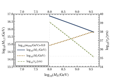
(a)

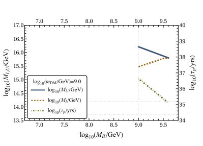
(c)

Figure 1: Plots of the unification scale $M_{U}$ and the first intermediate breaking scale $M_{I}$ along the $Y_{1}$-axis and the partial proton lifetime $\tau_{p}$ for the channel $p\to\pi^{0}e^{+}$ along the $Y_{2}$-axis as functions of the second intermediate breaking scale $M_{II}$ for different choices of the fermionic DM mass $m_{\rm DM}$ in the range $[10^{8},10^{9}]$ GeV. The horizontal dash-dotted lines correspond to the present Super-Kamiokande [46] and the projected Hyper-Kamiokande [47] limits on $\tau_{p}$. We see that the proton lifetime is only marginally within the reach of the future Hyper-Kamiokande experiment for a narrow range of $M_{II}$.

During the second intermediate symmetry breaking at $M_{II}$, the diagonal generator of $SU(2)_{R}$ combines with $(B-L)/2$ to give the SM hypercharge $Y$. The GUT normalization for $B-L$ and $Y$ is $\sqrt{3/8}$ and $\sqrt{3/5}$ respectively. Therefore, the matching condition reads

$$\frac{1}{\alpha_{Y}(M_{II})} =\frac{3}{5}\left(\frac{1}{\alpha_{2R}(M_{II})}-\frac{1}{6\pi}\right)+\frac{2}{5}\frac{1}{\alpha_{B-L}(M_{II})}-\frac{\lambda_{Y}(M_{II})}{12\pi}\ .$$ (11)

Fig. 3 shows the unification solutions of the model with the simplified assumption that the heavy multiplets that decoupled during the successive symmetry breakings are degenerate with the respective breaking scale. In this case, the threshold corrections given in the Appendix vanish. We see that in this case, the proton lifetime is only marginally within the reach of future experiments.

We next study the non-trivial effect of the threshold corrections assuming that the heavy multiplets are not degenerate with the respective breaking scales [48, 49, 50, 51, 52, 53, 54, 55, 44, 56, 57, 45, 58]. The threshold corrections in the Appendix will then have non-zero contributions.

We next consider an effective dimension-5 operator. The renormalizable gauge kinetic term in $SO(10)$ is

$$\mathcal{L}_{\rm kin}=-\frac{1}{4C}{\rm Tr}(F^{\mu\nu}F_{\mu\nu}).$$ (12)

Here, $F^{\mu\nu}=F^{\mu\nu}_{i}T^{i}$ with $T^{i}$ being the generators of $SO(10)$ normalized as ${\rm Tr}(T^{i}T^{j})=C\delta^{ij}$. The $210$-dimensional scalar $\chi_{210}$ comes from the symmetric product of two adjoint representations of $SO(10)$, i.e. $210\subset(45\times 45)_{S}$. We can write an effective dimension-5 operator given by

$$\mathcal{L}_{\rm kin}^{\rm dim\text{-}5}=-\frac{\eta}{\Lambda}\Big{[}\frac{1}{4C}{\rm Tr}(F^{\mu\nu}\chi_{210}F_{\mu\nu})\Big{]}.$$ (13)

The cut-off scale $\Lambda$ in the Wilson coefficient $(\eta/\Lambda)$ of Eq. (13) could be of the order of the reduced Planck scale $m_{\rm Pl}$. As $\chi_{210}$ acquires a non-zero VEV, the operator in Eq. (13), in addition to the threshold corrections also modifies the unification boundary conditions [59, 60, 61, 62, 63, 64]:

$$g_{U}^{2}=g_{i}^{2}(M_{U})(1+\varepsilon\delta_{i}),$$ (14)

where $\varepsilon=\eta\left<\chi_{210}\right>/(2\Lambda)\sim\mathcal{O}(M_{U}/m_{\rm Pl})$, and the group-theoretic factors are $\delta_{2L}=1/\sqrt{2}$, $\delta_{2R}=-1/\sqrt{2}$, and $\delta_{4C}=0$.

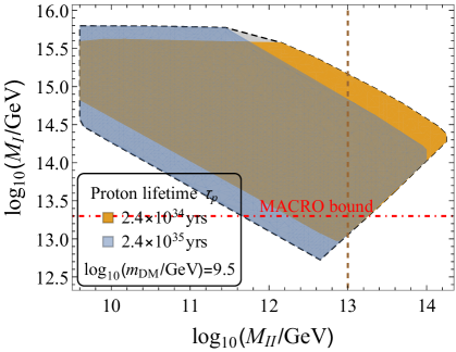
(c) $m_{S}/M_{i}\in[1/2,2]$ ($i=I,\ II$)

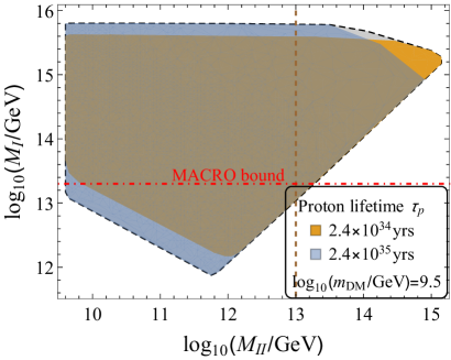
(d) $m_{S}/M_{i}\in[1/5,5]$

Figure 2: Plot for the intermediate scale $\log_{10}(M_{I}/\mathrm{GeV})$ versus $\log_{10}(M_{II}/\mathrm{GeV})$ with threshold corrections and dimension-5 operator included. In the upper panels, the unification scale is taken to be $\log_{10}(M_{U}/\mathrm{GeV})=16.51$ and the fermionic DM mass $\log_{10}(m_{\rm DM}/\mathrm{GeV})=9.5$. The MACRO bound [65] on the flux of the $SU(4)_{C}\times SU(2)_{L}\times SU(2)_{R}$ monopoles associated with the scale $M_{I}$ is also depicted (see Section 6). The vertical dashed line corresponds to $M_{II}\sim 10^{13}~{}{\rm GeV}$ which is suitable for leptogenesis (see Section 7). In the lower panels, we display the unification solutions with proton decay satisfying the Super-Kamiokande bound [46] and observable in the Hyper-Kamiokande experiment [47].

The upper panels of Fig. 3 show the solution region for successful inflation (see Section 5) with $\log_{10}(m_{\rm DM}/{\rm GeV})=9.5$ and $\log_{10}(M_{U}/{\rm GeV})=16.51$ after including the threshold corrections in Eqs. (3), (3), and (3) and the effect of the dimension-5 operator in Eq. (13). We assume that the heavy scalars have masses within $m_{S}/M_{i}\in[1/2,2]$ in panel (a) and $m_{S}/M_{i}\in[1/5,5]$ in panel (b) with $i=I,II,U$. The heavy multiplets in the daughter gauge symmetry which decouple are shown in Table 1. We can have unification solutions with a breaking scale $M_{II}\sim 10^{13}$ GeV (see Fig. 3), which is suitable for a successful leptogenesis as we will see in Section 7. The flux of the intermediate mass monopoles associated with the scale $M_{I}$ (see Section 6) can be measurable [66]. In the lower panels of Fig. 3, we display the unification solutions that yield proton decay lifetimes compatible with the Super-Kamiokande [46] bound and which could be observed in the Hyper-Kamiokande experiment [47]. The unification scale $M_{U}$ in this case ranges between about $4.5\times 10^{15}~{}{\rm GeV}$ and $7.5\times 10^{15}~{}{\rm GeV}$. Successful inflation (see Section 5) will then require large values of the relevant coupling constant.

5 Inflation with Coleman-Weinberg Potential

We consider inflation driven by the Coleman-Weinberg potential of a real GUT-singlet inflaton field $\phi$ [11, 67, 68, 69, 70]

$$V(\phi)=A\phi^{4}\left[\log\left(\frac{\phi}{M}\right)-\frac{1}{4}\right]+V_{0},$$ (15)

where $V_{0}=AM^{4}/4$ and the potential is minimized at $\phi=M$ with $V(\phi=M)=0$. Let us note in passing that a non-minimal coupling of the inflaton to gravity predicts smaller values for the tensor-to-scalar ratio $r$ [71, 72, 73, 14], which are preferred by the recent data [13] at $95\%$ confidence level.

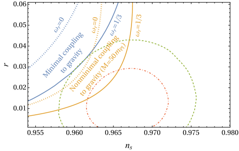
Figure 3: Predictions for $n_{\rm s}$ and $r$ for inflation driven by the Coleman-Weinberg potential of a real GUT singlet with minimal and nonminimal coupling to gravity. We take two values for $\omega_{r}$, the effective equation-of-state parameter from the end of inflation until reheating. The dot-dashed and dashed contours are the 68% and 95% confidence level contours of Planck TT, TE, EE + lowE + lensing + BK18 + BAO [13].

Fig. 3 compares the predictions for $n_{\rm s}$ and $r$ when the inflaton $\phi$ has minimal and nonminimal coupling to gravity. The 68% and 95% confidence level contours of Planck TT, TE, EE + lowE + lensing + BK18 + BAO [13] are also depicted. For nonminimal coupling to gravity, we have taken $M=50m_{\rm Pl}$ (for details see Ref. [14]). The interaction potential that induces the VEVs of the scalars at different symmetry-breaking scales is given by

$$V(\phi,\chi_{D})=-\frac{1}{2}\beta_{D}^{2}\phi^{2}\chi_{D}^{2}+\frac{\lambda_{D}}{4}\chi_{D}^{4},$$ (16)

where the symmetry-breaking scalars $\chi_{D}$ are canonically normalized real scalar fields with $D$ being the dimensionality of the representation to which $\chi_{D}$ belongs. The final VEVs are given by

$$\left<\chi_{D}\right>=(\beta_{D}/\sqrt{\lambda_{D}})M.$$ (17)

The interaction potential in Eq. (16) gives rise to the coefficient $A=\beta_{D}^{4}\,D/16\pi^{2}$ [74] in Eq. (15). This coefficient is dominated by the coupling $\beta_{210}$ of the scalar $\chi_{210}$ which acquires a non-zero VEV at $M_{U}$. Therefore, we can write

$$M_{U}\equiv\left<\chi_{210}\right>=\sqrt{\frac{8\pi}{\lambda_{210}}}\left(\frac{V_{0}}{210}\right)^{1/4}.$$ (18)

The effective mass squared of $\chi_{D}$ at the completion of the corresponding phase transition is given by

$$m_{\rm eff}^{2}=2(\beta_{D}^{2}\phi^{2}-\sigma_{\chi_{D}}T_{H}^{2}),$$ (19)

where $T_{H}=H/2\pi$ is the Hawking temperature during inflation with $H$ being the Hubble parameter and $\sigma_{\chi_{D}}\sim 1$. The completion of the phase transition is governed by the Ginzburg criterion $\xi^{3}\Delta V>T_{H}$ [75]. Here, $\xi\sim\mathrm{min}[H^{-1},m_{\rm eff}^{-1}]$ is the correlation length and $\Delta V=m_{\rm eff}^{4}/(16\lambda_{D})$ is the difference between the potential at $\chi_{D}=0$ and $\left<\chi_{D}\right>$. The phase transitions occur when

$$\beta_{D}\phi=\begin{cases}\sqrt{\left(128\lambda_{D}^{2}+\sigma_{\chi_{D}}\right)}\ \frac{H}{2\pi}&\mathrm{for}\ \ m_{\rm eff}^{-1}\lesssim H^{-1},\\ \sqrt{\left(4\pi\sqrt{2\pi\lambda_{D}}+\sigma_{\chi_{D}}\right)}\ \frac{H}{2\pi}&\mathrm{for}\ \ m_{\rm eff}^{-1}\gtrsim H^{-1}.\end{cases}$$ (20)

Successful inflation compatible with the Planck 2018 data [76] occurs for a typical choice $V_{0}^{1/4}=1.75\times 10^{16}$ GeV, $A=1.43\times 10^{-14}$, and $M=7.17\times 10^{19}$ GeV. The corresponding unification scale for $\lambda_{210}=1/2$ is $M_{U}=3.26\times 10^{16}$ GeV [8] as one can deduce from Eq. (18). For $M_{U}=7.5\times 10^{15}$ GeV, which may lead to proton lifetime measurable in Hyper-Kamiokande [47], the required value of $\lambda_{210}$ is 9.44.

6 Monopoles, Strings, and Gravitational Waves

The symmetry breaking scheme in Eq. (2) yields superheavy GUT monopoles of mass $\sim 10M_{U}$ [74, 66], intermediate scale monopoles of mass $\sim 10M_{I}$ [66], and topologically stable cosmic strings associated with the scale $M_{II}$ [6]. The dimensionless tension of the strings, in the Bogomol’nyi limit of the Abelian Higgs model, is given by

$$G\mu=\frac{1}{8}\left(\frac{\left<\phi_{126}\right>}{m_{\rm Pl}}\right)^{2},$$ (21)

where $G$ is Newton’s gravitational constant and we have $\left<\phi_{126}\right>=M_{II}$. These strings intercommute generating string loops that decay via the radiation of gravitational waves [77]. The production of gravitational waves from cosmic strings and related hybrid defects has been discussed in literature including Refs. [78, 79, 80, 81, 82, 83, 84, 85, 86, 87, 88, 89, 90, 91, 92, 93, 94, 95, 96, 97, 98, 99, 100].

The gravitational wave background at a frequency $f$ is given by [101, 102, 103, 104]

$$\Omega_{\rm GW}(f)=\frac{4\pi^{2}}{3H_{0}^{2}}f^{3}\int_{z_{*}}^{z(t_{F})}dz\int dl\,h^{2}(f,l,z)\frac{d^{2}R}{dz\,dl}\ ,$$ (22)

where the waveform assuming cusp domination is given by

$$h(f,l,z)=g_{1c}\frac{G\mu\,l^{2/3}}{(1+z)^{1/3}r(z)}f^{-4/3},$$ (23)

with $g_{1c}\simeq 0.85$ [104], $z$ being the redshift, and $l$ the loop length. The time $t_{F}$ corresponds to the onset of loop formation, and the lower limit $z_{*}$ in Eq. (22) excludes the infrequent bursts from the stochastic background such that [103]

$$\int_{0}^{z_{*}}dz\int dl\,\frac{d^{2}R}{dzdl}=f.$$ (24)

The proper distance $r$ is given by

$$r(z)=\int_{0}^{z}\frac{dz^{\prime}}{H(z^{\prime})},$$ (25)

where $H$ is the Hubble parameter with its present value denoted by $H_{0}$. The burst rate per unit space-time volume is given by

$$\frac{d^{2}R}{dz\,dl}=N_{c}H_{0}^{-3}\phi_{V}(z)\frac{2n(l,t(z))}{l(1+z)}\left(\frac{\theta_{m}(f,l,z)}{2}\right)^{2}\Theta(1-\theta_{m}),$$ (26)

where we have set $N_{c}=2.13$ as in Ref. [103], the beam opening angle

$$\theta_{m}(f,l,z)=\left[\frac{\sqrt{3}}{4}(1+z)fl\right]^{-1/3},$$ (27)

and

$$\phi_{V}(z)=\frac{4\pi H_{0}^{3}r^{2}}{(1+z)^{3}H(z)}\ .$$ (28)

In the radiation dominated universe the loop distribution function $n(l,t)$ at the time of gravitational wave emission is given by [105, 106]

$$n_{r}(l,t)=\frac{0.18}{t^{3/2}(l+\Gamma G\mu t)^{5/2}}\Theta(0.18t-l)\ .$$ (29)

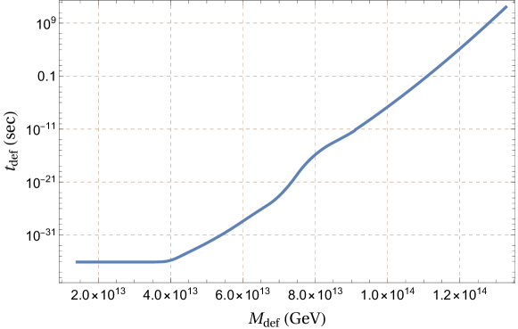
Figure 4: Horizon reentry time $t_{\rm def}$ of topological defects (strings or monopoles) formed during inflation as a function of the symmetry breaking scale $M_{\rm def}$.

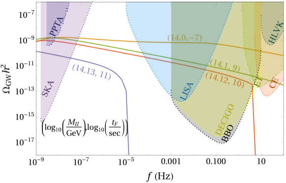
(b)

Figure 5: Gravitational wave spectra from cosmic strings generated during the spontaneous symmetry breaking at the scale $M_{II}$. The strings formed at the breaking scales $M_{II}\in[10^{9.65},10^{13.65}]$ GeV appear in the horizon at a very early cosmic time $t_{F}\lesssim 10^{-20}$ sec. The resulting gravitational wave background satisfies the present PPTA exclusion limit and can be probed by some of the proposed experiments. The strings formed during inflation around a breaking scale $1.3\times 10^{14}$ GeV reenter the horizon at $t_{F}\simeq 10^{11}$ sec and the gravitational wave spectrum from them satisfies the PPTA bound and can be probed by the SKA experiment. The sensitivity curves [107, 108] for PPTA [109] and various proposed experiments, including SKA [110, 111], CE [112], ET [113], LISA [114, 115], DECIGO [116], BBO [117, 118], HLVK [119], are also shown in the plots.

In the matter-dominated Universe, there are two contributions. For loops that are remnants from the radiation era,

$$n_{rm}(l,t)=\frac{0.18t_{eq}^{1/2}}{t^{2}(l+\Gamma G\mu t)^{2}}\Theta(0.18t_{eq}-l-\Gamma G\mu(t-t_{eq}))\ ,$$ (30)

where $t_{eq}$ is the equidensity time. For loops which are produced during the matter-dominated era,

$$n_{m}(l,t)=\frac{0.27-0.45(l/t)^{0.31}}{t^{2}(l+\Gamma G\mu t)^{2}}\Theta(0.18t-l)\Theta(l+\Gamma G\mu(t-t_{eq})-0.18t_{eq})\ .$$ (31)

We have taken the integration limits on $l$ to be from $0$ to $2t$ ($3t$) for radiation (matter) domination. However, the various Heaviside $\Theta$ functions will control the upper and lower limits during numerical evaluations.

Fig. 4 shows the horizon reentry time of topological defects such as strings or monopoles that are generated at the symmetry breaking scale $M_{II}$ or $M_{I}$ (call it $M_{\rm def}$) during inflation. Following the analysis of Ref. [99], we find that in our case inflation ends at a cosmic time $7.8\times 10^{-37}$ sec. Assuming $\lambda_{D}\sim g^{2}$ and using Eq. (20), we see that a spontaneous symmetry breaking occurs during inflation only if the breaking scale $M_{\rm def}\gtrsim 1.5\times 10^{13}$ GeV (see Refs. [8, 120] for more details). The gravitational wave spectra from the strings formed at the breaking scales $M_{II}\in[10^{9.65},10^{13.65}]$ GeV are shown in Fig. LABEL:fig:GWs-a. The present PPTA upper bound [109] is saturated for strings that are formed during inflation at the breaking scale $4.5\times 10^{13}$ GeV. In this case the strings reenter the horizon at a very early time $t_{F}<<t_{eq}\simeq 1.48\times 10^{12}$ sec as we can see from Fig. 4. Actually, in all cases depicted in Fig. LABEL:fig:GWs-a the strings are generated either during inflation and reenter the horizon at a very early time $t_{F}<<t_{eq}$, or during inflaton oscillations following the end of inflation at $t_{F}\lesssim 10^{-20}$ sec. Consequently, the gravitational wave spectrum remains unaffected by inflation in the nHz to kHz regime. Note that the phase transitions after the end of inflation are governed by the radiation temperature from the inflaton decay since this temperature soon outstrips the Hawking temperature (see Ref. [8]). The radiation temperature approaches the reheat temperature ($\sim 2\times 10^{6}$ GeV) at the reheat time $t_{r}\simeq 6.8\times 10^{-18}$ sec. We have checked that the contribution to the gravitational wave spectrum from the loops generated during inflaton oscillations is quite negligible in the frequency range under consideration and we therefore set $t_{F}=10^{-20}$ sec (see also Ref. [99]). Various proposed experiments, including the SKA [110, 111], CE [112], ET [113], LISA [114, 115], DECIGO [116], and BBO [117, 118] experiments, can observe this stochastic gravitational wave background. Fig. 5b shows the gravitational wave background for strings formed during inflation at the scales $M_{II}\gtrsim 4.5\times 10^{13}$ GeV. We see that the gravitational wave background from strings formed around a breaking scale $1.3\times 10^{14}$ GeV that reenter the horizon at $t_{F}\simeq 10^{11}$ sec is the only one satisfying the PPTA bound. This can be probed by the SKA experiment.

7 Non-thermal Dark Matter and Leptogenesis

The observed DM relic density can be realized in our setup non-thermally from the inflaton’s decay and axion. Moreover, the baryon asymmetry in the Universe can be generated via the right-handed neutrinos (RHNs) from the inflaton decay. The RHNs produce a primordial lepton asymmetry which is partially converted into the observed baryon asymmetry with the help of electroweak sphaleron effects. In practice, one needs to solve a set of coupled Boltzmann equations to investigate how these species evolve in the Universe. Following the prescription of Refs. [121, 122, 123], we construct the Boltzmann equations required for the analysis of the evolution of the different species involved in our setup.

Before delving into the details of Boltzmann equations, we would like to comment on the nature of the intermediate scale fermionic DM. The $\psi_{10}^{\alpha}~{}(\alpha=1,2)$ offer two neutral Dirac fermions, the lightest of which can play the role of DM stabilized by the unbroken $Z_{2}$ symmetry of $SO(10)$. The heavier color triplets and anti-triplets of the two 10-plets can decay into the $SU(2)_{L}$ doublet in the same 10-plet and SM particles via mediation of heavy lepto-quark gauge bosons [1, 124]. Apart from these, the charged members belonging to the $SU(2)_{L}$ doublets of these fermionic 10-plets can decay to the neutral components of the same doublet and SM particle – see Ref. [125] for details. It is interesting to point out that at the tree level, the two neutral fermions remain mass degenerate but a tiny non-zero mass splitting can be generated between them at the loop level. We refrain from going into the details of the calculation of this splitting and refer the reader to Refs. [126, 127, 128, 129, 130] for more details.

7.1 Boltzmann Equations

In this section, we provide a set of coupled Boltzmann equations for the time evolution of a system comprised of an unstable massive particle $\phi$ (inflaton) with mass $m_{\phi}$, unstable RHNs ($N_{i}$) with mass $M_{i}$, radiation (R), lepton number asymmetries generated in the visible sector ($n_{L_{i}}$) as a result of the decay of the RHNs $N_{i}$, and a stable massive fermion $\psi_{\rm DM}$ (the lightest neutral component of $\psi_{10}$) with mass $m_{\rm DM}$ which contributes to DM. In this scenario, it is assumed that $\phi$ decays predominantly to RHNs but also to stable DM fermions.

$$\frac{d\rho_{\phi}}{dt} = -3H\rho_{\phi}-\Gamma_{\phi}\rho_{\phi},$$ (32a)

$$\frac{d\rho_{N_{i}}}{dt} = -3H\rho_{N_{i}}+\Gamma_{\phi\to N_{i}N_{i}}\rho_{\phi}-\Gamma_{N_{i}}\rho_{N_{i}},$$ (32b)

$$\frac{d\rho_{\rm R}}{dt} = -4H\rho_{\rm R}+\sum_{i=1,2,3}\Gamma_{N_{i}}\rho_{N_{i}}+\langle\sigma v\rangle 2\langle E_{\psi_{\rm DM}}\rangle n_{\psi_{\rm DM}}^{2},$$ (32c)

$$\frac{dn_{L_{i}}}{dt} = -3Hn_{L_{i}}+\epsilon_{i}\Gamma_{N_{i}}n_{N_{i}},$$ (32d)

$$\frac{dn_{\psi_{\rm DM}}}{dt} = -3Hn_{\psi_{\rm DM}}+\Gamma_{\phi\to\psi_{\rm DM}\psi_{\rm DM}}\frac{\rho_{\phi}}{m_{\phi}}-\langle\sigma v\rangle n_{\psi_{\rm DM}}^{2}.$$ (32e)

Here $\rho_{i}$ and $n_{i}$ represent the energy and the number densities of the particles under consideration, $\Gamma_{\phi}=\Gamma_{\phi\to N_{i}N_{i}}+\Gamma_{\phi\to\psi_{\rm DM}\psi_{\rm DM}}$ denotes the total decay width of the inflaton, where

$$\Gamma_{\phi\to N_{i}N_{i}}=\frac{1}{16\pi}\bigg{(}\frac{M_{i}}{M}\frac{m_{126}^{2}}{m_{\phi}^{2}}\bigg{)}^{2}m_{\phi}\quad{\rm and}\quad\Gamma_{\phi\to\psi_{\rm DM}\psi_{\rm DM}}=\frac{10}{16\pi}\bigg{(}\frac{m_{\rm DM}}{M}\frac{m_{45}^{2}}{m_{\phi}^{2}}\bigg{)}^{2}m_{\phi}$$ (33)

are the decay widths of the inflaton to RHNs and fermionic DM respectively (see Ref. [1]) with $m_{126}$ and $m_{45}$ being the intermediate scale masses of $\phi_{126}$ and $\phi_{45}$. Also $\Gamma_{N_{i}}=(1/8\pi)(y_{\nu}^{\dagger}y_{\nu})_{ii}M_{i}$ are the decay widths of the RHNs with $y_{\nu}$ being the neutrino Yukawa coupling matrix in the basis where the RHN masses are diagonal. The Hubble parameter is $H=\dot{a}/a$, where $a$ denotes the scale factor of the Universe and the overdot the time derivative. Moreover, $\langle\sigma v\rangle$ corresponds to the thermal average of the annihilation cross section times the velocity of the DM fermions and we assumed that each DM fermion has energy $\langle E_{\psi_{\rm DM}}\rangle$ (with $\rho_{\psi_{\rm DM}}=\langle E_{\psi_{\rm DM}}\rangle n_{\psi_{\rm DM}}$). Finally, the lepton asymmetry ($\epsilon_{i}$) generated by the decay of a RHN $N_{i}$ is given as [131]

$$\epsilon_{i}=\frac{1}{8\pi}\frac{\text{Im}[(y_{\nu}^{\dagger}y_{\nu})^{2}_{ij}]}{(y_{\nu}^{\dagger}y_{\nu})_{ii}}\mathcal{F}\left(\frac{M_{j}^{2}}{M_{i}^{2}}\right),$$ (34)

where $\mathcal{F}(x)=\sqrt{x}\bigg{[}1+\frac{1}{1-x}+(1+x)\ln(\frac{x}{1+x})\bigg{]}$.

In Eq. (32a) we show the evolution of the inflaton energy density. The first term in the right-hand side (RHS) of this equation is responsible for the dilution of the inflaton energy density due to the expansion of the Universe, and the second term accounts for the reduction of this energy density due to the inflaton decay. Eq. (32b) describes the evolution of the energy density of the RHNs. Here the first term in the RHS again shows the dilution effect due to the expansion of the Universe, the second term is due to the production of the RHN from the decay of the inflaton (hence the positive sign), and the third term accounts for the depletion (negative sign) of the RHN energy density due to its decay into SM particles. Next, we provide the evolution of the radiation energy density in Eq. (32c). Here, the first term in the RHS represents the dilution of the radiation energy density due to the expansion and comes with a factor of 4 rather than 3 because the radiation energy density scales as $\rho_{R}\propto a^{-4}$. The second term depicts the production of radiation from the decay of the RHNs, and the third term shows the contribution coming from the annihilation of DM fermions into radiation with the factor of 2$\langle E_{\psi_{\rm DM}}\rangle$ being the average energy released in a pair annihilation of DM fermions. In Eq. (32d) we show the evolution of the lepton number asymmetry $n_{L_{i}}$ generated in the visible sector due to the decay of the RHN $N_{i}$ to SM particles (leptons and Higgs bosons). Note that, since we aim to analyze a non-thermal leptogenesis scenario where the reheat temperature $T_{RH}<<M_{i}$, the washout of the asymmetries due to the inverse decay can safely be ignored as the thermal bath does not have sufficient energy to reproduce RHNs. Finally, in Eq. (32e) we provide the evolution of the number density of the DM fermions ($n_{\psi_{\rm DM}}$). The second term in the RHS of this equation is responsible for the production of DM fermions from the decay of the inflaton, and the third term describes the reduction of the number density of the DM fermions due to their annihilation.

7.2 Transformation of variables and initial conditions

In solving the Boltzmann equations, it is useful to use quantities in which the expansion of the Universe is scaled out. Here, we use the following transformation of the variables

$$E_{\phi} = \rho_{\phi}a^{3},$$ (35a)

$$E_{N_{i}} = \rho_{N_{i}}a^{3},$$ (35b)

$$N_{L_{i}} = n_{L_{i}}a^{3},$$ (35c)

$$R = \rho_{\rm R}a^{4},$$ (35d)

$$X = n_{\psi_{\rm DM}}a^{3}.$$ (35e)

We next define the dimensionless quantity $y$ in terms of the scale factor ($a$) and its initial value ($a_{I}$):

$$y\equiv\frac{a}{a_{I}}.$$ (36)

The Hubble parameter of the Universe can be written as

$$H = \sqrt{\frac{1}{3m_{\rm Pl}^{2}}\bigg{(}\rho_{\phi}+\sum_{i=1,2,3}\rho_{N_{i}}+\rho_{\rm R}\bigg{)}}$$ (37)

$$= \sqrt{\frac{1}{3m_{\rm Pl}^{2}a_{I}^{4}y^{4}}\bigg{(}E_{\phi}a_{I}y+\sum_{i=1,2,3}E_{N_{i}}a_{I}y+R\bigg{)}}.$$

Using the rescaled variables, one can rewrite the set of Boltzmann equations in Eq. (32) as

$$E_{\phi}^{\prime} = -\frac{\Gamma_{\phi}}{H}\frac{E_{\phi}}{y},$$ (38a)

$$E_{N_{i}}^{\prime} = \frac{1}{Hy}(\Gamma_{\phi\to N_{i}N_{i}}E_{\phi}-\Gamma_{N_{i}}E_{N_{i}}),$$ (38b)

$$N_{L_{i}}^{\prime} = \frac{1}{Hy}\epsilon_{i}\Gamma_{N_{i}}N_{i},$$ (38c)

$$R^{\prime} = \frac{1}{H}\sum_{i=1,2,3}\Gamma_{N_{i}}E_{N_{i}}a_{I},$$ (38d)

$$X^{\prime} = \frac{1}{Hy}\Gamma_{\phi\to\psi_{\rm DM}\psi_{\rm DM}}\frac{E_{\phi}}{m_{\phi}},$$ (38e)

where the prime denotes derivation with respect to $y$.

At very early cosmic times, the energy density of the inflaton dominates the Universe with the initial number or energy density of the rest of the contents of the Universe being zero. The initial value of the $\phi$ energy density can be expressed in terms of the initial expansion rate $H_{I}$ as $\rho_{\phi_{I}}=3m_{\rm Pl}^{2}H_{I}^{2}$. Hence, we set the initial values of the variables appearing in Eq. (38) as

$$E_{\phi_{I}}=3m_{\rm Pl}^{2}H_{I}^{2}a_{I},$$ (39)

and

$$E_{N_{i}}=0,~{}~{}R_{I}=0,~{}~{}N_{L_{i}}=0,~{}~{}X=0.$$ (40)

Note that since we are interested in exploring non-thermal leptogenesis together with non-thermal production of fermionic DM, we must keep in mind that the heavy RHNs ($N_{i}$) and the DM candidate $\psi_{\rm DM}$ are never in thermal equilibrium with the thermal bath ($\rho_{N_{i}}^{\rm eq}=0$ and $n_{\psi_{\rm DM}}^{\rm eq}=0$). As we are interested in quite heavy ($\sim f_{a}$) DM fermions, we may safely ignore the terms corresponding to DM annihilation in Eq. (32e) and also in the production of radiation in Eq. (32c) since the DM annihilation cross-sections will be highly suppressed. Such suppressed cross-sections guarantee that the pair annihilation of DM remains out of equilibrium $i.e.~{}n_{\psi_{\text{DM}}}\langle\sigma v\rangle\lesssim H$ (as was also shown and discussed in Ref. [1]) at any temperature smaller than the reheat temperature and hence the DM abundance remains constant. Finally, the direct decay of the inflaton to radiation is very small and hence can be neglected in Eq. (32c).

One can express the final primordial lepton asymmetry yields $Y_{L_{i}}$ in terms of $N_{L_{i}}$ as

$$Y_{L_{i}}=\frac{n_{L_{i}}}{s}=\bigg{(}\frac{45}{2\pi^{2}g_{*s}}\bigg{)}\bigg{(}\frac{\pi^{2}g_{*}}{30}\bigg{)}^{3/4}N_{L_{i}}R^{-3/4},$$ (41)

where $s=(2\pi^{2}/45)g_{*s}T^{3}$ represents the entropy density with $T=(30/g_{*}\pi^{2})^{1/4}\rho_{R}^{1/4}$ being the cosmic temperature. Here, $g_{*}$ ($g_{*s}$) is the effective number of massless degrees of freedom for the energy (entropy) density. Finally, the baryon asymmetry yield can be expressed as

$$Y_{B}=-\frac{28}{79}\sum_{i=1,2,3}Y_{L_{i}}.$$ (42)

Similarly, the fermionic DM relic abundance is

$$\Omega_{\psi_{\rm DM}}h^{2} = 2\times 2.75\times 10^{8}\bigg{(}\frac{m_{\rm DM}}{\rm GeV}\bigg{)}Y_{\psi_{\rm DM}}$$ (43)

$$= 2.75\times 10^{8}\bigg{(}\frac{45}{2\pi^{2}g_{*s}}\bigg{)}\bigg{(}\frac{\pi^{2}g_{*}}{30}\bigg{)}^{3/4}\bigg{(}\frac{m_{\rm DM}}{\rm GeV}\bigg{)}XR^{-3/4},$$

where $Y_{\psi_{\rm DM}}=n_{\psi_{\rm DM}}/s$ is the fermionic DM yield.

8 Numerical Analysis

Before delving into the detailed solution of Boltzmann equations, we would like to briefly discuss the possibility of axion as a DM candidate in the present model. Clearly, the axion being a integral part of this model can also contribute to the DM relic density, but its contribution depends on the choice of the PQ breaking scale $f_{a}$. The relic axion abundance is expressed as [132]

$$\Omega_{a}h^{2}=\Omega_{a}^{mis}h^{2}+\Omega_{a}^{str}h^{2}\simeq 2.41\bigg{(}\frac{f_{a}}{10^{12}~{}\text{GeV}}\bigg{)}^{7/6},$$ (44)

where $\Omega_{a}^{mis}h^{2}$ and $\Omega_{a}^{str}h^{2}$ represent the contributions coming from the misalignment mechanism [133, 134, 135, 132] and the decay of axionic strings [136, 132], respectively. The relic axion abundance produced by the misalignment mechanism is [132]

$$\Omega_{a}h^{2}\simeq 0.236\bigg{(}\frac{f_{a}}{10^{12}~{}\text{GeV}}\bigg{)}^{7/6}\langle\theta^{2}f(\theta)\rangle,$$ (45)

where $\theta$ denotes the misalignment angle that lies in the interval $[-\pi,\pi]$ [137]. The function $f(\theta)$ incorporates the anharmonicity of the axion potential and the mean value $\langle\theta^{2}f(\theta)\rangle$ evaluated in the interval $[-\pi,\pi]$ turns out to be around 8.77 [132]. On the other hand, the contribution coming from the decay of axionic strings is given by [132]

$$\Omega_{a}^{str}h^{2}\simeq 0.34\bigg{(}\frac{f_{a}}{10^{12}~{}\text{GeV}}\bigg{)}^{7/6}.$$ (46)

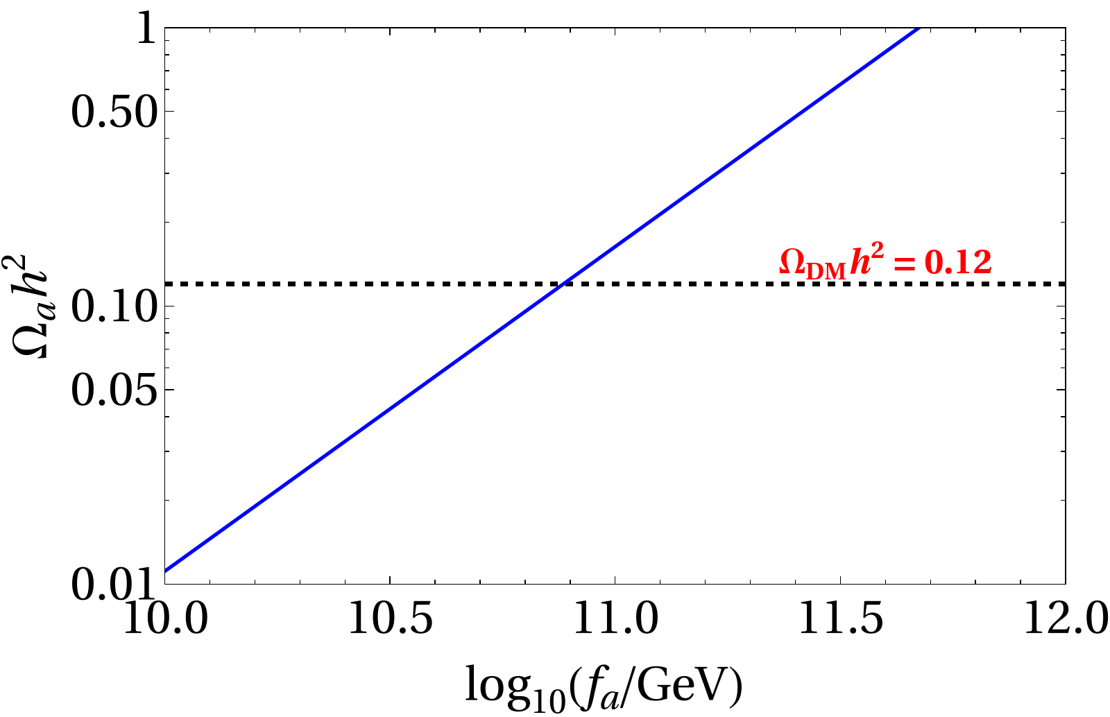
Figure 6: Variation of axion relic abundance with the axion decay constant $f_{a}$. The black dashed line corresponds to $\Omega_{\text{DM}}h^{2}=0.12$.

In Fig. 6, we show the variation of the axion relic abundance $\Omega_{a}h^{2}$ with the axion decay constant $f_{a}$. The black dashed line corresponds to the Planck limit [138] on the total relic DM abundance $\Omega_{\text{DM}}h^{2}$. Note that with $f_{a}\simeq 8\times 10^{10}$ GeV, the axion alone can contribute $100\%$ of the relic abundance of DM. The constraint on the relic DM abundance also gives an upper bound on $f_{a}$, suggesting that with $f_{a}>8\times 10^{10}$ GeV the axion can over-close the energy density of the Universe. The total DM relic abundance that should satisfy the Planck limit [138] must include the contribution from the lightest neutral component of $\psi_{10}$:

$$\Omega_{\rm DM}h^{2}=\Omega_{a}h^{2}+\Omega_{\psi_{\rm DM}}h^{2}.$$ (47)

Next, we discuss the solution of the Boltzmann equations. To solve them, we need to have information about the masses and couplings of the various species involved. To this end, we first demonstrate how we obtain the masses of the different RHNs and their corresponding Yukawa couplings. The Lagrangian for the Yukawa interactions of the SM fermions and RHNs is given by

$$y_{10}\psi_{16}^{\rm T}\mathcal{C}\phi_{10}\psi_{16}+y_{126}\psi_{16}^{\rm T}\mathcal{C}\phi_{126}^{\dagger}\psi_{16}+{\rm H.c.},$$ (48)

where the transpose $T$ and the charge conjugation operator $\mathcal{C}:{\psi^{C}}_{L,R}\equiv\mathcal{C}\bar{\psi}_{R,L}^{\rm T}$ act in the Dirac space of each left ($L$) or right handed ($R$) fermionic field, and $y_{10}$, $y_{126}$ are $3\times 3$ matrices in the family space. The VEVs of the four $SU(2)_{L}$ doublets from the $(2,2,1)$ component of $\phi_{10}$ and the $(2,2,15)$ component of $\phi_{126}^{\dagger}$ are $v_{10}^{u}$, $v_{10}^{d}$, $v_{126}^{u}$, and $v_{126}^{d}$ with the superscripts $u$ and $d$ referring to the up-type and down-type components. The SM Yukawa couplings for the up-and down-type quarks, neutrinos, and charged leptons are [139, 140]

$$y_{u} =\frac{1}{v_{\rm SM}}\left(v_{10}^{u}y_{10}+v_{126}^{u}y_{126}\right),$$

$$y_{d} =\frac{1}{v_{\rm SM}}\left(v_{10}^{d}y_{10}+v_{126}^{d}y_{126}\right),$$

$$y_{\nu} =\frac{1}{v_{\rm SM}}\left(v_{10}^{u}y_{10}-3v_{126}^{u}y_{126}\right),$$

$$y_{l} =\frac{1}{v_{\rm SM}}\left(v_{10}^{d}y_{10}-3v_{126}^{d}y_{126}\right),$$ (49)

where $v_{\rm SM}$ is the SM breaking VEV. The Majorana mass matrix of the RHNs after the $(1,3,10)\in\overline{126}$ acquires its VEV ($v_{R}$) at the scale $M_{II}$ is expressed as

$$M_{R}=y_{126}v_{R}.$$ (50)

We adopt the parametrization $h\equiv(v_{10}^{d}/v_{\rm SM})y_{10}$, $f\equiv(v_{126}^{d}/v_{\rm SM})y_{126}$, $r\equiv(v_{10}^{u}/v_{10}^{d})$, $s\equiv(1/r)(v_{126}^{u}/v_{126}^{d})$, $r_{R}\equiv v_{R}(v_{\rm SM}/v_{126}^{d})$, and re-express the Yukawa couplings as

$$y_{u} =r(h+sf),$$

$$y_{d} =h+f,$$

$$y_{\nu} =r(h-3sf),$$

$$y_{l} =h-3f.$$ (51)

The RHN mass matrix takes the form

$$M_{R}=r_{R}f.$$ (52)

To estimate the baryon asymmetry of the Universe we need the RHN masses and the Dirac Yukawa couplings ($y_{\nu}$) of the neutrinos in the diagonal basis of the RHN mass matrix ($M_{R}$) and the charged lepton Yukawa coupling matrix ($y_{l}$). The fit of the renormalizable Yukawa couplings to fermion masses and mixings at the electroweak scale has been extensively studied in several papers [141, 142, 143, 144, 145, 146, 147, 148, 149, 150, 151]. We use the best fit Yukawa couplings with the scalars $10_{H}\oplus\overline{126}_{H}$ in the $SO(10)\times U(1)_{\rm PQ}$ GUT model from two recent references [150, 151], and we run the fitted couplings from the GUT scale ($\sim 10^{16}$ GeV) to the intermediate scale ($\sim 10^{12}$ GeV) using the SM RGEs given in Ref. [150]. At the scale $10^{12}$ GeV, we diagonalize the RHN mass matrix and compute the Dirac Yukawa coupling matrix $y_{\nu}$ in the same basis where the RHN mass matrix $M_{R}$ and the charged lepton Yukawa coupling matrix $y_{l}$ are diagonal:

$$M_{R}^{\rm D}=U_{R}M_{R}U_{R}^{\rm T},\ y_{l}^{\rm D}=U_{l}y_{l}{U_{l}^{c}}^{\dagger}\Rightarrow y_{\nu}\to U_{l}y_{\nu}U_{R}^{*}.$$ (53)

8.1 Examples

Example I: The fitted parameters in Ref. [150] are

$$h =\begin{pmatrix}0.0001&0&0\\ 0&0.0556&0\\ 0&0&6.5110\\ \end{pmatrix}\times 10^{-3},$$

$$f =\begin{pmatrix}0.00556-0.00318i&-0.01130-0.01208i&-0.03546-0.14594i\\ -0.01130-0.01208i&-0.16392+0.03471i&-0.25650+0.25582i\\ -0.03546-0.14594i&-0.25650+0.25582i&-0.91962-0.50277i\end{pmatrix}\times 10^{-3},$$

$$r =-65.9350{\rm,}\ s=0.391447-9.585\times 10^{-17}i{\rm,}\ r_{R}=2.04454\times 10^{15}\ {\rm GeV.}$$ (54)

The physical masses of the RHNs are obtained as

$$M_{R}^{D}=\left\{1.87\times 10^{10},4.46\times 10^{11},2.36\times 10^{12}\right\}\ \mathrm{GeV},$$ (55)

and the Dirac Yukawa structure of the light neutrinos in the basis described in Eq. (53) is given by

$$U_{l}y_{\nu}U_{R}^{*}=\begin{pmatrix}-0.00123+0.00077i&0.00261+0.00204i&-0.00258+0.01029i\\ -0.00229-0.00012i&-0.00629+0.01499i&-0.00719+0.03334i\\ -0.05876+0.03800i&0.08977+0.07709i&-0.15355+0.45175i\end{pmatrix}.$$ (56)

Next, we plug these values of the RHN masses and the Yukawa couplings into the Boltzmann equations (Eq. (38)) and we also fix $m_{\phi}=1.7\times 10^{13}~{}\text{GeV}$ corresponding to the parameter values for successful inflation in Section 5 [1] and $m_{126}=7.5\times 10^{12}$ GeV. These values of $m_{\phi}$ and $m_{126}$ together with the given RHN masses are chosen to obtain the baryon asymmetry’s desired value. Form Fig. 6 one sees that depending on the choice of the axion decay constant $f_{a}$, the axion can fully account for or partially contribute to the DM relic abundance. With this in mind, we set $f_{a}\simeq m_{45}=5\times 10^{10}$ GeV, such that the axion contributes $\sim 60\%$ ($\Omega_{a}h^{2}=0.073$) of the DM relic abundance, and the remaining $40\%$ comes from the fermionic component.

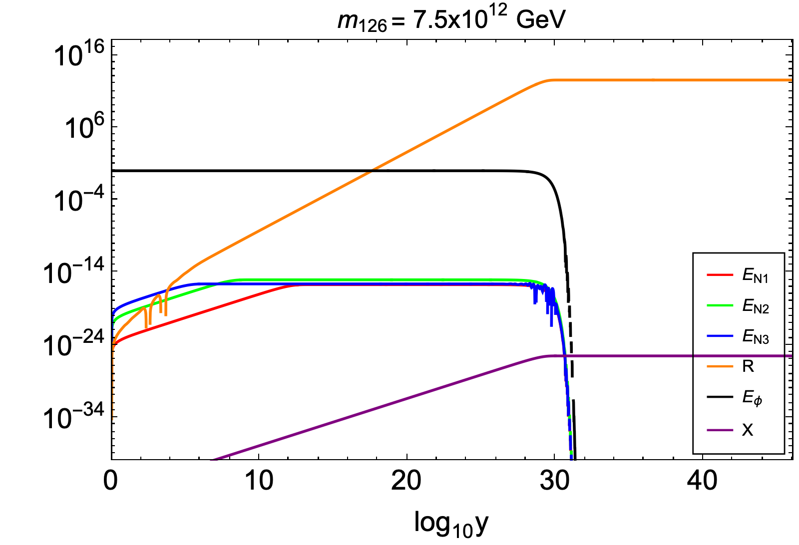
Figure 7: Evolution of the rescaled energy and number densities of the various components in the Universe (normalized to $E_{\phi_{I}}$ ) versus $\log_{10}y$ for fixed values of $m_{\phi}=1.7\times 10^{13}~{}\text{GeV}$ and $m_{126}=7.5\times 10^{12}$ GeV. Here we have set $m_{\rm DM}=7\times 10^{9}$ GeV and $m_{45}=5\times 10^{10}$ GeV such that $\Omega_{\psi_{\rm DM}}h^{2}=0.046$.

(a)

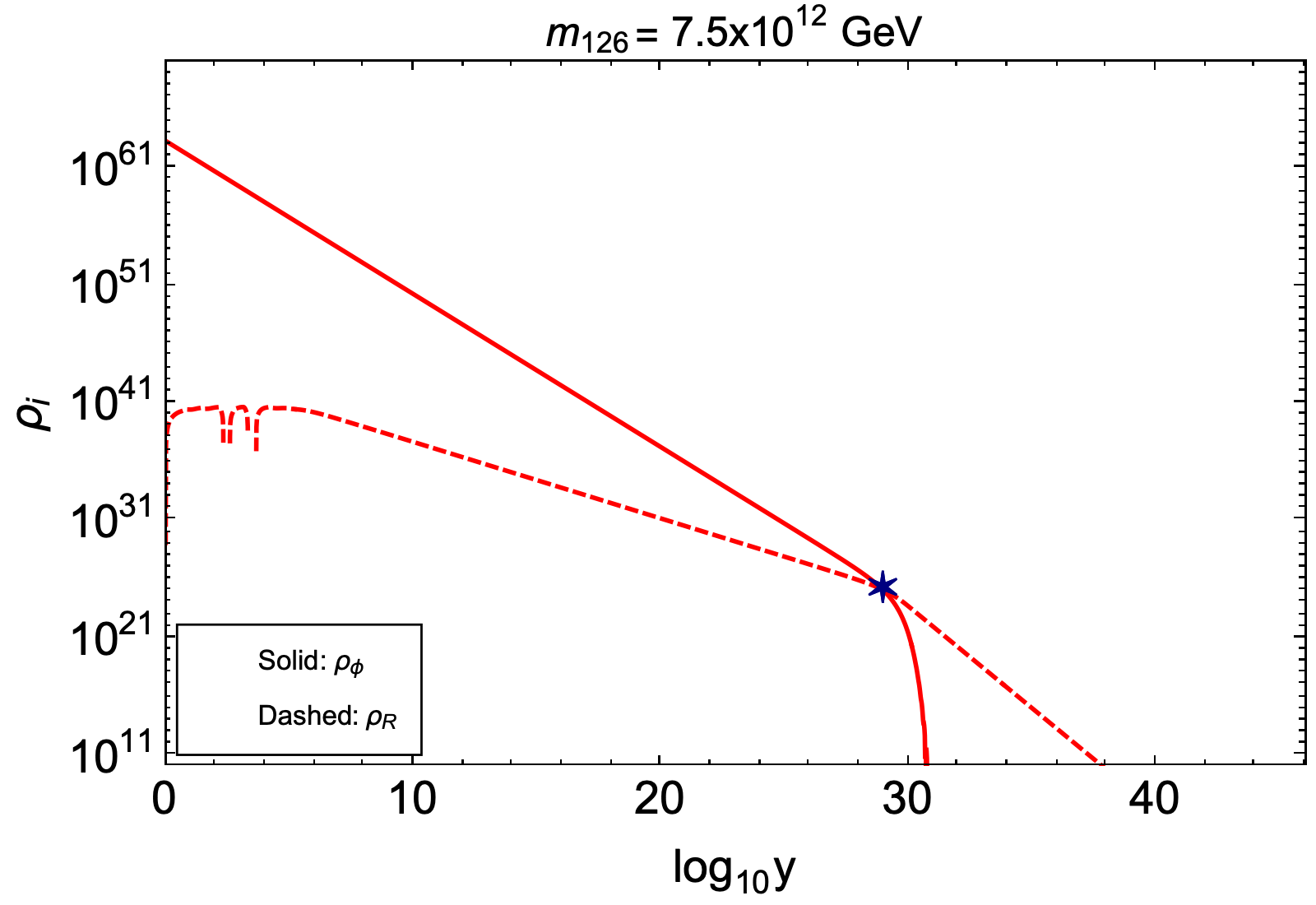
(c)

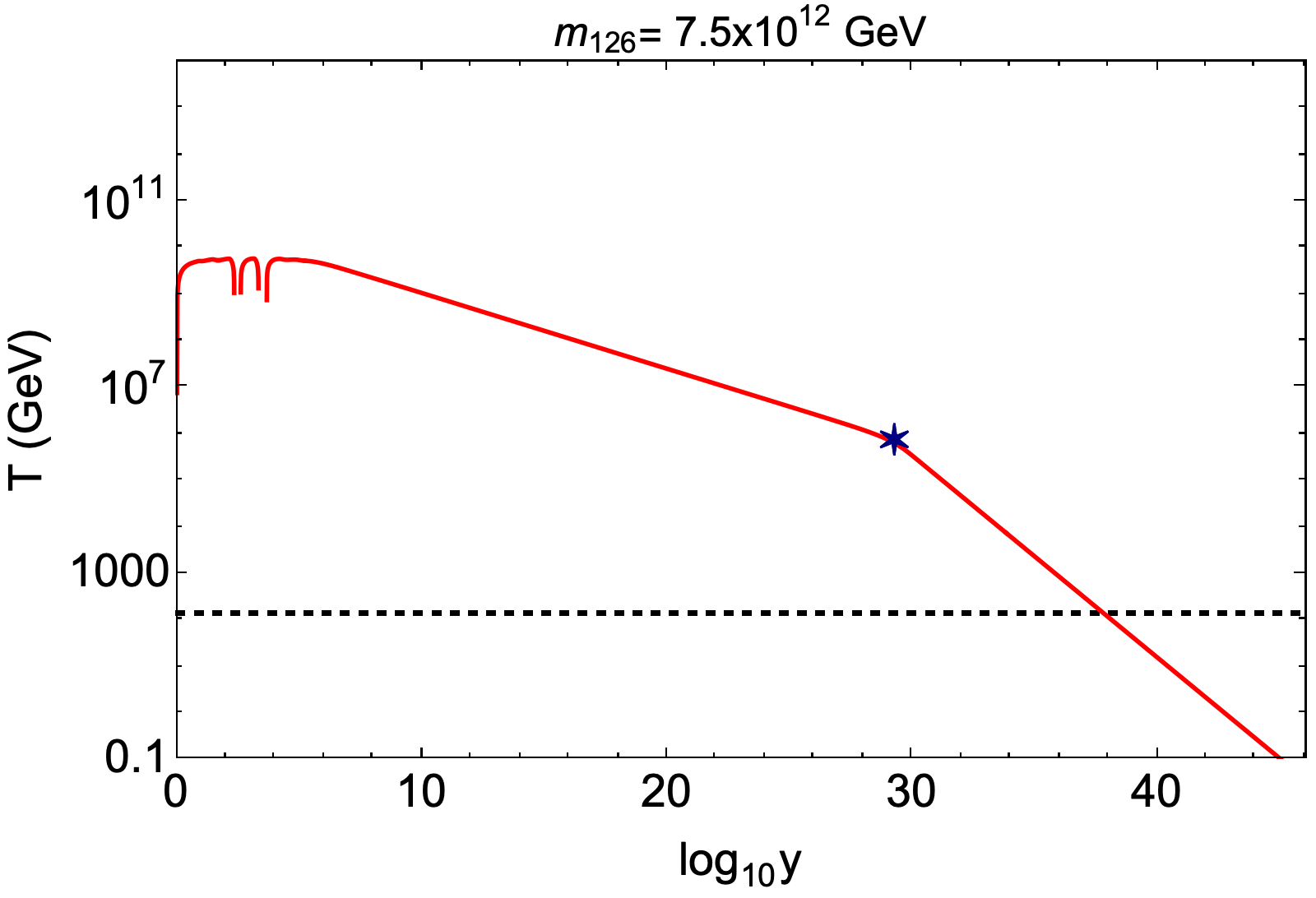
(d)

Figure 8: Top left panel: evolution of the rescaled energy densities of all three RHNs together with the corresponding lepton asymmetries (normalized to $E_{\phi_{I}}$ ) as functions of $\log_{10}y$. Top right plot: evolution of the individual lepton asymmetry yields together with the total asymmetry. The horizontal dashed line corresponds to the total primordial lepton asymmetry ($Y_{L}\simeq 2.5\times 10^{-10}$) that gives the observed baryon asymmetry of the Universe ($Y_{B}\simeq 8.7\times 10^{-11}$). Bottom left panel: evolution of $\rho_{\phi}$ and $\rho_{R}$ with $\log_{10}y$. The $\star$ mark shows the cross-over of $\rho_{\phi}$ and $\rho_{R}$. Bottom right panel: evolution of the bath’s temperature with $\log_{10}y$. Here the $\star$ mark corresponds to $T_{RH}$ and the horizontal dashed line shows the sphaleron free-out temperature $T_{sph}\simeq 130$ GeV. All these plots are made for a fixed value of $m_{\phi}=1.7\times 10^{13}~{}\text{GeV}$ and $m_{126}=7.5\times 10^{12}$ GeV.

Solving the Boltzmann equations we find the evolution of the different species, which are crucial for baryon asymmetry and the DM abundance in the Universe, as functions of the dimensionless quantity $y=a/a_{I}$ where we have set $a_{I}=1$ [121]. The results are depicted in Fig. 7. All these rescaled energy and number densities are normalized by the initial energy density of the inflaton $E_{\phi_{I}}$. Here, the black line corresponds to the inflaton, and the red, green, and blue lines to the RHNs $N_{1}$, $N_{2}$, and $N_{3}$ respectively. The orange and purple lines respectively correspond to the radiation and the fermionic DM. One notices that the rescaled inflaton energy density initially remains constant but, at $\log_{10}y\simeq 30$, completely decays to RHNs and fermionic DM. As expected, the fermionic DM rescaled number density slowly increases as a result of its production from the inflaton decay until the point when the decay of the inflaton is completed. Thereafter, it remains constant giving rise to the final fermionic DM abundance that corresponds to almost $40\%$ of the DM relic abundance of the Universe for $m_{\rm DM}=7\times 10^{9}$ GeV. The RHN rescaled energy densities also gradually increase due to their production by the inflaton decay and are subsequently stabilized when their production rate from the inflaton decay becomes comparable to their decay rate to SM particles. Being the heaviest among all RHNs, $N_{3}$ has the largest decay width ($\Gamma_{N_{3}}\propto M_{3}$). Consequently, the rescaled energy density of $N_{3}$ is stabilized much earlier than that of the other two RHNs. It is interesting to point out that the decay of the RHNs is almost completed at the same time as that of the inflaton. This is because the RHNs decay instantaneously after their production as $\Gamma_{N_{i}}>>\Gamma_{\phi}$ in all cases. As a result of the RHN decay, a rise in the rescaled radiation energy density is also observed. The production of radiation stops once all the RHNs have completely decayed.

In the top left panel of Fig. 3, we show the evolution of the rescaled energy densities of the RHNs and the lepton asymmetries (scaled by $E_{\phi_{I}}$) generated by their CP-violating decays. The behavior of these asymmetries is similar to that of radiation in Fig. 7. In the top right panel of Fig. 3, we plot the absolute values of the lepton asymmetry yields ($Y_{L_{i}}=n_{L_{i}}/s$) generated by the decay of the RHNs together with the absolute value of the total lepton asymmetry yield (shown in magenta) which leads, for large values of $y$, to the primordial lepton asymmetry (shown by the black dashed line) required to produce the observed baryon asymmetry of the Universe. The dip observed in the total lepton asymmetry $Y_{L}$ is a result of cancellation due to the different signs of the individual lepton asymmetries generated in the decay of the RHNs. The decrease of these asymmetries after some point is caused by the entropy injection into the bath. This happens when the decay rates of the RHNs become comparable to their production rates and as a result, the radiation starts to build at a faster rate as can also be seen from Fig. 3. Finally, the asymmetries stabilize once the decay of the RHNs is complete. In the bottom left panel of Fig. 3 we show the evolution of the energy densities of the inflaton $\rho_{\phi}$ (red solid) and the radiation $\rho_{R}$ (red dashed). This plot shows that the radiation-dominated era starts only when $\rho_{R}=\rho_{\phi}$ is reached, and we use this condition to determine the Universe’s reheat temperature ($T_{RH}$). In the bottom right plot of Fig. 3 we show the evolution of the thermal bath’s temperature given by

$$T_{R}=\bigg{(}\frac{30}{g_{*}\pi^{2}}\bigg{)}^{1/4}\rho_{R}^{1/4},$$ (57)

where $g_{*}=106$. For the above choices of parameters, the reheat temperature of the Universe is found to be $T_{RH}=1.9\times 10^{6}$ GeV (shown by the $\star$). Here, we also show a black dashed horizontal line that corresponds to the sphaleron freeze-out temperature $T_{sph}=130$ GeV [152, 153, 154].

Example II: The fitted parameters in Ref. [151] are

$$h =\begin{pmatrix}0.00023&0&0\\ 0&-0.04811&0\\ 0&0&-5.79504\\ \end{pmatrix}\times 10^{-3},$$

$$f =\begin{pmatrix}-0.00088+0.00178i&0.00475-0.00889i&0.04635+0.06797i\\ 0.00475-0.00889i&0.11279+0.05108i&-0.12218-0.25921i\\ 0.04635+0.06797i&-0.12218-0.25921i&0.54683-0.59856i\\ \end{pmatrix}\times 10^{-3},$$

$$r =77.4189{\rm,}\ s=0.314-0.0282i{\rm,}\ r_{R}=9.84\times 10^{14}\ {\rm GeV.}$$ (58)

At the scale $10^{12}$ GeV, we have diagonalized the RHN mass matrix and computed the Dirac Yukawa matrix $y_{\nu}$ in the basis where the RHN mass matrix ($M_{R}$) and the charged lepton Yukawa coupling matrix ($y_{l}$) are diagonal.

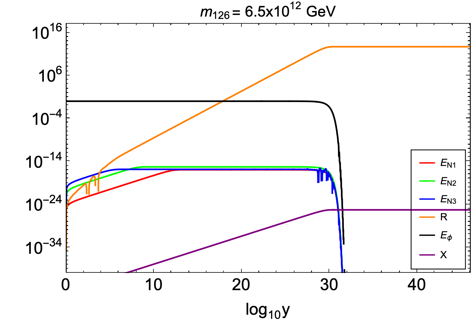
(a)

Figure 9: Left panel: evolution of the rescaled energy and number densities of various components (normalized to $E_{\phi_{I}}$ ) as functions of $\log_{10}y$ for fixed values of $m_{\phi}=1.7\times 10^{13}~{}\text{GeV}$ and $m_{126}=6.5\times 10^{12}$ GeV. Here we have set $m_{\rm DM}=4.5\times 10^{9}$ GeV and $m_{45}=5\times 10^{10}$ GeV such that $\Omega_{\psi_{\rm DM}}h^{2}=0.041$. Consequently, the fermionic DM contributes $34\%$ of the DM in the Universe. Right panel: evolution of the individual lepton asymmetry yields together with the total asymmetry. The horizontal dashed line corresponds to the total lepton asymmetry ($Y_{L}\simeq 2.5\times 10^{-10}$) that gives the observed baryon asymmetry ($Y_{B}\simeq 8.7\times 10^{-11}$).

The physical masses of the RHNs are obtained as

$$\left\{4.36\times 10^{9},1.97\times 10^{11},8.66\times 10^{11}\right\}\ \mathrm{GeV},$$ (59)

and the Dirac Yukawa structure of the neutrinos in the basis of Eq. (53) is given by

$$U_{l}y_{\nu}U_{R}^{*}=\begin{pmatrix}-0.00009-0.00081i&0.00016+0.00261i&-0.00841+0.00328i\\ 0.00077+0.00137i&-0.00492+0.00440i&0.03049-0.00814i\\ -0.00667-0.03632i&0.02004+0.11319i&-0.40445+0.22776i\end{pmatrix}.$$ (60)

Following the previous analysis in Example I we present the results in Fig. 3.

The behavior of the system in this second example is, for all practical purposes, identical to its behavior in Example I. The axion decay constant in this case is $f_{a}\simeq 5.5\times 10^{10}$ GeV and the axion contributes about $66\%$ of the DM in the Universe ($\Omega_{a}h^{2}=0.079$).

9 Conclusions

We reconsidered the non-supersymmetric $SO(10)\times U(1)_{\text{PQ}}$ model of Ref. [1], but with two intermediate gauge symmetry breaking scales and discussed in detail the gauge coupling unification and proton decay by taking into account the effect of threshold corrections and dimension-5 operators. We also performed a detailed analysis of the DM phenomenology and matter-antimatter asymmetry of the Universe by solving a set of coupled Boltzmann equations. The DM in this model is a mixture of axions and an intermediate scale mass fermion which is produced non-thermally via the decay of a gauge singlet scalar field with a Coleman-Weinberg potential that plays the role of the inflaton. The inflaton also decays to the three RHNs in the $SO(10)$ matter 16-plets. Their subsequent decay into SM particles is responsible for generating a primordial lepton asymmetry which, with the help of electroweak sphaleron effects, provides the observed baryon asymmetry in the Universe. The model predicts the existence of intermediate scale magnetic monopoles with a possibly measurable flux. It also generates intermediate scale cosmic strings which produce a stochastic gravitational background that can be detected in the present and ongoing gravitational wave experiments.

Acknowledgements

This work is supported by the Hellenic Foundation for Research and Innovation (H.F.R.I.) under the “First Call for H.F.R.I. Research Projects to support Faculty Members and Researchers and the procurement of high-cost research equipment grant” (Project Number: 2251). R.R. also acknowledges the National Research Foundation of Korea (NRF) grant funded by the Korea government (NRF-2020R1C1C1012452).

Appendix: Threshold Corrections

$$\lambda_{2L}(M_{U}) =30\log\frac{m_{S}\left({3,1,15}\right)}{M_{U}}+20\log\frac{m_{S}\left({2,2,10}\right)}{M_{U}}+40\log\frac{m_{S}\left({3,1,10}\right)}{M_{U}}$$

$$+12\log\frac{m_{S}\left({2,2,6}\right)}{M_{U}}+4\log\frac{m_{S}\left({3,1,1}\right)}{M_{U}},$$

$$\lambda_{2R}(M_{U}) =30\log\frac{m_{S}\left({1,3,15}\right)}{M_{U}}+20\log\frac{m_{S}\left({2,2,10}\right)}{M_{U}}+12\log\frac{m_{S}\left({2,2,6}\right)}{M_{U}},$$

$$\lambda_{4C}(M_{U}) =12\log\frac{m_{S}\left({3,1,15}\right)}{M_{U}}+12\log\frac{m_{S}\left({1,3,15}\right)}{M_{U}}+24\log\frac{m_{S}\left({2,2,10}\right)}{M_{U}}$$

$$+18\log\frac{m_{S}\left({3,1,10}\right)}{M_{U}}+8\log\frac{m_{S}\left({2,2,6}\right)}{M_{U}}+2\log\frac{m_{S}\left({1,1,6}\right)}{M_{U}}.$$ (61)

$$\lambda_{2L}(M_{I}) =6\log\frac{m_{S}\left({2,2,\overline{3},-\frac{4}{3}}\right)}{M_{I}}+6\log\frac{m_{S}\left({2,2,3,\frac{4}{3}}\right)}{M_{I}}+16\log\frac{m_{S}\left({2,2,8,0}\right)}{M_{I}},$$

$$\lambda_{2R}(M_{I}) =\log\frac{m_{S}\left({1,1,8,0}\right)}{M_{I}}+12\log\frac{m_{S}\left({1,3,\overline{3},\frac{2}{3}}\right)}{M_{I}}+24\log\frac{m_{S}\left({1,3,\overline{6},-\frac{2}{3}}\right)}{M_{I}}$$

$$+4\log\frac{m_{S}\left({2,2,\overline{3},-\frac{4}{3}}\right)}{M_{I}}+4\log\frac{m_{S}\left({2,2,3,\frac{4}{3}}\right)}{M_{I}}+16\log\frac{m_{S}\left({2,2,8,0}\right)}{M_{I}}$$

$$+2\log\frac{m_{S}\left({1,1,8,0}\right)}{M_{I}},$$

$$\lambda_{3C}(M_{I}) =3\log\frac{m_{S}\left({1,1,8,0}\right)}{M_{I}}+3\log\frac{m_{S}\left({1,3,\overline{3},\frac{2}{3}}\right)}{M_{I}}+15\log\frac{m_{S}\left({1,3,\overline{6},-\frac{2}{3}}\right)}{M_{I}}$$

$$+4\log\frac{m_{S}\left({2,2,\overline{3},-\frac{4}{3}}\right)}{M_{I}}+4\log\frac{m_{S}\left({2,2,3,\frac{4}{3}}\right)}{M_{I}}+24\log\frac{m_{S}\left({2,2,8,0}\right)}{M_{I}}$$

$$+\log\frac{m_{S}\left({1,1,\overline{3},-\frac{4}{3}}\right)}{M_{I}}+\log\frac{m_{S}\left({1,1,3,\frac{4}{3}}\right)}{M_{I}}+6\log\frac{m_{S}\left({1,1,8,0}\right)}{M_{I}},$$

$$\lambda_{B-L}(M_{I}) =8\log\frac{m_{S}\left({1,3,\overline{3},\frac{2}{3}}\right)}{M_{I}}+16\log\frac{m_{S}\left({1,3,\overline{6},-\frac{2}{3}}\right)}{M_{I}}+\frac{128}{3}\log\frac{m_{S}\left({2,2,\overline{3},-\frac{4}{3}}\right)}{M_{I}}$$

$$+\frac{128}{3}\log\frac{m_{S}\left({2,2,3,\frac{4}{3}}\right)}{M_{I}}+\frac{32}{3}\log\frac{m_{S}\left({1,1,\overline{3},-\frac{4}{3}}\right)}{M_{I}}+\frac{32}{3}\log\frac{m_{S}\left({1,1,3,\frac{4}{3}}\right)}{M_{I}}.$$ (62)

$$\lambda_{2L}(M_{II}) =\log\frac{m_{S}\left({2,\frac{1}{2},1}\right)}{M_{II}}+\log\frac{m_{S}\left({2,\frac{1}{2},1}\right)}{M_{II}}+\log\frac{m_{S}\left({2,-\frac{1}{2},1}\right)}{M_{II}},$$

$$\lambda_{Y}(M_{II}) =8\log\frac{m_{S}\left({1,2,1}\right)}{M_{II}}+2\log\frac{m_{S}\left({1,1,1}\right)}{M_{II}}+2\log\frac{m_{S}\left({1,-1,1}\right)}{M_{II}}$$

$$+\log\frac{m_{S}\left({2,\frac{1}{2},1}\right)}{M_{II}}+\log\frac{m_{S}\left({2,\frac{1}{2},1}\right)}{M_{II}}+\log\frac{m_{S}\left({2,-\frac{1}{2},1}\right)}{M_{II}},$$

$$\lambda_{3C}(M_{II}) =0.$$ (63)

References

- [1] G. Lazarides and Q. Shafi, Axion Model with Intermediate Scale Fermionic Dark Matter, Phys. Lett. B 807 (2020) 135603 [2004.11560].
- [2] R. Holman, G. Lazarides and Q. Shafi, Axions and the Dark Matter of the Universe, Phys. Rev. D 27 (1983) 995.
- [3] R.N. Mohapatra and G. Senjanovic, The Superlight Axion and Neutrino Masses, Z. Phys. C 17 (1983) 53.
- [4] R.D. Peccei and H.R. Quinn, CP Conservation in the Presence of Instantons, Phys. Rev. Lett. 38 (1977) 1440.
- [5] R.D. Peccei and H.R. Quinn, Constraints Imposed by CP Conservation in the Presence of Instantons, Phys. Rev. D 16 (1977) 1791.
- [6] T.W.B. Kibble, G. Lazarides and Q. Shafi, Strings in SO(10), Phys. Lett. B 113 (1982) 237.
- [7] T.W.B. Kibble, G. Lazarides and Q. Shafi, Walls Bounded by Strings, Phys. Rev. D 26 (1982) 435.
- [8] J. Chakrabortty, G. Lazarides, R. Maji and Q. Shafi, Primordial Monopoles and Strings, Inflation, and Gravity Waves, JHEP 02 (2021) 114 [2011.01838].
- [9] G. Lazarides, R. Maji, R. Roshan and Q. Shafi, Heavier boson, dark matter, and gravitational waves from strings in an SO(10) axion model, Phys. Rev. D 106 (2022) 055009 [2205.04824].
- [10] S.R. Coleman and E.J. Weinberg, Radiative Corrections as the Origin of Spontaneous Symmetry Breaking, Phys. Rev. D 7 (1973) 1888.
- [11] Q. Shafi and A. Vilenkin, Inflation with SU(5), Phys. Rev. Lett. 52 (1984) 691.
- [12] Planck collaboration, Planck 2018 results. X. Constraints on inflation, Astron. Astrophys. 641 (2020) A10 [1807.06211].
- [13] BICEP, Keck collaboration, Improved Constraints on Primordial Gravitational Waves using Planck, WMAP, and BICEP/Keck Observations through the 2018 Observing Season, Phys. Rev. Lett. 127 (2021) 151301 [2110.00483].
- [14] R. Maji and Q. Shafi, Monopoles, Strings and Gravitational Waves in Non-minimal Inflation, 2208.08137.
- [15] G. Lazarides and Q. Shafi, Axion Models with No Domain Wall Problem, Phys. Lett. B 115 (1982) 21.
- [16] J.C. Pati and A. Salam, Lepton Number as the Fourth Color, Phys. Rev. D 10 (1974) 275.
- [17] D.J. Gross and F. Wilczek, Ultraviolet behavior of non-abelian gauge theories, Phys. Rev. Lett. 30 (1973) 1343.
- [18] W.E. Caswell, Asymptotic Behavior of Nonabelian Gauge Theories to Two Loop Order, Phys. Rev. Lett. 33 (1974) 244.
- [19] D.R.T. Jones, Two Loop Diagrams in Yang-Mills Theory, Nucl. Phys. B 75 (1974) 531.
- [20] P. Langacker, Grand Unified Theories and Proton Decay, Phys. Rept. 72 (1981) 185.
- [21] D.R.T. Jones, The Two Loop Function for a Gauge Theory, Phys. Rev. D 25 (1982) 581.
- [22] R. Slansky, Group Theory for Unified Model Building, Phys. Rept. 79 (1981) 1.
- [23] M.E. Machacek and M.T. Vaughn, Two Loop Renormalization Group Equations in a General Quantum Field Theory. 1. Wave Function Renormalization, Nucl. Phys. B 222 (1983) 83.
- [24] M.E. Machacek and M.T. Vaughn, Two Loop Renormalization Group Equations in a General Quantum Field Theory. 2. Yukawa Couplings, Nucl. Phys. B 236 (1984) 221.
- [25] M.E. Machacek and M.T. Vaughn, Two Loop Renormalization Group Equations in a General Quantum Field Theory. 3. Scalar Quartic Couplings, Nucl. Phys. B 249 (1985) 70.
- [26] F. del Aguila and L.E. Ibanez, Higgs Bosons in SO(10) and Partial Unification, Nucl. Phys. B 177 (1981) 60.
- [27] S. Weinberg, Baryon and Lepton Nonconserving Processes, Phys. Rev. Lett. 43 (1979) 1566.
- [28] F. Wilczek and A. Zee, Operator Analysis of Nucleon Decay, Phys. Rev. Lett. 43 (1979) 1571.
- [29] S. Weinberg, Varieties of Baryon and Lepton Nonconservation, Phys. Rev. D 22 (1980) 1694.
- [30] L.F. Abbott and M.B. Wise, The Effective Hamiltonian for Nucleon Decay, Phys. Rev. D 22 (1980) 2208.
- [31] P. Fileviez Pérez, Fermion mixings versus d = 6 proton decay, Phys. Lett. B 595 (2004) 476 [hep-ph/0403286].
- [32] P. Nath and P. Fileviez Pérez, Proton stability in grand unified theories, in strings and in branes, Phys. Rept. 441 (2007) 191 [hep-ph/0601023].
- [33] Particle Data Group collaboration, Review of Particle Physics, Phys. Rev. D 98 (2018) 030001.
- [34] T. Nihei and J. Arafune, The Two loop long range effect on the proton decay effective Lagrangian, Prog. Theor. Phys. 93 (1995) 665 [hep-ph/9412325].
- [35] A.J. Buras, J.R. Ellis, M.K. Gaillard and D.V. Nanopoulos, Aspects of the Grand Unification of Strong, Weak and Electromagnetic Interactions, Nucl. Phys. B 135 (1978) 66.
- [36] J.T. Goldman and D.A. Ross, How Accurately Can We Estimate the Proton Lifetime in an SU(5) Grand Unified Model?, Nucl. Phys. B 171 (1980) 273.
- [37] W.E. Caswell, J. Milutinović and G. Senjanović, Predictions of Left-right Symmetric Grand Unified Theories, Phys. Rev. D 26 (1982) 161.
- [38] M. Daniel and J. Peñarrocha, Next to leading enhancement factor for proton decay in SU(5), Phys. Lett. B 127 (1983) 219.
- [39] L.E. Ibáñez and C. Muñoz, Enhancement Factors for Supersymmetric Proton Decay in the Wess-Zumino Gauge, Nucl. Phys. B 245 (1984) 425.
- [40] C. Muñoz, Enhancement factors for supersymmetric proton decay in SU(5) and SO(10) with superfield techniques, Phys. Lett. B 177 (1986) 55.
- [41] S. Weinberg, Effective gauge theories, Phys. Lett. B 91 (1980) 51.
- [42] L.J. Hall, Grand Unification of Effective Gauge Theories, Nucl. Phys. B 178 (1981) 75.
- [43] S. Bertolini, L. Di Luzio and M. Malinsky, Intermediate mass scales in the non-supersymmetric SO(10) grand unification: A Reappraisal, Phys. Rev. D 80 (2009) 015013 [0903.4049].
- [44] S. Bertolini, L. Di Luzio and M. Malinsky, Light color octet scalars in the minimal SO(10) grand unification, Phys. Rev. D 87 (2013) 085020 [1302.3401].
- [45] J. Chakrabortty, R. Maji and S.F. King, Unification, Proton Decay and Topological Defects in non-SUSY GUTs with Thresholds, Phys. Rev. D 99 (2019) 095008 [1901.05867].
- [46] Super-Kamiokande collaboration, Search for proton decay via and with an enlarged fiducial volume in Super-Kamiokande I-IV, Phys. Rev. D 102 (2020) 112011 [2010.16098].
- [47] Hyper-Kamiokande collaboration, Hyper-Kamiokande, in Prospects in Neutrino Physics, 4, 2019 [1904.10206].
- [48] P. Langacker and N. Polonsky, Uncertainties in coupling constant unification, Phys. Rev. D 47 (1993) 4028 [hep-ph/9210235].
- [49] M.L. Kynshi and M.K. Parida, Higgs scalar in the grand desert with observable proton lifetime in su(5) and small neutrino masses in so(10), Phys. Rev. D 47 (1993) R4830.
- [50] R.N. Mohapatra and M.K. Parida, Threshold effects on the mass-scale predictions in so(10) models and solar-neutrino puzzle, Phys. Rev. D 47 (1993) 264.
- [51] M.L. Kynshi and M.K. Parida, Threshold effects on intermediate mass and proton lifetime predictions in su(5) with split multiplets, Phys. Rev. D 49 (1994) 3711.
- [52] M.K. Parida, Threshold effects in SUSY and nonSUSY GUTs, Pramana 45 (1995) S209.
- [53] I. Dorsner and P. Fileviez Perez, Unification without supersymmetry: Neutrino mass, proton decay and light leptoquarks, Nucl. Phys. B 723 (2005) 53 [hep-ph/0504276].
- [54] T. Li, D.V. Nanopoulos and J.W. Walker, Fast proton decay, Phys. Lett. B 693 (2010) 580 [0910.0860].
- [55] S. Bertolini, L. Di Luzio and M. Malinsky, Seesaw Scale in the Minimal Renormalizable SO(10) Grand Unification, Phys. Rev. D 85 (2012) 095014 [1202.0807].
- [56] K.S. Babu and S. Khan, Minimal nonsupersymmetric model: Gauge coupling unification, proton decay, and fermion masses, Phys. Rev. D 92 (2015) 075018 [1507.06712].
- [57] J. Schwichtenberg, Gauge Coupling Unification without Supersymmetry, Eur. Phys. J. C 79 (2019) 351 [1808.10329].
- [58] T. Ohlsson, M. Pernow and E. Sönnerlind, Realizing unification in SO(10) models with one intermediate breaking scale, 2006.13936.
- [59] Q. Shafi and C. Wetterich, Modification of GUT Predictions in the Presence of Spontaneous Compactification, Phys. Rev. Lett. 52 (1984) 875.
- [60] C.T. Hill, Are There Significant Gravitational Corrections to the Unification Scale?, Phys. Lett. B 135 (1984) 47.
- [61] L.J. Hall and U. Sarid, Gravitational smearing of minimal supersymmetric unification predictions, Phys. Rev. Lett. 70 (1993) 2673 [hep-ph/9210240].
- [62] J. Chakrabortty and A. Raychaudhuri, A Note on dimension-5 operators in GUTs and their impact, Phys. Lett. B 673 (2009) 57 [0812.2783].
- [63] J. Chakrabortty and A. Raychaudhuri, GUTs with dim-5 interactions: Gauge Unification and Intermediate Scales, Phys. Rev. D 81 (2010) 055004 [0909.3905].
- [64] A. Preda, G. Senjanovic and M. Zantedeschi, SO(10): a Case for Hadron Colliders, 2201.02785.
- [65] MACRO collaboration, Final results of magnetic monopole searches with the MACRO experiment, Eur. Phys. J. C 25 (2002) 511 [hep-ex/0207020].
- [66] G. Lazarides, M. Magg and Q. Shafi, Phase Transitions and Magnetic Monopoles in SO(10), Phys. Lett. B 97 (1980) 87.
- [67] G. Lazarides and Q. Shafi, Extended Structures at Intermediate Scales in an Inflationary Cosmology, Phys. Lett. B 148 (1984) 35.
- [68] Q. Shafi and V.N. Şenoğuz, Coleman-Weinberg potential in good agreement with WMAP, Phys. Rev. D 73 (2006) 127301 [astro-ph/0603830].
- [69] M.U. Rehman, Q. Shafi and J.R. Wickman, GUT Inflation and Proton Decay after WMAP5, Phys. Rev. D 78 (2008) 123516 [0810.3625].
- [70] V.N. Şenoğuz and Q. Shafi, Primordial monopoles, proton decay, gravity waves and GUT inflation, Phys. Lett. B 752 (2016) 169 [1510.04442].
- [71] N. Bostan, O. Güleryüz and V.N. Şenoğuz, Inflationary predictions of double-well, Coleman-Weinberg, and hilltop potentials with non-minimal coupling, JCAP 05 (2018) 046 [1802.04160].
- [72] N. Bostan, Non-minimally coupled quartic inflation with Coleman-Weinberg one-loop corrections in the Palatini formulation, Phys. Lett. B 811 (2020) 135954 [1907.13235].
- [73] N. Bostan and V.N. Şenoğuz, Quartic inflation and radiative corrections with non-minimal coupling, JCAP 10 (2019) 028 [1907.06215].
- [74] G. Lazarides and Q. Shafi, Monopoles, Strings, and Necklaces in and , JHEP 10 (2019) 193 [1904.06880].
- [75] V.L. Ginzburg, Some Remarks on Phase Transitions of the Second Kind and the Microscopic theory of Ferroelectric Materials, Soviet Phys. Solid State 2 (1961) 1824.
- [76] Planck collaboration, Planck 2018 results. X. Constraints on inflation, Astron. Astrophys. 641 (2020) A10 [1807.06211].
- [77] T. Vachaspati and A. Vilenkin, Gravitational Radiation from Cosmic Strings, Phys. Rev. D 31 (1985) 3052.
- [78] X. Martin and A. Vilenkin, Gravitational wave background from hybrid topological defects, Phys. Rev. Lett. 77 (1996) 2879 [astro-ph/9606022].
- [79] X. Martin and A. Vilenkin, Gravitational radiation from monopoles connected by strings, Phys. Rev. D 55 (1997) 6054 [gr-qc/9612008].
- [80] A. Vilenkin and E.P.S. Shellard, Cosmic Strings and Other Topological Defects, Cambridge University Press (7, 2000).
- [81] L. Leblond, B. Shlaer and X. Siemens, Gravitational Waves from Broken Cosmic Strings: The Bursts and the Beads, Phys. Rev. D 79 (2009) 123519 [0903.4686].
- [82] L. Sousa and P.P. Avelino, Stochastic Gravitational Wave Background generated by Cosmic String Networks: Velocity-Dependent One-Scale model versus Scale-Invariant Evolution, Phys. Rev. D 88 (2013) 023516 [1304.2445].
- [83] Y. Cui, M. Lewicki, D.E. Morrissey and J.D. Wells, Cosmic Archaeology with Gravitational Waves from Cosmic Strings, Phys. Rev. D 97 (2018) 123505 [1711.03104].
- [84] Y. Cui, M. Lewicki, D.E. Morrissey and J.D. Wells, Probing the pre-BBN universe with gravitational waves from cosmic strings, JHEP 01 (2019) 081 [1808.08968].
- [85] G.S.F. Guedes, P.P. Avelino and L. Sousa, Signature of inflation in the stochastic gravitational wave background generated by cosmic string networks, Phys. Rev. D 98 (2018) 123505 [1809.10802].
- [86] Y. Gouttenoire, G. Servant and P. Simakachorn, Beyond the Standard Models with Cosmic Strings, JCAP 07 (2020) 032 [1912.02569].
- [87] W. Buchmuller, V. Domcke, H. Murayama and K. Schmitz, Probing the scale of grand unification with gravitational waves, Phys. Lett. B 809 (2020) 135764 [1912.03695].
- [88] S.F. King, S. Pascoli, J. Turner and Y.-L. Zhou, Gravitational Waves and Proton Decay: Complementary Windows into Grand Unified Theories, Phys. Rev. Lett. 126 (2021) 021802 [2005.13549].
- [89] J. Ellis and M. Lewicki, Cosmic String Interpretation of NANOGrav Pulsar Timing Data, 2009.06555.
- [90] W. Buchmuller, V. Domcke and K. Schmitz, From NANOGrav to LIGO with metastable cosmic strings, Phys. Lett. B 811 (2020) 135914 [2009.10649].
- [91] S.F. King, S. Pascoli, J. Turner and Y.-L. Zhou, Confronting SO(10) GUTs with proton decay and gravitational waves, JHEP 10 (2021) 225 [2106.15634].
- [92] W. Buchmuller, Metastable strings and dumbbells in supersymmetric hybrid inflation, JHEP 04 (2021) 168 [2102.08923].
- [93] W. Buchmuller, V. Domcke and K. Schmitz, Stochastic gravitational-wave background from metastable cosmic strings, JCAP 12 (2021) 006 [2107.04578].
- [94] M.A. Masoud, M.U. Rehman and Q. Shafi, Sneutrino tribrid inflation, metastable cosmic strings and gravitational waves, JCAP 11 (2021) 022 [2107.09689].
- [95] D.I. Dunsky, A. Ghoshal, H. Murayama, Y. Sakakihara and G. White, Gravitational Wave Gastronomy, 2111.08750.
- [96] E.J. Chun and L. Velasco-Sevilla, Tracking down the route to the SM with inflation and gravitational waves, Phys. Rev. D 106 (2022) 035008 [2112.14483].
- [97] A. Afzal, W. Ahmed, M.U. Rehman and Q. Shafi, -hybrid Inflation, Gravitino Dark Matter and Stochastic Gravitational Wave Background from Cosmic Strings, 2202.07386.
- [98] W. Ahmed, M. Junaid, S. Nasri and U. Zubair, Constraining the Cosmic Strings Gravitational Wave Spectra in No Scale Inflation with Viable Gravitino Dark matter and Non Thermal Leptogenesis, 2202.06216.
- [99] G. Lazarides, R. Maji and Q. Shafi, Gravitational Waves from Quasi-stable Strings, 2203.11204.
- [100] B. Fu, S.F. King, L. Marsili, S. Pascoli, J. Turner and Y.-L. Zhou, A Predictive and Testable Unified Theory of Fermion Masses, Mixing and Leptogenesis, 2209.00021.
- [101] S. Olmez, V. Mandic and X. Siemens, Gravitational-Wave Stochastic Background from Kinks and Cusps on Cosmic Strings, Phys. Rev. D 81 (2010) 104028 [1004.0890].
- [102] P. Auclair et al., Probing the gravitational wave background from cosmic strings with LISA, JCAP 04 (2020) 034 [1909.00819].
- [103] Y. Cui, M. Lewicki and D.E. Morrissey, Gravitational Wave Bursts as Harbingers of Cosmic Strings Diluted by Inflation, Phys. Rev. Lett. 125 (2020) 211302 [1912.08832].
- [104] LIGO Scientific, Virgo, KAGRA collaboration, Constraints on Cosmic Strings Using Data from the Third Advanced LIGO–Virgo Observing Run, Phys. Rev. Lett. 126 (2021) 241102 [2101.12248].
- [105] J.J. Blanco-Pillado, K.D. Olum and B. Shlaer, The number of cosmic string loops, Phys. Rev. D 89 (2014) 023512 [1309.6637].
- [106] J.J. Blanco-Pillado and K.D. Olum, Stochastic gravitational wave background from smoothed cosmic string loops, Phys. Rev. D 96 (2017) 104046 [1709.02693].
- [107] E. Thrane and J.D. Romano, Sensitivity curves for searches for gravitational-wave backgrounds, Phys. Rev. D 88 (2013) 124032 [1310.5300].
- [108] K. Schmitz, New Sensitivity Curves for Gravitational-Wave Signals from Cosmological Phase Transitions, JHEP 01 (2021) 097 [2002.04615].
- [109] R. Shannon et al., Gravitational waves from binary supermassive black holes missing in pulsar observations, Science 349 (2015) 1522 [1509.07320].
- [110] P.E. Dewdney, P.J. Hall, R.T. Schilizzi and T.J.L.W. Lazio, The square kilometre array, Proceedings of the IEEE 97 (2009) 1482.
- [111] G. Janssen et al., Gravitational wave astronomy with the SKA, PoS AASKA14 (2015) 037 [1501.00127].
- [112] T. Regimbau, M. Evans, N. Christensen, E. Katsavounidis, B. Sathyaprakash and S. Vitale, Digging deeper: Observing primordial gravitational waves below the binary-black-hole-produced stochastic background, Phys. Rev. Lett. 118 (2017) 151105.
- [113] G. Mentasti and M. Peloso, ET sensitivity to the anisotropic Stochastic Gravitational Wave Background, JCAP 03 (2021) 080 [2010.00486].
- [114] N. Bartolo et al., Science with the space-based interferometer LISA. IV: Probing inflation with gravitational waves, JCAP 12 (2016) 026 [1610.06481].
- [115] P. Amaro-Seoane et al., Laser interferometer space antenna, 1702.00786.
- [116] S. Sato et al., The status of DECIGO, Journal of Physics: Conference Series 840 (2017) 012010.
- [117] J. Crowder and N.J. Cornish, Beyond LISA: Exploring future gravitational wave missions, Phys. Rev. D 72 (2005) 083005 [gr-qc/0506015].
- [118] V. Corbin and N.J. Cornish, Detecting the cosmic gravitational wave background with the big bang observer, Class. Quant. Grav. 23 (2006) 2435 [gr-qc/0512039].
- [119] KAGRA, LIGO Scientific, Virgo, VIRGO collaboration, Prospects for observing and localizing gravitational-wave transients with Advanced LIGO, Advanced Virgo and KAGRA, Living Rev. Rel. 21 (2018) 3 [1304.0670].
- [120] G. Lazarides, R. Maji and Q. Shafi, Cosmic strings, inflation, and gravity waves, Phys. Rev. D 104 (2021) 095004 [2104.02016].
- [121] F. Hahn-Woernle and M. Plumacher, Effects of reheating on leptogenesis, Nucl. Phys. B 806 (2009) 68 [0801.3972].
- [122] B. Barman, D. Borah and R. Roshan, Nonthermal leptogenesis and UV freeze-in of dark matter: Impact of inflationary reheating, Phys. Rev. D 104 (2021) 035022 [2103.01675].
- [123] B. Barman, D. Borah, S.J. Das and R. Roshan, Non-thermal origin of asymmetric dark matter from inflaton and primordial black holes, JCAP 03 (2022) 031 [2111.08034].
- [124] N. Okada, D. Raut and Q. Shafi, Axions, WIMPs, proton decay and observable in , 2207.10538.
- [125] M. Cirelli, N. Fornengo and A. Strumia, Minimal dark matter, Nucl. Phys. B 753 (2006) 178 [hep-ph/0512090].
- [126] M. Kadastik, K. Kannike and M. Raidal, Matter parity as the origin of scalar Dark Matter, Phys. Rev. D 81 (2010) 015002 [0903.2475].
- [127] Y. Mambrini, N. Nagata, K.A. Olive, J. Quevillon and J. Zheng, Dark matter and gauge coupling unification in nonsupersymmetric SO(10) grand unified models, Phys. Rev. D 91 (2015) 095010 [1502.06929].
- [128] S.M. Boucenna, M.B. Krauss and E. Nardi, Dark matter from the vector of SO (10), Phys. Lett. B 755 (2016) 168 [1511.02524].
- [129] S. Ferrari, T. Hambye, J. Heeck and M.H.G. Tytgat, SO(10) paths to dark matter, Phys. Rev. D 99 (2019) 055032 [1811.07910].
- [130] N. Okada, D. Raut and Q. Shafi, Inflation, proton decay, and Higgs-portal dark matter in , Eur. Phys. J. C 79 (2019) 1036 [1906.06869].
- [131] L. Covi, E. Roulet and F. Vissani, CP violating decays in leptogenesis scenarios, Phys. Lett. B 384 (1996) 169 [hep-ph/9605319].
- [132] L. Visinelli and P. Gondolo, Dark Matter Axions Revisited, Phys. Rev. D 80 (2009) 035024 [0903.4377].
- [133] J. Preskill, M.B. Wise and F. Wilczek, Cosmology of the Invisible Axion, Phys. Lett. B 120 (1983) 127.
- [134] L.F. Abbott and P. Sikivie, A Cosmological Bound on the Invisible Axion, Phys. Lett. B 120 (1983) 133.
- [135] F.W. Stecker and Q. Shafi, The Evolution of Structure in the Universe From Axions, Phys. Rev. Lett. 50 (1983) 928.
- [136] C. Hagmann, S. Chang and P. Sikivie, Axion radiation from strings, Phys. Rev. D 63 (2001) 125018 [hep-ph/0012361].
- [137] K. Dimopoulos, G. Lazarides, D. Lyth and R. Ruiz de Austri, The Peccei-Quinn field as curvaton, JHEP 05 (2003) 057 [hep-ph/0303154].
- [138] Planck collaboration, Planck 2018 results. VI. Cosmological parameters, Astron. Astrophys. 641 (2020) A6 [1807.06209].
- [139] G. Lazarides, Q. Shafi and C. Wetterich, Proton Lifetime and Fermion Masses in an SO(10) Model, Nucl. Phys. B 181 (1981) 287.
- [140] K.S. Babu and R.N. Mohapatra, Predictive neutrino spectrum in minimal SO(10) grand unification, Phys. Rev. Lett. 70 (1993) 2845 [hep-ph/9209215].
- [141] B. Bajc, A. Melfo, G. Senjanovic and F. Vissani, Yukawa sector in non-supersymmetric renormalizable SO(10), Phys. Rev. D 73 (2006) 055001 [hep-ph/0510139].
- [142] A.S. Joshipura and K.M. Patel, Fermion Masses in SO(10) Models, Phys. Rev. D 83 (2011) 095002 [1102.5148].
- [143] G. Altarelli and D. Meloni, A non supersymmetric SO(10) grand unified model for all the physics below , JHEP 08 (2013) 021 [1305.1001].
- [144] A. Dueck and W. Rodejohann, Fits to SO(10) Grand Unified Models, JHEP 09 (2013) 024 [1306.4468].
- [145] D. Meloni, T. Ohlsson and S. Riad, Effects of intermediate scales on renormalization group running of fermion observables in an SO(10) model, JHEP 12 (2014) 052 [1409.3730].
- [146] D. Meloni, T. Ohlsson and S. Riad, Renormalization Group Running of Fermion Observables in an Extended Non-Supersymmetric SO(10) Model, JHEP 03 (2017) 045 [1612.07973].
- [147] K.S. Babu, B. Bajc and S. Saad, Yukawa Sector of Minimal SO(10) Unification, JHEP 02 (2017) 136 [1612.04329].
- [148] T. Ohlsson and M. Pernow, Running of Fermion Observables in Non-Supersymmetric SO(10) Models, JHEP 11 (2018) 028 [1804.04560].
- [149] S.M. Boucenna, T. Ohlsson and M. Pernow, A minimal non-supersymmetric SO(10) model with Peccei–Quinn symmetry, Phys. Lett. B 792 (2019) 251 [1812.10548].
- [150] T. Ohlsson and M. Pernow, Fits to Non-Supersymmetric SO(10) Models with Type I and II Seesaw Mechanisms Using Renormalization Group Evolution, JHEP 06 (2019) 085 [1903.08241].
- [151] V.S. Mummidi and K.M. Patel, Leptogenesis and fermion mass fit in a renormalizable SO(10) model, JHEP 12 (2021) 042 [2109.04050].
- [152] V.A. Kuzmin, V.A. Rubakov and M.E. Shaposhnikov, On the Anomalous Electroweak Baryon Number Nonconservation in the Early Universe, Phys. Lett. B 155 (1985) 36.
- [153] L. Bento, Sphaleron relaxation temperatures, JCAP 11 (2003) 002 [hep-ph/0304263].
- [154] M. D’Onofrio, K. Rummukainen and A. Tranberg, Sphaleron Rate in the Minimal Standard Model, Phys. Rev. Lett. 113 (2014) 141602 [1404.3565].