Fluxes, Vacua, and Tadpoles meet Landau-Ginzburg and Fermat

October 2022

1 Introduction

Moduli stabilization by fluxes has been a cornerstone of realistic string models since the advent of the string landscape. Early investigations of the GKP construction [1] such as refs. [2, 3, 4, 5] appeared to confirm the expectation that a generic flux will stabilize all complex structure moduli of Calabi-Yau manifolds in either type IIB or F-theory compactifications. Based on more recent studies, however, it was argued that in models with a large number of complex structure moduli it should not be possible to stabilize all of them using fluxes [6, 7, 8]. The basic idea, known as the tadpole conjecture, is that the flux contribution to the D3-brane tadpole scales linearly with the number of stabilized moduli, with a proportionality constant that leads to an effective bound in many popular situations. This argument is part of the swampland program (reviewed for example in [9, 10]), whose goal it is to determine what the low-energy effective field theories are that can arise from a full-fledged theory of quantum gravity like string theory.

The relation between the size of the tadpole and the number of stabilized moduli can easily be tested (and hence falsified) in many examples. Moreover, with a somewhat more precise definition of the “number of stabilized moduli”, the conjecture can be stated essentially in classical Hodge theory, and could thus conceivably be proven rigorously independent of complicated or unknown perturbative or non-perturbative quantum corrections. Recent work along this line has provided evidence for the conjecture in the large complex structure limits [11, 12, 13, 14]. A scenario including a putative counterexample was presented in [15]. However, this counterexample was more recently challenged in [16].

The main aim of this paper is to shed light on the competition between the stabilization of moduli and the size of the D3-brane tadpole in the deep interior of the moduli space of type IIB flux compactification (see [17] for related work in F-theory). Our investigation is based on a Landau-Ginzburg orbifold describing a non-geometric compactification with $h^{1,1}=0$, that was first studied with this purpose some 16 years ago in [18, 19]. It was shown there that while the model is intrinsically non-geometric, the standard Hodge theoretic formulas for the flux superpotential and tadpole continue to apply, based on the holomorphic nature of the supersymmetric locus and thanks to powerful non-renormalization theorems for the superpotential. Moreover, while the lattice of supersymmetric fluxes at the Fermat point has such a large rank that brute force numerical searches for “short” flux vectors compatible with tadpole cancellation are prohibitively expensive, some explicit fluxes were found that lead to supersymmetric Minkowski and AdS vacua that are under full control despite an ${\cal O}(1)$ string coupling. However, the exact content of the low-energy theory and the full set of supersymmetric fluxes remained unexplored at the time.

In this work, we will show first of all that in the Minkowski vacua of the $1^{9}$ Landau-Ginzburg model presented in [18] in fact only a small subset of the $63$ complex structure moduli (that survive the orientifold projection) obtain a mass as a consequence of the flux. Secondly, we will present a more complete list of supersymmetric fluxes saturating the tadpole and leading to 4d Minkowski vacua, and show that all of them contain a substantial number of massless fields. Thirdly, based on the evaluation of the cubic (and higher-order) terms in the superpotential, we show that not all of these massless fields correspond to truly flat directions, although we are not able to show that all moduli are actually stabilized. Based on these insights, we present a mathematically precise (if perhaps somewhat simplified) formulation of the tadpole conjecture that can be tested non-trivially over the entire moduli space.

We then turn to other aspects of the swampland program, in which context the compactifications of [18, 19] were revisited in the recent works [20, 21], focusing only on the stabilization of the three bulk complex structure moduli (that are mirror dual to the untwisted Kähler moduli in the mirror dual toroidal type IIA compactification). An intriguing result of [21] was the presence of an infinite family of SUSY Minkowski vacua. In this infinite family a quantized flux, which is unconstrained by the tadpole, goes to infinity. Here, we discover similar infinite families of Minkowski vacua that include all complex structure moduli of the model. One is then forced to accept that an infinite family of 4d Minkowski solutions is part of the string landscape. This may sound contradictory to the standard lore that the landscape is finite, that is, that there is a finite number of vacua (and corresponding EFTs) below a certain energy cutoff [22, 23]. We argue that our infinite families of Minkowski vacua are consistent with the finiteness conjecture since we expect that for each family there is a tower of states becoming light.

Additionally, we revisit AdS solutions in these settings. There we find likewise new infinite families of AdS solutions. The existence of these solutions was known based on a study of simple models that restrict to the bulk moduli [19, 20, 21]. Those families are reminiscent of the DGKT [24, 25] SUSY AdS vacua which are included in the mirror of these construction. Here we show that such solutions also exist when taking all complex structure moduli into account. We present explicitly two examples that have peculiar features that are relevant to the swampland program.

2 Moduli stabilization in non-geometric backgrounds

Following [18], in this paper we focus on orientifolds of the $1^{9}$ Landau-Ginzburg (LG) model, with worldsheet superpotential

$$\mathcal{W}=\sum_{i=1}^{9}\Phi_{i}^{3}\,.$$ (2.1)

We orbifold by the $\mathbb{Z}_{3}$ symmetry $\Phi_{i}\rightarrow\omega\Phi_{i}$ where $\omega=e^{\frac{2\pi{\rm i}}{3}}$. It can be shown that the model is the mirror dual of a rigid Calabi-Yau manifold ($T^{6}/\mathbb{Z}_{3}\times\mathbb{Z}_{3}$). A basis for the $(c,c)$ primary chiral superfields of the untwisted sector is given by the monomials $\Phi_{i}\Phi_{j}\Phi_{k}$ $i\neq j\neq k\neq i$. There are 84 of them and they can be identified as complex structure moduli. In the untwisted sector of a LG model there is no $(a,c)$ sector, but there could be Kähler moduli in the twisted sector. However, in the case of a $\mathbb{Z}_{3}$ orbifold one finds no non-trivial $(a,c)$ primary superfields, so there are no Kähler moduli. Intuitively, the orbifold is fixing the volume in string frame. Notice that this breaks S-duality in our setup.

2.1 Orientifolds and fluxes

The different consistent orientifold projections were studied in [18]. Here we will focus only on the first orientifold considered in [18], which combines the worldsheet parity operator with the operator $g_{1}$:

$$g_{1}:(\Phi_{1},\Phi_{2},\Phi_{3},...,\Phi_{9})\rightarrow-(\Phi_{2},\Phi_{1},\Phi_{3},...,\Phi_{9})\,.$$ (2.2)

This reduces the number of complex structure moduli down to 63: 7 coming from $\Phi_{1}\Phi_{2}\Phi_{i}$, $i=3,4,\dots 9$, $\binom{7}{2}=21$ coming from $(\Phi_{1}+\Phi_{2})\Phi_{i}\Phi_{j}$ and $\binom{7}{3}=35$ coming from $\Phi_{i}\Phi_{j}\Phi_{k}$.

Using results from [26], the authors of [18] calculated the Ramond-Ramond charge of the crosscap state in the orientifold (2.2), and showed that it amounts to 12 units of the one elementary B-brane in the model, which can naturally be addressed as a “D3-brane”, keeping in mind that this is really an abuse of language because the model is intrinsically non-geometric.

Similarly, the possible Ramond-Ramond and Neveu-Schwarz fluxes, $F_{3}$ and $H_{3}$, can be studied by consistency and comparison with the A-branes in the Landau-Ginzburg theory, which are the analogues of supersymmetric three-cycles in ordinary Calabi-Yau compactifications. This gives on the one hand their precise quantization condition, see eq. (2.10) below, and on the other hand their contribution to the Ramond-Ramond tadpole in the class of the orientifold. Including a possible contribution from mobile D3-branes, the tadpole cancellation condition takes the standard form

$$N_{\rm flux}=\int_{M}F_{3}\wedge H_{3}=\frac{1}{\tau-\bar{\tau}}\int_{M}G\wedge\bar{G}=\frac{N_{O3}}{2}-N_{D3}=12-N_{D3}\,,$$ (2.3)

where we have introduced the axio-dilaton $\tau=C_{0}+{\rm i}e^{-\phi}$ and the $G$-flux $G=F_{3}-\tau H_{3}$.

We emphasize that the familiarity of the expression (2.3), and other statements in this section, should not belie the fact that their derivation and validity require delicate consistency arguments from both worldsheet and spacetime considerations.

2.2 Non-renormalization theorems

In particular, as explained in [18], the flux superpotential is still given by the usual GVW [27, 28] formula

$$W=\int_{M}(F_{3}-\tau H_{3})\wedge\Omega\,,$$ (2.4)

with the understanding that the integral just refers to the abstract pairing in Landau-Ginzburg cohomology, and, crucially, receives no perturbative or non-perturbative corrections, despite the fact that the volume is fixed at string size by the orbifold, and the dilaton, as we will see, might be stabilized at strong coupling. This was argued via the non-renormalization of the BPS tension of a D5-brane domain wall but it also passes other non-trivial checks [18]. One may worry about brane instanton corrections. However, Euclidean D3-branes are absent since $h^{1,1}=0$ and D$(-1)$ instantons do not contribute in the large volume limit and are independent of the internal volume. This absence of D$(-1)$ instantons seems also consistent with the recent paper by Kim [29] that finds no D$(-1)$ instantons if the O7-plane charges are locally cancelled by D7-branes. Here, we have no O7-planes and D7-branes since $h^{1,1}=0$. One can also ask why similar corrections should be absent in the type IIA mirror dual. For example, in the DGKT construction [24], there is only one suitable 3-cycle, since $h^{2,1}=0$, and this cycle is threaded by $H_{3}$-flux. So, one does not expect brane instanton corrections in the dual setup either [30].

2.3 Conditions for supersymmetric vacua

To study $\mathcal{N}=1$, $D=4$ supersymmetric vacua using the 4d effective action, we require, in addition to the superpotential (2.4), also some knowledge of the Kähler potential $K$, which is expected to receive both perturbative and non-perturbative string loop corrections. As pointed out in [19] mirror symmetry implies that in the weak coupling, large complex structure limit, the Kähler potential for the dilaton and the complex structure moduli is given by:

$$K=-{\mathbf{4}}\ln[\tau-\bar{\tau}]-\ln[{\rm i}\int_{M}\Omega\wedge\overline{\Omega}].$$ (2.5)

Note that this factor of 4 in front of the dilaton kinetic term does appear in the dimensional reduction of the 10d type IIB supergravity action. However, for geometric compactifications the proper 4d $\mathcal{N}=1$ chiral multiplets are related to the volume in Einstein frame [31]. The above orbifold we are doing can be thought of as fixing the volume in string frame. Since ${\rm vol}_{6,{\rm string}}=e^{\frac{3}{2}\phi}{\rm vol}_{6,{\rm Einstein}}$ in geometric compactification the 4 becomes a 1, the rest being absorbed into the term $-2\ln({\rm vol}_{6,{\rm Einstein}})$ in $K$. Given that our model is non-geometric this does not happen. One could thus think of this factor as a small volume correction. However, more precisely one should derive this factor of 4 using mirror symmetry [19]. This factor does appear in the dimensional reduction of the 10d type IIA supergravity action on orientifolds of Calabi-Yau manifolds [32]. If we appropriately restrict our $H_{3}$-flux then our setup is mirror dual to a type IIA string theory compactification on a rigid Calabi-Yau manifold. Thus, our $K$ and $W$ as well as our solutions should agree with the type IIA results, which is the case if we include this factor of 4. Note, that our setup is more general than the IIA compactifications since upon mirror symmetry some of the $H_{3}$-flux quanta might become geometric or non-geometric fluxes on the type IIA side.

In this work we study both SUSY Minkowski and AdS vacua. The factor of 4 is irrelevant for the discussion of Minkowski solutions but it has important consequences for AdS solutions. In fact, without it we would not find fluxes that are unconstrained by the tadpole cancellation condition and that are expected from the type IIA mirror dual setup [24, 25]. The reason is that because of this factor of 4, the covariant derivative with respect to the dilaton has an extra term:

$$D_{\tau}W=-\frac{1}{\tau-\overline{\tau}}\int_{M}\left(3G+\overline{G}\right)\wedge\Omega=0\,.$$ (2.6)

Together with

$$D_{a}W=\int_{M}G\wedge\chi_{a}=0\,,$$ (2.7)

where $\chi_{a}$ is a basis of $(2,1)$ harmonic forms, one finds that in a supersymmetric solution $G$ can be written as:

$$G_{\text{SUSY}}=A^{a}\chi_{a}+A^{0}\left(-3\Omega+\overline{\Omega}\right),$$ (2.8)

where $\Omega$ is the holomorphic 3-form and the $A$’s are complex coefficients. Notice that the flux can have a $(3,0)$ component, which in turn implies that the supersymmetric flux is not restricted to be imaginary self-dual (ISD). In fact, it provides an unbounded contribution to the tadpole. The general formula for the tadpole is given by:

$$N_{\text{flux}}(G_{\text{SUSY}})=\frac{81\sqrt{3}}{2\text{Im}\tau}\left(\sum_{a}|A^{a}|^{2}-8|A^{0}|^{2}\right)\,.$$ (2.9)

Notice that the additional condition $W=0$ for Minkowski solutions implies that $G\in H^{2,1}(M)$, i.e., above we would have $A^{0}=0$ and $N_{\text{flux}}\geq 0$.

To describe and implement flux quantization, it is best to work with respect to an integral basis of the middle cohomology lattice of the model, which measures charges of supersymmetric A-branes. In the Landau-Ginzburg model (2.1), as reviewed in [18], primitive cycles $\Gamma_{\textbf{n}}$ are labelled by collections of $9$ integers $n_{i}\bmod 3$, $i=1,\ldots,9$, which refer to the orientation of an elementary integration cycle for each variable $\Phi_{i}$ (see appendix A). These $\Gamma_{\textbf{n}}$ are however not all linearly independent and also subject to various identifications. In the orbifold, a basis is in correspondence with the first $170$ non-negative integers written in binary notation with $9$ digits, $\textbf{n}=\left(n_{1},n_{2},\ldots,n_{9}\right)$, where $n_{i}=0,1$. The identification by the orientifold (2.2) allows us to reduce the basis to $2^{7}=128$ elements labelled by $\textbf{n}=\left(1,1,n_{3},n_{4},\ldots,n_{9}\right)$, where $n_{i}=0,1$. Let us denote their Poincaré dual 3-forms as $\gamma_{\textbf{n}}$. We can expand the flux 3-form in this basis:

$$G=\sum N^{\textbf{n}}\gamma_{\textbf{n}}-\tau\sum M^{\textbf{n}}\gamma_{\textbf{n}}\,,$$ (2.10)

where $N^{\textbf{n}}$ and $M^{\textbf{n}}$ are integers, to ensure flux quantization.

Now our primary interest is finding fluxes such that we have a supersymmetric vacuum at the Fermat point. That is, we need an appropriate choice of values for these integers $N_{\textbf{n}}$ and $M_{\textbf{m}}$ such that equations (2.8) and (2.10) are compatible. To do this we remember that harmonic forms in LG models are represented by RR ground states, which, in the model at hand, are again labelled by nine integers:

$$\Omega_{\textbf{l}}\,\,\longleftrightarrow\,\,\textbf{l}=\mid l^{1}\dots,l^{9}\rangle\quad{\rm with}\quad l^{i}=1,2\quad{\rm and}\quad\sum_{i=1}^{9}l^{i}=0\quad{\rm mod}~{}3\,.$$ (2.11)

The classification of these states according to the four Hodge types of cohomology classes is shown in table 1.

$\sum_{i}l_{i}$	9	12	15	18
$H^{(p,q)}$	$H^{(3,0)}$	$H^{(2,1)}$	$H^{(1,2)}$	$H^{(0,3)}$

Table 1: Correspondence between harmonic 3-forms and RR ground states for our LG model.

As we review in appendix A, their pairing with the integral classes $\gamma_{\textbf{n}}$ is given by

$$\int\gamma_{\textbf{n}}\wedge\Omega_{\textbf{l}}=B_{\textbf{l}}\;\omega^{{\textbf{n}}\cdot{\textbf{l}}}\qquad{\text{with}}\quad{\textbf{n}}\cdot{\textbf{l}}=\sum_{i}n_{i}l^{i}\,,$$ (2.12)

where $\omega=e^{\frac{2\pi{\rm i}}{3}}$ and $B_{\textbf{l}}=\frac{1}{3^{9/2}}\prod_{i}\bigl{(}1-\omega^{l^{i}}\bigr{)}\Gamma(\frac{l^{i}}{3})$ is a factor that drops out of equation (2.7) which then implies that

$$\sum_{\textbf{n}}\left(N^{\textbf{n}}-\tau M^{\textbf{n}}\right)\omega^{{\textbf{n}}\cdot{\textbf{l}}}=0\qquad\text{for all $\textbf{l}$ with}\qquad\sum_{i}l^{i}=12\,,$$ (2.13)

while equation (2.6) reduces to

$$\sum_{\textbf{n}}\left(N^{\textbf{n}}-\tau M^{\textbf{n}}\right)\left(-3\omega^{{\textbf{n}}\cdot{\textbf{l}_{9}}}+\omega^{{\textbf{n}}\cdot{\textbf{l}_{18}}}\right)=0\,,$$ (2.14)

where $\textbf{l}_{9}=\{1,1,1,1,1,1,1,1,1\}$ and $\textbf{l}_{18}=\{2,2,2,2,2,2,2,2,2\}$. These are simple linear equations and we can solve them in full generality although we are dealing with a large number of moduli.

2.4 Higher-order derivatives of the superpotential

Having found fluxes that are supersymmetric at a particular point in moduli space, the question arises whether this actually leads to a stabilization of all the moduli, i.e., the absence of any continuous zero-energy deformations of the vacuum. A sufficient condition for stability is that all scalar fields corresponding to the erstwhile moduli be massive. However, even if in the presence of massless fields, non-trivial interactions can stabilize the moduli at higher order in the deformation parameters. In other words, the deformations could be marginal, but not exactly so.

In the language of singularity theory, a supersymmetric vacuum corresponds to a critical point of the superpotential (2.4). The absence of continuous deformations means that the critical point is isolated, while the absence of massless fields means that the critical point is non-degenerate. An example of a degenerate but isolated critical point is the origin $\Phi=0$ of the superpotential ${\cal W}=\Phi^{3}$.

In principle, the full dependence of the superpotential on all the moduli is encoded through $\Omega$ in the formula (2.4). In practice, the explicit evaluation is generically prohibitively complicated for more than a handful of variables. In our model at the Fermat point, however, we can luckily evaluate all derivatives of the superpotential in terms of elementary integrals, see appendix A, even if the full functional dependence remains inaccessible.

We will focus on this momentarily, but wish to point out that the second derivatives of the superpotential (which in particular determine the masses of moduli) can in fact be evaluated much more easily for a generic Calabi-Yau through their relation with (what from its role in the heterotic string is known as) the Yukawa coupling. Namely, the Yukawa coupling captures the $(0,3)$-component of the third derivative of the holomorphic three-form

$$Y_{abc}=\int\Omega\wedge D_{a}D_{b}D_{c}\Omega\,,$$ (2.15)

or equivalently the expansion of its second derivative in terms of the $(1,2)$-forms. Referring specifically to table 3 of [33] the second derivatives of the flux superpotential with respect to the complex structure moduli is given by

$$D_{a}D_{b}W=D_{a}\int G\wedge\chi_{b}=\int G\wedge\left(-{\rm i}e^{K}Y_{ab}^{\overline{c}}\chi_{\overline{c}}\right)\,.$$ (2.16)

where we have also used that the flux, being dual to an integral cycle, is covariantly constant. To reiterate, the interest of this observation is that the Yukawa coupling is on general grounds an algebraic function on moduli space, and is therefore much more easily evaluated than the full moduli dependence of $W$.

In the case at hand, labeling the complex structure moduli by the corresponding ${\bf l}$ vectors whose entries sum to 12 according to table 1, and utilizing appendix A, we find the following second derivatives of $W$

$$D_{\bf l_{a}}D_{\bf l_{b}}W=\frac{1}{3^{9}}\sum_{\textbf{n}}\left(N^{\textbf{n}}-\tau M^{\textbf{n}}\right)\omega^{\textbf{n}\cdot\left(\textbf{l}_{a}+\textbf{l}_{b}-\textbf{l}_{9}\right)}\prod_{i=1}^{9}\bigl{(}1-\omega^{l_{a}^{i}+l_{b}^{i}-1}\bigr{)}\Gamma\left(\frac{l_{a}^{i}+l_{b}^{i}-1}{3}\right)\,.$$ (2.17)

For the $\tau$ derivatives we find

$$D_{\tau}D_{\bf l_{a}}W = -\frac{1}{\tau-\overline{\tau}}\int\left(3G+\overline{G}\right)\wedge\chi_{a}\,,$$ (2.18)

$$D_{\tau}D_{\tau}W = \frac{3}{\tau-\overline{\tau}}\int H_{3}\wedge\Omega\,.$$ (2.19)

At the particular point $\tau=\omega$ we find

$$D_{\tau}D_{\bf l_{a}}W\!\! = \!\!-\frac{1}{3^{9}(1+2\omega)}\sum_{\textbf{n}}\left(4N^{\textbf{n}}-(-1+2\omega)M^{\textbf{n}}\right)\omega^{\textbf{n}\cdot\textbf{l}_{a}}\prod_{i=1}^{9}(1-\omega^{l_{a}^{i}})\Gamma\left(\frac{l_{a}^{i}}{3}\right)\,,\qquad$$ (2.20)

$$D_{\tau}D_{\tau}W\!\! = \!\!\frac{1}{3^{8}(1+2\omega)}\sum_{\textbf{n}}M^{\textbf{n}}\omega^{\textbf{n}\cdot\textbf{l}_{9}}\prod_{i=1}^{9}(1-\omega^{l_{9}^{i}})\Gamma\left(\frac{l_{9}^{i}}{3}\right)\,.$$ (2.21)

When dealing with Minkowski vacua $G\in H^{2,1}(M)$ so the first equation simplifies to:

$$D_{\tau}D_{\bf l_{a}}W=-\frac{1}{3^{9}}\sum_{\textbf{n}}M^{\textbf{n}}\omega^{\textbf{n}\cdot\textbf{l}_{a}}\prod_{i=1}^{9}(1-\omega^{l_{a}^{i}})\Gamma\left(\frac{l_{a}^{i}}{3}\right)\,,\\$$ (2.22)

and the last equation reduces to $D_{\tau}D_{\tau}W=0$. The multi-derivative of order $r$ with respect to the moduli fields labelled by ${\bf l}_{1},\ldots,{\bf l}_{r}$ is given by (see appendix A for details):

$$\begin{split}\partial_{{\bf l}_{1}}\partial_{{\bf l}_{2}}\dots\partial_{{\bf l}_{r}}W=&\frac{1}{3^{9}}\sum_{\textbf{n}}\left(N^{\textbf{n}}-\tau M^{\textbf{n}}\right)\omega^{\textbf{n}\cdot\left(\sum_{\alpha}\textbf{l}_{\alpha}-(r-1)\textbf{l}_{9}\right)}\\ &\times\prod_{i=1}^{9}\left(1-\omega^{\sum_{\alpha}l_{\alpha}^{i}-(r-1)}\right)\cdot\Gamma\left(\frac{\sum_{\alpha}^{r}l_{\alpha}^{i}-(r-1)}{3}\right)\,.\end{split}$$ (2.23)

3 Around the tadpole conjecture

In its original formulation [6], the tadpole conjecture states that “the fluxes which stabilize a large number, $h^{2,1}$ or $h^{3,1}$, of complex structure moduli of a Calabi-Yau threefold or fourfold in a type IIB or F-theory compactification, respectively, make a positive contribution to the D3-brane tadpole that grows at least linearly with the number of moduli”, i.e., there is a constant $\alpha$ such that for a large number of moduli

$$\text{(Flux tadpole)}>\alpha\times\text{(number of moduli)}$$ (3.1)

The conjecture was motivated by a number of failed attempts to find models in which a large number of moduli can be stabilized explicitly by fluxes. Moreover, based on these examples, it was also proposed that more specifically, $\alpha$ is at least $1/3$. Since the formulation of the conjecture, there have been a number of further tests and refinements, but to our knowledge no substantial deviation or modification of (3.1) with $\alpha=1/3$ has yet been observed. A typical difficulty in either proving or disproving the conjecture appear to be somewhat fuzzy hidden assumptions on the portion of moduli space in which stabilization is to be sought for. Specifically, investigations such as [12, 15, 16, 13, 14] focus around the large complex structure in order to control both Kähler and superpotential, and dismiss any potential violations at the boundary of that region. The methods of the present paper, as well as its precursors [18, 21], avoid some of these difficulties and, although they apply in a rather different region of moduli space, offer at least the same level of control. Without taking sides, our concrete results motivate us to raise two points which we feel need to be taken into account for a proper handle on the tadpole conjecture.

3.1 Hodge theoretic formulation

First of all, the conjecture (3.1) is stated without a precise definition of “stabilization of moduli”. As our results illustrate, models located at special points in moduli space with a high degree of symmetry will typically be missing mass terms for certain fields, depending on their transformation properties, but these moduli can still be stabilized at higher order in the deformation parameter.

Second, the conjecture focuses on the stabilization (however defined) of “all of a large number of complex structure moduli” of a Calabi-Yau manifold by fluxes, with a universal constant $\alpha$. In fact, and certainly from the mathematical point of view, it seems just as interesting to first investigate the interplay between the size of the flux tadpole and the stabilization of only a subset of the moduli in a fixed model, and worry later about the global problem and the universality of $\alpha$.

To make progress, we propose to investigate a version of the tadpole conjecture that can be formulated purely in Hodge theoretic terms, and that makes sense over the entire moduli space. We do not claim to capture all subtleties of moduli stabilization, especially those related to perturbative and non-perturbative quantum corrections, or to the stabilization of Kähler moduli. However, we feel that the actual problem is “in the same universality class” of landscape problems in the sense of Douglas-Denef [34, 35]. Moreover, our formulation has the advantage of being mathematically precise. We will spell out the proposal only for type IIB compactifications on Calabi-Yau threefolds, because this is the class of models for which we have concrete results. We point out, however, that the (obvious) reformulation for F-theory on Calabi-Yau fourfolds is even more closely related to classical problems in Hodge theory.

Namely, given a Calabi-Yau threefold $Y$ with complex structure moduli space ${\cal M}_{Y}$ of dimension $\dim{\cal M}_{Y}=h^{2,1}(Y)\gg 1$, we may ask, for each point $z\in{\cal M}_{Y}$, for the existence of (non-zero) integral cohomology classes $F_{3},H_{3}\in H^{3}(Y,{\mathbb{Z}})$ and a value of the axio-dilaton $\tau\in{\cal H}$ in the upper half-plane, such that

$$G=F_{3}-\tau H_{3}\in H^{2,1}(Y_{z})\oplus H^{0,3}(Y_{z})$$ (3.2)

is a supersymmetric flux with respect to the complex structure corresponding to $z$. For any such $G$, the flux tadpole

$$Q(G)=\int_{Y}F_{3}\wedge H_{3}=\frac{1}{\tau-\bar{\tau}}\int_{Y}G\wedge\bar{G}>0$$ (3.3)

is a positive integer (if $G$ is non-zero). We will call the sublattice

$$\Lambda^{\rm SUSY}_{(\tau,z)}\subset H^{3}(Y,{\mathbb{Z}})\oplus\tau H^{3}(Y,{\mathbb{Z}})$$ (3.4)

of such fluxes, with $\operatorname{rank}\Lambda^{\rm SUSY}_{(\tau,z)}=:{\rm rk}(\tau,z)$ the supersymmetric flux lattice, and the subset

$${\cal M}_{Y}^{\rm SUSY}=\{(\tau,z)\in{\cal H}\times{\cal M}_{Y}\mid{\rm rk}(\tau,z)>0\}\subset{\cal H}\times{\cal M}_{Y}$$ (3.5)

for which $\Lambda^{\rm SUSY}_{(\tau,z)}$ is non-trivial the supersymmetric locus. The fact that $Q$ is positive definite gives $\Lambda^{\rm SUSY}_{(\tau,z)}$ an Euclidean structure.

${\cal M}_{Y}^{\rm SUSY}$ is in general a complicated space, with many components of possibly different dimensions, as well as other singularities. We understand the gist of the tadpole conjecture as relating the codimension of ${\cal M}_{Y}^{\rm SUSY}$, as a measure for the number of “stabilized moduli”, to the smallest flux tadpole that engenders it. The issue related to the first point raised above is that because of the singularities of the supersymmetric locus, there are in general different notions of dimension. Among these, the Zariski dimension, defined in terms of the maximal ideal $\mathfrak{m}$ at $(\tau,z)$ as $\dim^{Z}_{(\tau,z)}({\cal M}^{\rm SUSY}_{Y})=\dim\bigl{(}\mathfrak{m}/\mathfrak{m}^{2}\bigr{)}$, measures essentially the number of fields that are left massless by the flux. On the other extreme, the Krull dimension $\dim^{K}_{(\tau,z)}({\cal M}^{\rm SUSY}_{Y})$, defined by the longest chain of prime ideals of the local ring, corresponds to the maximal number of truly marginal deformations. The fact that these are no more than the number of massless fields is the classical inequality $\dim^{K}_{(\tau,z)}({\cal M}^{\rm SUSY}_{Y})\leq\dim^{Z}_{(\tau,z)}({\cal M}^{\rm SUSY}_{Y})$, with equality when the supersymmetric locus is smooth. The intuition is that a large rank of the flux lattice corresponds to the intersection of many components of ${\cal M}^{\rm SUSY}_{Y}$, and therefore leads to a large discrepancy between $\dim^{K}$ and $\dim^{Z}$.

Now our results in the $1^{9}$ LG model at the Fermat point (where $\Lambda^{\rm SUSY}$ has extremely large rank) indicate that while it is indeed difficult to find supersymmetric fluxes that make all moduli massive with a bounded tadpole, higher order terms in the superpotential will stabilize additional fields, although we have not been able to determine the exact number of surviving continuous deformations. This leads us to propose that the tadpole conjecture of [6] should be extended and tested over the entire moduli space as the mathematical statement that the Zariski co-dimension of the supersymmetric locus of Calabi-Yau threefolds is bounded linearly by the length of the shortest non-zero lattice vector,

$$\operatorname{codim}^{Z}_{(\tau,z)}({\cal M}^{\rm SUSY})\leq\beta\cdot\min\{Q(G)\mid G\in\Lambda^{\rm SUSY}_{(\tau,z)},G\neq 0\}$$ (3.6)

At this stage, the constant $\beta$ might depend on $Y$, but would according to the “refined tadpole conjecture” [6], be uniformly bounded as $\beta=\alpha^{-1}\leq 3$.

In the following subsection 3.2, we explain the relationship between the number of massive fields, i.e., the Zariski co-dimension, and the rank of the Hessian of the superpotential, which is given in our model by eqs. (2.17), (2.20), (2.21), and which can more generally be written in terms of the Yukawa coupling as (2.16). This last fact makes us particularly hopeful that the tadpole conjecture in the form (3.6) is amenable to a mathematical proof (or counterexample). Then, in subsection (3.3), we turn to the analysis of the higher-order terms, given in our model by (2.23). As alluded to above, this is in general a complicated problem in (high-dimensional!) singularity theory, and at this stage we will only describe an algorithm for taking into account the first non-trivial correction.

3.2 The rank of the mass matrix for Minkowski solutions

For 4d $\mathcal{N}=1$ theories the Lagrangian is given by

$$\mathcal{L}=-\frac{1}{2}K_{i{\bar{\jmath}}}\partial_{\mu}\varphi^{i}\partial^{\mu}\bar{\varphi}^{\bar{\jmath}}-V\,,\quad\text{with}\quad V=e^{K}\left(K^{i{\bar{\jmath}}}D_{i}W\overline{D_{j}W}-3|W|^{2}\right)\,.$$ (3.7)

Minkowski vacua satisfy the following relations

$$W=\partial_{\tau}W=\partial_{a}W=0\,,\quad\forall a=1,\ldots,h^{2,1}\,.$$ (3.8)

The Hessian matrix of the scalar potential for Minkowski vacua is then simply given by $H_{i{\bar{\jmath}}}=\partial^{i}\partial_{\bar{\jmath}}V=e^{K}(\partial^{i}\partial_{k}W)K^{k\bar{l}}(\partial_{\bar{l}}\partial_{\bar{\jmath}}W)$. To calculate the physical masses squared of the complex scalar fields requires us to go to a canonical basis in field space using the diffeomorphism ${P^{i}}_{j}=\partial\varphi^{i}/\partial\hat{\varphi}^{j}$ defined such that

$$-\frac{1}{2}K_{i{\bar{\jmath}}}\partial_{\mu}\varphi^{i}\partial^{\mu}\bar{\varphi}^{\bar{\jmath}}=-\frac{1}{2}K_{i{\bar{\jmath}}}{P_{k}}^{i}\partial_{\mu}\hat{\varphi}^{k}{\bar{P}^{{\bar{\jmath}}}\vphantom{P}}_{\bar{l}}\partial^{\mu}\bar{\hat{\varphi}}^{\bar{l}}=-\frac{1}{2}\delta_{i{\bar{\jmath}}}\,\partial_{\mu}\hat{\varphi}^{i}\partial^{\mu}\bar{\hat{\varphi}}^{\bar{\jmath}}\,.$$ (3.9)

The masses squared are then given by the eigenvalues of the mass matrix $M=(P^{-1})^{T}H\bar{P}^{-1}$. This can be rewritten as

$$M_{i\bar{m}}=e^{K}[(P^{-1})^{T}(\partial\partial W)P^{-1}]_{ij}\delta^{j\bar{k}}[(\bar{P}^{-1})^{T}(\bar{\partial}\bar{\partial}\bar{W})\bar{P}^{-1}]_{\bar{k}\bar{m}}\,.$$ (3.10)

We see that the masses squared are necessarily positive semidefinite. This ensures the stability of the solution and is a result of the preserved supersymmetry. However, while instabilities in the form of tachyons are forbidden, it is in principle possible that scalar fields are massless. To answer the question of stability for a given solution with massless scalars would then require one to calculate higher order terms in the scalar potential. If some scalar fields in 4d $\mathcal{N}=1$ Minkowski vacua would remain flat directions, then one can only trust these vacua if one can control all corrections to the superpotential, because any kind of correction could lead to a runaway potential for the flat directions. Given the non-renormalization theorems in [18, 19] that we reviewed above in subsection 2.2, we expect that these models do not receive any correction to the superpotential (but only to the Kähler potential). So, the existence of these Minkowski vacua is guaranteed independent of the corrections and higher order terms.

Let us return to the mass matrix above in equation (3.10). It clearly involves in addition to the superpotential also the inverse Kähler metric $K^{i{\bar{\jmath}}}$. Given that we have no control over corrections to the Kähler potential we generically do not know what the masses of the scalar fields are. However, we can ask more modest questions like whether all scalar fields are massive or how many scalar fields are massless. This can actually be answered because the Kähler metric appears in the kinetic terms and is therefore a positive definite matrix. For example, when calculating the determinant of $M_{i\bar{m}}$ one finds that it is zero if and only if the determinant of $\partial^{i}\partial_{k}W$ is zero [21]. Thus, if the Hessian of the superpotential has maximal rank then all scalar fields are massive. One can extend this argument to show that the matrix rank of $M_{i\bar{m}}$ is the same as the matrix rank of $\partial^{i}\partial_{k}W$: Assume there is a vector ${\bf a}$ in the nullspace of $(\partial\partial W)$, i.e., $(\partial\partial W){\bf a}=0$. Then it follows from the definition of $M_{i\bar{m}}$ in equation (3.10) that $\bar{P}\bar{{\bf a}}$ is in the nullspace of $M$. Since $P$ is a diffeomorphism $\bar{P}\bar{{\bf a}}$ is non-zero whenever ${\bf a}$ is non-zero. Thus, $P$ provides a 1-1 map between nullvectors of $M$ and $(\partial\partial W)$ and both matrices have therefore the same rank.

3.3 Stabilization at higher order

We have just seen that although we cannot calculate the physical masses of the moduli without knowledge of the Kähler potential, the number of fields that remain massless in any given Minkowski vacuum can be determined just based on the Hessian of the superpotential, i.e., the quadratic terms in the expansion around the critical point (3.8). It is easy to see that this extends to higher order as well: A continuous family of supersymmetric vacua just corresponds to a flat direction of the superpotential, a problem which by analyticity can be studied with knowledge of all derivatives at the critical point. In practice, this can be analyzed order by order in the field expansion, which is still a very non-trivial problem, however.

To fix ideas, consider a theory with chiral fields $\varphi^{i}$, and superpotential $W$ expanded up to cubic terms around a critical point at the origin,

$$W=\frac{1}{2}\sum_{i,j}H_{ij}\varphi^{i}\varphi^{j}+\frac{1}{3!}\sum_{i,j,k}C_{ijk}\varphi^{i}\varphi^{j}\varphi^{k}+\text{{\it higher order terms}}\,.$$ (3.11)

If the Hessian $H_{ij}$ does not have full rank, there are some massless fields, and we would like to know how many of them correspond to true moduli, in particular, whether the critical point equations

$$\partial_{i}W=H_{ij}\varphi^{j}+\frac{1}{3}C_{ijk}\varphi^{j}\varphi^{k}+\cdots$$ (3.12)

admit any continuous solutions.

In reality, this depends on the higher order terms. For example, the superpotential $W=\frac{1}{2}(\varphi-\psi^{2})^{2}$ clearly has a flat direction along $\varphi=\psi^{2}$. However, in the expansion of $W$ up to cubic order $\partial_{\varphi}W=\varphi-\psi^{2}$, $\partial_{\psi}W=-2\varphi\psi$ and if we treated these truncated equations exactly, we would conclude that $\varphi=\psi=0$ is the only critical point. The correct statement is that if we parametrize the deformation by the kernel of the quadratic term, i.e., $\psi$, and eliminate $\varphi=\psi^{2}$ with the help of the first equation, the second equation is $-2\psi^{3}=0$, and vanishes up to the order that we have kept track of, so we correctly cannot conclude that the deformation is lifted.

In general, if we find that the equations (3.12) do not vanish up to cubic order in the independent fields once the massive fields have been eliminated, we can conclude that the deformation space actually has smaller dimension than the kernel of $H_{ij}$. How many more fields are stabilized at this order can be determined by solving a number of quadratic equations. To be specific, assume that $H_{ij}$ has rank one, with $H_{11}=1$. The first equation $\partial_{1}W=0$ is then solved if

$$\varphi^{1}=-H_{1j}\varphi^{j}-\frac{1}{3}C_{1jk}\varphi^{j}\varphi^{k}$$ (3.13)

where the first sum is only over $j\neq 1$, but the second over all $j$, $k$. Since we are only working up to third order in the independent fields ($\varphi^{j}$ for $j>1$), we can without harm replace $\varphi^{1}$ with $-H_{1j}\varphi^{j}$ in the second term to solve $\partial_{1}W$ up to that order. Substituting this result in the remaining equations, the linear terms drop out (because $H_{ij}$ had rank $1$) and we are left with a list of quadratic equations in only the independent fields. The reduction in dimension is a bit subtle, and not necessarily given by the number of linearly independent quadrics, but as soon as one quadric is non-zero, we can conclude that additional fields are stabilized in the full problem.

The generalization to Hessians of higher rank is straightforward, and we have implemented this for the study of moduli stabilization in the $1^{9}$ Landau-Ginzburg model at the Fermat point. The generalization to higher order in the fields if also fairly obvious, but we will leave it for future work.

4 Minkowski solutions at fixed coupling

As we reviewed above, the superpotential does not receive perturbative or non-perturbative corrections and thus supersymmetric Minkowski vacua are of particular interest in these 4d $\mathcal{N}=1$ theories. Originally Minkowski vacua in these non-geometric settings were studied in [18] by including all complex structure moduli. Follow-up papers [19, 20, 21] then restricted to the three bulk torus complex structure moduli. It was shown in [19] that such vacua cannot arise at parametrically large complex structure or weak coupling, thus confining them to a barely explored part of the string landscape. In this section we will set the axio-dilaton to

$$\tau=C_{0}+{\rm i}e^{-\phi}=\omega=e^{\frac{2\pi{\rm i}}{3}}=-\frac{1}{2}+{\rm i}\frac{\sqrt{3}}{2}\,.$$ (4.1)

So, we have a string coupling of order one and we will describe our attempts to systematically classify the solutions of the $1^{9}$ model at this point in moduli space.

4.1 Massless fields in old solutions

The original work [18] presented three explicit Minkowski solutions of our model in their section 4.5. These solutions were found essentially by happenstance, and no claim was made as to their genericity or completeness. In view of the questions raised above, we have now checked the rank of the corresponding Hessians for these three solutions. We find that the second example of [18], given in the $\Omega$-basis by

$$G_{1}=\frac{1}{9} \biggr{[}-\Omega_{1,1,1,2,1,2,1,2,1}+\Omega_{1,1,1,2,1,2,1,1,2}+\Omega_{1,1,1,2,1,1,2,2,1}-\Omega_{1,1,1,2,1,1,2,1,2}$$

$$+\Omega_{1,1,1,1,2,2,1,2,1}-\Omega_{1,1,1,1,2,2,1,1,2}-\Omega_{1,1,1,1,2,1,2,2,1}+\Omega_{1,1,1,1,2,1,2,1,2}\biggr{]}$$ (4.2)

and which makes a contribution $N_{\rm flux}=8$ to the D3-brane tadpole, gives masses to 14 of the $64$ scalar moduli. The first example of [18],

$$G_{2} =\frac{{\rm i}}{3\sqrt{3}}\biggr{[}\Omega_{1,1,1,1,2,1,2,1,2}-\Omega_{1,1,1,1,2,1,2,2,1}-\Omega_{1,1,1,1,2,2,1,1,2}+\Omega_{1,1,1,1,2,2,1,2,1}\biggr{]}$$ (4.3)

with $N_{\rm flux}=12$ has 16 massive complex scalars. Finally, the third example:

$$G_{3}=\frac{1}{9} \biggr{[}-\Omega_{1,1,1,2,2,2,1,1,1}-\Omega_{1,1,1,2,2,1,2,1,1}-\Omega_{1,1,1,2,2,1,1,2,1}+\Omega_{1,1,1,2,1,2,1,1,2}$$ (4.4)

$$+\Omega_{1,1,1,2,1,1,2,1,2}+\Omega_{1,1,1,2,1,1,1,2,2}-\Omega_{1,1,1,1,2,2,2,1,1}-\Omega_{1,1,1,1,2,2,1,2,1}$$ (4.5)

$$-\Omega_{1,1,1,1,2,1,2,2,1}+\Omega_{1,1,1,1,1,2,2,1,2}+\Omega_{1,1,1,1,1,2,1,2,2}+\Omega_{1,1,1,1,1,1,2,2,2}\biggr{]}$$ (4.6)

with $N_{\rm flux}=12$ has 22 massive complex scalars.

These numbers being rather small compared to the total number of moduli, we have set out to check on the one hand whether any of the remaining massless fields are stabilized at higher order in the field expansion, along the lines sketched in section 3.3, and second to search more systematically for Minkowski solutions in this model, hopefully covering all possibilities.

Along these lines, we have found that while in the vacua corresponding to $G_{1}$ and $G_{3}$ above, the cubic terms in the superpotential do not lead to any further constraints on the massless fields, in the vacuum corresponding to $G_{2}$, the $64-16=48$ massless scalars are subject to 10 linearly independent quadratic equations at that order, so indeed some of them are actually stabilized and not true moduli. These results in themselves suggest that this is not the full story, and that quartic terms and beyond will lead to further stabilization. But we will leave this for future work and instead turn to the systematic search.

4.2 Symmetries and new solutions

The $1^{9}$ model specified in equation (2.1) enjoys an obvious $S^{9}$ permutation symmetry. This symmetry is broken to $S^{7}$ by the orientifold action in equation (2.2). We thus need to study one representative of each $S^{7}$ orbit. However, this is still a formidable task. For example, there are billions of ways of choosing 12 non-zero $A^{a}$ out of the 63 possible ones (cf. eqn. (2.8)) but the order of $S^{7}$ is only 5040. Thus, we somewhat randomly generate roughly eight hundred different Minkowski solutions that satisfy the tadpole cancellation condition and have $N_{\rm flux}=12$. The maximum rank that we find for the mass matrix is 26. This is consistent with the tadpole conjecture, which predicts that the number of massive fields should be smaller than 36 given that the tadpole is 12. One example of this is given by:

$$G_{4}=-\frac{1}{9} \biggr{[}\Omega_{1,1,1,2,2,1,1,2,1}-\Omega_{1,1,2,1,2,1,1,2,1}-\Omega_{1,1,2,2,1,1,1,2,1}+\Omega_{1,1,2,2,2,1,1,1,1}$$

$$-\Omega_{1,2,1,2,2,1,1,1,1}-\Omega_{2,1,1,2,2,1,1,1,1}+\Omega_{1,2,2,1,1,1,1,2,1}+\Omega_{2,1,2,1,1,1,1,2,1}$$

$$-\Omega_{2,2,1,1,1,1,1,2,1}+\Omega_{2,2,1,1,2,1,1,1,1}+\Omega_{2,2,1,2,1,1,1,1,1}-\Omega_{2,2,2,1,1,1,1,1,1}\biggr{]}\,.$$ (4.7)

Next, we attempt to generalize the results to a full proof. We know that solutions which are related by a permutation will have the same rank. Interestingly, we find that solutions with different permutation symmetries can have the same rank. The solution $G_{4}$ has an $S_{3}\times\mathbb{Z}_{2}\times\mathbb{Z}_{2}$ symmetry group. Another solution which also has rank 26 is

$$G_{5}=\frac{\omega^{2}}{9} \biggr{[}\Omega_{1,1,2,2,2,1,1,1,1}-\Omega_{1,2,1,2,2,1,1,1,1}-\Omega_{2,1,1,2,2,1,1,1,1}+\Omega_{2,2,1,1,2,1,1,1,1}$$

$$+\Omega_{2,2,1,2,1,1,1,1,1}-\Omega_{2,2,2,1,1,1,1,1,1}+\Omega_{1,1,1,2,2,2,1,1,1}-\Omega_{1,1,2,1,2,2,1,1,1}$$

$$-\Omega_{1,1,2,2,1,2,1,1,1}+\Omega_{1,2,2,1,1,2,1,1,1}+\Omega_{2,1,2,1,1,2,1,1,1}-\Omega_{2,2,1,1,1,2,1,1,1}\biggr{]}\,,$$ (4.8)

which has an $S_{3}\times\mathbb{Z}_{2}$ symmetry group.

We also discovered new solutions that satisfy the tadpole condition with $N_{\text{flux}}=12$ and have different rank for the mass matrix. For example, the following solution has 20 massive fields respectively:

$$G_{7}=\frac{1}{9} \biggr{[}-\Omega_{1,1,1,1,2,1,2,1,2}+\Omega_{1,1,1,1,2,1,2,2,1}+\Omega_{1,1,1,1,2,2,1,1,2}-\Omega_{1,1,1,1,2,2,1,2,1}$$

$$+\omega(-\Omega_{1,2,1,1,1,1,2,1,2}+\Omega_{1,2,1,1,1,1,2,2,1}+\Omega_{1,2,1,1,1,2,1,1,2}-\Omega_{1,2,1,1,1,2,1,2,1}$$

$$-\Omega_{2,1,1,1,1,1,2,1,2}+\Omega_{2,1,1,1,1,1,2,2,1}+\Omega_{2,1,1,1,1,2,1,1,2}-\Omega_{2,1,1,1,1,2,1,2,1})\biggr{]}\,,$$ (4.9)

and $G_{8}$ below has 18 massive fields

$$G_{8}=\frac{1}{9} \biggr{[}-\Omega_{1,1,1,1,2,1,2,1,2}+\Omega_{1,1,1,1,2,1,2,2,1}+\Omega_{1,1,1,1,2,2,1,1,2}-\Omega_{1,1,1,1,2,2,1,2,1}$$

$$+\omega(-\Omega_{1,1,1,2,1,1,2,1,2}+\Omega_{1,1,1,2,1,1,2,2,1}+\Omega_{1,1,1,2,1,2,1,1,2}-\Omega_{1,1,1,2,1,2,1,2,1}$$

$$-\Omega_{1,1,2,1,1,1,2,1,2}+\Omega_{1,1,2,1,1,1,2,2,1}+\Omega_{1,1,2,1,1,2,1,1,2}-\Omega_{1,1,2,1,1,2,1,2,1})\biggr{]}\,.$$ (4.10)

Summarizing, besides the rank 14 for the mass matrix that we only found for $N_{\rm flux}=8$ we found via an extensive search of solutions with $N_{\rm flux}=12$ the ranks 16, 18, 20, 22 and 26. It is not clear to us whether there is a pattern emerging or not but it would be certainly interesting to study this further.

We have also evaluated some higher-order corrections for these new solutions according to section 3.3. Including all terms in the superpotential that are cubic in the fields, we find that while for $G_{4}$ and $G_{5}$, the number of massless fields is not reduced compared to the second-order level, for $G_{7}$ we find $3$, and for $G_{8}$, $5$ additional quadrics in the massless fields that are linearly independent over ${\mathbb{C}}$. This again is suggestive of an intriguing pattern that we wish to study further in subsequent work.

Finally, we performed a search for flux configurations for which all scalar fields have a mass. This is of course the case for generic choices of fluxes, however, in those cases one overshoots the tadpole cancellation condition with the flux contribution by a lot. We tried to identify flux configurations with a small contribution to the tadpole conjecture that stabilize all moduli but we did not manage to find solutions with $N_{\rm flux}$ smaller than 69. So, also from this angle we did not find an inconsistency with the idea of the tadpole conjecture that in principle allows full stabilization with $N_{\rm flux}>64/3\approx 21$.

4.3 Constraint on the $G$-flux

In order to tackle the question of what Minkowski solutions exist in our orbifold of the $1^{9}$ model, we need to understand potential constraints that reduce the parameters of a search. Here we summarize some constraints that we discovered when studying Minkowski vacua.

We found that it is useful to write

$$G_{\rm Mink}=\sum A^{a}\chi_{a}\in H^{2,1}(M)\,.$$ (4.11)

Following [18, Section 4.3], we can start by setting all but one of the $A^{a}$ equal to zero so that $G=A\,\Omega_{\bf l}$, where we switched to the $\Omega_{\bf l}$ basis discussed above in section 2.3. The quantization condition in equation (2.10) then requires that for each n in our basis there exist integers $N^{\bf n}$ and $M^{\bf n}$ such that

$$\sqrt{3}A\omega^{\textbf{n}\cdot\textbf{l}}=N^{\bf n}-\tau M^{\bf n}\,.$$ (4.12)

Since we chose $\tau=\omega=e^{\frac{2\pi{\rm i}}{3}}$, we find that $|A|^{2}\geq 1/3$. This then implies that (c.f. equation (2.9) for $A^{0}=0$)

$$N_{\rm flux}=81|A|^{2}\geq 27\,.$$ (4.13)

This means, with only one non-zero $A^{a}$, it is impossible to find solutions within the tadpole bound of 12. One can repeat a similar argument for two non-zero $A^{a}$’s and finds that their contribution to the tadpole is at least 18 and therefore still too large. One can continue this analysis but it becomes more and more tedious to derive the analytic bounds. We are also more interested in an upper bound on the number of $A^{a}$ that we can turn on in order to make the analysis of this model tractable.

Let us therefore turn on the generic $G$-flux in equation (4.11) and write it explicitly as

$$G_{\rm Mink}=\sum_{\bf l}A^{\bf l}\Omega_{\bf l}=\sum_{\bf n}N^{\textbf{n}}\gamma_{\textbf{n}}-\tau\sum_{\bf n}M^{\textbf{n}}\gamma_{\textbf{n}}\,.$$ (4.14)

This allows us to write the 63 complex $A^{a}$ in terms of 126 real independent flux quanta. Denoting all the different integer combinations of flux quanta (that are themselves integer) schematically by $\mathbb{Z}$, we find via an explicit calculation that all $A^{a}$ can be brought into the form

$$A^{a}=\frac{1}{9}(\mathbb{Z}+\omega\mathbb{Z})\,.$$ (4.15)

The above constraint implies that each $A^{a}$ satisfies the constraint $|A^{a}|^{2}\geq 1/81$. This means that each non-zero $A^{a}$ we turn on has to contribute at least 1 to the tadpole

$$N_{\rm flux}=81\sum_{a}|A^{a}|^{2}\geq\text{number of non-zero }A^{a}\,.$$ (4.16)

Thus, for our $1^{9}$ orientifold we can have at most 12 non-zero $A^{a}$ before violating the tadpole condition. Given that there exist Minkowski solutions with 12 non-zero $A^{a}$ and tadpole 12 (cf. eqn. (4.4)), we know that one can saturate the bound in this case. Likewise, there is a solution with 8 non-zero $A^{a}$ and $N_{\rm flux}=8$ (cf. eqn. (4.1)). So, again in this case one can saturate the bound. Given that in practice we only found solutions with $N_{\rm flux}\leq 12$ for either four, eight or twelve non-zero $A^{a}$’s, we believe that there are further constraints that might potentially make a complete analysis of this model feasible. We leave this as an interesting challenge for the future.

5 New infinite families

The original paper [18] established the existence of Minkowski vacua in the full $1^{9}$ orientifold model, while follow-up papers restricted only to a subset of moduli. Interestingly, in one of these follow-up papers [21] the existence of infinite families of Minkowski and AdS vacua for the torus bulk moduli was established. We will here now show that such infinite families also exist in the full model where we will include all 63 complex structure moduli and the axio-dilaton.

5.1 Two infinite families of Minkowski vacua

5.1.1 Generalization of a previous solution

We found it fairly straight forward to construct many different infinite families of Minkowski vacua, when we allow the axio-dilaton $\tau$ to vary. The one we present in this subsection is the first example given in [18, Sec. 4.5] (see eqn. (4.3) above) generalized by an arbitrary integer parameter $N\in\mathbb{Z}$. It’s $G$-flux is given by

$$G = \frac{3N+{\rm i}\sqrt{3}(2-N)}{18(N^{2}-N+1)}\ \bigl{(}\Omega_{1,1,1,1,2,1,2,1,2}-\Omega_{1,1,1,1,2,1,2,2,1}$$ (5.2)

$$\qquad\qquad\qquad\qquad-\Omega_{1,1,1,1,2,2,1,1,2}+\Omega_{1,1,1,1,2,2,1,2,1}\bigr{)}\,.\qquad$$

The original solution in equation (4.3) is recovered for $N=0$. The axio-dilaton for this infinite family is given by

$$\tau=C_{0}+{\rm i}e^{-\phi}=\frac{2N-1}{2\left(N^{2}-N+1\right)}+{\rm i}\frac{\sqrt{3}}{2\left(N^{2}-N+1\right)}\,.$$ (5.3)

We see here, consistent with the argument in [19], that we are always at strong coupling since

$$e^{\phi}=\frac{2\left(N^{2}-N+1\right)}{\sqrt{3}}\geq\frac{2}{\sqrt{3}}\,.$$ (5.4)

Let us recall from above that this is consistent with the fact that S-duality is broken in our setup by the orbifold that freezes the string frame volume.

This infinite family of solutions has $N_{\rm flux}=12$ for any $N\in\mathbb{Z}$ so that the tadpole cancellation condition equation (2.3) is satisfied without requiring any D3-branes. We find that this particular solution has only 16 massive complex scalar fields. This is, maybe somewhat surprisingly, independent of the value of $N$. The explanation for this is that the Hessian of the superpotential has zeros in most of its entries. The few non-zero entries are functions of $N$.

5.1.2 A family with tadpole 12 and 26 massive scalar fields

Let us present here another infinite family derived from the new solution we presented above in equation (4.2). The family of solutions which has 26 massive complex scalar fields, again independent of the free parameter $N\in\mathbb{Z}$, has the $G$-flux

$$G = -\frac{(2-N)+{\rm i}\sqrt{3}N}{18(N^{2}-N+1)}\,(\Omega_{1,1,1,2,2,1,1,2,1}-\Omega_{1,1,2,1,2,1,1,2,1}-\Omega_{1,1,2,2,1,1,1,2,1}$$ (5.8)

$$\qquad\qquad\qquad\qquad\quad+\Omega_{1,1,2,2,2,1,1,1,1}-\Omega_{1,2,1,2,2,1,1,1,1}-\Omega_{2,1,1,2,2,1,1,1,1}$$

$$\qquad\qquad\qquad\qquad\quad+\Omega_{1,2,2,1,1,1,1,2,1}+\Omega_{2,1,2,1,1,1,1,2,1}-\Omega_{2,2,1,1,1,1,1,2,1}$$

$$\qquad\qquad\qquad\qquad\quad+\Omega_{2,2,1,1,2,1,1,1,1}+\Omega_{2,2,1,2,1,1,1,1,1}-\Omega_{2,2,2,1,1,1,1,1,1}).\qquad$$

The original solution in equation (4.2) above is recovered for $N=0$. The axio-dilaton in this infinite family is

$$\tau=C_{0}+{\rm i}e^{-\phi}=-\frac{2N^{2}+1}{2\left(N^{2}-N+1\right)}+{\rm i}\frac{\sqrt{3}}{2\left(N^{2}-N+1\right)}\,.$$ (5.9)

Given that the expression for the dilaton is the same as in the previous infinite family, given in equation (5.3) above, these solutions again only exist at strong coupling.

5.2 Implications for the landscape and the swampland

5.2.1 The tadpole conjecture

Given that we work with large number of $h^{2,1}=63$ complex structure moduli, the two infinite families above, as well as the solutions discussed in subsection 4.2, serve as an interesting test of the tadpole conjecture. Let us stress again that this test is being performed in a strong coupling limit, away from the large complex structure point. In our solutions at the highly symmetric Fermat point we did not find solutions with more than 26 massive complex structure moduli within the tadpole bound of 12. This leads to $12/26\approx.46$, which is larger than $\alpha=1/3$ and thus provides a confirmation of the tadpole conjecture away from the boundary of moduli space. Given the large number of parameters in this model we have not been able to fully map out the solution space, so there is currently no proof preventing the existence of Minkowski vacua with more massive scalars. Let us also stress that we found that some scalars are stabilized by higher order terms. It would be very interesting to further study higher order stabilization and check whether it is possible to violate the tadpole conjecture in this way. It is certainly possible and maybe even expected that higher order terms stabilize all moduli and thereby leave no flat directions. We hope to analyze this further in the future.

5.2.2 Finiteness of vacua in quantum gravity

Lastly, we would like to address here the apparent existence of an infinite number of 4d supersymmetric Minkowski vacua in our setup. There are arguments that quantum gravity should only allow for a finite number of vacua, see for example [22]. This requirement was promoted to a swampland conjecture in [23] and might seem at first sight at odds with the existence of the infinite families of Minkowski vacua that we find above.

A precise statement about the finiteness of vacua was given in [36, Section 4]. It says that below a fixed finite energy cutoff, there exist only a finite number of low energy effective field theories consistent with quantum gravity. For the counting one has to quotient by the moduli space. So, in our setup, if there would be flat directions we would have to quotient by them, however, each of the Minkowski vacua in the infinite families above would be a valid low energy effective theory below a certain cutoff. The latter point is exactly the loophole that makes our infinite families consistent with the finiteness of vacua below a fixed cutoff: In all infinite families the string coupling always runs to infinity. One therefore expects that an infinite tower of massive states becomes light in this limit. So, for any given fixed cutoff we only have a finite number of vacua that are valid. It would be interesting to make this more precise. However, given that in our setup S-duality is broken, there are no weakly coupled dual solutions within our setup, making a more detailed study rather difficult.

5.3 AdS vacua

It is also possible to study supersymmetric AdS solutions in this setting despite the fact that the Kähler potential receives unknown large corrections as discussed above in subsection 2.2. This was explained in [18] in two different ways: On the one hand we simply have to ensure that the $G$-flux is of the particular cohomology type given above in equation (2.8). This choice is independent of $g_{s}$ corrections and therefore the existence of supersymmetric AdS solutions is unaffected by potential corrections. Another way of seeing this is by expanding the Kähler potential around the critical point and to allow for arbitrary corrections. One then finds that the corrections to $K$ are of the form $K\to K+\delta f(\varphi)+\overline{\delta f(\varphi)}$. This can be undone by a Kähler transformation $W\to e^{-\delta f(\varphi)}W$. Since the covariant derivative transform as $D_{i}W\to e^{-\delta f(\varphi)}D_{i}W$ we see again that the existence of supersymmetric AdS solutions with $D_{i}W=0$ is not affected by arbitrary corrections.

In these non-geometric settings AdS vacua have been studied in [19, 20, 21]. It was shown in [19] that, restricting to the three torus bulk moduli, it is possible to find AdS vacua at parametrically large complex structure and parametrically weak coupling. Thus, for those solutions one has parametric control over all corrections and can trust the Kähler potential at large complex structure. It would be interesting to extend this study to include all 63 complex structure moduli and check that all can be in the large complex structure limit and are massive. Here we do not explore this avenue but rather keep working with our Landau-Ginzburg model at the Fermat point.

If the $G$-flux is chosen to be of the form in equation (2.8):

$$G_{\text{SUSY}}=A^{a}\chi_{a}+A^{0}\left(-3\Omega+\overline{\Omega}\right)\,,$$ (5.10)

then we are automatically guaranteed to have a supersymmetric AdS solution if $A^{0}\neq 0$. While we have shown in subsection 4.3 above that for Minkowski vacua we cannot have more than twelve non-zero $A^{a}$ without violating the tadpole this is not true for AdS solutions. In particular, a generic solution will have generically all $A^{a}$ non-zero and different. We have generated many such solutions with the constraint that they satisfy the tadpole cancellation in equation (2.3) with $N_{D3}=0$. This means the fluxes exactly cancel the contribution from the O3-planes. The $G$-flux for one such explicit solution with $\tau=e^{\frac{2\pi{\rm i}}{3}}$ is given explicitly in appendix B. This solution has $N_{\rm flux}=12$ and therefore satisfies the tadpole condition without any D3-branes. So, the only light fields are the 63 complex structure moduli and the axio-dilaton.

The mass matrix for any 4d $\mathcal{N}=1$ supersymmetric AdS solution has off-diagonal entries that lead to a mass splitting between the two real scalars in the chiral multiplets. The Hessian of the scalar potential $V$ is given by

$$\partial_{i}\partial_{{\bar{\jmath}}}V = e^{K}\left[(D_{i}D_{k}W)K^{k\bar{l}}(D_{\bar{l}}D_{\bar{\jmath}}\bar{W})-2K_{i{\bar{\jmath}}}|W|^{2}\right]\,,$$ (5.11)

$$\partial_{i}\partial_{j}V = -e^{K}(D_{i}D_{j}W)\bar{W}\,.$$ (5.12)

We see that the above involves the Kähler potential in a non-trivial way, which makes it difficult to say something definitive given that $K$ receives unknown correction at strong coupling. In the previous Minkowski solutions, we saw that the rank of the matrix $D_{i}D_{j}W$ was rather small and most entries in the matrix were zero in these examples. This told us that many scalar fields did not receive a mass through the fluxes that we have turned on. Here however we find that the $G$-flux example given in appendix B leads to rank 64 for the matrix $D_{i}D_{j}W$. This means that the scalar potential should involve all 64 complex scalars although the fluxes only contribute 12 to the tadpole. This is in stark contrast with the Minkowski solutions. Although we cannot calculate the masses explicitly here, given that an AdS solution exists and given that all of the scalar fields appear in the scalar potential, one might expect that generically all scalar fields will be massive in these solutions.

While we have been able to generate many different such AdS solutions with $N_{\rm flux}=12$ and different mass matrix rank for $D_{i}D_{j}W$, we have not been easily able to extend these solutions to infinite families. We leave this as an interesting challenge for the future.

5.3.1 A family with unbound tadpole

Here we want to generalize an observation made in [21] for the three bulk moduli to the full-fledged model at strong coupling: There are AdS solutions at large complex structure and weak coupling for which it is possible that $N_{\rm flux}\to-\infty$ [21]. This would then require that $N_{D3}\to+\infty$ to satisfy the tadpole condition in equation (2.3). For such solutions one then expects to have gauge groups with parametrically large rank. This is very different from Minkowski solutions where one expects a finite gauge group rank.

Here we present an infinite family of AdS solutions with two free parameters $N,M\in\mathbb{Z}$, $M\geq 0$. The $G$-flux is given by

$$G = \frac{(2M+1)}{3}\left[\bigl{(}\Omega_{1,1,1,1,2,1,2,1,2}+\Omega_{1,1,1,2,1,2,1,2,1}-\Omega_{1,1,2,1,1,2,2,1,1}+\Omega_{1,1,2,2,2,1,1,1,1}\right.$$ (5.16)

$$\qquad\qquad\quad+\Omega_{1,2,1,1,1,1,1,2,2}+\Omega_{2,1,1,1,1,1,1,2,2}+\Omega_{1,2,1,1,1,2,2,1,1}+\Omega_{2,1,1,1,1,2,2,1,1}$$

$$\qquad\qquad\quad+\Omega_{1,2,1,2,2,1,1,1,1}+\Omega_{2,1,1,2,2,1,1,1,1}+\Omega_{2,2,2,1,1,1,1,1,1}\bigr{)}$$

$$\qquad\qquad\quad+N(-3\ \Omega_{1,1,1,1,1,1,1,1,1}+\Omega_{2,2,2,2,2,2,2,2,2})\bigr{]}\,.\qquad$$

The axio-dilaton depends only on $M$ and for the string coupling to be positive we require that $M\geq 0$

$$\tau=-\frac{1}{2}+{\rm i}\frac{\sqrt{3}\,(2M+1)}{2}\,.$$ (5.17)

We see that the string coupling goes to zero for large positive $M$ values

$$e^{\phi}=\frac{2}{\sqrt{3}\,(2M+1)}\,.$$ (5.18)

This means that in this solution we have parametric control over string loop corrections and we expect that all such corrections to the Kähler potential are suppressed in the large $M$ limit. The tadpole cancellation condition takes the form

$$N_{\rm flux}+N_{D3}=-9(2M+1)(72N^{2}-11)+N_{D3}=12\,.$$ (5.19)

Given the constraint $M\geq 0$ this can only be satisfied for $N\neq 0$. In that case, we see from the above that we need to add $N_{D3}=12+9(2M+1)(72N^{2}-11)$ D3-branes. So, we expect solutions with an arbitrarily large gauge group rank. This is amusing but consistent with other examples in the literature [38, 39, 40, 41, 42]. It was argued in [43] that AdS vacua do not allow for a scale separation between the AdS scale and an infinite tower of massive states. Thus, one cannot think of the gauge group as a genuine gauge group in AdS₄ but rather should think of it as a defect gauge group in a higher dimensional theory. The rank of such defect gauge theories is not bounded (as should be clear from a stack of Dp-branes in 10d flat space). In [21] it was shown that similar solutions at weak coupling and large complex structure indeed seem to contain such a tower of light states. Actually, as was argued there, the open string moduli on the D3-branes would also lead to a species bound [44, 45, 46, 47] that becomes small rather quickly.

6 Conclusions

Landau-Ginzburg techniques allow us to access string compactifications away from the large complex structure limit even for a very large number of moduli. In particular, at the Fermat point one has access to the values of the superpotential and all its derivatives. Furthermore, as was pointed out and used a long time ago in the papers [18, 19], it is possible to find explicit Landau-Ginzburg models that are mirror dual to rigid Calabi-Yau and therefore have no Kähler moduli. Thus, compactifications of type IIB string theory on those models give rise to scalar potentials that can depend on all moduli and therefore in principle can give masses to all scalar fields. Here we have revisited those models to perform a more systematic study of supersymmetric Minkowski and supersymmetric AdS vacua.

One of the motivations for our study is the so-called tadpole conjecture [6], according to which, in violation of the well-informed intuition, it is in fact not possible to stabilize all moduli using fluxes before these make an unacceptably large contribution to the D3-brane tadpole. This question is usually studied in asymptotic limits near the boundary of moduli space, where the effective action is best under control. Based on our results, which rely on non-perturbative methods, we have proposed a version of the conjecture that is valid throughout moduli space, and also makes a clear distinction between giving masses to moduli and stabilizing them, potentially with a higher-order potential.

Among these results, we have for the first time determined how many complex structure moduli are massive in the previously known Minkowski solutions and we find that only 14, 16 or 22 out of 63 complex structure moduli and the axio-dilaton have a non-zero mass. Therefore, we carried out an extensive search for new Minkowski vacua and found many more solutions that have more massive scalar fields. The maximal value that we encountered is 26, so less than half of the scalar fields were massive. This agrees well with the expectation of the tadpole conjecture [6] (in our reformulation) and thus provides a test of this conjecture away from the boundary of moduli space. While we find no violations of the tadpole conjecture in these Minkowski vacua, we have not been able to fully map out the moduli space. We also found that higher order terms in the scalar potential stabilize more scalar fields. Whether all fields can be stabilized or not is an important question that we plan to address in the future.

We have found that Minkowski vacua seem to generically come in infinite families. We presented solutions in which a quantized flux, which does not appear in the tadpole cancellation condition, can take arbitrary integer values. Increasing the absolute value of this flux quanta leads to parametrically strong coupling. However, due to powerful renormalization theorems [18, 19], our solutions still exist at strong coupling. This seems at odds with the believed finiteness of the number of vacua in string theory. However, we argue that the strong coupling limit should signal that a tower of string states becomes light. This would mean that the number of vacua below any given fixed cutoff scale is always finite, consistent with previous expectations [22, 23].

Lastly, we have also studied supersymmetric AdS solutions. Here our goal was two-fold: We have shown that for these AdS solutions it is possible to find superpotentials that depend on all 63 complex structure moduli and the axio-dilaton, while still only having a flux contribution to the tadpole that is equal to 12. We provide arguments that for those AdS vacua generically there seems to be no correlation between the number of massive scalar fields and the flux contribution to the tadpole cancellation condition.

We have also presented one explicit infinite family of AdS solutions that goes to asymptotically weak coupling. In this limit the flux contribution goes to minus infinity and needs to be compensated for by D3-branes whose number goes to plus infinity. This thus leads to weakly coupled AdS solutions with gauge groups of arbitrarily large rank.

Given that several recent developments in the swampland program are guided by intuition from compactifications at large volume, large complex structure and weak coupling, it is of greatest importance to study string theory away from these limits. The Landau-Ginzburg models studied here, allow us to study non-geometric settings without any volume modulus, they allow us to work at small complex structure with many moduli and they even allow us to answer some questions at strong coupling. In this paper we have made several new interesting discoveries in this rather unexplored realm and many more are certain to await us.

Appendix A LG integrals

We summarize here the expansion of the Landau-Ginzburg periods

$$W_{{\bf n}}=\int_{\Gamma_{\bf n}}\Omega$$ (A.1)

that enter the superpotential (2.4)

$$W=\sum\bigl{(}N^{\bf n}-\tau M^{\bf n}\bigr{)}W_{\bf n}$$ (A.2)

when the $G$-flux is expanded according to (2.10) in the basis dual to the $\Gamma_{\bf n}$, around the Fermat point. This calculation is totally elementary and well-known to experts at least from the days of [48].

A.1 Single variable integrals

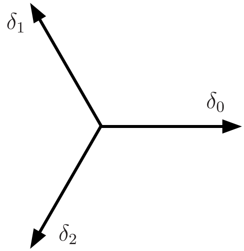
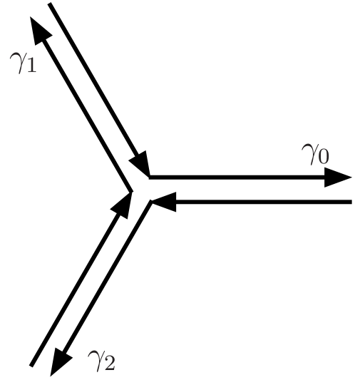
Figure 1: The integration cycles in a single variable Landau-Ginzburg model with worldsheet superpotential ${\cal W}=x^{3}$.

With reference to fig. 1, for $n=0,1,2\in\mathbb{Z}\bmod 3$ we let $\delta_{n}:=\omega^{n}[0,\infty)\subset{\mathbb{C}}\ni x$ be the three independent rays along which $x^{3}$ tends to real infinity, where $\omega=e^{2\pi{\rm i}/3}$. Then $\gamma_{n}:=\delta_{n}-\delta_{n+1}$ for $n=0,1,2$ span the lattice of cycles, subject to the one relation $\gamma_{0}+\gamma_{1}+\gamma_{2}=0$. For $l=1,2,\ldots$, we have

$$\int_{\delta_{n}}e^{-x^{3}}x^{l-1}dx=\omega^{n\cdot l}\cdot\frac{1}{3}\cdot\Gamma\bigl{(}\frac{l}{3}\bigr{)}$$ (A.3)

and therefore

$$w_{n,l}:=\int_{\gamma_{n}}e^{-x^{3}}x^{l-1}dx=\omega^{n\cdot l}(1-\omega^{l})\cdot\frac{1}{3}\cdot\Gamma\bigl{(}\frac{l}{3}\bigr{)}\,.$$ (A.4)

A.2 Taylor coefficients

Now, the deformation space of the $1^{9}$ LG model (2.1) is parametrized by local coordinates $\{t^{{\bf l}},{\bf l}=(l_{1},\ldots,l_{9})\in\{1,2\}^{9},\sum l_{i}=12\}$ via the worldsheet superpotential

$${\cal W}(t^{\bf l})=\sum_{i=1}^{9}x_{i}^{3}-\sum_{{\bf l}}t^{\bf l}{\bf x}^{{\bf l}-{\bf 1}}$$ (A.5)

where ${\bf x}^{\bf l}=\prod_{i}(x_{i})^{l_{i}}$ and ${\bf 1}=(1,1,1,1,1,1,1,1,1)$. Then, for ${\bf n}=(n_{1},\ldots,n_{9})\in\{0,1,2\}^{9}$, $\Gamma_{\bf n}=\times_{i}\gamma_{n_{i}}$ we can write the full moduli dependence of the period as

$$\begin{split}W_{\bf n}(t^{\bf l})&=\int_{\Gamma_{\bf n}}e^{-{\cal W}(t^{\bf l})}d^{9}x=\int_{\Gamma_{\bf n}}e^{-{\cal W}(0)}\sum_{K=0}^{\infty}\frac{1}{K!}\bigl{(}\textstyle\sum_{{\bf l}}t^{\bf l}{\bf x}^{{\bf l}-{\bf 1}}\bigr{)}^{K}d^{9}x\\ &=\int_{\Gamma_{\bf n}}e^{-{\cal W}(0)}\sum_{k_{\bf l}=0}^{\infty}\prod_{\bf l}\frac{\bigl{(}t^{\bf l}\bigr{)}^{k_{\bf l}}}{k_{\bf l}!}\bigl{(}{\bf x}^{{\bf l}-{\bf 1}}\bigr{)}^{k_{\bf l}}d^{9}x\\ &=\sum_{k_{\bf l}=0}^{\infty}\prod_{\bf l}\frac{\bigl{(}t^{\bf l}\bigr{)}^{k_{\bf l}}}{k_{\bf l}!}\prod_{i}\int_{\gamma_{n_{i}}}e^{-x_{i}^{3}}\bigl{(}x_{i}\bigr{)}^{\sum_{\bf l}k_{\bf l}(l_{i}-1)}dx_{i}\\ &=\sum_{k_{\bf l}}\prod_{\bf l}\frac{\bigl{(}t^{\bf l}\bigr{)}^{k_{\bf l}}}{k_{\bf l}!}\prod_{i}w_{n_{i},\sum_{\bf l}k_{\bf l}(l_{i}-1)+1}\end{split}$$ (A.6)

Equivalently, and perhaps more simply, we can evaluate the $r$-th multi-derivative as

$$\frac{\partial}{\partial t^{{\bf l}_{1}}}\frac{\partial}{\partial t^{{\bf l}_{2}}}\cdots\frac{\partial}{\partial t^{{\bf l}_{r}}}W_{\bf n}(0)=\int_{\Gamma_{\bf n}}e^{-{\cal W}(0)}\prod_{\alpha=1}^{r}{\bf x}^{{\bf l}_{\alpha}-{\bf 1}}d^{9}x\\ =\prod_{i}\int_{\gamma_{n_{i}}}e^{-x_{i}^{3}}\bigl{(}x_{i}\bigr{)}^{\sum_{\alpha=1}^{r}(l_{\alpha}^{i}-1)}dx_{i}=\prod_{i}w_{n_{i},\sum_{\alpha}l_{\alpha}^{i}-r+1}\\ =\frac{1}{3^{9}}\cdot\omega^{{\bf n}(\sum_{\alpha}{\bf l}_{\alpha}-(r-1){\bf 1})}\prod_{i}\bigl{(}1-\omega^{\sum_{\alpha}l_{\alpha}^{i}-(r-1)}\bigr{)}\cdot\Gamma\Bigl{(}\frac{\sum_{\alpha}l_{\alpha}^{i}-(r-1)}{3}\Bigr{)}$$ (A.7)

which is the expression we used in the main text in equation (2.23).

Appendix B The $G$-flux for an AdS solution

Here we give the explicit $G$-flux, discussed in subsection 5.3 above. It describes an AdS solution that has $N_{\rm flux}=12$ and thus satisfies the tadpole cancellation condition without D3-branes. The value of the axio-dilaton is $\tau=e^{\frac{2\pi{\rm i}}{3}}$ and all 64 complex scalars appear in the Hessian of the superpotential since it has maximal rank 64. The $G$-flux is given by

$$G =\frac{1}{18}\biggr{[}\left(15-{\rm i}\sqrt{3}\right)\left(-3\Omega_{1,1,1,1,1,1,1,1,1}+\Omega_{2,2,2,2,2,2,2,2,2}\right)$$

$${\rm i}\left(3{\rm i}+\sqrt{3}\right)\Omega_{1,1,1,1,1,1,2,2,2}-4\Omega_{1,2,1,1,2,1,1,1,2}+2\Omega_{1,1,2,1,2,1,1,1,2}$$

$$+{\rm i}\left(3{\rm i}+\sqrt{3}\right)\Omega_{1,1,1,1,1,2,1,2,2}+\left(3+{\rm i}\sqrt{3}\right)\Omega_{1,1,1,1,1,2,2,1,2}+{\rm i}\left(3{\rm i}+\sqrt{3}\right)\Omega_{1,1,1,1,1,2,2,2,1}$$

$$+\left(-5-{\rm i}\sqrt{3}\right)\Omega_{1,1,1,1,2,1,1,2,2}+\left(3+{\rm i}\sqrt{3}\right)\Omega_{1,1,1,1,2,1,2,2,1}-2{\rm i}\sqrt{3}\Omega_{1,1,1,1,2,2,1,1,2}$$

$$+\left(6+2{\rm i}\sqrt{3}\right)\Omega_{1,1,1,1,2,2,1,2,1}+2{\rm i}\sqrt{3}\Omega_{1,1,1,2,1,1,1,2,2}+2\Omega_{1,1,1,2,1,1,2,1,2}$$

$$+{\rm i}\left(3{\rm i}+\sqrt{3}\right)\Omega_{1,1,1,2,1,1,2,2,1}+{\rm i}\left(5{\rm i}+\sqrt{3}\right)\Omega_{1,1,1,2,1,2,1,2,1}+\left(1+{\rm i}\sqrt{3}\right)\Omega_{1,1,1,2,1,2,2,1,1}$$

$$+\left(2+2{\rm i}\sqrt{3}\right)\Omega_{1,1,1,2,2,1,1,1,2}+4\Omega_{1,1,1,2,2,1,1,2,1}+\left(-2-2{\rm i}\sqrt{3}\right)\Omega_{1,1,1,2,2,1,2,1,1}$$

$$+\left(-1-{\rm i}\sqrt{3}\right)\Omega_{1,1,1,2,2,2,1,1,1}+{\rm i}\left(3{\rm i}+\sqrt{3}\right)\Omega_{1,1,2,1,1,1,1,2,2}+\left(3+{\rm i}\sqrt{3}\right)\Omega_{1,1,2,1,1,1,2,1,2}$$

$$+{\rm i}\left(3{\rm i}+\sqrt{3}\right)\Omega_{1,1,2,1,1,1,2,2,1}+\left(3+{\rm i}\sqrt{3}\right)\Omega_{1,1,2,1,1,2,1,1,2}+{\rm i}\left(3{\rm i}+\sqrt{3}\right)\Omega_{1,1,2,1,1,2,1,2,1}$$

$$+\left(3+{\rm i}\sqrt{3}\right)\Omega_{1,1,2,1,1,2,2,1,1}+2{\rm i}\sqrt{3}\Omega_{1,1,2,1,2,1,1,2,1}+2\Omega_{1,1,2,1,2,1,2,1,1}$$

$$+\left(3+{\rm i}\sqrt{3}\right)\Omega_{1,1,2,1,2,2,1,1,1}+\left(1+{\rm i}\sqrt{3}\right)\Omega_{1,1,2,2,1,1,1,1,2}+{\rm i}\left({\rm i}+\sqrt{3}\right)\Omega_{1,1,2,2,1,1,1,2,1}$$

$$+\left(1+{\rm i}\sqrt{3}\right)\Omega_{1,1,2,2,1,1,2,1,1}+\left(1+{\rm i}\sqrt{3}\right)\Omega_{1,1,2,2,1,2,1,1,1}+\left(-5-{\rm i}\sqrt{3}\right)\Omega_{1,1,2,2,2,1,1,1,1}$$

$$-8\Omega_{1,2,1,1,1,1,1,2,2}+\left(2+2{\rm i}\sqrt{3}\right)\Omega_{1,2,1,1,1,1,2,1,2}+{\rm i}\left(3{\rm i}+\sqrt{3}\right)\Omega_{1,2,1,1,1,1,2,2,1}$$

$$+2{\rm i}\left({\rm i}+\sqrt{3}\right)\Omega_{1,2,1,1,1,2,1,2,1}+\left(1+3{\rm i}\sqrt{3}\right)\Omega_{1,2,1,1,1,2,2,1,1}+8\Omega_{1,2,1,1,2,1,1,2,1}$$

$$+\left(-3-{\rm i}\sqrt{3}\right)\Omega_{1,2,1,1,2,1,2,1,1}+2\Omega_{1,2,1,1,2,2,1,1,1}+\left(5+3{\rm i}\sqrt{3}\right)\Omega_{1,2,1,2,1,1,1,1,2}$$

$$+\left(-1-{\rm i}\sqrt{3}\right)\Omega_{1,2,1,2,1,1,2,1,1}-4\Omega_{1,2,1,2,1,2,1,1,1}+\left(4+4{\rm i}\sqrt{3}\right)\Omega_{1,2,1,2,2,1,1,1,1}+$$

$$\left(3+3{\rm i}\sqrt{3}\right)\Omega_{1,2,2,1,1,1,1,1,2}+2{\rm i}\left(2{\rm i}+\sqrt{3}\right)\Omega_{1,2,2,1,1,1,1,2,1}+\left(3+3{\rm i}\sqrt{3}\right)\Omega_{1,2,2,1,1,1,2,1,1}$$

$$+\left(4+4{\rm i}\sqrt{3}\right)\Omega_{1,2,2,1,1,2,1,1,1}+2{\rm i}\left(2{\rm i}+\sqrt{3}\right)\Omega_{1,2,2,1,2,1,1,1,1}+{\rm i}\left(3{\rm i}+\sqrt{3}\right)\Omega_{1,2,2,2,1,1,1,1,1}$$

$$-8\Omega_{2,1,1,1,1,1,1,2,2}+\left(2+2{\rm i}\sqrt{3}\right)\Omega_{2,1,1,1,1,1,2,1,2}+{\rm i}\left(3{\rm i}+\sqrt{3}\right)\Omega_{2,1,1,1,1,1,2,2,1}$$

$$+2{\rm i}\left({\rm i}+\sqrt{3}\right)\Omega_{2,1,1,1,1,2,1,2,1}+\left(1+3{\rm i}\sqrt{3}\right)\Omega_{2,1,1,1,1,2,2,1,1}-4\Omega_{2,1,1,1,2,1,1,1,2}$$

$$+\left(-3-{\rm i}\sqrt{3}\right)\Omega_{2,1,1,1,2,1,2,1,1}+2\Omega_{2,1,1,1,2,2,1,1,1}+\left(5+3{\rm i}\sqrt{3}\right)\Omega_{2,1,1,2,1,1,1,1,2}$$

$$+4\Omega_{2,1,1,2,1,1,1,2,1}+\left(-1-{\rm i}\sqrt{3}\right)\Omega_{2,1,1,2,1,1,2,1,1}-4\Omega_{2,1,1,2,1,2,1,1,1}$$ (B.1)

$$+\left(3+3{\rm i}\sqrt{3}\right)\Omega_{2,1,2,1,1,1,1,1,2}+2{\rm i}\left(2{\rm i}+\sqrt{3}\right)\Omega_{2,1,2,1,1,1,1,2,1}+\left(3+3{\rm i}\sqrt{3}\right)\Omega_{2,1,2,1,1,1,2,1,1}$$ (B.2)

$$+\left(4+4{\rm i}\sqrt{3}\right)\Omega_{2,1,2,1,1,2,1,1,1}+2{\rm i}\left(2{\rm i}+\sqrt{3}\right)\Omega_{2,1,2,1,2,1,1,1,1}+{\rm i}\left(3{\rm i}+\sqrt{3}\right)\Omega_{2,1,2,2,1,1,1,1,1}$$

$$+4\Omega_{1,2,1,2,1,1,1,2,1}+8\Omega_{2,1,1,1,2,1,1,2,1}+\left(4+4{\rm i}\sqrt{3}\right)\Omega_{2,1,1,2,2,1,1,1,1}$$

$$+{\rm i}\left({\rm i}+\sqrt{3}\right)\Omega_{2,2,1,1,1,1,1,1,2}+8\Omega_{2,2,1,1,1,1,1,2,1}-2\Omega_{2,2,1,1,1,1,2,1,1}$$

$$+{\rm i}\left({\rm i}+\sqrt{3}\right)\Omega_{2,2,1,1,1,2,1,1,1}+2{\rm i}\sqrt{3}\Omega_{2,2,1,1,2,1,1,1,1}$$

$$+2\left(5+2{\rm i}\sqrt{3}\right)\Omega_{2,2,1,2,1,1,1,1,1}+\left(-2+4{\rm i}\sqrt{3}\right)\Omega_{2,2,2,1,1,1,1,1,1}\biggr{]}\,.$$ (B.3)

References

- [1] S.B. Giddings, S. Kachru and J. Polchinski, Hierarchies from fluxes in string compactifications, Phys. Rev. D 66 (2002) 106006 [hep-th/0105097].
- [2] A. Giryavets, S. Kachru, P.K. Tripathy and S.P. Trivedi, Flux compactifications on Calabi-Yau threefolds, JHEP 04 (2004) 003 [hep-th/0312104].
- [3] F. Denef, M.R. Douglas and B. Florea, Building a better racetrack, JHEP 06 (2004) 034 [hep-th/0404257].
- [4] F. Denef, M.R. Douglas, B. Florea, A. Grassi and S. Kachru, Fixing all moduli in a simple f-theory compactification, Adv. Theor. Math. Phys. 9 (2005) 861 [hep-th/0503124].
- [5] A. Collinucci, F. Denef and M. Esole, D-brane Deconstructions in IIB Orientifolds, JHEP 02 (2009) 005 [0805.1573].
- [6] I. Bena, J. Blåbäck, M. Graña and S. Lüst, The tadpole problem, JHEP 11 (2021) 223 [2010.10519].
- [7] I. Bena, J. Blåbäck, M. Graña and S. Lüst, Algorithmically Solving the Tadpole Problem, Adv. Appl. Clifford Algebras 32 (2022) 7 [2103.03250].
- [8] I. Bena, C. Brodie and M. Graña, D7 moduli stabilization: the tadpole menace, JHEP 01 (2022) 138 [2112.00013].
- [9] E. Palti, The Swampland: Introduction and Review, Fortsch. Phys. 67 (2019) 1900037 [1903.06239].
- [10] M. van Beest, J. Calderón-Infante, D. Mirfendereski and I. Valenzuela, Lectures on the Swampland Program in String Compactifications, 2102.01111.
- [11] P. Betzler and E. Plauschinn, Type IIB flux vacua and tadpole cancellation, Fortsch. Phys. 67 (2019) 1900065 [1905.08823].
- [12] E. Plauschinn, The tadpole conjecture at large complex-structure, JHEP 02 (2022) 206 [2109.00029].
- [13] M. Graña, T.W. Grimm, D. van de Heisteeg, A. Herraez and E. Plauschinn, The tadpole conjecture in asymptotic limits, JHEP 08 (2022) 237 [2204.05331].
- [14] K. Tsagkaris and E. Plauschinn, Moduli stabilization in type IIB orientifolds at , 2207.13721.
- [15] F. Marchesano, D. Prieto and M. Wiesner, F-theory flux vacua at large complex structure, JHEP 08 (2021) 077 [2105.09326].
- [16] S. Lüst, Large complex structure flux vacua of IIB and the Tadpole Conjecture, 2109.05033.
- [17] A.P. Braun and R. Valandro, flux, algebraic cycles and complex structure moduli stabilization, JHEP 01 (2021) 207 [2009.11873].
- [18] K. Becker, M. Becker, C. Vafa and J. Walcher, Moduli Stabilization in Non-Geometric Backgrounds, Nucl. Phys. B 770 (2007) 1 [hep-th/0611001].
- [19] K. Becker, M. Becker and J. Walcher, Runaway in the Landscape, Phys. Rev. D 76 (2007) 106002 [0706.0514].
- [20] K. Ishiguro and H. Otsuka, Sharpening the boundaries between flux landscape and swampland by tadpole charge, JHEP 12 (2021) 017 [2104.15030].
- [21] J. Bardzell, E. Gonzalo, M. Rajaguru, D. Smith and T. Wrase, Type IIB flux compactifications with h1,1 = 0, JHEP 06 (2022) 166 [2203.15818].
- [22] B.S. Acharya and M.R. Douglas, A Finite landscape?, hep-th/0606212.
- [23] C. Vafa, The String landscape and the swampland, hep-th/0509212.
- [24] O. DeWolfe, A. Giryavets, S. Kachru and W. Taylor, Type IIA moduli stabilization, JHEP 07 (2005) 066 [hep-th/0505160].
- [25] P.G. Camara, A. Font and L.E. Ibanez, Fluxes, moduli fixing and MSSM-like vacua in a simple IIA orientifold, JHEP 09 (2005) 013 [hep-th/0506066].
- [26] K. Hori and J. Walcher, D-brane categories for orientifolds—the landau-ginzburg case, Journal of High Energy Physics 2008 (2008) 030.
- [27] K. Dasgupta, G. Rajesh and S. Sethi, M theory, orientifolds and G - flux, JHEP 08 (1999) 023 [hep-th/9908088].
- [28] S. Gukov, C. Vafa and E. Witten, CFT’s from Calabi-Yau four folds, Nucl. Phys. B 584 (2000) 69 [hep-th/9906070].
- [29] M. Kim, D-instanton superpotential in string theory, JHEP 03 (2022) 054 [2201.04634].
- [30] M. Marino, R. Minasian, G.W. Moore and A. Strominger, Nonlinear instantons from supersymmetric p-branes, JHEP 01 (2000) 005 [hep-th/9911206].
- [31] T.W. Grimm and J. Louis, The Effective action of N = 1 Calabi-Yau orientifolds, Nucl. Phys. B 699 (2004) 387 [hep-th/0403067].
- [32] T.W. Grimm and J. Louis, The Effective action of type IIA Calabi-Yau orientifolds, Nucl. Phys. B 718 (2005) 153 [hep-th/0412277].
- [33] P. Candelas and X. de la Ossa, Moduli Space of Calabi-Yau Manifolds, Nucl. Phys. B 355 (1991) 455.
- [34] F. Denef and M.R. Douglas, Distributions of flux vacua, Journal of High Energy Physics 2004 (2004) 072.
- [35] F. Denef and M.R. Douglas, Computational complexity of the landscape: Part i, Annals of Physics 322 (2007) 1096.
- [36] Y. Hamada, M. Montero, C. Vafa and I. Valenzuela, Finiteness and the swampland, J. Phys. A 55 (2022) 224005 [2111.00015].
- [37] P. Breitenlohner and D.Z. Freedman, Positive Energy in anti-De Sitter Backgrounds and Gauged Extended Supergravity, Phys. Lett. B 115 (1982) 197.
- [38] A. Hanany and A. Zaffaroni, Chiral symmetry from type IIA branes, Nucl. Phys. B 509 (1998) 145 [hep-th/9706047].
- [39] I. Brunner and A. Karch, Branes at orbifolds versus Hanany Witten in six-dimensions, JHEP 03 (1998) 003 [hep-th/9712143].
- [40] C.-h. Ahn, K. Oh and R. Tatar, Orbifolds of AdS(7) x S**4 and six-dimensional (0,1) SCFT, Phys. Lett. B 442 (1998) 109 [hep-th/9804093].
- [41] A. Hanany and A. Zaffaroni, Branes and six-dimensional supersymmetric theories, Nucl. Phys. B 529 (1998) 180 [hep-th/9712145].
- [42] S. Ferrara, A. Kehagias, H. Partouche and A. Zaffaroni, Membranes and five-branes with lower supersymmetry and their AdS supergravity duals, Phys. Lett. B 431 (1998) 42 [hep-th/9803109].
- [43] D. Lüst, E. Palti and C. Vafa, AdS and the Swampland, Phys. Lett. B 797 (2019) 134867 [1906.05225].
- [44] G. Veneziano, Large N bounds on, and compositeness limit of, gauge and gravitational interactions, JHEP 06 (2002) 051 [hep-th/0110129].
- [45] N. Arkani-Hamed, S. Dimopoulos and S. Kachru, Predictive landscapes and new physics at a TeV, hep-th/0501082.
- [46] G. Dvali, Black Holes and Large N Species Solution to the Hierarchy Problem, Fortsch. Phys. 58 (2010) 528 [0706.2050].
- [47] G. Dvali and M. Redi, Black Hole Bound on the Number of Species and Quantum Gravity at LHC, Phys. Rev. D 77 (2008) 045027 [0710.4344].
- [48] P. Berglund, P. Candelas, X. de la Ossa, A. Font, T. Hübsch, D. Jančić et al., Periods for Calabi-Yau and Landau-Ginzburg vacua, Nuclear Physics B 419 (1994) 352.