Joint Communication and Sensing in RIS-enabled mmWave Networks

Abstract

Empowering cellular networks with augmented sensing capabilities is a key research area in sixth generation (6G) communication systems. Recently, we have witnessed a plethora of efforts to devise solutions that integrate sensing capabilities into communication systems, i.e., joint communication and sensing (JCAS). However, most prior works do not consider the impact of reconfigurable intelligent surfaces (RISs) on JCAS systems at millimeter-wave (mmWave) bands. Given that RISs are expected to become an integral part of future cellular systems, it is important to investigate their potential in cellular networks beyond communication goals. To comply with the waveform utilized in current cellular systems, this paper studies mmWave orthogonal frequency-division multiplexing (OFDM) JCAS systems in the presence of RISs. Specifically, we jointly design the hybrid beamforming and RIS phase shifts to guarantee the sensing functionalities via minimizing the beampattern mean square error at RIS, subject to signal-to-interference-plus-noise (SINR) and power constraints. The non-convexity of the investigated problem poses a challenge which we address by proposing a solution based on the penalty method and manifold-based alternating direction method of multipliers (ADMM). Simulation results demonstrate that both sensing and communication capabilities improve when the RIS is adequately designed. In addition, we discuss the tradeoff between sensing and communication.

I Introduction

Joint communication and sensing (JCAS) is one of the core research areas in the sixth generation (6G) communication systems. By integrating sensing and communication into one physical unity, JCAS adds a new dimension to network intelligence allowing users and operators to simultaneously communicate and obtain/sense information from their surrounding environment [1]. This opens up new possibilities for emerging use-cases involving autonomous or assisted navigation and smart home monitoring. Meanwhile, JCAS systems are expected to be deployed in the millimeter-wave (mmWave) bands which provide the benefit of larger bandwidth to achieve higher throughput and sensing resolution. However, integrating sensing and communication is a challenging task, in particular, at mmWave frequencies where signals are prone to high attenuation and blockage due to the short wavelength and high path loss [2].

To tackle these problems, base stations (BSs) and users rely on highly directional beamforming, which requires efficient beamforming in JCAS scenarios not only towards the communication end-points but also the sensed targets. In mmWave JCAS systems, digital beamforming is difficult to realize due to the high cost of having one dedicated radio frequency (RF) chain for each antenna element, which motivates the exploitation of hybrid beamforming. Furthermore, to circumvent the blockages met at mmWave frequencies, reconfigurable intelligent surfaces (RISs) are a promising solution, which are expected to be deployed massively in 6G communication systems. RISs are planar electromagnetic surfaces consisting of a large number of controllable reflecting elements. Depending on the design, RISs can be controlled to alter the phase and amplitude of the incident signal without complex decoding, encoding, and radio-frequency processing operations. This makes RISs a scalable solution to circumvent the issue of susceptibility to blockages in a cost-effective manner. Therefore, we consider introducing the RIS into JCAS networks, which makes the system design of JCAS become even more challenging. Particularly, the beamforming design in such scenarios should simultaneously consider the mobile users for communication, the targets for sensing, and the phase configuration of RIS.

I-A Prior Works

To date, the majority of existing works focused on either JCAS [3, 4, 5, 6, 7, 8, 9, 10, 11, 2, 12, 13, 14, 15, 16, 17, 18] or RISs [19, 20, 21, 22, 23, 24, 25, 26, 27, 28]. Hence, we first provide an overview of the state of the art on JCAS and RISs respectively, and then review the works that address JCAS in the presence of RISs.

JCAS. The existing works in JCAS mostly focused on the waveform design [3, 4, 5, 6], performance tradeoff optimization [7, 8, 9], communication-assisted sensing [10, 11], and sensing-assisted communication [2, 12]. In recent years, we have observed more works on the design of JCAS at mmWave bands [2, 12, 13, 14, 15, 16, 17, 18]. Specifically, in [13, 14, 15], the authors designed hybrid beamformers by formulating a tradeoff problem between communication and sensing. Besides, the works in [16, 17] designed the hybrid beamforming for multi-carrier JCAS systems. The works in [2, 12, 18] investigated beam training, tracking, and prediction in JCAS systems at mmWave bands.

RIS. Intelligent surfaces have been extensively studied from a communication perspective in recent years [19] for different design goals including sum-rate maximization [20], power minimization [21], and energy efficiency maximization [22], and for various scenarios including non-orthogonal multiple access [23], mobile edge computing [24], and simultaneous wireless information and power transfer [25]. A few works have also exploited RISs for sensing but mainly focused on detection and estimation aspects, such as improving target detection probability [26], target parameters estimation [27], and human gesture recognition [28]. All these foregoing applications of RIS in either communication systems or sensing systems demonstrate the potential of exploiting RIS in JCAS system.

RIS-assisted JCAS. The number of works investigating JCAS in the presence of RISs [29, 30, 31, 32, 33, 34, 35, 36, 37, 38, 39, 40, 41, 42, 43, 44, 45, 46, 47, 48, 49, 50, 51, 52] is significantly less than the aforementioned two categories. The works [29, 30, 31, 32, 33, 34, 35, 36, 37] considered JCAS-enabled base stations (BSs) but the RIS usage was either limited to sensing/localization [29, 30, 31, 32] or communication [33, 34, 35, 36, 37]. The authors of [38, 39, 40] designed JCAS systems leveraging RISs for scenarios with a single user and a single target. Furthermore, the authors of [41, 42, 43, 44, 45, 46] investigated RIS-assisted JCAS systems for one single target and multiple users using different sensing metrics. To be specific, subject to signal-to-interference-plus-noise-ratio (SINR) or sum rate constraint for communication users, the sensing performance was optimized with different goals, namely radar SINR maximization in [41, 42], Cramér-Rao lower bound minimization in [43, 44], beampattern gain towards targets maximization [45, 46]. Single-user and multi-target systems were studied in [47], where the minimum beampattern gain for each of the targets was maximized subject to the signal-to-noise-ratio (SNR) requirement for one single user. As a step forward, multi-target and multi-user systems were investigated in [48, 49, 50, 51, 52]. Specifically, the authors of [48, 49, 50] maximized the minimum target illumination power or minimized the beampattern design mean square error (MSE) to guarantee the sensing performance while satisfying the SINR constraint for users. The work [51] investigated the tradeoff between the sensing mutual information of targets and the SINR of users. The work [52] jointly designed the beamforming and phase shifts in the terahertz band to maximize the sum rate of communication users by satisfying a beampattern MSE constraint.

TABLE I: RIS-assisted JCAS Related Works.

Ref.	System		Spectrum	OFDM	Beamforming	RIS
	Users	Targets				Communication	Sensing
[29]	✗	Single	Sub-6 GHz	✗	✗	✗	✓
[30]	✗	Single	Sub-6 GHz	✗	Digital beamforming	✗	✓
[31, 32]	✗	Multiple	Sub-6 GHz	✗	Digital beamforming	✗	✓
[33, 34]	Multiple	Multiple	Sub-6 GHz	✗	✗	✓	✗
[35, 36]	Multiple	Multiple	Sub-6 GHz	✗	Digital beamforming	✓	✗
[37]	Multiple	Multiple	mmWave	✗	Digital beamforming	✓	✗
[38]	Single	Single	mmWave	✗	✗	✓	✓
[39, 40]	Single	Single	Sub-6 GHz	✗	Digital beamforming	✓	✓
[41]	Multiple	Single	Sub-6 GHz	✓	Digital beamforming	✓	✓
[42, 43, 44, 45, 46]	Multiple	Single	Sub-6 GHz	✗	Digital beamforming	✓	✓
[47]	Single	Multiple	Sub-6 GHz	✗	Digital beamforming	✓	✓
[48, 49, 51, 50]	Multiple	Multiple	Sub-6 GHz	✗	Digital beamforming	✓	✓
[52]	Multiple	Multiple	Terahertz	✗	Digital beamforming	✓	✓
This paper	Multiple	Multiple	mmWave	✓	Hybrid beamforming	✓	✓

However, the beamforming solutions in the aforementioned RIS-based JCAS networks only apply to fully-digital beamforming, which is difficult to realize at higher frequencies. Table I summarizes the state of the art in RIS-assisted JCAS research. We highlight that none of the aforementioned works has considered the RIS-assisted JCAS design in mmWave orthogonal frequency-division multiplexing (OFDM) systems, which requires the joint optimization of the RIS phase shifts and hybrid beamforming, while taking into account the multi-carrier nature of the modern wireless communication system. Next, we discuss our motivation and contributions.

I-B Contributions

In this article, we investigate RIS-assisted OFDM JCAS systems in mmWave cellular networks. Aligned with 5G new radio (NR) specifications, we adopt OFDM as the physical waveform of the system and consider multiple targets and users which experience different channel conditions on each sub-carrier [53]. To improve the performance of communication and sensing, we jointly design the hybrid beamforming and RIS phase shifts, thus guaranteeing $(i)$ the communication for mobile users and $(ii)$ the sensing of targets. To realize the aforementioned goals, we formulate an optimization problem that proves to be non-convex, in particular, due to variable coupling, non-convex objective function and SINR constraints, and constant-modulus constraints that are inherent to the RIS elements and hybrid beamforming. Therefore, we propose a manifold-based alternating direction method of multipliers (ADMM) algorithm which is capable of coping with the complex structure of the formulated problem. In the following, we summarize our contributions in more detail.

• To the best of our knowledge, this is the first effort toward modeling an OFDM JCAS cellular system at mmWave bands in the presence of RISs. To guarantee the sensing performance, we minimize the difference between the designed and reference beampatterns at the RIS across all sub-carriers. In particular, the reference beampattern is designed to have main lobes in the directions of targets. As constraints, we incorporate SINR requirements for each user and each sub-carrier in order to guarantee the communication performance. In addition, we consider the transmit power constraint and constant-modulus phase shifts due to the hybrid beamforming and RIS.

• To solve the non-convex problem, we propose a scheme based on the penalty method and the ADMM algorithm. Specifically, we first introduce an auxiliary variable to decouple the RF beamformer and baseband beamformer. Then, we use the penalty method to overcome the non-convex SINR constraints by integrating them into the objective function. To tackle the newly transformed problem, we adopt a manifold-based ADMM framework, where each variable is optimized in an alternating and iterative manner until convergence.

• We evaluate our proposed scheme via extensive simulations under different parameter settings. Specifically, we assess its performance by analyzing the convergence, the sensing performance, and the communication performance. The sensing performance is evaluated via the beampattern MSE between the designed and reference beampatterns at the RIS, and the peak-side-lobe-ratio (PSLR) produced by the generated beampattern. The communication performance is evaluated via the feasibility ratio of SINR values above the predefined threshold. Furthermore, three benchmark schemes are included for comparison, namely fully-digital beamforming with RIS, fully-digital beamforming with random RIS phase shifts, and hybrid beamforming with random RIS phase shifts. The results show that our proposed scheme improves both sensing and communication performances with the assistance of RIS. The tradeoff between sensing and communication is also illustrated via comparing the SINR feasibility ratio and average SINR versus the beampattern MSE.

I-C Organization and Notation

The remainder of this paper is organized as follows: Section II introduces the system model of the RIS-assisted mmWave OFDM JCAS system followed by the problem formulation. Section III presents the proposed solution and its computational complexity analysis. We provide simulation results and discussion in Section V. Finally, conclusions are summarized in Section VI.

In this paper, bold-face uppercase and lowercase, ${\bf{A}}$ and ${\bf{a}}$, represent matrices and vectors, respectively. $\mathbb{E}\left\{\cdot\right\}$, ${\rm{tr}}\left(\cdot\right)$, and ${\mathcal{O}}\left(\cdot\right)$ stand for the expectation, the trace of a square matrix, and the computational complexity order. ${\left(\cdot\right)^{\rm{T}}}$ and ${\left(\cdot\right)^{\rm{H}}}$ denote the transpose and the Hermitian transpose of a matrix or vector. $\left|\cdot\right|$ and ${\left\|\cdot\right\|_{\rm{F}}}$ represent the absolute value of a scalar and the Frobenius norm of a matrix, respectively. The symbols $\otimes$, $\odot$, $\left\langle{\cdot,\cdot}\right\rangle$ represent the Kronecker product, the Hadamard product, and the Euclidean inner product, respectively. ${\nabla}$ denotes the Euclidean gradient. ${\rm{blkdiag}}\left(\cdot\right)$ and ${\rm{diag}}\left(\cdot\right)$ are functions to form a block diagonal or diagonal matrix with the elements in $\left(\cdot\right)$, respectively. ${\mathbb{C}}$ and ${\mathbb{R}}$ denote the complex and real numbers, respectively.

II System Model and Problem Formulation

We consider an OFDM JCAS system operating at mmWave frequencies, where an RIS is deployed to assist both communication and sensing, as shown in Fig. 1. The signals transmitted from the BS arrive at the user equipments (UEs) by direct transmission and indirect reflection via the RIS. For sensing, we consider the situation where the direct links between the BS and the targets are blocked. Thus, the RIS is deployed to circumvent the blockage and enable sensing. The BS is equipped with ${{N}_{t}}$ antennas, which are spaced by half wavelength thus forming a uniform linear array (ULA). In addition, the BS has a small number of RF chains which is denoted by $N_{RF}$, such that $N_{RF}<<{{N}_{t}}$. The BS serves $K$ single-antenna UEs and senses $M$ targets, simultaneously. The number of sub-carriers is denoted as $N_{c}$. The interval between adjacent sub-carriers is $\Delta f$. The RIS is configured with $R$ reflecting elements and modeled as a ULA structure. Regarding the reflected path from the RIS, let ${{\theta}_{r}}\in[0,2\pi)$ denote the phase shift imposed by the $r$-th reflection element on the incident signals and $\Theta={\rm{diag}}({{e}^{j{{\theta}_{1}}}},\cdots,{{e}^{j{{\theta}_{R}}}})$ group the phase shifts of all RIS elements. Due to the high path loss at mmWave band, it is assumed that the transmission signals reflected two or more times by the RIS are negligible and thus ignored [54].

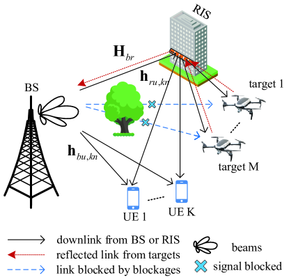
Figure 1: Overview of the RIS-assisted JCAS system at mmWave frequency.

II-A Transmission Signals and Hybrid Beamforming

Let ${\bf{X}}={[{\bf{X}}_{1}^{\rm{T}},...,{\bf{X}}_{n}^{\rm{T}},...,{\bf{X}}_{{N_{c}}}^{\rm{T}}]^{\rm{T}}}\in{\mathbb{C}^{{N_{c}}K\times L}}$ denote the transmit symbols from the BS to all the $K$ UEs on all the $N_{c}$ sub-carriers, where ${{\bf{X}}_{n}}={[{{\bf{x}}_{1,n}},...,{{\bf{x}}_{k,n}},...,{{\bf{x}}_{K,n}}]^{\rm{T}}}\in{\mathbb{C}^{K\times L}}$ stands for the transmit symbols for all the $K$ UEs on the sub-carrier $n\in{\mathcal{N}_{c}}$. Besides, $L$ represents the length of symbols. ${{\bf{x}}_{k,n}}\in{\mathbb{C}^{L\times 1}}$ refers to the data for the UE $k$ on the sub-carrier $n$, satisfying $\mathbb{E}{\{{{\bf{x}}_{k,n}}{\bf{x}}_{k,n}^{\rm{H}}\}}={{\bf{I}}_{L}}$.

Hybrid beamforming consists of digital beamforming (a.k.a. baseband precoding) and analog beamforming (a.k.a. RF analog processing). The baseband digital beamforming is sub-carrier dependent whereas RF analog beamforming is identical for all the sub-carriers [55]. The transmit symbols are first digitally processed by the precoding matrix ${{\bf{W}}^{BB}}$ in the frequency domain as

$${{\bf{X}}^{BB}}={{\bf{W}}^{BB}}{\bf{X}}={[{\left({{\bf{X}}_{1}^{BB}}\right)^{\rm{T}}},...,{\left({{\bf{X}}_{{N_{c}}}^{BB}}\right)^{\rm{T}}}]^{\rm{T}}}\in{\mathbb{C}}{{}^{{N_{c}}{N_{RF}}\times L}},$$ (1)

where ${{\bf{W}}^{BB}}={\rm{blkdiag}}({\bf{W}}_{1}^{BB},...,{\bf{W}}_{n}^{BB},...,{\bf{W}}_{{N_{c}}}^{BB})\in{\mathbb{C}^{{N_{c}}{N_{RF}}\times{N_{c}}K}}$ collects the precoding matrices for all the $K$ UEs on all the $N_{c}$ sub-carriers, ${\bf{W}}_{n}^{BB}=[{\bf{w}}_{1,n}^{BB},...,{\bf{w}}_{k,n}^{BB},...,{\bf{w}}_{K,n}^{BB}]\in{\mathbb{C}^{{N_{RF}}\times K}}$ represents the baseband precoding matrix for all the $K$ UEs on the sub-carrier $n$, and ${\bf{w}}_{k,n}^{BB}\in{\mathbb{C}^{{N_{RF}}\times 1}}$ is the baseband precoding vector for the UE $k$ on the sub-carrier $n$. Besides, ${\bf{X}}_{n}^{BB}={\bf{W}}_{n}^{BB}{{\bf{X}}_{n}}\in{\mathbb{C}^{{N_{RF}}\times L}}$ is the precoded signal after digital beamforming for all the $K$ UEs on the sub-carrier $n$.

Then, the inverse discrete Fourier transform (IDFT) operation is applied to ${\bf{X}}^{BB}$ thus yielding

$${{{\bf{X}}^{ID}}=({{\bf{F}}^{\rm{H}}}\otimes{{\bf{I}}_{{N_{RF}}}}){{\bf{W}}^{BB}}{\bf{X}}\in{\mathbb{C}^{{N_{c}}{N_{RF}}\times L}}={{[{{\left({{\bf{X}}_{1}^{ID}}\right)}^{\rm{T}}},...,{{\left({{\bf{X}}_{{N_{c}}}^{ID}}\right)}^{\rm{T}}}]}^{\rm{T}}}}\in{\mathbb{C}}{{}^{{N_{c}}{N_{RF}}\times L}},$$ (2)

where ${\bf{F}}\in{\mathbb{C}^{{N_{c}}\times{N_{c}}}}$ is the discrete Fourier transform (DFT) matrix. The $(n,n^{\prime})$-th element of ${\bf{F}}$ $(n\in{\mathcal{N}_{c}},n^{\prime}\in{\mathcal{N}_{c}})$ is calculated as follows

$${F_{n,n^{\prime}}}=\frac{1}{{\sqrt{{N_{c}}}}}{e^{-\frac{{j2\pi}}{{{N_{c}}}}(n-1)(n^{\prime}-1)}}.$$ (3)

Therefore, $({{\bf{F}}^{\rm{H}}}\otimes{{\bf{I}}_{{N_{RF}}}})\in{\mathbb{C}^{N_{c}{N_{RF}}\times N_{c}{N_{RF}}}}$ in (2) corresponds to a $N_{c}$-point IDFT for all the $N_{RF}$ RF chains. In addition, ${\bf{X}}_{n}^{ID}=({\bf{f}}_{n}^{\rm{H}}\otimes{{\bf{I}}_{{N_{RF}}}}){\bf{W}}^{BB}{\bf{X}}\in{\mathbb{C}^{{N_{RF}}\times L}}$ in (2) is the transmitted signal after the IDFT operation for all the $N_{RF}$ RF chains on the sub-carrier $n$, where ${{\bf{f}}_{n}}\in{\mathbb{C}^{{N_{c}}\times 1}}$ is the $n$-th column of ${\bf{F}}$, corresponding to the DFT operation on the sub-carrier $n$.

Within the OFDM structure, the cyclic prefix is then added at the beginning of each OFDM symbol to deal with inter-symbol interference. Afterwards, the signals are up-converted, and RF analog beamforming is performed with the RF precoder ${{\bf{W}}^{RF}}={\rm{blkdiag}}({\bf{W}}_{1}^{RF},...,{\bf{W}}_{{N_{c}}}^{RF})\in{\mathbb{C}^{N_{c}N_{t}\times N_{c}N_{RF}}}$ in the time domain. Since the RF precoder is the same for all sub-carriers, we use ${{{{\bf{\tilde{W}}}}^{RF}}}$ to denote the RF precoder on each sub-carrier, such that ${\bf{W}}_{1}^{RF}={\bf{W}}_{2}^{RF}=\cdots={\bf{W}}_{{N_{c}}}^{RF}={{{\bf{\tilde{W}}}}^{RF}}\in{\mathbb{C}^{{N_{t}}\times{N_{RF}}}}$. Therefore, the transmitted signal of all the $K$ UEs on all the $N_{c}$ sub-carriers after RF analog beamforming can be expressed as follows

$${{\bf{X}}^{RF}}={{\bf{W}}^{RF}}({{\bf{F}}^{\rm{H}}}\otimes{{\bf{I}}_{{N_{RF}}}}){{\bf{W}}^{BB}}{\bf{X}}\in{\mathbb{C}^{{N_{c}}{N_{t}}\times L}}={[{\left({{\bf{X}}_{1}^{RF}}\right)^{\rm{T}}},...,{\left({{\bf{X}}_{{N_{c}}}^{RF}}\right)^{\rm{T}}}]^{\rm{T}}}\in{\mathbb{C}}{{}^{{N_{c}}{N_{t}}\times L}},$$ (4)

where ${\bf{X}}_{n}^{RF}={{{\bf{\tilde{W}}}}^{RF}}({\bf{f}}_{n}^{\rm{H}}\otimes{{\bf{I}}_{{N_{RF}}}}){\bf{W}}^{BB}{\bf{X}}\in{\mathbb{C}^{N_{t}\times L}}$ is the signal for all the $K$ UEs on the $n$-th sub-carrier after analog beamforming.

II-B Communication and Channel Model

The signal ${\bf{X}}^{RF}$ is transmitted from the BS to $K$ UEs through the direct link and the indirect link reflected by the RIS. The received signals can be expressed as follows

$${{\bf{Y}}_{c}}=({\bf{H}}_{bu}^{\rm{H}}+{\bf{H}}_{ru}^{\rm{H}}\hat{\Theta}{\bf{H}}_{br}^{\rm{H}}){{\bf{W}}^{RF}}({{\bf{F}}^{\rm{H}}}\otimes{{\bf{I}}_{{N_{RF}}}}){{\bf{W}}^{BB}}{\bf{X}}+{{\bf{N}}_{c}},$$ (5)

where ${{\bf{N}}_{c}}$ is the complex Gaussian noise during the transmission with zero mean and variance $\sigma_{c}^{2}$. $\hat{\Theta}={\rm{blkdiag}}(\Theta,...,\Theta)\in{{\mathbb{C}}^{{{N}_{c}R}\times{N}_{c}R}}$ is $N_{c}$ repetitions of $\Theta$ to match the matrix multiplication. ${{\bf{H}}_{bu}}={\rm{blkdiag}}({{\bf{H}}_{bu,1}},...,{{\bf{H}}_{bu,n}},...,{{\bf{H}}_{bu,{N_{c}}}})\in{{\mathbb{C}}^{{{N}_{c}{N}_{t}}\times{N}_{c}K}}$, ${{\bf{H}}_{br}}={\rm{blkdiag}}({{\bf{H}}_{br,1}},...,{{\bf{H}}_{br,n}},...,$ ${{\bf{H}}_{br,{N_{c}}}})\in{{\mathbb{C}}^{{{N}_{c}{N}_{t}}\times{{N}_{c}R}}}$ and ${{\bf{H}}_{ru}}={\rm{blkdiag}}({{\bf{H}}_{ru,1}},...,{{\bf{H}}_{ru,n}},...,{{\bf{H}}_{ru,{N_{c}}}})\in{{\mathbb{C}}^{{{N}_{c}R}\times{N}_{c}K}}$ are the channels on all the $N_{c}$ sub-carriers from the BS to $K$ UEs, from the BS to the RIS, and from the RIS to $K$ UEs, respectively.

For each sub-carrier $n$, ${{\bf{H}}_{bu,n}}=[{{\bf{h}}_{bu,1n}},...,{{\bf{h}}_{bu,kn}},...,{{\bf{h}}_{bu,Kn}}]\in{{\mathbb{C}}^{{{N}_{t}}\times K}}$ is the channel from the BS to $K$ UEs, where ${{\bf{h}}_{bu,kn}}\in{{\mathbb{C}}^{{{N}_{t}}\times 1}}$ is the channel from the BS to the UE $k$ on the sub-carrier $n$, modelled as the extended Saleh-Valenzuela model [53] given by

$${{\bf{h}}_{bu,kn}}=\sqrt{\frac{{{N_{t}}}}{{{N_{cl}}{N_{p}}}}}\sum\limits_{c}^{{N_{cl}}}{\sum\limits_{p}^{{N_{p}}}{\alpha_{c,p}^{bu}}{\bf{a}}_{b}^{\rm{H}}({\phi_{b,c,p}}){e^{-j\frac{{2\pi{\psi_{c}}n}}{{{N_{c}}}}}}},$$ (6)

where ${N_{cl}}$ and ${N_{p}}$ represent the number of clusters and scattering paths in each cluster. ${\psi_{c}}$ is the phase shift of $c$-th cluster. For the $p$-th scattering path of the $c$-th cluster, ${\alpha_{c,p}^{bu}}$ and ${\phi_{b,c,p}}$ are the complex gain and the angle of departure (AoD), and ${{\bf{a}}_{b}}({\phi_{b,c,p}})$ is the corresponding transmit array response vector. Given the ULA structure with $N_{t}$ antennas at the BS, the transmit array response vector is expressed as

$${{\bf{a}}_{b}}(\phi)=\sqrt{\frac{1}{{{N_{t}}}}}{[1,{e^{j\frac{{2\pi}}{\lambda}d\sin(\phi)}},...,{e^{j\frac{{2\pi}}{\lambda}d({N_{t}}-1)\sin(\phi)}}]^{\rm{T}}},$$ (7)

where $d$ and $\lambda$ are the antenna space and wavelength respectively, satisfying the relation $d={\lambda\mathord{\left/{\vphantom{\lambda 2}}\right.\kern-1.2pt}2}$. Similarly, the channel ${{\bf{H}}_{br,n}}\in{{\mathbb{C}}^{{{N}_{t}}\times R}}$ from the BS to the RIS on the sub-carrier $n$ is given by

$${{\bf{H}}_{br,n}}=\sqrt{\frac{{{N_{t}}R}}{{{N_{cl}}{N_{p}}}}}\sum\limits_{c}^{{N_{cl}}}{\sum\limits_{p}^{{N_{p}}}{\alpha_{c,p}^{br}}{{\bf{a}}_{r}}({\phi_{r,c,p}}){\bf{a}}_{b}^{\rm{H}}({\phi_{b,c,p}}){e^{-j\frac{{2\pi{\psi_{c}}n}}{{{N_{c}}}}}}},$$ (8)

where for the $p$-th scattering path of the $c$-th cluster, ${{\phi_{r,c,p}}}$ is the angle of arrival (AoA) at RIS, ${\alpha_{c,p}^{br}}$ is the complex gain, ${{{\bf{a}}_{r}}({\phi_{r,c,p}})}$ is the receive antenna array response at RIS with the similar expression as (7) but replacing the number of antennas with the number of RIS elements $R$. Likewise, ${{\bf{H}}_{ru}}=[{{\bf{h}}_{ru,1n}},...,{{\bf{h}}_{ru,kn}},...,{{\bf{h}}_{bu,Kn}}]\in{{\mathbb{C}}^{{R}\times K}}$ is the channel from the RIS to $K$ UEs on the sub-carrier $n$. ${{\bf{h}}_{ru,kn}}\in{{\mathbb{C}}^{{R}\times 1}}$ is the channel from the RIS to the UE $k$ on the sub-carrier $n$, given by

$${{\bf{h}}_{ru,kn}}=\sqrt{\frac{R}{{{N_{cl}}{N_{p}}}}}\sum\limits_{c}^{{N_{cl}}}{\sum\limits_{p}^{{N_{p}}}{\alpha_{c,p}^{ru}}{\bf{a}}_{b}^{\rm{H}}({\phi_{r,c,p}}){e^{-j\frac{{2\pi{\psi_{c}}n}}{{{N_{c}}}}}}},$$ (9)

where ${\alpha_{c,p}^{ru}}$ is the complex gain of the $p$-th scattering path in the $c$-th cluster between RIS and UE $k$.

We assume that the channel state information (CSI) of all channels is perfectly estimated, which can be realized by the current channel estimation techniques [56]. By denoting $({{\bf{H}}_{bu}}+{{\bf{H}}_{br}}{{\hat{\Theta}}^{\rm{H}}}{{\bf{H}}_{ru}})$ as ${\bf{\tilde{H}}}$, (5) is recast as

$${\bf{Y}}_{c}={{{\bf{\tilde{H}}}}^{\rm{H}}}{{\bf{W}}^{RF}}({{\bf{F}}^{\rm{H}}}\otimes{{\bf{I}}_{{N_{RF}}}}){{\bf{W}}^{BB}}{\bf{X}}+{{\bf{N}}_{c}}.$$ (10)

To reflect the communication performance, SINR is utilized as the communication metric in this paper. Accordingly, the SINR of UE $k$ on the sub-carrier $n$ is given by

$${\gamma_{k,n}}=\frac{{{{\left|{{{{\bf{\tilde{h}}}}_{k,n}}{{{\bf{\tilde{W}}}}^{RF}}({\bf{f}}_{n}^{\rm{H}}\otimes{{\bf{I}}_{{N_{RF}}}}){\bf{W}}_{k}^{BB}}\right|}^{2}}}}{{\sum\limits_{i=1,i\neq k}^{K}{{{\left|{{{{\bf{\tilde{h}}}}_{k,n}}{{{\bf{\tilde{W}}}}^{RF}}({\bf{f}}_{n}^{\rm{H}}\otimes{{\bf{I}}_{{N_{RF}}}}){\bf{W}}_{i}^{BB}}\right|}^{2}}}+\sigma_{c}^{2}}}.$$ (11)

where ${{{\bf{\tilde{h}}}}_{k,n}}$ is the corresponding combined channel for the UE $k$ on the sub-carrier $n$.

II-C Sensing Model

The BS not only communicates with UEs, but also senses the environment by the signal reflection toward the targets. Due to the blockage between the BS and the targets, sensing is realized via the reflected signals from the RIS. To measure the sensing performance, we leverage the beampattern formed at the RIS towards the angles of all the targets. The beampattern towards the detection angle $\psi$ generated at the RIS is defined as follows[50]

$${\rm{B}}{{\rm{P}}_{r}}\left(\psi\right)=\left\|{{{\bf{A}}^{\rm{H}}}\left(\psi\right)\hat{\Theta}{\bf{H}}_{br}^{\rm{H}}{{\bf{W}}^{RF}}({{\bf{F}}^{\rm{H}}}\otimes{{\bf{I}}_{{N_{RF}}}}){{\bf{W}}^{BB}}}\right\|_{\rm{F}}^{2},$$ (12)

where ${\bf{A}}={\rm{diag}}\left({{{{\bf{\hat{a}}}}_{1}}\left(\psi\right),...,{{{\bf{\hat{a}}}}_{n}}\left(\psi\right),...,{{{\bf{\hat{a}}}}_{{N_{c}}}}\left(\psi\right)}\right)\in{{\mathbb{C}}^{{{N}_{c}R}\times{{N}_{c}}}}$ is the array response vector at the RIS on the $N_{c}$ sub-carriers. ${{{\bf{\hat{a}}}}_{n}}\left(\psi\right)={[1,{e^{j2\pi d\sin(\psi)}},...,{e^{j2\pi d(R-1)\sin(\psi)}}]^{\rm{T}}}\in{{\mathbb{C}}^{R\times 1}}$ is the array response vector at the RIS on the sub-carrier $n$.

II-D Problem Formulation

In this paper, we aim to simultaneously optimize the performances of sensing and communication in the presence of RIS. To guarantee the communication performance, SINR is leveraged as the metric and the SINR of each UE on each sub-carrier is constrained to be not smaller than a predefined threshold. When the RIS is deployed to improve the sensing performance as shown in Fig. 1, the beampattern gain at the RIS is utilized as the sensing metric to reflect the sensing performance. We optimize the beampattern gain at the RIS by matching it with a reference beampattern while simultaneously satisfying the transmit power and SINR requirements by jointly designing the hybrid beamforming and RIS phase shifts. This aforementioned optimization problem is mathematically formulated as

$$({\rm{P}}1)\mathop{\min}\limits_{{{\bf{W}}^{RF}},{{\bf{W}}^{BB}},\Theta} \sum\limits_{\psi}^{{N_{\psi}}}{{{\left|{{\rm{B}}{{\rm{P}}_{\rm{r}}}\left(\psi\right)-{{\rm{BP}}_{{\rm{ref}}}}\left(\psi\right)}\right|}^{2}}}$$ (13a)

s.t. $${\gamma_{k,n}}\geq{\Gamma_{k,n}},\forall k\in\mathcal{K},n\in\mathcal{N}_{c},$$ (13b)

$$\left\|{{{\bf{W}}^{RF}}\left({{{\bf{F}}^{\rm{H}}}\otimes{{\bf{I}}_{{N_{RF}}}}}\right){{\bf{W}}^{BB}}}\right\|_{\rm{F}}^{2}={P_{\max}},$$ (13c)

$$\left|{{{{\bf{\tilde{W}}}}^{RF}}(i,j)}\right|=1,\forall i\in{\mathcal{N}_{t}},j\in{\mathcal{N}_{RF}},$$ (13d)

$${\theta_{r}}\in[0,2\pi),\forall r\in\mathcal{R},$$ (13e)

where ${N_{\psi}}$ is the number of angles for all the interesting targets coving the detection range $[-{\pi\mathord{\left/{\vphantom{\pi{2,{\pi\mathord{\left/{\vphantom{\pi 2}}\right.\kern-1.2pt}2}}}}\right.\kern-1.2pt}{2,{\pi\mathord{\left/{\vphantom{\pi 2}}\right.\kern-1.2pt}2}}}]$. ${{\rm{BP}}_{{\rm{ref}}}}$ is the reference beampattern at RIS for all the sub-carriers. For each sub-carrier, the reference beampattern at RIS is obtained by performing the least square method used in [4] between the reference beampattern to be solved and the ideal beampattern with all one values at the angles of targets. The constraint (13b) guarantees the communication performance by ensuring that the SINR of UE $k$ on the sub-carrier $n$ is not smaller than a predefined minimum SINR requirement $\Gamma_{k,n}$. The constraints (13c) and (13d) are the power allocation for hybrid beamforming over all the sub-carriers, which is supposed to consume all the provided power by BS for better sensing effects [4], making the problem ${\rm P}1$ more difficult to solve. Assuming the reflection amplitudes of RIS elements are all one, the constraint (13e) is the design of RIS phase shifts. Next, we design an ADMM algorithm based on the penalty method and manifold optimization to tackle the formulated problem.

III Proposed Solution

In this section, we design the solution to the formulated problem ${\rm P}1$. From the objective function (13a) and the constraints (13b) and (13c), we can observe that all the variables are coupled with each other, which makes the non-convex problem ${\rm P}1$ more challenging to solve. Considering the difficulty of directly solving the original problem ${\rm P}1$, we first transform problem ${\rm P}1$ into a more tractable form (i.e., problem ${\rm P}2$). Then, a manifold-based ADMM algorithm is proposed to obtain the solution. Details are described in the following.

To make the formulated problem more tractable, we first introduce an auxiliary variable ${\bf{W}}={{\bf{W}}^{RF}}\left({{{\bf{F}}^{\rm{H}}}\otimes{{\bf{I}}_{{N_{RF}}}}}\right){{\bf{W}}^{BB}}\in{\mathbb{C}^{{N_{c}}{N_{t}}\times{N_{c}}K}}$ to decouple the RF analog beamformer ${{\bf{W}}^{RF}}$ and baseband digital beamformer ${{\bf{W}}^{BB}}$. Then the problem ${\rm P}1$ becomes the following problem ${\rm P}2$.

$$({\rm P}2)\mathop{\min}\limits_{{{{{\bf{W}}^{RF}}}},{{{{\bf{W}}^{BB}}}},{\bf{W}},{\Theta}} \sum\limits_{\psi}^{{N_{\psi}}}{{{\left|{{{\bf{A}}^{\rm{H}}}\left(\psi\right)\hat{\Theta}{\bf{H}}_{br}^{\rm{H}}{\bf{W}}{{\bf{W}}^{\rm{H}}}{{\bf{H}}_{br}}{{\hat{\Theta}}^{\rm{H}}}{\bf{A}}\left(\psi\right)-{{\rm{BP}}_{{\rm{ref}}}}\left(\psi\right)}\right|}^{2}}}$$ (14a)

s.t. $${\bf{W}}={{\bf{W}}^{RF}}\left({{{\bf{F}}^{\rm{H}}}\otimes{{\bf{I}}_{{N_{RF}}}}}\right){{\bf{W}}^{BB}},$$ (14b)

$$\frac{{{{\left|{{{{\bf{\tilde{h}}}}_{k,n}}{{\bf{w}}_{k,n}}}\right|}^{2}}}}{{\sum\limits_{i=1,i\neq k}^{K}{{{\left|{{{{\bf{\tilde{h}}}}_{k,n}}{{\bf{w}}_{i,n}}}\right|}^{2}}}+\sigma_{c}^{2}}}\geq{\Gamma_{k,n}},\forall k\in\mathcal{K},n\in\mathcal{N}_{c},$$ (14c)

$$\left\|{\bf{W}}\right\|_{\rm{F}}^{2}={P_{\max}},$$ (14d)

$$\left|{{{{\bf{\tilde{W}}}}^{RF}}(i,j)}\right|=1,\forall i\in{\mathcal{N}_{t}},j\in{\mathcal{N}_{RF}},$$ (14e)

$${\theta_{r}}\in[0,2\pi),\forall r\in\mathcal{R}.$$ (14f)

Leveraging the equality constraint (14b), we apply the ADMM framework to tackle the problem ${\rm P}2$. The augmented Lagrangian function of the problem ${\rm P}2$ is calculated as

$$\begin{array}[]{l}L=\sum\limits_{\psi}^{{N_{\psi}}}{{{\left|{{{\bf{A}}^{\rm{H}}}\left(\psi\right)\hat{\Theta}{\bf{H}}_{br}^{\rm{H}}{\bf{W}}{{\bf{W}}^{\rm{H}}}{{\bf{H}}_{br}}{{\hat{\Theta}}^{\rm{H}}}{\bf{A}}\left(\psi\right)-{\rm{B}}{{\rm{P}}_{{\rm{ref}}}}\left(\psi\right)}\right|}^{2}}}\\ +\frac{{{\rho_{1}}}}{2}\left\|{{\bf{W}}+\frac{{\bf{\Lambda}}}{{{\rho_{1}}}}-{{\bf{W}}^{RF}}\left({{{\bf{F}}^{\rm{H}}}\otimes{{\bf{I}}_{{N_{RF}}}}}\right){{\bf{W}}^{BB}}}\right\|_{\rm{F}}^{2}\end{array}$$ (15)

where ${\bf{\Lambda}}\in{{\mathbb{C}}^{{{N}_{c}{N}_{t}}\times{N}_{c}K}}$ and ${{\rho_{1}}>0}$ are the Lagrangian multipliers and the penalty parameter, respectively. Then, under the ADMM framework, all the variables and Lagrangian multipliers $\{{\bf{W}},{{\bf{W}}^{RF}},{{\bf{W}}^{BB}},{\Theta},{\bf{\Lambda}}\}$ update as follows:

III-A Update of Auxiliary Variable

Given $\{{{\bf{W}}^{RF}},{{\bf{W}}^{BB}},{\Theta},{\bf{\Lambda}}\}$, the sub-problem for the auxiliary variable ${\bf{W}}$ is expressed as

$${{\bf{W}}^{(t)}}= \arg\mathop{\min}\limits_{\bf{W}}{L}({\bf{W}},{{{\bf{W}}^{RF}}^{(t-1)}},{{{\bf{W}}^{BB}}^{(t-1)}},{{\Theta}^{(t-1)}},{{\bf{\Lambda}}^{(t-1)}})$$ (16a)

s.t. $$\frac{{{{\left|{{{{\bf{\tilde{h}}}}_{k,n}}{{\bf{w}}_{k,n}}}\right|}^{2}}}}{{\sum\limits_{i=1,i\neq k}^{K}{{{\left|{{{{\bf{\tilde{h}}}}_{k,n}}{{\bf{w}}_{i,n}}}\right|}^{2}}}+\sigma_{c}^{2}}}\geq{\Gamma_{k,n}},\forall k\in\mathcal{K},n\in\mathcal{N}_{c},$$ (16b)

$$\left\|{\bf{W}}\right\|_{\rm{F}}^{2}={P_{\max}}.$$ (16c)

The existence of the SINR constraint (16b) makes the problem (16) still challenging to solve. Therefore, the SINR inequality constraint is further integrated into the objective function by using the penalty method [25]. This means if the obtained solution satisfies the SINR constraint, it is equivalent to the original problem (16). Otherwise, the penalty is given to the unsuitable solution. Denoting $\left({{{\bf{A}}^{\rm{H}}}\left(\psi\right)\hat{\Theta}{\bf{H}}_{br}^{\rm{H}}}\right)$ further as ${{\bf{X}}_{\psi}}$, the new problem with the SINR penalty is expressed as follows

$${({\rm{P}}2.1)} \begin{array}[]{*{20}{l}}{\mathop{\min}\limits_{\bf{W}}\left\{{\sum\limits_{\psi}^{{N_{\psi}}}{{{\left|{{{\bf{X}}_{\psi}}{\bf{W}}{{\bf{W}}^{\rm{H}}}{\bf{X}}_{\psi}^{\rm{H}}-{\rm{B}}{{\rm{P}}_{{\rm{ref}}}}\left(\psi\right)}\right|}^{2}}}}\right.}\\ {\left.{+\frac{{{\rho_{1}}}}{2}\left\|{{\bf{W}}+\frac{{\bf{\Lambda}}}{{{\rho_{1}}}}-{{\bf{W}}^{RF}}\left({{{\bf{F}}^{\rm{H}}}\otimes{{\bf{I}}_{{N_{RF}}}}}\right){{\bf{W}}^{BB}}}\right\|_{\rm{F}}^{2}+{\rho_{2}}\sum\limits_{k=1}^{K}{\sum\limits_{n=1}^{{N_{c}}}{P_{k,n}^{\bf{W}}}}}\right\}}\end{array}$$ (17c)

$${{\rm{s.t.}}\quad} {\left\|{\bf{W}}\right\|_{\rm{F}}^{2}={P_{\max}}.}$$ (17d)

where $P_{k,n}^{\bf{W}}={\left({\min\left\{{{\gamma_{k,n}}-{\Gamma_{k,n}},0}\right\}}\right)^{2}}$, and ${\rho_{2}}$ is the penalty parameter for SINR constraint, which usually updates from a small value to a large value.

Denoting ${{\bf{B}}_{k,n}}={{{\bf{\tilde{h}}}}_{k,n}}{\left({{{{\bf{\tilde{h}}}}_{k,n}}}\right)^{\rm{H}}}$ and ${{\bf{F}}_{k,n}}={{\bf{w}}_{k,n}}{\left({{{\bf{w}}_{k,n}}}\right)^{\rm{H}}}$, we have the following transformation

$$\sum\limits_{k=1}^{K}{\sum\limits_{n=1}^{Nc}{{{\left({{\gamma_{k,n}}-{\Gamma_{k,n}}}\right)}^{2}}=\sum\limits_{k=1}^{K}{\sum\limits_{n=1}^{{N_{c}}}{{{\left({\frac{{{\rm{tr}}\left({{{\bf{B}}_{k,n}}{{\bf{F}}_{k,n}}}\right)}}{{{\rm{tr}}\left({{{\bf{B}}_{k,n}}\sum\limits_{i=1,i\neq k}^{K}{{{\bf{F}}_{i,n}}}}\right)+\sigma_{c}^{2}}}-{\Gamma_{k,n}}}\right)}^{2}}}}}}.$$ (18)

From the perspective of optimization, (18) is equivalent to

$$\sum\limits_{k=1}^{K}{\sum\limits_{n=1}^{{N_{c}}}{{{\left({{\gamma_{k,n}}-{\Gamma_{k,n}}}\right)}^{2}}}}=\sum\limits_{k=1}^{K}{\sum\limits_{n=1}^{{N_{c}}}{{{\left({{{\gamma^{\prime}}_{k,n}}-\sigma_{c}^{2}{\Gamma_{k,n}}}\right)}^{2}}}},$$ (19)

where ${{\gamma^{\prime}}_{k,n}}$ is given by

$${{\gamma^{\prime}}_{k,n}}=\left({1+{\Gamma_{k,n}}}\right){\rm{tr}}\left({{{\bf{B}}_{k,n}}{{\bf{F}}_{k,n}}}\right)-{\Gamma_{k,n}}{\rm{tr}}\left({{{\bf{B}}_{k,n}}\sum\limits_{i=1}^{K}{{{\bf{F}}_{i,n}}}}\right).$$ (20)

Therefore, $P_{k,n}^{\bf{W}}$ is equivalent to

$$P_{k,n}^{\bf{W}}={\left({\min\left\{{{{\gamma^{\prime}}_{k,n}}-\sigma_{c}^{2}{\Gamma_{k,n}},0}\right\}}\right)^{2}}.$$ (21)

After integrating the SINR constraint into the objective function, only one constraint for power (17d) is left which is equivalent to ${\left\|{\bf{W}}\right\|_{\rm{F}}}=\sqrt{{P_{\max}}}$. The problem ${\rm P}2.1$ can then be regarded as a non-constraint problem over manifold, where the feasible set is a ${{{N}_{c}{N}_{t}}\times{N}_{c}K}-1$ dimension complex hypersphere. Therefore, the problem ${\rm P}2.1$ can be rewritten as follows

$$\begin{array}[]{l}\mathop{\min}\limits_{{\bf{W}}\in{S_{\bf{W}}}}{f_{\bf{W}}}=\left\{{\sum\limits_{\psi}^{{N_{\psi}}}{{{\left|{{{\bf{X}}_{\psi}}{\bf{W}}{{\bf{W}}^{\rm{H}}}{\bf{X}}_{\psi}^{\rm{H}}-{\rm{B}}{{\rm{P}}_{{\rm{ref}}}}\left(\psi\right)}\right|}^{2}}}}\right.\\ \left.{+\frac{{{\rho_{1}}}}{2}\left\|{{\bf{W}}+\frac{{\bf{\Lambda}}}{{{\rho_{1}}}}-{{\bf{W}}^{RF}}\left({{{\bf{F}}^{\rm{H}}}\otimes{{\bf{I}}_{{N_{RF}}}}}\right){{\bf{W}}^{BB}}}\right\|_{\rm{F}}^{2}+{\rho_{2}}\sum\limits_{k=1}^{K}{\sum\limits_{n=1}^{{N_{c}}}{P_{k,n}^{\bf{W}}}}}\right\},\end{array}$$ (22)

where $\mathcal{S}_{\bf{W}}=\left\{{{\bf{W}}\in{{\mathbb{C}}^{{{N}_{c}{N}_{t}}\times{N}_{c}K}}{\left|{{{\left\|{\bf{W}}\right\|}_{\rm{F}}}=\sqrt{{P_{\max}}}}\right.}}\right\}$ represents the complex hypersphere manifold with the radius of $\sqrt{{P_{\max}}}$. To efficiently solve the problem (22), we leverage a Riemannian Conjugate Gradient (RCG)-based algorithm, which can realize the near-optimal solution with low complexity [57, 58].

Firstly, we define the tangent space over the manifold $\mathcal{S_{\bf{W}}}$ as ${T_{\bf{W}}}\mathcal{S_{\bf{W}}}$, which is the space consisting of all the tangent vectors over $\mathcal{S_{\bf{W}}}$, namely

$${T_{\bf{W}}}{{\cal S}_{\bf{W}}}=\left\{{{\bf{T}}\in{{\mathbb{C}}^{{N_{c}}{N_{t}}\times{N_{c}}K}}\left|{{\rm{Re}}\left\{{{\bf{T}}\odot{{\bf{W}}^{*}}}\right\}}\right.=\textbf{0}}\right\}.$$ (23)

Then the Riemannian gradient of $\mathcal{S_{\bf{W}}}$ at point ${\bf{W}}$ is ${\rm{grad}}\left({f_{\bf{W}}}\right)$, which is obtained by projecting the Euclidean gradient of ${f_{\bf{W}}}$ on the tangent space ${T_{\bf{W}}}\mathcal{S_{\bf{W}}}$, namely

$${\rm{grad}}\left({{f_{\bf{W}}}}\right)={\rm{Pro}}{{\rm{j}}_{\bf{W}}}\left({{f_{\bf{W}}}}\right)=\nabla{f_{\bf{W}}}-{\rm{Re}}\left\{{\nabla{f_{\bf{W}}}\odot{{\bf{W}}^{*}}}\right\}\odot{\bf{W}}.$$ (24)

The Euclidean gradient ${\nabla{{f_{\bf{W}}}}}$ of ${{f_{\bf{W}}}}$ is derived as

$$\begin{array}[]{l}\nabla{f_{\bf{W}}}=4\sum\limits_{\psi}^{{N_{\psi}}}{\left({{\bf{X}}_{\psi}^{\rm{H}}{{\bf{X}}_{\psi}}{\bf{W}}{{\bf{W}}^{\rm{H}}}{\bf{X}}_{\psi}^{\rm{H}}{{\bf{X}}_{\psi}}{\bf{W}}-{\bf{X}}_{\psi}^{\rm{H}}{\rm{B}}{{\rm{P}}_{{\rm{ref}}}}\left(\psi\right){{\bf{X}}_{\psi}}{\bf{W}}}\right)}\\ +{\rho_{1}}\left({{\bf{W}}+\frac{{\bf{\Lambda}}}{{{\rho_{1}}}}-{{\bf{W}}^{RF}}\left({{{\bf{F}}^{\rm{H}}}\otimes{{\bf{I}}_{{N_{RF}}}}}\right){{\bf{W}}^{BB}}}\right)+4{\rho_{2}}\sum\limits_{k=1}^{K}{\sum\limits_{n=1}^{{N_{c}}}{\nabla P_{k,n}^{\bf{W}}}}.\end{array}$$ (25)

where ${\nabla P_{k,n}^{\bf{W}}}$ is given by (26), and ${{\bf{e}}_{k,n}}\in{\mathbb{R}^{K\times 1}}$ has all-zero entries except for its $k$-th entry, which is equal to 1.

$${\nabla P_{k,n}^{\bf{W}}}=\left\{{\begin{array}[]{*{20}{c}}{0,}&{\rm{if}}\left({{{\gamma^{\prime}}_{k,n}}-\sigma_{c}^{2}{\Gamma_{k,n}}}\right)\geq 0,\\ {\left({{{\gamma^{\prime}}_{k,n}}-\sigma_{c}^{2}{\Gamma_{k,n}}}\right){{\bf{B}}_{k,n}}\left({\left({1+{\Gamma_{k,n}}}\right){{\bf{w}}_{k,n}}{\bf{e}}_{k,n}^{H}-{\Gamma_{k,n}}{{\bf{W}}_{n}}}\right)},&{{\rm{otherwise}}.}\end{array}}\right.$$ (26)

Under the RCG-based algorithm, the auxiliary variable updates according to the descent direction and the step size in each iteration. For the $q$-th iteration, the search direction ${\bf{\Pi}}_{\bf{W}}^{(q)}$ is determined by the Riemannian gradient ${\rm{grad}}\left({f_{\bf{W}}^{(q)}}\right)$ and the $(q-1)$-th search direction ${\bf{\Pi}}_{\bf{W}}^{(q-1)}$, namely

$${\bf{\Pi}}_{\bf{W}}^{(q)}=-{\rm{grad}}\left({f_{\bf{W}}^{(q)}}\right)+\varpi_{\bf{W}}^{(q-1)}{\rm{Proj}}_{\bf{W}}^{{}^{(q)}}\left({{\bf{\Pi}}_{\bf{W}}^{(q-1)}}\right).$$ (27)

where $\varpi_{\bf{W}}^{(q)}$ is obtained by the Polak-Ribière formula [58], expressed as

$$\varpi_{\bf{W}}^{(q)}=\frac{{\left\langle{{\rm{grad}}\left({f_{\bf{W}}^{(q)}}\right),{\rm{grad}}\left({f_{\bf{W}}^{(q)}}\right)-{\rm{Proj}}_{\bf{W}}^{{}^{(q-1)}}\left({f_{\bf{W}}^{(q-1)}}\right)}\right\rangle}}{{\left\langle{{\rm{grad}}\left({f_{\bf{W}}^{(q-1)}}\right),{\rm{grad}}\left({f_{\bf{W}}^{(q-1)}}\right)}\right\rangle}}.$$ (28)

where $\left\langle{\cdot,\cdot}\right\rangle$ is the Euclidean inner product operation.

For the $q$-th iteration, the step size $\mu_{\bf{W}}^{(q)}$ is obtained by the Armijo line search rule [58]. With the descent direction ${\bf{\Pi}}_{\bf{W}}^{(q)}$ and the step size $\mu_{\bf{W}}^{(q)}$ at the $q$-th iteration, the auxiliary variable is updated at the $(q+1)$-th iteration by the retraction over the manifold $\mathcal{S_{\bf{W}}}$, namely

$${{\bf{W}}^{(q+1)}}={\mathcal{R}}_{\bf{W}}^{(q)}\left({\mu_{\bf{W}}^{(q)}{\bf{\Pi}}_{\bf{W}}^{(q)}}\right)=\frac{{\left({{{\bf{W}}^{(q)}}+\mu_{\bf{W}}^{(q)}{\bf{\Pi}}_{\bf{W}}^{(q)}}\right)}}{{{{\left\|{{{\bf{W}}^{(q)}}+\mu_{\bf{W}}^{(q)}{\bf{\Pi}}_{\bf{W}}^{(q)}}\right\|}_{\rm{F}}}}}.$$ (29)

where ${{\mathcal{R}}_{\bf{W}}}\left({{\mu_{\bf{W}}}{{\bf{\Pi}}_{\bf{W}}}}\right)={{\left({{\bf{W}}+{\mu_{\bf{W}}}{{\bf{\Pi}}_{\bf{W}}}}\right)}\mathord{\left/{\vphantom{{\left({{\bf{W}}+{\mu_{\bf{W}}}{{\bf{\Pi}}_{\bf{W}}}}\right)}{{{\left\|{{\bf{W}}+{\mu_{\bf{W}}}{{\bf{\Pi}}_{\bf{W}}}}\right\|}_{F}}}}}\right.\kern-1.2pt}{{{\left\|{{\bf{W}}+{\mu_{\bf{W}}}{{\bf{\Pi}}_{\bf{W}}}}\right\|}_{\rm{F}}}}}$ is the retraction operator, mapping a vector from the tangent space to the manifold $\mathcal{S_{\bf{W}}}$.

The whole procedure of the RCG-based algorithm for obtaining the auxiliary variable $\bf{W}$ is concluded as Algorithm 1.

Algorithm 1 The RCG-based algorithm for the auxiliary variable

1:  Input:${{{\bf{W}}^{RF}}^{(t-1)}},{{{\bf{W}}^{BB}}^{(t-1)}},{{\Theta}^{(t-1)}},{{\bf{\Lambda}}^{(t-1)}},\rho_{1},{Q_{\max}},$ and ${\varepsilon_{\bf{W}}}$.

2:  Initialize: Set ${\bf{W}}\in\mathcal{S_{\bf{W}}}$ randomly, $q=1$.

3:  repeat

4:     Obtain the stepsize $\mu_{\bf{W}}^{(q)}$ by the Armijo rule.

5:     Obtain the Polak-Ribière parameter $\varpi_{\bf{W}}^{(q)}$ by (28).

6:     Obtain the search direction ${\bf{\Pi}}_{\bf{W}}^{(q)}$ by (27).

7:     Update the auxiliary variable ${{\bf{W}}^{(q)}}$ by (29).

8:     Update $q=q+1$

9:  until $q>{Q_{\max}}$ or ${\left\|{{\rm{grad}}\left({{\rm{f}}_{\bf{W}}^{(q)}}\right)}\right\|_{\rm{F}}}\leq{\varepsilon_{\bf{W}}}$

10:  Output: the solved auxiliary variable ${{\bf{W}}^{(t)}}={{\bf{W}}^{(q)}}$.

III-B Update of RF Beamforming Variable

Given $\{{\bf{W}},{{\bf{W}}^{BB}},{\Theta},{\bf{\Lambda}}\}$, the sub-problem with respect to the RF beamformer ${{\bf{W}}^{RF}}$ is expressed as

$${{{\bf{W}}^{RF}}^{(t)}} =\arg\mathop{\min}\limits_{{{\bf{W}}^{RF}}}L({{\bf{W}}^{(t)}},{{\bf{W}}^{RF}},{{{{\bf{W}}^{BB}}}^{(t-1)}},{{\Theta}^{(t-1)}},{{\bf{\Lambda}}^{(t-1)}})$$ (30a)

s.t. $$\left|{{{{\bf{\tilde{W}}}}^{RF}}(i,j)}\right|=1,\forall i\in{\mathcal{N}_{t}},j\in{\mathcal{N}_{RF}}.$$ (30b)

Omitting the unrelated terms, the RF analog beamforming problem becomes

$$\mathop{\min}\limits_{{{\bf{W}}^{RF}}}\frac{{{\rho_{1}}}}{2} \left\|{{\bf{W}}+\frac{{\bf{\Lambda}}}{{{\rho_{1}}}}-{{\bf{W}}^{RF}}\left({{{\bf{F}}^{\rm{H}}}\otimes{{\bf{I}}_{{N_{RF}}}}}\right){{\bf{W}}^{BB}}}\right\|_{\rm{F}}^{2}$$ (31a)

s.t. $$\left|{{{{\bf{\tilde{W}}}}^{RF}}(i,j)}\right|=1,\forall i\in{\mathcal{N}_{t}},j\in{\mathcal{N}_{RF}}.$$ (31b)

Since the RF analog beamformer is identical for each sub-carrier, we can reformulate the objective function in (31) as follows

$$\mathop{\min}\limits_{{{{\bf{\tilde{W}}}}^{RF}}}\frac{{{\rho_{1}}}}{2} \sum\limits_{n=1}^{{N_{c}}}{\left\|{{{\bf{W}}_{n}}+\frac{{{{\bf{\Lambda}}_{n}}}}{{{\rho_{1}}}}-{{\bf{\tilde{W}}}^{RF}}{\left({\left({{{\bf{F}}^{\rm{H}}}\otimes{{\bf{I}}_{{N_{RF}}}}}\right){{\bf{W}}^{BB}}}\right)_{n}}}\right\|_{\rm{F}}^{2}}$$ (32a)

s.t. $$\left|{{{{\bf{\tilde{W}}}}^{RF}}(i,j)}\right|=1,\forall i\in{\mathcal{N}_{t}},j\in{\mathcal{N}_{RF}}.$$ (32b)

Similarly, the problem (32) can also be regarded as a problem without constraint over the complex circle manifold ${{\mathcal{S}}_{{{{\bf{\tilde{W}}}}^{RF}}}}=\left\{{{{{\bf{\tilde{W}}}}^{RF}}\in{\mathbb{C}^{{N_{t}}\times{N_{RF}}}}\left|{\left|{{{{\bf{\tilde{W}}}}^{RF}}(i,j)}\right|=1}\right.}\right\}$, where the feasible set is a ${{{N}_{t}}\times K}-1$ dimension complex hypersphere. Therefore, the RF analog beamforming sub-problem can also be solved by the RCG-based algorithm, with a procedure similar to Algorithm 1 . The Euclidean gradient of (32a) towards ${{\bf{\tilde{W}}}^{RF}}$ is calculated as

$$\begin{array}[]{l}\nabla{f_{{{{\bf{\tilde{W}}}}^{RF}}}}={\rho_{1}}\sum\limits_{n=1}^{{N_{c}}}{\left({{{{\bf{\tilde{W}}}}^{RF}}{{\left({\left({{{\bf{F}}^{\rm{H}}}\otimes{{\bf{I}}_{{N_{RF}}}}}\right){{\bf{W}}^{BB}}}\right)}_{n}}{{\left({{{\left({\left({{{\bf{F}}^{\rm{H}}}\otimes{{\bf{I}}_{{N_{RF}}}}}\right){{\bf{W}}^{BB}}}\right)}_{n}}}\right)}^{\rm{H}}}}\right.}\\ \left.{-\left({{{\bf{W}}_{n}}+\frac{{{{\bf{\Lambda}}_{n}}}}{{{\rho_{1}}}}}\right){{\left({{{\left({\left({{{\bf{F}}^{\rm{H}}}\otimes{{\bf{I}}_{{N_{RF}}}}}\right){{\bf{W}}^{BB}}}\right)}_{n}}}\right)}^{\rm{H}}}}\right).\end{array}$$ (33)

III-C Update of Baseband Beamforming Variable

Given $\{{\bf{W}},{{\bf{W}}^{RF}},{\Theta},{\bf{\Lambda}}\}$, the baseband digital beamformer ${{\bf{W}}^{BB}}$ can be optimized by solving the following sub-problem:

$${{{\bf{W}}^{BB}}^{(t)}=\arg\mathop{\min}\limits_{{{\bf{W}}^{BB}}}L({{\bf{W}}^{(t)}},{{\bf{W}}^{RF}}^{(t)},{{\bf{W}}^{BB}},{{\Theta}^{(t-1)}},{{\bf{\Lambda}}^{(t-1)}})}.$$ (34)

Omitting the unrelated parameters, the baseband digital beamforming problem becomes

$$\mathop{\min}\limits_{{{\bf{W}}^{BB}}}\frac{{{\rho_{1}}}}{2}\left\|{{\bf{W}}+\frac{{\bf{\Lambda}}}{{{\rho_{1}}}}-{{\bf{W}}^{RF}}\left({{{\bf{F}}^{\rm{H}}}\otimes{{\bf{I}}_{{N_{RF}}}}}\right){{\bf{W}}^{BB}}}\right\|_{\rm{F}}^{2}.$$ (35)

With no constraints in (35), the closed form of ${{\bf{W}}^{BB}}$ can be obtained as follows

$${\left({{{\bf{W}}^{BB}}}\right)^{*}}={\left({{{\left({{{\bf{W}}^{RF}}\left({{{\bf{F}}^{\rm{H}}}\otimes{{\bf{I}}_{{N_{RF}}}}}\right)}\right)}^{\rm{H}}}{{\bf{W}}^{RF}}\left({{{\bf{F}}^{\rm{H}}}\otimes{{\bf{I}}_{{N_{RF}}}}}\right)}\right)^{-1}}{\left({{{\bf{W}}^{RF}}\left({{{\bf{F}}^{\rm{H}}}\otimes{{\bf{I}}_{{N_{RF}}}}}\right)}\right)^{\rm{H}}}\left({{\bf{W}}+\frac{{\bf{\Lambda}}}{{{\rho_{1}}}}}\right).$$ (36)

III-D Update of Phase Shift Variable

Given $\{{\bf{W}},{{\bf{W}}^{RF}},{{\bf{W}}^{BB}},{\bf{\Lambda}}\}$, the problem for the phase shift variable ${\Theta}$ is expressed as

$${{\Theta}^{(t)}=\arg\mathop{\min}\limits_{\Theta}L({{\bf{W}}^{(t)}},{{\bf{W}}^{RF}}^{(t)},{{\bf{W}}^{BB}}^{(t)},{\Theta},{{\bf{\Lambda}}^{(t-1)}})}.$$ (37)

To decouple the phase shift variable with all the other variables and parameters, the transformation is first performed as $({\bf{h}}_{bu,kn}^{\rm{H}}+{\bf{h}}_{ru,kn}^{\rm{H}}\Theta{\bf{H}}_{br,n}^{\rm{H}}){{\bf{w}}_{k,n}}={b_{k,n}}+{{\bf{v}}^{\rm{H}}}{{\bf{a}}_{k,n}}$ in the SINR constraint, where ${\bf{v}}={[{e^{j{\theta_{1}}}},...,{e^{j{\theta_{r}}}},...,{e^{j{\theta_{R}}}}]^{\rm{H}}}$. ${v_{r}}={e^{j{\theta_{r}}}},\forall r$. ${{\bf{a}}_{k,n}}={\rm{diag}}({\bf{h}}_{ru,kn}^{\rm{H}}){\bf{H}}_{br,n}^{\rm{H}}{{\bf{w}}_{k,n}}$ and ${b_{k,n}}={\bf{h}}_{bu,kn}^{\rm{H}}{{\bf{w}}_{k,n}}$. For the objective function, only the first part of (15) is related to ${\Theta}$. Therefore, we omit the unrelated second part and transform the first part of the objective function for each sub-carrier as follows

$$\begin{array}[]{l}\sum\limits_{\psi}^{{N_{\psi}}}{{{\left|{{{\bf{A}}^{\rm{H}}}\left(\psi\right)\hat{\Theta}{\bf{H}}_{br}^{\rm{H}}{\bf{W}}{{\bf{W}}^{\rm{H}}}{{\bf{H}}_{br}}{{\hat{\Theta}}^{\rm{H}}}{\bf{A}}\left(\psi\right)-{\rm{B}}{{\rm{P}}_{{\rm{ref}}}}\left(\psi\right)}\right|}^{2}}}\\ =\sum\limits_{\psi}^{{N_{\psi}}}{\sum\limits_{n}^{{N_{c}}}{{{\left|{{{\bf{v}}^{\rm{H}}}{\rm{diag}}\left({{\bf{\hat{a}}}_{n}^{\rm{H}}\left(\psi\right)}\right){\bf{H}}_{br,n}^{\rm{H}}{{\bf{W}}_{n}}{\bf{W}}_{n}^{\rm{H}}{{\bf{H}}_{br,n}}{\rm{diag}}\left({{{{\bf{\hat{a}}}}_{n}}\left(\psi\right)}\right){\bf{v}}-{\rm{B}}{{\rm{P}}_{{\rm{ref}},{\rm{n}}}}\left(\psi\right)}\right|}^{2}}}}.\end{array}$$ (38)

Denoting ${\rm{diag}}\left({{\bf{\hat{a}}}_{n}^{\rm{H}}\left(\psi\right)}\right){\bf{H}}_{br,n}^{\rm{H}}{{\bf{W}}_{n}}$ as ${{\bf{C}}_{\psi n}}$, the decoupled sub-problem for the phase shift variable ${\bf{v}}$ turns into the following problem ${\rm P}3$, given by

$$({\rm P}3)\mathop{\min}\limits_{\bf{v}} \sum\limits_{\psi}^{{N_{\psi}}}{\sum\limits_{n}^{{N_{c}}}{{{\left|{{{\bf{v}}^{\rm{H}}}{{\bf{C}}_{\psi n}}{\bf{C}}_{\psi n}^{\rm{H}}{\bf{v}}-{\rm{B}}{{\rm{P}}_{{\rm{ref,n}}}}\left(\psi\right)}\right|}^{2}}}}$$ (39a)

s.t. $$\frac{{{{\left|{{b_{k,n}}+{{\bf{v}}^{\rm{H}}}{{\bf{a}}_{k,n}}}\right|}^{2}}}}{{\sum\limits_{i=1,i\neq k}^{K}{{{\left|{{b_{i,n}}+{{\bf{v}}^{\rm{H}}}{{\bf{a}}_{i,n}}}\right|}^{2}}}+\sigma_{c}^{2}}}\geq{\Gamma_{k,n}},\forall k\in\mathcal{K},n\in\mathcal{N}_{c},$$ (39b)

$$\left|{{v_{r}}}\right|=1,\forall r\in{\cal R},$$ (39c)

where ${b_{i,n}}={\bf{h}}_{bu,kn}^{\rm{H}}{{\bf{w}}_{i,n}}$ and ${{\bf{a}}_{i,n}}={\rm{diag}}({\bf{h}}_{ru,kn}^{\rm{H}}){\bf{H}}_{br,n}^{\rm{H}}{{\bf{w}}_{i,n}}$. The SINR constraint (39b) is still a challenging part for solving ${\bf{v}}$. To ensure a near-optimal and fast solution for the problem ${\rm P}3$, we first transform the SINR constraint and then utilize the similar RCG-based algorithm as Algorithm 1. The SINR constraint (39b) can be equivalently transformed as follows

$$\left({\left({1+{\Gamma_{k,n}}}\right){{\left|{{b_{k,n}}+{{\bf{v}}^{\rm{H}}}{{\bf{a}}_{k,n}}}\right|}^{2}}-{\Gamma_{k,n}}\sum\limits_{i=1}^{K}{{{\left|{{b_{i,n}}+{{\bf{v}}^{\rm{H}}}{{\bf{a}}_{i,n}}}\right|}^{2}}}-\sigma_{c}^{2}{\Gamma_{k,n}}}\right)\geq 0,\forall k\in{\cal K},n\in{{\cal N}_{c}}.$$ (40)

Leveraging the penalty method, the SINR constraint (40) is integrated into the objective function turning into the problem ${\rm P}3.1$ as follows

$$({\rm P}3.1)\quad\mathop{\min}\limits_{\bf{v}}{f_{\bf{v}}} =\sum\limits_{\psi}^{{N_{\psi}}}{\sum\limits_{n}^{{N_{c}}}{{{\left|{{{\bf{v}}^{\rm{H}}}{{\bf{C}}_{\psi n}}{\bf{C}}_{\psi n}^{\rm{H}}{\bf{v}}-{\rm{B}}{{\rm{P}}_{{\rm{ref,n}}}}\left(\psi\right)}\right|}^{2}}}}+{\rho_{3}}\sum\limits_{k=1}^{K}{\sum\limits_{n=1}^{{N_{c}}}{{P_{k,n}}({\bf{v}})}}$$ (41a)

s.t. $$\left|{{v_{r}}}\right|=1,\forall r\in{\cal R}.$$ (41b)

where ${{P_{k,n}}({\bf{v}})}$ is given by

$${P_{k,n}}({\bf{v}})={\left({\min\left\{{\left({\left({1+{\Gamma_{k,n}}}\right){{\left|{{b_{k,n}}+{{\bf{v}}^{\rm{H}}}{{\bf{a}}_{k,n}}}\right|}^{2}}-{\Gamma_{k,n}}\sum\limits_{i=1}^{K}{{{\left|{{b_{i,n}}+{{\bf{v}}^{\rm{H}}}{{\bf{a}}_{i,n}}}\right|}^{2}}}-\sigma_{c}^{2}{\Gamma_{k,n}}}\right),0}\right\}}\right)^{2}}.$$ (42)

Then, the problem ${\rm P}3.1$ can be regarded as a problem without constraint over the complex circle manifold $\mathcal{S}_{\bf{v}}=\left\{{{\bf{v}}\in{\mathbb{C}^{R\times 1}}\left|{\left|{{v_{r}}}\right|=1,\forall r\in\mathcal{R}}\right.}\right\}$, which can be solved by the RCG-based algorithm, similar to the Algorithm 1, thus not repeated here. The Euclidean gradient of (41a) is given by

$$\nabla{f_{\bf{v}}}=4\sum\limits_{\psi}^{{N_{\psi}}}{\sum\limits_{n}^{{N_{c}}}{\left({{{\bf{C}}_{\psi n}}{\bf{C}}_{\psi n}^{\rm{H}}{\bf{v}}{{\bf{v}}^{\rm{H}}}{{\bf{C}}_{\psi n}}{\bf{C}}_{\psi n}^{\rm{H}}{\bf{v}}-{{\bf{C}}_{\psi n}}{\bf{C}}_{\psi n}^{\rm{H}}{\bf{v}}{\rm{B}}{{\rm{P}}_{{\rm{ref,n}}}}\left(\psi\right)}\right)}}+{\rho_{3}}\sum\limits_{k=1}^{K}{\sum\limits_{n=1}^{{N_{c}}}{\nabla{P_{k,n}}({\bf{v}})}}.$$ (43)

where ${\nabla{P_{k,n}}({\bf{v}})}$ is derived as (44).

$$\begin{array}[]{l}{\nabla{P_{k,n}}({\bf{v}})}=\\ \left\{{\begin{array}[]{*{20}{c}}{0,}&{\begin{array}[]{*{20}{l}}{{\rm{if}}\left({\left({1+{\Gamma_{k,n}}}\right){{\left|{{b_{k,n}}+{{\bf{v}}^{\rm{H}}}{{\bf{a}}_{k,n}}}\right|}^{2}}}\right.}\\ {\left.{-{\Gamma_{k,n}}\sum\limits_{i=1}^{K}{{{\left|{{b_{i,n}}+{{\bf{v}}^{\rm{H}}}{{\bf{a}}_{i,n}}}\right|}^{2}}}-\sigma_{c}^{2}{\Gamma_{k,n}}}\right)\geq 0,}\end{array}}\\ {\begin{array}[]{*{20}{c}}{4\left({\left({1+{\Gamma_{k,n}}}\right){{\left|{{b_{k,n}}+{{\bf{v}}^{\rm{H}}}{{\bf{a}}_{k,n}}}\right|}^{2}}\left.{-{\Gamma_{n,k}}\sum\limits_{i=1}^{K}{{{\left|{{b_{i,n}}+{{\bf{v}}^{\rm{H}}}{{\bf{a}}_{i,n}}}\right|}^{2}}}-\sigma_{c}^{2}{\Gamma_{k,n}}}\right)\times}\right.}\\ {\left({\left({1+{\Gamma_{k,n}}}\right)\left({{{\bf{a}}_{k,n}}{\bf{a}}_{k,n}^{\rm{H}}{\bf{v}}+{{\bf{a}}_{k,n}}b_{k,n}^{\rm{H}}}\right)-{\Gamma_{k,n}}\sum\limits_{i=1}^{K}{\left({{{\bf{a}}_{i,n}}{\bf{a}}_{i,n}^{\rm{H}}{\bf{v}}+{{\bf{a}}_{i,n}}b_{i,n}^{\rm{H}}}\right)}}\right)}\end{array}}&{{\rm{otherwise}}.}\end{array}}\right.\end{array}$$ (44)

III-E Update of Lagrangian Multiplier

The update rule of Lagrangian multipliers ${\bf{\Lambda}}$ based on the idea of dual ascent, is expressed as

$${{\bf{\Lambda}}^{(t)}}={{\bf{\Lambda}}^{(t-1)}}+{\rho_{1}}\left({{{\bf{W}}^{(t)}}-{{\bf{W}}^{RF}}^{(t)}\left({{{\bf{F}}^{\rm{H}}}\otimes{{\bf{I}}_{{N_{RF}}}}}\right){{\bf{W}}^{BB}}^{(t)}}\right).$$ (45)

In conclusion, all the variables and Lagrangian multipliers $\{{\bf{W}},{{\bf{W}}^{RF}},{{\bf{W}}^{BB}},{\Theta},{\bf{\Lambda}}\}$ are alternatingly iterated under the ADMM framework until the convergence or the maximal number of ADMM iteration ${I_{ADMM}}$ is reached. This manifold-based ADMM algorithm for solving problem ${\rm P}1$ is summarized as Algorithm 2.

Algorithm 2 Manifold-based ADMM algorithm for solving problem P1

1:  Input:${\bf{W}}$, ${{\bf{W}}^{RF}}$, ${{\bf{W}}^{BB}}$, ${\Theta}$, ${\bf{\Lambda}}$, $\rho_{1}$, $\rho_{2}$, $\rho_{3}$, and ${I_{ADMM}}$.

2:  Initialize: Set ${\bf{W}},{{\bf{W}}^{RF}},{{\bf{W}}^{BB}}$ randomly, ${\rho_{1}}=0.1$, ${\rho_{2}}=0.1$, ${\rho_{3}}=0.1$ and ${\bf{\Lambda}}=\textbf{0}$.

3:  repeat

4:     Update the auxiliary variable ${\bf{W}}$ by Algorithm 1.

5:     Update the RF beamforming variable ${{\bf{W}}^{RF}}$ by RCG-based algorithm.

6:     Update the baseband beamforming variable ${{\bf{W}}^{BB}}$ by (36).

7:     Update the phase shift variable ${\bf{v}}$ by RCG-based algorithm.

8:     Update the Lagrangian multipliers ${\bf{\Lambda}}$ by (45).

9:     Update the penalty parameters as $\min\left\{{10{\rho_{x}},1000}\right\}$, $x=1,2,3$.

10:  until convergence or ${I_{ADMM}}$ is reached.

11:  Output: the solved variables $\{{\bf{W}},{{\bf{W}}^{RF}},{{\bf{W}}^{BB}},{\Theta}\}$.

III-F Complexity Analysis

In this section, we analyze the computational complexity of the proposed algorithm, where the complexity mainly depends on obtaining ${\bf{W}}$,${{\bf{W}}^{RF}}$, ${{\bf{W}}^{BB}}$ and ${\Theta}$. Among these variables, the complexity of the manifold-based solutions for ${\bf{W}}$,${{\bf{W}}^{RF}}$ and ${\Theta}$ dominantly depends on calculating the Euclidean gradient, which are ${\mathcal{O}}({{I_{\bf{W}}}\left({{N_{c}}{N_{\psi}}N_{t}^{2}K+N_{c}^{3}N_{RF}^{2}{N_{t}}}\right)})$, ${\mathcal{O}}({I_{{{\bf{W}}^{RF}}}}(N_{c}^{4}N_{RF}^{2}K+{N_{c}}N_{t}^{2}{K^{2}}{N_{RF}}))$ and ${\mathcal{O}}({I_{\Theta}}{N_{c}}{N_{\psi}}{R^{2}}K)$, respectively. ${I_{\bf{W}}}$, ${I_{{{\bf{W}}^{RF}}}}$ and ${I_{\Theta}}$ are the number of iterations for solving ${\bf{W}}$,${{\bf{W}}^{RF}}$ and ${\Theta}$, respectively. The complexity of calculating the closed-form solution for ${{\bf{W}}^{BB}}$ is ${\mathcal{O}}(N_{c}^{3}N_{RF}^{2}{N_{t}})$. Therefore, the total computational complexity of the proposed algorithm is ${\mathcal{O}}({I_{ADMM}}({I_{\bf{W}}}({N_{c}}{N_{\psi}}N_{t}^{2}K+N_{c}^{3}N_{RF}^{2}{N_{t}})+{I_{{{\bf{W}}^{RF}}}}(N_{c}^{4}N_{RF}^{2}K+{N_{c}}N_{t}^{2}{K^{2}}{N_{RF}})+{I_{\Theta}}{N_{c}}{N_{\psi}}{R^{2}}K+N_{c}^{3}N_{RF}^{2}{N_{t}}))$, where ${I_{ADMM}}$ is the number of iterations for ADMM algorithm.

IV Numerical Results

In this section, we evaluate our proposed manifold-based ADMM scheme via numerical simulation from four aspects. Firstly, the convergence of the proposed scheme is confirmed by observing that the objective function of problem ${\rm P}1$ stabilizes after some iterations. Then, to validate the sensing performance, the designed beampattern at the RIS obtained from the proposed algorithm is compared against the reference beampattern, and the beampatterns from the other three schemes. Furthermore, to measure the impact of different parameters on the system performance, we analyze the SINR feasibility ratio for communication, and the beampattern MSE and PSLR for sensing, considering different values of the number of UEs, RIS size, SINR threshold, and transmit SNR. Finally, the performance tradeoff between sensing and communication is analyzed.

To assess the performance of our proposed scheme, we compare our solution against three benchmarks, namely,

• Manifold-based fully-digital beamforming with RIS (denoted as ‘FDB with RIS’): To obtain this scheme, we replace the hybrid beamforming with the fully-digital beamforming, resulting in an upper bound performance for the proposed solution. Here, the variables of digital beamformer and phase shifts are alternatingly optimized via the same penalty method and manifold optimization used for the proposed scheme.

• Manifold-based fully-digital beamforming with random RIS (denoted as ‘FDB with rnd RIS’): The difference between this scheme and the ‘FDB with RIS’ scheme is that RIS is configured with random phase shifts.

• Manifold-based hybrid beamforming with random RIS (denoted as ‘HB with rnd RIS’). In this scheme, the RIS is configured with random phase shifts while the optimization of hybrid beamforming is the same as the proposed scheme.

TABLE II: Simulation Parameters.

Notation	Explanation	Value	Notation	Explanation	Value
$N_{t}$	number of antennas	64	${P_{\max}}$	maximal power of BS	30 dBm
$N_{RF}$	number of RF chains	6-16	SNR	ratio of transmit power over noise power	19-31 dB
$N_{c}$	number of sub-carriers	8	${\Gamma_{n,k}}$	SINR threshold of user $k$ on sub-carrier $n$	6-14 dB
$f_{c}$	center frequency	28 GHz	${Q_{\max}}$	maximal iterations for manifold solution	1000
$K$	number of users	2-10	${\varepsilon_{\bf{W}}}$	accuracy for convergence	0.001
$M$	number of targets	3	${\rho_{1}}$	penalty parameter of ADMM problem	$\min\left\{{10{\rho_{1}},1000}\right\}$
-	location of targets	[-50∘,0∘,50∘]	${\rho_{2}}$	penalty parameter of SINR constraint for ${\bf{W}}$	$\min\left\{{10{\rho_{2}},1000}\right\}$
$R$	number of RIS elements	30-70	${\rho_{3}}$	penalty parameter of SINR constraint for ${\bf{v}}$	$\min\left\{{10{\rho_{3}},1000}\right\}$

For the simulation setup of the considered RIS-assisted mmWave OFDM JCAS system, we assume that the BS serves multiple UEs varying from $K=2$ to $K=10$ and senses three targets ($M=3$) located in the directions [$-50^{\circ}$,$0^{\circ}$,$50^{\circ}$]. The BS is configured with ${N_{t}}=64$ antennas and its transmit power is ${P_{\max}}=30$ dBm. The RIS is equipped with $R=30,40,50,60,70$ elements in different scenarios. The system works at center frequency ${f_{c}}=28$ GHz with ${N_{c}}=8$ sub-carriers. The number of RF chains $N_{RF}$ varies from $6$ to $16$. The SINR threshold ${\Gamma_{n,k}}$ increases from $6$ dB to $14$ dB. The SNR changes from $19$ dB to $31$ dB. The aforementioned parameters and other important parameters are summarized in Table  II. Regarding the initialization, we initialize all the variables ${\bf{W}},{{\bf{W}}^{RF}},{{\bf{W}}^{BB}}$ and ${\Theta}$ with random values. The penalty parameters ${\rho_{1}}$, ${\rho_{2}}$ and ${\rho_{3}}$ are all initialized as $0.1$ and increase every iteration by ten times till 1000. The Lagrangian multiplier matrix ${\bf{\Lambda}}$ is initialized as a zero matrix 0.

IV-A Convergence Performance

In this sub-section, we evaluate the convergence of the proposed algorithm. In Fig. 2, we observe that the objective function, namely the MSE between the designed and reference beampattern at the RIS, converges fast and approximates to zero under different channel realizations. Moreover, when the number of RF chains $N_{RF}$ increases, the objective function converges to a smaller value, indicating that the beampattern MSE can be decreased by adjusting parameters, e.g., $N_{RF}$. Therefore, Fig. 2 demonstrates that the proposed algorithm converges.

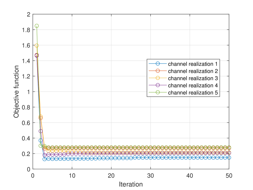
(a) Convergence under different channel realizations

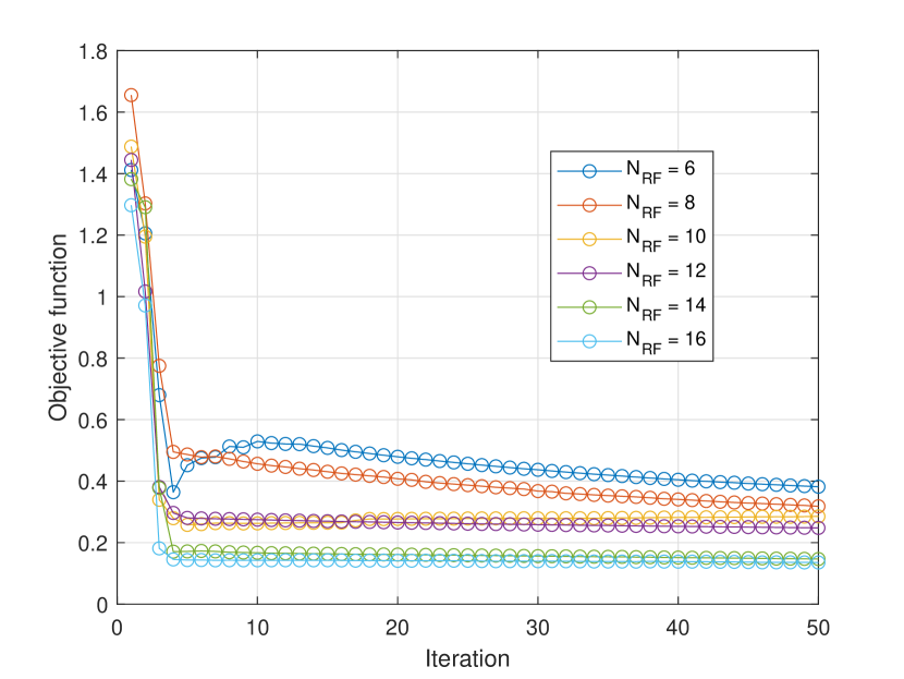
(b) Convergence under varying number of RF chains

Figure 2: Convergence of the manifold-based ADMM algorithm

IV-B Beampattern Performance

In this sub-section, we illustrate the beampattern obtained by the proposed algorithm and compare it with the reference beampattern and the other three benchmark schemes to measure the sensing performance. Fig. 3 shows the designed beampatterns across all the eight sub-carriers. The curve denoted as ‘reference’ represents the reference beampattern, which is identical for all sub-carriers. We observe that the designed beampatterns obtained by our proposed algorithm have main lobes pointing to the directions of interest. The gap of beampattern gain between the reference and designed beampattern exists because the reference beampattern is generated with the total transmit power only for sensing, while in the designed JCAS system, sensing and communication are both realized and only part of the transmit power is used for sensing.

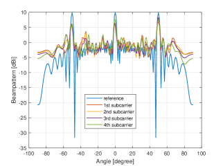
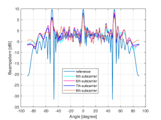
Figure 3: Beampattern for each of the sub-carriers

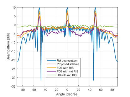
Figure 4: Beampatterns under different schemes

In Fig. 4, the beampatterns obtained from different schemes are compared, where the beampattern results are added up over all the sub-carriers. It can be observed that the fully-digital beamforming scheme (‘FDB with RIS’) has higher main lobes than the corresponding hybrid beamforming scheme (proposed scheme), showing a -10.8 dB beampattern MSE gap. This higher performance is reached at the cost of consuming ${N_{RF}}=N_{t}=64$ RF chains, which is much more than the number of RF chains ${N_{RF}}=16$ used in hybrid beamforming. Besides, the beampatterns obtained by the schemes with random RIS are worse than the corresponding schemes with optimized RIS. Particularly, the beampattern MSE between ‘FDB with RIS’ scheme and ‘FDB with rnd RIS’ scheme is -3.38 dB. The ‘HB with rnd RIS’ scheme does not have an obvious beampattern due to random RIS configuration.

IV-C System Performance under Varying Parameters

In this section, we evaluate the impact of the number of UEs, RIS size, SINR threshold, and SNR on the system performance. In particular, we use the SINR feasibility ratio for communication, and beampattern MSE or PSLR for sensing as a means of comparison.

IV-C1 Impact of number of UEs

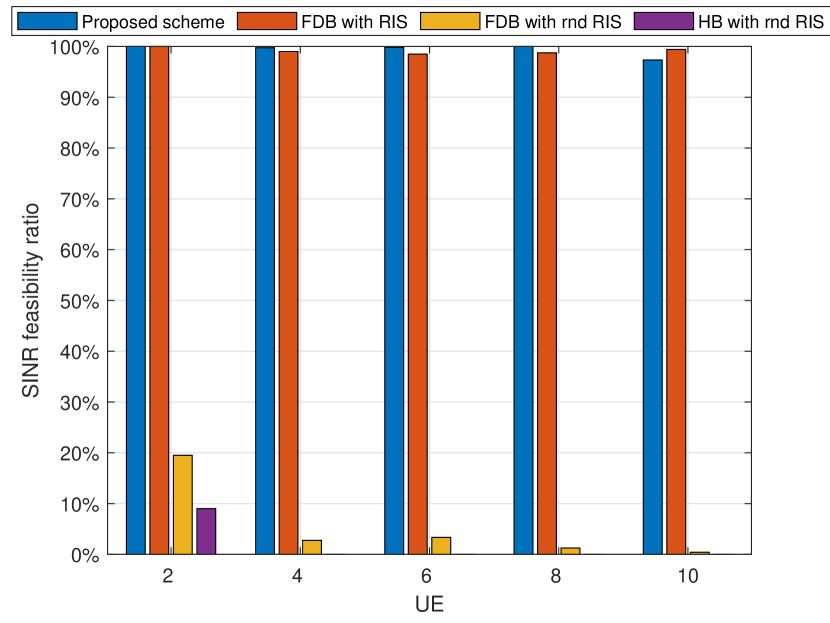
(a) SINR feasibility ratio

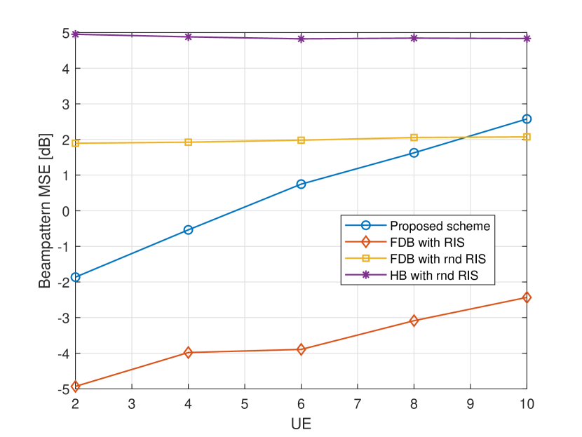
(b) Beampattern MSE at the RIS

Figure 5: SINR feasibility ratio and beampattern MSE at the RIS under a varying number of UEs.

Fig. 5 shows the SINR feasibility ratio and beampattern MSE at the RIS as a function of the number of UEs. In the proposed scheme and ‘FDB with RIS’ scheme, when the number of UEs increases, the SINR feasibility ratio almost maintains 100% while the beampattern MSE worsens. This is because when the number of UEs increases, the multi-user interference on each sub-carrier increases as well. With the provision of the same transmit power, it becomes more difficult to satisfy the SINR constraints for all the UEs on all the sub-carriers. Therefore, more transmit power is allocated to UEs to compensate for the higher multi-user interference and thus to meet the SINR requirements. Consequently, less power remains available for sensing, thus leading to worse beampatterns. Besides, the SINR feasibility ratio and beampattern MSE of the proposed scheme are superior to those of ‘FDB with rnd RIS’ scheme and ‘HB with rnd RIS’ scheme. In particular, the proposed scheme has at least 80.5% SINR feasibility improvement and 26.54% beampattern MSE improvement compared to the two random RIS schemes, demonstrating that the existence of RIS improves the sensing and communication performances. Furthermore, the ‘FDB with RIS’ scheme has a slightly worse SINR feasibility ratio than the proposed scheme. This is because the alternating optimization framework leveraged in the ‘FDB with RIS’ scheme gets stuck in the local optimum.

IV-C2 Impact of number of RIS elements

To achieve better beamforming with more RIS elements, i.e., narrower beamwidth and higher gain, we generate the reference beampattern at the RIS based on the RIS size. In particular, more RIS elements result in a reference beampattern with narrower beamwidth and higher gain. Therefore, under different RIS sizes, the beampattern MSE obtained by different reference beampatterns can not be compared against each other. In this case, the metric average PSLR is employed for sensing performance comparison, measuring the ratio of the main lobe to the side lobe. Fig. 6 illustrates the SINR feasibility ratio and beampattern PSLR versus the number of RIS elements. We observe that the average PSLRs in the proposed scheme and two fully-digital schemes increase as the RIS size increases. Besides, in our proposed scheme, the SINR feasibility ratio improves slightly when there are more RIS phase shifts. In contrast, the SINR feasibility ratio in schemes with random RIS phase shifts reduces by at least 74% compared to the proposed scheme and does not show a regular pattern due to the random RIS phase configuration. Therefore, by including the RIS, the sensing and communication performances can be improved. In addition, more RIS elements result in higher performance improvement.

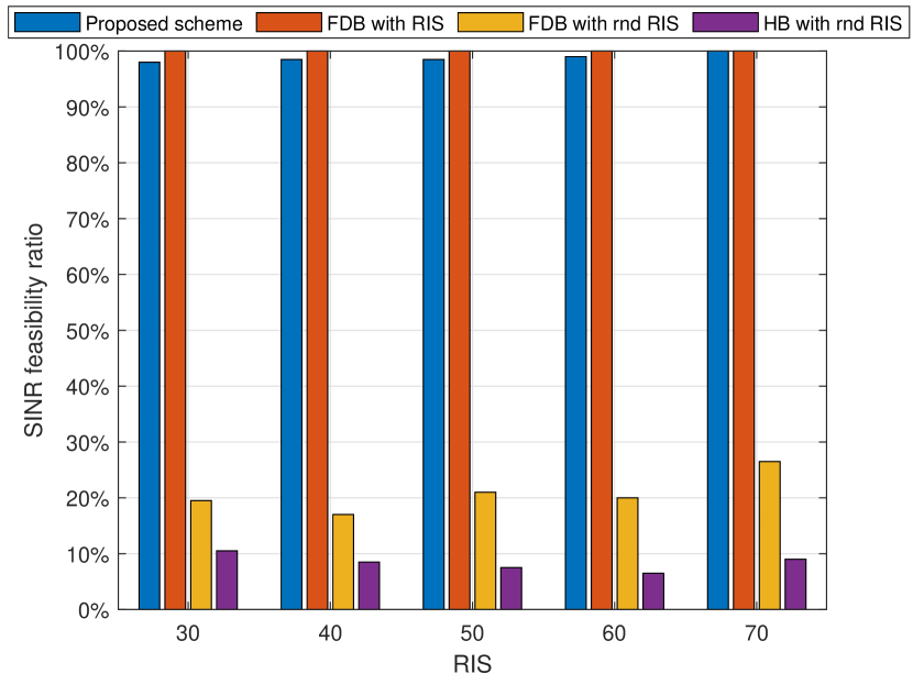
(a) SINR feasibility ratio

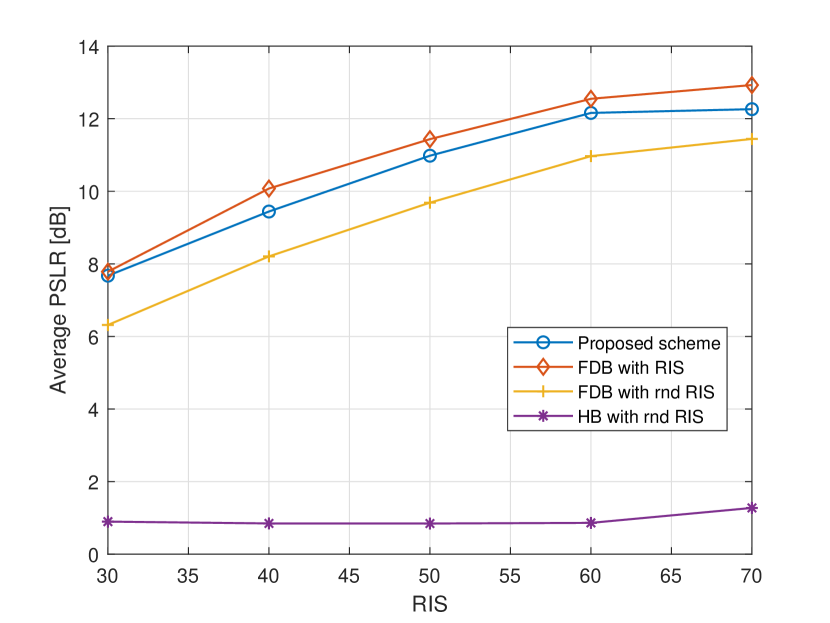
(b) Beampattern PSLR at the RIS at the RIS

Figure 6: SINR feasibility ratio and beampattern PSLR at the RIS under varying RIS sizes

IV-C3 Impact of SINR threshold

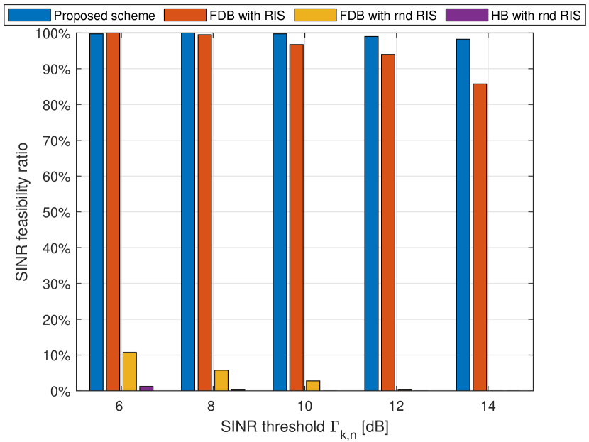
(a) SINR feasibility ratio

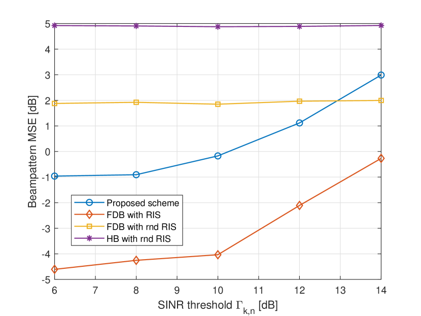
(b) Beampattern MSE at the RIS

Figure 7: SINR feasibility ratio and beampattern MSE at the RIS under varying SINR requirements.

In Fig. 7, the influence of SINR threshold on the sensing and communication performances is shown. We observe that our proposed scheme and ‘FDB with RIS’ scheme can reach a feasible solution when the SINR threshold ${\Gamma_{n,k}}$ is below 12 dB. Beyond this threshold, we can use other measures, e.g., improving the transmit power or utilizing more RIS elements to reach a feasible solution. The SINR feasibility ratio of ‘FDB with RIS’ scheme is lower than the proposed scheme for the same reason as explained in Fig. 5(a), namely being stuck in the local optimum by the alternating optimization used in ‘FDB with RIS’ scheme. In contrast, the SINR performance of schemes with random RIS phase shifts is close to zero, because the RIS configuration does not contribute to improving communication. Besides, the beampattern MSEs of our proposed scheme and ‘FDB with RIS’ scheme increase as the SINR threshold grows. This is due to the fact that a higher transmit power is consumed to support the higher SINR requirements, leaving less transmit power for sensing.

IV-C4 Impact of SNR

Fig. 8 illustrates the impact of SNR on the sensing and communication performance. It can be observed that a higher SNR results in an increasing SINR feasibility ratio under the proposed scheme, ‘FDB with RIS’ scheme and ‘FDB with rnd RIS’ scheme. This is because, for a fixed transmit power, the noise power becomes smaller under a higher SNR, hence the SINR requirements are easier to be satisfied. Besides, the beampattern MSEs of our proposed scheme and ‘FDB with RIS’ scheme gradually decrease as the SNR increases. The reason is that the SINR can be satisfied more easily under a larger SNR, thus leaving more power to optimize sensing.

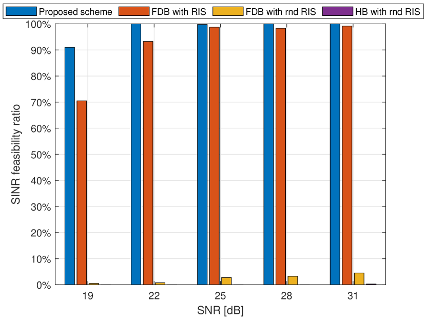
(a) SINR feasibility ratio

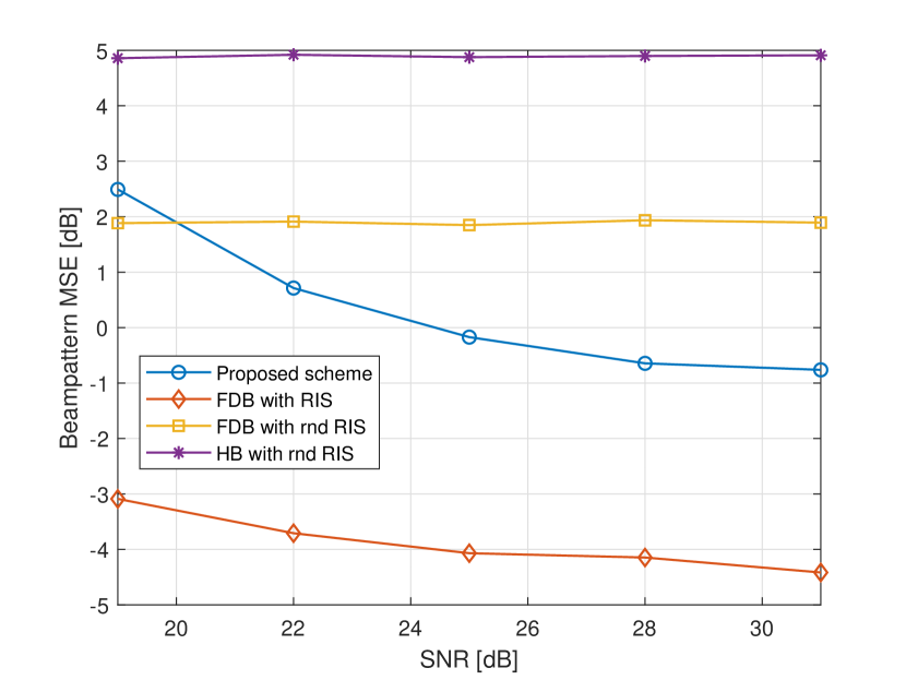
(b) Beampattern MSE at the RIS

Figure 8: SINR feasibility ratio and beampattern MSE at the RIS under varying

In conclusion, in this section, we provide different parameter settings to evaluate their impact on both communication performance and sensing performance. From the simulation results, it can be observed that the sensing goal and communication SINR requirements can be satisfied by configuring suitable system parameters.

IV-D Tradeoff between Communication and Sensing

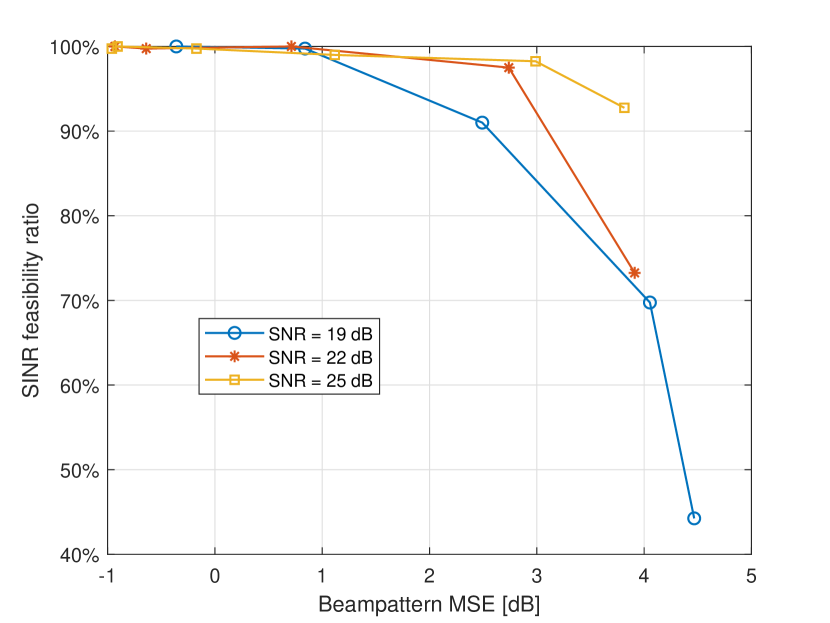
(a) Beampattern MSE at the RIS versus SINR feasibility ratio

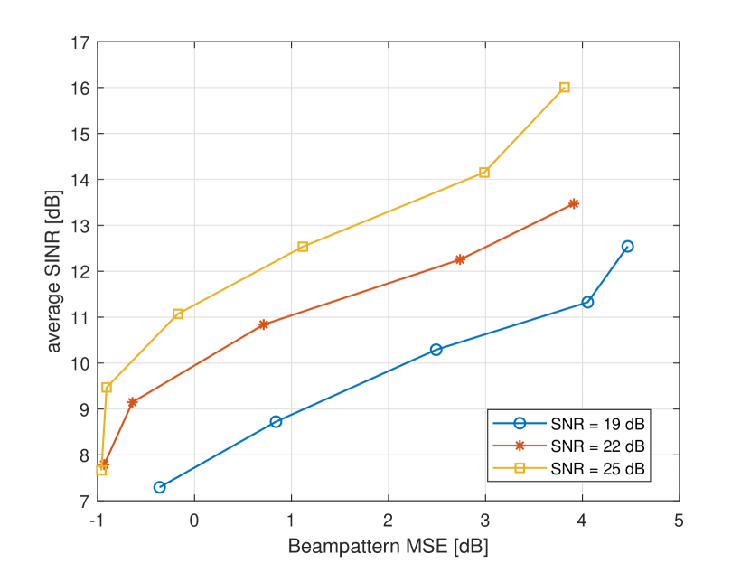
(b) Beampattern MSE at the RIS versus Average SINR

Figure 9: Tradeoff between communication performance and sensing performance

In this section, we measure the tradeoff between sensing performance and communication performance by analyzing the SINR feasibility ratio, the average SINR of all the UEs over all the sub-carriers, and the beampattern MSE, see Fig. 9. It is observed that reaching a higher beampattern MSE corresponds to a lower SINR feasibility ratio and a higher average SINR, i.e., improving communication performance has a negative impact on the sensing performance. For instance, in Fig. 9, we can notice that when SNR = 19 dB, reducing the beampattern MSE by 1.56 dB improves the SINR feasibility ratio by 21% and decreases the average SINR by 1.04 dB. Furthermore, given a higher SNR, a higher average SINR or a lower beampattern MSE can be obtained. For example, in Fig. 9(b), when the SNR increases from 19 dB to 25 dB, up to 1.61 dB average SINR increment and 2.94 dB beampattern MSE increment are achieved. Hence, different tradeoffs between sensing performance and communication performance can be reached under different parameter configurations. For practical usage, the performances of communication and sensing can be weighed according to the required applications.

V Conclusion

In this paper, we investigated the potential of RIS to improve the sensing and communication capabilities of the OFDM JCAS system at mmWave bands. To maximize the performance of sensing and communication, we formulated an optimization model via the joint hybrid beamforming and RIS phase shift design, in order to minimize the difference between the reference beampattern and the designed beampattern at the RIS subject to the power and SINR constraints. By introducing an auxiliary variable and leveraging the penalty method, a manifold-based ADMM algorithm was proposed to solve the formulated non-convex problem. Simulation results demonstrated that our proposed scheme can improve the SINR feasibility ratio for communication and the beampattern PSLR for sensing under larger RIS size. The tradeoff between sensing performance and communication performance was also discussed. As future work, we plan to model the mobility of targets and investigate its impact on the sensing performance.

References

- [1] F. Liu, Y. Cui, C. Masouros, J. Xu, T. X. Han, Y. C. Eldar, and S. Buzzi, “Integrated sensing and communications: Towards dual-functional wireless networks for 6G and beyond,” IEEE J. Sel. Areas Commun., vol. 40, no. 6, pp. 1728–1767, Jun. 2022.
- [2] A. Ali, N. Gonzalez-Prelcic, R. W. Heath, and A. Ghosh, “Leveraging sensing at the infrastructure for mmWave communication,” IEEE Communications Magazine, vol. 58, no. 7, pp. 84–89, Jul, 2020.
- [3] C. Shi, F. Wang, M. Sellathurai, J. Zhou, and S. Salous, “Power minimization-based robust OFDM radar waveform design for radar and communication systems in coexistence,” IEEE Trans. Signal Process., vol. 66, no. 5, pp. 1316–1330, Mar. 2018.
- [4] F. Liu, C. Masouros, A. Li, H. Sun, and L. Hanzo, “MU-MIMO communications with MIMO radar: From co-existence to joint transmission,” IEEE Trans. Wireless Commun., vol. 17, no. 4, pp. 2755–2770, Apr. 2018.
- [5] F. Liu, L. Zhou, C. Masouros, A. Li, W. Luo, and A. Petropulu, “Toward dual-functional radar-communication systems: Optimal waveform design,” IEEE Trans. Signal Process., vol. 66, no. 16, pp. 4264–4279, Jun. 2018.
- [6] L. Chen, F. Liu, W. Wang, and C. Masouros, “Joint radar-communication transmission: A generalized Pareto optimization framework,” IEEE Trans. Signal Process., vol. 69, pp. 2752–2765, May 2021.
- [7] F. Liu, Y.-F. Liu, A. Li, C. Masouros, and Y. C. Eldar, “Cramér-rao bound optimization for joint radar-communication beamforming,” IEEE Trans. Signal Process., vol. 70, pp. 240–253, Dec. 2021.
- [8] X. Liu, T. Huang, N. Shlezinger, Y. Liu, J. Zhou, and Y. C. Eldar, “Joint transmit beamforming for multiuser MIMO communications and MIMO radar,” IEEE Trans. Signal Process., vol. 68, pp. 3929–3944, Jun. 2020.
- [9] H. Hua, J. Xu, and T. X. Han, “Optimal transmit beamforming for integrated sensing and communication,” arXiv preprint arXiv:2104.11871, 2021.
- [10] L. Pucci, E. Paolini, and A. Giorgetti, “System-level analysis of joint sensing and communication based on 5G new radio,” IEEE J. Sel. Areas Commun., Mar. 2022.
- [11] Q. Zhang, Z. Li, X. Gao, and Z. Feng, “Performance evaluation of radar and communication integrated system for autonomous driving vehicles,” in IEEE Conference on Computer Communications Workshops (INFOCOM WKSHPS). IEEE, 2021, pp. 1–2.
- [12] J. Zhang, Y. Huang, J. Wang, X. You, and C. Masouros, “Intelligent interactive beam training for millimeter wave communications,” IEEE Trans. Wireless Commun., vol. 20, no. 3, pp. 2034–2048, Nov. 2020.
- [13] F. Liu and C. Masouros, “Hybrid beamforming with sub-arrayed MIMO radar: Enabling joint sensing and communication at mmWave band,” in IEEE International Conference on Acoustics, Speech and Signal Processing (ICASSP). IEEE, 2019, pp. 7770–7774.
- [14] Z. Cheng, Z. He, and B. Liao, “Hybrid beamforming design for OFDM dual-function radar-communication system,” IEEE J. Sel. Topics Signal Process., vol. 15, no. 6, pp. 1455–1467, Nov. 2021.
- [15] B. Wang, Z. Cheng, and Z. He, “Manifold optimization for hybrid beamforming in dual-function radar-communication system,” Multidimensional Systems and Signal Processing, vol. 34, no. 1, pp. 1–24, 2023.
- [16] Z. Cheng, Z. He, and B. Liao, “Hybrid beamforming for multi-carrier dual-function radar-communication system,” IEEE Trans. Cognitive Commun. and Network., vol. 7, no. 3, pp. 1002–1015, Sept. 2021.
- [17] Z. Cheng and B. Liao, “QoS-aware hybrid beamforming and DOA estimation in multi-carrier dual-function radar-communication systems,” IEEE J. Sel. Areas Commun., vol. 40, no. 6, pp. 1890–1905, Jun. 2022.
- [18] F. Liu, W. Yuan, C. Masouros, and J. Yuan, “Radar-assisted predictive beamforming for vehicular links: Communication served by sensing,” IEEE Trans. Wireless Commun., vol. 19, no. 11, pp. 7704–7719, Nov. 2020.
- [19] Q. Wu, S. Zhang, B. Zheng, C. You, and R. Zhang, “Intelligent reflecting surface-aided wireless communications: A tutorial,” IEEE Trans. Commun., vol. 69, no. 5, pp. 3313–3351, Jan. 2021.
- [20] M. Hua, Q. Wu, D. W. K. Ng, J. Zhao, and L. Yang, “Intelligent reflecting surface-aided joint processing coordinated multipoint transmission,” IEEE Trans. Commun., vol. 69, no. 3, pp. 1650–1665, Mar. 2020.
- [21] Q. Wu and R. Zhang, “Intelligent reflecting surface enhanced wireless network via joint active and passive beamforming,” IEEE Trans. Wireless Commun., vol. 18, no. 11, pp. 5394–5409, Nov. 2019.
- [22] M. Zeng, E. Bedeer, O. A. Dobre, P. Fortier, Q.-V. Pham, and W. Hao, “Energy-efficient resource allocation for IRS-assisted multi-antenna uplink systems,” IEEE Wireless Communications Letters, vol. 10, no. 6, pp. 1261–1265, Jun. 2021.
- [23] W. Ni, X. Liu, Y. Liu, H. Tian, and Y. Chen, “Resource allocation for multi-cell IRS-aided NOMA networks,” IEEE Trans. Wireless Commun., vol. 20, no. 7, pp. 4253–4268, Jul. 2021.
- [24] Z. Chu, P. Xiao, M. Shojafar, D. Mi, J. Mao, and W. Hao, “Intelligent reflecting surface assisted mobile edge computing for Internet of things,” IEEE Wireless Communications Letters, vol. 10, no. 3, pp. 619–623, Nov. 2020.
- [25] Q. Wu and R. Zhang, “Joint active and passive beamforming optimization for intelligent reflecting surface assisted SWIPT under QoS constraints,” IEEE J. Sel. Areas Commun., vol. 38, no. 8, pp. 1735–1748, Aug. 2020.
- [26] S. Buzzi, E. Grossi, M. Lops, and L. Venturino, “Foundations of MIMO radar detection aided by reconfigurable intelligent surfaces,” IEEE Trans. Signal Process., vol. 70, pp. 1749–1763, Mar. 2022.
- [27] Z. Esmaeilbeig, K. V. Mishra, and M. Soltanalian, “IRS-aided radar: Enhanced target parameter estimation via intelligent reflecting surfaces,” in IEEE 12th Sensor Array and Multichannel Signal Processing Workshop (SAM). IEEE, 2022, pp. 286–290.
- [28] J. Hu, H. Zhang, B. Di, L. Li, K. Bian, L. Song, Y. Li, Z. Han, and H. V. Poor, “Reconfigurable intelligent surface based RF sensing: Design, optimization, and implementation,” IEEE J. Sel. Areas Commun., vol. 38, no. 11, pp. 2700–2716, Nov. 2020.
- [29] X. Shao, C. You, W. Ma, X. Chen, and R. Zhang, “Target sensing with intelligent reflecting surface: Architecture and performance,” IEEE J. Sel. Areas Commun., Mar. 2022.
- [30] X. Song, J. Xu, F. Liu, T. X. Han, and Y. C. Eldar, “Intelligent reflecting surface enabled sensing: Cramér-rao bound optimization,” arXiv preprint arXiv:2207.05611, 2022.
- [31] K. Meng, Q. Wu, R. Schober, and W. Chen, “Intelligent reflecting surface enabled multi-target sensing,” IEEE Trans. Commun., vol. 70, no. 12, pp. 8313–8330, 2022.
- [32] H. Zhang, H. Zhang, B. Di, K. Bian, Z. Han, and L. Song, “Metaradar: Multi-target detection for reconfigurable intelligent surface aided radar systems,” IEEE Trans. Wireless Commun., vol. 21, no. 9, pp. 6994–7010, 2022.
- [33] X. Wang, Z. Fei, Z. Zheng, and J. Guo, “Joint waveform design and passive beamforming for RIS-assisted dual-functional radar-communication system,” IEEE Trans. Veh. Tech, vol. 70, no. 5, pp. 5131–5136, May 2021.
- [34] X. Wang, Z. Fei, J. Huang, and H. Yu, “Joint waveform and discrete phase shift design for RIS-assisted integrated sensing and communication system under Cramér-Rao bound constraint,” IEEE Trans. Veh. Tech, vol. 71, no. 1, pp. 1004–1009, Oct. 2021.
- [35] H. Luo, R. Liu, M. Li, Y. Liu, and Q. Liu, “Joint beamforming design for RIS-assisted integrated sensing and communication systems,” IEEE Trans. Veh. Tech, vol. 71, no. 12, pp. 13 393–13 397, 2022.
- [36] M. Hua, Q. Wu, C. He, S. Ma, and W. Chen, “Joint active and passive beamforming design for IRS-aided radar-communication,” IEEE Trans. Wireless Commun., 2022.
- [37] Z. Zhu, Z. Li, Z. Chu, G. Sun, W. Hao, P. Xiao, and I. Lee, “Intelligent reflecting surface assisted integrated sensing and communications for mmwave channels,” arXiv preprint arXiv:2202.00552, 2022.
- [38] R. P. Sankar, B. Deepak, and S. P. Chepuri, “Joint communication and radar sensing with reconfigurable intelligent surfaces,” in IEEE 22nd International Workshop on Signal Processing Advances in Wireless Communications (SPAWC). IEEE, 2021, pp. 471–475.
- [39] Z. Xing, R. Wang, and X. Yuan, “Joint active and passive beamforming design for reconfigurable intelligent surface enabled integrated sensing and communication,” IEEE Trans. Commun., 2023.
- [40] X. Meng, F. Liu, S. Lu, S. P. Chepuri, and C. Masouros, “RIS-assisted integrated sensing and communications: A subspace rotation approach,” arXiv preprint arXiv:2210.13987, 2022.
- [41] T. Wei, L. Wu, K. V. Mishra, and M. Shankar, “Multi-IRS-aided doppler-tolerant wideband DFRC system,” arXiv preprint arXiv:2207.02157, 2022.
- [42] R. Liu, M. Li, Y. Liu, Q. Wu, and Q. Liu, “Joint transmit waveform and passive beamforming design for RIS-aided DFRC systems,” IEEE J. Sel. Topics Signal Process., May 2022.
- [43] Z. Wang, X. Mu, and Y. Liu, “STARS enabled integrated sensing and communications,” IEEE Trans. Wireless Commun., 2023.
- [44] R. Liu, M. Li, Q. Liu, and A. L. Swindlehurst, “SNR/CRB-constrained joint beamforming and reflection designs for RIS-ISAC systems,” arXiv preprint arXiv:2301.11134, 2023.
- [45] X. Song, T. X. Han, and J. Xu, “Cramér-Rao bound minimization for IRS-enabled multiuser integrated sensing and communication with extended target,” arXiv preprint arXiv:2210.16592, 2022.
- [46] M. Hua, Q. Wu, W. Chen, O. A. Dobre, and A. L. Swindlehurst, “Secure intelligent reflecting surface aided integrated sensing and communication,” arXiv preprint arXiv:2207.09095, 2022.
- [47] X. Song, D. Zhao, H. Hua, T. X. Han, X. Yang, and J. Xu, “Joint transmit and reflective beamforming for IRS-assisted integrated sensing and communication,” in IEEE Wireless Communications and Networking Conference (WCNC). IEEE, 2022, pp. 189–194.
- [48] R. P. Sankar and S. P. Chepuri, “Beamforming in hybrid RIS assisted integrated sensing and communication systems,” in 30th European Signal Processing Conference (EUSIPCO). IEEE, 2022, pp. 1082–1086.
- [49] R. Sankar, S. P. Chepuri, and Y. C. Eldar, “Beamforming in integrated sensing and communication systems with reconfigurable intelligent surfaces,” arXiv preprint arXiv:2206.07679, 2022.
- [50] G. Zhang, C. Shen, F. Liu, Y. Lin, and Z. Zhong, “Beampattern design for RIS-aided dual-functional radar and communication systems,” in IEEE Global Communications Conference. IEEE, 2022, pp. 3899–3904.
- [51] H. Zhang, “Joint waveform and phase shift design for RIS-assisted integrated sensing and communication based on mutual information,” IEEE Communications Letters, vol. 26, no. 10, pp. 2317–2321, 2022.
- [52] X. Liu, H. Zhang, K. Long, M. Zhou, Y. Li, and H. V. Poor, “Proximal policy optimization-based transmit beamforming and phase-shift design in an IRS-aided ISAC System for the THz band,” IEEE J. Sel. Areas Commun., Mar. 2022.
- [53] F. Sohrabi and W. Yu, “Hybrid analog and digital beamforming for mmWave OFDM large-scale antenna arrays,” IEEE J. Sel. Areas Commun., vol. 35, no. 7, pp. 1432–1443, Jul. 2017.
- [54] Q. Wu and R. Zhang, “Beamforming optimization for wireless network aided by intelligent reflecting surface with discrete phase shifts,” IEEE Trans. Commun., vol. 68, no. 3, pp. 1838–1851, Dec. 2019.
- [55] Y.-P. Lin, “Hybrid MIMO-OFDM beamforming for wideband mmwave channels without instantaneous feedback,” IEEE Trans. Signal Process., vol. 66, no. 19, pp. 5142–5151, Aug. 2018.
- [56] Z. Wang, L. Liu, and S. Cui, “Channel estimation for intelligent reflecting surface assisted multiuser communications: Framework, algorithms, and analysis,” IEEE Trans. Wireless Commun., vol. 19, no. 10, pp. 6607–6620, Jun. 2020.
- [57] P.-A. Absil and K. A. Gallivan, “Joint diagonalization on the oblique manifold for independent component analysis,” in IEEE international conference on acoustics speech and signal processing proceedings (ICASSP), vol. 5. IEEE, 2006, pp. 945–948.
- [58] N. Boumal, “An introduction to optimization on smooth manifolds,” Available online, May, vol. 3, 2020.