Quantitative Metrics for Evaluating Explanations of Video DeepFake Detectors

Abstract

The proliferation of DeepFake technology is a rising challenge in today’s society, owing to more powerful and accessible generation methods. To counter this, the research community has developed detectors of ever-increasing accuracy. However, the ability to explain the decisions of such models to users is lacking behind and is considered an accessory in large-scale benchmarks, despite being a crucial requirement for the correct deployment of automated tools for content moderation. We attribute the issue to the reliance on qualitative comparisons and the lack of established metrics. We describe a simple set of metrics to evaluate the visual quality and informativeness of explanations of video DeepFake classifiers from a human-centric perspective. With these metrics, we compare common approaches to improve explanation quality and discuss their effect on both classification and explanation performance on the recent DFDC and DFD datasets.

1 Introduction

“DeepFake” refers to the realistic alteration or generation of multimedia content, in visual, audio, or textual form. The most striking application of DeepFakes are generative deep learning models that can alter a person’s appearance in videos. From early attempts [Thies et al.(2016)Thies, Zollhofer, Stamminger, Theobalt, and Niessner, Suwajanakorn et al.(2017)Suwajanakorn, Seitz, and Kemelmacher-Shlizerman], the quality of these face-swapping techniques has increased consistently to the point that both casual and attentive observers can be fooled. While some applications can be positively innovating [Westerlund(2019)], DeepFakes can be designed with malicious intent, such as online disinformation or public defamation. In response, the research community has introduced datasets [Rossler et al.(2019)Rossler, Cozzolino, Verdoliva, Riess, Thies, and Niessner, Nick Dufour and Andrew Gully(2019), Dolhansky et al.(2020)Dolhansky, Bitton, Pflaum, Lu, Howes, Wang, and Ferrer, Pu et al.(2021)Pu, Mangaokar, Kelly, Bhattacharya, Sundaram, Javed, Wang, and Viswanath] and methods [Coccomini et al.(2021)Coccomini, Messina, Gennaro, and Falchi, Bonettini et al.(2021)Bonettini, Cannas, Mandelli, Bondi, Bestagini, and Tubaro, Kim et al.(2021)Kim, Tariq, and Woo] for the automatic monitoring and detection of DeepFakes. However, benchmark performance has become the de-facto goal, shadowing other aspects that are crucial for the correct deployment of such models.

In practice, as automated DeepFake detectors acquire a significant role for moderation and censorship of online communities, it becomes necessary to inspect and explain their decision process. From the users’ perspective, it is not acceptable that “black-box” models manage their freedom of expression and online safety. Instead, users require intuitive explanations to validate DeepFake forgeries, prevent unjustified censorship, and trust automated moderation systems. From the perspective of companies and regulators, interpretability is necessary to justify the enforcement of DeepFake detectors, in accordance to the right to explanation of legal frameworks such as the GDPR [European Union(2018)]. Also, developers of such tools can benefit from explanations to verify the learned representation, mitigate unwanted bias, and defend against adversarial attacks.

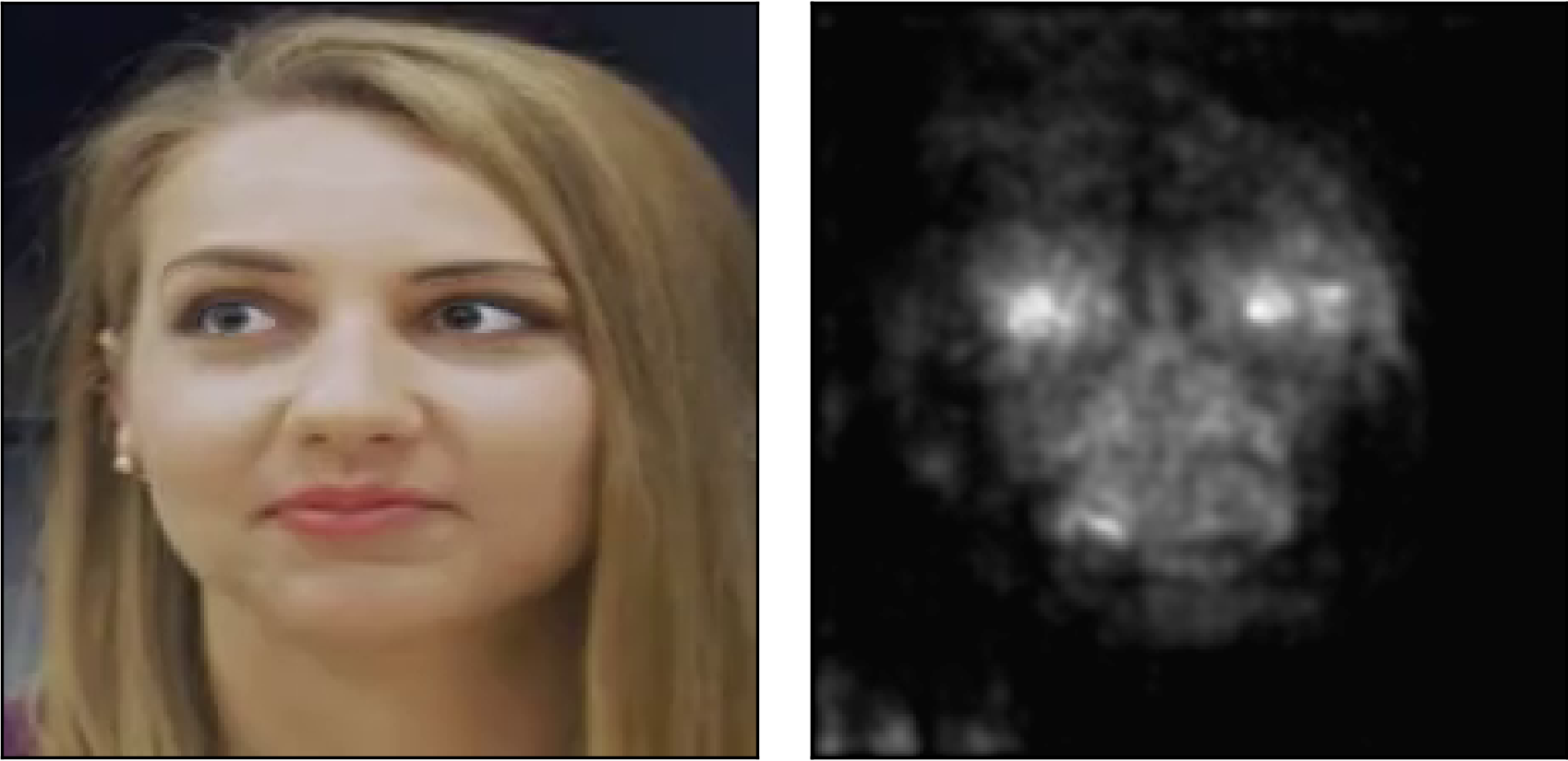
Figure 1: Explanation heatmap for one sample from DeepFake Dataset obtained by applying SmoothGrad to a classifier regularized with Total Variation. The resulting heatmap is visually smooth ($\text{TV}=0.25$), localized ($\sigma=731$), and concentrates around visible manipulation artefacts ($M_{\text{in}}=18.1\%$), i.ethe eyes and one corner of the mouth.

Several methods for explaining visual classifiers exist, e.g [Simonyan et al.(2014)Simonyan, Vedaldi, and Zisserman, Selvaraju et al.(2020)Selvaraju, Cogswell, Das, Vedantam, Parikh, and Batra], which can be compared in terms of faithfulness to the model and correctness to the data. However, researchers lack quantitative tools to evaluate human-centric properties of explanations and claims of improved informativeness are often based on subjective comparisons. This work introduces a quantitative framework to evaluate DeepFake explanations w.r.tto human perception, which can be applied in practical deployments of DeepFake classifiers. In particular, we contextualize existing metrics, i.emanipulation detection, and propose new ones as needed, namely for smoothness, sparsity, and locality. We apply these metrics to state-of-the-art video recognition models and compare several techniques intended for improving explanations, forming a quantitative baseline on the DeepFake Detection Challenge dataset and the DeepFake Dataset [Rossler et al.(2019)Rossler, Cozzolino, Verdoliva, Riess, Thies, and Niessner, Dolhansky et al.(2020)Dolhansky, Bitton, Pflaum, Lu, Howes, Wang, and Ferrer]. Last, we empirically evaluate how to best communicate heatmap-based explanations to users, discuss limitations and future directions for DeepFake explainability.

2 Related work

DeepFake generation.

Since their inception, generative models have been applied to manipulate faces, bodies and voices in online media. Today’s availability of online content and ease of access to open-source frameworks, allow anyone with consumer-grade hardware to generate DeepFakes. While legitimate applications of this technology exits, e.gdubbing, DeepFakes have been infamously used for disinformation, fraud, hatred, sexual abuse, and other crimes [Damiani(2019), Vaccari and Chadwick(2020)]. This work focuses on visual forgery of faces in videos, which can be categorized as face swapping, in which the appearance of a face is replaced with another [Nirkin et al.(2018)Nirkin, Masi, Tran, Hassner, and Medioni, Deepfakes Team(2021), Kowalski(2021), Li et al.(2020a)Li, Bao, Yang, Chen, and Wen]; or facial reenactment, in which expressions are edited [Thies et al.(2016)Thies, Zollhofer, Stamminger, Theobalt, and Niessner, Thies et al.(2019)Thies, Zollhöfer, and Nießner]. Such manipulations can be produced via purely learning-based generative models [Nirkin et al.(2019)Nirkin, Keller, and Hassner, Deepfakes Team(2021), Thies et al.(2019)Thies, Zollhöfer, and Nießner] or hybrid computer graphics approaches [Thies et al.(2016)Thies, Zollhofer, Stamminger, Theobalt, and Niessner, Kowalski(2021)]. For survey of methods and applications, we refer the reader to the works of Tolosana et al[Tolosana et al.(2020)Tolosana, Vera-Rodriguez, Fierrez, Morales, and Ortega-Garcia] and Masood et al [Masood et al.(2021)Masood, Nawaz, Malik, Javed, and Irtaza].

DeepFake detection.

In response to the widespread misuse of DeepFakes, researchers and companies have started focusing on automated detection of forged media. Forensic approaches vary from detecting anatomical inconsistencies [Agarwal et al.(2019)Agarwal, Farid, Gu, He, Nagano, and Li, Li et al.(2018)Li, Chang, and Lyu, Li and Lyu(2018)], to analyzing digital artefacts [Afchar et al.(2018)Afchar, Nozick, Yamagishi, and Echizen, Yang et al.(2019)Yang, Li, and Lyu, Matern et al.(2019)Matern, Riess, and Stamminger]. Other approaches are purely learning-based [Güera and Delp(2018), Amerini et al.(2019)Amerini, Galteri, Caldelli, and Del Bimbo] and can integrate advanced architectures and optimization techniques [Nguyen et al.(2019b)Nguyen, Yamagishi, and Echizen, Nguyen et al.(2019a)Nguyen, Fang, Yamagishi, and Echizen, Bondi et al.(2020)Bondi, Daniele Cannas, Bestagini, and Tubaro, Kim et al.(2021)Kim, Tariq, and Woo, Coccomini et al.(2021)Coccomini, Messina, Gennaro, and Falchi]. Key to this effort is the release of large-scale datasets of images [Karras et al.(2019)Karras, Laine, and Aila, Dang et al.(2020)Dang, Liu, Stehouwer, Liu, and Jain, Neves et al.(2020)Neves, Tolosana, Vera-Rodriguez, Lopes, Proença, and Fierrez, Generated Photos Team(2018)], audio [Zhou et al.(2019)Zhou, Liu, Liu, Luo, and Wang], and videos [Rossler et al.(2019)Rossler, Cozzolino, Verdoliva, Riess, Thies, and Niessner, Nick Dufour and Andrew Gully(2019), Li et al.(2020b)Li, Yang, Sun, Qi, and Lyu, Dolhansky et al.(2020)Dolhansky, Bitton, Pflaum, Lu, Howes, Wang, and Ferrer, Pu et al.(2021)Pu, Mangaokar, Kelly, Bhattacharya, Sundaram, Javed, Wang, and Viswanath, Zi et al.(2021)Zi, Chang, Chen, Ma, and Jiang], which allow to train deep models for forgery detection.

Explainable AI.

Although powerful, deep learning models are often deemed “black-boxes” to illustrate the opacity of their decision process. The field of study of Explainable AI (XAI) tries to address these shortcomings to allow users, researchers, and regulators to gain insights into such models (model interpretability) and their outputs (decision explainability) [Gilpin et al.(2018)Gilpin, Bau, Yuan, Bajwa, Specter, and Kagal, Miller(2019)]. In the visual domain, in particular for classification, it is common to explain the decision of a model using heatmaps which highlight important areas of the input [Zeiler and Fergus(2014), Fong and Vedaldi(2017), Petsiuk et al.(2018)Petsiuk, Das, and Saenko]. Backpropagation-based approaches generate heatmaps by computing gradients [Simonyan et al.(2014)Simonyan, Vedaldi, and Zisserman, Zhou et al.(2015)Zhou, Khosla, Lapedriza, Oliva, and Torralba, Smilkov et al.(2017)Smilkov, Thorat, Kim, Viégas, and Wattenberg, Sundararajan et al.(2017)Sundararajan, Taly, and Yan, Kapishnikov et al.(2019)Kapishnikov, Bolukbasi, Viégas, and Terry, Selvaraju et al.(2020)Selvaraju, Cogswell, Das, Vedantam, Parikh, and Batra, Xu et al.(2020)Xu, Venugopalan, and Sundararajan] or gradient surrogates [Springenberg et al.(2015)Springenberg, Dosovitskiy, Brox, and Riedmiller, Montavon et al.(2018)Montavon, Samek, and Müller, Samek et al.(2021)Samek, Montavon, Lapuschkin, Anders, and Müller]. Alternative approaches construct proxy models that are locally faithful and easier to interpret, e.gLIME [Ribeiro et al.(2016)Ribeiro, Singh, and Guestrin]. Recently, transformer models [Vaswani et al.(2017)Vaswani, Shazeer, Parmar, Uszkoreit, Jones, Gomez, Kaiser, and Polosukhin, Dosovitskiy et al.(2020)Dosovitskiy, Beyer, Kolesnikov, Weissenborn, Zhai, Unterthiner, Dehghani, Minderer, Heigold, Gelly, Uszkoreit, and Houlsby, Arnab et al.(2021)Arnab, Dehghani, Heigold, Sun, Lučić, and Schmid] have popularized using attention maps as explanations [Abnar and Zuidema(2020), Chefer et al.(2021)Chefer, Gur, and Wolf, Xu et al.(2015)Xu, Ba, Kiros, Cho, Courville, Salakhudinov, Zemel, and Bengio], although these might not be representative [Jain and Wallace(2019)].

DeepFake explainability.

As social platforms integrate automated tools for DeepFake detection and moderation in their pipelines [Masood et al.(2021)Masood, Nawaz, Malik, Javed, and Irtaza], it becomes crucial to offer proper justification when some content is blocked. Prototype-based explanations as in Trinh et al [Trinh et al.(2021)Trinh, Tsang, Rambhatla, and Liu], could teach users to identify manipulation artefacts on their own. Similarly, SHAP-based methods can be adapted to to videos by defining 3D super-pixels [Lundberg and Lee(2017), Pino et al.(2021)Pino, Carman, and Bestagini]. Focusing on input features, Wang et al [Wang et al.(2021)Wang, Oramas, and Tuytelaars] suggest pre-processing steps that result in more human-interpretable heatmaps, according to a qualitative evaluation. Finally, human-annotated explanations, e.gMathew et al [Mathew et al.(2020)Mathew, Saha, Yimam, Biemann, Goyal, and Mukherjee], provide direct insight on manipulation techniques.

3 Method

3.1 Explanations methods

Our goal is to establish quantitative metrics to evaluate explanations of visual DeepFake classifiers. In particular, we focus on heatmap-based methods [Simonyan et al.(2014)Simonyan, Vedaldi, and Zisserman, Zeiler and Fergus(2014), Bach et al.(2015)Bach, Binder, Montavon, Klauschen, Müller, and Samek] that associate each pixel to a scalar proportionally to its importance w.r.tthe classifier decision. Formally, we define a video $v\in\mathcal{V}$ as a mapping from a discrete grid $\mathcal{G}=T\!\times\!H\!\times\!W$ to the RGB color space. A DeepFake classifier is then a function $f:\mathcal{V}\rightarrow[0,1]$ that maps a video to the probability distribution $p(\textsc{fake}|v)$. An explanation method is a function $\Phi:\mathcal{V}\times\mathcal{F}\to\mathcal{H}$ that maps a pair $(v,f)$ to a relevance heatmap $h:\mathcal{G}\rightarrow\mathbb{R}^{+}$, where $\mathcal{F}$ and $\mathcal{H}=\{h|\int hd\lambda=1\}$ denote the set of classifiers and heatmaps respectively. With this notation, popular gradient-based explanation methods are expressed as: Sensitivity $\nabla f(v)$ [Simonyan et al.(2014)Simonyan, Vedaldi, and Zisserman]; Gradient$\times$Input $\nabla f(v)\cdot v$ [Kindermans et al.(2016)Kindermans, Schütt, Müller, and Dähne]; SmoothGrad $\mathbb{E}_{\epsilon\sim\mathcal{N}(0,\delta I)}\left[\nabla f(v+v_{\epsilon})\right]$, where $v_{\epsilon}$ adds random color perturbations [Smilkov et al.(2017)Smilkov, Thorat, Kim, Viégas, and Wattenberg]; and Integrated Gradients $(v-v_{b})\cdot\int_{0}^{1}\nabla f(v_{b}+\alpha(v-v_{b}))d\alpha$, where the baseline $v_{b}$ is a uniform black video [Sundararajan et al.(2017)Sundararajan, Taly, and Yan]. Note that $\nabla$ and $\int$ are discretized operators over $\mathcal{G}$ (see Appendix D).

Explanation methods are commonly compared according to their faithfulness, i.ethe ability to correctly explain a decision [Bach et al.(2015)Bach, Binder, Montavon, Klauschen, Müller, and Samek, Ribeiro et al.(2016)Ribeiro, Singh, and Guestrin, Montavon et al.(2017)Montavon, Lapuschkin, Binder, Samek, and Müller, Alvarez Melis and Jaakkola(2018), Selvaraju et al.(2020)Selvaraju, Cogswell, Das, Vedantam, Parikh, and Batra]. Faithfulness is quantified by the deletion score [Samek et al.(2017)Samek, Binder, Montavon, Lapuschkin, and Müller, Petsiuk et al.(2018)Petsiuk, Das, and Saenko] defined as $\mathbb{E}_{v}\left[\int f(v\odot(1-h_{\alpha}))d\alpha\right]$, where $h_{\alpha}$ is a binary mask obtained by selecting the most important pixels from the explanation $\Phi(f,v)$ such that their cumulative relevance is $\alpha\in[0,1]$. A low deletion score indicates a faithful explanation method: if relevant pixels are masked out first, the prediction confidence should drop sharply. For our baseline model, SmoothGrad achieves the lowest deletion score (paired one-sided t-test $p<10^{-5}$) and is therefore selected for all evaluations of visual quality. We report per-method hyperparameters and per-dataset scores in Section D.4. Clearly, faithfulness is a necessary property of explanation methods, however, their heatmaps can still appear noisy and uninformative for humans, hence the need for quantitative metrics of visual quality.

3.2 Evaluation metrics

As discussed in Section 2, several works address the representativeness or visual appearance of heatmaps. However, the improvement is often demonstrated through qualitative examples, while quantitative comparison is lacking. Understandably, defining general-purpose metrics for quantifying explanation properties is not trivial [Ancona et al.(2018)Ancona, Ceolini, Öztireli, and Gross], as the perceived quality depends on the data itself, on the target user, and the downstream task. Focussing on explanations of video DeepFake classifiers, we discuss a set of desirable human-centric properties [Koffka(2013), Barredo Arrieta et al.(2020)Barredo Arrieta, Díaz-Rodríguez, Del Ser, Bennetot, Tabik, Barbado, Garcia, Gil-Lopez, Molina, Benjamins, Chatila, and Herrera, Mohseni et al.(2021)Mohseni, Zarei, and Ragan] and formulate quantitative metrics for their evaluation.

3.2.1 Visual quality

The first set of metrics considers general properties of explanation heatmaps that facilitate their understanding and communicability. Complex models can take decisions based on features that are not easily accessible to users, e.gtexture details or high-frequency patterns [Geirhos et al.(2018)Geirhos, Rubisch, Michaelis, Bethge, Wichmann, and Brendel, Wang et al.(2021)Wang, Oramas, and Tuytelaars]. Instead, we expect models that focus on human-interpretable cues [Koffka(2013)] such as small manipulation artefacts, teeth misalignment, non-circular pupils, or irregular skin complexion, to produce smoother, sparser and more localized heatmaps.

Smoothness.

Explanations that vary excessively between neighboring pixels or frames are not meaningful to humans [Wang et al.(2021)Wang, Oramas, and Tuytelaars]. The smoothness of a heatmap $h:\mathcal{G}\to\mathbb{R}^{+}$ is measured as its Total Variation (TV), where low values indicate higher local consistency:

$$\text{TV}(h)=\int_{\mathcal{G}}\lVert\nabla h\rVert_{1}d\lambda.$$ (1)

Spatial locality.

Unambiguous explanations should concentrate on few spatially-close patches of a video, i.etheir relevance should be localized. If we consider $h$ as the distribution of a random vector $\bm{\rho}\in\mathcal{G}$, we can measure locality through the volume of its variance matrix:

$$\sigma=|\det(\bm{\Sigma})|=\left|\det\left(\mathbb{E}_{h}\left[\bm{\rho}\bm{\rho}^{T}\right]-\mathbb{E}_{h}\left[\bm{\rho}\right]\mathbb{E}_{h}\left[\bm{\rho}^{T}\right]\right)\right|.$$ (2)

A low $\sigma$ will favor sharp unimodal distributions, e.ga Gaussian with low dispersion, as opposed to scattered multimodal heatmaps. In the context of DeepFakes, this means highlighting single manipulation artefacts instead of allocating mass to distinct parts of the face. For other tasks, spatial locality can be extended to account for domain-specific requirements.

Sparsity.

While TV and $\sigma$ capture spatial properties, the individual values shall also be sparse, since few highly important regions are more indicative of a good explanation than several mildly relevant ones. Both $L_{0}$ norm and Entropy [Shannon(1948)] are popular measures of sparsity, but the Gini Index [Gini(1912)] is preferred according to Hurley and Rickard [Hurley and Rickard(2009)]. For a heatmap $h:\mathcal{G}\to\mathbb{R}^{+}$ and sorting indices $i=\{1,\ldots,THW\}$ such that $h(\bm{\rho}_{i})\leq h(\bm{\rho}_{i+1})$:

$$\operatorname{G}=\frac{2}{THW}\frac{\sum_{i}i\cdot h(\bm{\rho}_{i})}{\sum_{i}h(\bm{\rho}_{i})}-\frac{THW+1}{THW}.$$ (3)

3.2.2 Manipulation detection

Smooth, sparse and localized heatmaps appear visually appealing, but do they convey the location of manipulation cues? Offering specific evidence greatly increases trust in the model, helps diagnosing failure cases, and encourages users to develop a critical eye for spotting DeepFakes. In the XAI literature, manipulation detection is commonly evaluated through user studies [Selvaraju et al.(2020)Selvaraju, Cogswell, Das, Vedantam, Parikh, and Batra, Wang et al.(2021)Wang, Oramas, and Tuytelaars], which suffers from reproducibility issues, or under a weakly-supervised paradigm [Cao et al.(2015)Cao, Liu, Yang, Yu, Wang, Wang, Huang, Wang, Huang, Xu, Ramanan, and Huang, Kolesnikov and Lampert(2016), Baldassarre et al.(2020)Baldassarre, Smith, Sullivan, and Azizpour, Selvaraju et al.(2020)Selvaraju, Cogswell, Das, Vedantam, Parikh, and Batra], which risk introducing bias from the additional annotations.

We argue that DeepFakes offer a unique possibility for the objective evaluation of weakly-supervised manipulation detection. Given a real video $v_{R}$, its fake(s) $v_{F}$, and a face parsing model $s:\mathcal{G}\rightarrow\mathcal{P}$ that maps pixels of $v_{R}$ to $\mathcal{P}=\{\text{eyes},\text{nose},\text{mouth}\}$, an ad-hoc evaluation sample can be produced such that the manipulation is limited to a specific semantic region:

$$v_{p}(\bm{\rho})=\begin{cases}v_{F}(\bm{\rho})&\mbox{if }s(\bm{\rho})=p\\ v_{R}(\bm{\rho})&\mbox{otherwise}\end{cases}\quad\forall p\in\mathcal{P}$$ (4)

Assuming a well-trained detector and a faithful explanation method, heatmaps for $v_{p}$ should closely match the manipulated region. Since an objective ground-truth is available by construction, it’s possible to assess manipulation detection using common segmentation metrics. First, $M_{\text{in}}$ measures the percentage of heatmap mass inside the ground-truth mask, i.e$\int_{\mathcal{G}}m_{p}(\bm{\rho})h(\bm{\rho})d\lambda$, to ensure that little or no relevance is assigned to non-manipulated regions. Second, precision at 100 ($P_{100}$), i.ethe fraction of the 100 most relevant pixels that falls inside the ground-truth, accounts for manipulation artefacts significantly smaller than the selected region. Additional manipulation detection metrics are reported in Sec. D.5.

As a point of discussion, both humans and computers may “look at” other parts of a video to assess whether one portion is manipulated, e.gnoting the mismatch between a smiling mouth and two frowning eyes. However, when asking “why is the video fake?”, we expect to be pointed at the visible manipulation and not at other natural-looking features. Therefore, in this context, manipulation masks are considered as the ground-truth explanation.

4 Experiments

The previous section establishes a set of desirable qualities of explanations and proposes evaluation metrics built on sound mathematical foundations. We now consider several techniques from previous works and quantify their effect on explanations using these metrics. Section 4.1 analyses the effects of i) data preparation [Wang et al.(2021)Wang, Oramas, and Tuytelaars] ii) loss-based regularization [Rudin et al.(1992)Rudin, Osher, and Fatemi] iii) augmentation-based regularization [DeVries and Taylor(2017)] iv) model architecture [Geirhos et al.(2018)Geirhos, Rubisch, Michaelis, Bethge, Wichmann, and Brendel, Tuli et al.(2021)Tuli, Dasgupta, Grant, and Griffiths] Both and classification performance (Tab. 1) and explanation quality (Fig. 2) are reported for each experiment. Furthermore, Section 4.2 discusses post-processing techniques for heatmap visualization, which are important for communicating explanations to users in practice.

Training dataset.

All models are trained on videos from the DeepFake Detection Challenge [Dolhansky et al.(2020)Dolhansky, Bitton, Pflaum, Lu, Howes, Wang, and Ferrer] in “high-quality” compression (constant rate quantization 23). Specifically, we train on $19k$ real and $100k$ fake videos, and use the official validation split of $2k$ real and $2k$ fakes for hyper-parameter tuning. Each video is preprocessed using the MTCNN face detector [Zhang et al.(2016)Zhang, Zhang, Li, and Qiao], the main face is heuristically determined among all detections, then cropped and resized to $224\!\times\!224$ pixels. Part segmentation is obtained with the BiSeNet face parser [Yu et al.(2021)Yu, Gao, Wang, Yu, Shen, and Sang] and aggregated into background, face, nose, mouth, eyes, ears. Additional details on data preparation and dataset statistics are provided in Appendix A.

Explanation datasets.

For a cross-dataset evaluation of explanation quality metrics we employ a held-out subset of DFDC, which has a distribution similar to training videos, and a subset of the DeepFake Detection Dataset (DFD)[Nick Dufour and Andrew Gully(2019)], which is more challenging due to the potential distribution shift. Visual quality metrics (Sec. 3.2.1) are computed on the explanations of fake videos, while manipulation detection (Sec. 3.2.2) is evaluated on three part-swaps per video, namely eyes, mouth and nose. Notably, manipulation detection can only be evaluated on a subset of temporally and spatially aligned videos due to the part-swapping procedure. Additional details are provided in Appendix A. While the proposed metrics can be flexibly applied to any dataset of real-fake video pairs, we release the code for preprocessing, training and evaluation on DFDC and DFD to encourage comparison and facilitate reproducibility: github.com/baldassarreFe/deepfake-detection.

Classifier.

Our baseline model is a 3D CNN trained with no pre-processing, no regularization and no data augmentation except random color augmentations. Specifically, the backbone feature extractor is an S3D model [Xie et al.(2018)Xie, Sun, Huang, Tu, and Murphy] pre-trained on Kinetics 400 [Kay et al.(2017)Kay, Carreira, Simonyan, Zhang, Hillier, Vijayanarasimhan, Viola, Green, Back, Natsev, Suleyman, and Zisserman]. The output of each convolutional block is pooled, concatenated, and fed to a 2-layer MLP classification head. Such shortcut connections proved beneficial over a sequential model in early experiments, likely due to the multi-scale nature of manipulation artefacts. During training, the AdamW optimizer [Loshchilov and Hutter(2019)] minimizes a cross-entropy loss $\mathcal{L}_{\text{CE}}$ based on binary video labels until a validation loss stops improving. Additional details about hyperparameters and training can be found in Appendix C. For each model variant described below, Table 1 reports the average cross-entropy loss and AUROC over 3 runs on the official test split. While all models achieve satisfactory results on both datasets, performance drops when generalizing from DFDC to DFD. For this reason, we consider explanation metrics evaluated on DFDC more indicative of explanation quality in the following experiments.

Table 1: Classification metrics: $L_{\text{CE}}$ is categorical cross-entropy ($\downarrow$), $A_{\text{ROC}}$ is the area under the receiver operating characteristic curve ($\uparrow$). Average values over 3 runs, full results in Tables 4 and 3. Reported values account for class imbalance as detailed in Table 2.

	DFDC test		DFD
	$\mathcal{L}_{\text{CE}}$	$A_{\text{ROC}}$	$\mathcal{L}_{\text{CE}}$	$A_{\text{ROC}}$
S3D Baseline	.447	89.0	.694	80.2
S3D Bilateral	.696	54.2	.746	45.8
S3D Gaussian	.542	81.8	.760	66.4
S3D TV Loss	.460	87.4	.698	75.8
S3D Cutout	.481	87.2	.655	79.6
MViT	.430	96.4	.513	90.0

4.1 Quantitative results

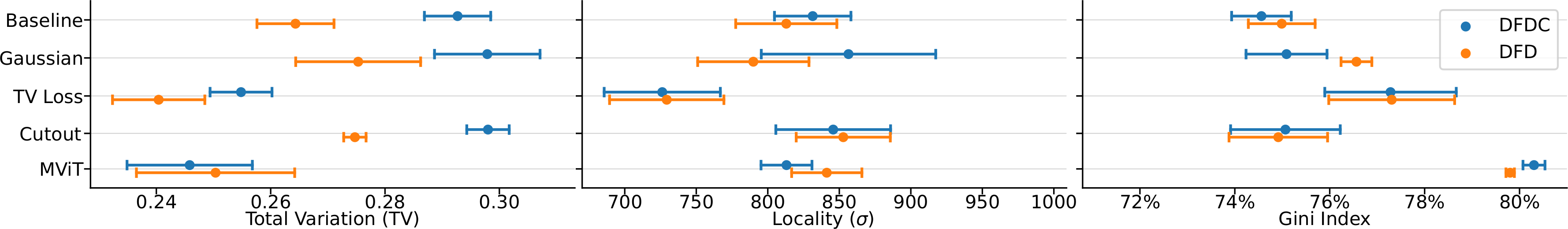
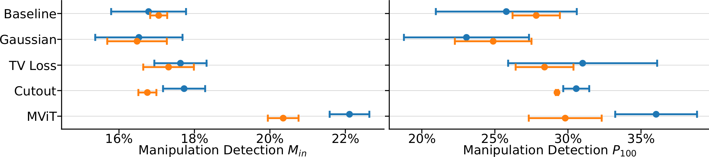
Figure 2: Quantitative explanation metrics: visual quality (top) and manipulation detection (bottom) for the evaluation subsets of DeepFake Detection Challenge (DFDC)and DeepFake Detection Dataset (DFD). Higher values indicate better explanation quality, except for TV and locality $\sigma$. Mean and standard deviation of 3 runs, full results in the appendix.

Data preparation.

As opposed to train-time augmentation, this term indicates transformations that are applied identically to all samples, e.gface detection and cropping described above. For image DeepFakes, Wang et alobserve that generated images have a weaker high-frequency content than real ones [Wang et al.(2021)Wang, Oramas, and Tuytelaars] and the explanations of models that rely on this clue are dominated by uninterpretable high-frequency noise. They suggest pre-processing all samples with a bilateral filter [Tomasi and Manduchi(1998)] to encourage focussing on other more interpretable features. In the same spirit, we investigate whether removing high-frequency video components improves smoothness and locality of the explanations in a quantifiable way.

Two variants are considered: a per-frame bilateral filter [Tomasi and Manduchi(1998)] or a spatio-temporal Gaussian filter; both configured so that common artefacts remain visible. Only training videos are filtered, leaving validation, test and explanation splits unaltered. As reported in  (Tab. 1), filtered videos result in lower classification performance, which corresponds to the observation in [Wang et al.(2021)Wang, Oramas, and Tuytelaars], and models trained with bilateral filtering fail to converge,thus we exclude them from explanation evaluation. Disappointingly, blurring does not seem to improve explanation metrics in a consistent way (Tab. 1), except for a slightly higher Gini Index that indicates sparser heatmaps. It is surely possible that stronger filters could produce more marked effects, but at the cost of lower classification performance. Otherwise, this outcome could be attributed to different generation techniques or compression formats between images and videos. Nevertheless, we recommend against this type of smoothing preprocessing [Wang et al.(2021)Wang, Oramas, and Tuytelaars] for video DeepFakes until proven more effective.

Regularization loss.

Regularization refers to training-time techniques that smooth or constrain the loss landscape so that the optimization process yields more desirable solutions that generalize better and/or yield better explanations. A common technique is to add a per-layer Total Variation (TV)term to the loss function during training [Rudin et al.(1992)Rudin, Osher, and Fatemi]. Considering the activation tensor $\bm{A}^{\ell}\in\mathbb{R}^{T\times H\times W}$ of an intermediate layer $\ell$, its anisotropic total variation is:

$$\mathcal{L}^{\ell}_{\text{TV}}=\frac{1}{THW}\sum_{d}\Omega_{\text{1D}}(\bm{A}^{\ell}_{d}),$$ (5)

where the summation considers all 1D slices of $\bm{A}$ orthogonal to its axes and $\Omega_{\text{1D}}$ indicates the 1D total variation. Averaging over all convolutional blocks in our architecture, the optimization objective results $\mathcal{L}=\mathcal{L}_{\text{task}}+\alpha\mathbb{E}_{\ell}\left[\mathcal{L}^{\ell}_{\text{TV}}\right]$, where $\alpha\in\mathbb{R}^{+}$ is a hyperparameter. The additional term places a smoothness constrain on the activations of intermediate layers, which we hope will result in localized peaks in the heatmap corresponding to visible artefacts in the video, though TV does not control the location of such peaks.

The first effect of TV regularization is noticeable during the initial phases of training. For unconstrained models, we observe that $\mathbb{E}_{\ell}\left[\mathcal{L}^{\ell}_{\text{TV}}\right]$ tends to increase during the initial phase of training and stabilizes at around $0.5$ after one epoch. On the other hand, when $\alpha=1$, the optimization process is dominated by $\mathcal{L}_{\text{TV}}$ for the first epochs and classification loss starts decreasing only after this term drops below $0.1$. From the results in Table 1, a strong TV regularization affects classification performance negatively. However, we also observe a significant improvement over the baseline for locality, sparsity, and manipulation in Figure 2. In fact, the average $\sigma$ for DFDC decreases from 814 to 726, indicating more spatially-focused explanations. Also, the Gini Index increases from 75% to 77%, meaning that fewer pixels are responsible for the bulk of the heatmaps. With respect to manipulation detection, the heatmaps produced by TV-regularized models match more closely the ground-truth, resulting in higher $P_{\text{100}}$ for both DFDC and DFD.

Video cutout.

Cutout data augmentation which can greatly improve classification performance by masking input patches at random during training [DeVries and Taylor(2017)]. We adapt Cutout to video data by replacing masking with heavy spatio-temporal blur: since motion blur occurs naturally, the augmented samples are maintained closer to the data manifold. We expect Facial Cutout to guide the network towards more meaningful representations, where the relationship between semantic parts of the face are better understood, hence improving part-based manipulation detection. On the other hand, removing parts of the input might yield more spread out heatmaps, as the network learns to capture information from more diverse locations. In our experiments, we observe slightly better generalization to DFD for regularized models (Table 1), which confirms the regularization properties of Facial Cutout. However, the effects on explanations are limited, resulting in slightly higher Total Variation and manipulation detection scores (Figure 2).

Architecture.

The architecture of a model represent a strong inductive biases on what features can be easily learned [Geirhos et al.(2018)Geirhos, Rubisch, Michaelis, Bethge, Wichmann, and Brendel, Tuli et al.(2021)Tuli, Dasgupta, Grant, and Griffiths]. As an alternative to the baseline S3D model, we consider another state-of-the-art architecture for video classification, namely a multi-scale vision transformer (MViT) [Fan et al.(2021)Fan, Xiong, Mangalam, Li, Yan, Malik, and Feichtenhofer]. The former, based on 3D convolutions, begins with forming local representations which are aggregated into more complex features in later layers. The latter, based on attention, allows all layers to attend to the input as a whole and encourages representation learning through progressive token aggregation. We expect the different inductive biases and information flow to affect the explanation heatmaps generated by these architectures. In particular, we fine-tune the MViT-B $16\times 4$ variant with the default hyperparameters: random color augmentation, temporal subsampling, cosine learning rate annealing, and weight initialization from Kinetics 400. For ease of comparison, MViT explanations are obtained with SmoothGrad while attention-specific methods are left to future work.

For the classification task, MViT achieves the best performance on the two datasets (Tab. 1), which we attribute to the longer training cycle. The explanation heatmaps obtained with this architecture are also significantly smoother (TV) and sparser (Gini Index) than CNN-based models, while spatial locality remains similar ($\sigma$). Furthermore, the bottom row of Fig. 2 indicates that MViT heatmaps are stronger detectors of manipulated areas, focusing most of the heatmap inside the ground-truth mask ($M_{\text{in}}$). We attribute these promising results to i) a more robust classifier which can better distinguish fake videos and is thus likely to have learned a good representation of manipulation artefacts ii) the underlying inductive bias of attention and its effect on gradient propagation used for heatmap generation

4.2 Communicating explanations

As discussed, gradient-based explanations often appear too noisy for users to easily parse. We propose four simple techniques to post-process heatmaps into increasingly more structured visualizations i) enhanced heatmaps, clip extreme values and smooth to eliminate high-frequency noise ii) gaussian matching, draw an ellipse corresponding to the mean and variance of each frame iii) blob detection, run a DoG blob detector [Collins(2003), Pedregosa et al.(2011)Pedregosa, Varoquaux, Gramfort, Michel, Thirion, Grisel, Blondel, Prettenhofer, Weiss, Dubourg, Vanderplas, Passos, Cournapeau, Brucher, Perrot, and Duchesnay] and highlight each blob according to its relevance iv) semantic aggregation, aggregate the heatmap into semantic regions and highlight each part based on its relevance

A small-scale user study (34 participants) is carried out to quantify user satisfaction with respect to each of these visualization techniques. Each user is presented a set of 10 videos as in Fig. 3(a) and is asked to rate the four visualizations, which appear in random order. A score of 0 means that the visualization is not helpful to detect the DeepFake, while 5 means it easily allowed for its detection. To minimize appreciation bias, ratings are centered per-user before aggregation by subtracting the average score. From the results in Fig. 3(b) we observe a clear relationship between user satisfaction and more structured visualizations. However, when the classifier performs poorly and heatmaps are uninformative, users will be dissatisfied regardless of post-processing. However, we also note that when the classifier performs poorly, users will be generally dissatisfied.

(a) From left to right: real video, fake video, enhanced heatmap, Gaussian matching, blob detection, semantic aggregation.

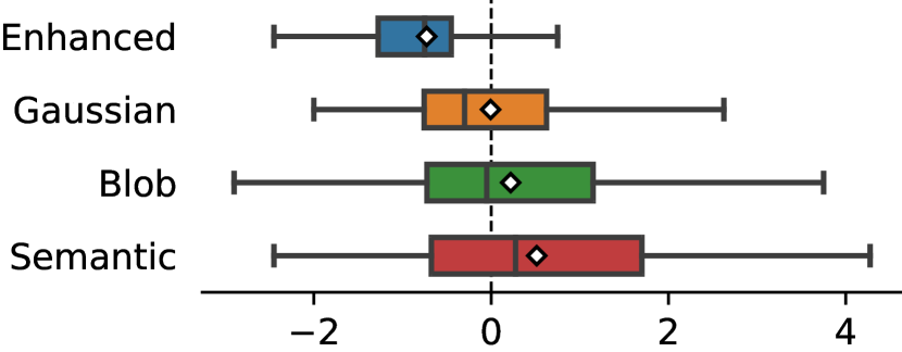
(b) User ratings for alternative explanation visualizations.

Figure 3: User study. Left panel: an example of the visualizations submitted to human observation for the study. Right panel: box plot of normalized score for each explanation visualization technique which semantic aggregation as preferred.

5 Conclusion

The Explainable AI has developed a plethora of explanation methods of varying degrees of faithfulness. However, to the best of our knowledge, quantitative metrics to compare the quality of such explanations are lacking. This work attempts to lay out an objective evaluation framework for DeepFake explanations, which we hope will drive the development of detectors that are better aligned with human cognition. The main contribution of this paper is the introduction of a family of such metrics, novel or adapted from existing works, to measure visual quality and manipulation detection.

In our experiments we consider several techniques for training DeepFake detectors and study their impact on explainability metrics in a quantitative way, whereas previous work was limited to qualitative comparisons. We observe that TV regularization has the largest impact across most metrics. On the other hand, controlling high-frequency components of the input is of little utility, at least when realistic video compression settings are considered. Finally, we observe that recent architectures such as MViT significantly outperform any of the S3D variations in both detection and explanation quality. We recommend further study of transformer-based DeepFake classifiers and how to employ attention as an explanation.

Ethical statement.

As DeepFake technology becomes increasingly accessible, so is the potential for malicious use. It is therefore urgent to present society with the necessary tools to address this problem and facilitate the safe and ethical use of these creations. We believe this line of work can bring positive societal impact by facilitating good governance and wider adoption of DeepFake detectors across all media. Furthermore, more explainable DeepFake detectors can be used to educate the public to better distinguish between real and generated content. From their perspective, users must feel confident about the technologies that routinely affects their interactions, which may otherwise fall victim to mistrust.

Limitations and future work.

This project leads to many natural avenues for future research in Explainable AI. First, although the proposed metrics are drawn from existing literature and are based on sound mathematical foundations, an extensive study of the correlation between these metrics and human preference would increase their reliability. Second, it is surely possible to conceive more refined metrics for DeepFake detection to address the shortcomings discussed in Section 3.2. For instance, we have already mentioned that locality ($\sigma$) favors unimodal over multimodal heatmaps, whereas more faceted metrics of localization are desirable. Third, as made evident from the experiments on DeepFake Dataset, when classification performance is not perfect explanations can be meaningless. Thus, combining explanations and uncertainty estimation would provide a more complete picture of any DeepFake detector. Finally, we remark that the proposed metrics are not meant to supplant human judgment, e.guser studies, but rather to provide a non-interactive and repeatable benchmark that is more suitable for guiding the development and facilitating the deployment of better DeepFake detectors.

Supplementary Material

Appendix A Datasets

A.1 DeepFake Detection Challenge

The DFDC dataset was released as part of the homonymous Kaggle challenge [Dolhansky et al.(2020)Dolhansky, Bitton, Pflaum, Lu, Howes, Wang, and Ferrer]. It contains approximately 120k videos, the majority of which are DeepFakes created with different manipulation methods. The dataset comes in different variants of compression quality, which are mostly relevant for training robust classifiers and assessing detection performance. For an analysis of explanation quality, we choose to work on high-quality videos where we expect manipulation artifacts to be more prominent. Table 2 reports how many videos are used for training, validation, testing and explanation evaluation.

Preprocessing.

The videos from the dataset might contain one or more faces. Of these, only one is manipulated in the case of “fake” videos. For the purpose of training the DeepFakes classifier, each video is preprocessed as follows:

1. Videos are spatially resized with padding so that each frame is $640\times 640$ pixels;

2. MTCNN is applied every 5 frames, which outputs rectangular bounding boxes tightly cropped around all faces in a frame

3. Face detections are linked across frames using a greedy overlap-based heuristic; namely, if two bounding boxes overlap with $\text{IoU}>0.5$ they are considered the same face;

4. The longest consecutive sequence of linked boxes is considered the main face and is assumed to be the target for DeepFake manipulation, all other boxes are discarded and the video is clipped to the frames containing the main face;

5. For intermediate frames where MTCNN was not applied, a bounding box for the main face is created by linearly interpolating the corners of the two closest boxes;

6. Boxes are expanded by $1.5\times$ to capture more of the hair, neck and background

7. All frames belonging to the main face sequence are cropped according to their box; rectangular crops are resized to $224\times 224$ and used for training;

8. BiSeNet is applied every 5th frame of a $512\times 512$ version of the aforementioned video, the probabilistic output of BiSeNet is resized with bilinear interpolation to match the original size and then the most likely face part is selected.

Classification.

For training, validation, and testing, each video is processed separately. This means that fake videos will not be perfectly aligned with the corresponding real video, neither in space nor in time. Also, it means that detection and parsing might fail on some fake videos, due to the low quality of the manipulation. While this can hinder training, it also represents a realistic scenario where unseen videos are submitted to a trained classifier.

Expalantion evaluation.

Explanation metrics based on manipulation detection require perfectly-aligned pairs of real-fake videos. Therefore, face detection and parsing are performed on real videos and applied identically to all corresponding fake videos. Since the pairing between real and manipulated videos is only given for the training split of DeepFake Detection Challenge, and only some videos are perfectly aligned, we use an held-out subset of the training split consisting of 230 fake videos created from 100 real videos.

A.2 DeepFake Detection Dataset

The DeepFake Detection Dataset [Nick Dufour and Andrew Gully(2019)] is constructed by recording actors in various situations and then applying face-swapping DeepFake techniques to the videos. The dataset contains a large number of videos, but only a limited number of them are perfectly aligned and can be used for evaluating explanations on part-based manipulation detection. With respect to the classification task, this dataset is never used during training and it represents a good benchmark for out-of-distribution generalization. Table 2 reports the number of videos used to evaluate classification performance and explanation metrics. The videos are preprocessed in the same way as DFDC. For manipulation detection, perfect alignment is available for 107 fake videos created from 37 real ones.

Table 2: Dataset sizes: number of real and fake videos contained in each dataset and split. DFDC is used to train all classifiers in this work, to report classification metrics, and to evaluate explanation metrics. DFD is only used for testing and explanation evaluation.

	DFDC		DFD
	Real	Fake	Real	Fake
Train	19143	99953	-	-
Validation	1975	1968	-	-
Test	2479	2486	37	107
Explanation	100	230	37	107

Appendix B Classification performance

We report relevant classification metrics for the test split of DFDC in Table 3 and for a subset of DFD in Table 4. In addition to cross-entropy loss ($\mathcal{L}_{\text{CE}}$) and area under the receiver operating characteristic curve ($A_{\text{ROC}}$), we also report precision, recall, and F1 scores obtained when the model output is binarized with a threshold of 0.5. Furthermore, we report average precision (AP), i.ethe area under the precision-recall curve as the classification threshold changes. For each metric and configuration described in Section 3.2 and Section 4, we report mean and standard deviation of 3 runs.

Table 3: Classification metrics for DFDC, test split. For each configuration and metric, mean and standard deviation of 3 runs are reported. For all metrics except the $\mathcal{L}_{\text{CE}}$ loss, values are given in percentage and a higher value indicates a better result.

	$\mathcal{L}_{\text{CE}}\downarrow$		Precision $\uparrow$		Recall $\uparrow$		F1 $\uparrow$		AP $\uparrow$		$A_{\text{ROC}}\uparrow$
	avg	std	avg	std	avg	std	avg	std	avg	std	avg	std
S3D Baseline	0.447	0.036	80.89	1.82	82.27	4.01	81.50	1.17	88.79	2.19	89.02	1.08
S3D Bilateral	0.696	0.003	54.00	0.15	32.06	8.47	39.91	6.74	52.75	0.58	54.24	0.67
S3D Gaussian	0.542	0.031	78.49	1.51	64.26	2.89	70.65	2.16	80.20	3.30	81.77	2.33
S3D TV Loss	0.460	0.027	78.68	1.53	81.04	3.50	79.82	2.12	88.24	1.78	87.41	1.88
S3D Cutout	0.481	0.037	78.39	0.73	82.72	4.10	80.46	1.87	86.42	3.56	87.19	2.14
MViT	0.430	0.004	83.64	0.28	94.30	1.46	88.65	0.57	96.59	0.32	96.38	0.38

Table 4: Classification metrics for DFD. For each configuration and metric, mean and standard deviation of 3 runs are reported. For all metrics except the $\mathcal{L}_{\text{CE}}$ loss, values are given in percentage and a higher value indicates a better result.

	$\mathcal{L}_{\text{CE}}\downarrow$		Precision $\uparrow$		Recall $\uparrow$		F1 $\uparrow$		AP $\uparrow$		$A_{\text{ROC}}\uparrow$
	avg	std	avg	std	avg	std	avg	std	avg	std	avg	std
S3D Baseline	0.694	0.080	72.48	5.55	61.64	2.81	66.59	3.73	82.88	2.67	80.24	2.31
S3D Bilateral	0.746	0.006	42.37	0.56	26.97	2.51	32.94	2.05	43.90	0.00	45.82	0.29
S3D Gaussian	0.760	0.055	60.51	1.77	49.03	12.73	53.66	8.34	66.03	2.37	66.42	0.90
S3D TV Loss	0.698	0.038	65.21	2.03	66.79	7.17	65.90	4.25	77.66	3.72	75.75	3.59
S3D Cutout	0.655	0.065	72.48	5.26	59.95	4.25	65.44	1.97	82.23	0.91	79.59	0.48
MViT	0.513	0.015	74.75	1.24	83.41	3.50	78.83	2.12	91.73	1.70	90.04	1.79

Appendix C Training details

C.1 High-frequencies smoothing

For models trained with smoothing preprocessing, either Gaussian blur or bilateral filtering are applied. Gaussian blur is applied at the video level using a spatial standard deviation of 0.8 and a temporal standard deviation of 0.5. Bilateral filtering is applied per-frame using a spatial standard deviation of 2 and a color range standard deviation of 0.1. These values are empirically chosen so that the filtered videos remain qualitatively similar to the original ones and that common DeepFake artefacts are still visible.

C.2 Default video augmentation

For all models, color augmentations are applied to training videos to improve generalization. Each video is augmented with probability 0.5. If the video is augmented, one of the following transformations is chosen with equal probability: grayscale conversion, RGB shifting, gamma shifting, contrast limited adaptive histogram equalization, hue, saturation and value shifting, brightness and contrast shifting.

C.3 Cutout

When cutout is enabled, each video is augmented with cutout with probability 0.5. Cutout acts on a $64\times 64$ region of the video selected with uniform probability. Once a mask is selected, its contents are blurred with a strong Gaussian filter (standard deviation 4).

C.4 Architectures and training details

Multiscale S3D.

The S3D architecture consists of several inception blocks using separable 3D convolution layers. We use a model pretrained on Kinetics 400 as the backbone feature extractor for the DeepFake classifier. On top of the original architecture, we add shortcut connections from intermediate layers to the classification head,to allow easier access to multiscale features which might be relevant for the task. Specifically, we collect the input activations of the 2nd, 3rd, 4th and 5th pooling layers. These activations are first average-pooled to the size of the smallest one, concatenated, processed through $1\times 1\times 1$ convolution, and eventually pooled into a 128-dimensional feature vector. The classification head is a simple 2-layer MLP with output size of 2 and softmax activation.

During one epoch of training, real videos are sampled more than once to match the number of fake videos in the training set. From each video, a clip of 64 consecutive frames is extracted at random. Videos shorter than 64 frames are padded by appending black frames. No spatial cropping is performed since the videos already contain centered faces. The optimizer processes mini-batches of 32 videos at the time. The learning rate of the Adam optimizer is set to $10^{-4}$ for pretrained parameters and to $10^{-3}$ for the classification head. An additional weight decay loss is applied to all parameters except biases with strength $10^{-5}$.

For validation, only the first 64 frames of each video are considered and no augmentations are applied. Training runs for 5 epochs, unless validation loss stops decreasing, in which case early stopping is applied. The results reported in the tables are relative for videos in the training set. For these, we average the output probabilities of 5 equally-spaced 64-frames clips from each video.

Multiscale ViT.

As an alternative to the 3D CNN backbone, we experiment with a transformer architecture. Specifically, we use a Multiscale Vision Transformer that combines attention layers with multiscale hierarchical processing. For this model, we maintain the original architecture except for the classification head that is modified to output 2 classes. Similarly to S3D, the weights are initialized from a model pretrained on Kinetics 400.

Training, validation and testing follow the default settings from the authors. Namely, the learning rate follows a cosine annealing schedule without warm-up, random temporal crops of 16 frames are selected from each training video, multiple temporal crops are considered for testing, spatial cropping is disabled.

Compute resources.

All models are trained on a single machine equipped with 4 NVIDIA V100 GPUs with 32GB of RAM each, which allow for large batch sizes. Once trained, the model can be ran for both inference and explanations on more modest hardware, e.ga single GPU environment with 12GB of RAM.

Appendix D Explanation metrics

This section details how the explanation metrics introduced in Section 3.2 are computed in practice using discretized videos, masks and heatmaps. Furthermore, Table 5 and Table 6 report the metrics for all variations considered in this work as the average and standard deviation of 3 runs each.

The main text uses a compact notation where videos are defined as a mapping from the discretized grid $\mathcal{G}=\{1,\ldots,T\}\times\{1,\ldots,H\}\times\{1,\ldots,W\}$ to RGB pixel values. For this appendix, we choose a more explicit notation based on tensors. We remark the equivalence between the two notations since any function $f:\mathcal{G}\rightarrow R^{+}$ can be uniquely represented as a $T\!\times\!H\!\times\!W$ tensor whose element at $(t,h,w)$ is $f(t,h,w)$. In this context, it is useful to define the derivative and integral operators $\nabla$ and $\int$ as:

$$\left(\nabla f(\bm{\rho})\right)_{i=1,2,3} =f(\bm{\rho}+\bm{e}_{i})-f(\bm{\rho}),$$ (6)

$$\int_{\mathcal{G}}fd\lambda =\frac{1}{THW}\sum_{\bm{\rho}\in\mathcal{G}}f(\bm{\rho}),$$ (7)

where the vector $\bm{\rho}=(t,u,v)$ denotes the pixel coordinates, and the vectors $\bm{e}_{i}$ are the usual orthonormal basis i.e. $(e_{i})_{j}=\delta_{ij}$.

D.1 Total variation

Total variation is used to measure the smoothness of a heatmap and is defined as:

$$\operatorname{TV}(h)=\frac{1}{THW}\sum_{\bm{\rho}\in\mathcal{G}}\nabla h(\bm{\rho}),$$ (8)

where the discrete gradient $\nabla h$ at coordinates $\bm{\rho}=(t,u,v)$ is computed as:

$$\left|h(t,u,v)-h(t+1,u,v)\right|+\left|h(t,u,v)-h(t,u+1,v)\right|+\left|h(t,u,v)-h(t,u,v+1)\right|$$ (9)

D.2 Variance volume

To measure the spatial localization of the heatmap, we first compute its mean and variance:

$$\bm{\mu} =\sum_{\bm{\rho}\in\mathcal{G}}\bm{\rho}h(\bm{\rho}),$$ (10)

$$\bm{\Sigma} =\sum_{\bm{\rho}\in\mathcal{G}}(\bm{\rho}-\bm{\mu})(\bm{\rho}-\bm{\mu})^{T}h(\bm{\rho}),$$ (11)

where the vector $\bm{\rho}=(t,u,v)^{T}$ represents pixel coordinates. Then, to summarize the $3\times 3$ variance matrix as a scalar, we consider its volume given by the determinant $|\det(\bm{\Sigma})|$. Larger volumes correspond to more spread out heatmaps, while smaller values indicate more localized explanations. Importantly, this metric is particularly indicated for unimodal heatmaps that focus around a single location of the video.

D.3 Gini Index

The Gini Index was initially introduced as an economic indicator of wealth distribution [Gini(1912)], but it is considered a good measure of sparsity due to its properties [Hurley and Rickard(2009)]. The Gini Index of an heatmap measures is defined as:

$$\operatorname{G}=\frac{2}{THW}\frac{\sum_{i}i\cdot h(\bm{\rho_{i}})}{\sum_{i}h(\bm{\rho_{i}})}-\frac{THW+1}{THW},$$ (12)

with the indices $i=1,\ldots,THW$ that select pixel coordinates such that $h(\bm{\rho}_{i})\leq h(\bm{\rho}_{i+1})$. Notably, the “sparsity” measured by the Gini Index refers to the scalar importance values of each pixel and not their location in the heatmap. The heatmap will have a high Gini Index if most of the explanation mass is concentrated in few highly-relevant pixels while all other pixels have low relevance.

D.4 Faithfulness

Faithfulness is generally used to compare explanation methods on the basis of how closely they identify portions of the input that are meaningful for the classifier and a particular decision. Faithfulness is measured using the deletion score, which represents the area under the curve traced by the confidence in $p(\textsc{fake}|v)$ as pixels are removed from the video in decreasing order of relevance. Considering the large amount of pixels in a video, the curve is approximated by removing several pixels in one step. Specifically, we consider the sorted values of an heatmap $h$ and group them in 25 bins. These bins do not necessarily contain the same amount of pixels, but the total relevance in each bin is approximately the same.

In this work, we are interested in the properties of explanations rather than of explanation methods. However, a faithful explanation method is a prerequisite for further evaluation of explanation quality. As a preliminary step, we compare the four explanation methods discussed in Sec. 3.1 and choose the most faithful one based on its deletion scores on the baseline model. The following hyperparameters are used: in SmoothGrad, gradients are averaged over 25 randomly perturbed videos with a noise parameter equal to 0.15 of the RGB range; in Integrated Gradients the path integral is calculated w.r.ta black video baseline using 25 interpolation steps.

With respect to fake videos in DFDC and DFD, the four methods achieve the following average deletion scores: Sensitivity 42.54%, Gradient$\times$Input 43.68%, SmoothGrad 41.25%, Integrated Gradients 43.77%. Therefore, SmoothGrad has the lowest deletion score of the four (p value of paired one-sided t-test $<10^{-5}$) and is then employed throughout all experiments.

D.5 Manipulation detection

The ability to detect and localize manipulations is measured by considering videos created by overlaying a portion of a fake video $v_{F}$ to its corresponding original video $v_{R}$. The blending mask is obtained by selecting a face part $p\in\{\text{mouth},\text{nose},\text{eyes}\}$ from those extracted with BiSeNet [Yu et al.(2021)Yu, Gao, Wang, Yu, Shen, and Sang]. The explanation heatmap can then be compared with the ground-truth manipulation mask to determine whether the model is focusing on manipulated regions of the video. Without loss of generality, only the first 64 frames of each video are considered in all manipulation detection evaluations.

For the main metrics, we measure the precision of 100 most-relevant pixels in the heatmap, and the percentage of heatmap contained in the ground-truth manipulation mask. This approach has the advantage of being threshold independent, as opposed to binarizing the heatmap using an arbitrary threshold and computing metrics such as Intersection over Union. Notably, both metrics penalize explanations that focus outside the ground-truth mask, but can not distinguish whether the heatmap clusters around an actual manipulation artefact or is uniformly scattered inside the mask (Figure 6).

Table 5: Explanation metrics for DeepFake Detection Challenge (DFDC). Mean and standard deviation of 3 independent classifiers whose decisions are explained using SmoothGrad.

	TV $\downarrow$		$\sqrt[3]{\sigma}\downarrow$		Gini $\uparrow$		$M_{\text{IN}}\uparrow$		$P_{100}\uparrow$
	avg	std	avg	std	avg	std	avg	std	avg	std
S3D Baseline	0.285	0.006	814.4	31.0	74.93	1.00	17.43	0.38	29.43	1.34
S3D Bilateral	0.428	0.044	1372.6	268.8	67.89	3.50	12.15	3.32	13.47	8.77
S3D Gaussian	0.292	0.004	841.4	15.1	75.55	0.44	17.38	0.51	26.31	1.19
S3D TV Loss	0.256	0.003	726.3	54.8	77.40	1.97	17.68	1.00	34.46	1.85
S3D Cutout	0.296	0.005	839.0	40.2	75.26	1.40	17.76	0.63	30.48	1.10
MViT	0.246	0.013	808.3	17.1	80.42	0.36	22.11	0.64	36.03	3.43

Table 6: Explanation metrics for DeepFake Detection Dataset (DFD). Mean and standard deviation of 3 independent classifiers whose decisions are explained using SmoothGrad.

	TV $\downarrow$		$\sqrt[3]{\sigma}\downarrow$		Gini $\uparrow$		$M_{\text{IN}}\uparrow$		$P_{100}\uparrow$
	avg	std	avg	std	avg	std	avg	std	avg	std
S3D Baseline	0.261	0.009	827.6	34.4	74.84	0.74	17.09	0.15	28.62	0.80
S3D Bilateral	0.413	0.061	1426.3	346.3	68.92	4.95	13.47	4.25	16.10	16.48
S3D Gaussian	0.273	0.011	799.2	11.0	76.54	0.17	16.83	0.82	26.87	1.16
S3D TV Loss	0.244	0.005	742.1	45.3	77.08	1.70	17.20	0.92	30.09	2.72
S3D Cutout	0.274	0.004	838.7	46.5	75.33	1.47	16.87	0.31	29.22	0.96
MViT	0.250	0.016	834.5	27.3	80.02	0.10	20.35	0.50	29.81	3.06

Appendix E Additional examples

Additional examples of semantic parsing, manipulation detection (Section 3.2.2), and explanation post-processing for the user study (Section 4.2) are shown below.

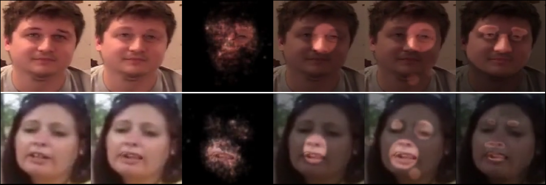
Figure 4: User study visualization: real video, fake video, enhanced heat-map, Gaussian matching, blob detection, semantic aggregation.

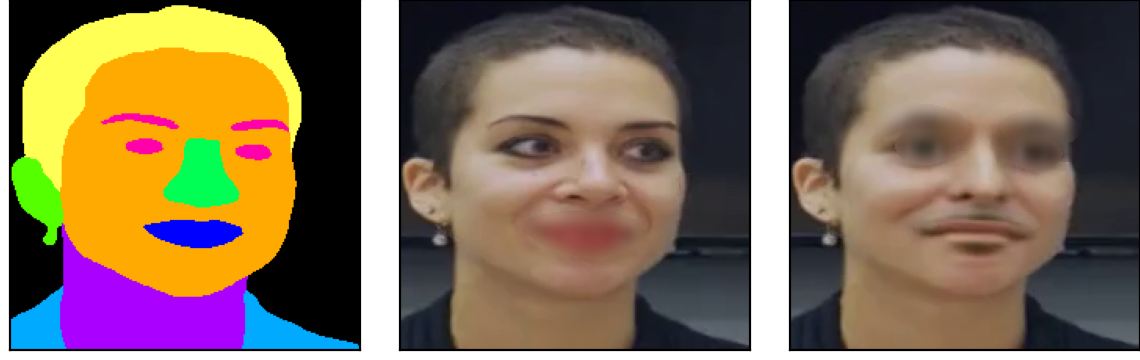
Figure 5: Example of semantic parsing as performed by BiSeNet [Yu et al.(2021)Yu, Gao, Wang, Yu, Shen, and Sang] and of an alternative version of video cutout (Section 3.2.2) where heavy blurring is applied dynamically to a semantic region instead of a fixed square.

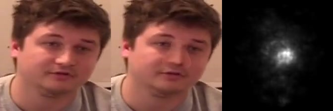
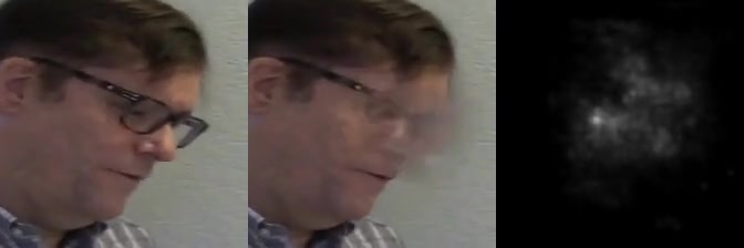
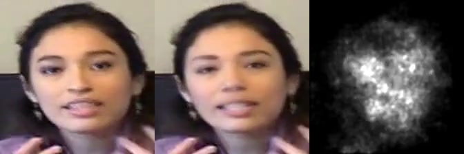
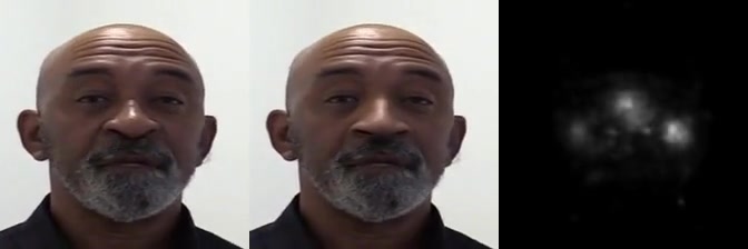
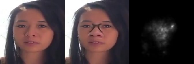
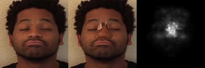
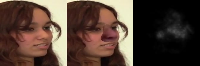
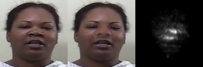
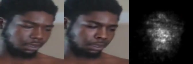
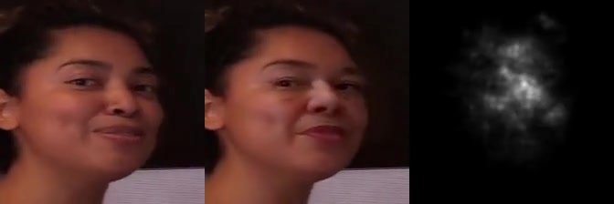
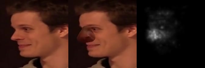
Figure 6: Additional examples for manipulation detection. Random frames from random videos. From left to right: original, part-based manipulated video, heatmap.

References

- [Abnar and Zuidema(2020)] Samira Abnar and Willem Zuidema. Quantifying Attention Flow in Transformers. In Proceedings of the 58th Annual Meeting of the Association for Computational Linguistics, pages 4190–4197, Online, July 2020. Association for Computational Linguistics. 10.18653/v1/2020.acl-main.385.
- [Afchar et al.(2018)Afchar, Nozick, Yamagishi, and Echizen] Darius Afchar, Vincent Nozick, Junichi Yamagishi, and Isao Echizen. Mesonet: A compact facial video forgery detection network. In 2018 IEEE International Workshop on Information Forensics and Security (WIFS), pages 1–7. IEEE, 2018.
- [Agarwal et al.(2019)Agarwal, Farid, Gu, He, Nagano, and Li] Shruti Agarwal, Hany Farid, Yuming Gu, Mingming He, Koki Nagano, and Hao Li. Protecting World Leaders Against Deep Fakes. In IEEE Conference on Computer Vision and Pattern Recognition Workshops (CVPRW), volume 1, 2019.
- [Alvarez Melis and Jaakkola(2018)] David Alvarez Melis and Tommi Jaakkola. Towards Robust Interpretability with Self-Explaining Neural Networks. Advances in Neural Information Processing Systems, 31, 2018.
- [Amerini et al.(2019)Amerini, Galteri, Caldelli, and Del Bimbo] Irene Amerini, Leonardo Galteri, Roberto Caldelli, and Alberto Del Bimbo. Deepfake Video Detection through Optical Flow Based CNN. In Proceedings of the IEEE/CVF International Conference on Computer Vision Workshops, pages 0–0, 2019.
- [Ancona et al.(2018)Ancona, Ceolini, Öztireli, and Gross] Marco Ancona, Enea Ceolini, Cengiz Öztireli, and Markus Gross. Towards better understanding of gradient-based attribution methods for Deep Neural Networks. In International Conference on Learning Representations, February 2018.
- [Arnab et al.(2021)Arnab, Dehghani, Heigold, Sun, Lučić, and Schmid] Anurag Arnab, Mostafa Dehghani, Georg Heigold, Chen Sun, Mario Lučić, and Cordelia Schmid. ViViT: A Video Vision Transformer. arXiv:2103.15691 [cs], March 2021.
- [Bach et al.(2015)Bach, Binder, Montavon, Klauschen, Müller, and Samek] Sebastian Bach, Alexander Binder, Grégoire Montavon, Frederick Klauschen, Klaus-Robert Müller, and Wojciech Samek. On Pixel-Wise Explanations for Non-Linear Classifier Decisions by Layer-Wise Relevance Propagation. PLOS ONE, 10(7):e0130140, July 2015. ISSN 1932-6203. 10.1371/journal.pone.0130140.
- [Baldassarre et al.(2020)Baldassarre, Smith, Sullivan, and Azizpour] Federico Baldassarre, Kevin Smith, Josephine Sullivan, and Hossein Azizpour. Explanation-Based Weakly-Supervised Learning of Visual Relations with Graph Networks. In Andrea Vedaldi, Horst Bischof, Thomas Brox, and Jan-Michael Frahm, editors, ECCV 2020, Lecture Notes in Computer Science, pages 612–630. Springer International Publishing, 2020. ISBN 978-3-030-58604-1. 10.1007/978-3-030-58604-1_37.
- [Barredo Arrieta et al.(2020)Barredo Arrieta, Díaz-Rodríguez, Del Ser, Bennetot, Tabik, Barbado, Garcia, Gil-Lopez, Molina, Benjamins, Chatila, and Herrera] Alejandro Barredo Arrieta, Natalia Díaz-Rodríguez, Javier Del Ser, Adrien Bennetot, Siham Tabik, Alberto Barbado, Salvador Garcia, Sergio Gil-Lopez, Daniel Molina, Richard Benjamins, Raja Chatila, and Francisco Herrera. Explainable Artificial Intelligence (XAI): Concepts, taxonomies, opportunities and challenges toward responsible AI. Information Fusion, 58:82–115, June 2020. ISSN 1566-2535. 10.1016/j.inffus.2019.12.012.
- [Bondi et al.(2020)Bondi, Daniele Cannas, Bestagini, and Tubaro] Luca Bondi, Edoardo Daniele Cannas, Paolo Bestagini, and Stefano Tubaro. Training Strategies and Data Augmentations in CNN-based DeepFake Video Detection. In 2020 IEEE International Workshop on Information Forensics and Security (WIFS), pages 1–6, December 2020. 10.1109/WIFS49906.2020.9360901.
- [Bonettini et al.(2021)Bonettini, Cannas, Mandelli, Bondi, Bestagini, and Tubaro] Nicolò Bonettini, Edoardo Daniele Cannas, Sara Mandelli, Luca Bondi, Paolo Bestagini, and Stefano Tubaro. Video Face Manipulation Detection Through Ensemble of CNNs. In 2020 25th International Conference on Pattern Recognition (ICPR), pages 5012–5019, January 2021. 10.1109/ICPR48806.2021.9412711.
- [Cao et al.(2015)Cao, Liu, Yang, Yu, Wang, Wang, Huang, Wang, Huang, Xu, Ramanan, and Huang] Chunshui Cao, Xianming Liu, Yi Yang, Yinan Yu, Jiang Wang, Zilei Wang, Yongzhen Huang, Liang Wang, Chang Huang, Wei Xu, Deva Ramanan, and Thomas S. Huang. Look and Think Twice: Capturing Top-Down Visual Attention with Feedback Convolutional Neural Networks. In 2015 IEEE International Conference on Computer Vision (ICCV), pages 2956–2964, December 2015. 10.1109/ICCV.2015.338.
- [Chefer et al.(2021)Chefer, Gur, and Wolf] Hila Chefer, Shir Gur, and Lior Wolf. Generic Attention-Model Explainability for Interpreting Bi-Modal and Encoder-Decoder Transformers. In arXiv:2103.15679 [Cs], March 2021.
- [Coccomini et al.(2021)Coccomini, Messina, Gennaro, and Falchi] Davide Coccomini, Nicola Messina, Claudio Gennaro, and Fabrizio Falchi. Combining EfficientNet and Vision Transformers for Video Deepfake Detection. arXiv:2107.02612 [cs], July 2021.
- [Collins(2003)] Robert T. Collins. Mean-shift blob tracking through scale space. In 2003 IEEE Computer Society Conference on Computer Vision and Pattern Recognition, 2003. Proceedings., volume 2, pages II–234. IEEE, 2003.
- [Damiani(2019)] Jesse Damiani. A Voice Deepfake Was Used To Scam A CEO Out Of $243,000. https://www.forbes.com/sites/jessedamiani/2019/09/03/a-voice-deepfake-was-used-to-scam-a-ceo-out-of-243000/, September 2019.
- [Dang et al.(2020)Dang, Liu, Stehouwer, Liu, and Jain] Hao Dang, Feng Liu, Joel Stehouwer, Xiaoming Liu, and Anil K. Jain. On the detection of digital face manipulation. In Proceedings of the IEEE/CVF Conference on Computer Vision and Pattern Recognition, pages 5781–5790, 2020.
- [Deepfakes Team(2021)] Deepfakes Team. Deepfakes, November 2021.
- [DeVries and Taylor(2017)] Terrance DeVries and Graham W. Taylor. Improved Regularization of Convolutional Neural Networks with Cutout. arXiv:1708.04552 [cs], November 2017.
- [Dolhansky et al.(2020)Dolhansky, Bitton, Pflaum, Lu, Howes, Wang, and Ferrer] Brian Dolhansky, Joanna Bitton, Ben Pflaum, Jikuo Lu, Russ Howes, Menglin Wang, and Cristian Canton Ferrer. The DeepFake Detection Challenge (DFDC) Dataset. arXiv:2006.07397 [cs], October 2020.
- [Dosovitskiy et al.(2020)Dosovitskiy, Beyer, Kolesnikov, Weissenborn, Zhai, Unterthiner, Dehghani, Minderer, Heigold, Gelly, Uszkoreit, and Houlsby] Alexey Dosovitskiy, Lucas Beyer, Alexander Kolesnikov, Dirk Weissenborn, Xiaohua Zhai, Thomas Unterthiner, Mostafa Dehghani, Matthias Minderer, Georg Heigold, Sylvain Gelly, Jakob Uszkoreit, and Neil Houlsby. An Image is Worth 16x16 Words: Transformers for Image Recognition at Scale. In arXiv:2010.11929 [Cs], September 2020.
- [European Union(2018)] European Union. General Data Protection Regulation (GDPR). https://gdpr.eu/, 2018.
- [Fan et al.(2021)Fan, Xiong, Mangalam, Li, Yan, Malik, and Feichtenhofer] Haoqi Fan, Bo Xiong, Karttikeya Mangalam, Yanghao Li, Zhicheng Yan, Jitendra Malik, and Christoph Feichtenhofer. Multiscale Vision Transformers. arXiv:2104.11227 [cs], April 2021.
- [Fong and Vedaldi(2017)] Ruth C. Fong and Andrea Vedaldi. Interpretable Explanations of Black Boxes by Meaningful Perturbation. In 2017 IEEE International Conference on Computer Vision (ICCV), pages 3449–3457, Venice, October 2017. IEEE. ISBN 978-1-5386-1032-9. 10.1109/ICCV.2017.371.
- [Geirhos et al.(2018)Geirhos, Rubisch, Michaelis, Bethge, Wichmann, and Brendel] Robert Geirhos, Patricia Rubisch, Claudio Michaelis, Matthias Bethge, Felix A. Wichmann, and Wieland Brendel. ImageNet-trained CNNs are biased towards texture; increasing shape bias improves accuracy and robustness. In International Conference on Learning Representations, September 2018.
- [Generated Photos Team(2018)] Generated Photos Team. Generated Photos Dataset. https: //generated.photos/, 2018.
- [Gilpin et al.(2018)Gilpin, Bau, Yuan, Bajwa, Specter, and Kagal] Leilani H. Gilpin, David Bau, Ben Z. Yuan, Ayesha Bajwa, Michael Specter, and Lalana Kagal. Explaining Explanations: An Overview of Interpretability of Machine Learning. The 5th IEEE International Conference on Data Science and Advanced Analytics (DSAA 2018)., June 2018.
- [Gini(1912)] Corrado Gini. Variabilità e mutabilità: contributo allo studio delle distribuzioni e delle relazioni statistiche. Tipogr. di P. Cuppini, 1912.
- [Güera and Delp(2018)] David Güera and Edward J. Delp. Deepfake Video Detection Using Recurrent Neural Networks. In 2018 15th IEEE International Conference on Advanced Video and Signal Based Surveillance (AVSS), pages 1–6, November 2018. 10.1109/AVSS.2018.8639163.
- [Hurley and Rickard(2009)] Niall Hurley and Scott Rickard. Comparing Measures of Sparsity. IEEE Transactions on Information Theory, 55(10):4723–4741, October 2009. ISSN 1557-9654. 10.1109/TIT.2009.2027527.
- [Jain and Wallace(2019)] Sarthak Jain and Byron C. Wallace. Attention is not Explanation. In Proceedings of the 2019 Conference of the North American Chapter of the Association for Computational Linguistics: Human Language Technologies, Volume 1 (Long and Short Papers), pages 3543–3556, Minneapolis, Minnesota, June 2019. Association for Computational Linguistics. 10.18653/v1/N19-1357.
- [Kapishnikov et al.(2019)Kapishnikov, Bolukbasi, Viégas, and Terry] Andrei Kapishnikov, Tolga Bolukbasi, Fernanda Viégas, and Michael Terry. XRAI: Better Attributions Through Regions. arXiv:1906.02825 [cs, stat], August 2019.
- [Karras et al.(2019)Karras, Laine, and Aila] Tero Karras, Samuli Laine, and Timo Aila. A style-based generator architecture for generative adversarial networks. In Proceedings of the IEEE/CVF Conference on Computer Vision and Pattern Recognition, pages 4401–4410, 2019.
- [Kay et al.(2017)Kay, Carreira, Simonyan, Zhang, Hillier, Vijayanarasimhan, Viola, Green, Back, Natsev, Suleyman, and Zisserman] Will Kay, Joao Carreira, Karen Simonyan, Brian Zhang, Chloe Hillier, Sudheendra Vijayanarasimhan, Fabio Viola, Tim Green, Trevor Back, Paul Natsev, Mustafa Suleyman, and Andrew Zisserman. The Kinetics Human Action Video Dataset. arXiv:1705.06950 [cs], May 2017.
- [Kim et al.(2021)Kim, Tariq, and Woo] Minha Kim, Shahroz Tariq, and Simon S. Woo. FReTAL: Generalizing Deepfake Detection Using Knowledge Distillation and Representation Learning. In Proceedings of the IEEE/CVF Conference on Computer Vision and Pattern Recognition, pages 1001–1012, 2021.
- [Kindermans et al.(2016)Kindermans, Schütt, Müller, and Dähne] Pieter-Jan Kindermans, Kristof Schütt, Klaus-Robert Müller, and Sven Dähne. Investigating the influence of noise and distractors on the interpretation of neural networks. In NIPS 2016 Workshop on Interpretable Machine Learning in Complex Systems, November 2016.
- [Koffka(2013)] Kurt Koffka. Principles of Gestalt Psychology. Routledge, 2013.
- [Kolesnikov and Lampert(2016)] Alexander Kolesnikov and Christoph H. Lampert. Seed, Expand and Constrain: Three Principles for Weakly-Supervised Image Segmentation. In ECCV (4), January 2016.
- [Kowalski(2021)] Marek Kowalski. FaceSwap, October 2021.
- [Li et al.(2020a)Li, Bao, Yang, Chen, and Wen] Lingzhi Li, Jianmin Bao, Hao Yang, Dong Chen, and Fang Wen. Advancing High Fidelity Identity Swapping for Forgery Detection. In Proceedings of the IEEE/CVF Conference on Computer Vision and Pattern Recognition, pages 5074–5083, 2020a.
- [Li and Lyu(2018)] Yuezun Li and Siwei Lyu. Exposing deepfake videos by detecting face warping artifacts. In Proceedings of the IEEE/CVF Conference on Computer Vision and Pattern Recognition, 2018.
- [Li et al.(2018)Li, Chang, and Lyu] Yuezun Li, Ming-Ching Chang, and Siwei Lyu. In ictu oculi: Exposing ai created fake videos by detecting eye blinking. In 2018 IEEE International Workshop on Information Forensics and Security (WIFS), pages 1–7. IEEE, 2018.
- [Li et al.(2020b)Li, Yang, Sun, Qi, and Lyu] Yuezun Li, Xin Yang, Pu Sun, Honggang Qi, and Siwei Lyu. Celeb-DF: A Large-Scale Challenging Dataset for DeepFake Forensics. In Proceedings of the IEEE/CVF Conference on Computer Vision and Pattern Recognition, pages 3207–3216, 2020b.
- [Loshchilov and Hutter(2019)] Ilya Loshchilov and Frank Hutter. Decoupled Weight Decay Regularization. In ICLR 2019, 2019.
- [Lundberg and Lee(2017)] Scott M Lundberg and Su-In Lee. A Unified Approach to Interpreting Model Predictions. In Advances in Neural Information Processing Systems, volume 30. Curran Associates, Inc., 2017.
- [Masood et al.(2021)Masood, Nawaz, Malik, Javed, and Irtaza] M. Masood, Marriam Nawaz, K. M. Malik, A. Javed, and Aun Irtaza. Deepfakes Generation and Detection: State-of-the-art, open challenges, countermeasures, and way forward. ArXiv, 2021.
- [Matern et al.(2019)Matern, Riess, and Stamminger] Falko Matern, Christian Riess, and Marc Stamminger. Exploiting visual artifacts to expose deepfakes and face manipulations. In 2019 IEEE Winter Applications of Computer Vision Workshops (WACVW), pages 83–92. IEEE, 2019.
- [Mathew et al.(2020)Mathew, Saha, Yimam, Biemann, Goyal, and Mukherjee] Binny Mathew, Punyajoy Saha, Seid Muhie Yimam, Chris Biemann, Pawan Goyal, and Animesh Mukherjee. HateXplain: A Benchmark Dataset for Explainable Hate Speech Detection. arXiv:2012.10289 [cs], December 2020.
- [Miller(2019)] Tim Miller. Explanation in artificial intelligence: Insights from the social sciences. Artificial Intelligence, 267:1–38, February 2019. ISSN 0004-3702. 10.1016/j.artint.2018.07.007.
- [Mohseni et al.(2021)Mohseni, Zarei, and Ragan] Sina Mohseni, Niloofar Zarei, and Eric D. Ragan. A Multidisciplinary Survey and Framework for Design and Evaluation of Explainable AI Systems. ACM Transactions on Interactive Intelligent Systems, 11(3-4):24:1–24:45, August 2021. ISSN 2160-6455. 10.1145/3387166.
- [Montavon et al.(2017)Montavon, Lapuschkin, Binder, Samek, and Müller] Grégoire Montavon, Sebastian Lapuschkin, Alexander Binder, Wojciech Samek, and Klaus-Robert Müller. Explaining nonlinear classification decisions with deep Taylor decomposition. Pattern Recognition, 65:211–222, May 2017. ISSN 0031-3203. 10.1016/j.patcog.2016.11.008.
- [Montavon et al.(2018)Montavon, Samek, and Müller] Grégoire Montavon, Wojciech Samek, and Klaus-Robert Müller. Methods for interpreting and understanding deep neural networks. Digital Signal Processing, 73:1–15, February 2018. ISSN 1051-2004. 10.1016/j.dsp.2017.10.011.
- [Neves et al.(2020)Neves, Tolosana, Vera-Rodriguez, Lopes, Proença, and Fierrez] Joao C. Neves, Ruben Tolosana, Ruben Vera-Rodriguez, Vasco Lopes, Hugo Proença, and Julian Fierrez. GANprintR: Improved fakes and evaluation of the state of the art in face manipulation detection. IEEE Journal of Selected Topics in Signal Processing, 14(5):1038–1048, 2020.
- [Nguyen et al.(2019a)Nguyen, Fang, Yamagishi, and Echizen] Huy H. Nguyen, Fuming Fang, Junichi Yamagishi, and Isao Echizen. Multi-task Learning for Detecting and Segmenting Manipulated Facial Images and Videos. In 2019 IEEE 10th International Conference on Biometrics Theory, Applications and Systems (BTAS), pages 1–8. IEEE, 2019a.
- [Nguyen et al.(2019b)Nguyen, Yamagishi, and Echizen] Huy H. Nguyen, Junichi Yamagishi, and Isao Echizen. Capsule-forensics: Using Capsule Networks to Detect Forged Images and Videos. In ICASSP 2019 - 2019 IEEE International Conference on Acoustics, Speech and Signal Processing (ICASSP), pages 2307–2311, May 2019b. 10.1109/ICASSP.2019.8682602.
- [Nick Dufour and Andrew Gully(2019)] Nick Dufour and Andrew Gully. Deep Fake Detection Dataset by Google and JigSaw, 2019.
- [Nirkin et al.(2018)Nirkin, Masi, Tran, Hassner, and Medioni] Y. Nirkin, I. Masi, A. Tran, Tal Hassner, and G. Medioni. On Face Segmentation, Face Swapping, and Face Perception. 2018 13th IEEE International Conference on Automatic Face & Gesture Recognition (FG 2018), 2018. 10.1109/FG.2018.00024.
- [Nirkin et al.(2019)Nirkin, Keller, and Hassner] Yuval Nirkin, Yosi Keller, and Tal Hassner. FSGAN: Subject Agnostic Face Swapping and Reenactment. In Proceedings of the IEEE/CVF International Conference on Computer Vision, pages 7184–7193, 2019.
- [Pedregosa et al.(2011)Pedregosa, Varoquaux, Gramfort, Michel, Thirion, Grisel, Blondel, Prettenhofer, Weiss, Dubourg, Vanderplas, Passos, Cournapeau, Brucher, Perrot, and Duchesnay] Fabian Pedregosa, Gaël Varoquaux, Alexandre Gramfort, Vincent Michel, Bertrand Thirion, Olivier Grisel, Mathieu Blondel, Peter Prettenhofer, Ron Weiss, Vincent Dubourg, Jake Vanderplas, Alexandre Passos, David Cournapeau, Matthieu Brucher, Matthieu Perrot, and Édouard Duchesnay. Scikit-learn: Machine Learning in Python. Journal of Machine Learning Research, 12(85):2825–2830, 2011. ISSN 1533-7928.
- [Petsiuk et al.(2018)Petsiuk, Das, and Saenko] Vitali Petsiuk, Abir Das, and Kate Saenko. RISE: Randomized Input Sampling for Explanation of Black-box Models. In British Machine Vision Conference (BMVC), September 2018.
- [Pino et al.(2021)Pino, Carman, and Bestagini] Samuele Pino, Mark James Carman, and Paolo Bestagini. What’s wrong with this video? Comparing Explainers for Deepfake Detection. arXiv:2105.05902 [cs], May 2021.
- [Pu et al.(2021)Pu, Mangaokar, Kelly, Bhattacharya, Sundaram, Javed, Wang, and Viswanath] Jiameng Pu, Neal Mangaokar, Lauren Kelly, Parantapa Bhattacharya, Kavya Sundaram, Mobin Javed, Bolun Wang, and Bimal Viswanath. Deepfake Videos in the Wild: Analysis and Detection. arXiv:2103.04263 [cs], March 2021.
- [Ribeiro et al.(2016)Ribeiro, Singh, and Guestrin] Marco Tulio Ribeiro, Sameer Singh, and Carlos Guestrin. "Why Should I Trust You?": Explaining the Predictions of Any Classifier. arXiv:1602.04938 [cs, stat], August 2016.
- [Rossler et al.(2019)Rossler, Cozzolino, Verdoliva, Riess, Thies, and Niessner] Andreas Rossler, Davide Cozzolino, Luisa Verdoliva, Christian Riess, Justus Thies, and Matthias Niessner. FaceForensics++: Learning to Detect Manipulated Facial Images. In Proceedings of the IEEE/CVF International Conference on Computer Vision, pages 1–11, 2019.
- [Rudin et al.(1992)Rudin, Osher, and Fatemi] Leonid I. Rudin, Stanley Osher, and Emad Fatemi. Nonlinear total variation based noise removal algorithms. Physica D: nonlinear phenomena, 60(1-4):259–268, 1992.
- [Samek et al.(2017)Samek, Binder, Montavon, Lapuschkin, and Müller] Wojciech Samek, Alexander Binder, Grégoire Montavon, Sebastian Lapuschkin, and Klaus-Robert Müller. Evaluating the Visualization of What a Deep Neural Network Has Learned. IEEE Transactions on Neural Networks and Learning Systems, 28(11):2660–2673, November 2017. ISSN 2162-2388. 10.1109/TNNLS.2016.2599820.
- [Samek et al.(2021)Samek, Montavon, Lapuschkin, Anders, and Müller] Wojciech Samek, Grégoire Montavon, Sebastian Lapuschkin, Christopher J. Anders, and Klaus-Robert Müller. Explaining Deep Neural Networks and Beyond: A Review of Methods and Applications. Proceedings of the IEEE, 109(3):247–278, March 2021. ISSN 1558-2256. 10.1109/JPROC.2021.3060483.
- [Selvaraju et al.(2020)Selvaraju, Cogswell, Das, Vedantam, Parikh, and Batra] Ramprasaath R. Selvaraju, Michael Cogswell, Abhishek Das, Ramakrishna Vedantam, Devi Parikh, and Dhruv Batra. Grad-CAM: Visual Explanations from Deep Networks via Gradient-based Localization. International Journal of Computer Vision, 128(2):336–359, February 2020. ISSN 0920-5691, 1573-1405. 10.1007/s11263-019-01228-7.
- [Shannon(1948)] C. E. Shannon. A mathematical theory of communication. The Bell System Technical Journal, 27(3):379–423, July 1948. ISSN 0005-8580. 10.1002/j.1538-7305.1948.tb01338.x.
- [Simonyan et al.(2014)Simonyan, Vedaldi, and Zisserman] Karen Simonyan, Andrea Vedaldi, and Andrew Zisserman. Deep Inside Convolutional Networks: Visualising Image Classification Models and Saliency Maps. arXiv:1312.6034 [cs], April 2014.
- [Smilkov et al.(2017)Smilkov, Thorat, Kim, Viégas, and Wattenberg] Daniel Smilkov, Nikhil Thorat, Been Kim, Fernanda Viégas, and Martin Wattenberg. SmoothGrad: Removing noise by adding noise. arXiv:1706.03825 [cs, stat], June 2017.
- [Springenberg et al.(2015)Springenberg, Dosovitskiy, Brox, and Riedmiller] Jost Tobias Springenberg, Alexey Dosovitskiy, Thomas Brox, and Martin A. Riedmiller. Striving for Simplicity: The All Convolutional Net. In Yoshua Bengio and Yann LeCun, editors, 3rd International Conference on Learning Representations, ICLR 2015, San Diego, CA, USA, May 7-9, 2015, Workshop Track Proceedings, 2015.
- [Sundararajan et al.(2017)Sundararajan, Taly, and Yan] Mukund Sundararajan, Ankur Taly, and Qiqi Yan. Axiomatic Attribution for Deep Networks. arXiv:1703.01365 [cs], June 2017.
- [Suwajanakorn et al.(2017)Suwajanakorn, Seitz, and Kemelmacher-Shlizerman] Supasorn Suwajanakorn, Steven M. Seitz, and Ira Kemelmacher-Shlizerman. Synthesizing Obama: Learning lip sync from audio. ACM Transactions on Graphics, 36(4):95:1–95:13, July 2017. ISSN 0730-0301. 10.1145/3072959.3073640.
- [Thies et al.(2016)Thies, Zollhofer, Stamminger, Theobalt, and Niessner] Justus Thies, Michael Zollhofer, Marc Stamminger, Christian Theobalt, and Matthias Niessner. Face2Face: Real-Time Face Capture and Reenactment of RGB Videos. In Proceedings of the IEEE Conference on Computer Vision and Pattern Recognition, pages 2387–2395, 2016.
- [Thies et al.(2019)Thies, Zollhöfer, and Nießner] Justus Thies, Michael Zollhöfer, and Matthias Nießner. Deferred neural rendering: Image synthesis using neural textures. ACM Transactions on Graphics, 38(4):66:1–66:12, July 2019. ISSN 0730-0301. 10.1145/3306346.3323035.
- [Tolosana et al.(2020)Tolosana, Vera-Rodriguez, Fierrez, Morales, and Ortega-Garcia] Ruben Tolosana, Ruben Vera-Rodriguez, Julian Fierrez, Aythami Morales, and Javier Ortega-Garcia. Deepfakes and beyond: A Survey of face manipulation and fake detection. Information Fusion, 64:131–148, December 2020. ISSN 1566-2535. 10.1016/j.inffus.2020.06.014.
- [Tomasi and Manduchi(1998)] Carlo Tomasi and Roberto Manduchi. Bilateral filtering for gray and color images. In Sixth International Conference on Computer Vision (IEEE Cat. No. 98CH36271), pages 839–846. IEEE, 1998.
- [Trinh et al.(2021)Trinh, Tsang, Rambhatla, and Liu] Loc Trinh, Michael Tsang, Sirisha Rambhatla, and Yan Liu. Interpretable and Trustworthy Deepfake Detection via Dynamic Prototypes. In Proceedings of the IEEE/CVF Winter Conference on Applications of Computer Vision, pages 1973–1983, 2021.
- [Tuli et al.(2021)Tuli, Dasgupta, Grant, and Griffiths] Shikhar Tuli, Ishita Dasgupta, Erin Grant, and Thomas L. Griffiths. Are Convolutional Neural Networks or Transformers more like human vision? In Cognitive Science Society, July 2021.
- [Vaccari and Chadwick(2020)] Cristian Vaccari and Andrew Chadwick. Deepfakes and Disinformation: Exploring the Impact of Synthetic Political Video on Deception, Uncertainty, and Trust in News. Social Media + Society, 6(1):2056305120903408, January 2020. ISSN 2056-3051. 10.1177/2056305120903408.
- [Vaswani et al.(2017)Vaswani, Shazeer, Parmar, Uszkoreit, Jones, Gomez, Kaiser, and Polosukhin] Ashish Vaswani, Noam Shazeer, Niki Parmar, Jakob Uszkoreit, Llion Jones, Aidan N. Gomez, Lukasz Kaiser, and Illia Polosukhin. Attention Is All You Need. In NIPS, December 2017.
- [Wang et al.(2021)Wang, Oramas, and Tuytelaars] Kaili Wang, Jose Oramas, and Tinne Tuytelaars. Towards Human-Understandable Visual Explanations: Imperceptible High-frequency Cues Can Better Be Removed. arXiv:2104.07954 [cs], April 2021.
- [Westerlund(2019)] Mika Westerlund. The emergence of deepfake technology: A review. Technology Innovation Management Review, 9(11), 2019. ISSN 1927-0321. 10.22215/timreview/1282.
- [Xie et al.(2018)Xie, Sun, Huang, Tu, and Murphy] Saining Xie, Chen Sun, Jonathan Huang, Zhuowen Tu, and Kevin Murphy. Rethinking spatiotemporal feature learning: Speed-accuracy trade-offs in video classification. In Proceedings of the European Conference on Computer Vision (ECCV), pages 305–321, 2018.
- [Xu et al.(2015)Xu, Ba, Kiros, Cho, Courville, Salakhudinov, Zemel, and Bengio] Kelvin Xu, Jimmy Ba, Ryan Kiros, Kyunghyun Cho, Aaron Courville, Ruslan Salakhudinov, Rich Zemel, and Yoshua Bengio. Show, Attend and Tell: Neural Image Caption Generation with Visual Attention. In International Conference on Machine Learning, pages 2048–2057. PMLR, June 2015.
- [Xu et al.(2020)Xu, Venugopalan, and Sundararajan] Shawn Xu, Subhashini Venugopalan, and Mukund Sundararajan. Attribution in Scale and Space. In Proceedings of the IEEE/CVF Conference on Computer Vision and Pattern Recognition, pages 9680–9689, 2020.
- [Yang et al.(2019)Yang, Li, and Lyu] Xin Yang, Yuezun Li, and Siwei Lyu. Exposing deep fakes using inconsistent head poses. In ICASSP 2019-2019 IEEE International Conference on Acoustics, Speech and Signal Processing (ICASSP), pages 8261–8265. IEEE, 2019.
- [Yu et al.(2021)Yu, Gao, Wang, Yu, Shen, and Sang] Changqian Yu, Changxin Gao, Jingbo Wang, Gang Yu, Chunhua Shen, and Nong Sang. Bisenet v2: Bilateral network with guided aggregation for real-time semantic segmentation. International Journal of Computer Vision, pages 1–18, 2021.
- [Zeiler and Fergus(2014)] Matthew D. Zeiler and Rob Fergus. Visualizing and Understanding Convolutional Networks. In David Fleet, Tomas Pajdla, Bernt Schiele, and Tinne Tuytelaars, editors, Computer Vision – ECCV 2014, Lecture Notes in Computer Science, pages 818–833, Cham, 2014. Springer International Publishing. ISBN 978-3-319-10590-1. 10.1007/978-3-319-10590-1_53.
- [Zhang et al.(2016)Zhang, Zhang, Li, and Qiao] Kaipeng Zhang, Zhanpeng Zhang, Zhifeng Li, and Yu Qiao. Joint Face Detection and Alignment Using Multitask Cascaded Convolutional Networks. IEEE Signal Processing Letters, 23(10):1499–1503, October 2016. ISSN 1558-2361. 10.1109/LSP.2016.2603342.
- [Zhou et al.(2015)Zhou, Khosla, Lapedriza, Oliva, and Torralba] Bolei Zhou, Aditya Khosla, Agata Lapedriza, Aude Oliva, and Antonio Torralba. Learning Deep Features for Discriminative Localization. arXiv:1512.04150 [cs], December 2015.
- [Zhou et al.(2019)Zhou, Liu, Liu, Luo, and Wang] Hang Zhou, Yu Liu, Ziwei Liu, Ping Luo, and Xiaogang Wang. Talking face generation by adversarially disentangled audio-visual representation. In Proceedings of the AAAI Conference on Artificial Intelligence, volume 33, pages 9299–9306, 2019.
- [Zi et al.(2021)Zi, Chang, Chen, Ma, and Jiang] Bojia Zi, Minghao Chang, Jingjing Chen, Xingjun Ma, and Yu-Gang Jiang. WildDeepfake: A Challenging Real-World Dataset for Deepfake Detection. arXiv:2101.01456 [cs], January 2021.