IronDepth: Iterative Refinement of Single-View Depth using Surface Normal and its Uncertainty

Abstract

Single image surface normal estimation and depth estimation are closely related problems as the former can be calculated from the latter. However, the surface normals computed from the output of depth estimation methods are significantly less accurate than the surface normals directly estimated by networks. To reduce such discrepancy, we introduce a novel framework that uses surface normal and its uncertainty to recurrently refine the predicted depth-map. The depth of each pixel can be propagated to a query pixel, using the predicted surface normal as guidance. We thus formulate depth refinement as a classification of choosing the neighboring pixel to propagate from. Then, by propagating to sub-pixel points, we upsample the refined, low-resolution output. The proposed method shows state-of-the-art performance on NYUv2 [Silberman et al.(2012)Silberman, Hoiem, Kohli, and Fergus] and iBims-1 [Koch et al.(2018)Koch, Liebel, Fraundorfer, and Korner] - both in terms of depth and normal. Our refinement module can also be attached to the existing depth estimation methods to improve their accuracy. We also show that our framework, only trained for depth estimation, can also be used for depth completion. The code is available at https://github.com/baegwangbin/IronDepth.

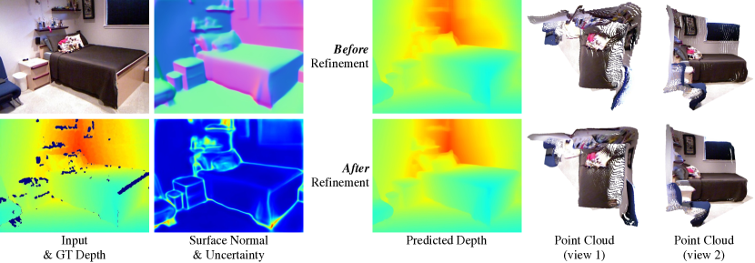
Figure 1: This figure shows how the proposed normal-guided depth refinement improves the quality of the 3D reconstruction. While the predicted depth-maps look similar, the point cloud comparison shows that the characteristics in the scene geometry (e.g., orientation of the walls) are better preserved in the refined output.

1 Introduction

Monocular 3D reconstruction is one of the fundamental problems in computer vision, with a wide variety of applications including autonomous driving [Geiger et al.(2012)Geiger, Lenz, and Urtasun], augmented reality [Huang et al.(2019)Huang, Zhou, Funkhouser, and Guibas], and 3D photography [Kopf et al.(2020)Kopf, Matzen, Alsisan, Quigley, Ge, Chong, Patterson, Frahm, Wu, Yu, et al.]. In this paper, we focus on two popular approaches in single image 3D reconstruction - surface normal estimation and depth estimation. The two problems are closely related as surface normal can also be computed from the predicted depth-map.

For both tasks, deep learning-based methods have shown impressive performance. However, if we calculate the surface normal from the output of depth estimation methods, its accuracy is significantly worse than that of surface normal estimation methods. For NYUv2 [Silberman et al.(2012)Silberman, Hoiem, Kohli, and Fergus] dataset, the surface normal calculated from the depth-map predicted by AdaBins [Bhat et al.(2021)Bhat, Alhashim, and Wonka] has mean angular error of $28.8^{\circ}$, which is nearly twice as large as $14.9^{\circ}$ achieved by the direct estimation of Bae et al. [Bae et al.(2021)Bae, Budvytis, and Cipolla]. This suggests that, while depth estimation methods show low per-pixel depth errors, the recovered surface does not faithfully capture the characteristics of the scene geometry (e.g., the walls and floors are not flat).

Poor surface normal accuracy of depth estimation methods is mainly caused by two problems. First is the imbalance in the training data. Fig. 2-(left) shows that most of the pixels in NYUv2 [Silberman et al.(2012)Silberman, Hoiem, Kohli, and Fergus] have ground truth depth of 1-4m. If depth estimation is solved as regression, the network is biased to predict those intermediate depth values, leading to poor surface normal accuracy. Secondly, estimating a depth-map with high surface normal accuracy requires view-dependent inference. Fig. 2-(right) shows that, for perspective camera, the depth-map corresponding to a flat surface is not linear. Unlike surface normal, the depth gradient is not constant within the surface and is dependent on the viewing direction. Depth estimation is thus difficult to solve using convolutional neural networks, which are designed to be translation-equivariant.

In this paper, we propose IronDepth, a novel framework that uses surface normal and its uncertainty to recurrently refine the initial depth-map (iron: iterative refinement of depth using normal). Given the estimated depth and surface normal of a pixel, we can define a plane. Then, for a query pixel, we can calculate how its depth should be updated in order for it to belong to the same plane. We call this the normal-guided depth propagation. We then formulate depth refinement as classification of choosing the neighboring pixel to propagate from. After refining the initial depth-map in a coarse resolution, we apply the same normal-guided depth propagation to sub-pixel points to upsample the refined output. Fig. 1 shows how the proposed normal-guided refinement improves the quality of the 3D reconstruction.

Our method achieves state-of-the-art performance on NYUv2 [Silberman et al.(2012)Silberman, Hoiem, Kohli, and Fergus]. We also outperform other methods in cross-dataset evaluation on iBims-1 [Koch et al.(2018)Koch, Liebel, Fraundorfer, and Korner]. While the improvement in depth accuracy is small, the surface normal calculated from our depth prediction is significantly more accurate than those obtained by the competing methods.

We also run additional experiments to further investigate the usefulness of the proposed surface normal-guided depth refinement module. Firstly, the initial depth prediction can be replaced with the output of the existing depth estimation methods to improve their accuracy. We confirmed this by applying our framework to five state-of-the-art depth estimation methods. Secondly, our framework can seamlessly be applied to depth completion. Given a sparse depth measurement, we can fix the depth for the pixels with measurement. This allows the information (i.e. sparse depth measurements) to be propagated to the neighboring pixels, improving the overall accuracy.

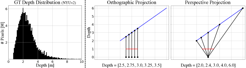
Figure 2: (left) This histogram shows the distribution of the ground truth depth in NYUv2 [Silberman et al.(2012)Silberman, Hoiem, Kohli, and Fergus] test set. Most of the pixels have depth of 1-4m, making the prediction biased to those intermediate values. (right) In this figure, the blue, red and black lines represent a flat surface, image plane and pixel rays, respectively. For orthographic projection, the depth values are linear within the image plane, and the gradient of depth is constant. For perspective projection, however, the depth gradient is dependent on the viewing direction, making the inference challenging for CNNs, which are designed to be translation-equivariant.

2 Related Work

Single image depth estimation. The goal of the problem is to estimate the per-pixel metric depth. Owing to the advances in deep neural networks (DNNs), state-of-the-art approaches [Eigen et al.(2014)Eigen, Puhrsch, and Fergus, Eigen and Fergus(2015b), Liu et al.(2015)Liu, Shen, and Lin, Laina et al.(2016)Laina, Rupprecht, Belagiannis, Tombari, and Navab, Cao et al.(2017)Cao, Wu, and Shen, Kuznietsov et al.(2017)Kuznietsov, Stuckler, and Leibe, Fu et al.(2018)Fu, Gong, Wang, Batmanghelich, and Tao, Lee et al.(2019)Lee, Han, Ko, and Suh, Yin et al.(2019)Yin, Liu, Shen, and Yan, Bhat et al.(2021)Bhat, Alhashim, and Wonka, Huynh et al.(2020)Huynh, Nguyen-Ha, Matas, Rahtu, and Heikkilä, Yang et al.(2021)Yang, Tang, Ding, Sebe, and Ricci] use DNNs to extract features and predict the per-pixel metric depth. While most methods solve depth estimation as regression, other methods recast the problem as classification [Cao et al.(2017)Cao, Wu, and Shen, Bhat et al.(2021)Bhat, Alhashim, and Wonka] or ordinal regression (i.e. classification on ordered thresholds) [Fu et al.(2018)Fu, Gong, Wang, Batmanghelich, and Tao] by discretizing the output depth. We propose a hybrid approach where the initial depth-map is obtained via regression and then refined by solving classification of selecting the neighboring pixel to propagate from.

Single image surface normal estimation. The goal of the problem is to estimate the per-pixel surface normal vector, defined in the camera-centered coordinates. Similar to depth estimation, this problem is solved via direct regression using DNNs [Wang et al.(2015)Wang, Fouhey, and Gupta, Eigen and Fergus(2015a), Bansal et al.(2016)Bansal, Russell, and Gupta, Liao et al.(2019)Liao, Gavves, and Snoek, Do et al.(2020)Do, Vuong, Roumeliotis, and Park, Bae et al.(2021)Bae, Budvytis, and Cipolla]. Notable contributions have been made by using a spatial rectifier to improve the performance on tilted images [Do et al.(2020)Do, Vuong, Roumeliotis, and Park], and using vision transformers [Carion et al.(2020)Carion, Massa, Synnaeve, Usunier, Kirillov, and Zagoruyko, Dosovitskiy et al.(2021)Dosovitskiy, Beyer, Kolesnikov, Weissenborn, Zhai, Unterthiner, Dehghani, Minderer, Heigold, Gelly, et al.] to encode the global context [Yang et al.(2021)Yang, Tang, Ding, Sebe, and Ricci]. While most methods only estimate the normal, recent work by Bae et al. [Bae et al.(2021)Bae, Budvytis, and Cipolla] also estimates the associated uncertainty. They also proposed to apply the training loss on a subset of pixels selected based on the estimated uncertainty, thereby improving the quality of prediction on small structures and near object boundaries.

Improving depth estimation using surface normal. Many attempts have been made to exploit the relationship between depth and surface normal. Yin et al. [Yin et al.(2019)Yin, Liu, Shen, and Yan] proposed virtual normal loss, where triplets of pixels are sampled during training and the surface normal of the triangle is computed from the predicted depth and the ground truth. They applied L1 loss between the computed normals. Long et al. [Long et al.(2021)Long, Lin, Liu, Li, Theobalt, Yang, and Wang] improved upon this work by adaptively combining the normals computed for different triplets. Our normal-guided depth propagation is inspired by GeoNet++ [Qi et al.(2020)Qi, Liu, Liao, Torr, Urtasun, and Jia], which iterates between depth-to-normal and normal-to-depth modules. The difference is three-fold. Firstly, the normal-to-depth module in [Qi et al.(2020)Qi, Liu, Liao, Torr, Urtasun, and Jia] is deterministic (i.e. no learnable parameter). The propagation weight between pixel $i$ and $j$ is determined by their surface normal similarity, $\mathbf{n}_{i}^{\intercal}\mathbf{n}_{j}$. This can fail if $i$ and $j$ belong to disconnected planes with similar surface normals. Instead, we learn the propagation weights in a recurrent framework. Secondly, we use surface normal uncertainty to avoid propagating from the pixels with high uncertainty. Lastly, we extend the normal-guided depth propagation to depth upsampling.

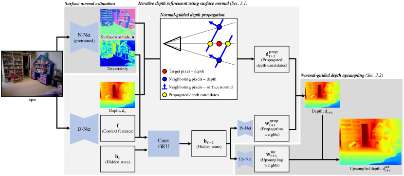
Figure 3: This figure illustrates the proposed IronDepth pipeline. Given the input image, N-Net estimates the pixel-wise surface normal and its uncertainty. D-Net estimates the initial low-resolution depth-map $d_{t=0}$. It also produces the context features f and hidden state $\textbf{h}_{t=0}$, which are passed through a ConvGRU [Cho et al.(2014)Cho, Van Merriënboer, Bahdanau, and Bengio] cell to produce $\textbf{h}_{t+1}$. With n and $d_{t}$, we can propagate the depth of the neighboring pixels to generate a set of depth candidates $\textbf{d}^{\text{prop}}_{t+1}$. The updated depth-map $d_{t+1}$ is then given as the weighted sum $\sum\textbf{d}^{\text{prop}}_{t+1}\textbf{w}^{\text{prop}}_{t+1}$, where $\textbf{w}^{\text{prop}}_{t+1}$ is estimated from $\textbf{h}_{t+1}$ using a lightweight CNN (Pr-Net). Lastly, we apply the same principle (normal-guided depth propagation $\rightarrow$ weighted sum) for sub-pixel points to obtain the full-resolution output.

3 Method

The proposed pipeline is illustrated in Fig. 3. It takes a single RGB image with known camera intrinsics as input. Firstly, we use an off-the-shelf network [Bae et al.(2021)Bae, Budvytis, and Cipolla] to estimate the pixel-wise surface normal and its uncertainty. Secondly, D-Net estimates an initial low-resolution depth-map, which is refined iteratively using the predicted surface normal as guidance (Sec. 3.1). Lastly, we propose normal-guided upsampling to recover the full resolution output (Sec. 3.2).

3.1 Iterative depth refinement using surface normal

While the predicted surface normal cannot give us the metric depth of a pixel, it tells us how the depth should change around each pixel. Our goal is to exploit such geometric constraint to improve the initial, unconstrained depth prediction. Firstly, we estimate an initial depth-map $d_{t=0}$ using a convolutional encoder-decoder (D-Net). Then, for each pixel, the depths of the neighboring pixels are propagated towards the central pixel, using the surface normal as guidance. The weighted sum of the propagated depths then gives us the updated depth-map $d_{t+1}$. To ensure computational efficiency, the refinement is performed in a coarse resolution.

Initial depth prediction. The initial depth-map, $d_{t=0}$, is estimated with D-Net, a lightweight convolutional encoder-decoder with EfficientNet B5 [Tan and Le(2019)] backbone. The architecture is same as the one used in [Bhat et al.(2021)Bhat, Alhashim, and Wonka], except that we only decode until $H/8\times W/8$ resolution, where $H$ and $W$ are the input height and width. Using the decoded feature-map as input, three sets of convolutional layers estimate (1) the initial depth-map $d_{t=0}$, (2) context feature f and (3) the initial hidden state $\textbf{h}_{t=0}$, all in $H/8\times W/8$ resolution.

Hidden state update. The hidden state $\mathbf{h}_{t}$ is updated recurrently using a Convolutional Gated Recurrent Unit [Cho et al.(2014)Cho, Van Merriënboer, Bahdanau, and Bengio] (ConvGRU). We use the architecture of [Teed and Deng(2020)]. The input to the ConvGRU cell is the concatenation of the context feature $\mathbf{f}$ and the surface normal confidence $\kappa$. Since higher value of $\kappa$ means that the predicted surface normal has lower uncertainty, the network can learn to propagate from the neighboring pixel with high $\kappa$.

Recurrent depth refinement. Consider a pixel $i$ with pixel coordinates $(u_{i},v_{i})$. Assuming a pinhole camera, its camera-centered coordinates $\mathbf{X}^{c}_{t}$ can be given as

$$\mathbf{X}^{c}_{t}(u_{i},v_{i})\!=\!\begin{bmatrix}\frac{u_{i}-u_{0}}{\alpha_{u}}\\ \frac{v_{i}-v_{0}}{\alpha_{v}}\\ 1\end{bmatrix}\cdot d_{t}(u_{i},v_{i})=\mathbf{r}(u_{i},v_{i})\cdot d_{t}(u_{i},v_{i})\;\;\text{,}\;\;\mathbf{K}=\begin{bmatrix}\alpha_{u}&0&u_{0}\\ 0&\alpha_{v}&v_{0}\\ 0&0&1\end{bmatrix},$$ (1)

where $\mathbf{r}(u_{i},v_{i})$ represents a ray with unit depth, $\mathbf{K}$ is the camera calibration matrix, and $t$ indexes the iteratively updated depth-map.

Now, consider a local neighborhood of pixel $i$, which can be defined as $\mathcal{N}_{i}=\{j\;:\;|u_{i}-u_{j}|\leq\beta\;\text{and}\;|v_{i}-v_{j}|\leq\beta\}$. We use $\beta=2$ in all experiments (i.e. $5\times 5$ neighborhood) as it led to a good balance between accuracy and computational efficiency. If the pixel $i$ belongs to the same plane as a neighboring pixel $j$ with depth $d_{t}(u_{j},v_{j})$ and surface normal $\mathbf{n}(u_{j},v_{j})$, its depth should be

$$d^{\text{prop}}_{t+1}(u_{i},v_{i},j)=\frac{\mathbf{n}^{\intercal}(u_{j},v_{j})\mathbf{r}(u_{j},v_{j})}{\mathbf{n}^{\intercal}(u_{j},v_{j})\mathbf{r}(u_{i},v_{i})}d_{t}(u_{j},v_{j}).$$ (2)

We call this the normal-guided depth propagation. In order for pixel $i$ to belong to the same plane as its neighboring pixel $j$, its depth should be updated to $d^{\text{prop}}_{t+1}(u_{i},v_{i},j)$. The values of $d^{\text{prop}}_{t+1}(u_{i},v_{i},j)$, computed for $j\in\mathcal{N}_{i}$, can be considered as the per-pixel candidates for the refined depth-map. The updated depth-map can thus be given as

$$d_{t+1}(u_{i},v_{i})=\sum_{j\in\mathcal{N}_{i}}w^{\text{prop}}_{t+1}(u_{i},v_{i},j)\cdot d^{\text{prop}}_{t+1}(u_{i},v_{i},j),$$ (3)

where $\mathbf{w}^{\text{prop}}_{t+1}(u_{i},v_{i})=\{w^{\text{prop}}_{t+1}(u_{i},v_{i},j)\}$ is estimated from the hidden state $\mathbf{h}_{t+1}$, using a light-weight CNN (see Appendix for the architecture). Eq. 3 shows that depth refinement can be formulated as a $K$-class classification, where $K$ is the number of pixels in the neighborhood $\mathcal{N}_{i}$. Note that the neighborhood $\mathcal{N}_{i}$ also includes the pixel $i$ itself, in which case $d^{\text{prop}}_{t+1}(u_{i},v_{i},i)=d_{t}(u_{i},v_{i})$. The network can thus choose not to update depth for certain pixels.

Normal-guided depth propagation (Eq. 2) is a view-dependent operation, which depends on the pixels coordinates $(u_{i},v_{i})$ and $(u_{j},v_{j})$. However, once the depth candidates $d^{\text{prop}}_{t+1}(u_{i},v_{i},j)$ are computed, choosing from them requires view-independent inference, making the problem easier for the network to learn.

3.2 Normal-guided depth upsampling

For computational efficiency, the depth-map is refined in a coarse resolution ($H/8\times W/8$). After refinement, the depth-map should be upsampled to match the input resolution. However, linearly upsampling the depth-map does not preserve the surface normal (see Fig. 2). To this end, we introduce normal-guided upsampling.

Normal-guided depth upsampling. For each pixel in high-resolution depth-map, we can propagate the depths of its $3\times 3$ neighbors in the coarse depth-map. Then, a lightweight CNN (i.e. Up-Net in Fig. 3) solves 9-class classification of choosing the coarse resolution neighbor to propagate from. The weighted sum of the propagated depth candidates gives us the upsampled depth-map $d^{\text{up}}_{t}$. We show in the experiments that using the proposed normal-guided upsampling leads to better surface normal accuracy than using bilinear upsampling.

Network training. The initial depth-map $d_{0}$, estimated by D-Net, is recurrently refined and upsampled for $N_{\text{iter}}$ times, producing $\{d^{\text{up}}_{t}\}$ where $t\in\{0,1,...,N_{\text{iter}}\}$. The loss is computed as a weighted sum of their L1 losses,

$$\mathcal{L}^{\text{depth}}=\sum_{i=0}^{N_{\text{iter}}}\gamma^{N_{\text{iter}}-i}||d^{\text{gt}}-d^{\text{up}}_{t}||_{1},$$ (4)

where $0<\gamma<1$ puts a bigger emphasis on the final output. Following [Teed and Deng(2020)], we set $\gamma=0.8$. $N_{\text{iter}}$ is set to 3 during training and 20 at test time.

4 Experimental Setup

Datasets. Our method is trained and tested on NYUv2 [Silberman et al.(2012)Silberman, Hoiem, Kohli, and Fergus], which consists of RGB-D frames covering 464 indoor scenes. After training, we also evaluate the network on iBims-1 [Koch et al.(2018)Koch, Liebel, Fraundorfer, and Korner] (contains 100 RGB-D frames) without fine-tuning to test its generalization ability. The ground truth surface normal for [Koch et al.(2018)Koch, Liebel, Fraundorfer, and Korner] is obtained by running PCA with $7\times 7$ neighborhood.

Evaluation protocol. We evaluate the refined depth-map both in terms of depth and normal. Depth accuracy is evaluated using the metrics defined in [Eigen et al.(2014)Eigen, Puhrsch, and Fergus]. We also compute surface normals from the predicted depth-map, by running per-pixel PCA with $7\times 7$ neighborhood. Then, the angular error between the computed surface normal and the ground truth is measured. Following [Fouhey et al.(2013)Fouhey, Gupta, and Hebert], we report the mean, median and root-mean-squared error (lower is better). We also report the percentage of pixels with error less than $[11.25^{\circ},22.5^{\circ},30^{\circ}]$ (higher is better).

Implementation details. The proposed pipeline is implemented with PyTorch [Paszke et al.(2019)Paszke, Gross, Massa, Lerer, Bradbury, Chanan, Killeen, Lin, Gimelshein, Antiga, et al.]. We use the AdamW optimizer [Loshchilov and Hutter(2019)] and schedule the learning rate using [Smith and Topin(2018)] with $lr_{\text{max}}=3.5\times 10^{-4}$. We train N-Net for 5 epochs with a batch size of 16. The other components are trained for 10 epochs with a batch size of 4. The EfficientNet [Tan and Le(2019)] backbone of D-Net is fixed with the weights from [Bhat et al.(2021)Bhat, Alhashim, and Wonka].

Method	Depth error			Depth accuracy			Normal error			Normal accuracy
	abs rel	rmse	$\log_{10}$	$\delta_{1}$	$\delta_{2}$	$\delta_{3}$	mean	median	rmse	$11.25^{\circ}$	$22.5^{\circ}$	$30^{\circ}$
GeoNet [Qi et al.(2018)Qi, Liao, Liu, Urtasun, and Jia]	0.142	0.499	0.062	0.801	0.963	0.992	41.5	35.5	50.2	11.7	30.5	42.2
DORN [Fu et al.(2018)Fu, Gong, Wang, Batmanghelich, and Tao]	0.106	0.397	0.046	0.877	0.970	0.990	44.7	39.3	53.3	9.2	26.7	38.0
VNL [Yin et al.(2019)Yin, Liu, Shen, and Yan]	0.100	0.368	0.043	0.895	0.980	0.996	26.8	17.0	37.9	36.3	59.4	68.6
BTS [Lee et al.(2019)Lee, Han, Ko, and Suh]	0.110	0.392	0.047	0.886	0.978	0.994	32.4	24.7	42.1	22.7	46.1	58.3
AdaBins [Bhat et al.(2021)Bhat, Alhashim, and Wonka]	0.103	0.364	0.044	0.902	0.983	0.997	28.8	20.7	38.6	28.3	53.2	64.7
TransDepth [Yang et al.(2021)Yang, Tang, Ding, Sebe, and Ricci]	0.106	0.365	0.045	0.900	0.983	0.996	30.0	22.4	39.7	25.6	50.2	62.4
Ours	0.101	0.352	0.043	0.910	0.985	0.997	20.8	11.3	31.9	49.7	70.5	77.9

Table 1: Quantitative evaluation on NYUv2 [Silberman et al.(2012)Silberman, Hoiem, Kohli, and Fergus]. We show state-of-the-art performance both in terms of depth and normal.

5 Experiments

In Sec. 5.1, we evaluate our method on NYUv2 [Silberman et al.(2012)Silberman, Hoiem, Kohli, and Fergus] and iBims-1 [Koch et al.(2018)Koch, Liebel, Fraundorfer, and Korner]. We make quantitative and qualitative comparison against the state-of-the-art methods and run ablation study experiments. In Sec. 5.2, we explore the usefulness of the proposed normal-guided depth propagation.

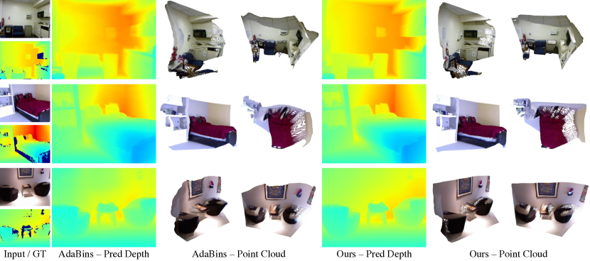
Figure 4: This figure provides a qualitative comparison between AdaBins [Bhat et al.(2021)Bhat, Alhashim, and Wonka] and our method. While the predicted depth-maps look similar, the point cloud comparison shows that our method is better at capturing the orientation of the surfaces.

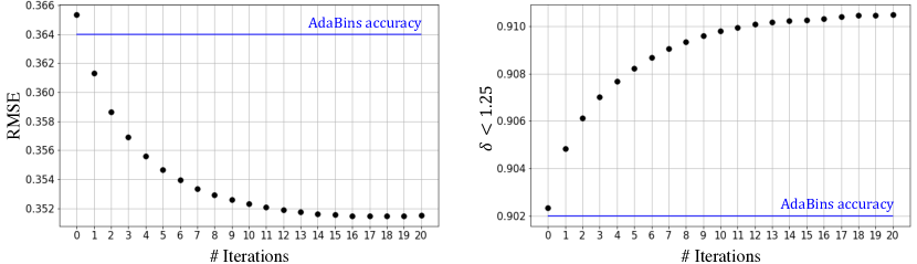
Figure 5: This figure shows how the accuracy on NYUv2 [Silberman et al.(2012)Silberman, Hoiem, Kohli, and Fergus] improves during the normal-guided iterative refinement. The accuracy converges after about 10 iterations.

Method	Depth error			Depth accuracy			Normal error			Normal accuracy			Planarity
	rel	rmse	$\log_{10}$	$\delta_{1}$	$\delta_{2}$	$\delta_{3}$	mean	median	rmse	$11.25^{\circ}$	$22.5^{\circ}$	$30^{\circ}$	$\epsilon^{\text{plan}}$	$\epsilon^{\text{orie}}$
SharpNet [Ramamonjisoa and Lepetit(2019)]	0.26	1.07	0.11	0.59	0.84	0.94	-	-	-	-	-	-	9.95	25.67
VNL [Yin et al.(2019)Yin, Liu, Shen, and Yan]	0.24	1.07	0.11	0.55	0.85	0.94	39.8	30.4	51.0	17.9	38.6	49.4	6.49	18.72
BTS [Lee et al.(2019)Lee, Han, Ko, and Suh]	0.24	1.08	0.12	0.53	0.84	0.94	44.0	37.8	53.5	13.0	29.5	40.0	7.25	20.52
DAV [Huynh et al.(2020)Huynh, Nguyen-Ha, Matas, Rahtu, and Heikkilä]	0.24	1.06	0.10	0.59	0.84	0.94	-	-	-	-	-	-	7.21	18.45
AdaBins [Bhat et al.(2021)Bhat, Alhashim, and Wonka]	0.22	1.06	0.11	0.55	0.86	0.95	37.1	29.6	46.9	18.0	38.7	50.6	6.25	17.51
Ours	0.21	1.03	0.11	0.59	0.87	0.95	25.3	14.2	37.4	43.1	63.9	71.6	3.29	8.48

Table 2: Cross-dataset evaluation on iBims-1 [Koch et al.(2018)Koch, Liebel, Fraundorfer, and Korner]. Our method shows significantly higher surface normal accuracy. We also outperform other methods in terms of planarity (quantifies how planar the prediction is for walls, table surfaces and floors).

5.1 Main results

NYUv2. Tab. 1 shows that our method achieves state-of-the-art performance on NYUv2 [Silberman et al.(2012)Silberman, Hoiem, Kohli, and Fergus]. While the differences in the depth metrics are small, the surface normals computed from our depth-maps are significantly more accurate than those obtained by the other methods. For example, the mean angular error ($20.8^{\circ}$) is 22.4% smaller than the second best method ($26.8^{\circ}$ achieved by [Yin et al.(2019)Yin, Liu, Shen, and Yan]). Fig. 4 provides a qualitative comparison against [Bhat et al.(2021)Bhat, Alhashim, and Wonka]. The point cloud comparison shows that our method faithfully captures the surface layout of the scene. Fig. 5 shows how the accuracy improves during the iterative refinement. Before refinement, the accuracy is similar to that of [Bhat et al.(2021)Bhat, Alhashim, and Wonka]. The accuracy improves quickly in the first few iterations and converges after about 10 iterations.

iBims-1. Tab. 2 evaluates the generalization ability on iBims-1 [Koch et al.(2018)Koch, Liebel, Fraundorfer, and Korner]. Similar to the results on NYUv2, we show a small improvement in depth accuracy, but a large improvement in surface normal accuracy. We also report $\epsilon^{\text{plan}}$ and $\epsilon^{\text{orie}}$ (defined in [Koch et al.(2018)Koch, Liebel, Fraundorfer, and Korner]), which quantify the planarity of the pixels belonging to walls, table surfaces and floors. We achieve 47.4% reduction in $\epsilon^{\text{plan}}$ and 51.6% reduction in $\epsilon^{\text{orie}}$, compared to AdaBins [Bhat et al.(2021)Bhat, Alhashim, and Wonka].

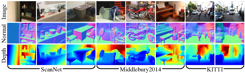
Figure 6: This figure shows predictions made by our method trained on NYUv2 [Silberman et al.(2012)Silberman, Hoiem, Kohli, and Fergus]. The network generalizes well to ScanNet [Dai et al.(2017)Dai, Chang, Savva, Halber, Funkhouser, and Nießner], Middlebury [Scharstein et al.(2014)Scharstein, Hirschmüller, Kitajima, Krathwohl, Nešić, Wang, and Westling] and KITTI [Geiger et al.(2012)Geiger, Lenz, and Urtasun].

Generalization. In Fig. 6, we further demonstrate the generalization ability of our method. As highlighted in [Bae et al.(2021)Bae, Budvytis, and Cipolla], surface normal estimation networks generalize well across different datasets as they rely on low-level cues (e.g., texture gradients, shading). Since IronDepth uses the predicted surface normal to refine the initial depth-map, it can generalize well even when the domain gap is large (e.g., train on indoor scenes $\rightarrow$ test on outdoor scenes).

Iterative	Upsample	Depth error			Depth accuracy			Normal error			Normal accuracy
Refinement	Method	abs rel	rmse	$\log_{10}$	$\delta_{1}$	$\delta_{2}$	$\delta_{3}$	mean	median	rmse	$11.25^{\circ}$	$22.5^{\circ}$	$30^{\circ}$
$\times$	Nearest	0.107	0.375	0.045	0.896	0.982	0.996	39.1	31.6	47.8	11.6	35.7	47.8
$\checkmark$		0.103	0.361	0.044	0.904	0.984	0.997	33.7	23.6	43.1	17.5	47.9	59.4
$\times$	Bilinear	0.106	0.370	0.045	0.898	0.983	0.996	31.4	22.9	41.6	25.1	49.3	60.9
$\checkmark$		0.103	0.356	0.044	0.906	0.985	0.997	22.7	12.2	34.6	47.6	67.6	75.0
$\times$	Normal	0.105	0.369	0.045	0.897	0.982	0.996	28.6	20.0	39.0	30.8	54.4	65.0
$\checkmark$	-guided	0.101	0.352	0.043	0.910	0.985	0.997	20.8	11.3	31.9	49.7	70.5	77.9

Table 3: Ablation study experiments. We train the pipeline with and without the iterative refinement, and also try different methods of depth upsampling.

Ablation study. Tab. 3 provides the results of the ablation study experiments. Iterative depth refinement with normal-guided depth propagation (Sec. 3.1) significantly improves the accuracy, both in terms of depth and normal. Compared to bilinear upsampling, the proposed normal-guided upsampling (Sec. 3.2) leads to better surface normal accuracy.

Inference speed. The inference time of the full pipeline is 66.26 ms, when measured on a single 2080Ti GPU. The proposed normal-guided depth refinement only takes 0.57ms per iteration. This is because the refinement is performed in a coarse resolution ($H/8\times W/8$).

5.2 Applications

Lastly, we discuss the possible applications of the proposed framework.

Method	Depth error			Depth accuracy			Normal error			Normal accuracy
	abs rel	rmse	$\log_{10}$	$\delta_{1}$	$\delta_{2}$	$\delta_{3}$	mean	median	rmse	$11.25^{\circ}$	$22.5^{\circ}$	$30^{\circ}$
DORN [Fu et al.(2018)Fu, Gong, Wang, Batmanghelich, and Tao]	0.106	0.397	0.046	0.877	0.970	0.990	44.7	39.3	53.3	9.2	26.7	38.0
DORN + Ours	0.099	0.359	0.042	0.898	0.978	0.993	21.3	11.8	32.5	48.5	69.6	77.1
VNL [Yin et al.(2019)Yin, Liu, Shen, and Yan]	0.100	0.368	0.043	0.895	0.980	0.996	26.8	17.0	37.9	36.3	59.4	68.6
VNL + Ours	0.097	0.353	0.042	0.902	0.983	0.996	20.5	11.0	31.7	50.6	71.0	78.2
BTS [Lee et al.(2019)Lee, Han, Ko, and Suh]	0.110	0.392	0.047	0.886	0.978	0.994	32.4	24.7	42.1	22.7	46.1	58.3
BTS + Ours	0.104	0.368	0.044	0.899	0.981	0.995	21.0	11.5	32.1	49.4	70.2	77.6
AdaBins [Bhat et al.(2021)Bhat, Alhashim, and Wonka]	0.103	0.364	0.044	0.902	0.983	0.997	28.8	20.7	38.6	28.3	53.2	64.7
AdaBins + Ours	0.100	0.351	0.042	0.911	0.985	0.997	20.7	11.3	31.8	49.9	70.6	78.0
TransDepth [Yang et al.(2021)Yang, Tang, Ding, Sebe, and Ricci]	0.106	0.365	0.045	0.900	0.983	0.996	30.0	22.4	39.7	25.6	50.2	62.4
TransDepth + Ours	0.103	0.352	0.043	0.906	0.984	0.997	20.6	11.1	31.7	50.3	70.9	78.3

Table 4: Normal-guided depth refinement applied to the existing depth estimation methods. The accuracy is improved across all metrics.

Application to existing depth estimation methods. The normal-guided depth refinement can be applied to the predictions made by the existing depth estimation methods. Specifically, we can replace the $d_{0}$ estimated by D-Net with the predictions made by other methods (the network is not fine-tuned for each method). Tab. 4 shows that the accuracy is improved across all metrics. Significant improvement in the surface normal accuracy suggests that our framework can be used as a post-processing tool to improve the surface normal accuracy of the existing monocular depth estimation methods. This also suggests that replacing our D-Net (i.e. lightweight convolutional encoder-decoder) with a more sophisticated architecture can further improve the accuracy.

# Measurements	Depth metrics (w/o scale-match)						Depth metrics (w/ scale-match)
	abs rel	rmse	$\log_{10}$	$\delta_{1}$	$\delta_{2}$	$\delta_{3}$	abs rel	rmse	$\log_{10}$	$\delta_{1}$	$\delta_{2}$	$\delta_{3}$
0	0.101	0.352	0.043	0.910	0.985	0.997	0.101	0.352	0.043	0.910	0.985	0.997
10	0.097	0.341	0.041	0.917	0.986	0.997	0.076	0.300	0.033	0.944	0.991	0.998
50	0.084	0.304	0.035	0.938	0.990	0.998	0.063	0.260	0.027	0.962	0.994	0.999
100	0.070	0.266	0.030	0.957	0.993	0.999	0.053	0.231	0.023	0.972	0.995	0.999
200	0.051	0.212	0.021	0.976	0.996	0.999	0.041	0.191	0.018	0.983	0.997	0.999

Table 5: We provide the ground truth for a small number of pixels and fix their values. The depths of those pixels are propagated to the neighboring pixels, improving the overall accuracy. We can also multiply the initial prediction by a factor that minimizes the error for the anchor points (before performing the refinement). Columns 8-13 show that applying such scale-matching leads to a bigger improvement.

Application to depth completion. Suppose that a network is trained to estimate depth from a single RGB image. If a new piece of information (e.g., sparse depth measurement from a LiDAR sensor) is available at test time, the network should be able to adapt to that information and the prediction should be more accurate. However, such ability to adapt is not possessed by most depth estimation methods. Since we refine the depth map by propagating information between the pixels, we can seamlessly apply our method to a scenario where sparse depth measurements are available (i.e. depth completion setup). Given a sparse depth measurement, we can add anchor points by fixing the depth for the pixels with measurement. We simulate this by providing the ground truth for a small number of pixels. Tab. 5 shows how the accuracy can be improved by adding such anchor points. The information provided for the anchor points (i.e. the measured depth) can be propagated to the neighboring pixels, making the overall prediction more accurate.

6 Conclusions

In this work, we proposed IronDepth, a novel framework that uses surface normal and its uncertainty to recurrently refine the predicted depth-map. We used normal-guided depth propagation to formulate depth refinement as classification of choosing the neighboring pixel to propagate from. Our method achieves state-of-the-art performance on NYUv2 [Silberman et al.(2012)Silberman, Hoiem, Kohli, and Fergus] and iBims-1 [Koch et al.(2018)Koch, Liebel, Fraundorfer, and Korner], both in terms of depth and surface normal. Point cloud comparison shows that our method is better at capturing the surface layout of the scene. The proposed framework can also be used as a post-processing tool for the existing depth estimation methods, or to propagate a sparse depth measurement to improve the overall accuracy.

Acknowledgement. This research was sponsored by Toshiba Europe’s Cambridge Research Laboratory.

Appendix A Network Architecture

Tab. 6 shows the architecture of D-Net, which estimates the initial depth-map $d_{t=0}$, context feature f and the initial hidden state $\mathbf{h}_{t=0}$. Tab. 7 shows the architecture of Pr-Net, which estimates the propagation weights $\mathbf{w}^{\text{prop}}_{t}$ for each iteration. Tab. 8 shows the architecture of Up-Net, which estimates the upsampling weights $\mathbf{w}^{\text{up}}_{t}$.

Input	Layer	Output	Output Dimension
image	-	-	$H\times W\times 3$
Encoder
image	EfficientNet B5	$F_{8}$	$H/8\times W/8\times 64$
		$F_{16}$	$H/16\times W/16\times 176$
		$F_{32}$	$H/32\times W/32\times 2048$
Decoder
$F_{32}$	Conv2D(ks=1, $C_{\text{out}}$=2048, padding=0)	$x_{0}$	$H/32\times W/32\times 2048$
$\text{up}(x_{0})+F_{16}$	$\left(\begin{matrix}\text{Conv2D(ks=3, $C_{\text{out}}$=1024, padding=1)},\\ \text{GroupNorm}(n_{\text{groups}}=8),\\ \text{LeakyReLU()}\end{matrix}\right)\times 2$	$x_{1}$	$H/16\times W/16\times 1024$
$\text{up}(x_{1})+F_{8}$	$\left(\begin{matrix}\text{Conv2D(ks=3, $C_{\text{out}}$=512, padding=1)},\\ \text{GroupNorm}(n_{\text{groups}}=8),\\ \text{LeakyReLU()}\end{matrix}\right)\times 2$	$x_{2}$	$H/8\times W/8\times 512$
Prediction Heads
$x_{2}$	Conv2D(ks=3, $C_{\text{out}}$=128, padding=1), ReLU(), Conv2D(ks=1, $C_{\text{out}}$=128, padding=0), ReLU(), Conv2D(ks=1, $C_{\text{out}}$=1, padding=0)	$d_{t=0}$	$H/8\times W/8\times 1$
$x_{2}$	Conv2D(ks=3, $C_{\text{out}}$=128, padding=1), ReLU(), Conv2D(ks=1, $C_{\text{out}}$=128, padding=0), ReLU(), Conv2D(ks=1, $C_{\text{out}}$=64, padding=0)	$\mathbf{f}$	$H/8\times W/8\times 64$
$x_{2}$	Conv2D(ks=3, $C_{\text{out}}$=128, padding=1), ReLU(), Conv2D(ks=1, $C_{\text{out}}$=128, padding=0), ReLU(), Conv2D(ks=1, $C_{\text{out}}$=64, padding=0)	$\mathbf{h}_{t=0}$	$H/8\times W/8\times 64$

Table 6: D-Net architecture. In each convolutional layer, "ks" means the kernel size and $C_{\text{out}}$ is the number of output channels. $F_{N}$ represents the feature-map of resolution $H/N\times W/N$. $X+Y$ means that the two tensors are concatenated, and $\text{up}(\cdot)$ is bilinear upsampling.

Input	Layer	Output	Output Dimension
$\mathbf{h}_{t}$	Conv2D(ks=3, $C_{\text{out}}=128$, padding=1), ReLU(), Conv2D(ks=1, $C_{\text{out}}=128$, padding=0), ReLU(), Conv2D(ks=1, $C_{\text{out}}=5\times 5$, padding=0)	$\mathbf{w}^{\text{prop}}_{t}$	$H/8\times W/8\times(5\times 5)$

Table 7: Architecture of Pr-Net. Pr-Net estimates the propagation weights $\mathbf{w}^{\text{prop}}_{t}$.

Input	Layer	Output	Output Dimension
$\mathbf{h}_{t}$	Conv2D(ks=3, $C_{\text{out}}$=128, padding=1), ReLU(), Conv2D(ks=1, $C_{\text{out}}$=128, padding=0), ReLU(), Conv2D(ks=1, $C_{\text{out}}$=$8\times 8\times 9$, padding=0)	$\mathbf{w}^{\text{up}}_{t}$	$H/8\times W/8\times(8\times 8\times 9)$

Table 8: Architecture of Up-Net. Up-Net estimates the upsampling weights $\mathbf{w}^{\text{up}}_{t}$.

References

- [Bae et al.(2021)Bae, Budvytis, and Cipolla] Gwangbin Bae, Ignas Budvytis, and Roberto Cipolla. Estimating and exploiting the aleatoric uncertainty in surface normal estimation. In Proc. of IEEE/CVF International Conference on Computer Vision (ICCV), 2021.
- [Bansal et al.(2016)Bansal, Russell, and Gupta] Aayush Bansal, Bryan Russell, and Abhinav Gupta. Marr revisited: 2d-3d alignment via surface normal prediction. In Proc. of IEEE/CVF Conference on Computer Vision and Pattern Recognition (CVPR), 2016.
- [Bhat et al.(2021)Bhat, Alhashim, and Wonka] Shariq Farooq Bhat, Ibraheem Alhashim, and Peter Wonka. Adabins: Depth estimation using adaptive bins. In Proc. of IEEE/CVF Conference on Computer Vision and Pattern Recognition (CVPR), 2021.
- [Cao et al.(2017)Cao, Wu, and Shen] Yuanzhouhan Cao, Zifeng Wu, and Chunhua Shen. Estimating depth from monocular images as classification using deep fully convolutional residual networks. IEEE Transactions on Circuits and Systems for Video Technology, 28(11):3174–3182, 2017.
- [Carion et al.(2020)Carion, Massa, Synnaeve, Usunier, Kirillov, and Zagoruyko] Nicolas Carion, Francisco Massa, Gabriel Synnaeve, Nicolas Usunier, Alexander Kirillov, and Sergey Zagoruyko. End-to-end object detection with transformers. In Proc. of European Conference on Computer Vision (ECCV), 2020.
- [Cho et al.(2014)Cho, Van Merriënboer, Bahdanau, and Bengio] Kyunghyun Cho, Bart Van Merriënboer, Dzmitry Bahdanau, and Yoshua Bengio. On the properties of neural machine translation: Encoder-decoder approaches. In Eighth Workshop on Syntax, Semantics and Structure in Statistical Translation (SSST-8), 2014.
- [Dai et al.(2017)Dai, Chang, Savva, Halber, Funkhouser, and Nießner] Angela Dai, Angel X Chang, Manolis Savva, Maciej Halber, Thomas Funkhouser, and Matthias Nießner. Scannet: Richly-annotated 3d reconstructions of indoor scenes. In Proc. of IEEE/CVF Conference on Computer Vision and Pattern Recognition (CVPR), 2017.
- [Do et al.(2020)Do, Vuong, Roumeliotis, and Park] Tien Do, Khiem Vuong, Stergios I Roumeliotis, and Hyun Soo Park. Surface normal estimation of tilted images via spatial rectifier. In Proc. of European Conference on Computer Vision (ECCV), 2020.
- [Dosovitskiy et al.(2021)Dosovitskiy, Beyer, Kolesnikov, Weissenborn, Zhai, Unterthiner, Dehghani, Minderer, Heigold, Gelly, et al.] Alexey Dosovitskiy, Lucas Beyer, Alexander Kolesnikov, Dirk Weissenborn, Xiaohua Zhai, Thomas Unterthiner, Mostafa Dehghani, Matthias Minderer, Georg Heigold, Sylvain Gelly, et al. An image is worth 16x16 words: Transformers for image recognition at scale. In International Conference on Learning Representations (ICLR), 2021.
- [Eigen and Fergus(2015a)] David Eigen and Rob Fergus. Predicting depth, surface normals and semantic labels with a common multi-scale convolutional architecture. In Proc. of IEEE/CVF International Conference on Computer Vision (ICCV), 2015a.
- [Eigen and Fergus(2015b)] David Eigen and Rob Fergus. Predicting depth, surface normals and semantic labels with a common multi-scale convolutional architecture. In Proc. of IEEE/CVF International Conference on Computer Vision (ICCV), 2015b.
- [Eigen et al.(2014)Eigen, Puhrsch, and Fergus] David Eigen, Christian Puhrsch, and Rob Fergus. Depth map prediction from a single image using a multi-scale deep network. In Proc. of Advances in Neural Information Processing Systems (NeurIPS), 2014.
- [Fouhey et al.(2013)Fouhey, Gupta, and Hebert] David F Fouhey, Abhinav Gupta, and Martial Hebert. Data-driven 3d primitives for single image understanding. In Proc. of IEEE/CVF International Conference on Computer Vision (ICCV), 2013.
- [Fu et al.(2018)Fu, Gong, Wang, Batmanghelich, and Tao] Huan Fu, Mingming Gong, Chaohui Wang, Kayhan Batmanghelich, and Dacheng Tao. Deep ordinal regression network for monocular depth estimation. In Proc. of IEEE/CVF Conference on Computer Vision and Pattern Recognition (CVPR), 2018.
- [Geiger et al.(2012)Geiger, Lenz, and Urtasun] Andreas Geiger, Philip Lenz, and Raquel Urtasun. Are we ready for autonomous driving? the kitti vision benchmark suite. In Proc. of IEEE/CVF Conference on Computer Vision and Pattern Recognition (CVPR), 2012.
- [Huang et al.(2019)Huang, Zhou, Funkhouser, and Guibas] Jingwei Huang, Yichao Zhou, Thomas Funkhouser, and Leonidas J Guibas. Framenet: Learning local canonical frames of 3d surfaces from a single rgb image. In Proc. of IEEE/CVF International Conference on Computer Vision (ICCV), 2019.
- [Huynh et al.(2020)Huynh, Nguyen-Ha, Matas, Rahtu, and Heikkilä] Lam Huynh, Phong Nguyen-Ha, Jiri Matas, Esa Rahtu, and Janne Heikkilä. Guiding monocular depth estimation using depth-attention volume. In Proc. of European Conference on Computer Vision (ECCV), 2020.
- [Koch et al.(2018)Koch, Liebel, Fraundorfer, and Korner] Tobias Koch, Lukas Liebel, Friedrich Fraundorfer, and Marco Korner. Evaluation of cnn-based single-image depth estimation methods. In Proc. of European Conference on Computer Vision Workshops, 2018.
- [Kopf et al.(2020)Kopf, Matzen, Alsisan, Quigley, Ge, Chong, Patterson, Frahm, Wu, Yu, et al.] Johannes Kopf, Kevin Matzen, Suhib Alsisan, Ocean Quigley, Francis Ge, Yangming Chong, Josh Patterson, Jan-Michael Frahm, Shu Wu, Matthew Yu, et al. One shot 3d photography. ACM Transactions on Graphics (TOG), 39(4):76–1, 2020.
- [Kuznietsov et al.(2017)Kuznietsov, Stuckler, and Leibe] Yevhen Kuznietsov, Jorg Stuckler, and Bastian Leibe. Semi-supervised deep learning for monocular depth map prediction. In Proc. of IEEE/CVF Conference on Computer Vision and Pattern Recognition (CVPR), 2017.
- [Laina et al.(2016)Laina, Rupprecht, Belagiannis, Tombari, and Navab] Iro Laina, Christian Rupprecht, Vasileios Belagiannis, Federico Tombari, and Nassir Navab. Deeper depth prediction with fully convolutional residual networks. In International Conference on 3D Vision (3DV), 2016.
- [Lee et al.(2019)Lee, Han, Ko, and Suh] Jin Han Lee, Myung-Kyu Han, Dong Wook Ko, and Il Hong Suh. From big to small: Multi-scale local planar guidance for monocular depth estimation. arXiv preprint arXiv:1907.10326, 2019.
- [Liao et al.(2019)Liao, Gavves, and Snoek] Shuai Liao, Efstratios Gavves, and Cees GM Snoek. Spherical regression: Learning viewpoints, surface normals and 3d rotations on n-spheres. In Proc. of IEEE/CVF Conference on Computer Vision and Pattern Recognition (CVPR), 2019.
- [Liu et al.(2015)Liu, Shen, and Lin] Fayao Liu, Chunhua Shen, and Guosheng Lin. Deep convolutional neural fields for depth estimation from a single image. In Proc. of IEEE/CVF Conference on Computer Vision and Pattern Recognition (CVPR), 2015.
- [Long et al.(2021)Long, Lin, Liu, Li, Theobalt, Yang, and Wang] Xiaoxiao Long, Cheng Lin, Lingjie Liu, Wei Li, Christian Theobalt, Ruigang Yang, and Wenping Wang. Adaptive surface normal constraint for depth estimation. In Proc. of IEEE/CVF International Conference on Computer Vision (ICCV), 2021.
- [Loshchilov and Hutter(2019)] Ilya Loshchilov and Frank Hutter. Decoupled weight decay regularization. International Conference on Learning Representations (ICLR), 2019.
- [Paszke et al.(2019)Paszke, Gross, Massa, Lerer, Bradbury, Chanan, Killeen, Lin, Gimelshein, Antiga, et al.] Adam Paszke, Sam Gross, Francisco Massa, Adam Lerer, James Bradbury, Gregory Chanan, Trevor Killeen, Zeming Lin, Natalia Gimelshein, Luca Antiga, et al. Pytorch: An imperative style, high-performance deep learning library. In Proc. of Advances in Neural Information Processing Systems (NeurIPS), 2019.
- [Qi et al.(2018)Qi, Liao, Liu, Urtasun, and Jia] Xiaojuan Qi, Renjie Liao, Zhengzhe Liu, Raquel Urtasun, and Jiaya Jia. Geonet: Geometric neural network for joint depth and surface normal estimation. In Proc. of IEEE/CVF Conference on Computer Vision and Pattern Recognition (CVPR), 2018.
- [Qi et al.(2020)Qi, Liu, Liao, Torr, Urtasun, and Jia] Xiaojuan Qi, Zhengzhe Liu, Renjie Liao, Philip HS Torr, Raquel Urtasun, and Jiaya Jia. Geonet++: Iterative geometric neural network with edge-aware refinement for joint depth and surface normal estimation. IEEE Transactions on Pattern Analysis and Machine Intelligence (TPAMI), 2020.
- [Ramamonjisoa and Lepetit(2019)] Michael Ramamonjisoa and Vincent Lepetit. Sharpnet: Fast and accurate recovery of occluding contours in monocular depth estimation. In Proc. of IEEE/CVF International Conference on Computer Vision Workshops, 2019.
- [Scharstein et al.(2014)Scharstein, Hirschmüller, Kitajima, Krathwohl, Nešić, Wang, and Westling] Daniel Scharstein, Heiko Hirschmüller, York Kitajima, Greg Krathwohl, Nera Nešić, Xi Wang, and Porter Westling. High-resolution stereo datasets with subpixel-accurate ground truth. In German Conference on Pattern Recognition (GCPR), 2014.
- [Silberman et al.(2012)Silberman, Hoiem, Kohli, and Fergus] Nathan Silberman, Derek Hoiem, Pushmeet Kohli, and Rob Fergus. Indoor segmentation and support inference from rgbd images. In Proc. of European Conference on Computer Vision (ECCV), 2012.
- [Smith and Topin(2018)] Leslie N Smith and Nicholay Topin. Super-convergence: Very fast training of residual networks using large learning rates. arXiv preprint arXiv:1708.07120, 2018.
- [Tan and Le(2019)] Mingxing Tan and Quoc Le. Efficientnet: Rethinking model scaling for convolutional neural networks. In International Conference on Machine Learning (ICML), 2019.
- [Teed and Deng(2020)] Zachary Teed and Jia Deng. Raft: Recurrent all-pairs field transforms for optical flow. In Proc. of European Conference on Computer Vision (ECCV), 2020.
- [Wang et al.(2015)Wang, Fouhey, and Gupta] Xiaolong Wang, David Fouhey, and Abhinav Gupta. Designing deep networks for surface normal estimation. In Proc. of IEEE/CVF Conference on Computer Vision and Pattern Recognition (CVPR), 2015.
- [Yang et al.(2021)Yang, Tang, Ding, Sebe, and Ricci] Guanglei Yang, Hao Tang, Mingli Ding, Nicu Sebe, and Elisa Ricci. Transformers solve the limited receptive field for monocular depth prediction. In Proc. of IEEE/CVF International Conference on Computer Vision (ICCV), 2021.
- [Yin et al.(2019)Yin, Liu, Shen, and Yan] Wei Yin, Yifan Liu, Chunhua Shen, and Youliang Yan. Enforcing geometric constraints of virtual normal for depth prediction. In Proc. of IEEE/CVF International Conference on Computer Vision (ICCV), 2019.