A Closer Look at Hardware-Friendly
Weight Quantization

Abstract

Quantizing a Deep Neural Network (DNN) model to be used on a custom accelerator with efficient fixed-point hardware implementations, requires satisfying many stringent hardware-friendly quantization constraints to train the model. We evaluate the two main classes of hardware-friendly quantization methods in the context of weight quantization: the traditional Mean Squared Quantization Error (MSQE)-based methods and the more recent gradient-based methods. We study the two methods on MobileNetV1 and MobileNetV2 using multiple empirical metrics to identify the sources of performance differences between the two classes, namely, sensitivity to outliers and convergence instability of the quantizer scaling factor. Using those insights, we propose various techniques to improve the performance of both quantization methods - they fix the optimization instability issues present in the MSQE-based methods during quantization of MobileNet models and allow us to improve validation performance of the gradient-based methods by 4.0% and 3.3% for MobileNetV1 and MobileNetV2 on ImageNet respectively.

1 Introduction

Recently there has been a rapid increase in demand for deploying Deep Neural Network (DNN)-based inference tasks on battery-powered edge devices for privacy and latency requirements. A hardware-based DNN accelerator designed for an specific application is shown to be a promising approach to process such computationally challenging tasks under a tight power budget constraint, which is much faster and significantly power-efficient than a general purpose DNN accelerator [27]. In order to compress a DNN model small enough to fit it onto such an accelerator, quantization methods need to deal with more stringent constraints [9] such as uniform and symmetric quantization, power-of-2 (PO2) scaling factors, and batch normalization layer folding [13]. The goal is to quantize model weights down to 4 bits or lower, but even with quantization-aware training, doing so without incurring a significant accuracy loss remains a challenging research problem for the community.

There are two main classes of quantizer optimization methods for quantization aware training: the Mean Squared Quantization Error (MSQE)-based methods [1, 7, 24, 29, 11] and the more recent gradient-based methods [15, 16, 28, 5, 8, 23]. The MSQE-based methods iteratively search for optimal quantizer parameters at each training step minimizing the MSQE between the full-precision value and its quantized low-precision counterpart. There are also MSQE-based methods which formulate the optimization problem to directly minimize the loss as in [11, 10]. QKeras [7], a popular framework for hardware-friendly quantization aware-training, has extended the MSQE-based methods with the hardware-friendly constraints. The gradient-based methods optimize the quantization parameters directly during gradient descent steps, so they can be jointly learned with other network parameters to minimize the loss function.  [5] developed a method to learn a clipping parameter for activation function.  [8] proposed a learnable scaling factor and means to estimate and scale their gradients to jointly train with other network parameters.  [15] suggested a gradient-based hardware-friendly quantizer which optimizes power-of-2 (PO2) constrained clipping range.

In this paper we study MSQE- and gradient-based methods for weight quantization on commonly used vision backbones with the objective of understanding the sources (underlying causes) of performance difference between the two classes of method. Based on our insights, we propose improvements to the training process that increase stability of training and the performance of the final models to achieve validation accuracy of $66.9\pm 0.17\%$ on MobileNetV1 and $67.5\pm 0.01\%$ on MobileNetV2. To the best of our knowledge, we are not aware of any work in the literature that satisfies all our hardware-friendliness constraints. The code for the quantizers will be available on Github .

The rest of the paper is organized as follows. Section 2 provides background on hardware-friendly quantization and describes the two main classes of hardware-friendly quantizers. In Section 3, we analyze the effects of quantization during training of the quantizers, and we improve the performance of both quantizers based on the findings of the analysis. Finally, experiments and conclusion can be found in Section 4 and Section 5, respectively.

2 Background

In this section, we describe hardware-friendly quantization constraints for efficient custom hardware implementation and the two main classes of hardware-friendly quantization methods used in our study.

2.1 Quantization for Deep Neural Networks

Quantization in DNN is a process of carefully searching for quantization parameters such as the scaling factor ($\Delta$) in (1) below to map model parameters (e.g., weight, bias) and/or activations from a large set to approximated values in a finite and smaller set using a function $Q:\mathbb{R}\rightarrow C$ with minimum accuracy degradation as shown in (1).

$$w_{q}=Q(w,\Delta)=\Delta\cdot\operatorname{clip}(\operatorname{round}(\frac{w}{\Delta});q_{\min},q_{\max}),\;\text{where}\;w\in R,w_{q}\in C$$ (1)

2.2 Hardware-Friendly Quantizer Constraints

Uniform quantization, which has uniformly spaced quantization levels, is often preferred due to its simplicity in hardware. Non-uniform quantization techniques like K-mean clustering based methods requires code-book look-up table related hardware overhead and logarithmic based methods can have a problem so called rigid resolution [20]. Adding multiple logarithmic quantization terms was suggested to solve the problem [20], however it incurs hardware overhead.

Symmetric quantization has a symmetrical number of quantization levels around zero. It has less hardware overhead than asymmetric quantization as the zero point (i.e., quantization range offset) is 0. Even some terms related to the zero point (when it is non-zero) can be pre-computed and added to the bias, however there is a term unavoidably calculated on-the-fly with respect to the input [18].

Per-tensor (layer) quantization has a single scaling factor (and zero point) per entire tensor. It has better hardware efficiency than per-channel quantization, which has different scaling factor for each output channel of the tensor, since all the accumulators for entire tensor operate using the same scaling factor.

Batch Normalization (BN) layer folding [18] reduces the two-step computations of the batch-normalized convolution to a one-step convolution by merging batch normalization operation with the weight and the bias of an adjacent linear layer [13].

Power-of-2 (PO2) scaling factor improves the hardware efficiency by constraining the scaling factor to a power-of-2 integer (that is to $2^{s}$ where $s$ is an integer) as then the scaling operation only requires a simple bit-shift operation instead of a fixed point multiplication. However, it often results in the accuracy degradation since the expressiveness of the scaling factor is limited.

2.3 MSQE-based Hardware-Friendly Quantizer

An MSQE-based hardware-friendly quantizer directly optimizes the PO2 scaling factor to minimize the mean squared quantization error [7], in its basic form, which is shown in (2).

$${\Delta_{\operatorname{PO2}}^{*}=\operatorname*{arg\,min}_{\Delta_{PO2}}||Q(w,\Delta_{PO2})-w||^{2}}\;,\;\textrm{where}\;\Delta_{PO2}=PO2(\Delta)=2^{\operatorname{round}(\log_{2}(\Delta))}$$ (2)

Algorithm 1 describes a pseudo-code of the MSQE optimization. It reduce the quantization problem to a linear regression problem with a closed form solution to find an optimal scaling factor in terms of the minimum MSQE, where it iteratively performs least squares fits at each training step [29]. The initial scaling factor $\Delta_{init}$ can be either the previously found scaling factor or a rough estimation based on the input distribution. We call it $\sf{MSQE}$ and use it as the baseline (and specifically the implementation from QKeras [2] (i.e., quantized_bits)) for the MSQE-based hardware-friendly quantizer in our study.

Algorithm 1 MSQE-based Optimization

$w,{\Delta_{init}},{N}_{iters}$

${\Delta_{PO2}}$

procedure :

     $q\leftarrow\frac{Q(w,\Delta_{init})}{\Delta_{init}}$

     $N\leftarrow{N}_{iters}$

     while $N\neq 0$ do

         $\Delta\leftarrow\cfrac{q^{T}w}{q^{T}q}$ $\triangleright$ Find an unconstrained optimal $\Delta$ minimizing the MSQE.

         $\Delta_{PO2}\leftarrow PO2(\Delta)$ $\triangleright$ Constrain $\Delta$ to be a power-of-2 value.

         $q\leftarrow\frac{Q(w,\Delta_{PO2})}{\Delta_{PO2}}$ $\triangleright$ Quantize w with the newly found $\Delta_{PO2}$.

         $N\leftarrow N-1$

     end while

end procedure

2.4 Gradient-based Hardware-Friendly Quantizer

A gradient-based hardware-friendly quantizer learns the PO2 scaling factor from the gradients seeking to optimize the scaling factor to minimize the task loss directly instead of locally optimizing the MSQE objective at each training iteration [8, 15, 4]. However, training $\Delta$ (in (2)) from the gradients can cause a numerical problem as the input to the $\log_{2}$ function can become negative by gradient update. It can be resolved by learning the scaling factor directly in the log domain ($\Delta_{\log_{2}}$) without $\log_{2}$ function [15] as shown in (3).

$$\Delta_{PO2}=PO2(\Delta_{\log_{2}})=2^{{\rm round}(\Delta_{\log_{2}})}$$ (3)

The local gradient of $\Delta_{\log_{2}}$ has dependency with the magnitude of the scaling factor ($2^{\Delta_{\log_{2}}}$) (see (4)), which can cause training instability (too large gradient) or slow convergence (too small gradient) depending on the scaling factor value [15]. To lessen the problem,  [15] suggests a method to normalize the gradient with its moving average variance and clip any large gradients for SGD training. However, it also reports that using Adam [17] optimizer without the normalization works well.

$$\begin{split}\frac{\partial w_{q}}{\partial\Delta_{\log_{2}}}=\frac{\partial w_{q}}{\partial\Delta_{PO2}}\cdot\frac{\partial\Delta_{PO2}}{\partial\Delta_{\log_{2}}}:=\frac{\partial w_{q}}{\partial\Delta_{PO2}}\cdot 2^{\Delta_{\log_{2}}}\cdot\ln 2\end{split}$$ (4)

The scaling factor can be initialized in several ways based on input values. It can be based on the dynamic range of the inputs, the input distributions [8, 15], and MSQE-optimal scaling factor [4]. We use a quantizer based on [15] as the baseline for the gradient-based hardware-friendly quantizer, and call it $\sf{GRAD}$.

3 Improving the Hardware-Friendly Quantizers

We analyze the advantages and disadvantages of both quantizer types and improve their performance based on our analysis.

3.1 Improving $\sf{MSQE}$

3.1.1 Sub-optimality in the Optimization of $\sf{MSQE}$

Algorithm 1 can converge to a sub-optimal solution as it makes a linear approximation to the original discrete non-linear problem. The sub-optimality can be improved by using a line search algorithm, where it simply searches for an MSQE-optimal PO2 scaling factor from the vicinity of the solution from Algorithm 1 (we will call the method as $\sf{finetune}$ in this paper.) (See Appendix A for an example and the method in detail.).

3.1.2 A Problem with Outliers in $\sf{MSQE}$

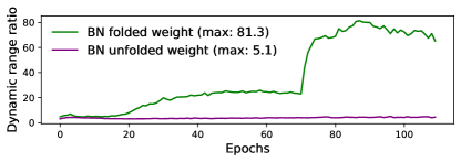
Figure 12: It shows that the ratios between the maximum and the minimum dynamic range (within the channels of a layer) for the BN (Batch Normalization) folded weight and the BN unfolded weight, which were averaged across all the layers, from training MobileNetV1 with $\it{MSQE}(finetune)$ quantizers. We can see that the BN folded weight generally had higher ratios compared to the BN unfolded one during training (about 15.9 times higher maximum dynamic range ratio).

A quantizer should make good trade-off between rounding and clipping errors in order to keep the precision of the majority of the input values in the presence of outliers. However, Algorithm 1 quantizes the input values uniformly between the largest and smallest values, so it is highly sensitive to outliers due to the squared error term in the optimization objective. This can be problematic especially for per-tensor quantization with batch normalization (BN) folding, where difference in the dynamic range of the weights between the channels can be large (see Figure 12 in the Appendix for details.). Figure 1 shows that the $\sf{MSQE}(baseline)$ and $\sf{MSQE}(finetune)$ were unstable and diverged, when $\sf{GRAD}$ was stable, during training quantized MobileNetV1 on ImageNet from scratch. The various metrics of a layer in Figure 1 shows that the scaling factor of $\sf{MSQE}(finetune)$ followed the rapidly increasing dynamic ranges of the input (weight) values causing about 80$\%$ of them to round to zero, which leaded to training divergence. On the other hand, $\sf{GRAD}$ had a well-controlled scaling factor in comparison.

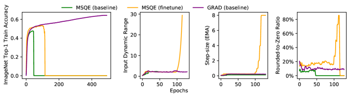
Figure 1: $\sf{MSQE}$ and $\sf{MSQE}(finetune)$ were unstable and diverged due to outliers, while $\sf{GRAD}$ was stable, during training quantized MobileNetV1 (4W4A) from scratch on ImageNet.

To reduce the sensitivity to outliers, a weighting factor can be used to suppress them during the MSQE optimization at each training step by performing a weighted least squares fit for Algorithm 1 and a weighted line search (see the Appendix B for the method in detail.).  (5) shows a simple outlier mask ($M_{outlier}$) using a percentile based threshold ($\sigma_{outlier}$) (assuming the input ($w$) has a Gaussian distribution) to suppress outliers, where each element in the outlier mask gets either 1 or 0 depending on whether its corresponding (absolute) input value is less than the threshold or not.

$$M_{outlier}=\begin{cases}0&\text{if }|w|\geq\sigma_{outlier}\cdot\sigma(w)\\ 1&\text{if }|w|<\sigma_{outlier}\cdot\sigma(w)\end{cases}$$ (5)

Figure 2 shows experiments using the outlier masking method with various standard deviations as the threshold. As we can see, the method didn’t solve the problem entirely, however it is clear that the training stability improved over the one without the method ($\sigma_{outlier}$ $\infty$).

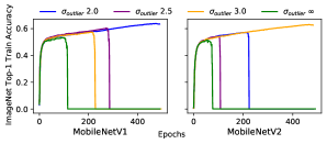
Figure 2: The outlier method with the threshold of various standard deviations ($\sigma_{outlier}$ 2.0, 2.5, and 3.0) improves training stability compared to the one without the method ($\sigma_{outlier}$ $\infty$), but it does not solve the outlier problem entirely.

3.1.3 Gradient Variance Awareness (GVA) Heuristic for Loss-Aware Optimization of $\sf{MSQE}$

Algorithm  1 optimizes uniformly across all the input values without considering their $\it{importance}$ in the loss function. Similarly to [6, 10, 11], it can be improved by formulating the optimization objective as minimizing the second-order approximated loss degradation from quantization, which is often further simplified by ignoring the first-order term assuming the loss is near a local minimum, which is shown in (6).

$$\operatorname*{arg\,min}_{\Delta_{po2}}\mathbb{E}[L(w_{q})-L(w)] \approx\mathbb{E}[\frac{\partial L(w)}{\partial w}^{T}(w_{q}-w)+\frac{1}{2}(w_{q}-w)^{T}H(w)(w_{q}-w)]$$ (6)

$$\approx\mathbb{E}[\frac{1}{2}(w_{q}-w)^{T}H(w)(w_{q}-w)]$$

$$where, \;w_{q}=Q(w,\Delta_{po2}),\;H(w)=\frac{\partial^{2}L(w)}{\partial w^{2}}$$

In practice, the Hessian in (6) is approximated by a diagonal matrix [30], which is sometimes further approximated by the (diagonal) empirical Fisher due to computational challenges for accurately estimating the diagonal entries of the Hessian [6]. However, even the empirical Fisher approximation practically works well in some cases, conditions and assumptions that make the approximation valid are unlikely to be satisfied in practice [19]. For computational efficiency, the optimization problem solved in our study (see (7)), we use the (diagonal) empirical Fisher approximation ($v_{j}$ is a running average of the second (raw) order moments of the j-th weight element ($w_{j}$) of a layer) as a gradient variance metric to minimize the quantization error for more dynamically changing weights during training, which is similar to the gradient noise adaptation perspective in [19] (we call the method as gradient variance aware (GVA) optimization in our study.).

$$\operatorname*{arg\,min}_{\Delta_{PO2}} \;\frac{1}{2}\sum_{j=1}^{N_{w}}v_{j}\cdot(Q(w_{j},\Delta_{PO2})-w_{j})^{2}$$ (7)

The method provides an additional benefit of suppressing outliers during training, which can complement the outlier method, since the running-averaged second (raw) order moments of the clipped inputs gradually decrease as long as they are clipped. Figure 3 (left) shows that the average second (raw) order moment ratio between the outliers and the inliers of weight (averaged across all the layers) for training quantized MobileNetV1 and MobileNetV2 with $\sf{MSQE}$ with $\sf{finetune}$ and GVA ($\sf{MSQE}(finetune,GVA)$). The ratios become smaller as the models are trained longer which means that outlier weights tend to be de-emphasized for the MSQE optimization when the GVA method is used. Figure 3 (right) also shows the effectiveness of the GVA method that the models were able to be trained from scratch without the outlier mask method.

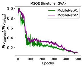
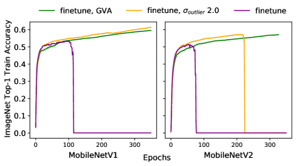
Figure 3: The gradient variance aware (GVA) method provides an additional benefit of de-emphasizing outliers during training, where the average second order moments ratios between the outliers and the inliers become smaller and are less than 1. MobileNetV1 and MobileNetV2 (4W4A) were able to be trained from scratch without the outlier method.

Figure 4 shows reduction in the average quantization error variance (left figure) and the average quantized weight $\it{fluctuation}$ variance (right figure) by using the GVA method for MobileNetV1 (see the Appendix C for MobileNetV2 results.).

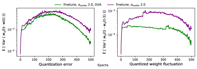
Figure 4: Gradient variance aware optimization (GVA) reduces the variance in average quantization error (left figure) and the variance in average quantized weight $\it{fluctuation}$ (right figure) on MobileNetV1. The metrics were measured from the weights and averaged across all the layers.

3.2 Improving $\sf{GRAD}$

3.2.1 Convergence Instability of $\sf{GRAD}$

Stably training the gradient-based hardware-friendly quantizer requires considerations for scaling factor convergence [15]. Figure 5 shows running-averaged PO2 scaling factors of $\sf{GRAD}$ and $\sf{MSQE}$ $(\sf{finetune},\sigma_{outlier}2.0,GVA)$ from a layer of MobileNetV1. We can see that there was more fluctuation in the PO2 scaling factor ($\Delta_{PO2}$) for $\sf{GRAD}$ than $\sf{MSQE}$ $(\sf{finetune},\sigma_{outlier}2.0,GVA)$. It is more evidently shown in Figure 6, which captured (per training step) the PO2 scaling factor exponent ($\log_{2}\Delta_{PO2})$ of both quantizers.

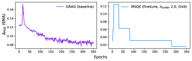
Figure 5: The running averages of PO2 scaling factors of $\sf{GRAD}$ and $\sf{MSQE}$ $(\sf{finetune},$ $\sigma_{outlier}$ $2.0,$ $\sf{GVA})$ of a MobileNetV1 layer.

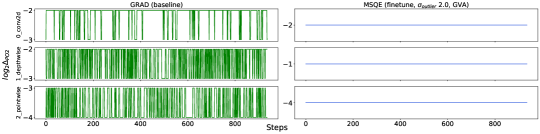
Figure 6: The (per-training step) PO2 scaling factor exponents of $\sf{GRAD}$ and $\sf{MSQE}$ $(\sf{finetune},$ $\sigma_{outlier}2.0,$ $\sf{GVA})$ in the first 3 layers of MobileNetV1 for 3 epochs starting from the 150th epoch.

Scaling factor oscillation around the ceil (round) transition boundary

As shown in Figure 6, the PO2 scaling factor fluctuates between the two adjacent PO2 scaling factors when the scaling factor exponent ($\Delta_{\log_{2}}$) oscillates around the transition boundary of the ceil (round) function (see (3)). To improve this type of instability, we adopt the idea from $\sf{MSQE}$ that uses an MSQE-optimal PO2 scaling factor instead of statically performing ceil (round) function. For example, if we choose to round to a lower MSQE PO2 scaling factor between the adjacent PO2 scaling factors, it can reduce the fluctuation when the (unconstrained) scaling factor ($2^{\Delta_{\log_{2}}}$) is near a locally MSQE minimum PO2 scaling factor as shown in Figure 7 (we call the method $\sf{RTLM}$ (Round-to-Lower-MSQE) (see Appendix D.1 for detailed algorithm).

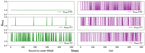
Figure 7: The effectiveness of $\sf{RTLM}$ (Round-to-Lower-MSQE) in improving the convergence instability to various random Gaussian noise perturbations to the input ($w$) for a toy example. It is a single quantizer configured to minimize the L2 error loss of $(w-Q(w,\Delta_{PO2}))^{2}$ using Adam [17] optimizer, where the (unconstrained) scaling factor ($2^{\Delta_{\log_{2}}}$) is initialized to near a locally MSQE minimum PO2 scaling factor ($1.0$) and the transition boundary of the ceil function.

Scaling factor oscillation at convergence

There is another type of convergence instability for $\sf{GRAD}$. Since the scaling factor is constrained to be a power-of-2 integer value, it cannot remain converged when an optimal scaling factor for a given input is not an exact power-of-2 integer value [15] as shown in Figure 8. This can be a problematic especially near the end of training, where the weights are nearly fixed. It can be solved by freezing the scaling factor and using a running-averaged PO2 scaling factor instead at convergence (see Appendix D.2 for the method in details.).

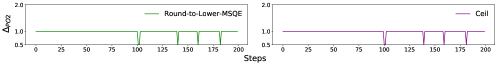
Figure 8: The PO2 scaling factors for both methods periodically fluctuate between 0.5 and 1 when the optimal (unconstrained) scaling factor for the loss function is about 0.9 for a given fixed input (it used the same settings as in Figure 7).

4 Experimental Results

We evaluate the MSQE-based and the gradient-based quantizers on MobileNetV1 [12] and MobileNetV2 [26] which are one of the most popular backbone architectures for custom ML hardwares .

4.1 Experimental Settings

We compare our $\sf{MSQE}$ improvements with the baseline implementation from QKeras [7]. [15] is our baseline for $\sf{GRAD}$. MobileNetV1 and MobileNetV2 are quantized into 4 bits weight and 4 bits activation (including the first and the last layers) and 8 bits bias. (The bias is quantized into more bits than weights because it is a small fraction of the parameters in the network, and keeping higher precision for bias is important since each bias affects many output activations [14, 22].) In all experiments we use $\sf{GRAD}$ to quantize the activation outputs. We ran each experiment 3 times and show the median run on the plots (wrt validation accuracy) as well as standard deviation ($\pm$) of results.

The models were trained from scratch on the ImageNet [25] dataset to see their quantization characteristics during entire training process. It was optimized using Adam [17] optimizer, the batch of 4096, the initial learning rate of 0.01, and cosine learning rate decay [21] with alpha of 0.001 and no warm restart, which were trained on TPU for 500 epochs. The training was regularized by random crop and random brightness saturation.

4.2 Evaluation of the Gradient Variance Awareness (GVA) Heuristic for $\sf{MSQE}$

We performed an experiment to see how much the presence of the GVA method can affect the overall performance. As we can see from Figure 9, adding the GVA method to the outlier mask only methods improved overall training stability and the validation accuracies (see the Appendix E.1 for training curves in detail and an additional ablation study.).

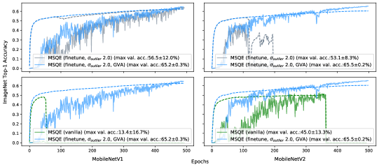
Figure 9: (Top figures) Adding gradient variance awareness (GVA) results in better training accuracy (solid line), better validation accuracy (dotted line), and greater robustness (lower standard deviation at end of training). (Bottom figures) We can see that the optimization instability issues in $\sf{MSQE}$ were fixed by the techniques that we presented. We show the median run (out of 3).

Figure 10 shows the overall performance improvements over the baseline MSQE quantization (even without the fine-tuning line search). Applying all the proposed techniques for the MSQE quantization made the optimization problem stable without any other adjustments or regularizers, allowing it to reach over 65% accuracy in both models.

4.3 Evaluation of RTLM for $\sf{GRAD}$

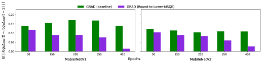
Figure 16: It shows average scaling factor exponent fluctuations (per training step) for training MobileNetV1 and MobileNetV2 for 3 epochs from the corresponding epochs on the x-axis. We can see that RTLM had less average scaling factor exponent fluctuations compared to the ceil function.

Figure 10 shows the effectiveness of RTLM method in improving training stability (based on the validation accuracy fluctuations). This can be explained by Figure 16 (in Appendix E.2) that measured the amount of scaling factor exponent changes (per training step) averaged across all the layers for 3 epochs from the corresponding epochs on the x-axis. We can see that RTLM had less average scaling factor fluctuations compared to the ceil function.

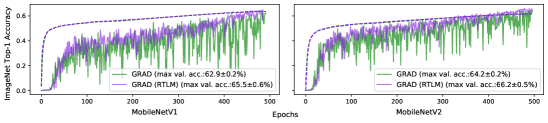
Figure 10: It shows the effectiveness of RTLM method in improving training stability (based on the validation accuracy (solid line) fluctuations). Validation accuracy improved by $2.6\%$ and $2.0\%$ for MobileNetV1 and MobileNetV2, respectively.

4.4 Evaluation of Freezing the Scaling Factor at Convergence for $\sf{GRAD}$

Freezing the scaling factor and using the running averaged scaling factor at convergence (at the 470th epoch) and fine-tuning the weights (for 30 epochs) further improved the validation accuracies for MobileNetV1 (MobileNetV2) for $\sf{GRAD}$ and $\sf{MSQE}$ to $66.9\pm 0.17\%$ ($67.5\pm 0.01\%$) and $65.6\pm 0.18\%$ ($66.5\pm 0.24\%$) respectively.

5 Conclusions

In this paper, we evaluated the two main classes of hardware-friendly quantization methods in the context of weight quantization: the traditional MSQE (Mean Squared Quantization Error)-based methods [7] and the more recent gradient-based methods [15]. We studied the two methods using multiple empirical metrics to identify the sources (underlying causes) of performance difference between the two classes, and found that the outliers in the input and the scaling factor convergence instabilities are main problems for the MSQE-based and the gradient-based methods respectively. Using our insights, we proposed various techniques to improve the performance of both quantizers, which provided stability of the MSQE-based training and increased the validation accuracy of the gradient-based methods by 4.0% and 3.3% for MobileNetV1 [12] and MobileNetV2 [26] on ImageNet [25] respectively. We believe that our insights could also be useful for activation quantization but leave that for future work.

Appendices

Appendix A Details on Sub-optimality in the Optimization of $\sf{MSQE}$

As shown in the example below (signed 4 bit quantization), it converges to a sub-optimal PO2 scaling factor of 1.0 for the initial scaling factor ($\Delta_{init}$) of 1.0, where 2.0 is an MSQE-optimal PO2 scaling factor (see figure 11). This sub-optimality can be improved by using a line search algorithm as in Algorithm 2, where it simply searches for an MSQE-optimal PO2 scaling factor from the vicinity of the solution from Algorithm 1.

$$\text{Inputs}: w =\begin{pmatrix}-0.17&2.58&-8.75\\ -3.56&1.56&-0.15\\ 2.15&-0.66&0.49\end{pmatrix},\;\Delta_{init}=1.0,N_{iters}=2$$

$$\text{$1_{st}$ iteration}: q=\frac{Q(w,\Delta_{init})}{\Delta_{init}} =\begin{pmatrix}0.0&3.0&-7.0\\ -4.0&2.0&0.0\\ 2.0&-1.0&0.0\end{pmatrix}\Rightarrow\Delta_{1_{st}}=1.0=PO2(\cfrac{91.31}{83.0})$$ (8)

$$\text{$2_{nd}$ iteration}: q=\frac{Q(w,\Delta_{1_{st}})}{\Delta_{1_{st}}} =\begin{pmatrix}0.0&3.0&-7.0\\ -4.0&2.0&0.0\\ 2.0&-1.0&0.0\end{pmatrix}\Rightarrow\Delta_{2_{nd}}=1.0=PO2(\cfrac{91.31}{83.0})$$

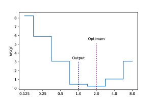
Figure 11: It shows the MSQE for various PO2 scaling factors (x-axis) from the vicinity of the output (1.0) of Algorithm 1 for an example in (8). We can see that 1.0 is not an MSQE-optimal PO2 scaling factor.

Algorithm 2 Line Search

$w,{\Delta}_{PO2_{init}},{N}_{range}$

${\Delta_{PO2}^{*}}$

procedure :

     $w_{q}\leftarrow Q(w,{\Delta}_{PO2_{init}})$

     $msqe^{*}\leftarrow||w_{q}-w||^{2}$

     $\Delta_{PO2}^{*}\leftarrow{\Delta}_{PO2_{init}}$

     for $offset$ = $-N_{range}$ to ${N}_{range}$ do

         $\Delta_{PO2}\leftarrow{\Delta}_{PO2_{init}}\cdot 2^{offset}$

         $w_{q}\leftarrow Q(w,\Delta_{PO2})$

         $msqe\leftarrow||w_{q}-w||^{2}$

         if $msqe<msqe^{*}$ then:

              $msqe^{*}\leftarrow msqe$

              $\Delta_{PO2}^{*}\leftarrow\Delta$

         end if

     end for

end procedure

Appendix B Details on a Problem with Outliers in $\sf{MSQE}$

The equation (9) (copied here for convenience) shows that a percentile based threshold ($\sigma_{outlier}$) is used to generate an outlier mask for the MSQE optimization to filter out outliers. Each element in the outlier mask gets either 1 or 0 depending on whether its corresponding input value is less than the threshold. Algorithm 3 and 4 show how the outlier mask is applied during the MSQE optimizations. They get the outlier mask as a weight factor ($f_{msqe}$), which is possibly combined (multiplied) with other weight factors, and perform a weighed least squares fit and a weighted line search to ignore the outliers as shown in Algorithm 3 and 4, respectively.

$$M_{outlier}=\begin{cases}0&\text{if }|w|\geq\sigma_{outlier}\cdot\sigma(w)\\ 1&\text{if }|w|<\sigma_{outlier}\cdot\sigma(w)\end{cases}$$ (9)

Algorithm 3 Weighted MSQE-based Quantizer Optimization

$w,{\Delta}_{init},{N}_{iters},f_{msqe}$

${\Delta_{PO2}}$

procedure :

     $q\leftarrow\frac{Q(w,\Delta_{init})}{\Delta_{init}}$

     $q\leftarrow q\odot\sqrt{f_{msqe}}$ $\triangleright$ Apply the element-wise MSQE weight factor.

     $w\leftarrow w\odot\sqrt{f_{msqe}}$ $\triangleright$ Apply the element-wise MSQE weight factor.

     $N\leftarrow{N}_{iters}$

     while $N\neq 0$ do

         $\Delta\leftarrow\cfrac{q^{T}w}{q^{T}q}$ $\triangleright$ Find an unconstrained optimal $\Delta$ minimizing the MSQE.

         $\Delta_{PO2}\leftarrow PO2(\Delta)$ $\triangleright$ Constrain $\Delta$ to be PO2.

         $q\leftarrow\frac{Q(w,\Delta_{PO2})}{\Delta_{PO2}}$ $\triangleright$ Quantize w with the newly found $\Delta_{PO2}$.

         $q\leftarrow q\odot\sqrt{f_{msqe}}$ $\triangleright$ Apply the element-wise MSQE weight factor.

         $N\leftarrow N-1$

     end while

end procedure

Algorithm 4 Weighted Line Search

$w,{\Delta}_{PO2_{init}},{N}_{range},f_{msqe}$

${\Delta_{PO2}^{*}}$

procedure :

     $w_{q}\leftarrow Q(w,{\Delta}_{PO2_{init}})$

     $msqe^{*}\leftarrow||f_{msqe}\odot(w_{q}-w)||^{2}$ $\triangleright$ Apply the element-wise MSQE weight factor.

     $\Delta_{PO2}^{*}\leftarrow{\Delta}_{PO2_{init}}$

     for $offset$ = $-N_{range}$ to ${N}_{range}$ do

         $\Delta_{PO2}\leftarrow{\Delta}_{PO2_{init}}\cdot 2^{offset}$

         $w_{q}\leftarrow Q(w,\Delta_{PO2})$

         $msqe\leftarrow||f_{msqe}\odot(w_{q}-w)||^{2}$ $\triangleright$ Apply the element-wise MSQE weight factor.

         if $msqe<msqe^{*}$ then:

              $msqe^{*}\leftarrow msqe$

              $\Delta_{PO2}^{*}\leftarrow\Delta$

         end if

     end for

end procedure

Appendix C Details on Gradient Variance Awareness (GVA) Heuristic for Loss-Aware Optimization of $\sf{MSQE}$

The figure 13 shows reduction in the average quantization error variance (left figure) and the average quantized weight $\it{fluctuation}$ variance (right figure) by using the gradient variance aware (GVA) MSQE optimization for MobileNetV2 (the metrics were measured from the weights and averaged across all the layers).

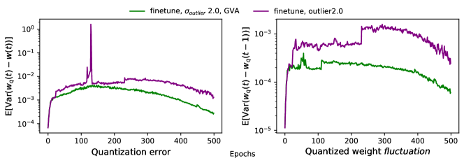
Figure 13: It shows reduction in the average quantization error variance (left figure) and the average quantized weight $\it{fluctuation}$ variance (right figure) by using the gradient variance aware (GVA) MSQE optimization for MobileNetV2.

Appendix D Details on Convergence Instability of $\sf{GRAD}$

D.1 Scaling factor oscillation around the ceil (round) transition boundary

Algorithm 5 describes the method in detail. It gets the weight ($w$), the unconstrained step-size ($\Delta_{\log_{2}}$), the running averaged second order moments of the weight ($v_{w}$), and an outlier mask ($M_{{outlier}^{\Delta_{\log_{2}}}}$) shown in (10). Then it calculates weighted MSQEs of ${\Delta}_{PO2_{\operatorname{ceil}}}$ and ${\Delta}_{PO2_{\operatorname{floor}}}$ to find a PO2 step-size with lower MSQE.

$$M_{{outlier}^{\Delta_{\log_{2}}}}=\begin{cases}0&\text{if }|w|\geq q_{max}\cdot 2^{\Delta_{\log_{2}}}\\ 1&\text{if }|w|<q_{max}\cdot 2^{\Delta_{\log_{2}}}\end{cases}$$ (10)

Algorithm 5 RTLM (Round-to-Lower-MSQE)

$w,{\Delta_{\log_{2}}},v_{w},M_{{outlier}^{\Delta_{\log_{2}}}}$

${\Delta_{PO2}^{*}}$

procedure :

     ${\Delta}_{PO2_{\operatorname{ceil}}}\leftarrow 2^{\operatorname{ceil}(\Delta_{\log_{2}})}$

     ${\Delta}_{PO2_{\operatorname{floor}}}\leftarrow 2^{\operatorname{floor}(\Delta_{\log_{2}})}$

     $msqe_{\operatorname{ceil}}\leftarrow||M_{{outlier}^{\Delta_{\log_{2}}}}\odot v_{w}\odot(Q(w,{\Delta}_{PO2_{\operatorname{ceil}}})-w)||^{2}$

     $msqe_{\operatorname{floor}}\leftarrow||M_{{outlier}^{\Delta_{\log_{2}}}}\odot v_{w}\odot(Q(w,{\Delta}_{PO2_{\operatorname{floor}}})-w)||^{2}$

     if $msqe_{\operatorname{ceil}}<msqe_{\operatorname{floor}}$ then:

         $\Delta_{PO2}^{*}\leftarrow{\Delta}_{PO2_{\operatorname{ceil}}}$

     else:

         $\Delta_{PO2}^{*}\leftarrow{\Delta}_{PO2_{\operatorname{floor}}}$

     end if

end procedure

D.2 Scaling factor oscillation at convergence

Algorithm 6 describes the freezing method to improve the scaling factor instability at convergence. It estimates a running average of the PO2 scaling factor exponent ($EMA_{\log_{2}\Delta_{\operatorname{PO2}}}$) and returns the PO2 scaling factor based on $EMA_{\log_{2}\Delta_{\operatorname{PO2}}}$ only when the indicator ($\mathbbm{1}_{freeze}$) value is set true.

Algorithm 6 Running-Averaged PO2 Step-Size

$\Delta_{\operatorname{PO2}},\mathbbm{1}_{freeze}$

$\Delta_{\operatorname{PO2}}$

procedure :

     if $\mathbbm{1}_{freeze}$ then:

         $\beta\leftarrow 1.0$

     end if

     $EMA_{\log_{2}\Delta_{\operatorname{PO2}}}\leftarrow\beta\cdot EMA_{\log_{2}\Delta_{\operatorname{PO2}}}+(1.0-\beta)\cdot log_{2}(\Delta_{\operatorname{PO2}})$

     if $\mathbbm{1}_{freeze}$ then:

         $\Delta_{\operatorname{PO2}}\leftarrow 2^{\operatorname{round}(EMA_{\log_{2}\Delta_{\operatorname{PO2}}})}$

     else:

         $\Delta_{\operatorname{PO2}}\leftarrow\Delta_{\operatorname{PO2}}$

     end if

end procedure

Appendix E Extended Results

E.1 Evaluation of the Gradient Variance Awareness (GVA) Heuristic for $\sf{MSQE}$

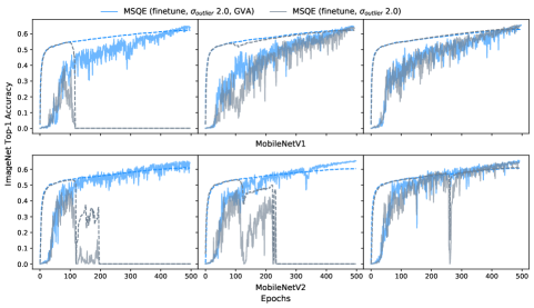
Figure 14: It shows all the three training curves for each of MobileNetV1 (top three figures) and MobileNetV2 (bottom three figures) with and without the GVA method. We can see that the outlier mask method alone ($\sf{MSQE}(finetune,\sigma_{outlier}2.0)$) resulted in training instability for MobileNetV1 and MobileNetV2.

We performed an ablation study to see how much the outlier method has an impact on the overall performance in the experiment in Section 4.2. As we can see from the figure 15, adding the outlier method to $\sf{MSQE}(finetune,GVA)$ (the GVA only method) improved training stability in the early epochs and the validation accuracy.

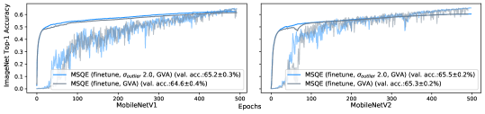
Figure 15: Adding the outlier method to $\sf{MSQE}(finetune,GVA)$ improved training stability in the early epochs and the validation accuracy.

E.2 Evaluation of RTLM of $\sf{GRAD}$

References

- Anwar et al. [2015] Sajid Anwar, Kyuyeon Hwang, and Wonyong Sung. Fixed point optimization of deep convolutional neural networks for object recognition. In 2015 IEEE International Conference on Acoustics, Speech and Signal Processing (ICASSP), pages 1131–1135, 2015. doi: 10.1109/ICASSP.2015.7178146.
- au2 et al. [2021] Claudionor N. Coelho Jr. au2, Aki Kuusela, Shan Li, Hao Zhuang, Thea Aarrestad, Vladimir Loncar, Jennifer Ngadiuba, Maurizio Pierini, Adrian Alan Pol, and Sioni Summers. Automatic heterogeneous quantization of deep neural networks for low-latency inference on the edge for particle detectors, 2021.
- Bengio et al. [2013] Yoshua Bengio, Nicholas Léonard, and Aaron Courville. Estimating or propagating gradients through stochastic neurons for conditional computation, 2013.
- Bhalgat et al. [2020] Yash Bhalgat, Jinwon Lee, Markus Nagel, Tijmen Blankevoort, and Nojun Kwak. Lsq+: Improving low-bit quantization through learnable offsets and better initialization. 2020 IEEE/CVF Conference on Computer Vision and Pattern Recognition Workshops (CVPRW), pages 2978–2985, 2020.
- Choi et al. [2018] Jungwook Choi, Zhuo Wang, Swagath Venkataramani, Pierce I-Jen Chuang, Vijayalakshmi Srinivasan, and Kailash Gopalakrishnan. Pact: Parameterized clipping activation for quantized neural networks, 2018.
- Choi et al. [2017] Yoojin Choi, Mostafa El-Khamy, and Jungwon Lee. Towards the limit of network quantization, 2017.
- Coelho et al. [2020] Claudionor N. Coelho, Aki Kuusela, Shan Li, Hao Zhuang, Thea Aarrestad, Vladimir Loncar, Jennifer Ngadiuba, Maurizio Pierini, Adrian Alan Pol, and Sioni Summers. Ultra low-latency, low-area inference accelerators using heterogeneous deep quantization with qkeras and hls4ml. 2020. doi: 10.48550/ARXIV.2006.10159. URL https://github.com/google/qkeras.
- Esser et al. [2020] Steven K. Esser, Jeffrey L. McKinstry, Deepika Bablani, Rathinakumar Appuswamy, and Dharmendra S. Modha. Learned step size quantization, 2020.
- Habi et al. [2020] Hai Victor Habi, Roy H. Jennings, and Arnon Netzer. Hmq: Hardware friendly mixed precision quantization block for cnns, 2020.
- Hou and Kwok [2018] Lu Hou and James T. Kwok. Loss-aware weight quantization of deep networks, 2018.
- Hou et al. [2018] Lu Hou, Quanming Yao, and James T. Kwok. Loss-aware binarization of deep networks, 2018.
- Howard et al. [2017] Andrew G. Howard, Menglong Zhu, Bo Chen, Dmitry Kalenichenko, Weijun Wang, Tobias Weyand, Marco Andreetto, and Hartwig Adam. Mobilenets: Efficient convolutional neural networks for mobile vision applications, 2017.
- Ioffe and Szegedy [2015] Sergey Ioffe and Christian Szegedy. Batch normalization: Accelerating deep network training by reducing internal covariate shift, 2015.
- Jacob et al. [2017] Benoit Jacob, Skirmantas Kligys, Bo Chen, Menglong Zhu, Matthew Tang, Andrew Howard, Hartwig Adam, and Dmitry Kalenichenko. Quantization and training of neural networks for efficient integer-arithmetic-only inference, 2017.
- Jain et al. [2020] Sambhav R. Jain, Albert Gural, Michael Wu, and Chris H. Dick. Trained quantization thresholds for accurate and efficient fixed-point inference of deep neural networks, 2020.
- Jung et al. [2018] Sangil Jung, Changyong Son, Seohyung Lee, Jinwoo Son, Youngjun Kwak, Jae-Joon Han, Sung Ju Hwang, and Changkyu Choi. Learning to quantize deep networks by optimizing quantization intervals with task loss, 2018.
- Kingma and Ba [2017] Diederik P. Kingma and Jimmy Ba. Adam: A method for stochastic optimization, 2017.
- Krishnamoorthi [2018] Raghuraman Krishnamoorthi. Quantizing deep convolutional networks for efficient inference: A whitepaper, 2018.
- Kunstner et al. [2019] Frederik Kunstner, Philipp Hennig, and Lukas Balles. Limitations of the empirical fisher approximation for natural gradient descent. In NeurIPS, 2019.
- Li et al. [2020] Yuhang Li, Xin Dong, and Wei Wang. Additive powers-of-two quantization: An efficient non-uniform discretization for neural networks, 2020.
- Loshchilov and Hutter [2017] Ilya Loshchilov and Frank Hutter. Sgdr: Stochastic gradient descent with warm restarts, 2017.
- Lyon and Yaeger [1996] R.F. Lyon and Larry Yaeger. On-line hand-printing recognition with neural networks. pages 201–212, 03 1996. ISBN 0-8186-7373-7. doi: 10.1109/MNNFS.1996.493792.
- Park and Yoo [2020] Eunhyeok Park and Sungjoo Yoo. Profit: A novel training method for sub-4-bit mobilenet models, 2020.
- Rastegari et al. [2016] Mohammad Rastegari, Vicente Ordonez, Joseph Redmon, and Ali Farhadi. Xnor-net: Imagenet classification using binary convolutional neural networks, 2016.
- Russakovsky et al. [2015] Olga Russakovsky, Jia Deng, Hao Su, Jonathan Krause, Sanjeev Satheesh, Sean Ma, Zhiheng Huang, Andrej Karpathy, Aditya Khosla, Michael Bernstein, Alexander C. Berg, and Li Fei-Fei. Imagenet large scale visual recognition challenge, 2015.
- Sandler et al. [2019] Mark Sandler, Andrew Howard, Menglong Zhu, Andrey Zhmoginov, and Liang-Chieh Chen. Mobilenetv2: Inverted residuals and linear bottlenecks, 2019.
- Wang et al. [2019] Erwei Wang, James J. Davis, Ruizhe Zhao, Ho-Cheung Ng, Xinyu Niu, Wayne Luk, Peter Y. K. Cheung, and George A. Constantinides. Deep neural network approximation for custom hardware. ACM Computing Surveys, 52(2):1–39, May 2019. ISSN 1557-7341.
- Yang et al. [2019] Jiwei Yang, Xu Shen, Jun Xing, Xinmei Tian, Houqiang Li, Bing Deng, Jianqiang Huang, and Xiansheng Hua. Quantization networks, 2019.
- Zhang et al. [2018] Dongqing Zhang, Jiaolong Yang, Dongqiangzi Ye, and Gang Hua. Lq-nets: Learned quantization for highly accurate and compact deep neural networks, 2018.
- Zhen et al. [2019] Dong Zhen, Zhewei Yao, Amir Gholami, Michael Mahoney, and Kurt Keutzer. Hawq: Hessian aware quantization of neural networks with mixed-precision. pages 293–302, 10 2019.